Petrovič Inequality and Its Associated Midpoint- and Trapezoid-Type Estimates with Fractional Extensions for Superquadraticity via Multiplicative Calculus

Abstract

In this paper, we establish a novel Petrovič-type inequality together with new integral identities for multiplicatively superquadratic functions within the framework of multiplicative calculus. By employing these foundational results, we derive midpoint- and trapezoid-type inequalities for this class of functions, including their fractional analogues formulated via multiplicative Riemann–Liouville fractional operators. The theoretical findings are supported through detailed numerical computations and graphical illustrations, supporting the theoretical results. Furthermore, the applicability of the developed inequalities is demonstrated through representative examples involving special means and the modified Bessel function of type I, thereby highlighting the analytical significance and practical relevance of the obtained results.

1. Motivation and Background

The fundamental role of inequalities associated with convex functions has been recognized since the early stages of mathematical analysis. Over time, these inequalities have emerged as essential tools that significantly influence the advancement of numerous contemporary areas of mathematics. Consequently, they have attracted sustained and substantial attention in the mathematical literature due to their theoretical depth and wide-ranging applications. Some famous results for such estimations consist of Hermite–Hadamard, midpoint, trapezoid, Simpson or Jensen inequalities, etc.

Let $\mathrm{{\rm Y}}:\mathrm{I}\subset \mathrm{R}\to \mathrm{R}$ be a convex mapping defined on the interval $\mathrm{I}$ of real numbers and $\vartheta ,\upsilon \in \mathrm{I}$, with $\vartheta <\upsilon$. The double inequality presented below is commonly cited in the literature as the Hermite–Hadamard inequalities [1]:

$$\mathrm{{\rm Y}}\left({\displaystyle \frac{\vartheta +\upsilon }{2}}\right)\le {\displaystyle \frac{1}{\upsilon -\vartheta }}{\int }_{\vartheta }^{\upsilon }\mathrm{{\rm Y}}\left(\varkappa \right)d\varkappa \le {\displaystyle \frac{\mathrm{{\rm Y}}\left(\vartheta \right)+\mathrm{{\rm Y}}\left(\upsilon \right)}{2}}.$$

(1)

In the theory of convex functions, the Hermite–Hadamard inequalities constitute a cornerstone result for estimating the integral mean. It provides sharp two-sided bounds for the integral mean of a convex function and simultaneously guarantees the integrability of such functions on closed intervals. This property is of substantial theoretical interest, as several classical mean inequalities can be derived directly from Hadamard’s inequality through appropriate choices of particular convex functions $\mathrm{{\rm Y}}$. Inequalities of this type constitute fundamental tools in mathematical analysis and have far-reaching implications across diverse domains of pure and applied mathematics. In the literature, the absolute value of the difference in the second part of the (1) inequalities is recognized as the trapezoidal inequality, first established by Dragomir and Agarwal in 1998 [2]. Subsequently, in 2004, Kirmaci introduced the absolute value of the difference in the first part of the (1) inequalities, which is commonly referred to as the midpoint inequality [3].

Motivated by the desire to obtain sharper estimates and to extend these results beyond classical convexity, several generalized convexity notions have been introduced. Among them, superquadratic functions stand out for their richer geometric structure and their effectiveness in refining Jensen- and Hermite–Hadamard-type inequalities. We therefore turn to the theory of superquadraticity, beginning with a brief review of the geometric interpretation of convex functions. Let $(\vartheta ,\mathrm{{\rm Y}}(\vartheta \left)\right)$ and $(\upsilon ,\mathrm{{\rm Y}}(\upsilon \left)\right)$ be two points on the graph of a function $\mathrm{{\rm Y}}$ on or below the chord connecting the endpoints for every $\vartheta ,\upsilon \in \mathrm{I}$, with $\vartheta \le \upsilon$. Symbolically, it is expressed as

$$\mathrm{{\rm Y}}\left(\varkappa \right)\le {\displaystyle \frac{\mathrm{{\rm Y}}\left(\upsilon \right)-\mathrm{{\rm Y}}\left(\vartheta \right)}{\upsilon -\vartheta }}(\varkappa -\vartheta )+\mathrm{{\rm Y}}\left(\vartheta \right),$$

(2)

for every $\vartheta \le \varkappa \le \upsilon$. Alternatively, for a function $\mathrm{{\rm Y}}:\mathrm{I}\to \mathrm{R}$, we say that $\mathrm{{\rm Y}}$ possesses a supporting line at a point $\vartheta \in \mathrm{I}$, if there exists a real number ${\mathfrak{C}}_{\vartheta }$ such that

$$\mathrm{{\rm Y}}\left(\varkappa \right)\ge \mathrm{{\rm Y}}\left(\vartheta \right)+{\mathfrak{C}}_{\vartheta }(\varkappa -\vartheta ),$$

(3)

for every $\varkappa \in \mathrm{I}$. The collection of all such ${\mathfrak{C}}_{\vartheta }$ is referred to as the subdifferential of $\mathrm{{\rm Y}}$ at the point $\vartheta$, and it is designated by $\partial \mathrm{{\rm Y}}$. In essence, the subdifferential describes the slopes of all lines that support the graph of $\mathrm{{\rm Y}}$ from below. Therefore, if $\mathrm{{\rm Y}}$ is convex, then the subdifferential $\partial \mathrm{{\rm Y}}$ is non-empty at all interior points of its domain.

From this perspective, Abramovich et al. [4] extended the above concept to what they termed superquadratic functions.

Definition 1.

A function $\mathrm{{\rm Y}}:[0,\infty )⟶R$ is called superquadratic provided that for every $\vartheta \ge 0$, there exists a constant ${\mathfrak{C}}_{\vartheta }\in \mathrm{R}$ such that the inequality

$$\mathrm{{\rm Y}}\left(\varkappa \right)\ge \mathrm{{\rm Y}}\left(\vartheta \right)+{\mathfrak{C}}_{\vartheta }(\varkappa -\vartheta )+\mathrm{{\rm Y}}\left(\right|\varkappa -\vartheta \left|\right),$$

(4)

holds $\forall \varkappa \ge 0$. Thus, for a superquadratic function, we require that Y lies above its tangent line plus a translation of Y itself.

Remark 1.

If the function Y is superquadratic, then its negation $-\mathrm{{\rm Y}}$ is subquadratic. Consequently, the inequality in (4) is reversed.

Example 1.

The function $\mathrm{{\rm Y}}\left(\varkappa \right)={\varkappa }^{\mathfrak{n}}$ defined for $\varkappa \ge 0$ and $\mathfrak{n}\ge 2$ is superquadratic, whereas it is subquadratic when $0\le \mathfrak{n}<2$. In this context, ${\mathfrak{C}}_{\varkappa }=\mathfrak{n}{\varkappa }^{\mathfrak{n}-1}$. Moreover, equality holds in (4), when $\mathfrak{n}=2$.

The following lemma is based on the definition of superquadraticity, and any function which fulfills the conditions mentioned in this lemma is considered as superquadratic, such that the functions $\mathrm{{\rm Y}}\left(\varkappa \right)={\varkappa }^{2}ln\varkappa$ for $\varkappa >0$ and $sign(\mathfrak{n}-2){\varkappa }^{\mathfrak{n}}$ for $\mathfrak{n}\ge 1$ are superquadratic.

Lemma 1.

Suppose that $\mathrm{{\rm Y}}:[0,\infty )\to \mathrm{R}$ is continuously differentiable and satisfies $\mathrm{{\rm Y}}\left(0\right)\le 0$. If ${\mathrm{{\rm Y}}}^{\prime }$ is superadditive, or if the function ${\displaystyle \frac{{\mathrm{{\rm Y}}}^{\prime }\left(\varkappa \right)}{\varkappa }}$ is non-decreasing on $(0,\infty )$, then Y is superquadratic.

The concept of superquadratic functions, along with a fundamental description, was formulated by Abramovich and his colleagues in [4,5]. Condition (4) is seemingly more effective than the usual convexity criterion. The above-mentioned claim is valid for a superquadratic function provided it is non-negative, but it is worth noting that if $\mathrm{{\rm Y}}$ assumes negative values, it may be considered a weaker function in terms of its superquadraticity. Therefore, if $\mathrm{{\rm Y}}$ is superquadratic and non-negative, then $\mathrm{{\rm Y}}$ is convex and increasing, as demonstrated in [4]. More precisely, a randomly selected superquadratic function satisfies the three subsequent requirements mentioned in Lemma 2:

Lemma 2

([4]). Let Y be a superquadratic function, then

1. 

$\mathrm{{\rm Y}}\left(0\right)\le 0$.

2. 

If Y is differentiable at $\varkappa >0$ and $\mathrm{{\rm Y}}\left(0\right)={\mathrm{{\rm Y}}}^{\prime }\left(0\right)=0$, then ${\mathrm{{\rm Y}}}^{\prime }\left(\varkappa \right)={\mathfrak{C}}_{\varkappa }$.

3. 

Y is termed as convex if $\mathrm{{\rm Y}}\ge 0$ and $\mathrm{{\rm Y}}\left(0\right)={\mathrm{{\rm Y}}}^{\prime }\left(0\right)=0$.

The following result provides a sufficient condition under which convexity (or concavity) implies superquadraticity (or subquadraticity).

Lemma 3

([4]). If Y is convex (or concave) and satisfies $\mathrm{{\rm Y}}\left(0\right)={\mathrm{{\rm Y}}}^{\prime }\left(0\right)=0$, then Y is superquadratic (or subquadratic). However, the converse of this statement does not necessarily hold.

Remark 2.

Subquadraticity does not necessarily imply concavity; in fact, some subquadratic functions are convex. For instance, the function $\mathrm{{\rm Y}}\left(\varkappa \right)={\varkappa }^{\mathfrak{n}}$, where $\varkappa \ge 0$ and $1\le \mathfrak{n}<2$, serves as a clear example of a function that is both subquadratic and convex.

One of the key definitions of a superquadratic function is the extension of Jensen’s inequality, given in its most basic form. Thus, the subsequent definition also applies to a superquadratic function [5].

Definition 2.

A function $\mathrm{{\rm Y}}:[0,\infty )⟶R$ is called superquadratic if the inequality

$$\begin{array}{l}\mathrm{{\rm Y}}((1-\gamma )\vartheta +\gamma \upsilon )\le (1-\gamma )\left[\mathrm{{\rm Y}}\left(\vartheta \right)-\mathrm{{\rm Y}}\left(\gamma \right|\vartheta -\upsilon \left|\right)\right]\\ +\gamma \left[\mathrm{{\rm Y}}\left(\upsilon \right)-\mathrm{{\rm Y}}\left(\right(1-\gamma \left)\right|\vartheta -\upsilon \left|\right)\right]\end{array}$$

(5)

holds, $\forall \vartheta ,\upsilon \ge 0$ and $0\le \gamma \le 1$.

Multiplicatively superquadratic function is another class of superquadraticity, introduced by Krnić et al. [6]. It is also termed as logarithmically superquadratic function. The definition of such a function that forms the foundation of this study is given below:

Definition 3.

A function $\mathrm{{\rm Y}}:[0,\infty )\to (0,\infty )$ is called multiplicatively superquadratic, if the inequality

$$\mathrm{{\rm Y}}((1-\gamma )\vartheta +\gamma \upsilon )\le {\displaystyle \frac{{\left[\mathrm{{\rm Y}}\left(\vartheta \right)\right]}^{1-\gamma }{\left[\mathrm{{\rm Y}}\left(\upsilon \right)\right]}^{\gamma }}{\left[\mathrm{{\rm Y}}\right(\gamma |\vartheta -{\upsilon \left|\right)]}^{1-\gamma }\left[\mathrm{{\rm Y}}\right((1-\gamma )|\vartheta -{\upsilon \left|\right)]}^{\gamma }}}$$

(6)

holds, ∀$\vartheta ,\upsilon \ge 0$ and $0\le \gamma \le 1$.

A function $\mathrm{{\rm Y}}$ is called multiplicatively superquadratic if the function $log\mathrm{{\rm Y}}$ exhibits superquadratic behavior. If a function $\mathrm{{\rm Y}}$ is multiplicatively subquadratic, then the inequality (6) flips. Only positive-valued functions can exhibit multiplicatively superquadraticity. If $\mathrm{{\rm Y}}$ is multiplicatively superquadratic, then $\mathrm{{\rm Y}}\left(0\right)\le 1$.

Let us state some important results related to the multiplicatively superquadratic function.

Theorem 1

([6]). Let $\mathrm{{\rm Y}}:[0,\infty )\to (0,\infty )$ be a multiplicatively superquadratic, then

$$\mathrm{{\rm Y}}((1-\gamma )\vartheta +\gamma \upsilon )\le {\left[\mathrm{{\rm Y}}\left(\vartheta \right)\right]}^{1-\gamma }{\left[\mathrm{{\rm Y}}\left(\upsilon \right)\right]}^{\gamma },$$

(7)

holds, ∀$\vartheta ,\upsilon \ge 0$ and $0\le \gamma \le 1$. It is worth noting that Y possesses the property of multiplicative convexity.

Remark 3.

As previously established, the power function $\mathrm{g}\left(\varkappa \right)={\varkappa }^{\mathfrak{n}}$ is superquadratic for $\mathfrak{n}\ge 2$ and subquadratic for $0<\mathfrak{n}\le 2$. Consequently, the function $\mathrm{{\rm Y}}\left(\varkappa \right)=exp\left\{{\varkappa }^{\mathfrak{n}}\right\}$ is multiplicatively superquadratic when $\mathfrak{n}\ge 2$, whereas it is multiplicatively subquadratic for $0<\mathfrak{n}\le 2$. Observe that Y takes values in the interval $[1,\infty )$. Therefore, in light of Theorem 1 and the preceding discussion, it follows that the function $\mathrm{{\rm Y}}\left(\varkappa \right)=exp\left\{{\varkappa }^{\mathfrak{n}}\right\}$ is convex for $\mathfrak{n}\ge 2$. On the other hand, it is well known that the power function $\mathrm{{\rm Y}}\left(\varkappa \right)={\varkappa }^{\mathfrak{n}}$ is convex on $[0,\infty )$ for all $\mathfrak{n}\ge 1$, since $\mathrm{g}\left(\varkappa \right)={\varkappa }^{\mathfrak{n}}$ is convex on this domain under the same condition.

Additional information on superquadratic functions, together with examples, properties, and applications to inequalities, can be found in the cited references [7,8,9,10].

While superquadratic functions provide a powerful refinement of convexity and lead to sharper integral inequalities in the classical additive setting, further improvements and alternative formulations can be achieved by employing non-additive analytical frameworks. In this context, multiplicative calculus emerges as a natural and effective tool for extending superquadratic inequalities beyond the traditional setting.

Innovative developments in mathematical analytical tools frequently transform associated fields. Multiplicative calculus, also known as non-Newtonian calculus, was introduced in 1967 by Grossman and Katz [11]. This innovative method substitutes multiplicative and divisional operators for the linear operations found in traditional calculus. Nonlinear processes like geometric growth and exponential dynamics are well modeled by this approach. Its multiplicative derivative is described as follows:

$${\mathrm{{\rm Y}}}^{\ast }\left(\varkappa \right)=\underset{\mathrm{h}\to 0}{lim}{\left({\displaystyle \frac{\mathrm{{\rm Y}}(\varkappa +\mathrm{h})}{\mathrm{{\rm Y}}\left(\varkappa \right)}}\right)}^{{\displaystyle \frac{1}{\mathrm{h}}}}.$$

(8)

Here, $\mathrm{{\rm Y}}\left(\varkappa \right)$ is a positive function; therefore, ${\displaystyle \frac{\mathrm{{\rm Y}}(\varkappa +\mathrm{h})}{\mathrm{{\rm Y}}\left(\varkappa \right)}}>0$ for sufficiently small $\mathrm{h}$. The function ${\mathrm{{\rm Y}}}^{\ast }\left(\varkappa \right)$ is differentiable if and only if the following limit exists. A nonzero value of the limit corresponds geometrically to the instantaneous logarithmic growth rate, indicating the degree of exponential variation. A brief review of the classical derivative is presented to set the stage for the multiplicative derivative (8).

$${\mathrm{{\rm Y}}}^{\prime }\left(\varkappa \right)=\underset{\mathrm{h}\to 0}{lim}{\displaystyle \frac{\mathrm{{\rm Y}}(\varkappa +\mathrm{h})-\mathrm{{\rm Y}}\left(\varkappa \right)}{\mathrm{h}}}.$$

(9)

The multiplicative derivative is built upon the replacement of subtraction with division and multiplication with exponentiation. This construction yields the following connection between ${\mathrm{{\rm Y}}}^{\ast }$ and the classical derivative ${\mathrm{{\rm Y}}}^{\prime }$, provided $\mathrm{{\rm Y}}$ has positive values and is differentiable at $\varkappa$.

$${\mathrm{{\rm Y}}}^{\ast }\left(\varkappa \right)=exp\left\{{\left(ln\mathrm{{\rm Y}}\right)}^{\prime }\left(\varkappa \right)\right\}.$$

(10)

Thus, ${\mathrm{{\rm Y}}}^{\ast }$ can be interpreted as the exponential of the ordinary derivative of $ln\mathrm{{\rm Y}}$. This intrinsic duality naturally leads to defining the multiplicative integral in an exponential form. Accordingly, Bashirov et al. [12] formulated the multiplicative integral as

$${\int }_{\vartheta }^{\upsilon }{\left(\mathrm{{\rm Y}}\left(\varkappa \right)\right)}^{d\varkappa }=exp\left\{{\int }_{\vartheta }^{\upsilon }ln\mathrm{{\rm Y}}\left(\varkappa \right)d\varkappa \right\},$$

(11)

Here, ${\int }_{\vartheta }^{\upsilon }{\left(\mathrm{{\rm Y}}\left(\varkappa \right)\right)}^{d\varkappa }$ indicates the product-based accumulation of infinitesimal contributions along $[\vartheta ,\upsilon ]$, assuming $\mathrm{{\rm Y}}\left(\varkappa \right)>0$. It should be noted that the superscript $d\varkappa$ plays the role of an exponential infinitesimal and is not a differential element; hence, it is essentially different from the term $d\varkappa$ used in the classical integral ${\int }_{\vartheta }^{\upsilon }\left(\mathrm{{\rm Y}}\left(\varkappa \right)\right)d\varkappa$. The former is associated with infinitesimal exponentiation in a multiplicative framework, whereas the latter reflects the infinitesimal increment characteristic of additive summation.

Through the exponential reconstruction of logarithmic integration outcomes, the multiplicative integral yields an accumulation process governed by the geometric mean. Replacing the linear superposition characteristic of Riemann integration with a multiplicative framework allows for accurate modeling of exponential trends commonly found in biological and financial systems. As an illustrative example, we examine the bacterial population growth model presented below.

$${\mathrm{{\rm Y}}}^{\prime }\left(\varkappa \right)=\mathrm{R}\left(\varkappa \right)\mathrm{{\rm Y}}\left(\varkappa \right).$$

(12)

In this model, the population size at time $\varkappa$ is given by $\mathrm{{\rm Y}}\left(\varkappa \right)$, while ${\mathrm{{\rm Y}}}^{\prime }\left(\varkappa \right)$ denotes its instantaneous rate of change and $\mathrm{R}\left(\varkappa \right)>0$ the associated multiplicative growth rate. Both time and growth rate are strictly positive. The equation characterizes an idealized process in which population growth is continuously proportional to its current size. In practical biological systems with finite resources, however, the growth rate $\mathrm{R}\left(\varkappa \right)>0$ declines as the population increases, requiring more realistic models such as the logistic equation.

An equivalent formulation of the differential Equation (12) is given by

$$exp\left\{{\left(ln\left(\mathrm{{\rm Y}}\right(\varkappa \left)\right)\right)}^{\prime }\right\}=exp\left\{\mathrm{R}\left(\varkappa \right)\right\}.$$

(13)

In view of the relation between ${\mathrm{{\rm Y}}}^{\ast }$ and ${\mathrm{{\rm Y}}}^{\prime }$ in (10), Equation (13) can be written as the multiplicative differential equation:

$${\mathrm{{\rm Y}}}^{\ast }\left(\varkappa \right)=exp\left\{\mathrm{R}\left(\varkappa \right)\right\}.$$

(14)

The solution of (14) using multiplicative integration is given by

$$\mathrm{{\rm Y}}\left(\varkappa \right)=\gamma {\int }_{{\varkappa }_o}^{\varkappa }{\left(exp\left\{\mathrm{R}\left(\varkappa \right)\right\}\right)}^{d\varkappa },\gamma =\mathrm{{\rm Y}}\left({\varkappa }_o\right),$$

(15)

where $\mathrm{{\rm Y}}\left({\varkappa }_o\right)$ specifies the initial condition for the population size.

Accordingly, this example elucidates the insightful intrinsic relationship between multiplicative calculus and the theory of differential equations. In contrast to Equation (12), the new differential control Equation (14) provides a more natural and succinct representation, explicitly reflecting the growth rate $\mathrm{R}\left(\varkappa \right)$ exhibiting exponential dynamics.

Such applications highlight the importance of multiplicative calculus in practical contexts and have consequently motivated extensive theoretical developments across diverse scientific disciplines. In the context of mathematical physics, multiplicative calculus provides a framework for refined geometric formulations, including the identification of fractional symmetries in Lorentz–Minkowski space [13] and the characterization of multiplicative manifold structures associated with Dirac systems [14]. In topology, it provides reformulations of difference sequence spaces [15] and supports the development of variational principles based on multiplicative calculus [16]. Collectively, these findings help bridge gaps in nonlinear geometric theory and enhance the existing analytical methodologies. Further applications are discussed in [12,17] and the references cited therein.

Fractional calculus is a branch of mathematics that generalizes traditional calculus by extending the concepts of derivatives and integrals to non-integer orders such as ${\displaystyle \frac{1}{2}}$, $\pi$, or any real number. In traditional calculus, derivatives and integrals are defined for functions of integer orders, such as first derivatives, second derivatives, and so on. However, fractional calculus allows for derivatives and integrals of non-integer orders [18]. Several fractional operators have been introduced, for example, generalized proportional fractional operators [19], Sarikaya fractional operators [20], Katugampola fractional operators [21], Atangana–Baleanu fractional operators [22], generalized Riemann–Liouville fractional operators [23], and conformable fractional operators [24]. These operators are necessary for the description of memory and hereditary properties in most engineering [25], computer science [26], and control science [27] literature.

A wide range of inequalities has been well studied in the classical setting; however, their generalization to multiplicative calculus is still limited, particularly for fractional operators. Abdeljawad and Grossman [28] contributed to closing this gap by introducing a redefinition of Riemann–Liouville fractional operators that unifies non-Newtonian or multiplicative calculus with fractional theory.

Definition 4.

The definitions of the multiplicative Riemann–Liouville fractional operators, denoted by ${}_{\vartheta }\mathrm{I}_{\ast }^{\beta }\mathrm{{\rm Y}}\left(\varkappa \right)$ and ${}_{\ast }\mathrm{I}_{\upsilon }^{\beta }\mathrm{{\rm Y}}\left(\varkappa \right)$, are presented separately for the case $\beta >0$.

$$\begin{array}{ll}{}_{\vartheta }\mathrm{I}_{\ast }^{\beta }\mathrm{{\rm Y}}\left(\varkappa \right)& =exp\{{\mathrm{I}}_{{\vartheta }^{+}}^{\beta }ln\mathrm{{\rm Y}}\left(\varkappa \right)\}\\ & =exp\left\{{\displaystyle \frac{1}{\mathsf{\Gamma }\left(\beta \right)}}{\int }_{\vartheta }^{\varkappa }{(\varkappa -\gamma )}^{\beta -1}ln\mathrm{{\rm Y}}\left(\gamma \right)\mathrm{d}\gamma \right\},\varkappa >\vartheta ,\end{array}$$

(16)

and

$$\begin{array}{ll}{}_{\ast }\mathrm{I}_{\upsilon }^{\beta }\mathrm{{\rm Y}}\left(\varkappa \right)& =exp\left\{{\mathrm{I}}_{{\upsilon }^{-}}^{\beta }ln\mathrm{{\rm Y}}\left(\varkappa \right)\right\}\\ & =exp\left\{{\displaystyle \frac{1}{\mathsf{\Gamma }\left(\beta \right)}}{\int }_{\varkappa }^{\upsilon }{(\gamma -\varkappa )}^{\beta -1}ln\mathrm{{\rm Y}}\left(\gamma \right)\mathrm{d}\gamma \right\},\varkappa <\upsilon ,\end{array}$$

(17)

where the function $\mathrm{{\rm Y}}:[\vartheta ,\upsilon ]\to {\mathrm{R}}^{+}$.

Recent research has incorporated multiplicative calculus into the study of inequalities, particularly within integer-order differential settings. For example, various inequalities of Ostrowski [29], Simpson [30], Boole [31], Newton [32], and Maclaurin types [33] have been developed for ${}^{\ast }\mathrm{differentiable}$ functions, while the inequalities of trapezoidal and midpoint types [34] have been established for functions that possess twice ${}^{\ast }\mathrm{differentiability}$. Collectively, these contributions have advanced the development of an estimation-theoretic framework in multiplicative calculus based on operator-theoretic techniques. Multiplicative calculus, embedded in an operator-theoretic context, has significantly influenced nonlinear modeling paradigms, and established analytical tools continue their evolutionary advancement through optimization-based mechanisms in operator inequality theory.

The unification of multiplicative calculus and fractional analysis has markedly advanced theoretical perspectives. Budak and Özçelik [35] established inequalities of Hermite–Hadamard-type via multiplicative Riemann–Liouville operators. Building on this foundation, Boulares et al. [36] derived inequalities of Bullen type, Merad et al. [37] developed Maclaurin-type results, and Lakhdari et al. [38] investigated inequalities of Newton type. Subsequent advancements in this direction encompass the contribution of Almatrafi et al. [39], who developed multi-node quadrature formulas with enhanced approximation accuracy, as well as the introduction of multi-parameter inequalities associated with three-point Newton–Cotes formulas by Du and Long [40], thereby extending the theoretical framework of numerical integration and inequality analysis. Beyond multiplicative Riemann–Liouville fractional operators, several new frameworks have been proposed, including multiplicative conformable fractional operators [41], tempered multiplicative integral operators [42], Sarikaya-type multiplicative operators [43], multiplicative proportional Caputo-hybrid fractional operators [44], and exponential-kernel multiplicative integral operators [45]. Moreover, recent contributions [46,47] have further enriched multiplicative fractional theory, expanding the analytical toolkit available for fractional calculus.

Petrović’s inequality stated by Theorem 2 is another classical and fundamental inequality in the theory of convex functions. Introduced by M. Petrović, it establishes an upper bound for the sum of the values of a convex function in terms of the function evaluated at the sum of the arguments.

Theorem 2

([48] Petrović Inequality). Let $0<\mathrm{t}<\infty$, and let $\mathrm{{\rm Y}}:[0,\mathrm{t}]\to \mathrm{R}$ be a continuous and convex function. Then, for every $\mathrm{m}\in \mathbb{N}$ and every ${\varkappa }_1,{\varkappa }_2,\dots ,{\varkappa }_{\mathrm{m}}\in [0,\mathrm{t}]$ such that ${\varkappa }_1+{\varkappa }_2+\cdots +{\varkappa }_{\mathrm{m}}\in [0,\mathrm{t}]$, we have

$$\mathrm{{\rm Y}}\left({\varkappa }_1\right)+\mathrm{{\rm Y}}\left({\varkappa }_2\right)+\cdots +\mathrm{{\rm Y}}\left({\varkappa }_{\mathrm{m}}\right)\le \mathrm{{\rm Y}}\left({\varkappa }_1+{\varkappa }_2+\cdots +{\varkappa }_{\mathrm{m}}\right)+(\mathrm{m}-1)\mathrm{{\rm Y}}\left(0\right).$$

(18)

Owing to its elegant structure and close relationship with Jensen-type inequalities, Petrović’s inequality has attracted considerable attention and has been generalized in various directions, including weighted forms, operator versions, fractional integral settings, and extensions involving generalized convexity classes [49,50,51,52,53]. These developments have demonstrated its effectiveness in the derivation of refined estimates and integral inequalities. Nevertheless, to the best of our knowledge, no multiplicative analogue of Petrović’s inequality has yet been established for superquadratic functions within the framework of multiplicative calculus.

Building upon recent advances in convexity-based methodologies, the present study extends this analytical framework to the class of superquadratic functions within the setting of multiplicative calculus. In particular, we establish a multiplicative analogue of Petrovič’s inequality and subsequently derive the corresponding midpoint- and trapezoid-type inequalities in both integer and fractional orders.

The structure of the paper is organized as follows. Section 1 presents the essential preliminaries and auxiliary results required for the subsequent analysis. Section 2 is devoted to the formulation and proof of the multiplicative Petrovič-type inequality. In Section 3 and Section 4, we develop the associated integer-order midpoint- and trapezoid-type inequalities, respectively. The fractional counterparts of these results are established in Section 5 and Section 6 within the context of multiplicative Riemann–Liouville operators. Applications illustrating the effectiveness of the derived inequalities are discussed in Section 7. Finally, Section 8 concludes the paper with remarks emphasizing the mathematical significance and potential implications of the obtained findings.

Multiplicative Calculus

The notion of ${}^{\ast }\mathrm{integrable}$ operators was introduced by Bashirov and his collaborators in 2008, together with a thorough exploration of their core properties [12].

Proposition 1

([12]). Let functions Y and $\mathrm{g}$ be positive and ${}^{\ast }\mathit{integrable}$ on $[\vartheta ,\upsilon ]$. Then, the following properties hold:

1. 

${\displaystyle \underset{\vartheta }{\overset{\upsilon }{\int }}}{\left({\left(\mathrm{{\rm Y}}\left(\varkappa \right)\right)}^{\mathfrak{n}}\right)}^{\mathrm{d}\varkappa }={\displaystyle \underset{\vartheta }{\overset{\upsilon }{\int }}}{\left({\left(\mathrm{{\rm Y}}\left(\varkappa \right)\right)}^{\mathrm{d}\varkappa }\right)}^{\mathfrak{n}}$, $\mathfrak{n}\in \mathrm{R}.$

2. 

${\displaystyle \underset{\vartheta }{\overset{\upsilon }{\int }}}{\left(\mathrm{{\rm Y}}\left(\varkappa \right)\mathrm{g}\left(\varkappa \right)\right)}^{\mathrm{d}\varkappa }={\displaystyle \underset{\vartheta }{\overset{\upsilon }{\int }}}{\left(\mathrm{{\rm Y}}\left(\varkappa \right)\right)}^{\mathrm{d}\varkappa }.{\displaystyle \underset{\vartheta }{\overset{\upsilon }{\int }}}{\left(\mathrm{g}\left(\varkappa \right)\right)}^{\mathrm{d}\varkappa }$,

3. 

${\displaystyle \underset{\vartheta }{\overset{\upsilon }{\int }}}{\left({\displaystyle \frac{\mathrm{{\rm Y}}\left(\varkappa \right)}{\mathrm{g}\left(\varkappa \right)}}\right)}^{\mathrm{d}\varkappa }={\displaystyle \frac{{\int }_{\vartheta }^{\upsilon }{\left(\mathrm{{\rm Y}}\left(\varkappa \right)\right)}^{\mathrm{d}\varkappa }}{{\int }_{\vartheta }^{\upsilon }{\left(\mathrm{g}\left(\varkappa \right)\right)}^{\mathrm{d}\varkappa }}}$,

4. 

${\displaystyle \underset{\vartheta }{\overset{\upsilon }{\int }}}{\left(\mathrm{{\rm Y}}\left(\varkappa \right)\right)}^{\mathrm{d}\varkappa }={\displaystyle \underset{\vartheta }{\overset{\mathrm{c}}{\int }}}{\left(\mathrm{{\rm Y}}\left(\varkappa \right)\right)}^{\mathrm{d}\varkappa }.{\displaystyle \underset{\mathrm{c}}{\overset{\upsilon }{\int }}}{\left(\mathrm{{\rm Y}}\left(\varkappa \right)\right)}^{\mathrm{d}\varkappa },\vartheta \le \mathrm{c}\le \upsilon$,

5. 

${\displaystyle \underset{\vartheta }{\overset{\vartheta }{\int }}}{\left(\mathrm{{\rm Y}}\left(\varkappa \right)\right)}^{\mathrm{d}\varkappa }=1,{\displaystyle \underset{\vartheta }{\overset{\upsilon }{\int }}}{\left(\mathrm{{\rm Y}}\left(\varkappa \right)\right)}^{\mathrm{d}\varkappa }={\left({\displaystyle \underset{\upsilon }{\overset{\vartheta }{\int }}}{\left(\mathrm{{\rm Y}}\left(\varkappa \right)\right)}^{\mathrm{d}\varkappa }\right)}^{-1}$.

The integration by parts formula under the multiplicative calculus setting is presented in the following theorem:

Theorem 3

([12]). Let $\mathrm{{\rm Y}}:[\vartheta ,\upsilon ]\to \mathrm{R}$ possess multiplicative differentiability and let $\mathrm{g}:[\vartheta ,\upsilon ]\to \mathrm{R}$ and $\mathrm{h}:\mathrm{I}\subseteq \mathrm{R}\to [\vartheta ,\upsilon ]$ possess differentiability; we attain

$${\int }_{\vartheta }^{\upsilon }{\left({\mathrm{{\rm Y}}}^{\ast }{\left(\mathrm{h}\left(\varkappa \right)\right)}^{\mathrm{g}\left(\varkappa \right){\mathrm{h}}^{\prime }\left(\varkappa \right)}\right)}^{\mathrm{d}\varkappa }={\displaystyle \frac{\mathrm{{\rm Y}}{\left(\mathrm{h}\left(\upsilon \right)\right)}^{\mathrm{g}\left(\upsilon \right)}}{\mathrm{{\rm Y}}{\left(\mathrm{h}\left(\vartheta \right)\right)}^{\mathrm{g}\left(\vartheta \right)}}}.{\displaystyle \frac{1}{{\int }_{\vartheta }^{\upsilon }{\left(\mathrm{{\rm Y}}{\left(\mathrm{h}\left(\varkappa \right)\right)}^{{\mathrm{g}}^{\prime }\left(\varkappa \right)}\right)}^{\mathrm{d}\varkappa }}}.$$

Bashirov et al. [12] introduced the multiplicative derivative as a notion underlying ${}^{\ast }\mathrm{differentiable}$ functions. The connections between ${\mathrm{{\rm Y}}}^{\ast \left(\mathrm{m}\right)}$ and ${\mathrm{{\rm Y}}}^{\left(\mathrm{m}\right)}$ for ($\mathrm{m}=1,2,3,\cdots )$ are presented as follows.

• ${\mathrm{{\rm Y}}}^{\ast }\left(\varkappa \right)=exp\left\{{\left(ln\mathrm{{\rm Y}}\right)}^{\prime }\left(\varkappa \right)\right\}=exp\left\{{\displaystyle \frac{{\mathrm{{\rm Y}}}^{\prime }\left(\varkappa \right)}{\mathrm{{\rm Y}}\left(\varkappa \right)}}\right\}.$
• ${\mathrm{{\rm Y}}}^{\ast \ast }\left(\varkappa \right)=exp\left\{{\left(ln{\mathrm{{\rm Y}}}^{\prime }\right)}^{\ast }\left(\varkappa \right)\right\}=exp\left\{{\left(ln\mathrm{{\rm Y}}\right)}^{″}\left(\varkappa \right)\right\}$.
• ${\mathrm{{\rm Y}}}^{\ast \left(\mathrm{m}\right)}\left(\varkappa \right)=exp\left\{{\left(ln\mathrm{{\rm Y}}\right)}^{\left(\mathrm{m}\right)}\left(\varkappa \right)\right\}$.

For a comprehensive analysis of the properties associated with the ${}^{\ast }\mathrm{differentiability}$ of $\mathrm{{\rm Y}}$, we refer the reader to [12].

2. Petrovič Inequality for a Multiplicatively Superquadratic Function

To the best of our knowledge, Petrovič’s inequality has not yet been established for a multiplicatively superquadratic function. To fill this gap, we first prove a multiplicative version of Petrovič’s inequality.

Theorem 4.

Let the function $\mathrm{{\rm Y}}:\subset [0,\infty )\to (0,\infty )$ be multiplicatively superquadratic, if ${\varkappa }_{\mathfrak{j}}\in [0,\infty )(\mathfrak{j}=1,\cdots ,\mathrm{m})$ and ${\sum }_{\mathfrak{j}=1}^{\mathrm{m}}{\varkappa }_{\mathfrak{j}}\in [0,\infty )$ with ${\sum }_{\mathfrak{j}=1}^{\mathrm{m}}{\varkappa }_{\mathfrak{j}}\ne 0$, then

$$\begin{array}{l}{\displaystyle \prod _{\mathfrak{j}=1}^{\mathrm{m}}}\mathrm{{\rm Y}}\left({\varkappa }_{\mathfrak{j}}\right)\le \mathrm{{\rm Y}}\left({\displaystyle \sum _{\mathfrak{j}=1}^{\mathrm{m}}}{\varkappa }_{\mathfrak{j}}\right){\left[\mathrm{{\rm Y}}\left(0\right)\right]}^{\mathrm{m}-1}.\end{array}$$

(19)

Proof. 

Let Y be a multiplicatively superquadratic function; therefore, using the result of Theorem 1 for ${\varkappa }_1\in [0,\infty )$ and $\mathrm{S}={\sum }_{\mathfrak{j}=1}^n{\varkappa }_{\mathfrak{j}}$, we have

$$\begin{array}{ll}& \mathrm{{\rm Y}}\left({\varkappa }_1\right)=\mathrm{{\rm Y}}\left(\left({\displaystyle \frac{{\varkappa }_1}{\mathrm{S}}}\right)\mathrm{S}+\left(1-{\displaystyle \frac{{\varkappa }_1}{\mathrm{S}}}\right)0\right)\le {\left[\mathrm{{\rm Y}}\left(\mathrm{S}\right)\right]}^{{\displaystyle \frac{{\varkappa }_1}{\mathrm{S}}}}{\left[\mathrm{{\rm Y}}\left(0\right)\right]}^{1-{\displaystyle \frac{{\varkappa }_1}{\mathrm{S}}}}.\end{array}$$

Similarly,

$$\begin{array}{ll}& \mathrm{{\rm Y}}\left({\varkappa }_2\right)\le {\left[\mathrm{{\rm Y}}\left(\mathrm{S}\right)\right]}^{{\displaystyle \frac{{\varkappa }_2}{\mathrm{S}}}}{\left[\mathrm{{\rm Y}}\left(0\right)\right]}^{1-{\displaystyle \frac{{\varkappa }_2}{\mathrm{S}}}},\end{array}$$

$$\begin{array}{ll}& ..\\ & ..\\ & ..\end{array}$$

$$\begin{array}{ll}& \mathrm{{\rm Y}}\left({\varkappa }_{\mathrm{m}}\right)\le {\left[\mathrm{{\rm Y}}\left(\mathrm{S}\right)\right]}^{{\displaystyle \frac{{\varkappa }_{\mathrm{m}}}{\mathrm{S}}}}{\left[\mathrm{{\rm Y}}\left(0\right)\right]}^{1-{\displaystyle \frac{{\varkappa }_{\mathrm{m}}}{\mathrm{S}}}}.\end{array}$$

Multiplying the aforementioned results term-wise, we get

$$\begin{array}{ll}& \mathrm{{\rm Y}}\left({\varkappa }_1\right)·\cdots ·\mathrm{{\rm Y}}\left({\varkappa }_n\right)\le {\left[\mathrm{{\rm Y}}\left(\mathrm{S}\right)\right]}^{{\displaystyle \frac{{\varkappa }_1}{\mathrm{S}}}}{\left[\mathrm{{\rm Y}}\left(0\right)\right]}^{1-{\displaystyle \frac{{\varkappa }_1}{\mathrm{S}}}}·\cdots ·{\left[\mathrm{{\rm Y}}\left(\mathrm{S}\right)\right]}^{{\displaystyle \frac{{\varkappa }_{\mathrm{m}}}{\mathrm{S}}}}{\left[\mathrm{{\rm Y}}\left(0\right)\right]}^{1-{\displaystyle \frac{{\varkappa }_{\mathrm{m}}}{\mathrm{S}}}}\\ & ={\left[\mathrm{{\rm Y}}\left(\mathrm{S}\right)\right]}^{{\displaystyle \frac{{\varkappa }_1}{\mathrm{S}}}+\cdots +{\displaystyle \frac{{\varkappa }_{\mathrm{m}}}{\mathrm{S}}}}{\left[\mathrm{{\rm Y}}\left(0\right)\right]}^{1-{\displaystyle \frac{{\varkappa }_1}{\mathrm{S}}}+\cdots +1-{\displaystyle \frac{{\varkappa }_{\mathrm{m}}}{\mathrm{S}}}}\\ & ={\left[\mathrm{{\rm Y}}\left(\mathrm{S}\right)\right]}^{{\displaystyle \frac{{\varkappa }_1+\cdots +{\varkappa }_{\mathrm{m}}}{\mathrm{S}}}}{\left[\mathrm{{\rm Y}}\left(0\right)\right]}^{\mathrm{m}-{\displaystyle \frac{{\varkappa }_1+\cdots +{\varkappa }_{\mathrm{m}}}{\mathrm{S}}}}\\ & =\mathrm{{\rm Y}}({\varkappa }_1+\cdots +{\varkappa }_{\mathrm{m}}){\left[\mathrm{{\rm Y}}\left(0\right)\right]}^{\mathrm{m}-1}.\end{array}$$

Hence,

$$\begin{array}{l}{\displaystyle \prod _{\mathfrak{j}=1}^{\mathrm{m}}}\mathrm{{\rm Y}}\left({\varkappa }_{\mathfrak{j}}\right)\le \mathrm{{\rm Y}}\left({\displaystyle \sum _{\mathfrak{j}=1}^{\mathrm{m}}}{\varkappa }_{\mathfrak{j}}\right){\left[\mathrm{{\rm Y}}\left(0\right)\right]}^{\mathrm{m}-1}.\end{array}$$

□

The following example serves two purposes: first, to verify the validity of Theorem 4, and second, to illustrate the behavior of Theorem 4 for different values of $\mathrm{m}$.

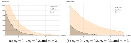
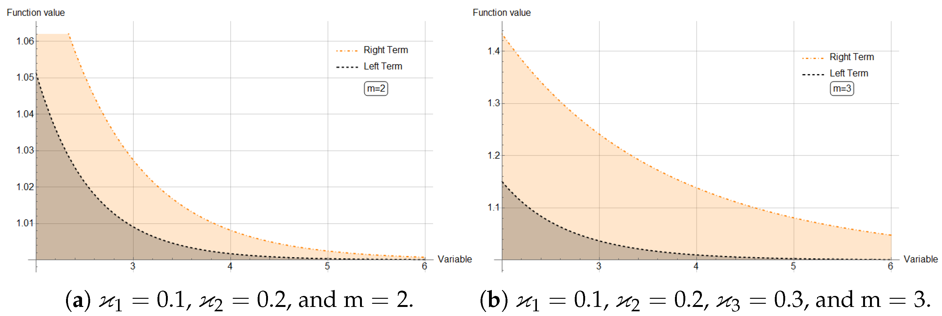
Example 2.

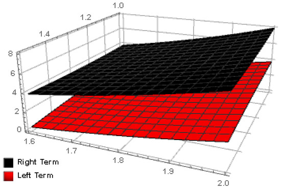
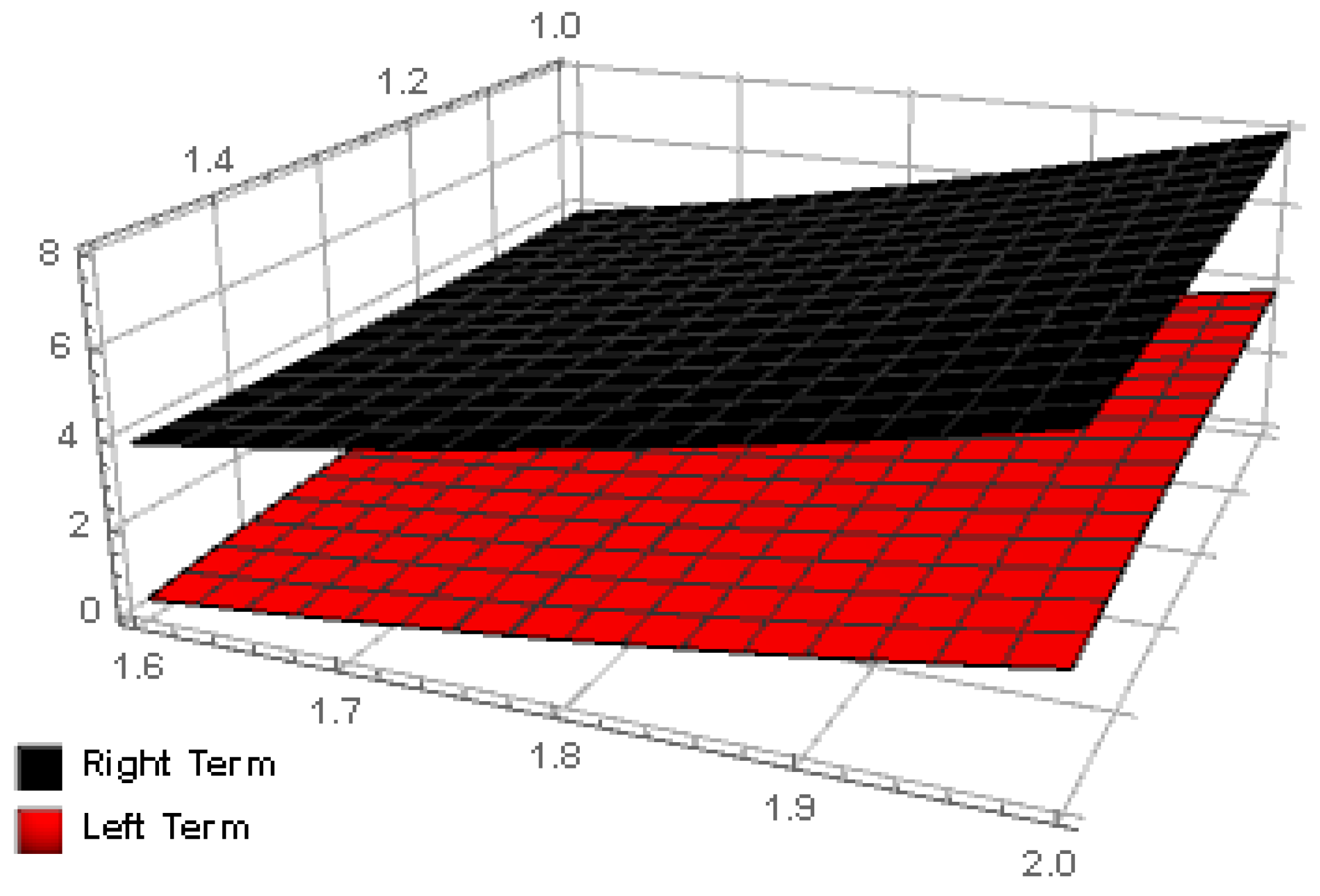
The function $\mathrm{{\rm Y}}\left(\varkappa \right)=exp\left\{{\varkappa }^{\mathfrak{n}}\right\}$ is multiplicatively superquadratic for $\mathfrak{n}\ge 2$ on $[0,\infty )$. We consider Theorem 4 for $\mathrm{m}=2$ and $\mathrm{m}=3$. Let $\mathrm{m}=2$, and we take ${\varkappa }_1=0.1$ and ${\varkappa }_2=0.2$. For $\mathrm{m}=3$, we take ${\varkappa }_1=0.1$, ${\varkappa }_2=0.2$, and ${\varkappa }_3=0.3$.

The graphical illustrations given by Figure 1 indicates a direct proportional relationship between the parameter $\mathrm{m}$ and the separation between the left and right terms of Theorem 4.

3. Midpoint-Type Inequalities for Multiplicatively Superquadratic Function

This section begins by deriving a new identity for ${}^{\ast }\mathrm{integrable}$ superquadratic functions. By employing this identity in conjunction with the Petrovič inequality, we derive novel midpoint-type inequalities for this class of functions within the framework of multiplicative calculus.

Lemma 4.

Let $\mathrm{{\rm Y}}:[0,\infty )\to (0,\infty )$ be an increasing and ${}^{\ast }\mathit{differentiable}$ function. If ${\mathrm{{\rm Y}}}^{\ast }$ is ${}^{\ast }\mathit{integrable}$, then

$$\begin{array}{ll}& {\left({\int }_0^{{\displaystyle \frac{1}{2}}}{\left({\left({\mathrm{{\rm Y}}}^{\ast }\left(\upsilon \gamma +(1-\gamma )\vartheta \right){\mathrm{{\rm Y}}}^{\ast }\left({\displaystyle \frac{\vartheta +\upsilon }{2}}-(\upsilon \gamma +(1-\gamma )\vartheta )\right)\right)}^{\gamma }\right)}^{d\gamma }\right)}^{\upsilon -\vartheta }\\ & \times {\left({\int }_{{\displaystyle \frac{1}{2}}}^1{\left({\left({\displaystyle \frac{{\mathrm{{\rm Y}}}^{\ast }\left(\upsilon \gamma +(1-\gamma )\vartheta \right)}{{\mathrm{{\rm Y}}}^{\ast }\left((\upsilon \gamma +(1-\gamma )\vartheta )-\frac{\vartheta +\upsilon }{2}\right)}}\right)}^{\gamma -1}\right)}^{d\gamma }\right)}^{\upsilon -\vartheta }\mathrm{{\rm Y}}\left(0\right)\\ & =\mathrm{{\rm Y}}\left({\displaystyle \frac{\vartheta +\upsilon }{2}}\right){\left({\int }_{\vartheta }^{\upsilon }{\left({\displaystyle \frac{\mathrm{{\rm Y}}\left(\left|\varkappa -\frac{\vartheta +\upsilon }{2}\right|\right)}{\mathrm{{\rm Y}}\left(\varkappa \right)}}\right)}^{d\varkappa }\right)}^{{\displaystyle \frac{1}{\upsilon -\vartheta }}},\end{array}$$

(20)

holds for all $\vartheta ,\upsilon \in [0,\infty )$ with $0\le \vartheta <\upsilon$.

Proof. 

The following identities can be readily derived by employing the properties established in Proposition 1 together with the ${}^{\ast }\mathrm{integration}$ by parts formula stated in Theorem 3.

$$\begin{array}{ll}& {\mathrm{I}}_1={\left({\int }_0^{{\displaystyle \frac{1}{2}}}{\left({\left({\mathrm{{\rm Y}}}^{\ast }\left(\upsilon \gamma +(1-\gamma )\vartheta \right){\mathrm{{\rm Y}}}^{\ast }\left({\displaystyle \frac{\vartheta +\upsilon }{2}}-(\upsilon \gamma +(1-\gamma )\vartheta )\right)\right)}^{\gamma }\right)}^{d\gamma }\right)}^{\upsilon -\vartheta }\\ & ={\left({\int }_0^{{\displaystyle \frac{1}{2}}}{\left({\left({\mathrm{{\rm Y}}}^{\ast }\left(\upsilon \gamma +(1-\gamma )\vartheta \right)\right)}^{\gamma }\right)}^{d\gamma }\right)}^{\upsilon -\vartheta }{\left({\int }_0^{{\displaystyle \frac{1}{2}}}{\left({\left({\mathrm{{\rm Y}}}^{\ast }\left({\displaystyle \frac{\vartheta +\upsilon }{2}}-(\upsilon \gamma +(1-\gamma )\vartheta )\right)\right)}^{\gamma }\right)}^{d\gamma }\right)}^{\upsilon -\vartheta }\\ & ={\displaystyle \frac{\sqrt{\mathrm{{\rm Y}}\left(\frac{\vartheta +\upsilon }{2}\right)}}{{\int }_0^{\frac{1}{2}}{\left(\mathrm{{\rm Y}}\left(\upsilon \gamma +(1-\gamma )\vartheta \right)\right)}^{d\gamma }}}·{\displaystyle \frac{{\int }_0^{\frac{1}{2}}{\left(\mathrm{{\rm Y}}\left(\frac{\vartheta +\upsilon }{2}-(\upsilon \gamma +(1-\gamma )\vartheta )\right)\right)}^{d\gamma }}{\sqrt{\mathrm{{\rm Y}}\left(0\right)}}}.\end{array}$$

and

$$\begin{array}{ll}& {\mathrm{I}}_2={\left({\int }_{{\displaystyle \frac{1}{2}}}^1{\left({\left({\displaystyle \frac{{\mathrm{{\rm Y}}}^{\ast }\left(\upsilon \gamma +(1-\gamma )\vartheta \right)}{{\mathrm{{\rm Y}}}^{\ast }\left((\upsilon \gamma +(1-\gamma )\vartheta )-\frac{\vartheta +\upsilon }{2}\right)}}\right)}^{\gamma -1}\right)}^{d\gamma }\right)}^{\upsilon -\vartheta }\\ & ={\displaystyle \frac{{\left({\int }_{\frac{1}{2}}^1{\left({\left({\mathrm{{\rm Y}}}^{\ast }\left(\upsilon \gamma +(1-\gamma )\vartheta \right)\right)}^{\gamma -1}\right)}^{d\gamma }\right)}^{\upsilon -\vartheta }}{{\left({\int }_{\frac{1}{2}}^1{\left({\left({\mathrm{{\rm Y}}}^{\ast }\left((\upsilon \gamma +(1-\gamma )\vartheta )-\frac{\vartheta +\upsilon }{2}\right)\right)}^{\gamma -1}\right)}^{d\gamma }\right)}^{\upsilon -\vartheta }}}\\ & ={\displaystyle \frac{\sqrt{\mathrm{{\rm Y}}\left(\frac{\vartheta +\upsilon }{2}\right)}}{{\int }_{\frac{1}{2}}^1{\left(\mathrm{{\rm Y}}\left(\upsilon \gamma +(1-\gamma )\vartheta \right)\right)}^{d\gamma }}}·{\displaystyle \frac{{\int }_{\frac{1}{2}}^1{\left(\mathrm{{\rm Y}}\left((\upsilon \gamma +(1-\gamma )\vartheta )-\frac{\vartheta +\upsilon }{2}\right)\right)}^{d\gamma }}{\sqrt{\mathrm{{\rm Y}}\left(0\right)}}}.\end{array}$$

By multiplying ${\mathrm{I}}_1$ and ${\mathrm{I}}_2$, we obtain

$$\begin{array}{ll}& {\mathrm{I}}_1\times {\mathrm{I}}_2={\displaystyle \frac{\mathrm{{\rm Y}}\left(\frac{\vartheta +\upsilon }{2}\right)}{{\int }_0^{\frac{1}{2}}{\left(\mathrm{{\rm Y}}\left(\upsilon \gamma +(1-\gamma )\vartheta \right)\right)}^{d\gamma }·{\int }_{\frac{1}{2}}^1{\left(\mathrm{{\rm Y}}\left(\upsilon \gamma +(1-\gamma )\vartheta \right)\right)}^{d\gamma }}}\\ & \times {\displaystyle \frac{{\int }_0^{\frac{1}{2}}{\left(\mathrm{{\rm Y}}\left(\frac{\vartheta +\upsilon }{2}-(\upsilon \gamma +(1-\gamma )\vartheta )\right)\right)}^{d\gamma }·{\int }_{\frac{1}{2}}^1{\left(\mathrm{{\rm Y}}\left((\upsilon \gamma +(1-\gamma )\vartheta )-\frac{\vartheta +\upsilon }{2}\right)\right)}^{d\gamma }}{\mathrm{{\rm Y}}\left(0\right)}}.\end{array}$$

Using property 4 of Proposition 1, we get

$$\begin{array}{ll}& {\mathrm{I}}_1\times {\mathrm{I}}_2={\displaystyle \frac{\mathrm{{\rm Y}}\left(\frac{\vartheta +\upsilon }{2}\right){\int }_0^1{\left(\mathrm{{\rm Y}}\left(\left|\frac{\vartheta +\upsilon }{2}-(\upsilon \gamma +(1-\gamma )\vartheta )\right|\right)\right)}^{d\gamma }}{\mathrm{{\rm Y}}\left(0\right){\int }_0^1{\left(\mathrm{{\rm Y}}\left(\upsilon \gamma +(1-\gamma )\vartheta \right)\right)}^{d\gamma }}}.\end{array}$$

(21)

Next, we perform a change of variables in (21), by setting $\varkappa =\upsilon \gamma +(1-\gamma )\vartheta$, which implies that $d\varkappa =(\upsilon -\vartheta )d\gamma$. Moreover, as $\gamma \to 1$, we have $\varkappa \to \upsilon$; also, as $\gamma \to 0$, we have $\varkappa \to \vartheta$; thus, we obtain

$$\begin{array}{ll}& {\mathrm{I}}_1\times {\mathrm{I}}_2={\displaystyle \frac{\mathrm{{\rm Y}}\left(\frac{\vartheta +\upsilon }{2}\right)}{\mathrm{{\rm Y}}\left(0\right)}}{\left({\displaystyle \frac{{\int }_{\vartheta }^{\upsilon }{\left(\mathrm{{\rm Y}}\left(\left|\varkappa -\frac{\vartheta +\upsilon }{2}\right|\right)\right)}^{d\varkappa }}{{\int }_{\vartheta }^{\upsilon }{\left(\mathrm{{\rm Y}}\left(\varkappa \right)\right)}^{d\varkappa }}}\right)}^{{\displaystyle \frac{1}{\upsilon -\vartheta }}}.\end{array}$$

Using property 3 of Proposition 1, we get

$$\begin{array}{ll}& {\mathrm{I}}_1\times {\mathrm{I}}_2={\displaystyle \frac{\mathrm{{\rm Y}}\left(\frac{\vartheta +\upsilon }{2}\right)}{\mathrm{{\rm Y}}\left(0\right)}}{\left({\int }_{\vartheta }^{\upsilon }{\left({\displaystyle \frac{\mathrm{{\rm Y}}\left(\left|\varkappa -\frac{\vartheta +\upsilon }{2}\right|\right)}{\mathrm{{\rm Y}}\left(\varkappa \right)}}\right)}^{d\varkappa }\right)}^{{\displaystyle \frac{1}{\upsilon -\vartheta }}}.\end{array}$$

This completes the proof. □

Theorem 5.

Let $\mathrm{{\rm Y}}:[0,\infty )\to (0,\infty )$ be an increasing and ${}^{\ast }\mathit{differentiable}$ multiplicatively superquadratic function. If ${\mathrm{{\rm Y}}}^{\ast }$ is increasing and ${}^{\ast }\mathit{integrable}$ and $|{\mathrm{{\rm Y}}}^{\ast }|$ is a multiplicatively superquadratic function, then

$$\begin{array}{ll}& \left|\mathrm{{\rm Y}}\left({\displaystyle \frac{\vartheta +\upsilon }{2}}\right){\left({\int }_{\vartheta }^{\upsilon }{\left({\displaystyle \frac{\mathrm{{\rm Y}}\left(\left|\varkappa -\frac{\vartheta +\upsilon }{2}\right|\right)}{\mathrm{{\rm Y}}\left(\varkappa \right)}}\right)}^{d\varkappa }\right)}^{{\displaystyle \frac{1}{\upsilon -\vartheta }}}\right|\\ & \le {\left({\left({\mathrm{{\rm Y}}}^{\ast }\left(\vartheta \right)\left({\mathrm{{\rm Y}}}^{\ast }\left(\upsilon \right)\right)\right)}^{{\displaystyle \frac{1}{2}}}{\mathrm{{\rm Y}}}^{\ast }\left({\displaystyle \frac{3\upsilon -\vartheta }{2}}\right){\left({\mathrm{{\rm Y}}}^{\ast }\left(0\right)\right)}^2\right)}^{{\displaystyle \frac{\upsilon -\vartheta }{8}}}\mathrm{{\rm Y}}\left(0\right),\end{array}$$

(22)

holds for all $\vartheta ,\upsilon \in [0,\infty )$ with $0\le \vartheta <\upsilon$.

Proof. 

Applying Lemma 4 and then taking absolute values on both sides of (20) yields

$$\begin{array}{ll}& \left|\mathrm{{\rm Y}}\left({\displaystyle \frac{\vartheta +\upsilon }{2}}\right){\left({\int }_{\vartheta }^{\upsilon }{\left({\displaystyle \frac{\mathrm{{\rm Y}}\left(\left|\varkappa -\frac{\vartheta +\upsilon }{2}\right|\right)}{\mathrm{{\rm Y}}\left(\varkappa \right)}}\right)}^{d\varkappa }\right)}^{{\displaystyle \frac{1}{\upsilon -\vartheta }}}\right|{\displaystyle \frac{1}{\mathrm{{\rm Y}}\left(0\right)}}\\ & \le exp\left\{\left(\upsilon -\vartheta \right)\left({\int }_0^{{\displaystyle \frac{1}{2}}}\gamma \left(\left|ln\left({\mathrm{{\rm Y}}}^{\ast }\left(\upsilon \gamma +(1-\gamma )\vartheta \right){\mathrm{{\rm Y}}}^{\ast }\left({\displaystyle \frac{\vartheta +\upsilon }{2}}-(\upsilon \gamma +(1-\gamma )\vartheta )\right)\right)\right|\right)d\gamma \right)\right\}\\ & \times exp\left\{\left(\upsilon -\vartheta \right)\left({\int }_{{\displaystyle \frac{1}{2}}}^1(1-\gamma )\left(\left|ln\left({\mathrm{{\rm Y}}}^{\ast }\left(\upsilon \gamma +(1-\gamma )\vartheta \right){\mathrm{{\rm Y}}}^{\ast }\left((\upsilon \gamma +(1-\gamma )\vartheta )-{\displaystyle \frac{\vartheta +\upsilon }{2}}\right)\right)\right|\right)d\gamma \right)\right\}.\end{array}$$

(23)

Since $|{\mathrm{{\rm Y}}}^{\ast }|$ is multiplicatively superquadratic, an application of Petrovič’s inequality for multiplicatively superquadratic functions (see Theorem 4) yields

$$\begin{array}{ll}& {\mathrm{{\rm Y}}}^{\ast }\left(\upsilon \gamma +(1-\gamma )\vartheta \right){\mathrm{{\rm Y}}}^{\ast }\left({\displaystyle \frac{\vartheta +\upsilon }{2}}-(\upsilon \gamma +(1-\gamma )\vartheta )\right)\\ & \le {\mathrm{{\rm Y}}}^{\ast }\left(\upsilon \gamma +(1-\gamma )\vartheta +{\displaystyle \frac{\vartheta +\upsilon }{2}}-(\upsilon \gamma +(1-\gamma )\vartheta )\right){\mathrm{{\rm Y}}}^{\ast }\left(0\right)\\ & ={\mathrm{{\rm Y}}}^{\ast }\left({\displaystyle \frac{\vartheta +\upsilon }{2}}\right){\mathrm{{\rm Y}}}^{\ast }\left(0\right)\le {\left({\mathrm{{\rm Y}}}^{\ast }\left(\vartheta \right){\mathrm{{\rm Y}}}^{\ast }\left(\upsilon \right)\right)}^{{\displaystyle \frac{1}{2}}}{\mathrm{{\rm Y}}}^{\ast }\left(0\right).\end{array}$$

(24)

Similarly, employing Petrovič’s inequality and then using the monotonicity property, we have

$$\begin{array}{ll}& {\mathrm{{\rm Y}}}^{\ast }\left(\upsilon \gamma +(1-\gamma )\vartheta \right){\mathrm{{\rm Y}}}^{\ast }\left((\upsilon \gamma +(1-\gamma )\vartheta )-{\displaystyle \frac{\vartheta +\upsilon }{2}}\right)\\ & \le {\mathrm{{\rm Y}}}^{\ast }\left(\upsilon \gamma +(1-\gamma )\vartheta +(\upsilon \gamma +(1-\gamma )\vartheta )-{\displaystyle \frac{\vartheta +\upsilon }{2}}\right){\mathrm{{\rm Y}}}^{\ast }\left(0\right)\\ & ={\mathrm{{\rm Y}}}^{\ast }\left(\left(2\gamma -{\displaystyle \frac{1}{2}}\right)\upsilon +\left({\displaystyle \frac{3}{2}}-2\gamma \right)\vartheta \right){\mathrm{{\rm Y}}}^{\ast }\left(0\right)\le {\mathrm{{\rm Y}}}^{\ast }\left({\displaystyle \frac{3\upsilon -\vartheta }{2}}\right){\mathrm{{\rm Y}}}^{\ast }\left(0\right).\end{array}$$

(25)

Substitution of the values of the results (24) and (25) into (23) yields

$$\begin{array}{ll}& \left|\mathrm{{\rm Y}}\left({\displaystyle \frac{\vartheta +\upsilon }{2}}\right){\left({\int }_{\vartheta }^{\upsilon }{\left({\displaystyle \frac{\mathrm{{\rm Y}}\left(\left|\varkappa -\frac{\vartheta +\upsilon }{2}\right|\right)}{\mathrm{{\rm Y}}\left(\varkappa \right)}}\right)}^{d\varkappa }\right)}^{{\displaystyle \frac{1}{\upsilon -\vartheta }}}\right|{\displaystyle \frac{1}{\mathrm{{\rm Y}}\left(0\right)}}\\ & \le exp\left\{\left(\upsilon -\vartheta \right)\left({\int }_0^{{\displaystyle \frac{1}{2}}}\gamma \left(\left|ln\left({\left({\mathrm{{\rm Y}}}^{\ast }\left(\vartheta \right){\mathrm{{\rm Y}}}^{\ast }\left(\upsilon \right)\right)}^{{\displaystyle \frac{1}{2}}}{\mathrm{{\rm Y}}}^{\ast }\left(0\right)\right)\right|\right)d\gamma \right)\right\}\\ & \times exp\left\{\left(\upsilon -\vartheta \right)\left({\int }_{{\displaystyle \frac{1}{2}}}^1(1-\gamma )\left(\left|ln\left({\mathrm{{\rm Y}}}^{\ast }\left({\displaystyle \frac{3\upsilon -\vartheta }{2}}\right){\mathrm{{\rm Y}}}^{\ast }\left(0\right)\right)\right|\right)d\gamma \right)\right\}.\end{array}$$

Using properties of logarithm and then employing the Riemann integration with regard to γ, we obtain

$$\begin{array}{ll}& \left|\mathrm{{\rm Y}}\left({\displaystyle \frac{\vartheta +\upsilon }{2}}\right){\left({\int }_{\vartheta }^{\upsilon }{\left({\displaystyle \frac{\mathrm{{\rm Y}}\left(\left|\varkappa -\frac{\vartheta +\upsilon }{2}\right|\right)}{\mathrm{{\rm Y}}\left(\varkappa \right)}}\right)}^{d\varkappa }\right)}^{{\displaystyle \frac{1}{\upsilon -\vartheta }}}\right|{\displaystyle \frac{1}{\mathrm{{\rm Y}}\left(0\right)}}\\ & \le exp\left\{{\displaystyle \frac{\left(\upsilon -\vartheta \right)\left(\left|ln\left({\left({\mathrm{{\rm Y}}}^{\ast }\left(\vartheta \right){\mathrm{{\rm Y}}}^{\ast }\left(\upsilon \right)\right)}^{\frac{1}{2}}{\mathrm{{\rm Y}}}^{\ast }\left(0\right)\right)\right|\right)}{8}}\right\}\\ & \times exp\left\{{\displaystyle \frac{\left(\upsilon -\vartheta \right)\left|ln\left({\mathrm{{\rm Y}}}^{\ast }\left(\frac{3\upsilon -\vartheta }{2}\right){\mathrm{{\rm Y}}}^{\ast }\left(0\right)\right|\right)}{8}}\right\}\\ & =exp\left\{{\displaystyle \frac{\left(\upsilon -\vartheta \right)}{8}}ln\left({\left({\mathrm{{\rm Y}}}^{\ast }\left(\vartheta \right){\mathrm{{\rm Y}}}^{\ast }\left(\upsilon \right)\right)}^{{\displaystyle \frac{1}{2}}}{\mathrm{{\rm Y}}}^{\ast }\left({\displaystyle \frac{3\upsilon -\vartheta }{2}}\right){\left({\mathrm{{\rm Y}}}^{\ast }\left(0\right)\right)}^2\right)\right\}\\ & ={\left({\left({\mathrm{{\rm Y}}}^{\ast }\left(\vartheta \right)\left({\mathrm{{\rm Y}}}^{\ast }\left(\upsilon \right)\right)\right)}^{{\displaystyle \frac{1}{2}}}{\mathrm{{\rm Y}}}^{\ast }\left({\displaystyle \frac{3\upsilon -\vartheta }{2}}\right){\left({\mathrm{{\rm Y}}}^{\ast }\left(0\right)\right)}^2\right)}^{{\displaystyle \frac{\upsilon -\vartheta }{8}}}.\end{array}$$

This completes the proof. □

Theorem 6.

Let $\mathrm{{\rm Y}}:[0,\infty )\to (0,\infty )$ be an increasing and ${}^{\ast }\mathit{differentiable}$ multiplicatively superquadratic function. If ${\mathrm{{\rm Y}}}^{\ast }$ is ${}^{\ast }\mathit{integrable}$ and $|ln\left({\mathrm{{\rm Y}}}^{\ast }\right){|}^{\mathrm{p}}$ is a superquadratic function, then

$$\begin{array}{ll}& \left|\mathrm{{\rm Y}}\left({\displaystyle \frac{\vartheta +\upsilon }{2}}\right){\left({\int }_{\vartheta }^{\upsilon }{\left({\displaystyle \frac{\mathrm{{\rm Y}}\left(\left|\varkappa -\frac{\vartheta +\upsilon }{2}\right|\right)}{\mathrm{{\rm Y}}\left(\varkappa \right)}}\right)}^{d\varkappa }\right)}^{{\displaystyle \frac{1}{\upsilon -\vartheta }}}\right|\\ & \le {\left[{\left({\mathrm{{\rm Y}}}^{\ast }\left(\upsilon \right){\mathrm{{\rm Y}}}^{\ast }\left(\vartheta \right)\right)}^{\left({\displaystyle \frac{1+3^{\frac{1}{\mathrm{p}}}}{2^{1+\frac{1}{\mathrm{p}}}}}\right)}{\mathrm{{\rm Y}}}^{\ast }\left({\displaystyle \frac{\upsilon -\vartheta }{2}}\right){\mathrm{{\rm Y}}}^{\ast }\left(0\right)\right]}^{{\displaystyle \frac{\left(\upsilon -\vartheta \right)}{2^{1+\frac{1}{\mathrm{p}}}{(\mathrm{q}+1)}^{\frac{1}{\mathrm{q}}}}}},\end{array}$$

(26)

holds for all $\vartheta ,\upsilon \in [0,\infty )$ with $0\le \vartheta <\upsilon$. Where $\mathrm{q}>1$, ${\displaystyle \frac{1}{\mathrm{q}}}+{\displaystyle \frac{1}{\mathrm{p}}}=1.$

Proof. 

Applying Lemma 4 and then taking absolute values on both sides of (20) yields

$$\begin{array}{ll}& \left|\mathrm{{\rm Y}}\left({\displaystyle \frac{\vartheta +\upsilon }{2}}\right){\left({\int }_{\vartheta }^{\upsilon }{\left({\displaystyle \frac{\mathrm{{\rm Y}}\left(\left|\varkappa -\frac{\vartheta +\upsilon }{2}\right|\right)}{\mathrm{{\rm Y}}\left(\varkappa \right)}}\right)}^{d\varkappa }\right)}^{{\displaystyle \frac{1}{\upsilon -\vartheta }}}\right|{\displaystyle \frac{1}{\mathrm{{\rm Y}}\left(0\right)}}\\ & \le exp\left\{\left(\upsilon -\vartheta \right)\left({\int }_0^{{\displaystyle \frac{1}{2}}}\gamma \left(\left|ln\left({\mathrm{{\rm Y}}}^{\ast }\left(\upsilon \gamma +(1-\gamma )\vartheta \right){\mathrm{{\rm Y}}}^{\ast }\left({\displaystyle \frac{\vartheta +\upsilon }{2}}-(\upsilon \gamma +(1-\gamma )\vartheta )\right)\right)\right|\right)d\gamma \right)\right\}\\ & \times exp\left\{\left(\upsilon -\vartheta \right)\left({\int }_{{\displaystyle \frac{1}{2}}}^1(1-\gamma )\left(\left|ln\left({\mathrm{{\rm Y}}}^{\ast }\left(\upsilon \gamma +(1-\gamma )\vartheta \right){\mathrm{{\rm Y}}}^{\ast }\left((\upsilon \gamma +(1-\gamma )\vartheta )-{\displaystyle \frac{\vartheta +\upsilon }{2}}\right)\right)\right|\right)d\gamma \right)\right\}.\end{array}$$

Using Hölder inequality, we obtain

$$\begin{array}{ll}& \left|\mathrm{{\rm Y}}\left({\displaystyle \frac{\vartheta +\upsilon }{2}}\right){\left({\int }_{\vartheta }^{\upsilon }{\left({\displaystyle \frac{\mathrm{{\rm Y}}\left(\left|\varkappa -\frac{\vartheta +\upsilon }{2}\right|\right)}{\mathrm{{\rm Y}}\left(\varkappa \right)}}\right)}^{d\varkappa }\right)}^{{\displaystyle \frac{1}{\upsilon -\vartheta }}}\right|{\displaystyle \frac{1}{\mathrm{{\rm Y}}\left(0\right)}}\\ & \le exp\left\{\left(\upsilon -\vartheta \right){\left({\int }_0^{{\displaystyle \frac{1}{2}}}{\gamma }^{\mathrm{q}}d\gamma \right)}^{{\displaystyle \frac{1}{\mathrm{q}}}}{\left({\int }_0^{{\displaystyle \frac{1}{2}}}\left({\left|ln\left({\mathrm{{\rm Y}}}^{\ast }\left(\upsilon \gamma +(1-\gamma )\vartheta \right)\right)\right|}^{\mathrm{p}}\right)d\gamma \right)}^{{\displaystyle \frac{1}{\mathrm{p}}}}\right\}\\ & \times exp\left\{\left(\upsilon -\vartheta \right){\left({\int }_0^{{\displaystyle \frac{1}{2}}}{\gamma }^{\mathrm{q}}d\gamma \right)}^{{\displaystyle \frac{1}{\mathrm{q}}}}{\left({\int }_0^{{\displaystyle \frac{1}{2}}}\left({\left|ln\left({\mathrm{{\rm Y}}}^{\ast }\left({\displaystyle \frac{\vartheta +\upsilon }{2}}-(\upsilon \gamma +(1-\gamma )\vartheta )\right)\right)\right|}^{\mathrm{p}}\right)d\gamma \right)}^{{\displaystyle \frac{1}{\mathrm{p}}}}\right\}\\ & \times exp\left\{\left(\upsilon -\vartheta \right){\left({\int }_{{\displaystyle \frac{1}{2}}}^1{(1-\gamma )}^{\mathrm{q}}d\gamma \right)}^{{\displaystyle \frac{1}{\mathrm{q}}}}{\left({\int }_{{\displaystyle \frac{1}{2}}}^1\left({\left|ln\left({\mathrm{{\rm Y}}}^{\ast }\left(\upsilon \gamma +(1-\gamma )\vartheta \right)\right)\right|}^{\mathrm{p}}\right)d\gamma \right)}^{{\displaystyle \frac{1}{\mathrm{p}}}}\right\}\\ & \times exp\left\{\left(\upsilon -\vartheta \right){\left({\int }_{{\displaystyle \frac{1}{2}}}^1{(1-\gamma )}^{\mathrm{q}}d\gamma \right)}^{{\displaystyle \frac{1}{\mathrm{q}}}}{\left({\int }_{{\displaystyle \frac{1}{2}}}^1\left({\left|ln\left({\mathrm{{\rm Y}}}^{\ast }\left(\upsilon \gamma +(1-\gamma )\vartheta -{\displaystyle \frac{\vartheta +\upsilon }{2}}\right)\right)\right|}^{\mathrm{p}}\right)d\gamma \right)}^{{\displaystyle \frac{1}{\mathrm{p}}}}\right\}.\end{array}$$

Since $|ln\left({\mathrm{{\rm Y}}}^{\ast }\right){|}^{\mathrm{p}}$ is superquadratic. Moreover, noting that $|ln{\mathrm{{\rm Y}}}^{\ast }{|}^{\mathrm{p}}\ge 0$, Lemma 2 ensures that $|ln{\mathrm{{\rm Y}}}^{\ast }{|}^{\mathrm{p}}$ is a convex function. Therefore, by invoking the definition of convexity together with the classical Hermite–Hadamard-type inequality for convex functions, we obtain

$$\begin{array}{ll}& \left|\mathrm{{\rm Y}}\left({\displaystyle \frac{\vartheta +\upsilon }{2}}\right){\left({\int }_{\vartheta }^{\upsilon }{\left({\displaystyle \frac{\mathrm{{\rm Y}}\left(\left|\varkappa -\frac{\vartheta +\upsilon }{2}\right|\right)}{\mathrm{{\rm Y}}\left(\varkappa \right)}}\right)}^{d\varkappa }\right)}^{{\displaystyle \frac{1}{\upsilon -\vartheta }}}\right|{\displaystyle \frac{1}{\mathrm{{\rm Y}}\left(0\right)}}\\ & \le exp\left\{{\displaystyle \frac{\left(\upsilon -\vartheta \right)}{2^{\frac{1+\mathrm{q}}{\mathrm{q}}}{(\mathrm{q}+1)}^{\frac{1}{\mathrm{q}}}}}{\left({\int }_0^{{\displaystyle \frac{1}{2}}}\left(\gamma {\left|ln\left({\mathrm{{\rm Y}}}^{\ast }\left(\upsilon \right)\right)\right|}^{\mathrm{p}}+(1-\gamma ){\left|ln\left({\mathrm{{\rm Y}}}^{\ast }\left(\vartheta \right)\right)\right|}^{\mathrm{p}}\right)d\gamma \right)}^{{\displaystyle \frac{1}{\mathrm{p}}}}\right\}\\ & \times exp\left\{{\displaystyle \frac{\left(\upsilon -\vartheta \right)}{2^{\frac{1+\mathrm{q}}{\mathrm{q}}}{(\mathrm{q}+1)}^{\frac{1}{\mathrm{q}}}}}{\left({\displaystyle \frac{{\left|ln\left({\mathrm{{\rm Y}}}^{\ast }\left(0\right)\right)\right|}^{\mathrm{p}}+{\left|ln\left({\mathrm{{\rm Y}}}^{\ast }\left(\frac{\upsilon -\vartheta }{2}\right)\right)\right|}^{\mathrm{p}}}{4}}\right)}^{{\displaystyle \frac{1}{\mathrm{p}}}}\right\}\\ & \times exp\left\{{\displaystyle \frac{\left(\upsilon -\vartheta \right)}{2^{\frac{1+\mathrm{q}}{\mathrm{q}}}{(\mathrm{q}+1)}^{\frac{1}{\mathrm{q}}}}}{\left({\int }_{{\displaystyle \frac{1}{2}}}^1\left(\gamma {\left|ln\left({\mathrm{{\rm Y}}}^{\ast }\left(\upsilon \right)\right)\right|}^{\mathrm{p}}+(1-\gamma ){\left|ln\left({\mathrm{{\rm Y}}}^{\ast }\left(\vartheta \right)\right)\right|}^{\mathrm{p}}\right)d\gamma \right)}^{{\displaystyle \frac{1}{\mathrm{p}}}}\right\}\\ & \times exp\left\{{\displaystyle \frac{\left(\upsilon -\vartheta \right)}{2^{\frac{1+\mathrm{q}}{\mathrm{q}}}{(\mathrm{q}+1)}^{\frac{1}{\mathrm{q}}}}}{\left({\displaystyle \frac{{\left|ln\left({\mathrm{{\rm Y}}}^{\ast }\left(0\right)\right)\right|}^{\mathrm{p}}+{\left|ln\left({\mathrm{{\rm Y}}}^{\ast }\left(\frac{\upsilon -\vartheta }{2}\right)\right)\right|}^{\mathrm{p}}}{4}}\right)}^{{\displaystyle \frac{1}{\mathrm{p}}}}\right\}\\ & =exp\left\{{\displaystyle \frac{\left(\upsilon -\vartheta \right)}{2^{\frac{1+\mathrm{q}}{\mathrm{q}}}{(\mathrm{q}+1)}^{\frac{1}{\mathrm{q}}}}}{\left({\displaystyle \frac{{\left|ln\left({\mathrm{{\rm Y}}}^{\ast }\left(\upsilon \right)\right)\right|}^{\mathrm{p}}+3{\left|ln\left({\mathrm{{\rm Y}}}^{\ast }\left(\vartheta \right)\right)\right|}^{\mathrm{p}}}{8}}\right)}^{{\displaystyle \frac{1}{\mathrm{p}}}}\right\}\\ & \times exp\left\{{\displaystyle \frac{2\left(\upsilon -\vartheta \right)}{2^{\frac{1+\mathrm{q}}{\mathrm{q}}}{(\mathrm{q}+1)}^{\frac{1}{\mathrm{q}}}}}{\left({\displaystyle \frac{{\left|ln\left({\mathrm{{\rm Y}}}^{\ast }\left(0\right)\right)\right|}^{\mathrm{p}}+{\left|ln\left({\mathrm{{\rm Y}}}^{\ast }\left(\frac{\upsilon -\vartheta }{2}\right)\right)\right|}^{\mathrm{p}}}{4}}\right)}^{{\displaystyle \frac{1}{\mathrm{p}}}}\right\}\\ & \times exp\left\{{\displaystyle \frac{\left(\upsilon -\vartheta \right)}{2^{\frac{1+\mathrm{q}}{\mathrm{q}}}{(\mathrm{q}+1)}^{\frac{1}{\mathrm{q}}}}}{\left({\displaystyle \frac{3{\left|ln\left({\mathrm{{\rm Y}}}^{\ast }\left(\upsilon \right)\right)\right|}^{\mathrm{p}}+{\left|ln\left({\mathrm{{\rm Y}}}^{\ast }\left(\vartheta \right)\right)\right|}^{\mathrm{p}}}{8}}\right)}^{{\displaystyle \frac{1}{\mathrm{p}}}}\right\}.\end{array}$$

This further implies that

$$\begin{array}{ll}& \left|\mathrm{{\rm Y}}\left({\displaystyle \frac{\vartheta +\upsilon }{2}}\right){\left({\int }_{\vartheta }^{\upsilon }{\left({\displaystyle \frac{\mathrm{{\rm Y}}\left(\left|\varkappa -\frac{\vartheta +\upsilon }{2}\right|\right)}{\mathrm{{\rm Y}}\left(\varkappa \right)}}\right)}^{d\varkappa }\right)}^{{\displaystyle \frac{1}{\upsilon -\vartheta }}}\right|{\displaystyle \frac{1}{\mathrm{{\rm Y}}\left(0\right)}}\\ & \le exp\left\{{\displaystyle \frac{\left(\upsilon -\vartheta \right)}{2^{2(1+\frac{1}{\mathrm{p}})}{(\mathrm{q}+1)}^{\frac{1}{\mathrm{q}}}}}\left[{\left({\left|ln\left({\mathrm{{\rm Y}}}^{\ast }\left(\upsilon \right)\right)\right|}^{\mathrm{p}}+3{\left|ln\left({\mathrm{{\rm Y}}}^{\ast }\left(\vartheta \right)\right)\right|}^{\mathrm{p}}\right)}^{{\displaystyle \frac{1}{\mathrm{p}}}}+{\left(3{\left|ln\left({\mathrm{{\rm Y}}}^{\ast }\left(\upsilon \right)\right)\right|}^{\mathrm{p}}+{\left|ln\left({\mathrm{{\rm Y}}}^{\ast }\left(\vartheta \right)\right)\right|}^{\mathrm{p}}\right)}^{{\displaystyle \frac{1}{\mathrm{p}}}}\right]\right\}\\ & \times exp\left\{{\displaystyle \frac{\left(\upsilon -\vartheta \right)}{2^{1+\frac{1}{\mathrm{p}}}{(\mathrm{q}+1)}^{\frac{1}{\mathrm{q}}}}}{\left({\left|ln\left({\mathrm{{\rm Y}}}^{\ast }\left(0\right)\right)\right|}^{\mathrm{p}}+{\left|ln\left({\mathrm{{\rm Y}}}^{\ast }\left({\displaystyle \frac{\upsilon -\vartheta }{2}}\right)\right)\right|}^{\mathrm{p}}\right)}^{{\displaystyle \frac{1}{\mathrm{p}}}}\right\}.\end{array}$$

(27)

Since $ln{\mathrm{{\rm Y}}}^{\ast }\left(\varkappa \right)\ge 0$, it follows that $|ln{\mathrm{{\rm Y}}}^{\ast }\left(\varkappa \right)|=ln{\mathrm{{\rm Y}}}^{\ast }\left(\varkappa \right)$. Using this observation, we can further simplify (27) by applying the inequality ${(\vartheta +\upsilon )}^{\mathrm{s}}\le {\vartheta }^{\mathrm{s}}+{\upsilon }^{\mathrm{s}},\forall \mathrm{s}\in [0,1).$

$$\begin{array}{ll}& \left|\mathrm{{\rm Y}}\left({\displaystyle \frac{\vartheta +\upsilon }{2}}\right){\left({\int }_{\vartheta }^{\upsilon }{\left({\displaystyle \frac{\mathrm{{\rm Y}}\left(\left|\varkappa -\frac{\vartheta +\upsilon }{2}\right|\right)}{\mathrm{{\rm Y}}\left(\varkappa \right)}}\right)}^{d\varkappa }\right)}^{{\displaystyle \frac{1}{\upsilon -\vartheta }}}\right|{\displaystyle \frac{1}{\mathrm{{\rm Y}}\left(0\right)}}\\ & \le exp\left\{{\displaystyle \frac{\left(\upsilon -\vartheta \right)}{2^{2(1+\frac{1}{\mathrm{p}})}{(\mathrm{q}+1)}^{\frac{1}{\mathrm{q}}}}}\left[ln\left({\mathrm{{\rm Y}}}^{\ast }\left(\upsilon \right)\right)+3^{{\displaystyle \frac{1}{\mathrm{p}}}}ln\left({\mathrm{{\rm Y}}}^{\ast }\left(\vartheta \right)\right)+3^{{\displaystyle \frac{1}{\mathrm{p}}}}ln\left({\mathrm{{\rm Y}}}^{\ast }\left(\upsilon \right)\right)+ln\left({\mathrm{{\rm Y}}}^{\ast }\left(\vartheta \right)\right)\right]\right\}\\ & \times exp\left\{{\displaystyle \frac{\left(\upsilon -\vartheta \right)}{2^{1+\frac{1}{\mathrm{p}}}{(\mathrm{q}+1)}^{\frac{1}{\mathrm{q}}}}}\left(ln\left({\mathrm{{\rm Y}}}^{\ast }\left(0\right)\right)+ln\left({\mathrm{{\rm Y}}}^{\ast }\left({\displaystyle \frac{\upsilon -\vartheta }{2}}\right)\right)\right)\right\}\\ & =exp\left\{{\displaystyle \frac{(1+3^{\frac{1}{\mathrm{p}}})\left(\upsilon -\vartheta \right)}{2^{2(1+\frac{1}{\mathrm{p}})}{(\mathrm{q}+1)}^{\frac{1}{\mathrm{q}}}}}\left[ln\left({\mathrm{{\rm Y}}}^{\ast }\left(\upsilon \right){\mathrm{{\rm Y}}}^{\ast }\left(\vartheta \right)\right)\right]\right\}\\ & \times exp\left\{{\displaystyle \frac{\left(\upsilon -\vartheta \right)}{2^{1+\frac{1}{\mathrm{p}}}{(\mathrm{q}+1)}^{\frac{1}{\mathrm{q}}}}}\left[ln\left({\mathrm{{\rm Y}}}^{\ast }\left(0\right){\mathrm{{\rm Y}}}^{\ast }\left({\displaystyle \frac{\upsilon -\vartheta }{2}}\right)\right)\right]\right\}\\ & =exp\left\{ln{\left[{\left({\mathrm{{\rm Y}}}^{\ast }\left(\upsilon \right){\mathrm{{\rm Y}}}^{\ast }\left(\vartheta \right)\right)}^{\left({\displaystyle \frac{1+3^{\frac{1}{\mathrm{p}}}}{2^{1+\frac{1}{\mathrm{p}}}}}\right)}\left({\mathrm{{\rm Y}}}^{\ast }\left(0\right){\mathrm{{\rm Y}}}^{\ast }\left({\displaystyle \frac{\upsilon -\vartheta }{2}}\right)\right)\right]}^{{\displaystyle \frac{\left(\upsilon -\vartheta \right)}{2^{1+\frac{1}{\mathrm{p}}}{(\mathrm{q}+1)}^{\frac{1}{\mathrm{q}}}}}}\right\}\\ & ={\left[{\left({\mathrm{{\rm Y}}}^{\ast }\left(\upsilon \right){\mathrm{{\rm Y}}}^{\ast }\left(\vartheta \right)\right)}^{\left({\displaystyle \frac{1+3^{\frac{1}{\mathrm{p}}}}{2^{1+\frac{1}{\mathrm{p}}}}}\right)}\left({\mathrm{{\rm Y}}}^{\ast }\left(0\right){\mathrm{{\rm Y}}}^{\ast }\left({\displaystyle \frac{\upsilon -\vartheta }{2}}\right)\right)\right]}^{{\displaystyle \frac{\left(\upsilon -\vartheta \right)}{2^{1+\frac{1}{\mathrm{p}}}{(\mathrm{q}+1)}^{\frac{1}{\mathrm{q}}}}}}.\end{array}$$

This completes the proof. □

4. Trapezoid-Type Inequalities for Multiplicatively Superquadratic Function

This section begins by deriving a new identity for ${}^{\ast }\mathrm{integrable}$ multiplicatively superquadratic functions from the perspective of multiplicative calculus. By utilizing this identity in conjunction with Petrovič’s inequality, we subsequently derive novel trapezoid-type inequalities for this class of functions.

Lemma 5.

Let $\mathrm{{\rm Y}}:[0,\infty )\to (0,\infty )$ be an increasing and ${}^{\ast }\mathit{differentiable}$ function. If ${\mathrm{{\rm Y}}}^{\ast }$ is ${}^{\ast }\mathit{integrable}$, then

$$\begin{array}{ll}& {\left({\int }_0^1{\left({\left({\mathrm{{\rm Y}}}^{\ast }\left(\upsilon \gamma +(1-\gamma )\vartheta \right)\right)}^{1-2\gamma }{\left({\mathrm{{\rm Y}}}^{\ast }\left((\upsilon -\vartheta )\gamma \right)\right)}^{{(1-\gamma )}^2}{\left({\mathrm{{\rm Y}}}^{\ast }\left((\upsilon -\vartheta )(1-\gamma )\right)\right)}^{{\gamma }^2}\right)}^{d\gamma }\right)}^{{\displaystyle \frac{\upsilon -\vartheta }{2}}}\\ & ={\displaystyle \frac{{\left({\int }_{\vartheta }^{\upsilon }{\left(\mathrm{{\rm Y}}\left(\varkappa \right){\left(\mathrm{{\rm Y}}\left(\varkappa -\vartheta \right)\right)}^{\frac{\upsilon -\varkappa }{\upsilon -\vartheta }}{\left(\mathrm{{\rm Y}}\left(\upsilon -\varkappa \right)\right)}^{\frac{\varkappa -\vartheta }{\upsilon -\vartheta }}\right)}^{d\varkappa }\right)}^{\frac{1}{\upsilon -\vartheta }}}{\left(\sqrt{\mathrm{{\rm Y}}\left(\vartheta \right)\mathrm{{\rm Y}}\left(\upsilon \right)}\right)\mathrm{{\rm Y}}\left(0\right)}},\end{array}$$

(28)

holds for all $\vartheta ,\upsilon \in [0,\infty )$ with $0\le \vartheta <\upsilon$.

Proof. 

The following identity follow directly from the properties established in Proposition 1, together with the ${}^{\ast }\mathrm{integration}$ by parts formula presented in Theorem 3.

$$\begin{array}{ll}& \mathrm{I}={\left({\int }_0^1{\left({\left({\mathrm{{\rm Y}}}^{\ast }\left(\upsilon \gamma +(1-\gamma )\vartheta \right)\right)}^{1-2\gamma }{\left({\mathrm{{\rm Y}}}^{\ast }\left((\upsilon -\vartheta )\gamma \right)\right)}^{{(1-\gamma )}^2}{\left({\mathrm{{\rm Y}}}^{\ast }\left((\upsilon -\vartheta )(1-\gamma )\right)\right)}^{{\gamma }^2}\right)}^{d\gamma }\right)}^{{\displaystyle \frac{\upsilon -\vartheta }{2}}}\\ & ={\left({\int }_0^1{\left({\left({\mathrm{{\rm Y}}}^{\ast }\left(\upsilon \gamma +(1-\gamma )\vartheta \right)\right)}^{1-2\gamma }\right)}^{d\gamma }\right)}^{{\displaystyle \frac{\upsilon -\vartheta }{2}}}{\left({\int }_0^1{\left({\left({\mathrm{{\rm Y}}}^{\ast }\left((\upsilon -\vartheta )\gamma \right)\right)}^{{(1-\gamma )}^2}\right)}^{d\gamma }\right)}^{{\displaystyle \frac{\upsilon -\vartheta }{2}}}\\ & \times {\left({\int }_0^1{\left({\left({\mathrm{{\rm Y}}}^{\ast }\left((\upsilon -\vartheta )(1-\gamma )\right)\right)}^{{\gamma }^2}\right)}^{d\gamma }\right)}^{{\displaystyle \frac{\upsilon -\vartheta }{2}}}\\ & ={\displaystyle \frac{{\int }_0^1{\left(\mathrm{{\rm Y}}\left(\upsilon \gamma +(1-\gamma )\vartheta \right)\right)}^{d\gamma }}{\sqrt{\mathrm{{\rm Y}}\left(\vartheta \right)\mathrm{{\rm Y}}\left(\upsilon \right)}}}·{\displaystyle \frac{{\int }_0^1{\left({\left(\mathrm{{\rm Y}}\left((\upsilon -\vartheta )\gamma \right)\right)}^{1-\gamma }\right)}^{d\gamma }}{\sqrt{\mathrm{{\rm Y}}\left(0\right)}}}·{\displaystyle \frac{{\int }_0^1{\left({\left(\mathrm{{\rm Y}}\left((\upsilon -\vartheta )(1-\gamma )\right)\right)}^{\gamma }\right)}^{d\gamma }}{\sqrt{\mathrm{{\rm Y}}\left(0\right)}}}\\ & ={\displaystyle \frac{{\int }_0^1{\left(\mathrm{{\rm Y}}\left(\upsilon \gamma +(1-\gamma )\vartheta \right)\right)}^{d\gamma }{\int }_0^1{\left({\left(\mathrm{{\rm Y}}\left((\upsilon -\vartheta )\gamma \right)\right)}^{1-\gamma }\right)}^{d\gamma }{\int }_0^1{\left({\left(\mathrm{{\rm Y}}\left((\upsilon -\vartheta )(1-\gamma )\right)\right)}^{\gamma }\right)}^{d\gamma }}{\left(\sqrt{\mathrm{{\rm Y}}\left(\vartheta \right)\mathrm{{\rm Y}}\left(\upsilon \right)}\right)\mathrm{{\rm Y}}\left(0\right)}}\end{array}$$

(29)

By performing a change of variables in (29), we obtain

$$\begin{array}{ll}& \mathrm{I}={\displaystyle \frac{{\left({\int }_{\vartheta }^{\upsilon }{\left(\mathrm{{\rm Y}}\left(\varkappa \right)\right)}^{d\varkappa }\right)}^{\frac{1}{\upsilon -\vartheta }}{\left({\int }_{\vartheta }^{\upsilon }{\left({\left(\mathrm{{\rm Y}}(\varkappa -\vartheta )\right)}^{\frac{\upsilon -\varkappa }{\upsilon -\vartheta }}\right)}^{d\varkappa }\right)}^{\frac{1}{\upsilon -\vartheta }}{\left({\int }_{\vartheta }^{\upsilon }{\left({\left(\mathrm{{\rm Y}}(\upsilon -\varkappa )\right)}^{\frac{\varkappa -\vartheta }{\upsilon -\vartheta }}\right)}^{d\varkappa }\right)}^{\frac{1}{\upsilon -\vartheta }}}{\left(\sqrt{\mathrm{{\rm Y}}\left(\vartheta \right)\mathrm{{\rm Y}}\left(\upsilon \right)}\right)\mathrm{{\rm Y}}\left(0\right)}}\\ & ={\displaystyle \frac{{\left({\int }_{\vartheta }^{\upsilon }{\left(\mathrm{{\rm Y}}\left(\varkappa \right){\left(\mathrm{{\rm Y}}\left(\varkappa -\vartheta \right)\right)}^{\frac{\upsilon -\varkappa }{\upsilon -\vartheta }}{\left(\mathrm{{\rm Y}}\left(\upsilon -\varkappa \right)\right)}^{\frac{\varkappa -\vartheta }{\upsilon -\vartheta }}\right)}^{d\varkappa }\right)}^{\frac{1}{\upsilon -\vartheta }}}{\left(\sqrt{\mathrm{{\rm Y}}\left(\vartheta \right)\mathrm{{\rm Y}}\left(\upsilon \right)}\right)\mathrm{{\rm Y}}\left(0\right)}}.\end{array}$$

This completes the proof. □

Theorem 7.

Let $\mathrm{{\rm Y}}:[0,\infty )\to (0,\infty )$ be an increasing and ${}^{\ast }\mathit{differentiable}$ multiplicatively superquadratic function. If ${\mathrm{{\rm Y}}}^{\ast }$ is ${}^{\ast }\mathit{integrable}$ and $|{\mathrm{{\rm Y}}}^{\ast }|$ is a multiplicatively superquadratic function, then

$$\begin{array}{ll}& \left|{\displaystyle \frac{{\left({\int }_{\vartheta }^{\upsilon }{\left(\mathrm{{\rm Y}}\left(\varkappa \right){\left(\mathrm{{\rm Y}}\left(\varkappa -\vartheta \right)\right)}^{\frac{\upsilon -\varkappa }{\upsilon -\vartheta }}{\left(\mathrm{{\rm Y}}\left(\upsilon -\varkappa \right)\right)}^{\frac{\varkappa -\vartheta }{\upsilon -\vartheta }}\right)}^{d\varkappa }\right)}^{\frac{1}{\upsilon -\vartheta }}}{\left(\sqrt{\mathrm{{\rm Y}}\left(\vartheta \right)\mathrm{{\rm Y}}\left(\upsilon \right)}\right)\mathrm{{\rm Y}}\left(0\right)}}\right|\\ & \le {\left({\left({\mathrm{{\rm Y}}}^{\ast }\left(2\upsilon -\vartheta \right)\right)}^3{\left({\mathrm{{\rm Y}}}^{\ast }\left(\upsilon -\vartheta \right)\right)}^2{\left({\mathrm{{\rm Y}}}^{\ast }\left(0\right)\right)}^5\right)}^{{\displaystyle \frac{\upsilon -\vartheta }{12}}},\end{array}$$

(30)

holds for all $\vartheta ,\upsilon \in [0,\infty )$ with $0\le \vartheta <\upsilon$.

Proof. 

Applying Lemma 5 and then taking absolute values on both sides of (28) yields

$$\begin{array}{ll}& \left|{\displaystyle \frac{{\left({\int }_{\vartheta }^{\upsilon }{\left(\mathrm{{\rm Y}}\left(\varkappa \right){\left(\mathrm{{\rm Y}}\left(\varkappa -\vartheta \right)\right)}^{\frac{\upsilon -\varkappa }{\upsilon -\vartheta }}{\left(\mathrm{{\rm Y}}\left(\upsilon -\varkappa \right)\right)}^{\frac{\varkappa -\vartheta }{\upsilon -\vartheta }}\right)}^{d\varkappa }\right)}^{\frac{1}{\upsilon -\vartheta }}}{\left(\sqrt{\mathrm{{\rm Y}}\left(\vartheta \right)\mathrm{{\rm Y}}\left(\upsilon \right)}\right)\mathrm{{\rm Y}}\left(0\right)}}\right|\\ & \le exp\left\{{\displaystyle \frac{\upsilon -\vartheta }{2}}\left({\int }_0^1\left|1-2\gamma \right|\left|ln{\mathrm{{\rm Y}}}^{\ast }\left(\upsilon \gamma +(1-\gamma )\vartheta \right)\right|d\gamma \right)\right\}\\ & \times exp\left\{{\displaystyle \frac{\upsilon -\vartheta }{2}}\left({\int }_0^1{\left(1-\gamma \right)}^2\left|ln{\mathrm{{\rm Y}}}^{\ast }\left((\upsilon -\vartheta )\gamma \right)\right|d\gamma \right)\right\}\\ & \times exp\left\{{\displaystyle \frac{\upsilon -\vartheta }{2}}\left({\int }_0^1{\gamma }^2\left|ln{\mathrm{{\rm Y}}}^{\ast }\left((\upsilon -\vartheta )(1-\gamma )\right)\right|d\gamma \right)\right\}\\ & =exp\left\{{\displaystyle \frac{\upsilon -\vartheta }{2}}\left({\int }_0^1\left|1-2\gamma \right|\left(ln{\mathrm{{\rm Y}}}^{\ast }\left(\upsilon \gamma +(1-\gamma )\vartheta \right)+ln{\mathrm{{\rm Y}}}^{\ast }\left((\upsilon -\vartheta )\gamma \right)\right)d\gamma \right)\right\}\\ & \times exp\left\{{\displaystyle \frac{\upsilon -\vartheta }{2}}\left({\int }_0^1{\gamma }^2\left(ln{\mathrm{{\rm Y}}}^{\ast }\left((\upsilon -\vartheta )\gamma \right)+ln{\mathrm{{\rm Y}}}^{\ast }\left((\upsilon -\vartheta )(1-\gamma )\right)\right)d\gamma \right)\right\}\\ & =exp\left\{{\displaystyle \frac{\upsilon -\vartheta }{2}}\left({\int }_0^1\left|1-2\gamma \right|\left(ln\left({\mathrm{{\rm Y}}}^{\ast }\left(\upsilon \gamma +(1-\gamma )\vartheta \right){\mathrm{{\rm Y}}}^{\ast }\left((\upsilon -\vartheta )\gamma \right)\right)\right)d\gamma \right)\right\}\\ & \times exp\left\{{\displaystyle \frac{\upsilon -\vartheta }{2}}\left({\int }_0^1{\gamma }^2\left(ln\left({\mathrm{{\rm Y}}}^{\ast }\left((\upsilon -\vartheta )\gamma \right){\mathrm{{\rm Y}}}^{\ast }\left((\upsilon -\vartheta )(1-\gamma )\right)\right)\right)d\gamma \right)\right\}\end{array}$$

(31)

Since $|{\mathrm{{\rm Y}}}^{\ast }|$ is multiplicatively superquadratic, an application of Petrovič’s inequality for multiplicatively superquadratic functions (see Theorem 4), and then employing the monotonicity property, yields

$$\begin{array}{ll}& {\mathrm{{\rm Y}}}^{\ast }\left(\upsilon \gamma +(1-\gamma )\vartheta \right){\mathrm{{\rm Y}}}^{\ast }\left((\upsilon -\vartheta )\gamma \right)\\ & \le {\mathrm{{\rm Y}}}^{\ast }\left(\upsilon \gamma +(1-\gamma )\vartheta +(\upsilon -\vartheta )\gamma \right){\mathrm{{\rm Y}}}^{\ast }\left(0\right)\\ & ={\mathrm{{\rm Y}}}^{\ast }\left(2\upsilon \gamma +(1-2\gamma )\vartheta \right){\mathrm{{\rm Y}}}^{\ast }\left(0\right)\\ & \le {\mathrm{{\rm Y}}}^{\ast }\left(2\upsilon -\vartheta \right){\mathrm{{\rm Y}}}^{\ast }\left(0\right).\end{array}$$

(32)

Similarly,

$$\begin{array}{ll}& {\mathrm{{\rm Y}}}^{\ast }\left((\upsilon -\vartheta )\gamma \right){\mathrm{{\rm Y}}}^{\ast }\left((\upsilon -\vartheta )(1-\gamma )\right)\\ & \le {\mathrm{{\rm Y}}}^{\ast }\left((\upsilon -\vartheta )\gamma +(\upsilon -\vartheta )(1-\gamma )\right){\mathrm{{\rm Y}}}^{\ast }\left(0\right)\\ & ={\mathrm{{\rm Y}}}^{\ast }\left(\upsilon -\vartheta \right){\mathrm{{\rm Y}}}^{\ast }\left(0\right)\end{array}$$

(33)

Substitution of the values of the results (32) and (33) into (31) yields

$$\begin{array}{ll}& \left|{\displaystyle \frac{{\left({\int }_{\vartheta }^{\upsilon }{\left(\mathrm{{\rm Y}}\left(\varkappa \right){\left(\mathrm{{\rm Y}}\left(\varkappa -\vartheta \right)\right)}^{\frac{\upsilon -\varkappa }{\upsilon -\vartheta }}{\left(\mathrm{{\rm Y}}\left(\upsilon -\varkappa \right)\right)}^{\frac{\varkappa -\vartheta }{\upsilon -\vartheta }}\right)}^{d\varkappa }\right)}^{\frac{1}{\upsilon -\vartheta }}}{\left(\sqrt{\mathrm{{\rm Y}}\left(\vartheta \right)\mathrm{{\rm Y}}\left(\upsilon \right)}\right)\mathrm{{\rm Y}}\left(0\right)}}\right|\\ & \le exp\left\{{\displaystyle \frac{\upsilon -\vartheta }{2}}\left({\int }_0^1\left|1-2\gamma \right|\left(ln\left({\mathrm{{\rm Y}}}^{\ast }\left(2\upsilon -\vartheta \right){\mathrm{{\rm Y}}}^{\ast }\left(0\right)\right)\right)d\gamma \right)\right\}\\ & \times exp\left\{{\displaystyle \frac{\upsilon -\vartheta }{2}}\left({\int }_0^1{\gamma }^2\left(ln\left({\mathrm{{\rm Y}}}^{\ast }\left(\upsilon -\vartheta \right){\mathrm{{\rm Y}}}^{\ast }\left(0\right)\right)d\gamma \right)\right)\right\}\end{array}$$

Using properties of a logarithm and then employing the Riemann integration with regard to γ, we obtain

$$\begin{array}{ll}& \left|{\displaystyle \frac{{\left({\int }_{\vartheta }^{\upsilon }{\left(\mathrm{{\rm Y}}\left(\varkappa \right){\left(\mathrm{{\rm Y}}\left(\varkappa -\vartheta \right)\right)}^{\frac{\upsilon -\varkappa }{\upsilon -\vartheta }}{\left(\mathrm{{\rm Y}}\left(\upsilon -\varkappa \right)\right)}^{\frac{\varkappa -\vartheta }{\upsilon -\vartheta }}\right)}^{d\varkappa }\right)}^{\frac{1}{\upsilon -\vartheta }}}{\left(\sqrt{\mathrm{{\rm Y}}\left(\vartheta \right)\mathrm{{\rm Y}}\left(\upsilon \right)}\right)\mathrm{{\rm Y}}\left(0\right)}}\right|\\ & \le exp\left\{{\displaystyle \frac{(\upsilon -\vartheta )ln\left({\mathrm{{\rm Y}}}^{\ast }\left(2\upsilon -\vartheta \right){\mathrm{{\rm Y}}}^{\ast }\left(0\right)\right)}{4}}+{\displaystyle \frac{(\upsilon -\vartheta )ln\left({\mathrm{{\rm Y}}}^{\ast }\left(\upsilon -\vartheta \right){\mathrm{{\rm Y}}}^{\ast }\left(0\right)\right)}{6}}\right\}\\ & ={\left({\left({\mathrm{{\rm Y}}}^{\ast }\left(2\upsilon -\vartheta \right)\right)}^3{\left({\mathrm{{\rm Y}}}^{\ast }\left(\upsilon -\vartheta \right)\right)}^2{\left({\mathrm{{\rm Y}}}^{\ast }\left(0\right)\right)}^5\right)}^{{\displaystyle \frac{\upsilon -\vartheta }{12}}}.\end{array}$$

This completes the proof. □

Theorem 8.

Let $\mathrm{{\rm Y}}:[0,\infty )\to (0,\infty )$ be an increasing and ${}^{\ast }\mathit{differentiable}$ multiplicatively superquadratic function. If ${\mathrm{{\rm Y}}}^{\ast }$ is ${}^{\ast }\mathit{integrable}$ and $|ln{\mathrm{{\rm Y}}}^{\ast }{|}^{\mathrm{p}}$ is a superquadratic function, then

$$\begin{array}{ll}& \left|{\displaystyle \frac{{\left({\int }_{\vartheta }^{\upsilon }{\left(\mathrm{{\rm Y}}\left(\varkappa \right){\left(\mathrm{{\rm Y}}\left(\varkappa -\vartheta \right)\right)}^{\frac{\upsilon -\varkappa }{\upsilon -\vartheta }}{\left(\mathrm{{\rm Y}}\left(\upsilon -\varkappa \right)\right)}^{\frac{\varkappa -\vartheta }{\upsilon -\vartheta }}\right)}^{d\varkappa }\right)}^{\frac{1}{\upsilon -\vartheta }}}{\left(\sqrt{\mathrm{{\rm Y}}\left(\vartheta \right)\mathrm{{\rm Y}}\left(\upsilon \right)}\right)\mathrm{{\rm Y}}\left(0\right)}}\right|\\ & \le {\left({\mathrm{{\rm Y}}}^{\ast }\left(\vartheta \right){\mathrm{{\rm Y}}}^{\ast }\left(\upsilon \right)\right)}^{\left({\displaystyle \frac{\left(1+3^{\frac{1}{\mathrm{p}}}\right)\left(\upsilon -\vartheta \right)}{2^{2(1+\frac{1}{\mathrm{p}})}{(\mathrm{q}+1)}^{\frac{1}{\mathrm{q}}}}}\right)}{\left({\mathrm{{\rm Y}}}^{\ast }\left(0\right){\mathrm{{\rm Y}}}^{\ast }\left(\upsilon -\vartheta \right)\right)}^{\left({\displaystyle \frac{\left(\upsilon -\vartheta \right)}{2^{\frac{1}{\mathrm{p}}}{(2\mathrm{q}+1)}^{\frac{1}{\mathrm{q}}}}}\right)}.\end{array}$$

(34)

holds for all $\vartheta ,\upsilon \in [0,\infty )$ with $0\le \vartheta <\upsilon$ and $\beta >0$. Where $\mathrm{q}>1$, ${\displaystyle \frac{1}{\mathrm{q}}}+{\displaystyle \frac{1}{\mathrm{p}}}=1.$

Proof. 

Applying Lemma 5 and then taking absolute values on both sides of (28) yields

$$\begin{array}{ll}& \left|{\displaystyle \frac{{\left({\int }_{\vartheta }^{\upsilon }{\left(\mathrm{{\rm Y}}\left(\varkappa \right){\left(\mathrm{{\rm Y}}\left(\varkappa -\vartheta \right)\right)}^{\frac{\upsilon -\varkappa }{\upsilon -\vartheta }}{\left(\mathrm{{\rm Y}}\left(\upsilon -\varkappa \right)\right)}^{\frac{\varkappa -\vartheta }{\upsilon -\vartheta }}\right)}^{d\varkappa }\right)}^{\frac{1}{\upsilon -\vartheta }}}{\left(\sqrt{\mathrm{{\rm Y}}\left(\vartheta \right)\mathrm{{\rm Y}}\left(\upsilon \right)}\right)\mathrm{{\rm Y}}\left(0\right)}}\right|\\ & \le exp\left\{{\displaystyle \frac{\upsilon -\vartheta }{2}}\left({\int }_0^1\left|1-2\gamma \right|\left|ln{\mathrm{{\rm Y}}}^{\ast }\left(\upsilon \gamma +(1-\gamma )\vartheta \right)\right|d\gamma \right)\right\}\\ & \times exp\left\{{\displaystyle \frac{\upsilon -\vartheta }{2}}\left({\int }_0^1{\left(1-\gamma \right)}^2\left|ln{\mathrm{{\rm Y}}}^{\ast }\left((\upsilon -\vartheta )\gamma \right)\right|d\gamma \right)\right\}\\ & \times exp\left\{{\displaystyle \frac{\upsilon -\vartheta }{2}}\left({\int }_0^1{\gamma }^2\left|ln{\mathrm{{\rm Y}}}^{\ast }\left((\upsilon -\vartheta )(1-\gamma )\right)\right|d\gamma \right)\right\}\\ & =exp\left\{{\displaystyle \frac{\upsilon -\vartheta }{2}}\left({\int }_0^{{\displaystyle \frac{1}{2}}}\left(1-2\gamma \right)\left|ln{\mathrm{{\rm Y}}}^{\ast }\left(\upsilon \gamma +(1-\gamma )\vartheta \right)\right|d\gamma \right)\right\}\\ & \times exp\left\{{\displaystyle \frac{\upsilon -\vartheta }{2}}\left({\int }_{{\displaystyle \frac{1}{2}}}^1\left(2\gamma -1\right)\left|ln{\mathrm{{\rm Y}}}^{\ast }\left(\upsilon \gamma +(1-\gamma )\vartheta \right)\right|d\gamma \right)\right\}\\ & \times exp\left\{{\displaystyle \frac{\upsilon -\vartheta }{2}}\left({\int }_0^1{\left(1-\gamma \right)}^2\left|ln{\mathrm{{\rm Y}}}^{\ast }\left((\upsilon -\vartheta )\gamma \right)\right|d\gamma \right)\right\}\\ & \times exp\left\{{\displaystyle \frac{\upsilon -\vartheta }{2}}\left({\int }_0^1{\gamma }^2\left|ln{\mathrm{{\rm Y}}}^{\ast }\left((\upsilon -\vartheta )(1-\gamma )\right)\right|d\gamma \right)\right\}.\end{array}$$

Using Hölder inequality, we obtain

$$\begin{array}{ll}& \left|{\displaystyle \frac{{\left({\int }_{\vartheta }^{\upsilon }{\left(\mathrm{{\rm Y}}\left(\varkappa \right){\left(\mathrm{{\rm Y}}\left(\varkappa -\vartheta \right)\right)}^{\frac{\upsilon -\varkappa }{\upsilon -\vartheta }}{\left(\mathrm{{\rm Y}}\left(\upsilon -\varkappa \right)\right)}^{\frac{\varkappa -\vartheta }{\upsilon -\vartheta }}\right)}^{d\varkappa }\right)}^{\frac{1}{\upsilon -\vartheta }}}{\left(\sqrt{\mathrm{{\rm Y}}\left(\vartheta \right)\mathrm{{\rm Y}}\left(\upsilon \right)}\right)\mathrm{{\rm Y}}\left(0\right)}}\right|\\ & \le exp\left\{{\displaystyle \frac{\upsilon -\vartheta }{2}}\left({\left({\int }_0^{{\displaystyle \frac{1}{2}}}{\left(1-2\gamma \right)}^{\mathrm{q}}d\gamma \right)}^{{\displaystyle \frac{1}{\mathrm{q}}}}{\left({\int }_0^{{\displaystyle \frac{1}{2}}}{\left|ln{\mathrm{{\rm Y}}}^{\ast }\left(\upsilon \gamma +(1-\gamma )\vartheta \right)\right|}^{\mathrm{p}}d\gamma \right)}^{{\displaystyle \frac{1}{\mathrm{p}}}}\right)\right\}\\ & \times exp\left\{{\displaystyle \frac{\upsilon -\vartheta }{2}}\left({\left({\int }_{{\displaystyle \frac{1}{2}}}^1{\left(2\gamma -1\right)}^{\mathrm{q}}d\gamma \right)}^{{\displaystyle \frac{1}{\mathrm{q}}}}{\left({\int }_{{\displaystyle \frac{1}{2}}}^1{\left|ln{\mathrm{{\rm Y}}}^{\ast }\left(\upsilon \gamma +(1-\gamma )\vartheta \right)\right|}^{\mathrm{p}}d\gamma \right)}^{{\displaystyle \frac{1}{\mathrm{p}}}}\right)\right\}\\ & \times exp\left\{{\displaystyle \frac{\upsilon -\vartheta }{2}}\left({\left({\int }_0^1{\left(1-\gamma \right)}^{2\mathrm{q}}d\gamma \right)}^{{\displaystyle \frac{1}{\mathrm{q}}}}{\left({\int }_0^1{\left|ln{\mathrm{{\rm Y}}}^{\ast }\left((\upsilon -\vartheta )\gamma \right)\right|}^{\mathrm{p}}d\gamma \right)}^{{\displaystyle \frac{1}{\mathrm{p}}}}\right)\right\}\\ & \times exp\left\{{\displaystyle \frac{\upsilon -\vartheta }{2}}\left({\left({\int }_0^1{\gamma }^{2\mathrm{q}}d\gamma \right)}^{{\displaystyle \frac{1}{\mathrm{q}}}}{\left({\int }_0^1{\left|ln{\mathrm{{\rm Y}}}^{\ast }\left((\upsilon -\vartheta )(1-\gamma )\right)\right|}^{\mathrm{p}}d\gamma \right)}^{{\displaystyle \frac{1}{\mathrm{p}}}}\right)\right\}\end{array}$$

since $|ln\left({\mathrm{{\rm Y}}}^{\ast }\right){|}^{\mathrm{p}}$ is superquadratic. Moreover, noting that $|ln\left({\mathrm{{\rm Y}}}^{\ast }\right){|}^{\mathrm{p}}\ge 0$, Lemma 2 ensures that $|ln\left({\mathrm{{\rm Y}}}^{\ast }\right){|}^{\mathrm{p}}$ is a convex function. Therefore, by invoking the definition of convexity together with the classical Hermite–Hadamard-type inequality for convex functions, we obtain

$$\begin{array}{ll}& \left|{\displaystyle \frac{{\left({\int }_{\vartheta }^{\upsilon }{\left(\mathrm{{\rm Y}}\left(\varkappa \right){\left(\mathrm{{\rm Y}}\left(\varkappa -\vartheta \right)\right)}^{\frac{\upsilon -\varkappa }{\upsilon -\vartheta }}{\left(\mathrm{{\rm Y}}\left(\upsilon -\varkappa \right)\right)}^{\frac{\varkappa -\vartheta }{\upsilon -\vartheta }}\right)}^{d\varkappa }\right)}^{\frac{1}{\upsilon -\vartheta }}}{\left(\sqrt{\mathrm{{\rm Y}}\left(\vartheta \right)\mathrm{{\rm Y}}\left(\upsilon \right)}\right)\mathrm{{\rm Y}}\left(0\right)}}\right|\\ & \le exp\left\{{\displaystyle \frac{\left(\upsilon -\vartheta \right)}{2^{\frac{1+\mathrm{q}}{\mathrm{q}}}{(\mathrm{q}+1)}^{\frac{1}{\mathrm{q}}}}}{\left({\int }_0^{{\displaystyle \frac{1}{2}}}\left(\gamma {\left|ln\left({\mathrm{{\rm Y}}}^{\ast }\left(\upsilon \right)\right)\right|}^{\mathrm{p}}+(1-\gamma ){\left|ln\left({\mathrm{{\rm Y}}}^{\ast }\left(\vartheta \right)\right)\right|}^{\mathrm{p}}\right)d\gamma \right)}^{{\displaystyle \frac{1}{\mathrm{p}}}}\right\}\\ & \times exp\left\{{\displaystyle \frac{\left(\upsilon -\vartheta \right)}{2^{\frac{1+\mathrm{q}}{\mathrm{q}}}{(\mathrm{q}+1)}^{\frac{1}{\mathrm{q}}}}}{\left({\int }_{{\displaystyle \frac{1}{2}}}^1\left(\gamma {\left|ln\left({\mathrm{{\rm Y}}}^{\ast }\left(\upsilon \right)\right)\right|}^{\mathrm{p}}+(1-\gamma ){\left|ln\left({\mathrm{{\rm Y}}}^{\ast }\left(\vartheta \right)\right)\right|}^{\mathrm{p}}\right)d\gamma \right)}^{{\displaystyle \frac{1}{\mathrm{p}}}}\right\}\\ & \times exp\left\{{\displaystyle \frac{\left(\upsilon -\vartheta \right)}{2}}{\displaystyle \frac{1}{{(2\mathrm{q}+1)}^{\frac{1}{\mathrm{q}}}}}{\left({\displaystyle \frac{{\left|ln\left({\mathrm{{\rm Y}}}^{\ast }\left(0\right)\right)\right|}^{\mathrm{p}}+{\left|ln\left({\mathrm{{\rm Y}}}^{\ast }\left(\upsilon -\vartheta \right)\right)\right|}^{\mathrm{p}}}{2}}\right)}^{{\displaystyle \frac{1}{\mathrm{p}}}}\right\}\\ & \times exp\left\{{\displaystyle \frac{\left(\upsilon -\vartheta \right)}{2}}{\displaystyle \frac{1}{{(2\mathrm{q}+1)}^{\frac{1}{\mathrm{q}}}}}{\left({\displaystyle \frac{{\left|ln\left({\mathrm{{\rm Y}}}^{\ast }\left(0\right)\right)\right|}^{\mathrm{p}}+{\left|ln\left({\mathrm{{\rm Y}}}^{\ast }\left(\upsilon -\vartheta \right)\right)\right|}^{\mathrm{p}}}{2}}\right)}^{{\displaystyle \frac{1}{\mathrm{p}}}}\right\}\\ & =exp\left\{{\displaystyle \frac{\left(\upsilon -\vartheta \right)}{2^{\frac{1+\mathrm{q}}{\mathrm{q}}}{(\mathrm{q}+1)}^{\frac{1}{\mathrm{q}}}}}{\left({\displaystyle \frac{{\left|ln\left({\mathrm{{\rm Y}}}^{\ast }\left(\upsilon \right)\right)\right|}^{\mathrm{p}}+3{\left|ln\left({\mathrm{{\rm Y}}}^{\ast }\left(\vartheta \right)\right)\right|}^{\mathrm{p}}}{8}}\right)}^{{\displaystyle \frac{1}{\mathrm{p}}}}\right\}\\ & \times exp\left\{{\displaystyle \frac{\left(\upsilon -\vartheta \right)}{{(2\mathrm{q}+1)}^{\frac{1}{\mathrm{q}}}}}{\left({\displaystyle \frac{{\left|ln\left({\mathrm{{\rm Y}}}^{\ast }\left(0\right)\right)\right|}^{\mathrm{p}}+{\left|ln\left({\mathrm{{\rm Y}}}^{\ast }\left(\upsilon -\vartheta \right)\right)\right|}^{\mathrm{p}}}{2}}\right)}^{{\displaystyle \frac{1}{\mathrm{p}}}}\right\}\\ & \times exp\left\{{\displaystyle \frac{\left(\upsilon -\vartheta \right)}{2^{\frac{1+\mathrm{q}}{\mathrm{q}}}{(\mathrm{q}+1)}^{\frac{1}{\mathrm{q}}}}}{\left({\displaystyle \frac{3{\left|ln\left({\mathrm{{\rm Y}}}^{\ast }\left(\upsilon \right)\right)\right|}^{\mathrm{p}}+{\left|ln\left({\mathrm{{\rm Y}}}^{\ast }\left(\vartheta \right)\right)\right|}^{\mathrm{p}}}{8}}\right)}^{{\displaystyle \frac{1}{\mathrm{p}}}}\right\}.\end{array}$$

This further implies that

$$\begin{array}{ll}& \left|{\displaystyle \frac{{\left({\int }_{\vartheta }^{\upsilon }{\left(\mathrm{{\rm Y}}\left(\varkappa \right){\left(\mathrm{{\rm Y}}\left(\varkappa -\vartheta \right)\right)}^{\frac{\upsilon -\varkappa }{\upsilon -\vartheta }}{\left(\mathrm{{\rm Y}}\left(\upsilon -\varkappa \right)\right)}^{\frac{\varkappa -\vartheta }{\upsilon -\vartheta }}\right)}^{d\varkappa }\right)}^{\frac{1}{\upsilon -\vartheta }}}{\left(\sqrt{\mathrm{{\rm Y}}\left(\vartheta \right)\mathrm{{\rm Y}}\left(\upsilon \right)}\right)\mathrm{{\rm Y}}\left(0\right)}}\right|\\ & \le exp\left\{{\displaystyle \frac{\left(\upsilon -\vartheta \right)}{2^{2(1+\frac{1}{\mathrm{p}})}{(\mathrm{q}+1)}^{\frac{1}{\mathrm{q}}}}}\left[{\left({\left|ln\left({\mathrm{{\rm Y}}}^{\ast }\left(\upsilon \right)\right)\right|}^{\mathrm{p}}+3{\left|ln\left({\mathrm{{\rm Y}}}^{\ast }\left(\vartheta \right)\right)\right|}^{\mathrm{p}}\right)}^{{\displaystyle \frac{1}{\mathrm{p}}}}+{\left(3{\left|ln\left({\mathrm{{\rm Y}}}^{\ast }\left(\upsilon \right)\right)\right|}^{\mathrm{p}}+{\left|ln\left({\mathrm{{\rm Y}}}^{\ast }\left(\vartheta \right)\right)\right|}^{\mathrm{p}}\right)}^{{\displaystyle \frac{1}{\mathrm{p}}}}\right]\right\}\\ & \times exp\left\{{\displaystyle \frac{\left(\upsilon -\vartheta \right)}{2^{\frac{1}{\mathrm{p}}}{(2\mathrm{q}+1)}^{\frac{1}{\mathrm{q}}}}}{\left({\left|ln\left({\mathrm{{\rm Y}}}^{\ast }\left(0\right)\right)\right|}^{\mathrm{p}}+{\left|ln\left({\mathrm{{\rm Y}}}^{\ast }\left(\upsilon -\vartheta \right)\right)\right|}^{\mathrm{p}}\right)}^{{\displaystyle \frac{1}{\mathrm{p}}}}\right\}.\end{array}$$

(35)

Since $ln{\mathrm{{\rm Y}}}^{\ast }\left(\varkappa \right)\ge 0$, it follows that $|ln{\mathrm{{\rm Y}}}^{\ast }\left(\varkappa \right)|=ln{\mathrm{{\rm Y}}}^{\ast }\left(\varkappa \right)$. Using this observation, we can further simplify (35) by applying the inequality ${(\vartheta +\upsilon )}^{\mathrm{s}}\le {\vartheta }^{\mathrm{s}}+{\upsilon }^{\mathrm{s}},\forall \mathrm{s}\in [0,1).$

$$\begin{array}{ll}& \left|{\displaystyle \frac{{\left({\int }_{\vartheta }^{\upsilon }{\left(\mathrm{{\rm Y}}\left(\varkappa \right){\left(\mathrm{{\rm Y}}\left(\varkappa -\vartheta \right)\right)}^{\frac{\upsilon -\varkappa }{\upsilon -\vartheta }}{\left(\mathrm{{\rm Y}}\left(\upsilon -\varkappa \right)\right)}^{\frac{\varkappa -\vartheta }{\upsilon -\vartheta }}\right)}^{d\varkappa }\right)}^{\frac{1}{\upsilon -\vartheta }}}{\left(\sqrt{\mathrm{{\rm Y}}\left(\vartheta \right)\mathrm{{\rm Y}}\left(\upsilon \right)}\right)\mathrm{{\rm Y}}\left(0\right)}}\right|\\ & \le exp\left\{{\displaystyle \frac{\left(\upsilon -\vartheta \right)}{2^{2(1+\frac{1}{\mathrm{p}})}{(\mathrm{q}+1)}^{\frac{1}{\mathrm{q}}}}}\left[ln\left({\mathrm{{\rm Y}}}^{\ast }\left(\upsilon \right)\right)+3^{{\displaystyle \frac{1}{\mathrm{p}}}}ln\left({\mathrm{{\rm Y}}}^{\ast }\left(\vartheta \right)\right)+3^{{\displaystyle \frac{1}{\mathrm{p}}}}ln\left({\mathrm{{\rm Y}}}^{\ast }\left(\upsilon \right)\right)+ln\left({\mathrm{{\rm Y}}}^{\ast }\left(\vartheta \right)\right)\right]\right\}\\ & \times exp\left\{{\displaystyle \frac{\left(\upsilon -\vartheta \right)}{2^{\frac{1}{\mathrm{p}}}{(2\mathrm{q}+1)}^{\frac{1}{\mathrm{q}}}}}\left(ln\left({\mathrm{{\rm Y}}}^{\ast }\left(0\right)\right)+ln\left({\mathrm{{\rm Y}}}^{\ast }\left(\upsilon -\vartheta \right)\right)\right)\right\}\\ & =exp\left\{ln{\left[{\mathrm{{\rm Y}}}^{\ast }\left(\vartheta \right){\mathrm{{\rm Y}}}^{\ast }\left(\upsilon \right)\right]}^{\left({\displaystyle \frac{\left(1+3^{\frac{1}{\mathrm{p}}}\right)\left(\upsilon -\vartheta \right)}{2^{2(1+\frac{1}{\mathrm{p}})}{(\mathrm{q}+1)}^{\frac{1}{\mathrm{q}}}}}\right)}+ln{\left[{\mathrm{{\rm Y}}}^{\ast }\left(0\right){\mathrm{{\rm Y}}}^{\ast }\left(\upsilon -\vartheta \right)\right]}^{\left({\displaystyle \frac{\left(\upsilon -\vartheta \right)}{2^{\frac{1}{\mathrm{p}}}{(2\mathrm{q}+1)}^{\frac{1}{\mathrm{q}}}}}\right)}\right\}\\ & =exp\left\{ln\left[{\left({\mathrm{{\rm Y}}}^{\ast }\left(\vartheta \right){\mathrm{{\rm Y}}}^{\ast }\left(\upsilon \right)\right)}^{\left({\displaystyle \frac{\left(1+3^{\frac{1}{\mathrm{p}}}\right)\left(\upsilon -\vartheta \right)}{2^{2(1+\frac{1}{\mathrm{p}})}{(\mathrm{q}+1)}^{\frac{1}{\mathrm{q}}}}}\right)}{\left({\mathrm{{\rm Y}}}^{\ast }\left(0\right){\mathrm{{\rm Y}}}^{\ast }\left(\upsilon -\vartheta \right)\right)}^{\left({\displaystyle \frac{\left(\upsilon -\vartheta \right)}{2^{\frac{1}{\mathrm{p}}}{(2\mathrm{q}+1)}^{\frac{1}{\mathrm{q}}}}}\right)}\right]\right\}\\ & ={\left({\mathrm{{\rm Y}}}^{\ast }\left(\vartheta \right){\mathrm{{\rm Y}}}^{\ast }\left(\upsilon \right)\right)}^{\left({\displaystyle \frac{\left(1+3^{\frac{1}{\mathrm{p}}}\right)\left(\upsilon -\vartheta \right)}{2^{2(1+\frac{1}{\mathrm{p}})}{(\mathrm{q}+1)}^{\frac{1}{\mathrm{q}}}}}\right)}{\left({\mathrm{{\rm Y}}}^{\ast }\left(0\right){\mathrm{{\rm Y}}}^{\ast }\left(\upsilon -\vartheta \right)\right)}^{\left({\displaystyle \frac{\left(\upsilon -\vartheta \right)}{2^{\frac{1}{\mathrm{p}}}{(2\mathrm{q}+1)}^{\frac{1}{\mathrm{q}}}}}\right)}.\end{array}$$

This completes the proof. □

5. Fractional Midpoint-Type Inequalities for Multiplicatively Superquadratic Function

This section begins with the derivation of a novel identity for ${}^{\ast }\mathrm{integrable}$ multiplicatively superquadratic functions from the perspective of multiplicative calculus, based on multiplicative Riemann–Liouville fractional operators. Utilizing this identity together with Petrovič’s inequality, we subsequently obtain new fractional inequalities of midpoint type for this class.

Lemma 6.

Let $\mathrm{{\rm Y}}:[0,\infty )\to (0,\infty )$ be an increasing and ${}^{\ast }\mathit{differentiable}$ function. If ${\mathrm{{\rm Y}}}^{\ast }$ is ${}^{\ast }\mathit{integrable}$, then

$$\begin{array}{ll}& {\left({\int }_0^{{\displaystyle \frac{1}{2}}}{\left({\left({\mathrm{{\rm Y}}}^{\ast }(\upsilon \gamma +(1-\gamma )\vartheta ){\mathrm{{\rm Y}}}^{\ast }\left({\displaystyle \frac{\vartheta +\upsilon }{2}}-(\upsilon \gamma +(1-\gamma )\vartheta )\right)\right)}^{{\gamma }^{\beta }}\right)}^{d\gamma }\right)}^{\upsilon -\vartheta }\\ & \times {\left({\int }_{{\displaystyle \frac{1}{2}}}^1{\left({\left({\displaystyle \frac{{\mathrm{{\rm Y}}}^{\ast }(\upsilon \gamma +(1-\gamma )\vartheta )}{{\mathrm{{\rm Y}}}^{\ast }\left((\upsilon \gamma +(1-\gamma )\vartheta )-\frac{\vartheta +\upsilon }{2}\right)}}\right)}^{{(1-\gamma )}^{\beta }}\right)}^{d\gamma }\right)}^{-(\upsilon -\vartheta )}\\ & ={\displaystyle \frac{{\left({\int }_{\vartheta }^{\frac{\vartheta +\upsilon }{2}}{\left({\left(\mathrm{{\rm Y}}\left(\frac{\vartheta +\upsilon }{2}-\varkappa \right)\right)}^{{(\varkappa -\vartheta )}^{\beta -1}}\right)}^{d\varkappa }{\int }_{\frac{\vartheta +\upsilon }{2}}^{\upsilon }{\left({\left(\mathrm{{\rm Y}}\left(\varkappa -\frac{\vartheta +\upsilon }{2}\right)\right)}^{{(\upsilon -\varkappa )}^{\beta -1}}\right)}^{d\varkappa }\right)}^{\frac{\beta }{{(\upsilon -\vartheta )}^{\beta }}}}{{\left(\frac{\mathrm{{\rm Y}}\left(\frac{\vartheta +\upsilon }{2}\right)}{\mathrm{{\rm Y}}\left(0\right)}\right)}^{-2^{(1-\beta )}}{\left({}_{\ast }I_{\frac{\vartheta +\upsilon }{2}}^{\beta }\mathrm{{\rm Y}}\left(\vartheta \right)·{}_{\frac{\vartheta +\upsilon }{2}}I_{\ast }^{\beta }\mathrm{{\rm Y}}\left(\upsilon \right)\right)}^{\frac{\mathsf{\Gamma }(1+\beta )}{{(\upsilon -\vartheta )}^{\beta }}}}},\end{array}$$

(36)

holds for all $\vartheta ,\upsilon \in [0,\infty )$ with $0\le \vartheta <\upsilon$ and $\beta >0$.

Proof. 

The following identity follows directly from the properties established in Proposition 1, together with the ${}^{\ast }\mathrm{integration}$ by parts formula presented in Theorem 3.

$$\begin{array}{ll}& {\mathrm{I}}_1={\left({\int }_0^{{\displaystyle \frac{1}{2}}}{\left({\left({\mathrm{{\rm Y}}}^{\ast }(\upsilon \gamma +(1-\gamma )\vartheta ){\mathrm{{\rm Y}}}^{\ast }\left({\displaystyle \frac{\vartheta +\upsilon }{2}}-(\upsilon \gamma +(1-\gamma )\vartheta )\right)\right)}^{{\gamma }^{\beta }}\right)}^{d\gamma }\right)}^{\upsilon -\vartheta }\\ & ={\left({\int }_0^{{\displaystyle \frac{1}{2}}}{\left({\left({\mathrm{{\rm Y}}}^{\ast }(\upsilon \gamma +(1-\gamma )\vartheta )\right)}^{{\gamma }^{\beta }}\right)}^{d\gamma }\right)}^{\upsilon -\vartheta }\\ & \times {\left({\int }_0^{{\displaystyle \frac{1}{2}}}{\left({\left({\mathrm{{\rm Y}}}^{\ast }\left({\displaystyle \frac{\vartheta +\upsilon }{2}}-(\upsilon \gamma +(1-\gamma )\vartheta )\right)\right)}^{{\gamma }^{\beta }}\right)}^{d\gamma }\right)}^{\upsilon -\vartheta }\\ & ={\displaystyle \frac{{\left(\mathrm{{\rm Y}}\left(\frac{\vartheta +\upsilon }{2}\right)\right)}^{\frac{1}{2^{\beta }}}\left({\int }_0^{\frac{1}{2}}{\left({\left(\mathrm{{\rm Y}}\left(\frac{\vartheta +\upsilon }{2}-(\upsilon \gamma +(1-\gamma )\vartheta )\right)\right)}^{\beta {\gamma }^{\beta -1}}\right)}^{d\gamma }\right)}{\left({\int }_0^{\frac{1}{2}}{\left({\left(\mathrm{{\rm Y}}(\upsilon \gamma +(1-\gamma \left)\vartheta \right)\right)}^{\beta {\gamma }^{\beta -1}}\right)}^{d\gamma }{\left(\mathrm{{\rm Y}}\left(0\right)\right)}^{\frac{1}{2^{\beta }}}\right)}},\end{array}$$

and

$$\begin{array}{ll}& {\mathrm{I}}_2={\left({\int }_{{\displaystyle \frac{1}{2}}}^1{\left({\left({\displaystyle \frac{{\mathrm{{\rm Y}}}^{\ast }(\upsilon \gamma +(1-\gamma )\vartheta )}{{\mathrm{{\rm Y}}}^{\ast }\left((\upsilon \gamma +(1-\gamma )\vartheta )-\frac{\vartheta +\upsilon }{2}\right)}}\right)}^{{(1-\gamma )}^{\beta }}\right)}^{d\gamma }\right)}^{-(\upsilon -\vartheta )}\\ & ={\displaystyle \frac{{\left({\int }_{\frac{1}{2}}^1{\left({\left({\mathrm{{\rm Y}}}^{\ast }(\upsilon \gamma +(1-\gamma )\vartheta )\right)}^{{(1-\gamma )}^{\beta }}\right)}^{d\gamma }\right)}^{-(\upsilon -\vartheta )}}{{\left({\int }_{\frac{1}{2}}^1{\left({\left({\mathrm{{\rm Y}}}^{\ast }\left((\upsilon \gamma +(1-\gamma )\vartheta )-\frac{\vartheta +\upsilon }{2}\right)\right)}^{{(1-\gamma )}^{\beta }}\right)}^{d\gamma }\right)}^{-(\upsilon -\vartheta )}}}\\ & ={\displaystyle \frac{{\left(\mathrm{{\rm Y}}\left(\frac{\vartheta +\upsilon }{2}\right)\right)}^{\frac{1}{2^{\beta }}}\left({\int }_{\frac{1}{2}}^1{\left({\left(\mathrm{{\rm Y}}(\upsilon \gamma +(1-\gamma \left)\vartheta \right)\right)}^{-\beta {(1-\gamma )}^{\beta -1}}\right)}^{d\gamma }\right)}{{\left(\mathrm{{\rm Y}}\left(0\right)\right)}^{\frac{1}{2^{\beta }}}\left({\int }_{\frac{1}{2}}^1{\left({\left(\mathrm{{\rm Y}}\left((\upsilon \gamma +(1-\gamma )\vartheta )-\frac{\vartheta +\upsilon }{2}\right)\right)}^{-\beta {(1-\gamma )}^{\beta -1}}\right)}^{d\gamma }\right)}}.\end{array}$$

By multiplying ${\mathrm{I}}_1$ and ${\mathrm{I}}_2$, we obtain

$$\begin{array}{ll}& {\mathrm{I}}_1\times {\mathrm{I}}_2={\left({\displaystyle \frac{\mathrm{{\rm Y}}\left(\frac{\vartheta +\upsilon }{2}\right)}{\mathrm{{\rm Y}}\left(0\right)}}\right)}^{2^{(1-\beta )}}\left({\displaystyle \frac{{\int }_0^{\frac{1}{2}}{\left({\left(\mathrm{{\rm Y}}\left(\frac{\vartheta +\upsilon }{2}-(\upsilon \gamma +(1-\gamma )\vartheta )\right)\right)}^{\beta {\gamma }^{\beta -1}}\right)}^{d\gamma }}{{\int }_0^{\frac{1}{2}}{\left({\left(\mathrm{{\rm Y}}(\upsilon \gamma +(1-\gamma \left)\vartheta \right)\right)}^{\beta {\gamma }^{\beta -1}}\right)}^{d\gamma }}}\right)\\ & \times {\displaystyle \frac{{\int }_{\frac{1}{2}}^1{\left({\left(\mathrm{{\rm Y}}(\upsilon \gamma +(1-\gamma \left)\vartheta \right)\right)}^{-\beta {(1-\gamma )}^{\beta -1}}\right)}^{d\gamma }}{{\int }_{\frac{1}{2}}^1{\left({\left(\mathrm{{\rm Y}}\left((\upsilon \gamma +(1-\gamma )\vartheta )-\frac{\vartheta +\upsilon }{2}\right)\right)}^{-\beta {(1-\gamma )}^{\beta -1}}\right)}^{d\gamma }}}.\end{array}$$

(37)

By performing a change of variables in (37), we obtain

$$\begin{array}{ll}& {\mathrm{I}}_1\times {\mathrm{I}}_2={\displaystyle \frac{{\left({\int }_{\vartheta }^{\frac{\vartheta +\upsilon }{2}}{\left({\left(\mathrm{{\rm Y}}\left(\frac{\vartheta +\upsilon }{2}-\varkappa \right)\right)}^{{(\varkappa -\vartheta )}^{\beta -1}}\right)}^{d\varkappa }{\int }_{\frac{\vartheta +\upsilon }{2}}^{\upsilon }{\left({\left(\mathrm{{\rm Y}}\left(\varkappa -\frac{\vartheta +\upsilon }{2}\right)\right)}^{{(\upsilon -\varkappa )}^{\beta -1}}\right)}^{d\varkappa }\right)}^{\frac{\beta }{{(\upsilon -\vartheta )}^{\beta }}}}{{\left(\frac{\mathrm{{\rm Y}}\left(\frac{\vartheta +\upsilon }{2}\right)}{\mathrm{{\rm Y}}\left(0\right)}\right)}^{-2^{(1-\beta )}}{\left({\int }_{\vartheta }^{\frac{\vartheta +\upsilon }{2}}{\left({\left(\mathrm{{\rm Y}}\left(\varkappa \right)\right)}^{{(\varkappa -\vartheta )}^{\beta -1}}\right)}^{d\varkappa }{\int }_{\frac{\vartheta +\upsilon }{2}}^{\upsilon }{\left({\left(\mathrm{{\rm Y}}\left(\varkappa \right)\right)}^{{(\upsilon -\varkappa )}^{\beta -1}}\right)}^{d\varkappa }\right)}^{\frac{\beta }{{(\upsilon -\vartheta )}^{\beta }}}}}\\ & ={\displaystyle \frac{{\left({\int }_{\vartheta }^{\frac{\vartheta +\upsilon }{2}}{\left({\left(\mathrm{{\rm Y}}\left(\frac{\vartheta +\upsilon }{2}-\varkappa \right)\right)}^{{(\varkappa -\vartheta )}^{\beta -1}}\right)}^{d\varkappa }{\int }_{\frac{\vartheta +\upsilon }{2}}^{\upsilon }{\left({\left(\mathrm{{\rm Y}}\left(\varkappa -\frac{\vartheta +\upsilon }{2}\right)\right)}^{{(\upsilon -\varkappa )}^{\beta -1}}\right)}^{d\varkappa }\right)}^{\frac{\beta }{{(\upsilon -\vartheta )}^{\beta }}}}{{\left(\frac{\mathrm{{\rm Y}}\left(\frac{\vartheta +\upsilon }{2}\right)}{\mathrm{{\rm Y}}\left(0\right)}\right)}^{-2^{(1-\beta )}}{\left({}_{\ast }I_{\frac{\vartheta +\upsilon }{2}}^{\beta }\mathrm{{\rm Y}}\left(\vartheta \right)·{}_{\frac{\vartheta +\upsilon }{2}}I_{\ast }^{\beta }\mathrm{{\rm Y}}\left(\upsilon \right)\right)}^{\frac{\mathsf{\Gamma }(1+\beta )}{{(\upsilon -\vartheta )}^{\beta }}}}}.\end{array}$$

This ends the proof. □

Theorem 9.

Let $\mathrm{{\rm Y}}:[0,\infty )\to (0,\infty )$ be an increasing and ${}^{\ast }\mathit{differentiable}$ multiplicatively superquadratic function. If ${\mathrm{{\rm Y}}}^{\ast }$ is ${}^{\ast }\mathit{integrable}$ and $|{\mathrm{{\rm Y}}}^{\ast }|$ is a multiplicatively superquadratic function, then

$$\begin{array}{ll}& \left|{\displaystyle \frac{{\left({\int }_{\vartheta }^{\frac{\vartheta +\upsilon }{2}}{\left({\left(\mathrm{{\rm Y}}\left(\frac{\vartheta +\upsilon }{2}-\varkappa \right)\right)}^{{(\varkappa -\vartheta )}^{\beta -1}}\right)}^{d\varkappa }{\int }_{\frac{\vartheta +\upsilon }{2}}^{\upsilon }{\left({\left(\mathrm{{\rm Y}}\left(\varkappa -\frac{\vartheta +\upsilon }{2}\right)\right)}^{{(\upsilon -\varkappa )}^{\beta -1}}\right)}^{d\varkappa }\right)}^{\frac{\beta }{{(\upsilon -\vartheta )}^{\beta }}}}{{\left(\frac{\mathrm{{\rm Y}}\left(\frac{\vartheta +\upsilon }{2}\right)}{\mathrm{{\rm Y}}\left(0\right)}\right)}^{-2^{(1-\beta )}}{\left({}_{\ast }I_{\frac{\vartheta +\upsilon }{2}}^{\beta }\mathrm{{\rm Y}}\left(\vartheta \right)·{}_{\frac{\vartheta +\upsilon }{2}}I_{\ast }^{\beta }\mathrm{{\rm Y}}\left(\upsilon \right)\right)}^{\frac{\mathsf{\Gamma }(1+\beta )}{{(\upsilon -\vartheta )}^{\beta }}}}}\right|\\ & \le {\left({\left({\mathrm{{\rm Y}}}^{\ast }\left(\vartheta \right){\mathrm{{\rm Y}}}^{\ast }\left(\upsilon \right)\right)}^{{\displaystyle \frac{1}{2}}}{\mathrm{{\rm Y}}}^{\ast }\left({\displaystyle \frac{3\upsilon -\vartheta }{2}}\right){\left({\mathrm{{\rm Y}}}^{\ast }\left(0\right)\right)}^2\right)}^{{\displaystyle \frac{\left(\upsilon -\vartheta \right)}{2^{(\beta +1)}(1+\beta )}}}.\end{array}$$

(38)

holds for all $\vartheta ,\upsilon \in [0,\infty )$ with $0\le \vartheta <\upsilon$ and $\beta >0$.

Proof. 

Applying Lemma 6 and then taking absolute values on both sides of (36) yields

$$\begin{array}{ll}& \left|{\displaystyle \frac{{\left({\int }_{\vartheta }^{\frac{\vartheta +\upsilon }{2}}{\left({\left(\mathrm{{\rm Y}}\left(\frac{\vartheta +\upsilon }{2}-\varkappa \right)\right)}^{{(\varkappa -\vartheta )}^{\beta -1}}\right)}^{d\varkappa }{\int }_{\frac{\vartheta +\upsilon }{2}}^{\upsilon }{\left({\left(\mathrm{{\rm Y}}\left(\varkappa -\frac{\vartheta +\upsilon }{2}\right)\right)}^{{(\upsilon -\varkappa )}^{\beta -1}}\right)}^{d\varkappa }\right)}^{\frac{\beta }{{(\upsilon -\vartheta )}^{\beta }}}}{{\left(\frac{\mathrm{{\rm Y}}\left(\frac{\vartheta +\upsilon }{2}\right)}{\mathrm{{\rm Y}}\left(0\right)}\right)}^{-2^{(1-\beta )}}{\left({}_{\ast }I_{\frac{\vartheta +\upsilon }{2}}^{\beta }\mathrm{{\rm Y}}\left(\vartheta \right)·{}_{\frac{\vartheta +\upsilon }{2}}I_{\ast }^{\beta }\mathrm{{\rm Y}}\left(\upsilon \right)\right)}^{\frac{\mathsf{\Gamma }(1+\beta )}{{(\upsilon -\vartheta )}^{\beta }}}}}\right|\\ & \le exp\left\{\left(\upsilon -\vartheta \right)\left({\int }_0^{{\displaystyle \frac{1}{2}}}{\gamma }^{\beta }\left(\left|ln\left({\mathrm{{\rm Y}}}^{\ast }\left(\upsilon \gamma +(1-\gamma )\vartheta \right){\mathrm{{\rm Y}}}^{\ast }\left({\displaystyle \frac{\vartheta +\upsilon }{2}}-(\upsilon \gamma +(1-\gamma )\vartheta )\right)\right)\right|\right)d\gamma \right)\right\}\\ & \times exp\left\{\left(\upsilon -\vartheta \right)\left({\int }_{{\displaystyle \frac{1}{2}}}^1{(1-\gamma )}^{\beta }\left(\left|ln\left({\mathrm{{\rm Y}}}^{\ast }\left(\upsilon \gamma +(1-\gamma )\vartheta \right){\mathrm{{\rm Y}}}^{\ast }\left((\upsilon \gamma +(1-\gamma )\vartheta )-{\displaystyle \frac{\vartheta +\upsilon }{2}}\right)\right)\right|\right)d\gamma \right)\right\}.\end{array}$$

(39)

Since $|{\mathrm{{\rm Y}}}^{\ast }|$ is multiplicatively superquadratic, an application of Petrovič’s inequality for multiplicatively superquadratic functions (see Theorem 4) yields

$$\begin{array}{ll}& {\mathrm{{\rm Y}}}^{\ast }\left(\upsilon \gamma +(1-\gamma )\vartheta \right){\mathrm{{\rm Y}}}^{\ast }\left({\displaystyle \frac{\vartheta +\upsilon }{2}}-(\upsilon \gamma +(1-\gamma )\vartheta )\right)\\ & \le {\mathrm{{\rm Y}}}^{\ast }\left(\upsilon \gamma +(1-\gamma )\vartheta +{\displaystyle \frac{\vartheta +\upsilon }{2}}-(\upsilon \gamma +(1-\gamma )\vartheta )\right){\mathrm{{\rm Y}}}^{\ast }\left(0\right)\\ & ={\mathrm{{\rm Y}}}^{\ast }\left({\displaystyle \frac{\vartheta +\upsilon }{2}}\right){\mathrm{{\rm Y}}}^{\ast }\left(0\right)={\left({\mathrm{{\rm Y}}}^{\ast }\left(\vartheta \right){\mathrm{{\rm Y}}}^{\ast }\left(\upsilon \right)\right)}^{{\displaystyle \frac{1}{2}}}{\mathrm{{\rm Y}}}^{\ast }\left(0\right).\end{array}$$

(40)

Similarly, using Petrovič’s inequality and then employing the monotonicity property, we get

$$\begin{array}{ll}& {\mathrm{{\rm Y}}}^{\ast }\left(\upsilon \gamma +(1-\gamma )\vartheta \right){\mathrm{{\rm Y}}}^{\ast }\left((\upsilon \gamma +(1-\gamma )\vartheta )-{\displaystyle \frac{\vartheta +\upsilon }{2}}\right)\\ & \le {\mathrm{{\rm Y}}}^{\ast }\left(\upsilon \gamma +(1-\gamma )\vartheta +(\upsilon \gamma +(1-\gamma )\vartheta )-{\displaystyle \frac{\vartheta +\upsilon }{2}}\right){\mathrm{{\rm Y}}}^{\ast }\left(0\right)\\ & ={\mathrm{{\rm Y}}}^{\ast }\left(\left(2\gamma -{\displaystyle \frac{1}{2}}\right)\upsilon +\left({\displaystyle \frac{3}{2}}-2\gamma \right)\vartheta \right){\mathrm{{\rm Y}}}^{\ast }\left(0\right)\le {\mathrm{{\rm Y}}}^{\ast }\left({\displaystyle \frac{3\upsilon -\vartheta }{2}}\right){\mathrm{{\rm Y}}}^{\ast }\left(0\right).\end{array}$$

(41)

Substitution of the values of the results (40) and (41) into (39) yields

$$\begin{array}{ll}& \left|{\displaystyle \frac{{\left({\int }_{\vartheta }^{\frac{\vartheta +\upsilon }{2}}{\left({\left(\mathrm{{\rm Y}}\left(\frac{\vartheta +\upsilon }{2}-\varkappa \right)\right)}^{{(\varkappa -\vartheta )}^{\beta -1}}\right)}^{d\varkappa }{\int }_{\frac{\vartheta +\upsilon }{2}}^{\upsilon }{\left({\left(\mathrm{{\rm Y}}\left(\varkappa -\frac{\vartheta +\upsilon }{2}\right)\right)}^{{(\upsilon -\varkappa )}^{\beta -1}}\right)}^{d\varkappa }\right)}^{\frac{\beta }{{(\upsilon -\vartheta )}^{\beta }}}}{{\left(\frac{\mathrm{{\rm Y}}\left(\frac{\vartheta +\upsilon }{2}\right)}{\mathrm{{\rm Y}}\left(0\right)}\right)}^{-2^{(1-\beta )}}{\left({}_{\ast }I_{\frac{\vartheta +\upsilon }{2}}^{\beta }\mathrm{{\rm Y}}\left(\vartheta \right)·{}_{\frac{\vartheta +\upsilon }{2}}I_{\ast }^{\beta }\mathrm{{\rm Y}}\left(\upsilon \right)\right)}^{\frac{\mathsf{\Gamma }(1+\beta )}{{(\upsilon -\vartheta )}^{\beta }}}}}\right|\\ & \le exp\left\{\left(\upsilon -\vartheta \right)\left({\int }_0^{{\displaystyle \frac{1}{2}}}{\gamma }^{\beta }\left(\left|ln\left({\left({\mathrm{{\rm Y}}}^{\ast }\left(\vartheta \right){\mathrm{{\rm Y}}}^{\ast }\left(\upsilon \right)\right)}^{{\displaystyle \frac{1}{2}}}{\mathrm{{\rm Y}}}^{\ast }\left(0\right)\right)\right|\right)d\gamma \right)\right\}\\ & \times exp\left\{\left(\upsilon -\vartheta \right)\left({\int }_{{\displaystyle \frac{1}{2}}}^1{(1-\gamma )}^{\beta }ln\left({\mathrm{{\rm Y}}}^{\ast }\left({\displaystyle \frac{3\upsilon -\vartheta }{2}}\right){\mathrm{{\rm Y}}}^{\ast }\left(0\right)\right)d\gamma \right)\right\}.\end{array}$$

Using properties of a logarithm and then employing the Riemann integration with regard to γ, we obtain

$$\begin{array}{ll}& \left|{\displaystyle \frac{{\left({\int }_{\vartheta }^{\frac{\vartheta +\upsilon }{2}}{\left({\left(\mathrm{{\rm Y}}\left(\frac{\vartheta +\upsilon }{2}-\varkappa \right)\right)}^{{(\varkappa -\vartheta )}^{\beta -1}}\right)}^{d\varkappa }{\int }_{\frac{\vartheta +\upsilon }{2}}^{\upsilon }{\left({\left(\mathrm{{\rm Y}}\left(\varkappa -\frac{\vartheta +\upsilon }{2}\right)\right)}^{{(\upsilon -\varkappa )}^{\beta -1}}\right)}^{d\varkappa }\right)}^{\frac{\beta }{{(\upsilon -\vartheta )}^{\beta }}}}{{\left(\frac{\mathrm{{\rm Y}}\left(\frac{\vartheta +\upsilon }{2}\right)}{\mathrm{{\rm Y}}\left(0\right)}\right)}^{-2^{(1-\beta )}}{\left({}_{\ast }I_{\frac{\vartheta +\upsilon }{2}}^{\beta }\mathrm{{\rm Y}}\left(\vartheta \right)·{}_{\frac{\vartheta +\upsilon }{2}}I_{\ast }^{\beta }\mathrm{{\rm Y}}\left(\upsilon \right)\right)}^{\frac{\mathsf{\Gamma }(1+\beta )}{{(\upsilon -\vartheta )}^{\beta }}}}}\right|\\ & \le exp\left\{{\displaystyle \frac{\left(\upsilon -\vartheta \right)\left(\left|ln\left({\left({\mathrm{{\rm Y}}}^{\ast }\left(\vartheta \right){\mathrm{{\rm Y}}}^{\ast }\left(\upsilon \right)\right)}^{\frac{1}{2}}{\mathrm{{\rm Y}}}^{\ast }\left(\frac{3\upsilon -\vartheta }{2}\right){\left({\mathrm{{\rm Y}}}^{\ast }\left(0\right)\right)}^2\right)\right|\right)}{2^{(\beta +1)}(1+\beta )}}\right\}\\ & ={\left({\left({\mathrm{{\rm Y}}}^{\ast }\left(\vartheta \right){\mathrm{{\rm Y}}}^{\ast }\left(\upsilon \right)\right)}^{{\displaystyle \frac{1}{2}}}{\mathrm{{\rm Y}}}^{\ast }\left({\displaystyle \frac{3\upsilon -\vartheta }{2}}\right){\left({\mathrm{{\rm Y}}}^{\ast }\left(0\right)\right)}^2\right)}^{{\displaystyle \frac{\left(\upsilon -\vartheta \right)}{2^{(\beta +1)}(1+\beta )}}}.\end{array}$$

This completes the proof. □

Remark 4.

As a special case of Theorem 9, choosing $\beta =1$ leads to Theorem 5.

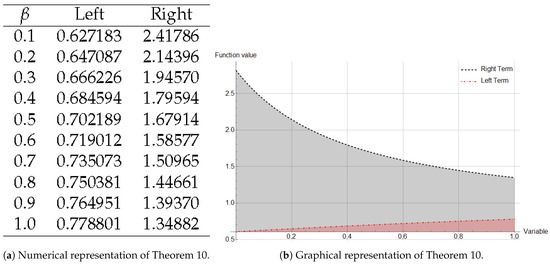
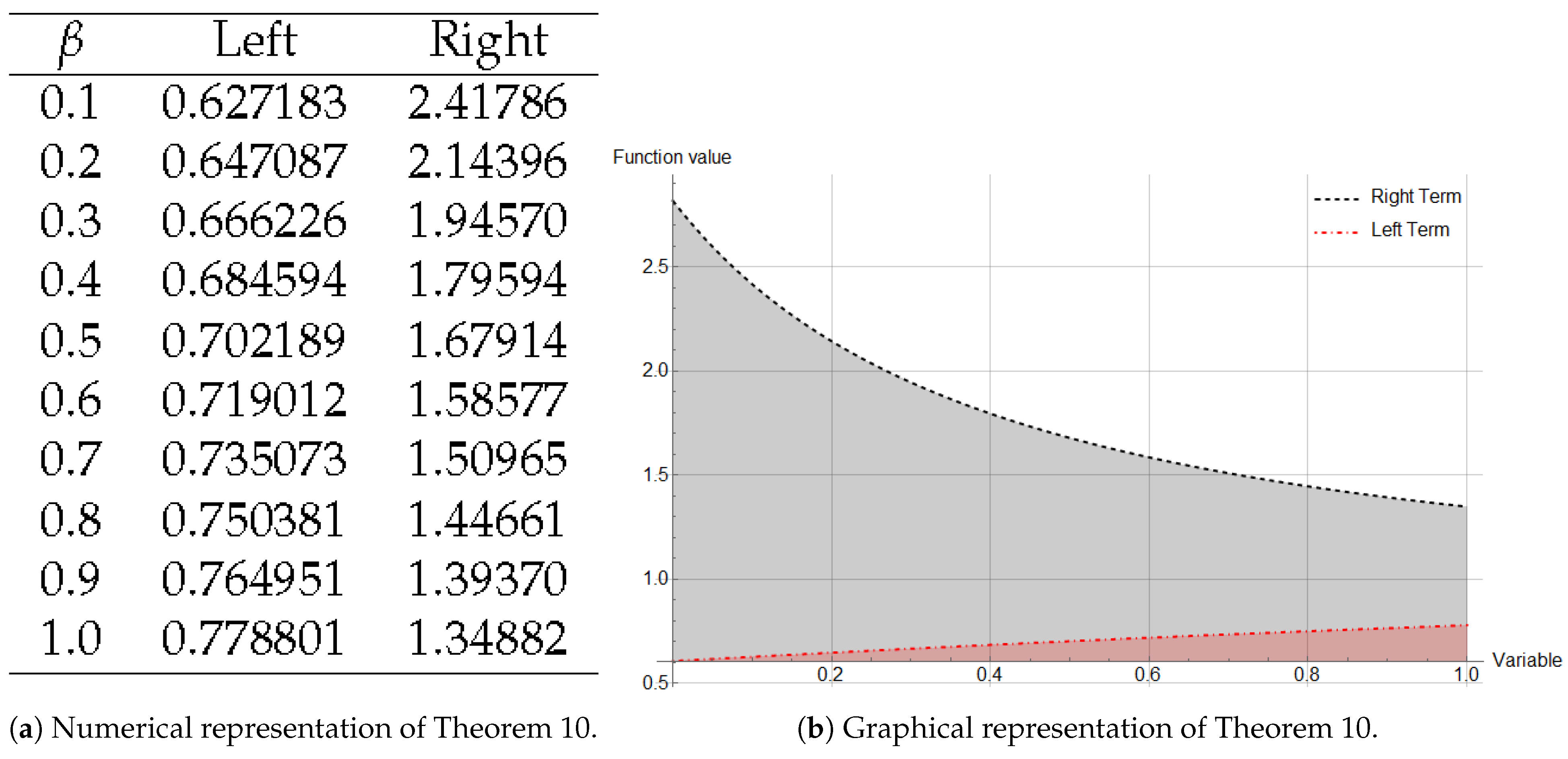
Theorem 10.

Let $\mathrm{{\rm Y}}:[0,\infty )\to (0,\infty )$ be an increasing and ${}^{\ast }\mathit{differentiable}$ multiplicatively superquadratic function. If ${\mathrm{{\rm Y}}}^{\ast }$ is ${}^{\ast }\mathit{integrable}$ and $|ln{\mathrm{{\rm Y}}}^{\ast }{|}^{\mathrm{p}}$ is a superquadratic function, then

$$\begin{array}{ll}& \left|{\displaystyle \frac{{\left({\int }_{\vartheta }^{\frac{\vartheta +\upsilon }{2}}{\left({\left(\mathrm{{\rm Y}}\left(\frac{\vartheta +\upsilon }{2}-\varkappa \right)\right)}^{{(\varkappa -\vartheta )}^{\beta -1}}\right)}^{d\varkappa }{\int }_{\frac{\vartheta +\upsilon }{2}}^{\upsilon }{\left({\left(\mathrm{{\rm Y}}\left(\varkappa -\frac{\vartheta +\upsilon }{2}\right)\right)}^{{(\upsilon -\varkappa )}^{\beta -1}}\right)}^{d\varkappa }\right)}^{\frac{\beta }{{(\upsilon -\vartheta )}^{\beta }}}}{{\left(\frac{\mathrm{{\rm Y}}\left(\frac{\vartheta +\upsilon }{2}\right)}{\mathrm{{\rm Y}}\left(0\right)}\right)}^{-2^{(1-\beta )}}{\left({}_{\ast }I_{\frac{\vartheta +\upsilon }{2}}^{\beta }\mathrm{{\rm Y}}\left(\vartheta \right)·{}_{\frac{\vartheta +\upsilon }{2}}I_{\ast }^{\beta }\mathrm{{\rm Y}}\left(\upsilon \right)\right)}^{\frac{\mathsf{\Gamma }(1+\beta )}{{(\upsilon -\vartheta )}^{\beta }}}}}\right|\\ & \le {\left[{\left({\mathrm{{\rm Y}}}^{\ast }\left(\upsilon \right){\mathrm{{\rm Y}}}^{\ast }\left(\vartheta \right)\right)}^{{\displaystyle \frac{(1+3^{\frac{1}{\mathrm{p}}})}{2^{(1+\beta +\frac{2}{\mathrm{p}})}}}}{\left({\mathrm{{\rm Y}}}^{\ast }\left(0\right){\mathrm{{\rm Y}}}^{\ast }\left({\displaystyle \frac{\upsilon -\vartheta }{2}}\right)\right)}^{{\displaystyle \frac{1}{2^{\beta +\frac{1}{\mathrm{p}}}}}}\right]}^{{\displaystyle \frac{\left(\upsilon -\vartheta \right)}{{(\beta \mathrm{q}+1)}^{\frac{1}{\mathrm{q}}}}}},\end{array}$$

(42)

holds for all $\vartheta ,\upsilon \in [0,\infty )$ with $0\le \vartheta <\upsilon$. Where $\mathrm{q}>1$, ${\displaystyle \frac{1}{\mathrm{q}}}+{\displaystyle \frac{1}{\mathrm{p}}}=1.$

Proof. 

Applying Lemma 6 and then taking absolute values on both sides of (36) yields

$$\begin{array}{ll}& \left|{\displaystyle \frac{{\left({\int }_{\vartheta }^{\frac{\vartheta +\upsilon }{2}}{\left({\left(\mathrm{{\rm Y}}\left(\frac{\vartheta +\upsilon }{2}-\varkappa \right)\right)}^{{(\varkappa -\vartheta )}^{\beta -1}}\right)}^{d\varkappa }{\int }_{\frac{\vartheta +\upsilon }{2}}^{\upsilon }{\left({\left(\mathrm{{\rm Y}}\left(\varkappa -\frac{\vartheta +\upsilon }{2}\right)\right)}^{{(\upsilon -\varkappa )}^{\beta -1}}\right)}^{d\varkappa }\right)}^{\frac{\beta }{{(\upsilon -\vartheta )}^{\beta }}}}{{\left(\frac{\mathrm{{\rm Y}}\left(\frac{\vartheta +\upsilon }{2}\right)}{\mathrm{{\rm Y}}\left(0\right)}\right)}^{-2^{(1-\beta )}}{\left({}_{\ast }I_{\frac{\vartheta +\upsilon }{2}}^{\beta }\mathrm{{\rm Y}}\left(\vartheta \right)·{}_{\frac{\vartheta +\upsilon }{2}}I_{\ast }^{\beta }\mathrm{{\rm Y}}\left(\upsilon \right)\right)}^{\frac{\mathsf{\Gamma }(1+\beta )}{{(\upsilon -\vartheta )}^{\beta }}}}}\right|\\ & \le exp\left\{\left(\upsilon -\vartheta \right)\left({\int }_0^{{\displaystyle \frac{1}{2}}}{\gamma }^{\beta }\left(\left|ln\left({\mathrm{{\rm Y}}}^{\ast }\left(\upsilon \gamma +(1-\gamma )\vartheta \right){\mathrm{{\rm Y}}}^{\ast }\left({\displaystyle \frac{\vartheta +\upsilon }{2}}-(\upsilon \gamma +(1-\gamma )\vartheta )\right)\right)\right|\right)d\gamma \right)\right\}\\ & \times exp\left\{\left(\upsilon -\vartheta \right)\left({\int }_{{\displaystyle \frac{1}{2}}}^1{(1-\gamma )}^{\beta }\left(\left|ln\left({\mathrm{{\rm Y}}}^{\ast }\left(\upsilon \gamma +(1-\gamma )\vartheta \right){\mathrm{{\rm Y}}}^{\ast }\left((\upsilon \gamma +(1-\gamma )\vartheta )-{\displaystyle \frac{\vartheta +\upsilon }{2}}\right)\right)\right|\right)d\gamma \right)\right\}.\end{array}$$

Using Hölder inequality, we obtain

$$\begin{array}{ll}& \left|{\displaystyle \frac{{\left({\int }_{\vartheta }^{\frac{\vartheta +\upsilon }{2}}{\left({\left(\mathrm{{\rm Y}}\left(\frac{\vartheta +\upsilon }{2}-\varkappa \right)\right)}^{{(\varkappa -\vartheta )}^{\beta -1}}\right)}^{d\varkappa }{\int }_{\frac{\vartheta +\upsilon }{2}}^{\upsilon }{\left({\left(\mathrm{{\rm Y}}\left(\varkappa -\frac{\vartheta +\upsilon }{2}\right)\right)}^{{(\upsilon -\varkappa )}^{\beta -1}}\right)}^{d\varkappa }\right)}^{\frac{\beta }{{(\upsilon -\vartheta )}^{\beta }}}}{{\left(\frac{\mathrm{{\rm Y}}\left(\frac{\vartheta +\upsilon }{2}\right)}{\mathrm{{\rm Y}}\left(0\right)}\right)}^{-2^{(1-\beta )}}{\left({}_{\ast }I_{\frac{\vartheta +\upsilon }{2}}^{\beta }\mathrm{{\rm Y}}\left(\vartheta \right)·{}_{\frac{\vartheta +\upsilon }{2}}I_{\ast }^{\beta }\mathrm{{\rm Y}}\left(\upsilon \right)\right)}^{\frac{\mathsf{\Gamma }(1+\beta )}{{(\upsilon -\vartheta )}^{\beta }}}}}\right|\\ & \le exp\left\{\left(\upsilon -\vartheta \right){\left({\int }_0^{{\displaystyle \frac{1}{2}}}{\gamma }^{\mathrm{q}\beta }d\gamma \right)}^{{\displaystyle \frac{1}{\mathrm{q}}}}{\left({\int }_0^{{\displaystyle \frac{1}{2}}}\left({\left|ln\left({\mathrm{{\rm Y}}}^{\ast }\left(\upsilon \gamma +(1-\gamma )\vartheta \right)\right)\right|}^{\mathrm{p}}\right)d\gamma \right)}^{{\displaystyle \frac{1}{\mathrm{p}}}}\right\}\\ & \times exp\left\{\left(\upsilon -\vartheta \right){\left({\int }_0^{{\displaystyle \frac{1}{2}}}{\gamma }^{\mathrm{q}\beta }d\gamma \right)}^{{\displaystyle \frac{1}{\mathrm{q}}}}{\left({\int }_0^{{\displaystyle \frac{1}{2}}}\left({\left|ln\left({\mathrm{{\rm Y}}}^{\ast }\left({\displaystyle \frac{\vartheta +\upsilon }{2}}-(\upsilon \gamma +(1-\gamma )\vartheta )\right)\right)\right|}^{\mathrm{p}}\right)d\gamma \right)}^{{\displaystyle \frac{1}{\mathrm{p}}}}\right\}\\ & \times exp\left\{\left(\upsilon -\vartheta \right){\left({\int }_{{\displaystyle \frac{1}{2}}}^1{(1-\gamma )}^{\mathrm{q}\beta }d\gamma \right)}^{{\displaystyle \frac{1}{\mathrm{q}}}}{\left({\int }_{{\displaystyle \frac{1}{2}}}^1\left({\left|ln\left({\mathrm{{\rm Y}}}^{\ast }\left(\upsilon \gamma +(1-\gamma )\vartheta \right)\right)\right|}^{\mathrm{p}}\right)d\gamma \right)}^{{\displaystyle \frac{1}{\mathrm{p}}}}\right\}\\ & \times exp\left\{\left(\upsilon -\vartheta \right){\left({\int }_{{\displaystyle \frac{1}{2}}}^1{(1-\gamma )}^{\mathrm{q}\beta }d\gamma \right)}^{{\displaystyle \frac{1}{\mathrm{q}}}}{\left({\int }_{{\displaystyle \frac{1}{2}}}^1\left({\left|ln\left({\mathrm{{\rm Y}}}^{\ast }\left(\upsilon \gamma +(1-\gamma )\vartheta -{\displaystyle \frac{\vartheta +\upsilon }{2}}\right)\right)\right|}^{\mathrm{p}}\right)d\gamma \right)}^{{\displaystyle \frac{1}{\mathrm{p}}}}\right\}.\end{array}$$

Since $|ln\left({\mathrm{{\rm Y}}}^{\ast }\right){|}^{\mathrm{p}}$ is a superquadratic. Moreover, noting that $|ln{\mathrm{{\rm Y}}}^{\ast }{|}^{\mathrm{p}}\ge 0$, Lemma 2 ensures that $|ln{\mathrm{{\rm Y}}}^{\ast }{|}^{\mathrm{p}}$ is a convex function. Therefore, by invoking the definition of convexity together with the classical Hermite–Hadamard-type inequality for convex functions, we obtain

$$\begin{array}{ll}& \left|{\displaystyle \frac{{\left({\int }_{\vartheta }^{\frac{\vartheta +\upsilon }{2}}{\left({\left(\mathrm{{\rm Y}}\left(\frac{\vartheta +\upsilon }{2}-\varkappa \right)\right)}^{{(\varkappa -\vartheta )}^{\beta -1}}\right)}^{d\varkappa }{\int }_{\frac{\vartheta +\upsilon }{2}}^{\upsilon }{\left({\left(\mathrm{{\rm Y}}\left(\varkappa -\frac{\vartheta +\upsilon }{2}\right)\right)}^{{(\upsilon -\varkappa )}^{\beta -1}}\right)}^{d\varkappa }\right)}^{\frac{\beta }{{(\upsilon -\vartheta )}^{\beta }}}}{{\left(\frac{\mathrm{{\rm Y}}\left(\frac{\vartheta +\upsilon }{2}\right)}{\mathrm{{\rm Y}}\left(0\right)}\right)}^{-2^{(1-\beta )}}{\left({}_{\ast }I_{\frac{\vartheta +\upsilon }{2}}^{\beta }\mathrm{{\rm Y}}\left(\vartheta \right)·{}_{\frac{\vartheta +\upsilon }{2}}I_{\ast }^{\beta }\mathrm{{\rm Y}}\left(\upsilon \right)\right)}^{\frac{\mathsf{\Gamma }(1+\beta )}{{(\upsilon -\vartheta )}^{\beta }}}}}\right|\\ & \le exp\left\{{\displaystyle \frac{\left(\upsilon -\vartheta \right)}{2^{\frac{1+\beta \mathrm{q}}{\mathrm{q}}}{(\beta \mathrm{q}+1)}^{\frac{1}{\mathrm{q}}}}}{\left({\int }_0^{{\displaystyle \frac{1}{2}}}\left(\gamma {\left|ln\left({\mathrm{{\rm Y}}}^{\ast }\left(\upsilon \right)\right)\right|}^{\mathrm{p}}+(1-\gamma ){\left|ln\left({\mathrm{{\rm Y}}}^{\ast }\left(\vartheta \right)\right)\right|}^{\mathrm{p}}\right)d\gamma \right)}^{{\displaystyle \frac{1}{\mathrm{p}}}}\right\}\\ & \times exp\left\{{\displaystyle \frac{\left(\upsilon -\vartheta \right)}{2^{\frac{1+\beta \mathrm{q}}{\mathrm{q}}}{(\beta \mathrm{q}+1)}^{\frac{1}{\mathrm{q}}}}}{\left({\displaystyle \frac{{\left|ln\left({\mathrm{{\rm Y}}}^{\ast }\left(0\right)\right)\right|}^{\mathrm{p}}+{\left|ln\left({\mathrm{{\rm Y}}}^{\ast }\left(\frac{\upsilon -\vartheta }{2}\right)\right)\right|}^{\mathrm{p}}}{4}}\right)}^{{\displaystyle \frac{1}{\mathrm{p}}}}\right\}\\ & \times exp\left\{{\displaystyle \frac{\left(\upsilon -\vartheta \right)}{2^{\frac{1+\beta \mathrm{q}}{\mathrm{q}}}{(\beta \mathrm{q}+1)}^{\frac{1}{\mathrm{q}}}}}{\left({\int }_{{\displaystyle \frac{1}{2}}}^1\left(\gamma {\left|ln\left({\mathrm{{\rm Y}}}^{\ast }\left(\upsilon \right)\right)\right|}^{\mathrm{p}}+(1-\gamma ){\left|ln\left({\mathrm{{\rm Y}}}^{\ast }\left(\vartheta \right)\right)\right|}^{\mathrm{p}}\right)d\gamma \right)}^{{\displaystyle \frac{1}{\mathrm{p}}}}\right\}\\ & \times exp\left\{{\displaystyle \frac{\left(\upsilon -\vartheta \right)}{2^{\frac{1+\beta \mathrm{q}}{\mathrm{q}}}{(\beta \mathrm{q}+1)}^{\frac{1}{\mathrm{q}}}}}{\left({\displaystyle \frac{{\left|ln\left({\mathrm{{\rm Y}}}^{\ast }\left(0\right)\right)\right|}^{\mathrm{p}}+{\left|ln\left({\mathrm{{\rm Y}}}^{\ast }\left(\frac{\upsilon -\vartheta }{2}\right)\right)\right|}^{\mathrm{p}}}{4}}\right)}^{{\displaystyle \frac{1}{\mathrm{p}}}}\right\}\\ & =exp\left\{{\displaystyle \frac{\left(\upsilon -\vartheta \right)}{2^{\frac{1+\beta \mathrm{q}}{\mathrm{q}}}{(\beta \mathrm{q}+1)}^{\frac{1}{\mathrm{q}}}}}{\left({\displaystyle \frac{{\left|ln\left({\mathrm{{\rm Y}}}^{\ast }\left(\upsilon \right)\right)\right|}^{\mathrm{p}}+3{\left|ln\left({\mathrm{{\rm Y}}}^{\ast }\left(\vartheta \right)\right)\right|}^{\mathrm{p}}}{8}}\right)}^{{\displaystyle \frac{1}{\mathrm{p}}}}\right\}\\ & \times exp\left\{{\displaystyle \frac{2\left(\upsilon -\vartheta \right)}{2^{\frac{1+\beta \mathrm{q}}{\mathrm{q}}}{(\beta \mathrm{q}+1)}^{\frac{1}{\mathrm{q}}}}}{\left({\displaystyle \frac{{\left|ln\left({\mathrm{{\rm Y}}}^{\ast }\left(0\right)\right)\right|}^{\mathrm{p}}+{\left|ln\left({\mathrm{{\rm Y}}}^{\ast }\left(\frac{\upsilon -\vartheta }{2}\right)\right)\right|}^{\mathrm{p}}}{4}}\right)}^{{\displaystyle \frac{1}{\mathrm{p}}}}\right\}\\ & \times exp\left\{{\displaystyle \frac{\left(\upsilon -\vartheta \right)}{2^{\frac{1+\beta \mathrm{q}}{\mathrm{q}}}{(\beta \mathrm{q}+1)}^{\frac{1}{\mathrm{q}}}}}{\left({\displaystyle \frac{3{\left|ln\left({\mathrm{{\rm Y}}}^{\ast }\left(\upsilon \right)\right)\right|}^{\mathrm{p}}+{\left|ln\left({\mathrm{{\rm Y}}}^{\ast }\left(\vartheta \right)\right)\right|}^{\mathrm{p}}}{8}}\right)}^{{\displaystyle \frac{1}{\mathrm{p}}}}\right\}.\end{array}$$

This further implies that

$$\begin{array}{ll}& \left|\mathrm{{\rm Y}}\left({\displaystyle \frac{\vartheta +\upsilon }{2}}\right){\left({\int }_{\vartheta }^{\upsilon }{\left({\displaystyle \frac{\mathrm{{\rm Y}}\left(\left|\varkappa -\frac{\vartheta +\upsilon }{2}\right|\right)}{\mathrm{{\rm Y}}\left(\varkappa \right)}}\right)}^{d\varkappa }\right)}^{{\displaystyle \frac{1}{\upsilon -\vartheta }}}\right|{\displaystyle \frac{1}{\mathrm{{\rm Y}}\left(0\right)}}\\ & \le exp\left\{{\displaystyle \frac{\left(\upsilon -\vartheta \right)}{2^{(1+\beta +\frac{2}{\mathrm{p}})}{(\beta \mathrm{q}+1)}^{\frac{1}{\mathrm{q}}}}}\right[{\left({\left|ln\left({\mathrm{{\rm Y}}}^{\ast }\left(\upsilon \right)\right)\right|}^{\mathrm{p}}+3{\left|ln\left({\mathrm{{\rm Y}}}^{\ast }\left(\vartheta \right)\right)\right|}^{\mathrm{p}}\right)}^{{\displaystyle \frac{1}{\mathrm{p}}}}\\ & +{\left(3{\left|ln\left({\mathrm{{\rm Y}}}^{\ast }\left(\upsilon \right)\right)\right|}^{\mathrm{p}}+{\left|ln\left({\mathrm{{\rm Y}}}^{\ast }\left(\vartheta \right)\right)\right|}^{\mathrm{p}}\right)}^{{\displaystyle \frac{1}{\mathrm{p}}}}\left]\right\}\\ & \times exp\left\{{\displaystyle \frac{\left(\upsilon -\vartheta \right)}{2^{\beta +\frac{1}{\mathrm{p}}}{(\beta \mathrm{q}+1)}^{\frac{1}{\mathrm{q}}}}}{\left({\left|ln\left({\mathrm{{\rm Y}}}^{\ast }\left(0\right)\right)\right|}^{\mathrm{p}}+{\left|ln\left({\mathrm{{\rm Y}}}^{\ast }\left({\displaystyle \frac{\upsilon -\vartheta }{2}}\right)\right)\right|}^{\mathrm{p}}\right)}^{{\displaystyle \frac{1}{\mathrm{p}}}}\right\}.\end{array}$$

(43)

Since $ln{\mathrm{{\rm Y}}}^{\ast }\left(\varkappa \right)\ge 0$, it follows that $|ln{\mathrm{{\rm Y}}}^{\ast }\left(\varkappa \right)|=ln\left({\mathrm{{\rm Y}}}^{\ast }\left(\varkappa \right)\right)$. Using this observation, we can further simplify (43) by applying the inequality ${(\vartheta +\upsilon )}^{\mathrm{s}}\le {\vartheta }^{\mathrm{s}}+{\upsilon }^{\mathrm{s}},\forall \mathrm{s}\in [0,1).$

$$\begin{array}{ll}& \left|{\displaystyle \frac{{\left({\int }_{\vartheta }^{\frac{\vartheta +\upsilon }{2}}{\left({\left(\mathrm{{\rm Y}}\left(\frac{\vartheta +\upsilon }{2}-\varkappa \right)\right)}^{{(\varkappa -\vartheta )}^{\beta -1}}\right)}^{d\varkappa }{\int }_{\frac{\vartheta +\upsilon }{2}}^{\upsilon }{\left({\left(\mathrm{{\rm Y}}\left(\varkappa -\frac{\vartheta +\upsilon }{2}\right)\right)}^{{(\upsilon -\varkappa )}^{\beta -1}}\right)}^{d\varkappa }\right)}^{\frac{\beta }{{(\upsilon -\vartheta )}^{\beta }}}}{{\left(\frac{\mathrm{{\rm Y}}\left(\frac{\vartheta +\upsilon }{2}\right)}{\mathrm{{\rm Y}}\left(0\right)}\right)}^{-2^{(1-\beta )}}{\left({}_{\ast }I_{\frac{\vartheta +\upsilon }{2}}^{\beta }\mathrm{{\rm Y}}\left(\vartheta \right)·{}_{\frac{\vartheta +\upsilon }{2}}I_{\ast }^{\beta }\mathrm{{\rm Y}}\left(\upsilon \right)\right)}^{\frac{\mathsf{\Gamma }(1+\beta )}{{(\upsilon -\vartheta )}^{\beta }}}}}\right|\\ & \le exp\left\{{\displaystyle \frac{\left(\upsilon -\vartheta \right)}{2^{(1+\beta +\frac{2}{\mathrm{p}})}{(\beta \mathrm{q}+1)}^{\frac{1}{\mathrm{q}}}}}\left[ln\left({\mathrm{{\rm Y}}}^{\ast }\left(\upsilon \right)\right)+3^{{\displaystyle \frac{1}{\mathrm{p}}}}ln\left({\mathrm{{\rm Y}}}^{\ast }\left(\vartheta \right)\right)+3^{{\displaystyle \frac{1}{\mathrm{p}}}}ln\left({\mathrm{{\rm Y}}}^{\ast }\left(\upsilon \right)\right)+ln\left({\mathrm{{\rm Y}}}^{\ast }\left(\vartheta \right)\right)\right]\right\}\\ & \times exp\left\{{\displaystyle \frac{\left(\upsilon -\vartheta \right)}{2^{\beta +\frac{1}{\mathrm{p}}}{(\beta \mathrm{q}+1)}^{\frac{1}{\mathrm{q}}}}}\left(ln\left({\mathrm{{\rm Y}}}^{\ast }\left(0\right)\right)+ln\left({\mathrm{{\rm Y}}}^{\ast }\left({\displaystyle \frac{\upsilon -\vartheta }{2}}\right)\right)\right)\right\}\\ & =exp\left\{{\displaystyle \frac{(1+3^{\frac{1}{\mathrm{p}}})\left(\upsilon -\vartheta \right)}{2^{(1+\beta +\frac{2}{\mathrm{p}})}{(\beta \mathrm{q}+1)}^{\frac{1}{\mathrm{q}}}}}\left[ln\left({\mathrm{{\rm Y}}}^{\ast }\left(\upsilon \right){\mathrm{{\rm Y}}}^{\ast }\left(\vartheta \right)\right)\right]\right\}\\ & \times exp\left\{{\displaystyle \frac{\left(\upsilon -\vartheta \right)}{2^{\beta +\frac{1}{\mathrm{p}}}{(\beta \mathrm{q}+1)}^{\frac{1}{\mathrm{q}}}}}\left[ln\left({\mathrm{{\rm Y}}}^{\ast }\left(0\right){\mathrm{{\rm Y}}}^{\ast }\left({\displaystyle \frac{\upsilon -\vartheta }{2}}\right)\right)\right]\right\}\\ & =exp\left\{ln{\left[{\left({\mathrm{{\rm Y}}}^{\ast }\left(\upsilon \right){\mathrm{{\rm Y}}}^{\ast }\left(\vartheta \right)\right)}^{{\displaystyle \frac{(1+3^{\frac{1}{\mathrm{p}}})}{2^{(1+\beta +\frac{2}{\mathrm{p}})}}}}{\left({\mathrm{{\rm Y}}}^{\ast }\left(0\right){\mathrm{{\rm Y}}}^{\ast }\left({\displaystyle \frac{\upsilon -\vartheta }{2}}\right)\right)}^{{\displaystyle \frac{1}{2^{\beta +\frac{1}{\mathrm{p}}}}}}\right]}^{{\displaystyle \frac{\left(\upsilon -\vartheta \right)}{{(\beta \mathrm{q}+1)}^{\frac{1}{\mathrm{q}}}}}}\right\}\\ & ={\left[{\left({\mathrm{{\rm Y}}}^{\ast }\left(\upsilon \right){\mathrm{{\rm Y}}}^{\ast }\left(\vartheta \right)\right)}^{{\displaystyle \frac{(1+3^{\frac{1}{\mathrm{p}}})}{2^{(1+\beta +\frac{2}{\mathrm{p}})}}}}{\left({\mathrm{{\rm Y}}}^{\ast }\left(0\right){\mathrm{{\rm Y}}}^{\ast }\left({\displaystyle \frac{\upsilon -\vartheta }{2}}\right)\right)}^{{\displaystyle \frac{1}{2^{\beta +\frac{1}{\mathrm{p}}}}}}\right]}^{{\displaystyle \frac{\left(\upsilon -\vartheta \right)}{{(\beta \mathrm{q}+1)}^{\frac{1}{\mathrm{q}}}}}}.\end{array}$$

This completes the proof. □

Remark 5.

As a special case of Theorem 10, choosing $\beta =1$ leads to Theorem 6.

We conclude this section with an example that demonstrates the accuracy and reliability of Theorems 9 and 10 through numerical computations and graphical illustrations.

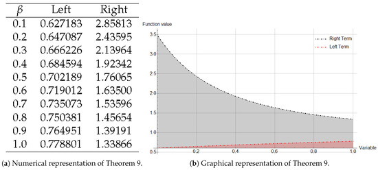
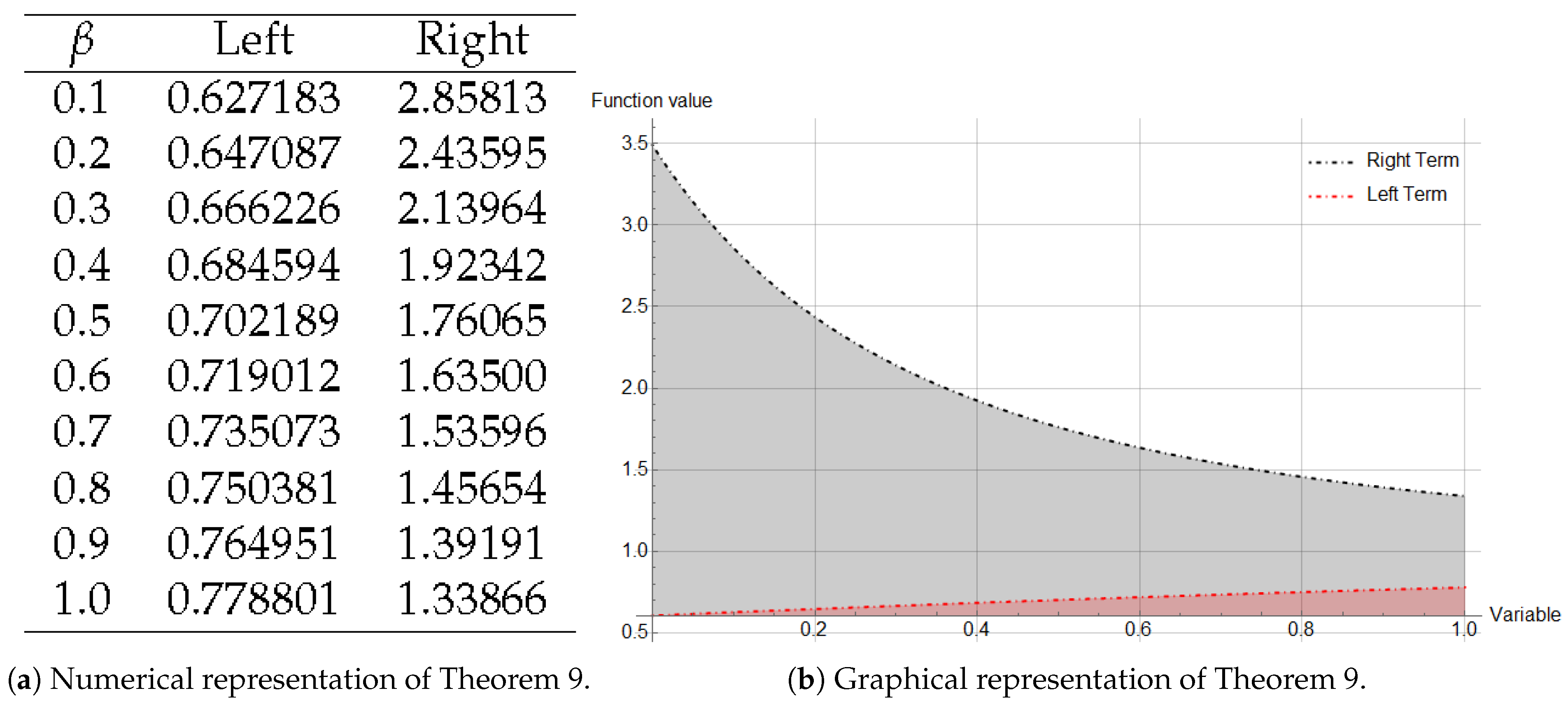
Example 3.

We consider the function $\mathrm{{\rm Y}}\left(\varkappa \right)=exp\left\{{\varkappa }^2\right\}$, which is multiplicatively superquadratic on $[0,\infty )$. For different selections of the parameters involved in Theorems 9 and 10, we obtain representative numerical computations and corresponding graphical depictions that illustrate the applicability of our results. In particular, upon setting $\vartheta =0$ and $\upsilon =1$ in Theorem 9, we compute the respective left-, middle-, and right-hand sides of the inequality.

$$\begin{array}{ll}& \mathit{Left}\mathit{Term}=exp\{{\displaystyle \frac{{0.5}^{1+\beta }}{\left(\beta +1\right)(2+\beta )}}+{\displaystyle \frac{0.5\beta exp\left\{-0.693147\beta \right\}}{{\beta }^3+3{\beta }^2+2\beta }}\\ & -{\displaystyle \frac{{0.25}^{\beta }\left({0.5}^{\beta }\right)}{2+\beta }}-\beta \left({\displaystyle \frac{2\mathsf{\Gamma }\left(\beta \right)}{\mathsf{\Gamma }(3+\beta )}}-{\displaystyle \frac{1}{24}}{}_{2}F_1\left(3,1-\beta ;4;\frac{1}{2}\right)\right)\}\\ & \mathit{Right}\mathit{Term}=exp\left\{{\displaystyle \frac{5+2\beta }{2^{\beta +1}(2+\beta )(1+\beta )}}\right\}\end{array}$$

These computations lead to the numerical results listed in Figure 2a and the graphical representation in Figure 2b.

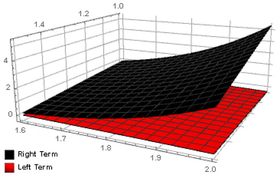
Analogously, taking $\vartheta =0$, $\upsilon =1$, $\mathrm{p}=2$, and $\mathrm{q}=2$ in Theorem 10, we compute the associated left-, middle-, and right-hand expressions of the inequality.

$$\begin{array}{ll}& \mathit{Left}\mathit{Term}=exp\{{\displaystyle \frac{{0.5}^{1+\beta }}{\left(\beta +1\right)(2+\beta )}}+{\displaystyle \frac{0.5\beta exp\left\{-0.693147\beta \right\}}{{\beta }^3+3{\beta }^2+2\beta }}\\ & -{\displaystyle \frac{{0.25}^{\beta }\left({0.5}^{\beta }\right)}{2+\beta }}-\beta \left({\displaystyle \frac{2\mathsf{\Gamma }\left(\beta \right)}{\mathsf{\Gamma }(3+\beta )}}-{\displaystyle \frac{1}{24}}{}_{2}F_1\left(3,1-\beta ;4;\frac{1}{2}\right)\right)\}\\ & \mathit{Right}\mathit{Term}=exp\left\{\left({\displaystyle \frac{1+\sqrt{3}}{2^{\beta +2}}}+{\displaystyle \frac{1}{2^{\beta +\frac{3}{2}}}}\right){\displaystyle \frac{1}{\sqrt{2\beta +1}}}\right\}.\end{array}$$

These computations lead to the numerical results listed in Figure 3a and the graphical representation in Figure 3.

The graphical illustrations verify the validity of the inequalities by showing that the curve corresponding to the right-hand side consistently lies above the curve corresponding to the left-hand side throughout the considered domain. Likewise, the tabulated numerical results demonstrate that the computed values of the left-hand side remain smaller than (or equal to, where applicable) the corresponding values of the right-hand side for all selected parameter values.

6. Fractional Trapezoid-Type Inequalities for Multiplicatively Superquadratic Functions

This section deals with the derivation of a novel identity for ${}^{\ast }\mathrm{integrable}$ multiplicatively superquadratic functions in the context of multiplicative calculus by utilizing multiplicative Riemann–Liouville fractional integrals. Using this identity in conjunction with Petrovič’s inequality, we then establish novel fractional trapezoid-type inequalities for this class of functions.

Lemma 7.

Let $\mathrm{{\rm Y}}:[0,\infty )\to (0,\infty )$ be an increasing and ${}^{\ast }\mathit{differentiable}$ function. If ${\mathrm{{\rm Y}}}^{\ast }$ is ${}^{\ast }\mathit{integrable}$, then

$$\begin{array}{ll}& {\left({\int }_0^1{\left({\displaystyle \frac{{\left({\mathrm{{\rm Y}}}^{\ast }\left(\upsilon \gamma +(1-\gamma )\vartheta \right)\right)}^{{(1-\gamma )}^{\beta }}{\left({\mathrm{{\rm Y}}}^{\ast }\left((\upsilon -\vartheta )\gamma \right)\right)}^{{(1-\gamma )}^{2\beta }}{\left({\mathrm{{\rm Y}}}^{\ast }\left((\upsilon -\vartheta )(1-\gamma )\right)\right)}^{{\gamma }^{2\beta }}}{{\left({\mathrm{{\rm Y}}}^{\ast }\left(\upsilon \gamma +(1-\gamma )\vartheta \right)\right)}^{{\gamma }^{\beta }}}}\right)}^{d\gamma }\right)}^{{\displaystyle \frac{\upsilon -\vartheta }{2}}}\\ & ={\displaystyle \frac{{\left[{}_{\vartheta }\mathrm{I}_{\ast }^{\beta }\mathrm{{\rm Y}}\left(\upsilon \right)·{}_{\ast }\mathrm{I}_{\upsilon }^{\beta }\mathrm{{\rm Y}}\left(\vartheta \right)\right]}^{\frac{\mathsf{\Gamma }(1+\beta )}{2{(\upsilon -\vartheta )}^{\beta }}}{\left({\left({\int }_{\vartheta }^{\upsilon }\left({\left(\mathrm{{\rm Y}}(\varkappa -\vartheta )\right)}^{{(\upsilon -\varkappa )}^{2\beta -1}}{\left(\mathrm{{\rm Y}}(\upsilon -\varkappa )\right)}^{{(\varkappa -\vartheta )}^{2\beta -1}}\right)\right)}^{d\varkappa }\right)}^{\frac{\beta }{{(\upsilon -\vartheta )}^{2\beta }}}}{\sqrt{\mathrm{{\rm Y}}\left(\vartheta \right)\mathrm{{\rm Y}}\left(\upsilon \right)}\left(\mathrm{{\rm Y}}\left(0\right)\right)}},\end{array}$$

(44)

holds for all $\vartheta ,\upsilon \in [0,\infty )$ with $0\le \vartheta <\upsilon$ and $\beta >0$.

Proof. 

The following identity follows directly from the properties established in Proposition 1, together with the ${}^{\ast }\mathrm{integration}$ by parts formula presented in Theorem 3.

$$\begin{array}{ll}& \mathrm{I}={\left({\int }_0^1{\left({\displaystyle \frac{{\left({\mathrm{{\rm Y}}}^{\ast }\left(\upsilon \gamma +(1-\gamma )\vartheta \right)\right)}^{{(1-\gamma )}^{\beta }}{\left({\mathrm{{\rm Y}}}^{\ast }\left((\upsilon -\vartheta )\gamma \right)\right)}^{{(1-\gamma )}^{2\beta }}{\left({\mathrm{{\rm Y}}}^{\ast }\left((\upsilon -\vartheta )(1-\gamma )\right)\right)}^{{\gamma }^{2\beta }}}{{\left({\mathrm{{\rm Y}}}^{\ast }\left(\upsilon \gamma +(1-\gamma )\vartheta \right)\right)}^{{\gamma }^{\beta }}}}\right)}^{d\gamma }\right)}^{{\displaystyle \frac{\upsilon -\vartheta }{2}}}\\ & ={\left({\int }_0^1{\left({\left({\mathrm{{\rm Y}}}^{\ast }\left(\upsilon \gamma +(1-\gamma )\vartheta \right)\right)}^{{(1-\gamma )}^{\beta }}\right)}^{d\gamma }\right)}^{{\displaystyle \frac{\upsilon -\vartheta }{2}}}{\left({\int }_0^1{\left({\left({\mathrm{{\rm Y}}}^{\ast }\left(\upsilon \gamma +(1-\gamma )\vartheta \right)\right)}^{-{\gamma }^{\beta }}\right)}^{d\gamma }\right)}^{{\displaystyle \frac{\upsilon -\vartheta }{2}}}\\ & \times {\left({\int }_0^1{\left({\left({\mathrm{{\rm Y}}}^{\ast }\left((\upsilon -\vartheta )\gamma \right)\right)}^{{(1-\gamma )}^{2\beta }}\right)}^{d\gamma }\right)}^{{\displaystyle \frac{\upsilon -\vartheta }{2}}}{\left({\int }_0^1{\left({\left({\mathrm{{\rm Y}}}^{\ast }\left((\upsilon -\vartheta )(1-\gamma )\right)\right)}^{{\gamma }^{2\beta }}\right)}^{d\gamma }\right)}^{{\displaystyle \frac{\upsilon -\vartheta }{2}}}\\ & ={\displaystyle \frac{{\int }_0^1{\left({\left(\mathrm{{\rm Y}}\left(\upsilon \gamma +(1-\gamma )\vartheta \right)\right)}^{\frac{\beta {(1-\gamma )}^{\beta -1}}{2}}\right)}^{d\gamma }{\int }_0^1{\left({\left(\mathrm{{\rm Y}}\left(\upsilon \gamma +(1-\gamma )\vartheta \right)\right)}^{\frac{\beta {\gamma }^{\beta -1}}{2}}\right)}^{d\gamma }}{\sqrt{\mathrm{{\rm Y}}\left(\vartheta \right)\mathrm{{\rm Y}}\left(\upsilon \right)}}}\\ & \times {\displaystyle \frac{{\int }_0^1{\left({\left(\mathrm{{\rm Y}}\left((\upsilon -\vartheta )\gamma \right)\right)}^{\beta {(1-\gamma )}^{2\beta -1}}\right)}^{d\gamma }{\int }_0^1{\left({\left(\mathrm{{\rm Y}}\left((\upsilon -\vartheta )(1-\gamma )\right)\right)}^{\beta {\gamma }^{2\beta -1}}\right)}^{d\gamma }}{\mathrm{{\rm Y}}\left(0\right)}}.\end{array}$$

(45)

By performing a change of variables in (45), we obtain

$$\begin{array}{ll}& \mathrm{I}={\displaystyle \frac{{\left({\int }_{\vartheta }^{\upsilon }{\left({\left(\mathrm{{\rm Y}}\left(\varkappa \right)\right)}^{{(\upsilon -\varkappa )}^{\beta -1}}\right)}^{d\varkappa }\right)}^{\frac{\beta }{2{(\upsilon -\vartheta )}^{\beta }}}{\left({\int }_{\vartheta }^{\upsilon }{\left({\left(\mathrm{{\rm Y}}\left(\varkappa \right)\right)}^{{(\varkappa -\vartheta )}^{\beta -1}}\right)}^{d\varkappa }\right)}^{\frac{\beta }{2{(\upsilon -\vartheta )}^{\beta }}}}{\sqrt{\mathrm{{\rm Y}}\left(\vartheta \right)\mathrm{{\rm Y}}\left(\upsilon \right)}}}\\ & \times {\displaystyle \frac{{\left({\int }_{\vartheta }^{\upsilon }{\left({\left(\mathrm{{\rm Y}}(\varkappa -\vartheta )\right)}^{{(\upsilon -\varkappa )}^{2\beta -1}}\right)}^{d\varkappa }\right)}^{\frac{\beta }{{(\upsilon -\vartheta )}^{2\beta }}}{\left({\int }_{\vartheta }^{\upsilon }{\left({\left(\mathrm{{\rm Y}}(\upsilon -\varkappa )\right)}^{{(\varkappa -\vartheta )}^{2\beta -1}}\right)}^{d\varkappa }\right)}^{\frac{\beta }{{(\upsilon -\vartheta )}^{2\beta }}}}{\mathrm{{\rm Y}}\left(0\right)}}\\ & ={\displaystyle \frac{{\left[{}_{\vartheta }\mathrm{I}_{\ast }^{\beta }\mathrm{{\rm Y}}\left(\upsilon \right)·{}_{\ast }\mathrm{I}_{\upsilon }^{\beta }\mathrm{{\rm Y}}\left(\vartheta \right)\right]}^{\frac{\mathsf{\Gamma }(1+\beta )}{2{(\upsilon -\vartheta )}^{\beta }}}}{\sqrt{\mathrm{{\rm Y}}\left(\vartheta \right)\mathrm{{\rm Y}}\left(\upsilon \right)}\left(\mathrm{{\rm Y}}\left(0\right)\right)}}\\ & \times {\left({\left({\int }_{\vartheta }^{\upsilon }\left({\left(\mathrm{{\rm Y}}(\varkappa -\vartheta )\right)}^{{(\upsilon -\varkappa )}^{2\beta -1}}{\left(\mathrm{{\rm Y}}(\upsilon -\varkappa )\right)}^{{(\varkappa -\vartheta )}^{2\beta -1}}\right)\right)}^{d\varkappa }\right)}^{{\displaystyle \frac{\beta }{{(\upsilon -\vartheta )}^{2\beta }}}}.\end{array}$$

This completes the proof. □

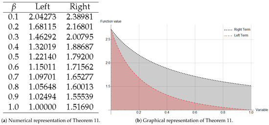
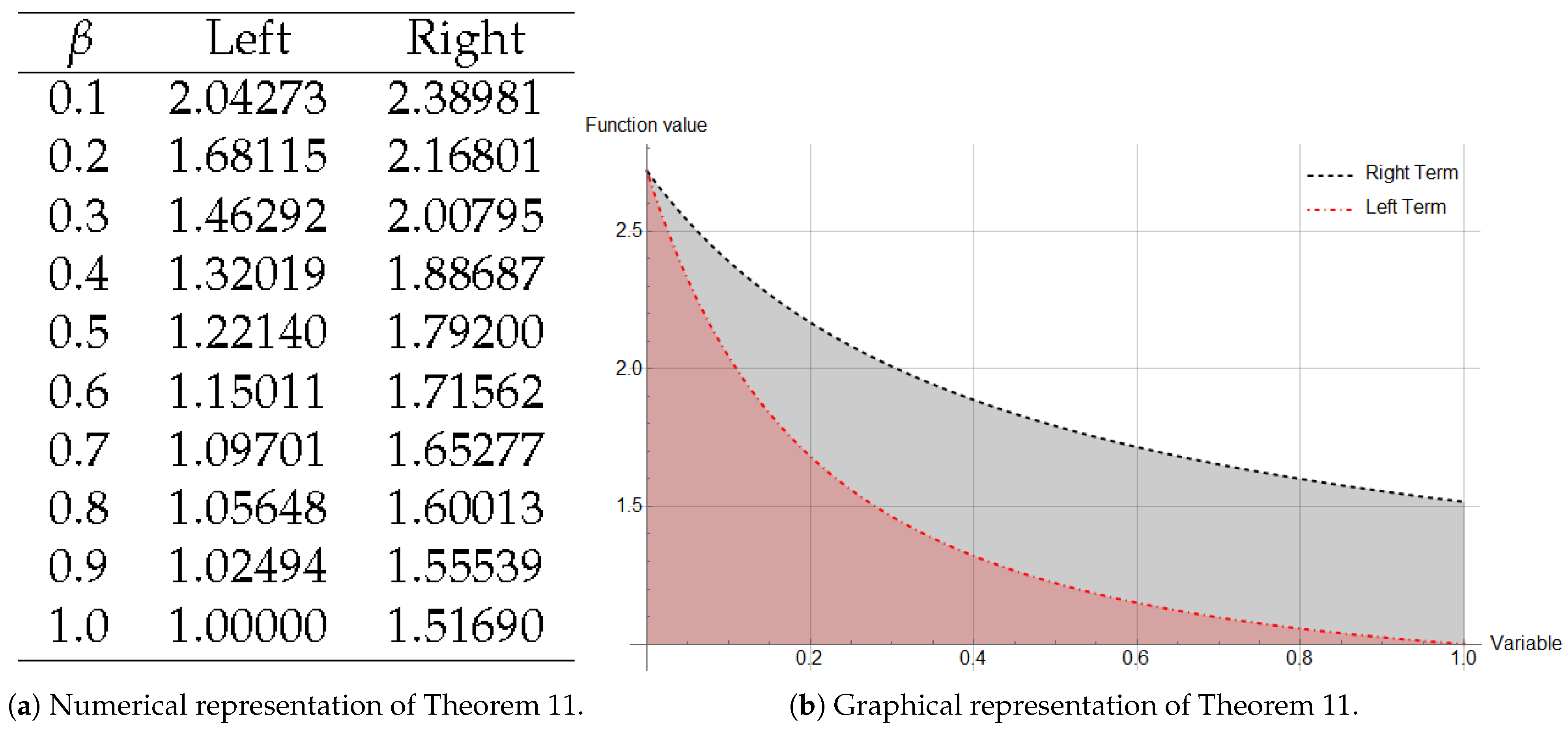
Theorem 11.

Let $\mathrm{{\rm Y}}:[0,\infty )\to (0,\infty )$ be an increasing and ${}^{\ast }\mathit{differentiable}$ multiplicatively superquadratic function. If ${\mathrm{{\rm Y}}}^{\ast }$ is ${}^{\ast }\mathit{integrable}$ and $|{\mathrm{{\rm Y}}}^{\ast }|$ is a multiplicatively superquadratic function, then

$$\begin{array}{l}\left|{\displaystyle \frac{{\left[{}_{\vartheta }\mathrm{I}_{\ast }^{\beta }\mathrm{{\rm Y}}\left(\upsilon \right)·{}_{\ast }\mathrm{I}_{\upsilon }^{\beta }\mathrm{{\rm Y}}\left(\vartheta \right)\right]}^{\frac{\mathsf{\Gamma }(1+\beta )}{2{(\upsilon -\vartheta )}^{\beta }}}{\left({\left({\int }_{\vartheta }^{\upsilon }\left({\left(\mathrm{{\rm Y}}(\varkappa -\vartheta )\right)}^{{(\upsilon -\varkappa )}^{2\beta -1}}{\left(\mathrm{{\rm Y}}(\upsilon -\varkappa )\right)}^{{(\varkappa -\vartheta )}^{2\beta -1}}\right)\right)}^{d\varkappa }\right)}^{\frac{\beta }{{(\upsilon -\vartheta )}^{2\beta }}}}{\sqrt{\mathrm{{\rm Y}}\left(\vartheta \right)\mathrm{{\rm Y}}\left(\upsilon \right)}\left(\mathrm{{\rm Y}}\left(0\right)\right)}}\right|\\ \le {\left({\mathrm{{\rm Y}}}^{\ast }\left(2\upsilon -\vartheta \right){\mathrm{{\rm Y}}}^{\ast }\left(0\right)\right)}^{{\displaystyle \frac{\upsilon -\vartheta }{2(\beta +1)}}}{\left({\mathrm{{\rm Y}}}^{\ast }\left(\upsilon -\vartheta \right){\mathrm{{\rm Y}}}^{\ast }\left(0\right)\right)}^{{\displaystyle \frac{\upsilon -\vartheta }{2(2\beta +1)}}},\end{array}$$

(46)

holds for all $\vartheta ,\upsilon \in [0,\infty )$ with $0\le \vartheta <\upsilon$ and $\beta >0$.

Proof. 

Applying Lemma 7 and then taking absolute values on both sides of (44) yields

$$\begin{array}{ll}& \left|{\displaystyle \frac{{\left[{}_{\vartheta }\mathrm{I}_{\ast }^{\beta }\mathrm{{\rm Y}}\left(\upsilon \right)·{}_{\ast }\mathrm{I}_{\upsilon }^{\beta }\mathrm{{\rm Y}}\left(\vartheta \right)\right]}^{\frac{\mathsf{\Gamma }(1+\beta )}{2{(\upsilon -\vartheta )}^{\beta }}}{\left({\left({\int }_{\vartheta }^{\upsilon }\left({\left(\mathrm{{\rm Y}}(\varkappa -\vartheta )\right)}^{{(\upsilon -\varkappa )}^{2\beta -1}}{\left(\mathrm{{\rm Y}}(\upsilon -\varkappa )\right)}^{{(\varkappa -\vartheta )}^{2\beta -1}}\right)\right)}^{d\varkappa }\right)}^{\frac{\beta }{{(\upsilon -\vartheta )}^{2\beta }}}}{\sqrt{\mathrm{{\rm Y}}\left(\vartheta \right)\mathrm{{\rm Y}}\left(\upsilon \right)}\left(\mathrm{{\rm Y}}\left(0\right)\right)}}\right|\\ & \le exp\left\{{\displaystyle \frac{\upsilon -\vartheta }{2}}\left({\int }_0^1\left|{(1-\gamma )}^{\beta }-{\gamma }^{\beta }\right|\left|ln{\mathrm{{\rm Y}}}^{\ast }\left(\upsilon \gamma +(1-\gamma )\vartheta \right)\right|d\gamma \right)\right\}\\ & \times exp\left\{{\displaystyle \frac{\upsilon -\vartheta }{2}}\left({\int }_0^1{\left(1-\gamma \right)}^{2\beta }\left|ln{\mathrm{{\rm Y}}}^{\ast }\left((\upsilon -\vartheta )\gamma \right)\right|d\gamma \right)\right\}\\ & \times exp\left\{{\displaystyle \frac{\upsilon -\vartheta }{2}}\left({\int }_0^1{\gamma }^{2\beta }\left|ln{\mathrm{{\rm Y}}}^{\ast }\left((\upsilon -\vartheta )(1-\gamma )\right)\right|d\gamma \right)\right\}.\end{array}$$

(47)

Observe that, for all $0<\gamma <1$ and $0<\beta <1$, ${|(1-\gamma )}^{\beta }-{\gamma }^{\beta }|\le |{(1-2\gamma )|}^{\beta }$, and ${\left|(1-\gamma )\right|}^{2\beta }\le |{(1-2\gamma )}^{\beta }+{\gamma }^{2\beta }|.$ Hence, relation (47) takes the simplified form

$$\begin{array}{ll}& \left|{\displaystyle \frac{{\left[{}_{\vartheta }\mathrm{I}_{\ast }^{\beta }\mathrm{{\rm Y}}\left(\upsilon \right)·{}_{\ast }\mathrm{I}_{\upsilon }^{\beta }\mathrm{{\rm Y}}\left(\vartheta \right)\right]}^{\frac{\mathsf{\Gamma }(1+\beta )}{2{(\upsilon -\vartheta )}^{\beta }}}{\left({\left({\int }_{\vartheta }^{\upsilon }\left({\left(\mathrm{{\rm Y}}(\varkappa -\vartheta )\right)}^{{(\upsilon -\varkappa )}^{2\beta -1}}{\left(\mathrm{{\rm Y}}(\upsilon -\varkappa )\right)}^{{(\varkappa -\vartheta )}^{2\beta -1}}\right)\right)}^{d\varkappa }\right)}^{\frac{\beta }{{(\upsilon -\vartheta )}^{2\beta }}}}{\sqrt{\mathrm{{\rm Y}}\left(\vartheta \right)\mathrm{{\rm Y}}\left(\upsilon \right)}\left(\mathrm{{\rm Y}}\left(0\right)\right)}}\right|\\ & \le exp\left\{{\displaystyle \frac{\upsilon -\vartheta }{2}}\left({\int }_0^1{\left|(1-2\gamma )\right|}^{\beta }\left|ln{\mathrm{{\rm Y}}}^{\ast }\left(\upsilon \gamma +(1-\gamma )\vartheta \right)\right|d\gamma \right)\right\}\\ & \times exp\left\{{\displaystyle \frac{\upsilon -\vartheta }{2}}\left({\int }_0^1\left|{(1-2\gamma )}^{\beta }+{\gamma }^{2\beta }\right|\left|ln{\mathrm{{\rm Y}}}^{\ast }\left((\upsilon -\vartheta )\gamma \right)\right|d\gamma \right)\right\}\\ & \times exp\left\{{\displaystyle \frac{\upsilon -\vartheta }{2}}\left({\int }_0^1{\gamma }^{2\beta }\left|ln{\mathrm{{\rm Y}}}^{\ast }\left((\upsilon -\vartheta )(1-\gamma )\right)\right|d\gamma \right)\right\}\\ & \le exp\left\{{\displaystyle \frac{\upsilon -\vartheta }{2}}\left({\int }_0^1{\left|(1-2\gamma )\right|}^{\beta }\left(ln{\mathrm{{\rm Y}}}^{\ast }\left(\upsilon \gamma +(1-\gamma )\vartheta \right)+ln{\mathrm{{\rm Y}}}^{\ast }\left((\upsilon -\vartheta )\gamma \right)\right)d\gamma \right)\right\}\\ & \times exp\left\{{\displaystyle \frac{\upsilon -\vartheta }{2}}\left({\int }_0^1{\gamma }^{2\beta }\left(ln{\mathrm{{\rm Y}}}^{\ast }\left((\upsilon -\vartheta )\gamma \right)+ln{\mathrm{{\rm Y}}}^{\ast }\left((\upsilon -\vartheta )(1-\gamma )\right)\right)d\gamma \right)\right\}\\ & =exp\left\{{\displaystyle \frac{\upsilon -\vartheta }{2}}\left({\int }_0^1{\left|\left(1-2\gamma \right)\right|}^{\beta }\left(ln\left({\mathrm{{\rm Y}}}^{\ast }\left(\upsilon \gamma +(1-\gamma )\vartheta \right){\mathrm{{\rm Y}}}^{\ast }\left((\upsilon -\vartheta )\gamma \right)\right)\right)d\gamma \right)\right\}\\ & \times exp\left\{{\displaystyle \frac{\upsilon -\vartheta }{2}}\left({\int }_0^1{\gamma }^{2\beta }\left(ln\left({\mathrm{{\rm Y}}}^{\ast }\left((\upsilon -\vartheta )\gamma \right){\mathrm{{\rm Y}}}^{\ast }\left((\upsilon -\vartheta )(1-\gamma )\right)\right)\right)d\gamma \right)\right\}\end{array}$$

Since $|{\mathrm{{\rm Y}}}^{\ast }|$ is multiplicatively superquadratic, an application of Petrovič’s inequality for multiplicatively superquadratic functions (see Theorem 4) and using monotonicity property yields

$$\begin{array}{ll}& {\mathrm{{\rm Y}}}^{\ast }\left(\upsilon \gamma +(1-\gamma )\vartheta \right){\mathrm{{\rm Y}}}^{\ast }\left((\upsilon -\vartheta )\gamma \right)\\ & \le {\mathrm{{\rm Y}}}^{\ast }\left(\upsilon \gamma +(1-\gamma )\vartheta +(\upsilon -\vartheta )\gamma \right){\mathrm{{\rm Y}}}^{\ast }\left(0\right)\\ & ={\mathrm{{\rm Y}}}^{\ast }\left(2\upsilon \gamma +(1-2\gamma )\vartheta \right){\mathrm{{\rm Y}}}^{\ast }\left(0\right)\\ & \le {\mathrm{{\rm Y}}}^{\ast }\left(2\upsilon -\vartheta \right){\mathrm{{\rm Y}}}^{\ast }\left(0\right).\end{array}$$

(48)

Similarly,

$$\begin{array}{ll}& {\mathrm{{\rm Y}}}^{\ast }\left((\upsilon -\vartheta )\gamma \right){\mathrm{{\rm Y}}}^{\ast }\left((\upsilon -\vartheta )(1-\gamma )\right)\\ & \le {\mathrm{{\rm Y}}}^{\ast }\left((\upsilon -\vartheta )\gamma +(\upsilon -\vartheta )(1-\gamma )\right){\mathrm{{\rm Y}}}^{\ast }\left(0\right)\\ & ={\mathrm{{\rm Y}}}^{\ast }\left(\upsilon -\vartheta \right){\mathrm{{\rm Y}}}^{\ast }\left(0\right)\end{array}$$

(49)

Substitution of the values of the results (48) and (49) into (47) yields

$$\begin{array}{ll}& \left|{\displaystyle \frac{{\left[{}_{\vartheta }\mathrm{I}_{\ast }^{\beta }\mathrm{{\rm Y}}\left(\upsilon \right)·{}_{\ast }\mathrm{I}_{\upsilon }^{\beta }\mathrm{{\rm Y}}\left(\vartheta \right)\right]}^{\frac{\mathsf{\Gamma }(1+\beta )}{2{(\upsilon -\vartheta )}^{\beta }}}{\left({\left({\int }_{\vartheta }^{\upsilon }\left({\left(\mathrm{{\rm Y}}(\varkappa -\vartheta )\right)}^{{(\upsilon -\varkappa )}^{2\beta -1}}{\left(\mathrm{{\rm Y}}(\upsilon -\varkappa )\right)}^{{(\varkappa -\vartheta )}^{2\beta -1}}\right)\right)}^{d\varkappa }\right)}^{\frac{\beta }{{(\upsilon -\vartheta )}^{2\beta }}}}{\sqrt{\mathrm{{\rm Y}}\left(\vartheta \right)\mathrm{{\rm Y}}\left(\upsilon \right)}\left(\mathrm{{\rm Y}}\left(0\right)\right)}}\right|\\ & \le exp\left\{{\displaystyle \frac{\upsilon -\vartheta }{2}}\left({\int }_0^1{\left|\left(1-2\gamma \right)\right|}^{\beta }\left(ln\left({\mathrm{{\rm Y}}}^{\ast }\left(2\upsilon -\vartheta \right){\mathrm{{\rm Y}}}^{\ast }\left(0\right)\right)\right)d\gamma \right)\right\}\\ & \times exp\left\{{\displaystyle \frac{\upsilon -\vartheta }{2}}\left({\int }_0^1{\gamma }^{2\beta }\left(ln\left({\mathrm{{\rm Y}}}^{\ast }\left(\upsilon -\vartheta \right){\mathrm{{\rm Y}}}^{\ast }\left(0\right)\right)d\gamma \right)\right)\right\}.\end{array}$$

Using properties of a logarithm and then employing the Riemann integration with regard to γ, we obtain

$$\begin{array}{ll}& \left|{\displaystyle \frac{{\left[{}_{\vartheta }\mathrm{I}_{\ast }^{\beta }\mathrm{{\rm Y}}\left(\upsilon \right)·{}_{\ast }\mathrm{I}_{\upsilon }^{\beta }\mathrm{{\rm Y}}\left(\vartheta \right)\right]}^{\frac{\mathsf{\Gamma }(1+\beta )}{2{(\upsilon -\vartheta )}^{\beta }}}{\left({\left({\int }_{\vartheta }^{\upsilon }\left({\left(\mathrm{{\rm Y}}(\varkappa -\vartheta )\right)}^{{(\upsilon -\varkappa )}^{2\beta -1}}{\left(\mathrm{{\rm Y}}(\upsilon -\varkappa )\right)}^{{(\varkappa -\vartheta )}^{2\beta -1}}\right)\right)}^{d\varkappa }\right)}^{\frac{\beta }{{(\upsilon -\vartheta )}^{2\beta }}}}{\sqrt{\mathrm{{\rm Y}}\left(\vartheta \right)\mathrm{{\rm Y}}\left(\upsilon \right)}\left(\mathrm{{\rm Y}}\left(0\right)\right)}}\right|\\ & \le exp\left\{{\displaystyle \frac{\upsilon -\vartheta }{2(\beta +1)}}\left(ln\left({\mathrm{{\rm Y}}}^{\ast }\left(2\upsilon -\vartheta \right){\mathrm{{\rm Y}}}^{\ast }\left(0\right)\right)\right)\right\}\\ & \times exp\left\{{\displaystyle \frac{\upsilon -\vartheta }{2(1+2\beta )}}\left(ln\left({\mathrm{{\rm Y}}}^{\ast }\left(\upsilon -\vartheta \right){\mathrm{{\rm Y}}}^{\ast }\left(0\right)\right)\right)\right\}\\ & ={\left({\mathrm{{\rm Y}}}^{\ast }\left(2\upsilon -\vartheta \right){\mathrm{{\rm Y}}}^{\ast }\left(0\right)\right)}^{{\displaystyle \frac{\upsilon -\vartheta }{2(\beta +1)}}}{\left({\mathrm{{\rm Y}}}^{\ast }\left(\upsilon -\vartheta \right){\mathrm{{\rm Y}}}^{\ast }\left(0\right)\right)}^{{\displaystyle \frac{\upsilon -\vartheta }{2(2\beta +1)}}}.\end{array}$$

This completes the proof. □

Remark 6.

As a special case of Theorem 11, choosing $\beta =1$ leads to Theorem 7.

Theorem 12.

Let $\mathrm{{\rm Y}}:[0,\infty )\to (0,\infty )$ be an increasing and ${}^{\ast }\mathit{differentiable}$ multiplicatively superquadratic function. If ${\mathrm{{\rm Y}}}^{\ast }$ is ${}^{\ast }\mathit{integrable}$ and $|ln{\mathrm{{\rm Y}}}^{\ast }{|}^{\mathrm{p}}$ is a superquadratic function, then

$$\begin{array}{ll}& \left|{\displaystyle \frac{{\left[{}_{\vartheta }\mathrm{I}_{\ast }^{\beta }\mathrm{{\rm Y}}\left(\upsilon \right)·{}_{\ast }\mathrm{I}_{\upsilon }^{\beta }\mathrm{{\rm Y}}\left(\vartheta \right)\right]}^{\frac{\mathsf{\Gamma }(1+\beta )}{2{(\upsilon -\vartheta )}^{\beta }}}{\left({\left({\int }_{\vartheta }^{\upsilon }\left({\left(\mathrm{{\rm Y}}(\varkappa -\vartheta )\right)}^{{(\upsilon -\varkappa )}^{2\beta -1}}{\left(\mathrm{{\rm Y}}(\upsilon -\varkappa )\right)}^{{(\varkappa -\vartheta )}^{2\beta -1}}\right)\right)}^{d\varkappa }\right)}^{\frac{\beta }{{(\upsilon -\vartheta )}^{2\beta }}}}{\sqrt{\mathrm{{\rm Y}}\left(\vartheta \right)\mathrm{{\rm Y}}\left(\upsilon \right)}\left(\mathrm{{\rm Y}}\left(0\right)\right)}}\right|\\ & \le {\left({\mathrm{{\rm Y}}}^{\ast }\left(\vartheta \right){\mathrm{{\rm Y}}}^{\ast }\left(\upsilon \right)\right)}^{\left({\displaystyle \frac{\left(1+3^{\frac{1}{\mathrm{p}}}\right)\left(\upsilon -\vartheta \right)}{2^{2(1+\frac{1}{\mathrm{p}})}{(\mathrm{q}\beta +1)}^{\frac{1}{\mathrm{q}}}}}\right)}{\left({\mathrm{{\rm Y}}}^{\ast }\left(0\right){\mathrm{{\rm Y}}}^{\ast }\left(\upsilon -\vartheta \right)\right)}^{\left({\displaystyle \frac{\left(\upsilon -\vartheta \right)}{2^{\frac{1}{\mathrm{p}}}{(2\mathrm{q}\beta +1)}^{\frac{1}{\mathrm{q}}}}}\right)},\end{array}$$

(50)

holds for all $\vartheta ,\upsilon \in [0,\infty )$ with $0\le \vartheta <\upsilon$ and $\beta >0$. Where $\mathrm{q}>1$, ${\displaystyle \frac{1}{\mathrm{q}}}+{\displaystyle \frac{1}{\mathrm{p}}}=1.$

Proof. 

Applying Lemma 7 and then taking absolute values on both sides of (44) yields

$$\begin{array}{ll}& \left|{\displaystyle \frac{{\left[{}_{\vartheta }\mathrm{I}_{\ast }^{\beta }\mathrm{{\rm Y}}\left(\upsilon \right)·{}_{\ast }\mathrm{I}_{\upsilon }^{\beta }\mathrm{{\rm Y}}\left(\vartheta \right)\right]}^{\frac{\mathsf{\Gamma }(1+\beta )}{2{(\upsilon -\vartheta )}^{\beta }}}{\left({\left({\int }_{\vartheta }^{\upsilon }\left({\left(\mathrm{{\rm Y}}(\varkappa -\vartheta )\right)}^{{(\upsilon -\varkappa )}^{2\beta -1}}{\left(\mathrm{{\rm Y}}(\upsilon -\varkappa )\right)}^{{(\varkappa -\vartheta )}^{2\beta -1}}\right)\right)}^{d\varkappa }\right)}^{\frac{\beta }{{(\upsilon -\vartheta )}^{2\beta }}}}{\sqrt{\mathrm{{\rm Y}}\left(\vartheta \right)\mathrm{{\rm Y}}\left(\upsilon \right)}\left(\mathrm{{\rm Y}}\left(0\right)\right)}}\right|\\ & \le exp\left\{{\displaystyle \frac{\upsilon -\vartheta }{2}}\left({\int }_0^1\left|{(1-\gamma )}^{\beta }-{\gamma }^{\beta }\right|\left|ln{\mathrm{{\rm Y}}}^{\ast }\left(\upsilon \gamma +(1-\gamma )\vartheta \right)\right|d\gamma \right)\right\}\\ & \times exp\left\{{\displaystyle \frac{\upsilon -\vartheta }{2}}\left({\int }_0^1{\left(1-\gamma \right)}^{2\beta }\left|ln{\mathrm{{\rm Y}}}^{\ast }\left((\upsilon -\vartheta )\gamma \right)\right|d\gamma \right)\right\}\\ & \times exp\left\{{\displaystyle \frac{\upsilon -\vartheta }{2}}\left({\int }_0^1{\gamma }^{2\beta }\left|ln{\mathrm{{\rm Y}}}^{\ast }\left((\upsilon -\vartheta )(1-\gamma )\right)\right|d\gamma \right)\right\}.\end{array}$$

(51)

Observe that, for all $0<\gamma <1$ and $0<\beta <1$, ${|(1-\gamma )}^{\beta }-{\gamma }^{\beta }|\le |{(1-2\gamma )|}^{\beta },$ and ${\left|(1-\gamma )\right|}^{2\beta }\le |{(1-2\gamma )}^{\beta }+{\gamma }^{2\beta }|.$ Hence, relation (51) takes the simplified form

$$\begin{array}{ll}& \left|{\displaystyle \frac{{\left[{}_{\vartheta }\mathrm{I}_{\ast }^{\beta }\mathrm{{\rm Y}}\left(\upsilon \right)·{}_{\ast }\mathrm{I}_{\upsilon }^{\beta }\mathrm{{\rm Y}}\left(\vartheta \right)\right]}^{\frac{\mathsf{\Gamma }(1+\beta )}{2{(\upsilon -\vartheta )}^{\beta }}}{\left({\left({\int }_{\vartheta }^{\upsilon }\left({\left(\mathrm{{\rm Y}}(\varkappa -\vartheta )\right)}^{{(\upsilon -\varkappa )}^{2\beta -1}}{\left(\mathrm{{\rm Y}}(\upsilon -\varkappa )\right)}^{{(\varkappa -\vartheta )}^{2\beta -1}}\right)\right)}^{d\varkappa }\right)}^{\frac{\beta }{{(\upsilon -\vartheta )}^{2\beta }}}}{\sqrt{\mathrm{{\rm Y}}\left(\vartheta \right)\mathrm{{\rm Y}}\left(\upsilon \right)}\left(\mathrm{{\rm Y}}\left(0\right)\right)}}\right|\\ & \le exp\left\{{\displaystyle \frac{\upsilon -\vartheta }{2}}\left({\int }_0^1{\left|(1-2\gamma )\right|}^{\beta }\left|ln{\mathrm{{\rm Y}}}^{\ast }\left(\upsilon \gamma +(1-\gamma )\vartheta \right)\right|d\gamma \right)\right\}\\ & \times exp\left\{{\displaystyle \frac{\upsilon -\vartheta }{2}}\left({\int }_0^1{(1-\gamma )}^{2\beta }\left|ln{\mathrm{{\rm Y}}}^{\ast }\left((\upsilon -\vartheta )\gamma \right)\right|d\gamma \right)\right\}\\ & \times exp\left\{{\displaystyle \frac{\upsilon -\vartheta }{2}}\left({\int }_0^1{\gamma }^{2\beta }\left|ln{\mathrm{{\rm Y}}}^{\ast }\left((\upsilon -\vartheta )(1-\gamma )\right)\right|d\gamma \right)\right\}\\ & =exp\left\{{\displaystyle \frac{\upsilon -\vartheta }{2}}\left({\int }_0^{{\displaystyle \frac{1}{2}}}{(1-2\gamma )}^{\beta }\left|ln{\mathrm{{\rm Y}}}^{\ast }\left(\upsilon \gamma +(1-\gamma )\vartheta \right)\right|d\gamma \right)\right\}\\ & \times exp\left\{{\displaystyle \frac{\upsilon -\vartheta }{2}}\left({\int }_{{\displaystyle \frac{1}{2}}}^1{(2\gamma -1)}^{\beta }\left|ln{\mathrm{{\rm Y}}}^{\ast }\left(\upsilon \gamma +(1-\gamma )\vartheta \right)\right|d\gamma \right)\right\}\\ & \times exp\left\{{\displaystyle \frac{\upsilon -\vartheta }{2}}\left({\int }_0^1{(1-\gamma )}^{2\beta }\left|ln{\mathrm{{\rm Y}}}^{\ast }\left((\upsilon -\vartheta )\gamma \right)\right|d\gamma \right)\right\}\\ & \times exp\left\{{\displaystyle \frac{\upsilon -\vartheta }{2}}\left({\int }_0^1{\gamma }^{2\beta }\left|ln{\mathrm{{\rm Y}}}^{\ast }\left((\upsilon -\vartheta )(1-\gamma )\right)\right|d\gamma \right)\right\}.\end{array}$$

Using Hölder inequality, we obtain

$$\begin{array}{ll}& \left|{\displaystyle \frac{{\left[{}_{\vartheta }\mathrm{I}_{\ast }^{\beta }\mathrm{{\rm Y}}\left(\upsilon \right)·{}_{\ast }\mathrm{I}_{\upsilon }^{\beta }\mathrm{{\rm Y}}\left(\vartheta \right)\right]}^{\frac{\mathsf{\Gamma }(1+\beta )}{2{(\upsilon -\vartheta )}^{\beta }}}{\left({\left({\int }_{\vartheta }^{\upsilon }\left({\left(\mathrm{{\rm Y}}(\varkappa -\vartheta )\right)}^{{(\upsilon -\varkappa )}^{2\beta -1}}{\left(\mathrm{{\rm Y}}(\upsilon -\varkappa )\right)}^{{(\varkappa -\vartheta )}^{2\beta -1}}\right)\right)}^{d\varkappa }\right)}^{\frac{\beta }{{(\upsilon -\vartheta )}^{2\beta }}}}{\sqrt{\mathrm{{\rm Y}}\left(\vartheta \right)\mathrm{{\rm Y}}\left(\upsilon \right)}\left(\mathrm{{\rm Y}}\left(0\right)\right)}}\right|\\ & \le exp\left\{{\displaystyle \frac{\upsilon -\vartheta }{2}}\left({\left({\int }_0^{{\displaystyle \frac{1}{2}}}{\left(1-2\gamma \right)}^{\beta \mathrm{q}}d\gamma \right)}^{{\displaystyle \frac{1}{\mathrm{q}}}}{\left({\int }_0^{{\displaystyle \frac{1}{2}}}{\left|ln{\mathrm{{\rm Y}}}^{\ast }\left(\upsilon \gamma +(1-\gamma )\vartheta \right)\right|}^{\mathrm{p}}d\gamma \right)}^{{\displaystyle \frac{1}{\mathrm{p}}}}\right)\right\}\\ & \times exp\left\{{\displaystyle \frac{\upsilon -\vartheta }{2}}\left({\left({\int }_{{\displaystyle \frac{1}{2}}}^1{\left(2\gamma -1\right)}^{\beta \mathrm{q}}d\gamma \right)}^{{\displaystyle \frac{1}{\mathrm{q}}}}{\left({\int }_{{\displaystyle \frac{1}{2}}}^1{\left|ln{\mathrm{{\rm Y}}}^{\ast }\left(\upsilon \gamma +(1-\gamma )\vartheta \right)\right|}^{\mathrm{p}}d\gamma \right)}^{{\displaystyle \frac{1}{\mathrm{p}}}}\right)\right\}\\ & \times exp\left\{{\displaystyle \frac{\upsilon -\vartheta }{2}}\left({\left({\int }_0^1{\left(1-\gamma \right)}^{2\beta \mathrm{q}}d\gamma \right)}^{{\displaystyle \frac{1}{\mathrm{q}}}}{\left({\int }_0^1{\left|ln{\mathrm{{\rm Y}}}^{\ast }\left((\upsilon -\vartheta )\gamma \right)\right|}^{\mathrm{p}}d\gamma \right)}^{{\displaystyle \frac{1}{\mathrm{p}}}}\right)\right\}\\ & \times exp\left\{{\displaystyle \frac{\upsilon -\vartheta }{2}}\left({\left({\int }_0^1{\gamma }^{2\beta \mathrm{q}}d\gamma \right)}^{{\displaystyle \frac{1}{\mathrm{q}}}}{\left({\int }_0^1{\left|ln{\mathrm{{\rm Y}}}^{\ast }\left((\upsilon -\vartheta )(1-\gamma )\right)\right|}^{\mathrm{p}}d\gamma \right)}^{{\displaystyle \frac{1}{\mathrm{p}}}}\right)\right\}.\end{array}$$

since $|ln{\mathrm{{\rm Y}}}^{\ast }{|}^{\mathrm{p}}$ is a superquadratic. Moreover, noting that $|ln{\mathrm{{\rm Y}}}^{\ast }{|}^{\mathrm{p}}\ge 0$, Lemma 2 ensures that $|ln{\mathrm{{\rm Y}}}^{\ast }{|}^{\mathrm{p}}$ is a convex function. Therefore, by invoking the definition of convexity together with the classical Hermite–Hadamard-type inequality for convex functions, we obtain

$$\begin{array}{ll}& \left|{\displaystyle \frac{{\left[{}_{\vartheta }\mathrm{I}_{\ast }^{\beta }\mathrm{{\rm Y}}\left(\upsilon \right)·{}_{\ast }\mathrm{I}_{\upsilon }^{\beta }\mathrm{{\rm Y}}\left(\vartheta \right)\right]}^{\frac{\mathsf{\Gamma }(1+\beta )}{2{(\upsilon -\vartheta )}^{\beta }}}{\left({\left({\int }_{\vartheta }^{\upsilon }\left({\left(\mathrm{{\rm Y}}(\varkappa -\vartheta )\right)}^{{(\upsilon -\varkappa )}^{2\beta -1}}{\left(\mathrm{{\rm Y}}(\upsilon -\varkappa )\right)}^{{(\varkappa -\vartheta )}^{2\beta -1}}\right)\right)}^{d\varkappa }\right)}^{\frac{\beta }{{(\upsilon -\vartheta )}^{2\beta }}}}{\sqrt{\mathrm{{\rm Y}}\left(\vartheta \right)\mathrm{{\rm Y}}\left(\upsilon \right)}\left(\mathrm{{\rm Y}}\left(0\right)\right)}}\right|\\ & \le exp\left\{{\displaystyle \frac{\left(\upsilon -\vartheta \right)}{2^{\frac{1+\mathrm{q}}{\mathrm{q}}}{(\mathrm{q}\beta +1)}^{\frac{1}{\mathrm{q}}}}}{\left({\int }_0^{{\displaystyle \frac{1}{2}}}\left(\gamma {\left|ln\left({\mathrm{{\rm Y}}}^{\ast }\left(\upsilon \right)\right)\right|}^{\mathrm{p}}+(1-\gamma ){\left|ln\left({\mathrm{{\rm Y}}}^{\ast }\left(\vartheta \right)\right)\right|}^{\mathrm{p}}\right)d\gamma \right)}^{{\displaystyle \frac{1}{\mathrm{p}}}}\right\}\\ & \times exp\left\{{\displaystyle \frac{\left(\upsilon -\vartheta \right)}{2^{\frac{1+\mathrm{q}}{\mathrm{q}}}{(\mathrm{q}\beta +1)}^{\frac{1}{\mathrm{q}}}}}{\left({\int }_{{\displaystyle \frac{1}{2}}}^1\left(\gamma {\left|ln\left({\mathrm{{\rm Y}}}^{\ast }\left(\upsilon \right)\right)\right|}^{\mathrm{p}}+(1-\gamma ){\left|ln\left({\mathrm{{\rm Y}}}^{\ast }\left(\vartheta \right)\right)\right|}^{\mathrm{p}}\right)d\gamma \right)}^{{\displaystyle \frac{1}{\mathrm{p}}}}\right\}\\ & \times exp\left\{{\displaystyle \frac{\left(\upsilon -\vartheta \right)}{2}}{\displaystyle \frac{1}{{(2\mathrm{q}\beta +1)}^{\frac{1}{\mathrm{q}}}}}{\left({\displaystyle \frac{{\left|ln\left({\mathrm{{\rm Y}}}^{\ast }\left(0\right)\right)\right|}^{\mathrm{p}}+{\left|ln\left({\mathrm{{\rm Y}}}^{\ast }\left(\upsilon -\vartheta \right)\right)\right|}^{\mathrm{p}}}{2}}\right)}^{{\displaystyle \frac{1}{\mathrm{p}}}}\right\}\\ & \times exp\left\{{\displaystyle \frac{\left(\upsilon -\vartheta \right)}{2}}{\displaystyle \frac{1}{{(2\mathrm{q}\beta +1)}^{\frac{1}{\mathrm{q}}}}}{\left({\displaystyle \frac{{\left|ln\left({\mathrm{{\rm Y}}}^{\ast }\left(0\right)\right)\right|}^{\mathrm{p}}+{\left|ln\left({\mathrm{{\rm Y}}}^{\ast }\left(\upsilon -\vartheta \right)\right)\right|}^{\mathrm{p}}}{2}}\right)}^{{\displaystyle \frac{1}{\mathrm{p}}}}\right\}\\ & =exp\left\{{\displaystyle \frac{\left(\upsilon -\vartheta \right)}{2^{\frac{1+\mathrm{q}}{\mathrm{q}}}{(\mathrm{q}\beta +1)}^{\frac{1}{\mathrm{q}}}}}{\left({\displaystyle \frac{{\left|ln\left({\mathrm{{\rm Y}}}^{\ast }\left(\upsilon \right)\right)\right|}^{\mathrm{p}}+3{\left|ln\left({\mathrm{{\rm Y}}}^{\ast }\left(\vartheta \right)\right)\right|}^{\mathrm{p}}}{8}}\right)}^{{\displaystyle \frac{1}{\mathrm{p}}}}\right\}\\ & \times exp\left\{{\displaystyle \frac{\left(\upsilon -\vartheta \right)}{{(2\mathrm{q}\beta +1)}^{\frac{1}{\mathrm{q}}}}}{\left({\displaystyle \frac{{\left|ln\left({\mathrm{{\rm Y}}}^{\ast }\left(0\right)\right)\right|}^{\mathrm{p}}+{\left|ln\left({\mathrm{{\rm Y}}}^{\ast }\left(\upsilon -\vartheta \right)\right)\right|}^{\mathrm{p}}}{2}}\right)}^{{\displaystyle \frac{1}{\mathrm{p}}}}\right\}\\ & \times exp\left\{{\displaystyle \frac{\left(\upsilon -\vartheta \right)}{2^{\frac{1+\mathrm{q}}{\mathrm{q}}}{(\mathrm{q}\beta +1)}^{\frac{1}{\mathrm{q}}}}}{\left({\displaystyle \frac{3{\left|ln\left({\mathrm{{\rm Y}}}^{\ast }\left(\upsilon \right)\right)\right|}^{\mathrm{p}}+{\left|ln\left({\mathrm{{\rm Y}}}^{\ast }\left(\vartheta \right)\right)\right|}^{\mathrm{p}}}{8}}\right)}^{{\displaystyle \frac{1}{\mathrm{p}}}}\right\}.\end{array}$$

This further implies that

$$\begin{array}{ll}& \left|{\displaystyle \frac{{\left[{}_{\vartheta }\mathrm{I}_{\ast }^{\beta }\mathrm{{\rm Y}}\left(\upsilon \right)·{}_{\ast }\mathrm{I}_{\upsilon }^{\beta }\mathrm{{\rm Y}}\left(\vartheta \right)\right]}^{\frac{\mathsf{\Gamma }(1+\beta )}{2{(\upsilon -\vartheta )}^{\beta }}}{\left({\left({\int }_{\vartheta }^{\upsilon }\left({\left(\mathrm{{\rm Y}}(\varkappa -\vartheta )\right)}^{{(\upsilon -\varkappa )}^{2\beta -1}}{\left(\mathrm{{\rm Y}}(\upsilon -\varkappa )\right)}^{{(\varkappa -\vartheta )}^{2\beta -1}}\right)\right)}^{d\varkappa }\right)}^{\frac{\beta }{{(\upsilon -\vartheta )}^{2\beta }}}}{\sqrt{\mathrm{{\rm Y}}\left(\vartheta \right)\mathrm{{\rm Y}}\left(\upsilon \right)}\left(\mathrm{{\rm Y}}\left(0\right)\right)}}\right|\\ & \le exp\left\{{\displaystyle \frac{\left(\upsilon -\vartheta \right)}{2^{2(1+\frac{1}{\mathrm{p}})}{(\mathrm{q}\beta +1)}^{\frac{1}{\mathrm{q}}}}}\right[{\left({\left|ln\left({\mathrm{{\rm Y}}}^{\ast }\left(\upsilon \right)\right)\right|}^{\mathrm{p}}+3{\left|ln\left({\mathrm{{\rm Y}}}^{\ast }\left(\vartheta \right)\right)\right|}^{\mathrm{p}}\right)}^{{\displaystyle \frac{1}{\mathrm{p}}}}\\ & +{\left(3{\left|ln\left({\mathrm{{\rm Y}}}^{\ast }\left(\upsilon \right)\right)\right|}^{\mathrm{p}}+{\left|ln\left({\mathrm{{\rm Y}}}^{\ast }\left(\vartheta \right)\right)\right|}^{\mathrm{p}}\right)}^{{\displaystyle \frac{1}{\mathrm{p}}}}\left]\right\}\\ & \times exp\left\{{\displaystyle \frac{\left(\upsilon -\vartheta \right)}{2^{\frac{1}{\mathrm{p}}}{(2\mathrm{q}\beta +1)}^{\frac{1}{\mathrm{q}}}}}{\left({\left|ln\left({\mathrm{{\rm Y}}}^{\ast }\left(0\right)\right)\right|}^{\mathrm{p}}+{\left|ln\left({\mathrm{{\rm Y}}}^{\ast }\left(\upsilon -\vartheta \right)\right)\right|}^{\mathrm{p}}\right)}^{{\displaystyle \frac{1}{\mathrm{p}}}}\right\}.\end{array}$$

(52)

Since $ln{\mathrm{{\rm Y}}}^{\ast }\left(\varkappa \right)\ge 0$, it follows that $|ln{\mathrm{{\rm Y}}}^{\ast }\left(\varkappa \right)|=ln{\mathrm{{\rm Y}}}^{\ast }\left(\varkappa \right)$. Using this observation, we can further simplify (52) by applying the inequality ${(\vartheta +\upsilon )}^{\mathrm{s}}\le {\vartheta }^{\mathrm{s}}+{\upsilon }^{\mathrm{s}},\forall \mathrm{s}\in [0,1).$

$$\begin{array}{ll}& \left|{\displaystyle \frac{{\left[{}_{\vartheta }\mathrm{I}_{\ast }^{\beta }\mathrm{{\rm Y}}\left(\upsilon \right)·{}_{\ast }\mathrm{I}_{\upsilon }^{\beta }\mathrm{{\rm Y}}\left(\vartheta \right)\right]}^{\frac{\mathsf{\Gamma }(1+\beta )}{2{(\upsilon -\vartheta )}^{\beta }}}{\left({\left({\int }_{\vartheta }^{\upsilon }\left({\left(\mathrm{{\rm Y}}(\varkappa -\vartheta )\right)}^{{(\upsilon -\varkappa )}^{2\beta -1}}{\left(\mathrm{{\rm Y}}(\upsilon -\varkappa )\right)}^{{(\varkappa -\vartheta )}^{2\beta -1}}\right)\right)}^{d\varkappa }\right)}^{\frac{\beta }{{(\upsilon -\vartheta )}^{2\beta }}}}{\sqrt{\mathrm{{\rm Y}}\left(\vartheta \right)\mathrm{{\rm Y}}\left(\upsilon \right)}\left(\mathrm{{\rm Y}}\left(0\right)\right)}}\right|\\ & \le exp\left\{{\displaystyle \frac{\left(\upsilon -\vartheta \right)}{2^{2(1+\frac{1}{\mathrm{p}})}{(\mathrm{q}\beta +1)}^{\frac{1}{\mathrm{q}}}}}\left[ln\left({\mathrm{{\rm Y}}}^{\ast }\left(\upsilon \right)\right)+3^{{\displaystyle \frac{1}{\mathrm{p}}}}ln\left({\mathrm{{\rm Y}}}^{\ast }\left(\vartheta \right)\right)+3^{{\displaystyle \frac{1}{\mathrm{p}}}}ln\left({\mathrm{{\rm Y}}}^{\ast }\left(\upsilon \right)\right)+ln\left({\mathrm{{\rm Y}}}^{\ast }\left(\vartheta \right)\right)\right]\right\}\\ & \times exp\left\{{\displaystyle \frac{\left(\upsilon -\vartheta \right)}{2^{\frac{1}{\mathrm{p}}}{(2\mathrm{q}\beta +1)}^{\frac{1}{\mathrm{q}}}}}\left(ln\left({\mathrm{{\rm Y}}}^{\ast }\left(0\right)\right)+ln\left({\mathrm{{\rm Y}}}^{\ast }\left(\upsilon -\vartheta \right)\right)\right)\right\}\\ & =exp\left\{ln{\left[{\mathrm{{\rm Y}}}^{\ast }\left(\vartheta \right){\mathrm{{\rm Y}}}^{\ast }\left(\upsilon \right)\right]}^{\left({\displaystyle \frac{\left(1+3^{\frac{1}{\mathrm{p}}}\right)\left(\upsilon -\vartheta \right)}{2^{2(1+\frac{1}{\mathrm{p}})}{(\mathrm{q}\beta +1)}^{\frac{1}{\mathrm{q}}}}}\right)}+ln{\left[{\mathrm{{\rm Y}}}^{\ast }\left(0\right){\mathrm{{\rm Y}}}^{\ast }\left(\upsilon -\vartheta \right)\right]}^{\left({\displaystyle \frac{\left(\upsilon -\vartheta \right)}{2^{\frac{1}{\mathrm{p}}}{(2\mathrm{q}\beta +1)}^{\frac{1}{\mathrm{q}}}}}\right)}\right\}\\ & =exp\left\{ln\left[{\left({\mathrm{{\rm Y}}}^{\ast }\left(\vartheta \right){\mathrm{{\rm Y}}}^{\ast }\left(\upsilon \right)\right)}^{\left({\displaystyle \frac{\left(1+3^{\frac{1}{\mathrm{p}}}\right)\left(\upsilon -\vartheta \right)}{2^{2(1+\frac{1}{\mathrm{p}})}{(\mathrm{q}\beta +1)}^{\frac{1}{\mathrm{q}}}}}\right)}{\left({\mathrm{{\rm Y}}}^{\ast }\left(0\right){\mathrm{{\rm Y}}}^{\ast }\left(\upsilon -\vartheta \right)\right)}^{\left({\displaystyle \frac{\left(\upsilon -\vartheta \right)}{2^{\frac{1}{\mathrm{p}}}{(2\mathrm{q}\beta +1)}^{\frac{1}{\mathrm{q}}}}}\right)}\right]\right\}\\ & ={\left({\mathrm{{\rm Y}}}^{\ast }\left(\vartheta \right){\mathrm{{\rm Y}}}^{\ast }\left(\upsilon \right)\right)}^{\left({\displaystyle \frac{\left(1+3^{\frac{1}{\mathrm{p}}}\right)\left(\upsilon -\vartheta \right)}{2^{2(1+\frac{1}{\mathrm{p}})}{(\mathrm{q}\beta +1)}^{\frac{1}{\mathrm{q}}}}}\right)}{\left({\mathrm{{\rm Y}}}^{\ast }\left(0\right){\mathrm{{\rm Y}}}^{\ast }\left(\upsilon -\vartheta \right)\right)}^{\left({\displaystyle \frac{\left(\upsilon -\vartheta \right)}{2^{\frac{1}{\mathrm{p}}}{(2\mathrm{q}\beta +1)}^{\frac{1}{\mathrm{q}}}}}\right)}.\end{array}$$

This completes the proof. □

Remark 7.

As a special case of Theorem 12, choosing $\beta =1$ leads to Theorem 8.

To finalize this section, we present an illustrative example that verifies the reliability of Theorems 11 and 12 through detailed numerical computations and visual demonstrations.

Example 4.

We consider the same function as in Example 7. By selecting various parameter configurations in Theorems 11 and 12, we perform representative numerical evaluations and present the corresponding graphical illustrations to demonstrate the applicability of our results. In particular, by setting $\vartheta =0$ and $\upsilon =1$ in Theorem 11, we compute the left-, and right-hand sides of the resulting inequality.

$$\begin{array}{ll}& \mathit{Left}\mathit{Term}=exp\left\{{\displaystyle \frac{6+\beta +2{\beta }^2}{4+10\beta +4{\beta }^2}}-{\displaystyle \frac{1}{2}}\right\}\\ & \mathit{Right}\mathit{Term}=exp\left\{{\displaystyle \frac{2+3\beta }{2(1+2\beta )(1+\beta )}}\right\}\end{array}$$

These computations lead to the numerical results listed in Figure 4a and the graphical representation in Figure 4b.

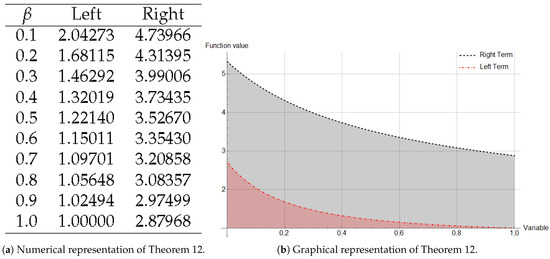
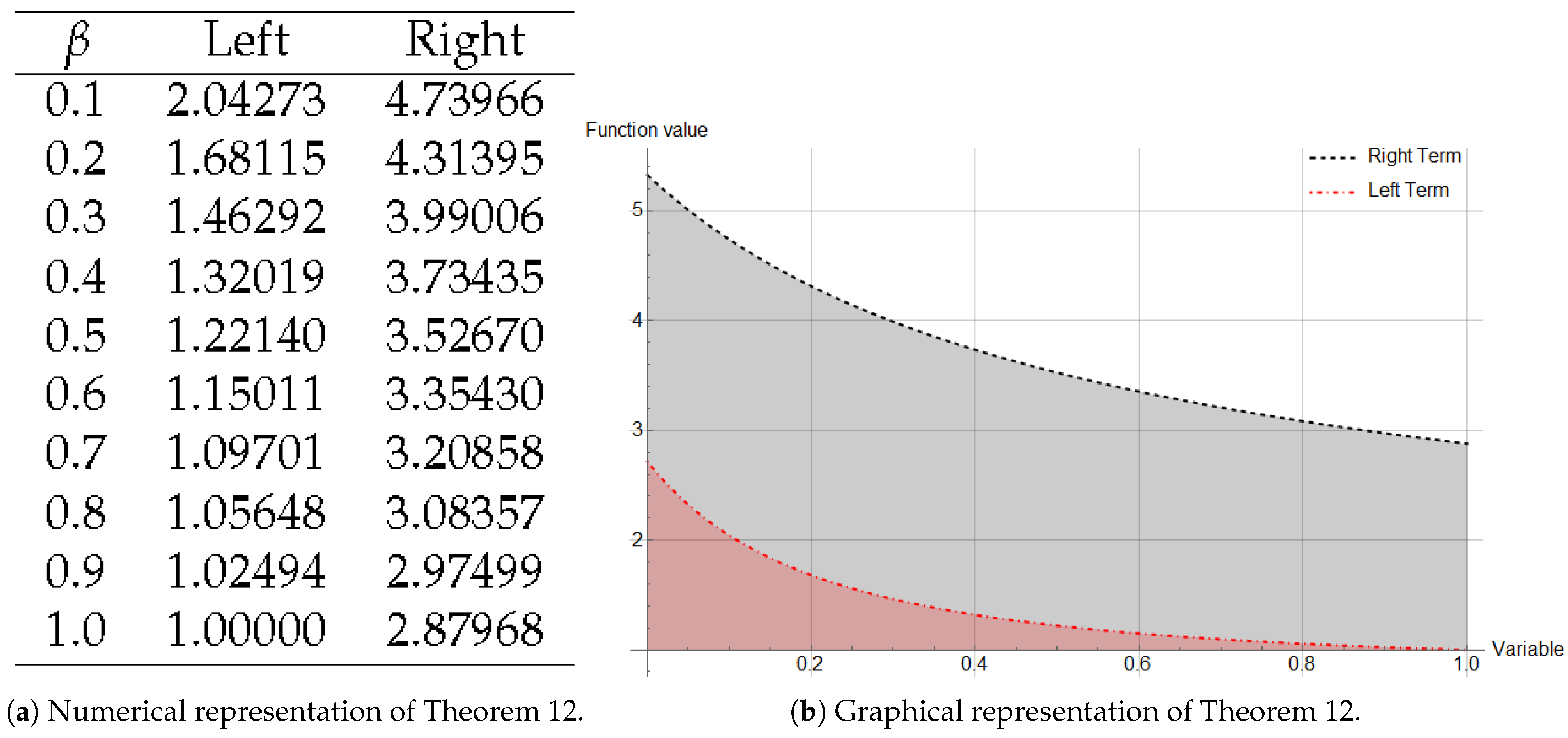
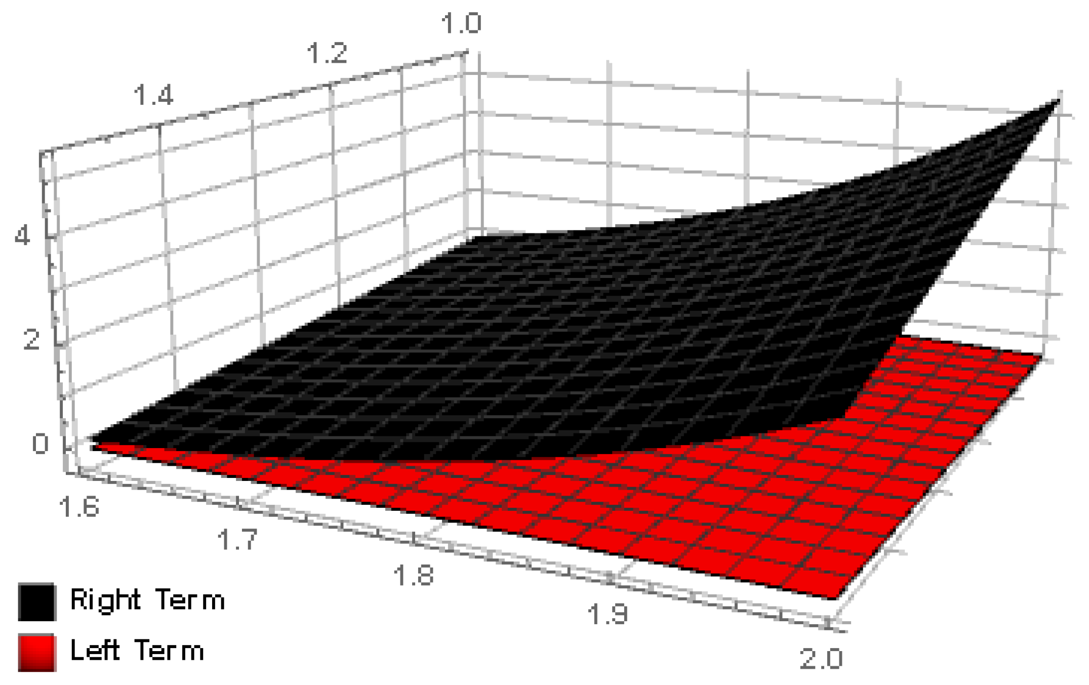
Analogously, taking $\vartheta =0$, $\upsilon =1$, $\mathrm{p}=2$, and $\mathrm{q}=2$ in Theorem 12, we compute the associated left- and right-hand expressions of the inequality.

$$\begin{array}{ll}& \mathit{Left}\mathit{Term}=exp\left\{{\displaystyle \frac{6+\beta +2{\beta }^2}{4+10\beta +4{\beta }^2}}-{\displaystyle \frac{1}{2}}\right\}\\ & \mathit{Right}\mathit{Term}=exp\left\{{\displaystyle \frac{1+\sqrt{3}}{\sqrt{8(2\beta +1)}}}+{\displaystyle \frac{1}{\sqrt{2(\beta +1)}}}\right\}\end{array}$$

These computations lead to the numerical results listed in Figure 5a and the graphical representation in Figure 5b.

The graphical illustrations verify the validity of the inequalities by showing that the curve corresponding to the right-hand side consistently lies above the curve corresponding to the left-hand side throughout the considered domain. Likewise, the tabulated numerical results demonstrate that the computed values of the left-hand side remain smaller than (or equal to, where applicable) the corresponding values of the right-hand side for all selected parameter values.

7. Applications

This section presents several applications that illustrate the scope and effectiveness of the proposed results. In particular, we demonstrate how the established inequalities can be utilized in the study of classical special means and in obtaining bounds for important special functions, thereby highlighting both the theoretical relevance and practical applicability of our framework.

7.1. Special Means

Special means, such as arithmetic, geometric, harmonic, and power means, play a central role in inequality theory and mathematical analysis, providing natural measures of central tendency and proportionality between quantities. They are widely used in optimization, numerical analysis, statistics, economics, and engineering to model averages, efficiencies, and equilibrium states. In this subsection, we apply our main results to establish new bounds and relationships for classical means, illustrating the usefulness of the developed inequalities in both theoretical investigations and practical computations.

Let $\mathrm{A}(\vartheta ,\upsilon )$, $\mathrm{W}(\vartheta ,\upsilon ,{\mathrm{k}}_1,{\mathrm{k}}_2)$, $\mathrm{G}(\vartheta ,\upsilon )$, $\mathrm{L}(\vartheta ,\upsilon )$, and ${\mathrm{M}}_{\mathrm{r}}(\vartheta ,\upsilon )$ denote the arithmetic, weighted arithmetic, geometric, logarithmic, and power means, respectively, defined as follows.

$$\begin{array}{ll}& A(\vartheta ,\upsilon )={\displaystyle \frac{\vartheta +\upsilon }{2}},\\ & W(\vartheta ,\upsilon ,{\mathrm{k}}_1,{\mathrm{k}}_2)={\displaystyle \frac{{\mathrm{k}}_1\vartheta +{\mathrm{k}}_2\upsilon }{{\mathrm{k}}_1+{\mathrm{k}}_2}},\\ & G(\vartheta ,\upsilon )=\sqrt{\vartheta \upsilon },\\ & L(\vartheta ,\upsilon )={\displaystyle \frac{\vartheta -\upsilon }{ln\vartheta -ln\upsilon }},\\ & M_{\mathrm{r}}(\vartheta ,\upsilon )={\left({\displaystyle \frac{{\vartheta }^{\mathrm{r}}+{\upsilon }^{\mathrm{r}}}{2}}\right)}^{{\displaystyle \frac{1}{\mathrm{r}}}}.\end{array}$$

Proposition 2.

The inequality

$$\begin{array}{ll}& \left|A^{\mathrm{m}}(\vartheta ,\upsilon )+{(\mathrm{m}+1)}^{-1}{\mathrm{L}}^{\mathrm{m}}(\vartheta ,\upsilon ){(lnG({\vartheta }^{-1},\upsilon ))}^{\mathrm{m}}-A^{-1}(-\vartheta ,\upsilon )\mathrm{L}({\vartheta }^{\mathrm{m}+1},{\upsilon }^{\mathrm{m}+1})lnG({\vartheta }^{-1},\upsilon )\right|\\ & \le {\displaystyle \frac{1}{3}}\left[A(-\vartheta ,\upsilon )M_{\mathrm{m}}^{\mathrm{m}}(\vartheta ,{\upsilon }^2)\right]\end{array}$$

holds for all $\vartheta ,\upsilon \in (0,\infty )$ and $\mathrm{m}\ge 2.$

Proof. 

The intended result is immediately obtained upon the application of the function $\mathrm{{\rm Y}}\left(\varkappa \right)=exp\left\{{\varkappa }^{\mathrm{m}}\right\}$ within the framework of Theorem 5. □

Example 5.

As depicted in Figure 6, Proposition 2 remains valid for multiple ranges of the parameters under consideration.

Proposition 3.

The inequality

$$\begin{array}{ll}& \left|{\displaystyle \frac{2{(ln\left(\frac{\upsilon }{\vartheta }\right))}^{\mathrm{m}}{\mathrm{L}}^{\mathrm{m}}(\upsilon ,\vartheta )-2^{\frac{1}{\mathrm{m}}}(2+\mathrm{m})M_{\mathrm{m}}^{\mathrm{m}}(-{\vartheta }^{1+\mathrm{m}},{\upsilon }^{1+\mathrm{m}})}{(1+\mathrm{m})(1+\mathrm{m})}}\right|\\ & \le {\displaystyle \frac{\mathrm{m}{\upsilon }^{\mathrm{m}-1}A(-\vartheta ,\upsilon )}{2}}+{\displaystyle \frac{\mathrm{m}{\left(ln\left(\frac{\upsilon }{\vartheta }\right)\right)}^{\mathrm{m}}{\mathrm{L}}^{\mathrm{m}}(\upsilon ,\vartheta )}{6}}+M_{\mathrm{m}}^{\mathrm{m}}(\vartheta ,\upsilon ),\end{array}$$

holds for all $\vartheta ,\upsilon \in (0,\infty )$ and $\mathrm{m}\ge 2.$

Proof. 

The intended result is immediately obtained upon the application of the function $\mathrm{{\rm Y}}\left(\varkappa \right)=exp\left\{{\varkappa }^{\mathrm{m}}\right\}$ within the framework of Theorem 7. □

Example 6.

As depicted in Figure 7, Proposition 2 remains valid for multiple ranges of the parameters under consideration.

7.2. Special Functions: Modified Bessel Function of Type I

The modified Bessel function of type I, originally introduced and systematically studied by Watson in his classical treatise on Bessel functions [54], occupies a central position in the theory of special functions. Special functions arise naturally in applied mathematics, physics, and engineering, where precise bounds and structural properties are indispensable for stability analysis, numerical approximation, and the modeling of physical phenomena. In particular, the modified Bessel function of the first kind appears prominently in problems involving heat conduction, diffusion processes, wave propagation, and certain statistical distributions.

Analytically, the modified Bessel function of type I emerges as a solution of the modified Bessel differential equation

$$\begin{array}{l}{\varkappa }^2{\mathrm{{\rm Y}}}^{″}\left(\varkappa \right)+\varkappa {\mathrm{{\rm Y}}}^{\prime }\left(\varkappa \right)-\left({\varkappa }^2+{\mathrm{k}}^2\right)\mathrm{{\rm Y}}\left(\varkappa \right)=0,\end{array}$$

where $\mathrm{k}\in \mathbb{R}$ denotes the order. The modified Bessel function of type I of order $\mathrm{k}$, denoted by ${\mathrm{J}}_{\mathrm{k}}\left(\varkappa \right)$, is defined through the convergent power series

$$\begin{array}{l}{\mathrm{J}}_{\mathrm{k}}\left(\varkappa \right)={\displaystyle \sum _{\mathrm{m}=0}^{\infty }}{\displaystyle \frac{{\left(\frac{\varkappa }{2}\right)}^{\mathrm{k}+2\mathrm{m}}}{\mathrm{m}!\mathsf{\Gamma }(\mathrm{k}+\mathrm{m}+1)}},\mathrm{where}\varkappa \in \mathrm{R}.\end{array}$$

Motivated by its broad applicability and analytical significance, we apply the inequalities established in the preceding sections to ${\mathrm{J}}_{\mathrm{k}}\left(\varkappa \right)$ in order to derive meaningful estimates, thereby illustrating the effectiveness and practical relevance of our results within the framework of special functions.

Motivated by the properties of the modified Bessel function of type I, we introduce the function ${\mathrm{{\rm Y}}}_{\mathrm{k}}:(0,\infty )\to (0,\infty )$ for each $\mathrm{k}\ge 5$, defined by

$$\begin{array}{l}{\mathrm{{\rm Y}}}_{\mathrm{k}}\left(\varkappa \right)={\varkappa }^{\mathrm{k}}{\mathrm{J}}_{\mathrm{k}}\left(\varkappa \right).\end{array}$$

$$\begin{array}{l}{\mathrm{{\rm Y}}}_{\mathrm{k}}^{\prime }\left(\varkappa \right)={\varkappa }^{\mathrm{k}}{\mathrm{J}}_{\mathrm{k}-1}\left(\varkappa \right).\end{array}$$

$$\begin{array}{l}{\mathrm{{\rm Y}}}_{\mathrm{k}}^{″}\left(\varkappa \right)={\varkappa }^{\mathrm{k}-1}{\mathrm{J}}_{\mathrm{k}-1}\left(\varkappa \right)+{\varkappa }^{\mathrm{k}}{\mathrm{J}}_{\mathrm{k}-2}\left(\varkappa \right).\end{array}$$

$$\begin{array}{l}{\mathrm{{\rm Y}}}_{\mathrm{k}}^{‴}\left(\varkappa \right)=3{\varkappa }^{\mathrm{k}-1}{\mathrm{J}}_{\mathrm{k}-2}\left(\varkappa \right)+{\varkappa }^{\mathrm{k}}{\mathrm{J}}_{\mathrm{k}-3}\left(\varkappa \right).\end{array}$$

$$\begin{array}{l}{\mathrm{{\rm Y}}}_{\mathrm{k}}^4\left(\varkappa \right)=3{\varkappa }^{\mathrm{k}-2}{\mathrm{J}}_{\mathrm{k}-2}\left(\varkappa \right)+6{\varkappa }^{\mathrm{k}-1}{\mathrm{J}}_{\mathrm{k}-3}\left(\varkappa \right)+{\varkappa }^{\mathrm{k}}{\mathrm{J}}_{\mathrm{k}-4}\left(\varkappa \right).\end{array}$$

$$\begin{array}{l}{\mathrm{{\rm Y}}}_{\mathrm{k}}^5\left(\varkappa \right)=15{\varkappa }^{\mathrm{k}-2}{\mathrm{J}}_{\mathrm{k}-3}\left(\varkappa \right)+10{\varkappa }^{\mathrm{k}-1}{\mathrm{J}}_{\mathrm{k}-4}\left(\varkappa \right)+{\varkappa }^{\mathrm{k}}{\mathrm{J}}_{\mathrm{k}-5}\left(\varkappa \right).\end{array}$$

Since ${\mathrm{{\rm Y}}}_{\mathrm{k}}^{\left(5\right)}\left(\varkappa \right)>0$ for all $\mathrm{k}\ge 5$ and $\varkappa >0$, it follows that ${\mathrm{{\rm Y}}}_{\mathrm{k}}^{‴}\left(\varkappa \right)$ is convex on $(0,\infty )$. Together with the conditions ${\mathrm{{\rm Y}}}_{\mathrm{k}}^{″}\left(0\right)=0$ and ${\mathrm{{\rm Y}}}_{\mathrm{k}}^{‴}\left(0\right)=0$, Lemma 3 implies that ${\mathrm{{\rm Y}}}_{\mathrm{k}}^{″}\left(\varkappa \right)$ is superquadratic. Moreover, a function is termed multiplicatively superquadratic whenever its logarithm is superquadratic. Observing that ${\mathrm{{\rm Y}}}_{\mathrm{k}}^{″}\left(\varkappa \right)=ln\left(exp\left\{{\mathrm{{\rm Y}}}_{\mathrm{k}}^{″}\left(\varkappa \right)\right\}\right),$ we conclude that $exp\left\{{\mathrm{{\rm Y}}}_{\mathrm{k}}^{″}\left(\varkappa \right)\right\}$ is multiplicatively superquadratic.

Proposition 4.

The inequality

$$\begin{array}{ll}& |exp\{{\left({\displaystyle \frac{\vartheta +\upsilon }{2}}\right)}^{\mathrm{k}-1}{\mathrm{J}}_{\mathrm{k}-1}\left({\displaystyle \frac{\vartheta +\upsilon }{2}}\right)+{\left({\displaystyle \frac{\vartheta +\upsilon }{2}}\right)}^{\mathrm{k}}{\mathrm{J}}_{\mathrm{k}-2}\left({\displaystyle \frac{\vartheta +\upsilon }{2}}\right)\\ & +{\displaystyle \frac{1}{\upsilon -\vartheta }}\left(2\left({\left({\displaystyle \frac{\upsilon -\vartheta }{2}}\right)}^{\mathrm{k}}{\mathrm{J}}_{\mathrm{k}-1}\left({\displaystyle \frac{\upsilon -\vartheta }{2}}\right)\right)-{\vartheta }^{\mathrm{k}}{\mathrm{J}}_{\mathrm{k}-1}\left(\vartheta \right)-{\upsilon }^{\mathrm{k}}{\mathrm{J}}_{\mathrm{k}-1}\left(\upsilon \right)\right)\left\}\right|\\ & \le exp\left\{{\displaystyle \frac{\upsilon -\vartheta }{4}}{\left(3{\vartheta }^{\mathrm{k}-1}{\mathrm{J}}_{\mathrm{k}-2}\left(\vartheta \right)+{\vartheta }^{\mathrm{k}}{\mathrm{J}}_{\mathrm{k}-3}\left(\vartheta \right)+{\left(3{\upsilon }^{\mathrm{k}-1}{\mathrm{J}}_{\mathrm{k}-2}\left(\upsilon \right)+{\upsilon }^{\mathrm{k}}{\mathrm{J}}_{\mathrm{k}-3}\left(\upsilon \right)\right)}^2\right)}^{{\displaystyle \frac{1}{3}}}\right\}\end{array}$$

holds for all $\vartheta ,\upsilon \in (0,\infty )$ such that $\vartheta <\upsilon$ and $\mathrm{k}\ge 5$.

Proof. 

The intended result is immediately obtained upon the application of the function $\mathrm{{\rm Y}}\left(\varkappa \right)=exp\left\{{\mathrm{{\rm Y}}}_{\mathrm{k}}^{″}\left(\varkappa \right)\right\}$ within the framework of Theorem 5. □

Example 7.

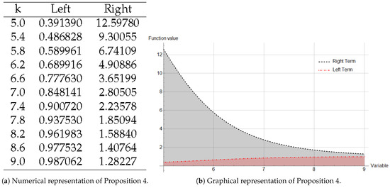
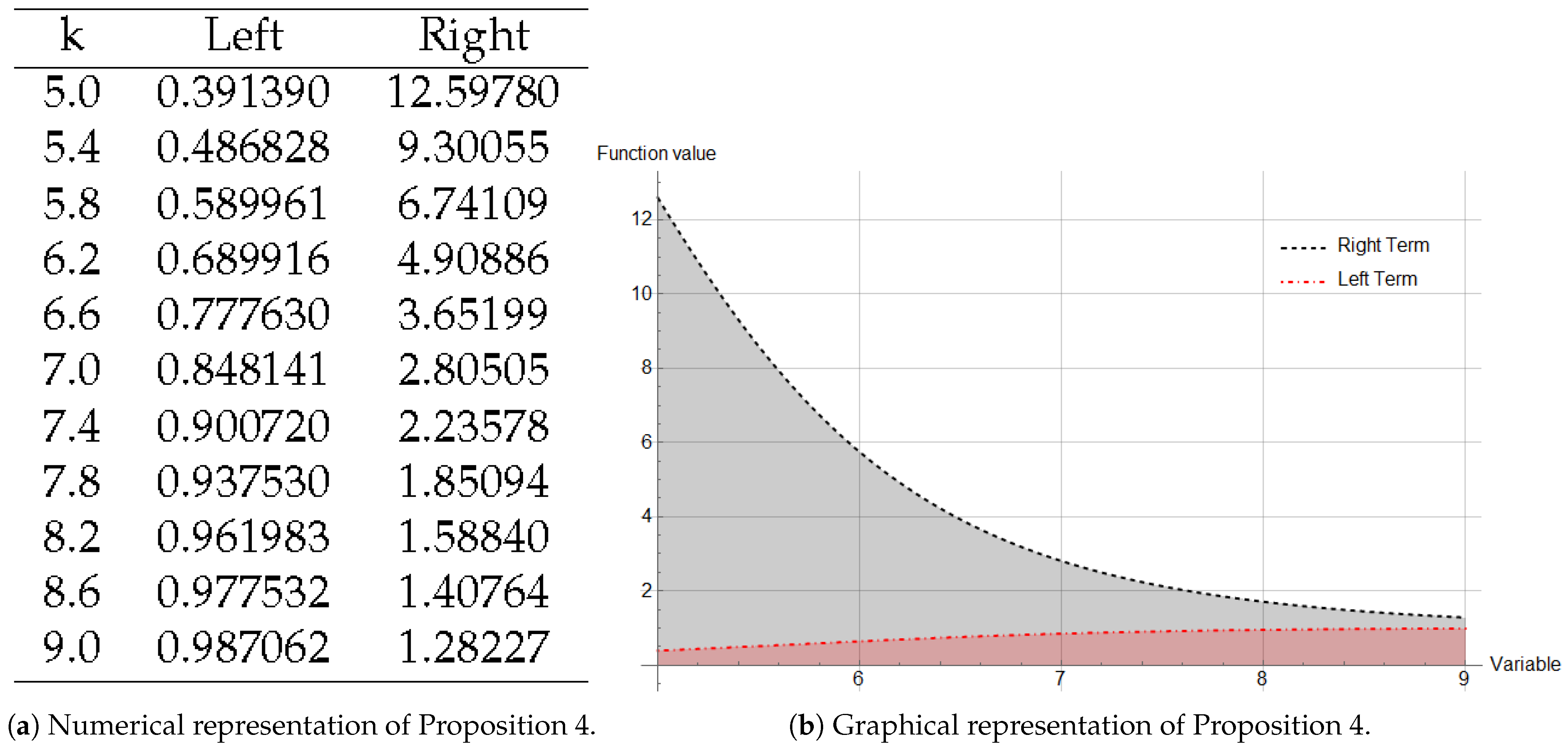
We perform numerical computations and graphical visualizations for various parameter choices in Proposition 4 to demonstrate the applicability of our findings. Specifically, with $\vartheta =1$, $\upsilon =2$, and $\mathrm{k}\in [5,9]$, we obtain the numerical results listed in Figure 8a and their corresponding graphical representation in Figure 8b.

Proposition 5.

The inequality

$$\begin{array}{ll}& \left|exp\left\{{\displaystyle \frac{{\upsilon }^{\mathrm{k}}{\mathrm{J}}_{\mathrm{k}-1}\left(\upsilon \right)-{\vartheta }^{\mathrm{k}}{\mathrm{J}}_{\mathrm{k}-1}\left(\vartheta \right)}{\upsilon -\vartheta }}+2{(\upsilon -\vartheta )}^{\mathrm{k}-2}{\mathrm{J}}_{\mathrm{k}}(\upsilon -\vartheta )\right\}\right|\\ & \le exp\{3\left(3{\upsilon }^{\mathrm{k}-1}{\mathrm{J}}_{\mathrm{k}-2}\left(\upsilon \right)+{\upsilon }^{\mathrm{k}}{\mathrm{J}}_{\mathrm{k}-3}\left(\upsilon \right)\right)+2\left(3{(\upsilon -\vartheta )}^{\mathrm{k}-1}{\mathrm{J}}_{\mathrm{k}-2}(\upsilon -\vartheta )+{(\upsilon -\vartheta )}^{\mathrm{k}}{\mathrm{J}}_{\mathrm{k}-3}(\upsilon -\vartheta )\right)\\ & +{\displaystyle \frac{1}{2}}\left({\vartheta }^{\mathrm{k}-1}{\mathrm{J}}_{\mathrm{k}-1}\left(\vartheta \right)+{\vartheta }^{\mathrm{k}}{\mathrm{J}}_{\mathrm{k}-2}\left(\vartheta \right)+{\upsilon }^{\mathrm{k}-1}{\mathrm{J}}_{\mathrm{k}-1}\left(\upsilon \right)+{\upsilon }^{\mathrm{k}}{\mathrm{J}}_{\mathrm{k}-2}\left(\upsilon \right)\right)\}\end{array}$$

holds for all $\vartheta ,\upsilon \in (0,\infty )$ such that $\vartheta <\upsilon$ and $\mathrm{k}\ge 5$.

Proof. 

The intended result is immediately obtained upon the application of the function $\mathrm{{\rm Y}}\left(\varkappa \right)=exp\left\{{\mathrm{{\rm Y}}}_{\mathrm{k}}^{″}\left(\varkappa \right)\right\}$ within the framework of Theorem 7. □

Example 8.

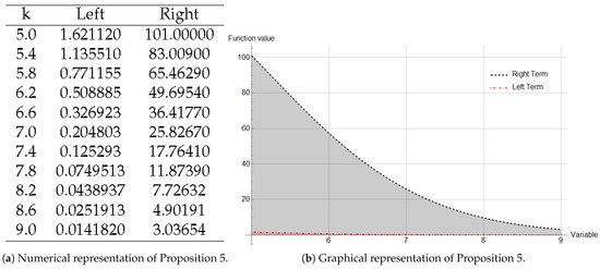
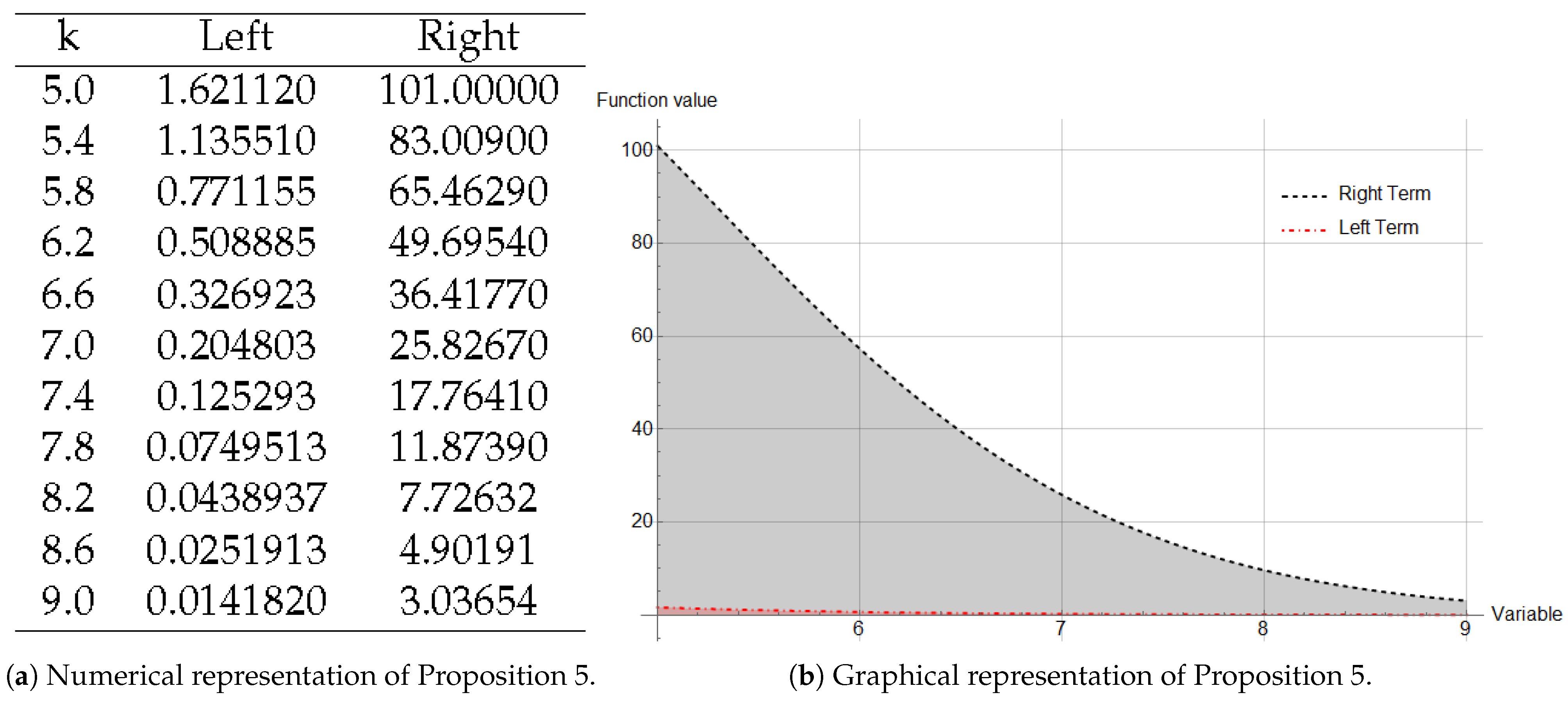
To illustrate the effectiveness of Proposition 5, we conduct representative numerical calculations and visualize the outcomes graphically for selected parameters. Setting $\vartheta =1$, $\upsilon =2$, and $\mathrm{k}$ within the interval $[5,9]$, the resulting values are compiled in Figure 9a, and their graphical representation is displayed in Figure 9b.

8. Conclusions

The present paper proposes a new Petrovič-type inequality and related integral identities for multiplicatively superquadratic functions in the context of multiplicative calculus. To the best of the authors’ knowledge, for the first time, such midpoint- and trapezoid-type inequalities for these classes of functions, including the fractional ones by means of the multiplicative Riemann–Liouville fractional operators, are derived. The results obtained in the paper are supported by numerical and graphical examples, demonstrating the importance and application of the results obtained.

Future Research Directions

The results established in this paper provide a foundation for the development of further inequalities in multiplicative calculus, including multiplicative analogues of Ostrowski-, Simpson-, Boole-, Newton-, and Maclaurin-type inequalities. Moreover, the obtained Petrovič-type inequality and related results can be extended to the framework of multiplicative fractional calculus by employing various fractional integral operators, such as conformable, tempered, Sarikaya-type, proportional Caputo-hybrid, and exponential-kernel multiplicative operators. Further generalizations may also be achieved through multiplicative integral operators and multiple-integral formulations in higher-dimensional settings. Such extensions are expected to yield new inequalities for broader classes of multiplicatively convex and multiplicatively superquadratic functions, thereby enriching the theory of multiplicative calculus and opening new directions for future research.

References

- Hadamard, J. Etude sur les proprietes des fonctions entieres et en particulier d’une fonction considree par Riemann. J. Mathémat. Pures Appli. 1893, 58, 171–215. [Google Scholar]
- Dragomir, S.S.; Agarwal, R.P. Two inequalities for differentiable mappings and applications to special means of real numbers and to trapezoidal formula. Appl. Math. Lett. 1998, 11, 91–95. [Google Scholar] [CrossRef] [Scilit]
- Kirmaci, U.S. Inequalities for differentiable mappings and applications to special means of real numbers and to midpoint formula. Appl. Math. Comput. 2004, 147, 137–146. [Google Scholar] [CrossRef] [Scilit]
- Abramovich, S.; Jameson, G.; Sinnamon, G. Refining Jensen’s inequality. Bull. Math. Société Sci. Math. Roum. 2004, 47, 3–14. [Google Scholar]
- Abramovich, S.; Jameson, G.; Sinnamon, G. Inequalities for averages of convex and superquadratic functions. J. Inequal. Pure Appl. Math. 2004, 5, 91. [Google Scholar]
- Krnić, M.; Moradi, H.R.; Sababheh, M. On logarithmically superquadratic functions. Mediterr. J. Math. 2023, 20, 2–18. [Google Scholar] [CrossRef] [Scilit] [PubMed]
- Bradanović, S. More accurate majorization inequalities obtained via superquadraticity and convexity with application to entropies. Mediterr. J. Math. 2021, 18, 79. [Google Scholar] [CrossRef] [Scilit]
- Alomari, M.W.; Chesneau, C. On h-superquadratic functions. Afr. Mat. 2022, 33, 41. [Google Scholar] [CrossRef] [Scilit]
- Butt, S.I.; Khan, D. Integral inequalities of h-superquadratic functions and their fractional perspective with applications. Math. Methods Appl. Sci. 2025, 48, 1952–1981. [Google Scholar] [CrossRef] [Scilit]
- Butt, S.I.; Khan, D. Superquadratic function and its applications in information theory via interval calculus. Chaos Solitons Fractals 2025, 190, 115748. [Google Scholar] [CrossRef] [Scilit]
- Grossman, M.; Katz, R. Non-Newtonian Calculus; Lee Press: Pigeon Cove, MA, USA, 1972. [Google Scholar]
- Bashirov, A.E.; Kurpinar, E.M.; Özyapici, A. Multiplicative calculus and its applications. J. Math. Anal. Appl. 2008, 337, 36–48. [Google Scholar] [CrossRef] [Scilit]
- Has, A.; Yilmaz, B.; Yildirim, H. A non-Newtonian perspective on multiplicative Lorentz–Minkowski space . Math. Methods Appl. Sci. 2024, 47, 13875–13888. [Google Scholar] [CrossRef] [Scilit]
- Göktaş, S.; Kemaloğlu, H.; Yilmaz, E. Multiplicative conformable fractional Dirac system. Turk. J. Math. 2022, 46, 973–990. [Google Scholar] [CrossRef] [Scilit]
- Boruah, K.; Hazarika, B. Application of geometric calculus in numerical analysis and difference sequence spaces. J. Math. Anal. Appl. 2017, 449, 1265–1285. [Google Scholar] [CrossRef] [Scilit]
- Has, A.; Yilmaz, B. Non-Newtonian conics in multiplicative analytic geometry. Turk. J. Math. 2024, 48, 976–994. [Google Scholar]
- Berkane, A.; Meftah, B.; Lakhdari, A. Right–Radau-type inequalities for multiplicative differentiable s-convex functions. J. Appl. Math. Inform. 2024, 42, 785–800. [Google Scholar] [CrossRef]
- Latif, M.A.; Kalsoom, H.; Abidin, M.Z. Hermite–Hadamard-Type inequalities involving harmonically convex function via the Atangana–Baleanu fractional integral operator. Symmetry 2022, 14, 1774. [Google Scholar] [CrossRef] [Scilit]
- Mumcu, İ.; Set, E.; Akdemir, A.O.; Jarad, F. New extensions of Hermite-Hadamard inequalities via gener alized proportional fractional integral. Numer. Methods Partial Differ. Equ. 2024, 40, e22767. [Google Scholar] [CrossRef] [Scilit]
- Han, J.F.; Mohammed, P.O.; Zeng, H.D. Generalized fractional integral inequalities of Hermite-Hadamard- type for a convex function. Open Math. 2020, 18, 794–806. [Google Scholar] [CrossRef] [Scilit]
- Chen, H.; Katugampola, U.N. Hermite-Hadamard and Hermite-Hadamard-Fejér type inequalities for generalized fractional integrals. J. Math. Anal. Appl. 2017, 446, 1274–1291. [Google Scholar] [CrossRef] [Scilit]
- Balenau, D.; Ferrandez, A.; Akgül, A. On a fractional operator combining proportional and classical differintegrals. Mathematics 2020, 8, 360. [Google Scholar] [CrossRef] [Scilit]
- Dragomir, S.S. Hermite-Hadamard type inequalities for generalized Riemann-Liouville fractional integrals of h-convex functions. Math. Methods Appl. Sci. 2021, 44, 2364–2380. [Google Scholar] [CrossRef] [Scilit]
- Bohner, M.; Kashuri, A.; Mohammed, P.O.; Valdés, J.E.N. Hermite-Hadamard-type inequalities for conformable integrals. Hacet. J. Math. Stat. 2022, 51, 775–786. [Google Scholar] [CrossRef] [Scilit]
- Li, L.N.; Li, Y.Z.; Huang, Q.D. Fractional order Chebyshev cardinal functions for solving two classes of fractional differential equations. Eng. Lett. 2022, 30, 208–213. [Google Scholar]
- Alomari, A.K.; Massoun, Y. Numerical solution of time fractional coupled Korteweg–de Vries equation with a Caputo fractional derivative in two parameters. IAENG Int. J. Comput. Sci. 2023, 50, 388–393. [Google Scholar]
- Kankhunthodi, K.; Kongratana, V.; Numsomran, A.; Tipsuwanporn, V. Self-balancing robot control using fractional-order PID controller. In Proceedings of the International MultiConference of Engineers and Computer Scientists, Hong Kong, China, 13–15 March 2019; pp. 77–82. [Google Scholar]
- Abdeljawad, T.; Grossman, M. On geometric fractional calculus. J. Semigroup Theory Appl. 2016, 2016, 2. [Google Scholar] [CrossRef] [Scilit]
- Meftah, B.; Lakhdari, A.; Wedad, S.; Benchettah, D.C. Companion of Ostrowski inequality for multiplicatively convex functions. Sahand Commun. Math. Anal. 2024, 21, 289–304. [Google Scholar] [CrossRef]
- Özcan, S. Simpson, midpoint, and trapezoid-type inequalities for multiplicatively s-convex functions. Demonstr. Math. 2025, 58, 20240060. [Google Scholar] [CrossRef] [Scilit]
- Mateen, A.; Zhang, Z.Y.; Toseef, M.; Ali, M.A. A new version of Boole’s formula type inequalities in multiplicative calculus with application to quadrature formula. Bull. Belg. Math. Soc. 2024, 31, 541–562. [Google Scholar] [CrossRef] [Scilit]
- Chasreechai, S.; Ali, M.A.; Naowarat, S.; Sitthiwirattham, T.; Nonlaopon, K. On some Simpson’s and Newton’s type of inequalities in multiplicative calculus with applications. AIMS Math. 2023, 8, 3885–3896. [Google Scholar] [CrossRef] [Scilit]
- Meftah, B. Maclaurin type inequalities for multiplicatively convex functions. Proc. Am. Math. Soc. 2023, 151, 2115–2125. [Google Scholar] [CrossRef] [Scilit]
- Xie, J.Q.; Ali, M.A.; Sitthiwirattham, T. Some new midpoint and trapezoidal type inequalities in multiplicative calculus with applications. Filomat 2023, 37, 6665–6675. [Google Scholar] [CrossRef] [Scilit]
- Budak, H.; Özçelik, K. On Hermite–Hadamard type inequalities for multiplicative fractional integrals. Miskolc Math. Notes 2020, 21, 91–99. [Google Scholar] [CrossRef] [Scilit]
- Boulares, H.; Meftah, B.; Moumen, A.; Shafqat, R.; Saber, H.; Alraqad, T.; Ali, E.E. Fractional multiplicative Bullen-type inequalities for multiplicative differentiable functions. Symmetry 2023, 15, 451. [Google Scholar] [CrossRef] [Scilit]
- Merad, M.; Meftah, B.; Moumen, A.; Bouye, M. Fractional Maclaurin-type inequalities for multiplicatively convex functions. Fractal Fract. 2023, 7, 879. [Google Scholar] [CrossRef] [Scilit]
- Lakhdari, A.; Benchettah, D.C.; Meftah, B. Fractional multiplicative Newton-type inequalities for multiplicative s-convex positive 680 functions with application. J. Comput. Appl. Math. 2025, 465, 116600. [Google Scholar] [CrossRef] [Scilit]
- Almatrafi, M.B.; Saleh, W.; Lakhdari, A.; Jarad, F.; Meftah, B. On the multiparameterized fractional multiplicative integral inequalities. J. Inequal. Appl. 2024, 2024, 52. [Google Scholar] [CrossRef] [Scilit]
- Du, T.S.; Long, Y. The multi-parameterized integral inequalities for multiplicative Riemann–Liouville fractional integrals. J. Math. Anal. Appl. 2025, 541, 128692. [Google Scholar] [CrossRef] [Scilit]
- Budak, H.; Ergün, B.B. On multiplicative conformable fractional integrals: Theory and applications. Bound. Value Probl. 2025, 2025, 30. [Google Scholar] [CrossRef] [Scilit]
- Fu, H.; Peng, Y.; Du, T.S. Some inequalities for multiplicative tempered fractional integrals involving the λ-incomplete gamma functions. AIMS Math. 2021, 6, 7456–7478. [Google Scholar] [CrossRef] [Scilit]
- Kashuri, A.; Sahoo, S.K.; Aljuaid, M.; Tariq, M.; Sen, M.D.L. Some new Hermite–Hadamard type inequalities pertaining to generalized multiplicative fractional integrals. Symmetry 2023, 15, 868. [Google Scholar] [CrossRef] [Scilit]
- Umar, M.; Butt, S.I.; Seol, Y. Hybrid fractional integral inequalities in multiplicative calculus with applications. Fractals 2025, 33, 2550019. [Google Scholar] [CrossRef] [Scilit]
- Peng, Y.; Fu, H.; Du, T.S. Estimations of bounds on the multiplicative fractional integral inequalities having exponential kernels. Commun. Math. Stat. 2024, 12, 187–211. [Google Scholar] [CrossRef] [Scilit]
- Zhou, Z.Y.; Du, T.S. Analytical properties and related inequalities derived from multiplicative Hadamard k-fractional integrals. Chaos Solitons Fractals 2024, 189, 115715. [Google Scholar] [CrossRef] [Scilit]
- Long, Y.; Du, T.S. Analysis on multiplicative k-Atangana–Baleanu fractional integrals with application to various Mercer-type 698 inequalities. Fractals 2025, 33, 2550003. [Google Scholar] [CrossRef] [Scilit]
- Petrović, M. Sur une fonctionnelle. Publ. Math. Univ. Belgrade 1932, 1, 146–149. [Google Scholar]
- Pečarić, J.E. On the Petrović inequality for convex functions. Glas. Mat. 1983, 18, 77–85. [Google Scholar]
- Butt, S.I.; Pečarić, J.; Ur Rehman, A. Exponential convexity of Petrović and related functional. J. Inequal. Appl. 2011, 2011, 89. [Google Scholar] [CrossRef] [Scilit]
- Rehman, A.U.; Mudessir, M.; Fazal, H.T.; Farid, G. Petrović’s inequality on coordinates and related results. Cogent Math. 2016, 3, 1227298. [Google Scholar] [CrossRef] [Scilit]
- Rehman, A.U.; Farid, G.; Mishra, V.N. Generalized convex function and associated Petrović’s inequality. Int. J. Anal. Appl. 2019, 17, 122–131. [Google Scholar] [CrossRef]
- Butt, S.I.; Khan, D.; Tipurić-Spužević, S.; Seol, Y. Generalized Petrović inequality and its related estimations in superquadraticity on the fractal space with applications. Fractals 2025, 33, 2550086. [Google Scholar] [CrossRef] [Scilit]
- Watson, G.N. A Treatise on the Theory of Bessel Functions; Cambridge University Press: Cambridge, UK, 1944. [Google Scholar]
Disclaimer/Publisher’s Note: The statements, opinions and data contained in all publications are solely those of the individual author(s) and contributor(s) and not of MDPI and/or the editor(s). MDPI and/or the editor(s) disclaim responsibility for any injury to people or property resulting from any ideas, methods, instructions or products referred to in the content. |
© 2026 by the authors. Licensee MDPI, Basel, Switzerland. This article is an open access article distributed under the terms and conditions of the Creative Commons Attribution (CC BY) license.