


Abstract
Rainfall-index-based disaster insurance is an efficient approach to mitigating hydrometeorological losses. However, conventional premium pricing models generally assume memoryless stochastic dynamics that do not fully capture the long-range dependence inherent in rainfall data. This study develops a hydrometeorological disaster insurance model within a fractional Black–Scholes framework to incorporate long-memory effects. The model is formulated using fractional differential equations and solved semi-analytically by integrating the Daftardar–Jafari Method (DJM) with the Kashuri–Fundo (KF) transform, yielding a closed-form solution expressed in terms of the Mittag–Leffler function. The proposed contract is structured as parametric rainfall insurance with a multi-layer payout mechanism based on percentiles corresponding to minor, moderate, and severe housing damage. The results show that variations in the fractional-order parameter significantly affect premium estimation. In particular, recovers the classical model and tends to generate higher premiums than the fractional model with , whereas the model with yields lower premiums. These findings indicate that fractional-order parameterization can accommodate diverse risk characteristics and policyholders’ economic capacities, enabling more adaptive, risk-sensitive premium structures. In line with SDG 13 (Climate Action), the proposed framework offers a climate-responsive disaster-mitigation strategy through accessible, actuarially relevant insurance design.
Keywords:
hydrometeorological disaster insurance; rainfall index-based; fractional Black–Scholes model; climate change; SDG 13 (Climate Action) MSC:
34A08; 60G22; 91B30; 91G80; 62P05; 86A08
1. Introduction
Hydrometeorological risks, such as floods and droughts, are strongly influenced by high rainfall variability, both spatially and temporally. High-intensity rainfall can trigger floods that directly damage infrastructure and settlements, while prolonged low rainfall can lead to droughts that disrupt community livelihoods [1,2]. Within the global framework, efforts to mitigate these risks align with achieving SDG target 13, which emphasizes strengthening resilience and adaptive capacity to climate-related disasters. In recent decades, the increase in extreme rainfall events has amplified risk exposure to physical assets, including residential buildings, particularly in areas with high vulnerability [3,4]. Climate projections further indicate that extreme wet events will continue to intensify throughout the 21st century, while certain regions simultaneously experience longer dry periods, increasing dual exposure to both flood and drought risks [5,6,7].
From a modeling perspective, rainfall is a stochastic process because it is influenced by complex, uncertain atmospheric dynamics. Therefore, stochastic approaches are important in representing rainfall variability and in evaluating hydrometeorological risks more realistically. In this context, the integration of weather statistics and financial models has evolved through the concept of weather derivatives, as proposed by Jewson and Brix (2005) and Alaton et al. (2002) [8,9]. One of the models widely used within this framework is the Black–Scholes model, introduced by Black and Scholes (1973) and further developed in modern derivatives literature by Hull (2018) [10,11]. In the context of rainfall-index-based insurance, the contract structure can be represented analogously to a financial option, so that the premium can be expressed as the discounted expected value of the payoff.
However, the classical Black–Scholes approach has limitations in representing the complex dynamics of rainfall. This model is based on a geometric Brownian motion process that is memoryless and therefore cannot capture long-range dependence, which frequently appears in hydrometeorological data. To address this limitation, a fractional approach based on the concept of fractional Brownian motion by Mandelbrot & Van Ness (1968) is utilized [12]. This concept was later formalized within the framework of stochastic calculus by Biagini et al. (2008) and further developed by Bender & Viitasaari (2016) [13,14].
The development of the fractional Black–Scholes model has been further extended in various studies. Necula (2002) showed that models based on fractional Brownian motion with a Hurst parameter can capture long-range dependence that classical models cannot [15]. This is reinforced by Comte and Renault (1998), who identified memory structures in financial market volatility [16], and by the development of fractional stochastic calculus by Hu and Øksendal (2003), which serves as the mathematical foundation for memory-based financial models [17]. Furthermore, Chen et al. (2015) developed the formulation of fractional Black–Scholes partial differential equations and demonstrated their flexibility in representing complex stochastic systems [18], while He and Lin (2021) showed that fractional approaches are able to improve accuracy in modeling derivative pricing in systems with memory-dependent volatility [19].
In the hydrometeorological context, Lovejoy and Mandelbrot (1985) highlighted that rainfall processes exhibit fractional characteristics through the Noah effect and Hurst law, indicating the presence of persistence and long-range dependence that cannot be adequately captured by classical stochastic models [20]. This observation provides a strong theoretical basis for adopting fractional approaches in rainfall-based risk modeling, particularly in applications where memory effects play an important role in determining future dynamics.
To obtain analytical insights from such models, a variety of semi-analytical techniques have been developed for solving fractional differential equations. Among these, the DJM, introduced by Daftardar-Gejji and Jafari (2006), offers an iterative framework capable of generating convergent series solutions without the need for linearization or discretization [21]. Integral transform techniques have also been extensively employed to simplify the treatment of fractional operators and improve analytical tractability [22]. More recently, the KF transform has emerged as a promising alternative for systematically handling fractional differential systems [23]. Furthermore, advances in fractional differential equation theory have extended the analysis of existence, uniqueness, and controllability to increasingly sophisticated settings involving -Hilfer operators and stochastic integro-differential systems, reflecting the growing mathematical maturity and applicability of fractional frameworks in risk-sensitive modeling [24]. These developments motivate integrating the DJM and the Kashuri–Fundo transform in the present study to derive a semi-analytical solution to the fractional Black–Scholes model while preserving its underlying memory characteristics.
In line with these developments, research on determining premiums for rainfall-index-based insurance using the Black–Scholes model has made significant progress, as demonstrated by Kalfin et al. (2022) and Purwandari et al. (2024) [25,26]. Efforts to integrate fractional approaches remain relatively limited, as seen in the study by Azahra et al. (2025), which developed a fractional Black–Scholes model for rainfall index-based premium determination but was still limited to the agricultural context [27,28]. These findings indicate that developing fractional models in the broader context of disaster insurance remains an open research opportunity.
The determination of insurance premiums and compensation thresholds in this study employs the Historical Burn Analysis (HBA) method, which transforms historical climate observations into risk indices by directly utilizing past disaster records to estimate trigger and exit values. This approach has been widely adopted in weather index-based insurance due to its objectivity and transparency in linking measurable climatic variables to compensation mechanisms [25,29]. However, HBA alone is insufficient for capturing rainfall’s stochastic dynamics; it requires integration with a probabilistic pricing framework to produce actuarially sound premium estimates [25,27,30]. This gap motivates combining HBA with the fractional Black–Scholes model as the core methodological contribution of this study.
In addition, approaches that simultaneously model the risks of excess rainfall (floods) and rainfall deficit (droughts) within a unified framework remain relatively limited, even though the characteristics of extreme rainfall exhibit complex long-range dependence and temporal persistence patterns associated with climate variability and hydrometeorological processes [31,32,33,34]. Therefore, there remains a need to develop approaches that are not only capable of representing rainfall dynamics more realistically through fractional Black–Scholes models, but also of integrating multi-risk modeling and solution strategies based on a more comprehensive combination of methods [27,35,36,37,38]. From a risk financing perspective, parametric insurance schemes based on objectively measurable indices have been recognized as a promising complement to conventional indemnity-based insurance, particularly in contexts where post-disaster recovery funds are limited and transparent, pre-arranged claim mechanisms are needed [39]. This further motivates the development of mathematically rigorous index-based insurance frameworks that provide actuarially sound, verifiable premium structures.
To address these limitations, this study develops a parametric disaster insurance model based on rainfall indices, using a fractional Black–Scholes framework to capture long-memory effects. The research is structured as follows. First, the current state of hydrometeorological disaster insurance research is examined, identifying the gap in models that simultaneously address long-range dependence, multi-risk scenarios (flood and drought), and semi-analytical solvability. Second, the required mathematical theories are presented, encompassing fractional calculus (Caputo derivative), the KF integral transform, the Mittag–Leffler function, the fractional Black–Scholes framework, and the DJM. Third, the proposed method is formulated as a parametric rainfall-index insurance model with a multi-layer payout structure, solved semi-analytically using the combined DJM–KF approach. Finally, the feasibility and advantages of the proposed method are demonstrated through a case study in Bandung, West Java, comparing fractional and standard Black–Scholes premiums and evaluating compensation mechanisms via the HBA method.
The main contributions of this study are as follows. First, the fractional Black–Scholes equation is solved semi-analytically using a novel combination of the DJM and the KF transform, yielding a general closed-form solution expressed in terms of the Mittag–Leffler function. Second, a unified parametric insurance model is developed that simultaneously addresses flood and drought risk within a single framework, with a multi-layer compensation structure differentiated by housing damage severity. Third, the study provides empirical evidence that the fractional-order parameter can be calibrated to match the long-memory characteristics of observed rainfall data, enabling adaptive and inclusive premium structures consistent with SDG 13 objectives. Thus, this study not only contributes to the development of mathematical models in index-based insurance but also has practical implications for supporting hydrometeorological disaster risk mitigation strategies and strengthening climate change adaptation efforts in line with the achievement of SDG 13.
2. Mathematical Preliminaries and Notation
This section introduces the fundamental mathematical concepts used throughout this study. Fractional calculus extends classical calculus by allowing derivatives and integrals of non-integer order, enabling the modeling of systems with memory and hereditary properties. In the context of hydrometeorological modeling, the utility of fractional calculus lies in its ability to represent persistent memory effects inherent in rainfall processes, which classical stochastic models based on standard Brownian motion fail to capture. The following subsections present the key definitions and properties of the Caputo fractional derivative, the KF integral transform, and the Mittag–Leffler function, which collectively form the mathematical foundation of the fractional Black–Scholes framework developed in this study.
This capability has been demonstrated in hydrological modeling, where fractional-order operators based on the Caputo derivative have been applied to represent memory effects and long-term dependencies across key components of the water cycle, including rainfall, surface water, and groundwater dynamics, yielding improved accuracy compared to classical integer-order approaches [40].
Definition 1
([22]). The Caputo fractional derivative, for a function to
of real order
, where
, satisfies the following condition:
The Caputo fractional derivative is selected in this study for three principal reasons. First, unlike the Riemann–Liouville derivative, the Caputo derivative allows initial conditions to be expressed in terms of classical integer-order derivatives, which carry direct physical interpretations and are consistent with standard observational data [22,41]. Second, the Caputo operator is well-suited for modeling memory effects in systems where the initial state is known, as in rainfall-based insurance, where historical data serve as the starting point for premium computation. Third, the Caputo derivative commutes with the KF transform in a manner that yields a tractable algebraic structure (Theorem 1), enabling the systematic derivation of the DJM–KF solution scheme. While other operators, such as the Hilfer, -Caputo, and -Hilfer derivatives, offer greater generality through interpolation parameters or kernel flexibility, they introduce additional complexity that is not required given the data-driven estimation of in this study. Nevertheless, the DJM iterative decomposition framework in Section 3 is operator-agnostic in structure: provided the chosen fractional derivative admits a compatible integral transform with a known convolution property analogous to Theorem 1, the solution procedure can be adapted accordingly. This extensibility is noted as a direction for future research.
Consider the following fractional differential equation with the Caputo derivative:
with the initial condition where denotes the fractional derivative operator (in the Caputo sense), is a linear operator, is a nonlinear operator, represents the nonhomogeneous term, and is the unknown function to be determined [22,35,41].
Furthermore, the integral transform used in this study is the KF Transform, which is defined as follows [23]:
The inverse of the KF transform is denoted by
For as a fractional number, the KF transform satisfies [23]:
thus, its inverse is given by
Theorem 1
([23]). The following property of the KF transform with respect to the Caputo fractional derivative holds:
This transform possesses properties with respect to the Caputo fractional derivative that enable the systematic solution of fractional differential equations.
Definition 2
([22]). The Mittag–Leffler function plays an important role in representing solutions of fractional differential equations and is defined as follows:
This function is a generalization of the exponential function, since for
it holds that [22,42]:
Since the exponential function constitutes an essential component of the classical Black–Scholes formulation, the standard Black–Scholes model is briefly reviewed before introducing its fractional counterpart. The classical Black–Scholes model is one of the fundamental frameworks in financial mathematics used to determine derivative prices based on the stochastic dynamics of the underlying variable [10,11]. This model assumes that the underlying variable follows a geometric Brownian motion process, expressed as:
where is the value of the underlying variable at time , is the growth rate, is the volatility, and is a standard Brownian motion [10,11]. Based on this assumption, the Black–Scholes partial differential equation for the contract value is obtained as follows [10]:
where denotes the risk-free interest rate. This equation yields an analytical solution for European option pricing, enabling consistent and arbitrage-free valuation of the contract [11]. In particular, the prices of call options and put options, respectively, are given by [10,11]:
with the cumulative distribution terms and represented as follows:
Although the classical Black–Scholes model has provided a strong mathematical framework for determining risk-based contract pricing and has been widely adapted in the insurance context, it has a fundamental limitation arising from the assumption that the geometric Brownian motion process in Equation (10) is memoryless [10,11]. Within this framework, the dynamics of the underlying variable depend only on the current state and do not account for historical effects, making it less capable of representing natural phenomena such as rainfall, which often exhibit long-range dependence and temporal persistence [13,16,20,31].
Several studies have shown that hydrometeorological data, including rainfall, possess fractal characteristics and significant memory effects, which cannot be adequately explained using classical stochastic models based on standard Brownian motion [12,20,31,43]. This is demonstrated through the concept of fractional Brownian motion , which has the following covariance property:
with parameter as the Hurst exponent that measures the degree of long-range dependence, where indicates the presence of persistence in the data [12,14]. This characteristic is recognized through the Joseph effect and the Noah effect, which indicate that climate systems possess memory structures that cannot be captured by classical Brownian models [12,31].
To address this limitation, the development of fractional models is carried out by replacing the standard Brownian process in the Black–Scholes model with fractional Brownian motion, enabling the model to better capture memory effects and temporal dependence [15,18,19,27,44]. In general, the dynamics of the underlying variable in the fractional model can be expressed as [13,14,15]:
To incorporate both long-range dependence and memory effects, the classical framework is extended by introducing fractional Brownian motion in the stochastic process and a fractional-order derivative in the governing equation [13,15,19,44]:
with as the fractional order representing memory effects in the system. This approach allows the model to capture long-term dynamics more realistically, making it more suitable for modeling rainfall-based hydrometeorological risks that are complex and non-stationary [31,43,45,46].
In this study, the cumulative distribution in the Black–Scholes model represents the probability that the rainfall index exceeds a certain threshold, thereby triggering claim payments. In the fractional model, this probability is influenced by long-memory effects modeled through the fractional-order parameter, as follows [27,47]:
when , Equation (19) reduces to the classical Black–Scholes formulation. Substituting yields , so that Equation (19) becomes the classical expression in Equation (15). Consequently, acts as the boundary between the fractional and classical regimes, and the fractional order parameter governs the degree of memory intensity in the model. Values of closer to zero indicate weaker memory intensity and greater deviation from the classical model, while values of δ closer to one correspond to stronger temporal persistence and more pronounced long-range dependence in the dynamics of the underlying process [12,18,19]. The well-posedness of the fractional Black–Scholes equation under the Caputo derivative has been established by reformulating it as an integral equation and applying Banach’s fixed-point theorem under Lipschitz continuity conditions, guaranteeing the existence and uniqueness of its solution [41,44].
3. Daftardar Gejji–Jafari Method (DJM)
As the basis for the development of the combined DJM and KF method, the following nonlinear differential equation is introduced [21]:
where is a given function, is a linear operator, and is a nonlinear operator. The DJM assumes that the solution can be represented as an infinite series expansion, allowing the nonlinear problem to be decomposed into a sequence of recursive terms [21,44]:
The DJM decomposes the nonlinear operator into iterative components to construct successive approximations without requiring linearization, perturbation assumptions, or discretization procedures [21,44]:
Consequently, the approximate solution at the -th iteration can be expressed as a truncated series expansion, where convergence toward the exact solution is achieved through recursive correction terms [21,27,44]:
4. Identification of Long-Term Effects and Fractional Order Estimation
The identification of long-term effects and fractional order estimation are carried out by evaluating memory characteristics through the Hurst exponent obtained from the Hurst statistical test. This approach is used to assess whether the data pattern exhibits random behavior, short-term dependence, or long-term persistence through the rescaled range (R/S) analysis framework [31]. Once the presence of long-term effects is identified, the magnitude of memory in the system is further estimated through the determination of the fractional order using the Geweke–Porter–Hudak (GPH) method [32]. This method is based on spectral analysis and Ordinary Least Squares (OLS) regression, enabling flexible and representative estimation of the fractional order in capturing long-term dynamics in time-series data [32]. According to Azahra [27] in her study on the application of the fractional Black–Scholes model in rainfall-based agricultural insurance using daily rainfall data, the steps of the Hurst statistical test using the rescaled range method are presented as follows:
where represents rainfall data on the -th day, denotes the average rainfall, and represents the cumulative deviation range of rainfall data [27]. Meanwhile, the standard deviation of rainfall data on the -th day is expressed as follows:
The estimation of the Hurst value requires a logarithmic transformation of the R/S statistic, yielding the following relation [31]:
where is a constant, and the Hurst exponent for rainfall data is estimated using the following equation [31]:
Furthermore, the Hurst exponent has several interpretations, namely indicates that the rainfall data are random, represents short-term dependence, and indicates long-term dependence [12,31].
5. Materials and Methods
5.1. Materials
This study was conducted in the city of Bandung, West Java, which exhibits complex spatial characteristics. It is located in a basin surrounded by mountains and active fault lines and is traversed by various river networks. This topographical condition makes Bandung highly vulnerable to hydrometeorological disasters, such as floods and droughts, as well as potential geological hazards including landslides and volcanic activity from nearby mountainous regions. In addition, the presence of dense watershed systems and land-use changes further increases the risk of surface runoff accumulation, particularly during periods of extreme rainfall events. Previous studies have shown that changes in precipitation patterns and climate variability significantly contribute to the increased frequency and intensity of hydrometeorological hazards, especially in urban areas with complex environmental conditions [43,45,46,48]. Moreover, multi-hazard assessments in Bandung indicate substantial vulnerability arising from the interaction between climatic, topographic, and anthropogenic factors [36,48,49]. Therefore, these spatial characteristics make the Bandung region a highly relevant area for the development of rainfall index-based disaster insurance models to support risk mitigation efforts and strengthen climate change adaptation strategies [25,28,29]. The spatial map of the study area, sourced from the Dashboard Pencegahan Bencana, Badan Nasional Penanggulangan Bencana (BNPB) (https://dashboardpencegahan.bnpb.go.id/peta/das, accessed on 3 January 2026), is presented in Figure 1.
Figure 1.
Spatial Map of Bandung. Source: Dashboard Pencegahan Bencana, BNPB, https://dashboardpencegahan.bnpb.go.id/peta/das (accessed on 3 January 2025).
These characteristics make Bandung a representative region for studying rainfall index-based disaster insurance models. The high complexity of risks, including the possibility of multiple hydrometeorological events occurring within the same period, such as floods and droughts, requires a modeling framework capable of capturing rainfall dynamics more realistically. Previous studies have shown that rainfall variability and extreme climate events exhibit complex temporal behavior, including persistence and long-range dependence patterns, which cannot always be adequately represented by conventional stochastic approaches [12,20,33,43]. Therefore, this study employs a fractional Black–Scholes model to incorporate long-memory effects in rainfall data, with the expectation of producing premium estimates that more accurately reflect actual risk conditions in the Bandung region.
The model used in this study is constructed based on secondary data, including daily rainfall data obtained from NASA POWER (https://power.larc.nasa.gov/data-access-viewer, accessed on 3 January 2026) and disaster loss data sourced from the National Disaster Management Agency (“Badan Nasional Penanggulangan Bencana” (BNPB)) through its website (https://gis.bnpb.go.id, accessed on 3 January 2026) for the Bandung area, West Java Province, Indonesia. The observation period covers six years, from 1 November 2019 to 31 October 2025. The collected rainfall and disaster datasets are subsequently processed and categorized according to Indonesia’s seasonal characteristics, including the rainy season, dry season, and two transitional periods [43]. Furthermore, rainfall observations are analyzed to determine the trigger index and exit index values, which serve as the basis for premium calculations in rainfall index-based disaster insurance models.
5.2. Methods
The methodology in this study is structured sequentially to ensure a systematic premium determination process. First, the HBA method is applied to historical rainfall and disaster loss data to identify trigger and exit threshold values for each seasonal period. Second, the long-range dependence of the rainfall index data is assessed through the Hurst exponent using R/S analysis, confirming the presence of memory effects that justify the use of a fractional modeling approach. Third, the fractional order parameter is estimated from the rainfall data using the GPH method, yielding the values used in the fractional Black-Scholes framework. Fourth, insurance premiums are computed using both the standard and fractional Black-Scholes models based on the estimated parameters, and compensation values are determined according to the multi-layer payout structure established from the HBA thresholds.
5.2.1. Historical Burn Analysis Method
The HBA method is employed to transform historical climate datasets into risk indices, determine trigger and exit thresholds, and establish the basis for premium calculations. This approach has been widely used in weather index-based insurance because it directly utilizes historical observations to estimate risk levels and potential compensation mechanisms [25,26,27]. Although HBA has demonstrated effectiveness in hydrometeorological risk analysis, particularly for flood and drought events, its implementation requires long-term historical datasets, appropriate index construction, and policy support to ensure both social and economic feasibility [29,30].
Compensation in rainfall index-based disaster insurance is determined through trigger and exit values. Compensation is initiated when the rainfall index exceeds or falls below a predetermined threshold, depending on the type of disaster event considered. No compensation is provided when the rainfall index remains within the normal range. Meanwhile, when the rainfall index falls between the trigger and exit values, partial compensation is paid by the insurer to the insured according to the predefined payout structure [25,26,27]. The steps used to determine rainfall trigger and exit indices based on the HBA approach are described as follows [27]:
- (1)
- Data Collection and Preprocessing
The initial stage of the study begins with collecting historical datasets representing disaster conditions within the study area. The primary variables consist of hydrometeorological indicators, particularly rainfall observations obtained at an appropriate temporal resolution according to disaster-event characteristics. In addition, disaster loss records and supporting datasets are incorporated to strengthen the relationship analysis between rainfall indices and actual disaster impacts. Subsequently, the collected datasets undergo preprocessing procedures, including completeness checking, treatment of missing values, and temporal standardization to ensure data consistency and suitability for further analysis.
- (2)
- Determination of the Period
The determination of the index-window period is conducted to identify the temporal interval most relevant to disaster occurrence. Historical observations are analyzed to examine seasonal patterns and the frequency of extreme events. Furthermore, the relationship between rainfall index variables and disaster impact data is assessed using the Pearson product–moment correlation coefficient to identify the period that exhibits the strongest association with disaster occurrences:
where represents rainfall index observations and denotes disaster impact observations. The Pearson product–moment correlation coefficient is used to identify the strength of the relationship between rainfall variables and disaster occurrences within a given observation period.
- (3)
- Adjustment and Aggregation of Index Data
After determining the index window period, rainfall data within the selected period are further processed through an aggregation procedure. Daily rainfall observations are accumulated into ten-day rainfall indices (dasarian), denoted by , within the index window period calculated for each season (divided into four time intervals) that has been previously determined. The formulas used are as follows:
where represents daily rainfall observations.
The adjusted ten-day rainfall index , with , is subsequently determined under the following assumptions:
- Rainfall observations are bounded using lower and upper thresholds of 2 mm/day and 100 mm/day, respectively.
- Rainfall values below the lower threshold are replaced by 2 mm/day, whereas rainfall values exceeding the upper threshold are replaced by 100 mm/day.
These adjustments are introduced to reduce the influence of extreme observations and ensure that the resulting rainfall index provides a stable and proportional representation of disaster conditions for insurance calculations. The average adjusted cumulative rainfall is then calculated as:
- (4)
- Calculation of the Mean () and Sample Standard Deviation ()
To validate the distributional assumptions of the rainfall data, distribution parameters are estimated from the transformed rainfall index values. These parameters are represented by the mean and standard deviation values and are calculated as follows:
The estimated mean value and standard deviation are subsequently employed in the Anderson–Darling goodness-of-fit test to assess whether the selected probability distribution adequately represents rainfall behavior as part of the model validation process.
- (5)
- Determination of Trigger and Exit Values
The trigger and exit index values are determined based on the historical distribution of adjusted rainfall index data. This process is conducted by analyzing all historical index realizations to identify the threshold at which losses begin to occur and the maximum compensation level. The exit value represents the worst-case condition corresponding to the maximum payout level and is calculated as follows:
The trigger value indicates the condition under which losses begin to occur. The rainfall trigger index is determined based on the percentile value of the adjusted average total rainfall data as follows:
The determination of trigger and exit values ensures that the insurance scheme remains objective and consistent with actual disaster conditions while maintaining transparency in the compensation mechanism.
5.2.2. Determination of the Fractional-Order Parameter
Following the determination of trigger and exit values through the HBA method, the next stage involves identifying whether the rainfall index data exhibit long-range dependence characteristics. This identification is essential because the presence of memory effects in the data serves as the primary justification for employing a fractional rather than a classical Black-Scholes framework in premium determination. The long-term memory structure is first assessed through the Hurst exponent obtained via the R/S analysis method, as described in Section 4. Once long-range dependence is confirmed, the degree of memory in the system is quantified by estimating the fractional order parameter using the Geweke-Porter-Hudak (GPH) method, which is based on spectral analysis and OLS regression on the periodogram of the time series data [32]. Subsequently, Azahra [27] applies the GPH method to determine the fractional-order parameter , with the following steps:
- (1)
- Determining the harmonic frequencies for each observation and the optimal bandwidth :
- (2)
- Determining the periodogram value:
- (3)
- Determining the response variable and the predictor variable :
- (4)
- Determining the fractional-order parameter using the Ordinary Least Squares (OLS) method:
5.2.3. Conceptual Framework of Hydrometeorological Index Insurance
Rainfall index-based hydrometeorological insurance is a parametric insurance scheme in which claim payments are determined based on the realization of a predefined rainfall index without requiring direct assessment of actual losses in the field. This mechanism employs a trigger index as the threshold for claim activation, thereby increasing objectivity, accelerating the claim settlement process, and reducing administrative costs compared with conventional loss-based insurance schemes [25,26,29,30].
Premium determination in this study is conducted using an option-pricing analogy. This approach is adopted because the structure of hydrometeorological risk, including both excess rainfall and rainfall deficiency, exhibits mathematical similarities to the payoff structure of financial option contracts. The Black–Scholes model provides a probabilistic framework for premium estimation based on the stochastic behavior and volatility of rainfall indices while enabling systematic determination of compensation values according to realized index conditions without requiring individual loss assessments [8,9,10,11].
Within this framework, the Black–Scholes equation is adapted by mapping financial variables into a hydrometeorological context. The average cumulative rainfall is considered as the underlying variable, the rainfall trigger index serves as the strike value, and the option payoff corresponds to the insurance claim payment. Through this analogy, the insurance premium can be estimated using an option-pricing mechanism with adjustments to the interpretation of model parameters according to hydrometeorological characteristics [10,11,25].
Although the parameters and are jointly used in the Black–Scholes formulation, the subsequent analysis in this study focuses primarily on since it directly reflects the cumulative probability associated with rainfall index deviations relative to the trigger threshold and therefore has a more direct interpretation in the insurance claim mechanism. Meanwhile, mainly contributes to the intermediate pricing formulation and sensitivity interpretation within the option framework [10,11,19,27].
The insured risk is determined based on deviations of the rainfall index from the trigger index specified in the insurance contract. This study considers two principal categories of hydrometeorological risk, namely excess rainfall and rainfall deficiency, which are represented through call option and put option analogies, respectively.
For excess rainfall conditions that may potentially lead to flood events, the insurance contract is modeled using a call-option framework. Claims are activated when the average cumulative rainfall during the insurance period exceeds the predetermined trigger value. The payoff and premium functions are expressed as follows [10,25,26,27]:
Conversely, rainfall deficiency risk that may potentially cause drought conditions is represented through a put-option framework. Claims are paid when the average cumulative rainfall falls below the trigger value. The payoff and premium functions are formulated as follows [10,25,26,27]:
In this formulation, denotes the insured amount, represents the average cumulative rainfall during the insurance period, is the rainfall trigger index, is the risk-free interest rate, and is the insurance period. Furthermore, represents the cumulative standard normal distribution function, where and indicate the probabilities that the rainfall index exceeds or falls below the trigger threshold, corresponding to the call and put option structures, respectively [10,11]. In this context, the cumulative distribution value acts as a probabilistic link between the stochastic dynamics of rainfall behavior and the likelihood of claim occurrence. By incorporating memory effects through a fractional order parameter, the modified formulation can be written as follows [10,25,26,27]:
where denotes the fractional order parameter representing memory effects within the rainfall dynamics. This formulation enables hydrometeorological risks to be represented mathematically within an option-pricing framework, allowing insurance premiums to reflect both the probability of extreme events and the variability characteristics of rainfall indices in a more realistic manner [25,27,33].
5.2.4. Rainfall Index Scheme and Claim Function Within the Fractional Model Framework
The rainfall data used in this study are divided into several seasonal periods based on the climatic characteristics of Indonesia and further adjusted according to the actual rainfall patterns observed in the study data [43]. This adjustment is necessary because rainfall conditions may vary across regions and time periods, resulting in seasonal characteristics that differ from the general climate patterns reported in previous studies.
The classification of seasonal periods is important because variations in rainfall intensity may significantly affect the magnitude of hydrometeorological disaster risk, including flood and drought events, as well as influence the probability of loss occurrence and the determination of premium and compensation values in rainfall-based parametric insurance schemes. Although Indonesia generally experiences rainy seasons, dry seasons, and transitional periods influenced by monsoon systems and large-scale climate variability [43], the classification adopted in this study is determined according to the observed rainfall behavior within the dataset to ensure that the rainfall index more accurately reflects the actual conditions of the Bandung region.
Therefore, periods with relatively higher rainfall intensity are identified as high-risk periods for excess-rainfall events, while periods with lower rainfall intensity are associated with increased drought risk. The resulting seasonal classification used in this study is presented in Table 1 [27].
Table 1.
Classification of High-Intensity Rainfall.
Based on Table 1, periods categorized as having high rainfall intensity exhibit relatively large average rainfall values compared to other observation periods. These conditions indicate an increased potential for hydrometeorological disasters, including floods, inundation, landslides, and infrastructure damage associated with extreme rainfall events. High rainfall intensity may increase surface runoff, reduce soil infiltration capacity, and intensify water pressure on slopes and drainage systems, thereby increasing the probability of flood and landslide occurrence [33,45].
Furthermore, regions experiencing substantial rainfall accumulation within relatively short periods tend to face more severe impacts, including damage to roads, bridges, drainage systems, and residential infrastructure, compared with regions experiencing lower rainfall intensity [7,30,33,43,50]. Such conditions may directly affect socioeconomic activities and increase the magnitude of financial losses associated with hydrometeorological disasters [3].
Meanwhile, periods classified as having relatively low rainfall intensity generally represent conditions with lower rainfall accumulation and may correspond to dry periods or transition phases toward drier conditions, as identified from the observed rainfall data and presented in Table 2 [27]. These periods are also important within the rainfall index insurance framework because prolonged rainfall deficits may increase the risk of drought and associated economic losses.
Table 2.
Classification of Low-Intensity Rainfall.
Based on Table 2, periods with low rainfall intensity indicate relatively low and more stable rainfall conditions. These periods generally correspond to dry conditions or transitional periods characterized by a lower probability of extreme rainfall events. However, persistent rainfall deficits over extended periods may increase the potential for drought conditions and associated socioeconomic impacts. Prolonged drought may also contribute indirectly to structural damage in residential areas through soil shrinkage and land subsidence processes, which can result in wall cracks, floor deformation, foundation instability, and an increased susceptibility to environmental hazards such as fires under extremely dry conditions.
The development of rainfall index-based insurance schemes requires a compensation mechanism that is transparent, objective, and directly linked to measurable climatic variables. In this scheme, is defined as the lower trigger rainfall index representing the minimum rainfall threshold at which compensation payments begin, while denotes the upper trigger rainfall index corresponding to the maximum compensation threshold. These trigger values establish the range within which insurance claims are activated and determine the progression of compensation payments according to rainfall conditions.
This approach aims to reduce moral hazard and improve the efficiency of the claim process, since payments are determined based on objective rainfall index values rather than direct field verification of damages [25,26,27,33]. Consequently, the compensation mechanism is represented through a piecewise function describing the relationship between the rainfall index and the proportion of claim payments, as illustrated in Figure 2a.
Figure 2.
(a) Rainfall Index-Based Flood Insurance Compensation Scheme. (b) Rainfall Index-Based Drought Insurance Compensation Scheme.
Based on Figure 2a, compensation begins to be provided when the rainfall index reaches the initial trigger point . After exceeding this value, the compensation increases linearly with increasing rainfall until it reaches the maximum compensation level of 100% at point . If rainfall continues to increase beyond , the compensation value remains constant at the maximum level, reflecting an extreme loss condition that has reached saturation. In addition to the trigger value as the initial point for claim payments, exit and trigger values are also established to represent extreme conditions in which losses have reached the maximum level. The claim function for flood disasters can be expressed as follows [25,26,27]:
Meanwhile, for periods characterized by low rainfall intensity, the compensation scheme is developed according to drought-related conditions, as illustrated in Figure 2b.
Based on Figure 2b, maximum compensation of 100% is provided when the rainfall index is at or below the initial trigger point . Subsequently, the compensation decreases linearly as rainfall increases until it reaches zero at point . If rainfall exceeds , no compensation is provided because such conditions no longer represent drought risk. The claim amount is then determined through an index-based claim function modeled as follows [25,26,27]:
6. Results
6.1. Solution of the Fractional Black–Scholes Model Using the DJM–KF Method
This subsection discusses the solution of the fractional Black–Scholes partial differential equation by utilizing the combined theorem of the KF Transform and the DJM decomposition method. This approach enables the systematic solution of partial differential equations through a combination of integral transforms and series decomposition schemes. Suppose the following fractional differential equation is given:
where denotes the fractional derivative (in the Caputo sense), is a linear differential operator, and is a given function. By applying the KF transform to both sides of the fractional differential Equation (50), we obtain
and by using the transform property with respect to the Caputo fractional derivative, the following relation is obtained:
where by multiplying both sides by , the equation can be rewritten as follows:
Furthermore, by applying the inverse KF transform, the following expression is obtained:
Following the DJM method, the solution and the nonlinear operator , introduced previously in Equations (21) and (22), respectively, are obtained as follows:
To construct the iterative solution procedure, Equation (50) is decomposed according to the Daftardar–Gejji and Jafari Method (DJM), where the solution is represented as a sum of recursive components. The initial approximation is obtained from the source term and initial condition, while the subsequent terms are generated iteratively from the linear and nonlinear operators. Therefore, Equation (55) can be rewritten as follows:
Thus, the combined theorem is obtained from the recursive relation of the fractional differential equation solution using the DJM and the KF Transform as follows:
Furthermore, this formulation is applied to the fractional Black–Scholes model. By performing a standard variable transformation, the fractional Black–Scholes equation can be reduced into the form
with the linear operator
with the initial condition . Based on the combined DJM and KF theorem, the recursive solution of the fractional Black–Scholes equation is given by
By further expansion using the properties of the KF transform, the initial terms of the solution are obtained as
and in general,
Thus, by summing all terms, the solution of the fractional Black–Scholes model is obtained as
where denotes the Mittag–Leffler function.
6.2. Statistical Characteristics of Hydrometeorological Data
This section presents the statistical characteristics of the hydrometeorological data used in this study, with a particular focus on rainfall dynamics and their implications for disaster risk modeling. Based on the rainfall intensity classifications presented in Table 1 and Table 2, the observation period in this study is divided into four periods. Period 1 (P1), namely November–March, represents the rainy season with the highest rainfall intensity and variability. Period 2 (P2), namely April–June, represents the transition phase from the rainy season to the dry season. Period 3 (P3), namely July–August, reflects the dry season characterized by low and relatively stable rainfall. Period 4 (P4), namely September–October, represents the transition phase from the dry season to the rainy season. This classification is conducted based on the meteorological characteristics of rainfall during each observation period.
6.2.1. Rainfall Data and Disaster Events
This section discusses the relationship between rainfall data and disaster events during each observation period. Rainfall data are used to describe the meteorological patterns occurring throughout the year, while disaster event data are used to identify the impacts arising from changes in rainfall intensity. To facilitate the analysis, rainfall data are grouped according to the previously defined seasonal periods. Thus, Table 3 presents the differences in rainfall characteristics across each period and their relationship to potential disasters.
Table 3.
Rainfall Accumulation and Disaster Events in Each Observation Period.
Based on Table 3, periods with high rainfall accumulation tend to be followed by a greater number of disaster events, housing damage, and total losses. This is particularly evident in Period 1 (P1), which represents the rainy season. In contrast, Period (P3), which represents the dry season, generally exhibits lower rainfall accumulation, fewer disaster events, and less housing damage.
These findings are consistent with the results of the Pearson correlation analysis using Equation (28), which shows a coefficient value of 0.7181 between rainfall accumulation and the number of disaster events. This value indicates a strong positive linear relationship, implying that an increase in rainfall tends to be followed by an increase in the number of disaster events. Therefore, rainfall can be used as an important indicator in determining risk levels within rainfall-based parametric insurance schemes.
The dynamics of rainfall over time need to be analyzed by visualizing the trends of accumulated rainfall during each observation period. This aims to identify patterns of rainfall variation across years, including fluctuations, increasing or decreasing trends, as well as the possible presence of anomalies, as presented in Figure 3.
Figure 3.
Rainfall Trend Graph for Each Observation Period.
As shown in Figure 3, Period P1 is the most critical period, where high rainfall is strongly associated with a high number of disaster events. Meanwhile, P3 represents the safest period. Periods P2 and P4 exhibit more varied patterns, indicating that not only rainfall accumulation, but also other factors (such as disaster type or regional vulnerability) may influence the number of disaster events. Furthermore, the relationship between rainfall accumulation and the number of disaster events is presented in Figure 4. This relationship is important for determining whether increases in rainfall are followed by increases in the frequency of disaster events during each period.
Figure 4.
Relationship Between Accumulated Rainfall and Number of Disaster Events by Observation Period.
Based on Figure 4, it can be observed that higher rainfall accumulation tends to be associated with a greater number of disaster events. Data points in Period P1 tend to appear at higher rainfall and disaster-event values compared to other periods, whereas Period P3 is concentrated at lower values. This pattern supports the previous Pearson correlation results, which indicated a strong positive linear relationship between rainfall and the number of disaster events. In addition to analyzing rainfall patterns and disaster-event frequency, this study also considers the economic losses caused by disasters. Loss estimation is calculated based on disaster-event data for each period (P1–P4) to examine how financial impacts evolve over time. Figure 5 aims to identify disaster-loss trends, detect significant spikes (extreme losses), and compare loss levels across periods. This analysis is important in the context of developing index insurance models, since loss values constitute a primary component in premium determination and risk management.
Figure 5.
Graph of Disaster Loss Accumulation by Observation Period.
The visualization presented in Figure 5 successfully illustrates the trend of rainfall accumulation across the four seasonal periods, namely P1 (November–March), P2 (April–June), P3 (July–August), and P4 (September–October), throughout the observation years. In general, Period P1 exhibits the highest rainfall accumulation and coincides with a large number of disaster events and high loss values. However, an exception is observed in P1 of 2022, where rainfall was at a moderate level but was followed by extremely high losses. P3 consistently shows the lowest rainfall accumulation and can therefore be categorized as the driest period, with relatively low numbers of disaster events and disaster losses. This indicates that rainfall is not the sole factor influencing disaster losses. High loss values are likely affected by other factors such as regional vulnerability, population density, infrastructure conditions, or the severity of impacts on houses experiencing moderate to severe damage. Therefore, although rainfall has a strong relationship with the number of disaster events, the magnitude of the resulting losses is also influenced by regional characteristics and the severity of the damage incurred.
6.2.2. Normal Distribution Testing for Data in Each Period
Normal distribution testing is conducted on rainfall data for each observation period to determine whether the data follow a normal distribution. This information is important because several statistical methods and parametric models require the assumption of normality in order to produce more valid estimation results. In this study, normality testing is carried out separately for each period to identify differences in rainfall distribution characteristics between the rainy season, dry season, and transitional periods.
The calculation of the normal distribution begins by grouping daily rainfall data into ten-day periods ), namely accumulated rainfall over 10 days. Thus, each observation month consists of three ten-day periods. Dasarian 1 represents rainfall accumulation from days 1–10, Dasarian 2 from days 11–20, and Dasarian 3 from day 21 until the end of the month according to the number of days in that month. The grouped data for each period are presented in Appendix A. As an example, the following presents the calculation of rainfall accumulation data for 1–10 November 2019, corresponding to Dasarian 1 of November:
Furthermore, the ten-day rainfall data are adjusted using a lower threshold and an upper threshold, denoted by . The lower threshold is assumed to represent the minimum rainfall level that does not cause drought disasters, namely 2 mm/day, while the upper threshold is assumed to represent the maximum rainfall level that still does not trigger flood disasters, namely 100 mm/day. These lower and upper threshold values are determined based on the rainfall intensity classifications presented in Table 1 and Table 2.
This adjustment is carried out to restrict rainfall values within a range that is still considered normal with respect to disaster risk. Accordingly, daily rainfall data below 2 mm/day are replaced with 2 mm/day, while daily rainfall data exceeding 100 mm/day are replaced with 100 mm/day. As an example, the following presents the calculation of adjusted daily rainfall accumulation data for 1–31 November 2019. Subsequently, the adjusted ten-day rainfall data for each observation period are presented in Table 4:
Table 4.
Adjusted Ten-Day Rainfall Throughout the Observation Period.
After calculating the ten-day rainfall values throughout the observation period as presented in Table 4, the next step is to compute the average daily rainfall for each observation year within each period, denoted by where represents the average rainfall in the first observation year. This calculation is performed to obtain a general overview of rainfall characteristics in each period and to facilitate comparisons across observation years. The resulting average daily rainfall values are presented in Table 5. As an illustration, the following example shows the calculation of the average daily rainfall for Period 1 during the 2019–2020 observation year.
Table 5.
Average Rainfall for Each Period.
Based on the average rainfall data for each period presented in Table 5, the mean value () and sample standard deviation () are subsequently calculated using Equations (36) and (37). These two parameters are then used in normal distribution testing using the Anderson–Darling method with a significance level of (). The hypotheses used in the Anderson–Darling test are as follows:
- : The data follow a normal distribution.
- : The data do not follow a normal distribution.
The testing criteria are defined as follows:
- If -value , then is accepted, indicating that the data are considered normally distributed.
- If -value , then is rejected, indicating that the data are considered not normally distributed.
The results of the calculations of the mean value (), sample standard deviation (), and -value for each period are presented in Table 6.
Table 6.
Mean Values, Standard Deviations, and Rainfall p-values for Each Period.
Based on Table 6, all -values are greater than 0.05; therefore, is accepted. These results indicate that the data in Period 1, Period 2, Period 3, and Period 4 follow a normal distribution and can therefore be used in the subsequent data processing stages. The Anderson–Darling test serves as an initial evaluation of the suitability of the rainfall data distribution, which forms the basis for index construction in the hydrometeorological disaster insurance scheme using the Black–Scholes approach.
6.2.3. Calculation of the Average Total Ten-Day Rainfall in Each Period
The average rainfall data for each period are ordered from the smallest to the largest values, denoted by . This ordering is performed to determine the rainfall exit and trigger values for each period. The exit value is defined as the lowest rainfall value from the ordered data, while the trigger value is determined based on a specified percentile of the ordered average total rainfall. Thus, rainfall thresholds for each period can be established more systematically according to the characteristics of the data distribution. The results of the determination of exit and trigger values are presented in Table 7.
Table 7.
Average Rainfall Values in Ascending Order for Each Period.
Based on Table 7, the exit values for each period can be determined, namely 107.678 mm for Period 1, 74.881 mm for Period 2, 30.807 mm for Period 3, and 25.507 mm for Period 4. In addition, the highest average rainfall value in each period is used as a reference for determining the largest trigger, denoted by The value for Period 1 is 156.673 mm, for Period 2 is 114.903 mm, for Period 3 is 80.085 mm, and for Period 4 is 121.763 mm.
6.2.4. Determination of Rainfall Trigger Values for Each Period
Next, the rainfall trigger values for each period are determined. These trigger values are used as thresholds in the compensation payment scheme of parametric insurance, both for high-rainfall and low-rainfall conditions. The trigger values are determined based on specific percentiles of the ordered average rainfall data, thereby representing the rainfall characteristics of each period more objectively. The results of the rainfall trigger determination for each period are presented in Table 8.
Table 8.
Trigger Values for Each Period.
After obtaining the trigger values in Table 8, and referring to Table 1 and Table 2, disaster events occur when rainfall intensity falls within the categories of very heavy rain and extreme rain for flood risk, and within the categories of very dry and dry for drought risk. Therefore, the percentile value for both flood and drought risks is determined as . This trend indicates that, for flood risk, the percentile values begin at the 40th percentile and continue through the 45th, 50th, 55th, up to the 100th percentile. Meanwhile, for drought risk, the trend shows that percentile values begin at the 1st percentile and continue through the 5th, 10th, 15th, and up to the 40th percentile [27].
6.3. Premium Calculation Based on the Standard Black–Scholes Model
This section presents the calculation of insurance premiums using the standard Black–Scholes model. The standard Black–Scholes model is employed as a classical approach under the assumption of a memoryless process. Premium calculation begins by determining the value of based on Equation (19) with (memoryless model), where the standard deviation value refers to Table 5. Meanwhile, the risk-free interest rate is calculated using the formula where denotes the Indonesian interest rate of . Thus, the value obtained is . Another required component is , namely the length of the observation period in years, obtained by dividing the number of months in each period by 12. For Period 1, the observation period consists of 5 months, yielding . For Period 1, mm, while the value of is adjusted according to the percentile data in Table 7. As an example, for the 40th percentile with mm, the value of is calculated as follows:
Subsequently, the premium value is calculated using Equation (44). The premiums are then grouped according to the categories of lightly damaged, moderately damaged, and heavily damaged houses by adjusting the initial damage data obtained from BNPB. In addition, the value of used refers to the compensation amounts provided by BNPB according to each category of housing damage.
As an example, premium calculations for the 40th to the 100th percentiles in Period 1 are carried out using the previously obtained values and compensation amounts corresponding to each housing damage category. The overall premium calculation results for all percentiles and damage categories are presented in Table 9.
Table 9.
Premium Values of the Standard Black–Scholes Model for Period 1.
Based on Table 9, it can be observed that the premium values tend to decrease as the percentile values increase. This occurs because, at higher percentiles, the rainfall threshold value becomes closer to the average rainfall , thereby reducing the probability of claim occurrence. In addition, premiums for heavily damaged houses are consistently higher than those for moderately and lightly damaged houses, since the compensation amounts provided are also greater.
In Period 2, which represents the rainy-to-dry season transition, premium values can be determined using trigger values that exceed the exit values of both the rainy and dry season periods, according to the established insurance compensation scheme. Period 2 consists of 3 observation months, thus with mm, while the value of is adjusted according to the percentile data in Table 8. As an example, for the 90th percentile with mm, the value of can be calculated as follows:
Subsequently, the premium calculation for the 90th percentile in Period 2, as an example, is performed using the previously obtained value and the compensation amount corresponding to each housing damage category. The premium calculation follows Equation (44), and the overall results for all percentiles and damage categories are presented in Table 10.
Table 10.
Premium Values of the Standard Black–Scholes Model for Period 2.
Based on Table 10, the premium values also tend to decrease, following the same trend observed in the premiums for Period 1. This occurs because the transition period from the wet season to the dry season may still trigger flood disasters if rainfall during the period remains high. Intense short-duration rainfall during the transition season can increase surface runoff and cause flooding, particularly in vulnerable areas. For Period 3, the observation duration is , with mm, while the value of is adjusted according to the percentile data in Table 8. As an example, for the 5th percentile with mm, the value of can be calculated as follows:
Subsequently, the premium calculation for the 1st to the 40th percentiles in Period 3 follows Equation (43). As an example, the calculation is performed using the previously obtained value and the compensation amount corresponding to each housing damage category.
Based on Table 11, it can be observed that premium values during Period 3, which represents the dry season, tend to increase as the percentile values increase. This indicates that the higher the rainfall threshold used, the greater the probability that actual rainfall falls below that threshold, thereby increasing drought risk and the probability of claim occurrence. This result is consistent with the insurance scheme established previously. In Period 4, which represents the dry-to-wet season transition, premium values can be determined using trigger values that exceed the exit values of both the rainy and dry season periods. In this case, , with , while the value of is adjusted according to the percentile data in Table 8. As an example, for the 5th percentile with mm, the value of can be calculated as follows:
Table 11.
Premium Values of the Standard Black–Scholes Model for Period 3.
Subsequently, the premium calculation for the 5th percentile in Period 4, as an example, is carried out using the previously obtained value and the compensation amount corresponding to each housing damage category. The premium calculations follow Equations (44) and (46), adjusted according to rainfall conditions. The overall premium calculation results for all percentiles and damage categories are presented in Table 12.
Table 12.
Premium Values of the Standard Black–Scholes Model for Period 4.
Based on Table 12, during Period 4, which represents the transition from the dry season to the rainy season, drought risk may still occur if the increase in rainfall is slow or if the onset of the rainy season is delayed, as indicated by the 1st percentile. Furthermore, flood risk may also occur when rainfall increases beyond the exit value of Period 1, as indicated by the 75th to 100th percentiles. These conditions are consistent with the established insurance scheme, which considers the potential risks corresponding to rainfall values exceeding the exit threshold.
6.4. Premium Calculation Using the Fractional Black–Scholes Model
In this study, premiums are calculated using the fractional Black–Scholes model to accommodate the stochastic characteristics of rainfall data that exhibit temporal dependence. Parameter estimation shows that the value of , calculated using Equation (27), is , indicating the presence of long-range dependence in the rainfall data. The fractional-order parameter , calculated using Equation (32), is obtained as . Furthermore, to analyze the sensitivity of the model, is determined using the convergence of the sequence , which converges to or . This refers to Equation (19), where substituting yields the standard Black-Scholes model. Accordingly, the value obtained is . The obtained values are then substituted into Equation (19) to determine , and the calculation results are presented in Table 13. For each period, the values of and are the same as those used in the standard Black–Scholes model. The main difference lies in the formulation of which incorporates the fractional orders and .
Table 13.
Premium Values of the Fractional Black–Scholes Model for Period 1.
As an example, for the 40th percentile with mm, the value of can be calculated as follows:
Based on Table 13, it can be observed that the premium values in the fractional Black–Scholes model tend to decrease as the percentile values increase for both fractional-order values used, namely and . In addition, the premiums generated with are consistently lower than those obtained with . This indicates that an increase in the fractional order, which represents a stronger long-memory effect, influences the reduction of premium estimates. Therefore, the selection of the fractional-order value becomes an important factor in determining premium values within the fractional model. Furthermore, the premium calculations for the 95th and 100th percentiles in Period 2, as examples, are performed using the previously obtained values and compensation amounts corresponding to each housing damage category. The overall premium calculation results for all percentiles and damage categories are presented in Table 14.
Table 14.
Premium Values of the Fractional Black–Scholes Model for Period 2.
Based on Table 14, it can be observed that the premium values in the fractional Black–Scholes model for Period 2 tend to decrease at higher percentiles. In addition, the premiums generated with are consistently lower than those obtained with . This indicates that an increase in the fractional order influences the reduction of premium estimates. From an interpretative perspective, this condition reflects that, during the transitional period, although rainfall remains relatively high, the probability of extreme events triggering maximum claims becomes smaller at higher percentile thresholds, resulting in lower calculated premium values. For Period 3, which represents the dry season, the trigger window begins similarly to the standard model. The difference lies in the calculation of and the premium values for the 5th to the 100th percentiles, which are presented in Table 15.
Table 15.
Premium Values of the Fractional Black–Scholes Model for Period 3.
Based on Table 15, it can be observed that the premium values in the fractional Black–Scholes model for Period 3, representing the dry season, tend to increase as the percentile values increase. In addition, the premiums generated with are consistently lower than those obtained with . This indicates that an increase in the fractional order influences the reduction of premium estimates.
From an interpretative perspective, during the dry season, the higher the rainfall threshold used, the greater the probability that actual rainfall falls below that threshold, thereby increasing drought risk and the likelihood of claims, which is reflected in the increasing premium values.
In Period 4, which represents the transitional season, drought risk is indicated at the 1st percentile, while flood risk appears from the 75th to the 100th percentiles. The overall premium calculation results for all percentiles and damage categories are presented in Table 16.
Table 16.
Premium Values of the Fractional Black–Scholes Model for Period 4.
Based on Table 16, it can be observed that the premium values in the fractional Black–Scholes model for Period 4 exhibit a different pattern compared to the previous periods, namely tending to decrease at higher percentiles for drought risk, while increasing at certain percentiles representing flood risk. In addition, the premiums generated with remain lower than those obtained with under most conditions. This indicates that the influence of the fractional order on premium estimation remains consistent; however, the characteristics of premium changes are strongly affected by transitional seasonal conditions, in which rainfall dynamics become more complex.
Overall, the premium mechanism in the rainfall index-based insurance model exhibits a consistent pattern that aligns with the hydrometeorological risk characteristics of each period. Premium values in the fractional Black–Scholes model are influenced by changes in percentile values and fractional orders, where increasing percentile values may either increase or decrease premiums depending on the dominant type of risk, such as drought or flood risk.
6.5. Compensation Calculation Using the HBA Method
As part of the development of the index-based insurance scheme, the determination of compensation values constitutes an important stage to ensure that the claim payment mechanism reflects the actual level of risk occurrence. Therefore, this study employs the HBA method to calculate compensation amounts based on the historical distribution of rainfall indices adjusted according to the previously established threshold and exit levels. The compensation calculation is performed using Equation (45) for flood risk and Equation (46) for drought risk.
This indicates that the 60th, 65th, 70th, 75th, 80th, 85th, 90th, 95th, and 100th percentiles are used for flood risk determination. Meanwhile, the 5th, 10th, 15th, 20th, 25th, 30th, 35th, and 40th percentiles are used to determine compensation for drought risk. For Period 2, representing the rainy-to-dry season transition, the highest percentiles whose rainfall indices fall within the disaster-prone category according to Table 1 are selected. Similarly, for Period 4, representing the dry-to-rainy season transition, the smallest percentiles whose rainfall indices fall within the disaster-prone category according to Table 2 are selected.
The compensation calculation results for various rainfall index values are presented in Table 17. As an example, the following presents the compensation calculation for Period 1 with mm, mm, and mm, :
Table 17.
Compensation Values for Period 1 (Rainy Season).
Based on Table 17, it can be observed that the compensation amount in the rainfall index-based insurance scheme increases gradually as the rainfall index value increases. This compensation structure follows a parametric mechanism determined by the trigger and exit thresholds, in which no payment is provided when the index value is below a specified threshold, while compensation increases proportionally until reaching the maximum value of IDR 15,000,000. This pattern indicates that the higher the rainfall intensity exceeding the threshold, the greater the assumed level of damage, resulting in higher compensation values provided to the insured, up to the predetermined maximum limit.
Based on Table 18, it can be observed that the compensation amount in the rainfall index-based insurance scheme during the rainy-to-dry season transition increases gradually as the rainfall index value increases. This mechanism continues to follow the predetermined trigger and exit thresholds, where no payment is provided when the index value is below the threshold, and compensation increases until reaching the maximum value of IDR 15,000,000. This indicates that during the transitional period, although rainfall conditions begin to decline, increases in rainfall index values exceeding certain thresholds may still reflect increasing levels of risk, resulting in proportionally higher compensation provided to the insured according to the severity of the risk.
Table 18.
Compensation Values for Period 2 (Rainy-to-Dry Season Transition).
For Period 3, representing the dry season, the compensation structure is determined based on rainfall index values lying between the exit and trigger thresholds. This calculation aims to represent the severity level of the drought occurring during the period. The complete compensation calculation for the 5th percentile is presented in Table 19.
Table 19.
Compensation Values for Period 3 (Dry Season).
Table 19 shows that the compensation amount decreases as the rainfall index increases. This reflects that higher rainfall during the dry season corresponds to lower drought severity, resulting in smaller compensation amounts until eventually reaching zero. Meanwhile, in Period 4, which represents the transition phase from the dry season to the rainy season, the compensation structure is again determined based on rainfall index values while considering the established exit and trigger thresholds. During this period, rainfall begins to increase; therefore, the compensation mechanism is designed to capture changes in risk levels from dry conditions toward wetter conditions.
Table 20 shows that the compensation amount decreases gradually as the rainfall index increases. This suggests that higher rainfall during the transitional period corresponds to lower drought risk, resulting in smaller compensation amounts that eventually reach zero. This pattern confirms that the index-based insurance scheme can adjust claim payments in proportion to changes in rainfall.
Table 20.
Compensation Values for Period 4 (Dry-to-Rainy Season Transition).
Overall, the compensation structure demonstrates a clear relationship with the rainfall index. Under flood-risk conditions, compensation increases with rainfall intensity, whereas under drought-risk conditions, compensation decreases with rainfall intensity. This indicates that the implemented scheme is capable of proportionally representing the risk severity through the trigger and exit thresholds.
7. Discussion
The developed model integrates both the standard and fractional Black–Scholes approaches to estimate rainfall-index-based insurance premiums. The standard model assumes a memoryless stochastic process, whereas the fractional model accommodates long-memory effects through the fractional order. With a Hurst exponent value of the data indicate the presence of long-range dependence. Therefore, the fractional approach is theoretically more representative of rainfall dynamics. Analytically, the fractional Black–Scholes model is solved using a combination of the DJM method and the KF transform, yielding an efficient semi-analytical solution without requiring complex numerical discretization.
The DJM–KF approach offers several advantages over existing methods for solving fractional Black–Scholes equations. Sugandha et al. [44] previously applied the DJM to the fractional Black–Scholes equation and demonstrated its convergence without linearization or discretization; the present study extends this foundation by combining DJM with the KF transform, yielding a structurally distinct solution pathway that produces a closed-form result expressed through the Mittag–Leffler function. Compared to purely numerical methods such as finite difference schemes and the Adams–Bashforth–Moulton predictor-corrector approach, the DJM–KF yields a closed-form semi-analytical solution expressible through the Mittag–Leffler function, which provides direct insight into solution behavior as a function of the fractional order . Compared to transform-only approaches such as the Laplace-based method used in Azahra et al. [27], the KF transform offers a structurally different convolution property (Theorem 1) that integrates naturally with the DJM iterative decomposition, producing a general recursive formula applicable to both linear and nonlinear operators. Furthermore, unlike perturbation-based or Adomian decomposition methods that require explicit computation of Adomian polynomials, the DJM directly decomposes the nonlinear operator without such preprocessing, reducing computational overhead while maintaining convergence [21,44,51].
To provide a clearer comparison between the standard Black–Scholes model and the fractional model with two different fractional-order values, namely and , the premium calculation results for Period 1 are visualized in Figure 6. This visualization aims to illustrate the differences in premium patterns and magnitudes among the models with respect to changes in rainfall values.
Figure 6.
Premium Graph for Period 1 under the Standard and Fractional Models.
Based on the graph, it can be observed that the fractional model with produces lower premium values compared to the fractional model with and the standard model at most observation points. Meanwhile, the standard model tends to produce higher premium values. This difference indicates that the selection of the fractional order has a significant influence on premium estimation, where larger fractional-order values reflect stronger long-memory effects and result in more conservative premium estimates. To provide a clearer comparison between the standard Black–Scholes model and the fractional model with two different fractional-order values, namely and , the premium calculation results for Period 2 are visualized in Figure 7.
Figure 7.
Premium Graph for Period 2 under the Standard and Fractional Models.
Based on Figure 7, it can be observed that during the rainy-to-dry season transition, the fractional model with tends to produce lower premiums compared to the standard model, whereas produces relatively higher premiums. This difference indicates that the selection of the fractional order provides flexibility in premium determination, allowing insurance schemes to be designed in a more adaptive, responsive, and flexible manner according to the observed rainfall index conditions without neglecting risk balance.
To provide a clearer comparison between the standard Black–Scholes model and the fractional model with two different fractional-order values, namely and , the premium calculation results for Period 3 are visualized in Figure 8.
Figure 8.
Premium Graph for Period 3 under the Standard and Fractional Models.
Based on Figure 8, it can be observed that during the dry season, the fractional model with tends to produce lower premiums compared to the standard model, whereas produces relatively higher premiums. This difference confirms that the fractional-order value influences premium estimation, particularly under dry-season conditions associated with increased drought risk. To provide a clearer comparison between the standard Black–Scholes model and the fractional model with two different fractional-order values, namely and , the premium calculation results for Period 4 are visualized in Figure 9.
Figure 9.
Premium Graph for Period 4 under the Standard and Fractional Models.
Based on Figure 9, it can be observed that during the dry-to-rainy season transition, the fractional model with tends to produce lower premiums compared to the standard model, whereas produces relatively higher premiums. This difference indicates that the selection of the fractional order provides flexibility in premium determination. In Period 4, two possible risks are simultaneously detected, namely drought risk at the trigger value of 27.52 mm and flood risk at the trigger value of 108.62 mm. Therefore, the insurance scheme can be designed in a more adaptive, responsive, and flexible manner according to the observed rainfall index conditions without neglecting risk balance.
A sensitivity analysis further reveals two structural patterns across all periods. With respect to the fractional order, a shift from to consistently produces lower premium values, with the magnitude of reduction ranging from approximately to depending on the period and percentile threshold, confirming that should be estimated rigorously from observed data rather than assigned arbitrarily. With respect to percentile thresholds, premiums decrease monotonically as the threshold increases in flood-risk periods (P1, P2), while the opposite pattern holds in drought-risk periods (P3, P4), consistent with the underlying exceedance probability structure of each risk type. These directional sensitivities are robust across both the standard and fractional models.
Overall, the standard model tends to produce higher premium values compared to the fractional model with whereas the fractional model with () tends to produce lower premiums. These differences indicate that the selection of the fractional order can be adjusted according to the level of risk and the economic capacity of society. In the context of SDG 13 (Climate Action), this approach may be utilized as a disaster mitigation strategy through the determination of adaptive premium schemes, for example, by setting lower premiums to improve accessibility for vulnerable groups, while applying higher premiums for segments with stronger financial capacity. Consequently, the insurance scheme can remain inclusive without neglecting the principle of risk balance, thereby avoiding losses for insurers while simultaneously strengthening community resilience against disaster risks.
Regarding model validation, this study employs two complementary approaches. First, the standard Black–Scholes model serves as an internal benchmark: the fractional model is designed to reduce to the classical model at this value, which has been verified analytically and confirmed numerically through the convergence of premium values as . Second, the HBA method provides an external reference by transforming historical disaster loss records into empirically grounded trigger and exit thresholds, ensuring that the compensation structure reflects actual historical risk conditions rather than purely theoretical distributions. A full comparison with independently computed premiums from alternative actuarial models (such as the collective risk model of Kalfin et al. [25] or the modified Black–Scholes model of Purwandari et al. [26]) is limited by differences in data period, geographic scope, and model assumptions, as detailed in Table 21. Future validation using out-of-sample rainfall and loss data is recommended to further assess predictive accuracy.
Table 21.
Methodological Comparison with Related Studies.
The comparison reveals three key advantages of the proposed model. First, it is the only framework that simultaneously addresses both flood and drought risks within a unified parametric structure, enabling multi-hazard premium estimation in a single period (as demonstrated in Period 4). Second, while Azahra et al. [27] applied the fractional Black–Scholes model to agricultural insurance covering both flood and drought risks in the context of crop failure and production loss, this study extends the framework to hydrometeorological disaster insurance specifically targeting residential infrastructure damage across multiple severity levels (minor, moderate, and severe).
This constitutes a substantively different application domain, with distinct compensation structures, trigger mechanisms, and socioeconomic implications. Third, the multi-layer payout structure tied to housing damage categories (minor, moderate, severe) provides a more granular, actuarially sound compensation mechanism than single-layer schemes in prior studies.
A critical distinction across these studies lies in their treatment of temporal memory in rainfall dynamics. Kalfin et al. [25] employed a collective risk model based on the pure premium principle, which assumes that disaster occurrences follow a standard Poisson process, a memoryless framework that does not account for long-range dependence or persistence patterns in historical rainfall data. Purwandari et al. [26] advanced the premium determination framework by incorporating cross-subsidies and regional economic growth into the Black-Scholes model. However, the underlying stochastic process remains geometric Brownian motion, which assumes independent increments and therefore cannot capture memory effects in rainfall volatility. Azahra et al. [27] made an important step forward by introducing the fractional Black-Scholes model with a Caputo derivative, explicitly incorporating memory effects through a fractional order parameter estimated from historical data. Nevertheless, their application remained within the agricultural insurance domain. The present study builds on this foundation by extending the fractional framework to the hydrometeorological disaster insurance context, where memory effects play an equally critical role: the Hurst exponent confirms long-range dependence in the Bandung rainfall series, and the fractional order directly influences premium sensitivity across all four seasonal risk periods, as demonstrated in Table 13, Table 14, Table 15 and Table 16.
8. Conclusions
This study develops a hydrometeorological disaster insurance model based on the fractional Black–Scholes equation that accommodates long-memory effects in rainfall dynamics. With a Hurst exponent value of , the fractional approach becomes more representative in capturing long-range dependence characteristics compared to the standard memoryless model. Analytically, the model is solved using a combination of the DJM method and the KF transform, resulting in an efficient semi-analytical solution.
The results demonstrate systematic findings across all four seasonal periods. In Period 1 (rainy season, November–March), flood risk dominates with premium values ranging from IDR 7.6–11.6 million (standard model) and IDR 7.7–13.7 million (fractional model, ), decreasing as the percentile threshold increases. In Period 2 (wet-to-dry transition, April–June), both flood risk at higher percentiles and early drought signals are captured, with premiums sensitive to the onset of seasonal change. In Period 3 (dry season, July–August), drought risk is the primary concern, and premium values increase with rising percentile thresholds, reflecting a greater probability of rainfall deficit. In Period 4 (dry-to-wet transition, September–October), the model simultaneously detects dual risks: drought at trigger 27.52 mm and flood at trigger 108.62 mm, demonstrating the framework’s capacity for multi-hazard premium estimation within a single period. Across all periods, the standard model () consistently produces higher premiums than the fractional model with , while the fractional model with yields the lowest premiums. These systematic variations confirm that the fractional order parameter can be calibrated to the risk appetite and economic capacity of policyholders, providing a flexible and risk-sensitive premium structure.
In the context of disaster insurance as a risk-transfer mechanism, these differences relate to SDG 13, particularly in developing resilience against climate-related risks. Premium adjustments based on fractional-order strengthening provide broader protection for various social groups without neglecting risk balance, thereby maintaining financial sustainability.
Nevertheless, this study has several limitations that open avenues for future research. First, the assumption of a lognormal distribution for the rainfall index may not fully capture the heavy-tailed behavior observed in extreme rainfall events; future work could explore alternative distributional assumptions, such as the generalized Pareto or stable distributions, within the fractional framework. Second, spatial factors and land-use changes are not incorporated in the current model; integration of spatially distributed rainfall data across multiple stations would improve the representativeness of the trigger mechanism. Third, the Caputo derivative used in this study could be extended to more general fractional operators, including the Hilfer derivatives, which offer additional flexibility in capturing mixed initial-value and boundary-value memory structures, as demonstrated in recent theoretical developments. Fourth, long-term climate projections incorporating scenario data could be integrated to assess how evolving rainfall patterns under climate change affect premium sustainability over multi-decadal horizons. Overall, the fractional Black–Scholes model provides both theoretical and practical contributions to the development of index-based disaster insurance that is more responsive to climate change dynamics.
Author Contributions
Conceptualization, H.A.A., M.D.J., E.R. and S.; methodology, H.A.A., M.D.J., E.R., S. and N.B.A.H.; validation, M.P.A.S., H.A.A., A.S.A. and A.J.W.; formal analysis, M.D.J., E.R., H.A.A. and S.; investigation, M.P.A.S., H.A.A., A.S.A., S., A.J.W. and A.S.; resources, E.R., H.A.A. and S.; data curation, M.P.A.S., H.A.A. and A.S.A.; writing—original draft preparation, M.D.J., E.R., H.A.A. and S.; writing—review and editing, M.P.A.S., H.A.A., A.S.A., S. and N.B.A.H.; visualization, H.A.A., A.S.A., S. and A.S.; supervision, M.D.J., E.R., H.A.A. and S.; project administration, H.A.A., A.S.A., N.B.A.H. and A.J.W.; funding acquisition, M.D.J. All authors have read and agreed to the published version of the manuscript.
Funding
This scientific work was supported by the Equity-WCU Research Grant, Universitas Padjadjaran, number: 5578/UN6.3.1/PT.00/2025.
Data Availability Statement
The original contributions presented in this study are included in the article. Further inquiries can be directed to the corresponding author.
Acknowledgments
The authors are grateful to Universitas Padjadjaran (Unpad) for providing Article Processing Charge (APC) support. The APC for this article was funded by Unpad through the Indonesian Endowment Fund for Education (LPDP) on behalf of the Indonesian Ministry of Higher Education, Science and Technology, and managed under the EQUITY Program (Contract No. 4303/B3/DT.03.08/2025 and 3927/UN6.RKT/HK.07.00/2025).
Conflicts of Interest
The authors declare no conflicts of interest.
Abbreviations
The following abbreviations are used in this manuscript:
| DJM | Daftardar Gejji–Jafari Method |
| SDG | Sustainable Development Goals |
| KF | Kashuri–Fundo |
| GPH | Geweke–Porter–Hudak |
| HBA | Historical Burn Analysis |
| IDR | Indonesian Rupiah |
Appendix A
Table A1.
Dasarian rainfall data for each observation period.
References
- Dai, A. Increasing Drought under Global Warming in Observations and Models. Nat. Clim. Change 2013, 3, 52–58. [Google Scholar] [CrossRef] [Scilit]
- Ward, P.; Jongman, B.; Aerts, J. A Global Framework for Future Costs and Benefits of River-Flood Protection in Urban Areas. Nat. Clim. Change 2017, 7, 642–646. [Google Scholar] [CrossRef] [Scilit]
- Jongman, B. Effective Adaptation to Rising Flood Risk. Nat. Commun. 2018, 9, 1986. [Google Scholar] [CrossRef] [Scilit] [PubMed]
- Winsemius, H.C.; Aerts, J.C.J.H.; van Beek, L.P.H.; Bierkens, M.F.P.; Bouwman, A.; Jongman, B.; Kwadijk, J.C.J.; Ligtvoet, W.; Lucas, P.L.; van Vuuren, D.P.; et al. Global Drivers of Future River Flood Risk. Nat. Clim. Change 2016, 6, 381–385. [Google Scholar] [CrossRef] [Scilit]
- Kurniadi, A.; Weller, E.; Min, S.-K.; Seong, M.-G. Future Projections of Extreme Rainfall Events in Indonesia. Int. J. Climatol. 2024, 44, 1435–1451. [Google Scholar] [CrossRef] [Scilit]
- Hariadi, M.H.; van der Schrier, G.; Steeneveld, G.-J.; Sutanto, S.J.; Sutanudjaja, E.; Ratri, D.N.; Sopaheluwakan, A.; Klein Tank, A. A High-Resolution Perspective of Extreme Rainfall and River Flow under Extreme Climate Change in Southeast Asia. Hydrol. Earth Syst. Sci. 2024, 28, 1935–1956. [Google Scholar] [CrossRef] [Scilit]
- Giuzio, M.; Rousova, L.; Kapadia, S.; Kumar, H.; Mazzotta, L.; Parker, M.; Zafeiris, D. Climate Change, Catastrophes, Insurance and the Macroeconomy. Eur. Econ. Rev. 2026, 182, 105210. [Google Scholar] [CrossRef] [Scilit]
- Jewson, S.; Brix, A.; Ziehmann, C. Weather Derivative Valuation: The Meteorological, Statistical, Financial and Mathematical Foundations; Cambridge University Press: Cambridge, UK, 2005. [Google Scholar]
- Alaton, P.; Djehiche, B.; Stillberger, D. On Modelling and Pricing Weather Derivatives. Appl. Math. Financ. 2002, 9, 1–20. [Google Scholar] [CrossRef] [Scilit]
- Black, F.; Scholes, M. The Pricing of Options and Corporate Liabilities. J. Political Econ. 1973, 81, 637–654. [Google Scholar] [CrossRef] [Scilit] [PubMed]
- Hull, J.C. Options, Futures, and Other Derivatives, 10th ed.; Pearson: London, UK, 2018. [Google Scholar]
- Mandelbrot, B.B.; Van Ness, J.W. Fractional Brownian Motions, Fractional Noises and Applications. SIAM Rev. 1968, 10, 422–437. [Google Scholar] [CrossRef] [Scilit]
- Bender, C.; Viitasaari, L. Fractional Brownian Motion in Financial Modeling. In Wiley StatsRef: Statistics Reference Online; Wiley: Hoboken, NJ, USA, 2016. [Google Scholar]
- Biagini, F.; Hu, Y.; Øksendal, B.; Zhang, T. Stochastic Calculus for Fractional Brownian Motion and Applications; Springer: London, UK, 2008. [Google Scholar]
- Necula, C. Option Pricing in a Fractional Brownian Motion Environment. DOFIN Acad. Econ. Stud. Buchar. Rom. 2002, 1–19. [Google Scholar] [CrossRef] [Scilit]
- Comte, F.; Renault, E. Long Memory in Continuous-Time Stochastic Volatility Models. Math. Financ. 1998, 8, 291–323. [Google Scholar] [CrossRef] [Scilit]
- Hu, Y.; Øksendal, B. Fractional White Noise Calculus and Applications to Finance. Infin. Dimens. Anal. Quantum Probab. Relat. Top. 2003, 6, 1–32. [Google Scholar] [CrossRef] [Scilit]
- Chen, W.; Xu, X.; Zhu, S.-P. Analytically Pricing Double Barrier Options Based on a Time-Fractional Black-Scholes Equation. Comput. Math. Appl. 2015, 69, 1407–1419. [Google Scholar] [CrossRef] [Scilit]
- He, X.-J.; Lin, S. A Fractional Black-Scholes Model with Stochastic Volatility and European Option Pricing. Expert Syst. Appl. 2021, 178, 114983. [Google Scholar] [CrossRef] [Scilit]
- Lovejoy, S.; Mandelbrot, B.B. Fractal Properties of Rain, and a Fractal Model. Tellus A 1985, 37, 209–232. [Google Scholar] [CrossRef] [Scilit]
- Daftardar-Gejji, V.; Jafari, H. An Iterative Method for Solving Nonlinear Functional Equations. J. Math. Anal. Appl. 2006, 316, 753–763. [Google Scholar] [CrossRef] [Scilit]
- Podlubny, I. Fractional Differential Equations; Academic Press: San Diego, CA, USA, 1999. [Google Scholar]
- Kashuri, A.; Fundo, A. A New Integral Transform. Adv. Theor. Appl. Math. 2013, 8, 27–43. [Google Scholar]
- Sharma, O.P.K.; Vats, R.K. Qualitative Analysis of the Nonlinear Psi-Hilfer Fractional Neutral-Type Delayed Integro-Differential Stochastic System: Existence, Uniqueness and Controllability. Int. J. Syst. Sci. 2025, 1–25. [Google Scholar] [CrossRef] [Scilit]
- Kalfin; Sukono; Supian, S.; Mamat, M. Insurance Premium Determination Model and Innovation for Economic Recovery Due to Natural Disasters in Indonesia. Computation 2022, 10, 174. [Google Scholar] [CrossRef] [Scilit]
- Purwandari, T.; Hidayat, Y.; Sukono; Kalfin; Ibrahim, R.A.; Subiyanto. Development of the Black-Scholes Model for Determining Insurance Premiums to Mitigate the Risk of Disaster Losses Using the Principles of Mutual Cooperation and Regional Economic Growth. Risks 2024, 12, 110. [Google Scholar] [CrossRef] [Scilit]
- Azahra, A.S.; Johansyah, M.D.; Sukono. The Development of Fractional Black-Scholes Model Solution Using the Daftardar-Gejji Laplace Method for Determining Rainfall Index-Based Agricultural Insurance Premiums. Mathematics 2025, 13, 1725. [Google Scholar] [CrossRef] [Scilit]
- Azahra, A.S.; Johansyah, M.D.; Sukono. Agricultural Insurance Premium Determination Model for Risk Mitigation Based on Rainfall Index: Systematic Literature Review. Risks 2024, 12, 205. [Google Scholar] [CrossRef] [Scilit]
- Tellman, B.; Lall, U.; Islam, A.K.M.S.; Bhuyan, M.A. Satellite-Based Flood Index Insurance. Earths Future 2022, 10, e2021EF002418. [Google Scholar] [CrossRef] [Scilit]
- Collier, B.; Skees, J.; Barnett, B. Weather Index Insurance and Climate Change: Opportunities and Challenges in Lower Income Countries. Geneva Pap. Risk Insur. Issues Pract. 2009, 34, 401–424. [Google Scholar] [CrossRef] [Scilit]
- Hurst, H.E. Long-Term Storage Capacity of Reservoirs. Trans. Am. Soc. Civ. Eng. 1951, 116, 770–799. [Google Scholar] [CrossRef] [Scilit]
- Geweke, J.; Porter-Hudak, S. The Estimation and Application of Long Memory Time Series Models. J. Time Ser. Anal. 1983, 4, 221–238. [Google Scholar] [CrossRef] [Scilit]
- Marengo, J.A.; Alves, L.M.; Ambrizzi, T.; Young, A.; Barreto, N.J.C.; Ramos, A.M. Trends in Extreme Rainfall and Hydrogeometeorological Disasters in the Metropolitan Area of Sao Paulo: A Review. Ann. N. Y. Acad. Sci. 2020, 1469, 5–20. [Google Scholar] [CrossRef] [Scilit] [PubMed]
- Abrego-Perez, A.L.; Boonman, T.M.; Valencia Arboleda, C.F. Index Insurance for Simultaneous Flooding and Drought Risks with Insufficient Data: A Two-Step Approach. Stoch. Environ. Res. Risk Assess. 2025, 39, 2769–2788. [Google Scholar] [CrossRef] [Scilit]
- Atangana, A.; Baleanu, D. New Fractional Derivatives with Non-Local and Non-Singular Kernel: Theory and Application to Heat Transfer Model. Therm. Sci. 2016, 20, 763–769. [Google Scholar] [CrossRef] [Scilit]
- Crummy, J.; Gunawan, E.; Hussain, E.; Hanifa, R.; Sagala, S.; Nurfiani, D. Understanding Multi-Hazard Risk and Resilience in Bandung, Indonesia. In Proceedings of the EGU General Assembly 2026, Vienna, Austria, 3–8 May 2026. [Google Scholar]
- Turvey, C.G.; Shee, A.; Marr, A. Addressing Fractional Dimensionality in the Application of Weather Index Insurance and Climate Risk Financing in Agricultural Development: A Dynamic Triggering Approach. Weather Clim. Soc. 2019, 11, 901–915. [Google Scholar] [CrossRef] [Scilit]
- Curioso, B.A.; Esquivel, M.L.; Guerreiro, G.R.; Krasii, N.P.; Sousa, P.A.C. A First Step Toward a CAT Model Framework: An ODE-Based Risk Analysis of Urban Floods Triggered by Meteorological Events. Risks 2026, 14, 83. [Google Scholar] [CrossRef] [Scilit]
- Pleterski, N. Parametric Insurance for Sustainable Disaster Risk Finance: Legal, Data, and Governance Pathways in Slovenia and Croatia. Sustainability 2025, 17, 9643. [Google Scholar] [CrossRef] [Scilit]
- Sherly, K.; Veeresha, P. Fractional Operator-Based Mathematical Model for Hydrological Cycle Analysis with Machine Learning Integration. Model. Earth Syst. Environ. 2025, 11, 168. [Google Scholar] [CrossRef] [Scilit]
- Diethelm, K. The Analysis of Fractional Differential Equations; Springer: Berlin, Germany, 2010. [Google Scholar]
- Gorenflo, R.; Kilbas, A.A.; Mainardi, F.; Rogosin, S. V Mittag-Leffler Functions, Related Topics and Applications; Springer: Berlin, Germany, 2014. [Google Scholar]
- Alsepan, G.; Minobe, S. Relations between Interannual Variability of Regional-Scale Indonesian Precipitation and Large-Scale Climate Modes during 1960–2007. J. Clim. 2020, 33, 5271–5291. [Google Scholar] [CrossRef] [Scilit]
- Sugandha, A.; Rusyaman, E.; Sukono; Carnia, E. A New Solution to the Fractional Black-Scholes Equation Using the Daftardar-Gejji Method. Mathematics 2023, 11, 4887. [Google Scholar] [CrossRef] [Scilit]
- Kirschbaum, D.; Stanley, T.; Zhou, Y. Changes in Extreme Precipitation and Landslides Over High Mountain Asia. Geophys. Res. Lett. 2020, 47, e2019GL085347. [Google Scholar] [CrossRef] [Scilit]
- Guild, R.; Wang, X.; Russon, A.E. Tracking Deforestation, Drought, and Fire Occurrence in Kutai National Park, Indonesia. Remote Sens. 2022, 14, 5630. [Google Scholar] [CrossRef] [Scilit]
- Zhang, H.; Liu, F.; Turner, I.; Yang, Q. Numerical Solution of the Time Fractional Black-Scholes Model Governing European Options. Comput. Math. Appl. 2016, 71, 1772–1783. [Google Scholar] [CrossRef] [Scilit]
- Sen, S.; Nayak, N.C.; Mohanty, W.K.; Keshri, C.K. Vulnerability and Risk Perceptions of Hydrometeorological Disasters: A Study of a Coastal District of Odisha, India. GeoJournal 2023, 88, 711–731. [Google Scholar] [CrossRef] [Scilit]
- Akhtar, Z.; Sajjad, M.; Imran, M.; Ofli, F. Risk Mapping in Managing Flood Vulnerability in Disaster Management. In International Handbook of Disaster Research; Springer Nature: Singapore, 2023; pp. 743–776. [Google Scholar]
- Huang, J.; Li, Y.; Wang, Z. Climate Risk Adaptation through Disaster Insurance: Understanding Purchase Behavior of Farmers Threatened by Flash Floods in Rural China. Clim. Risk Manag. 2026, 47, 100787. [Google Scholar] [CrossRef] [Scilit]
- Edeki, S.O.; Jena, R.M.; Chakraverty, S.; Baleanu, D. Coupled Transform Method for Time-Space Fractional Black-Scholes Option Pricing Model. Alex. Eng. J. 2020, 59, 3239–3246. [Google Scholar] [CrossRef] [Scilit]
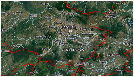
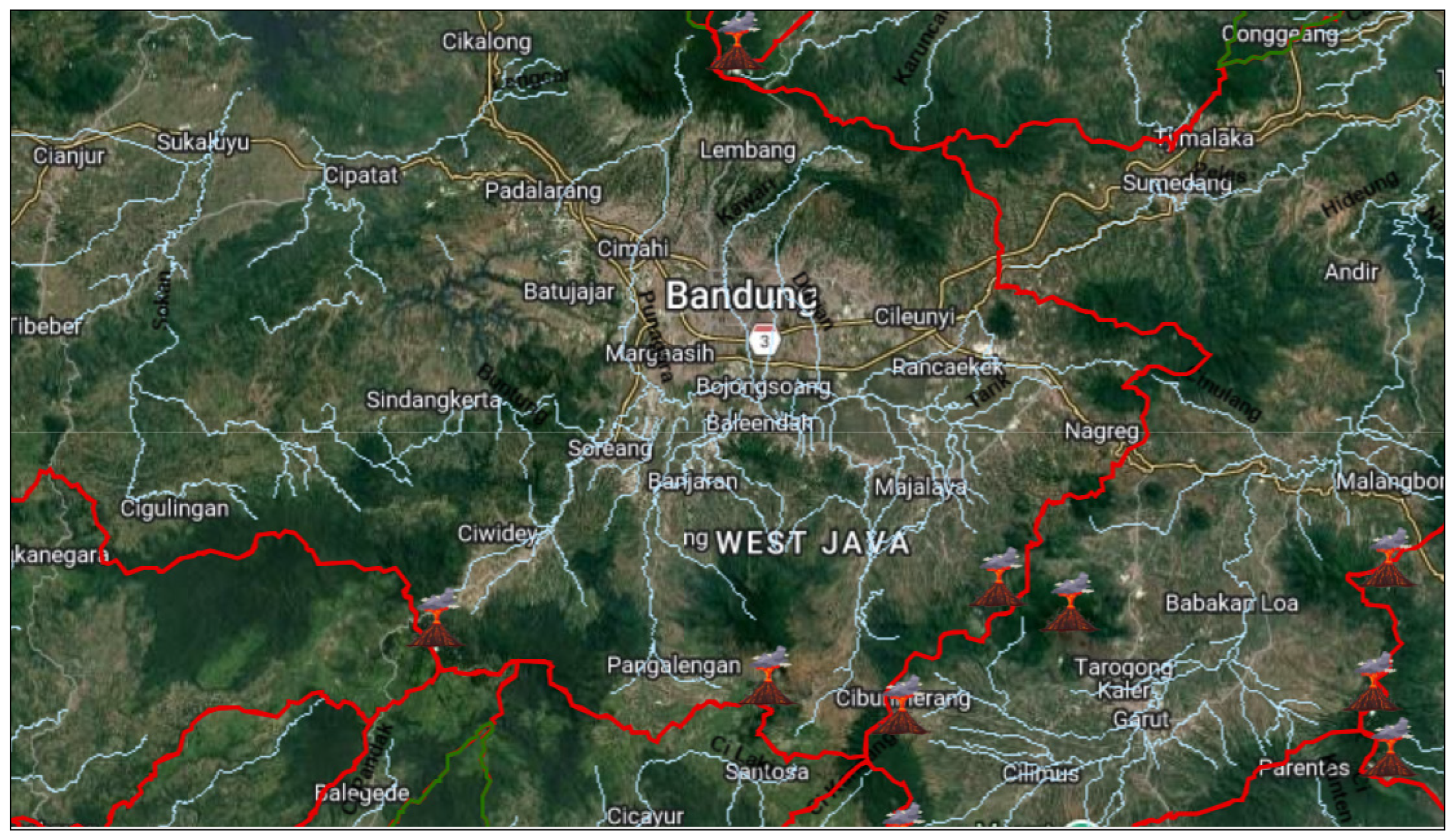
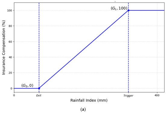
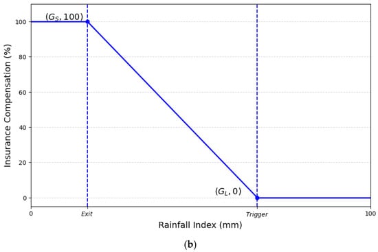
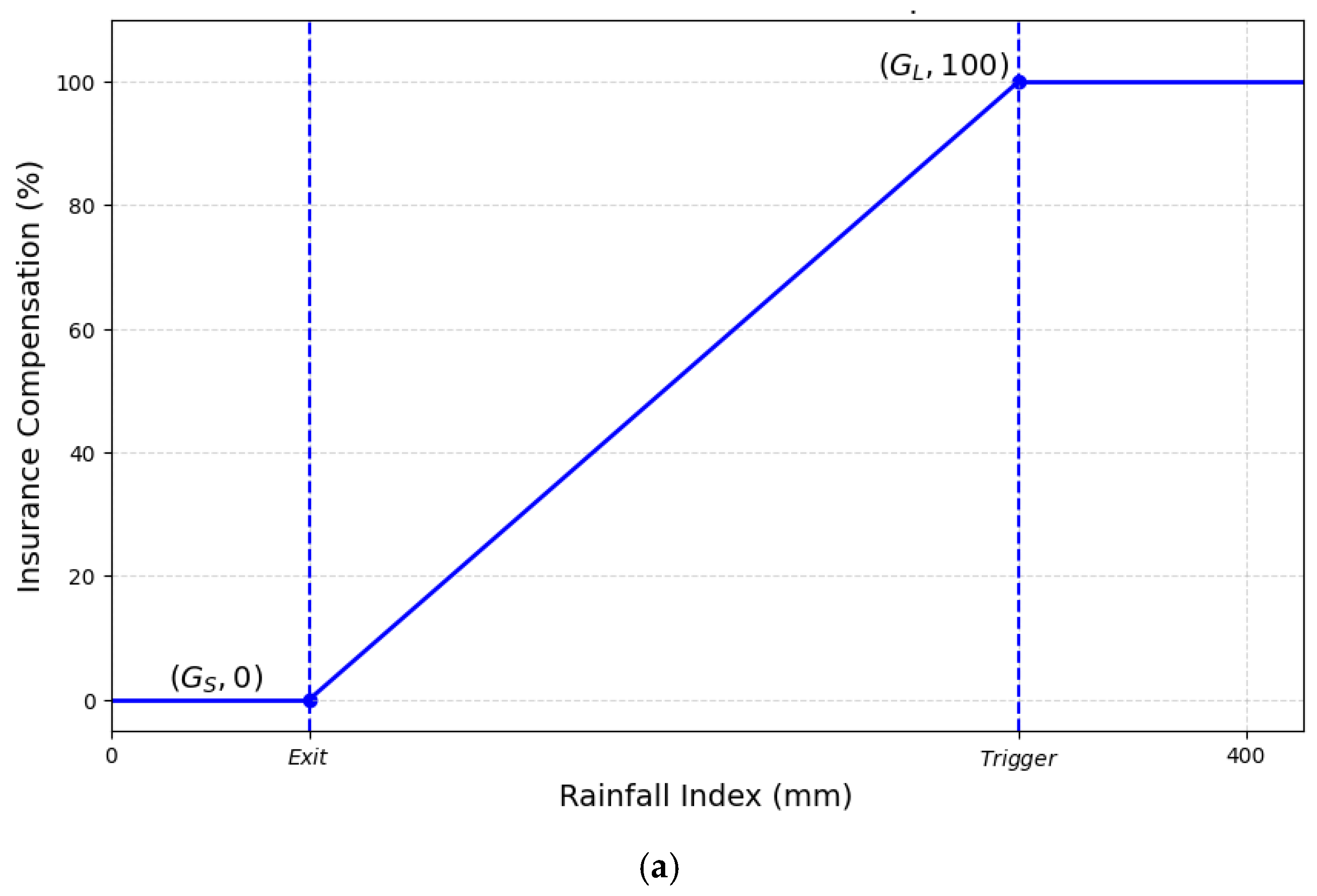
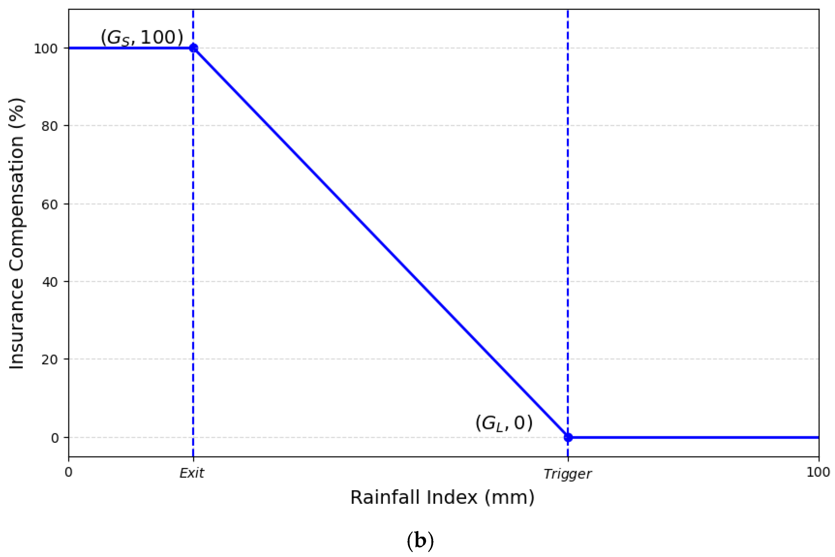
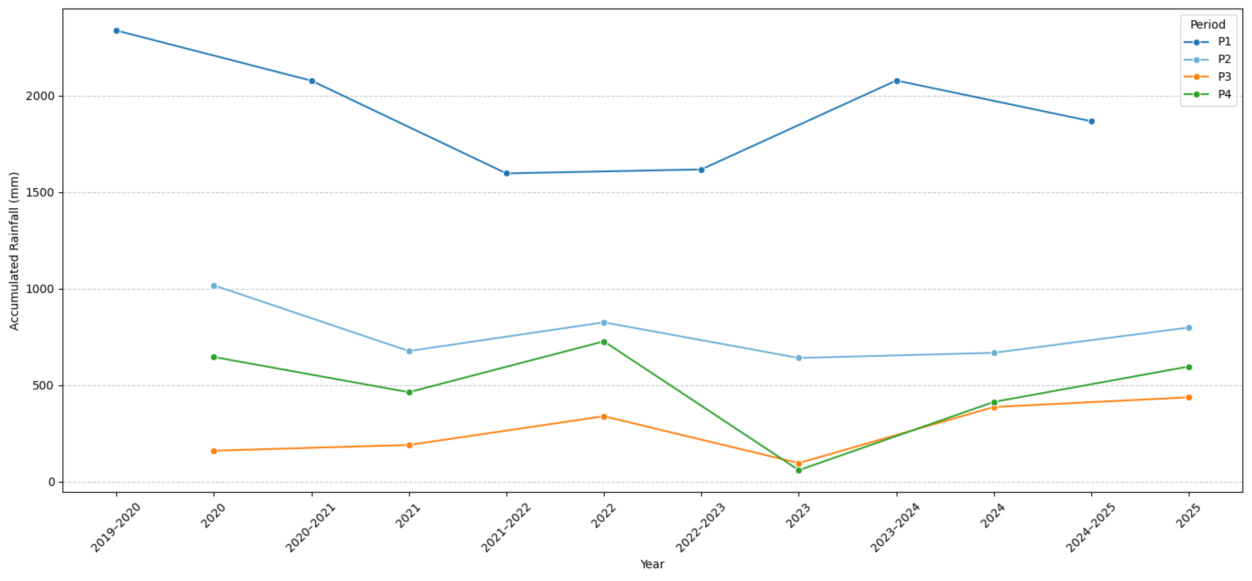
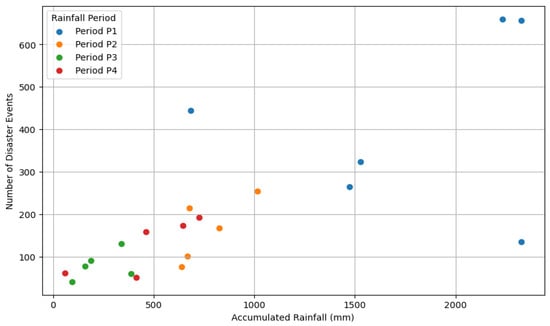
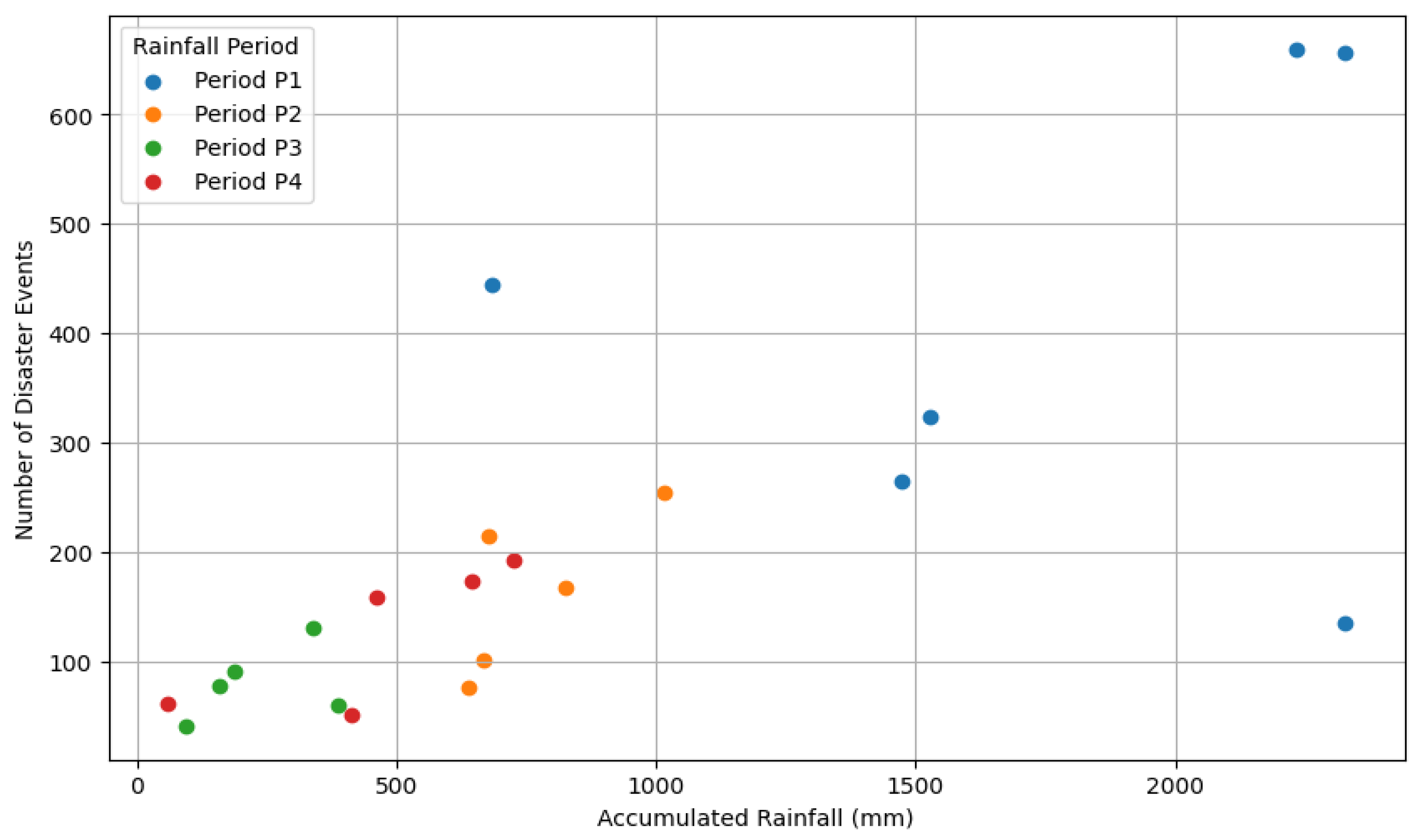
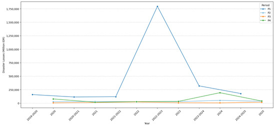
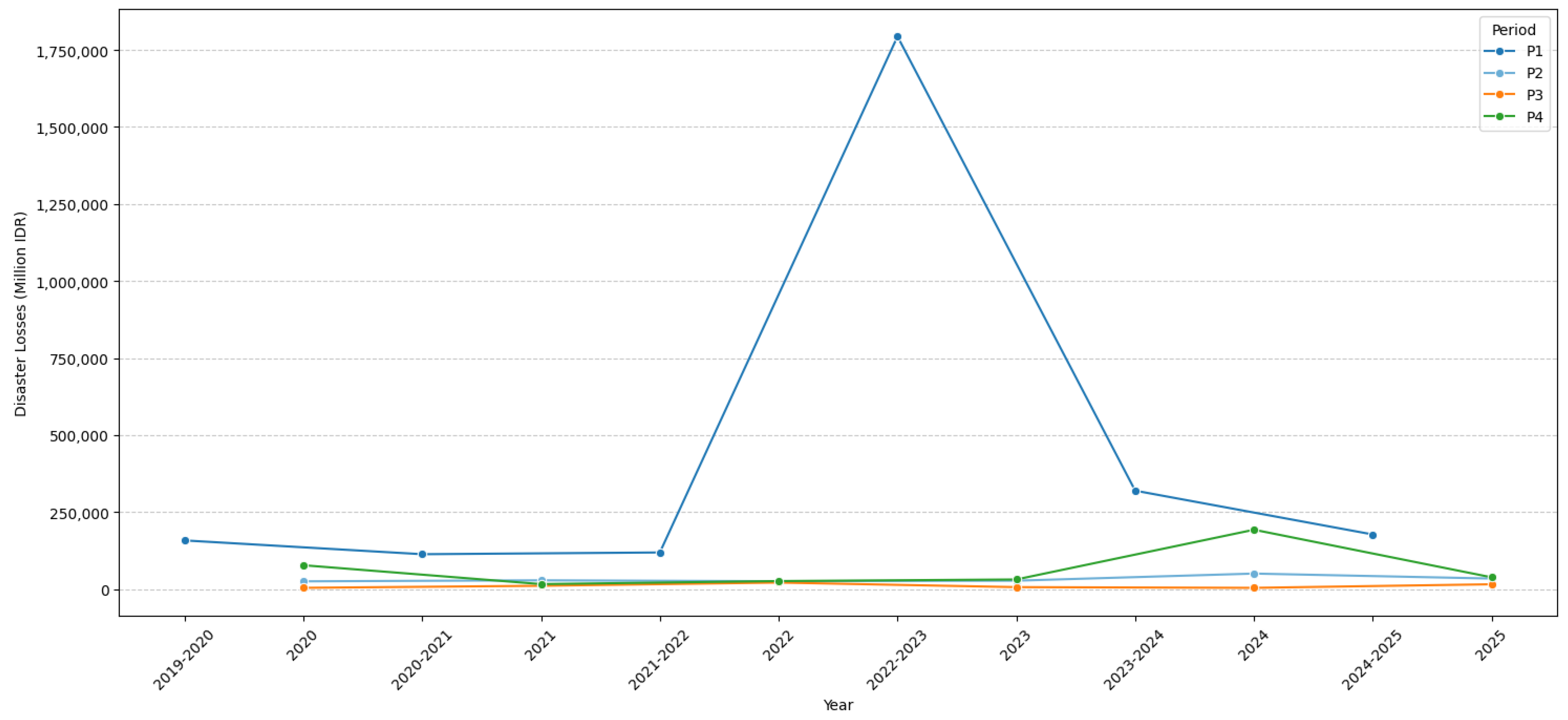
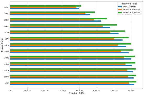
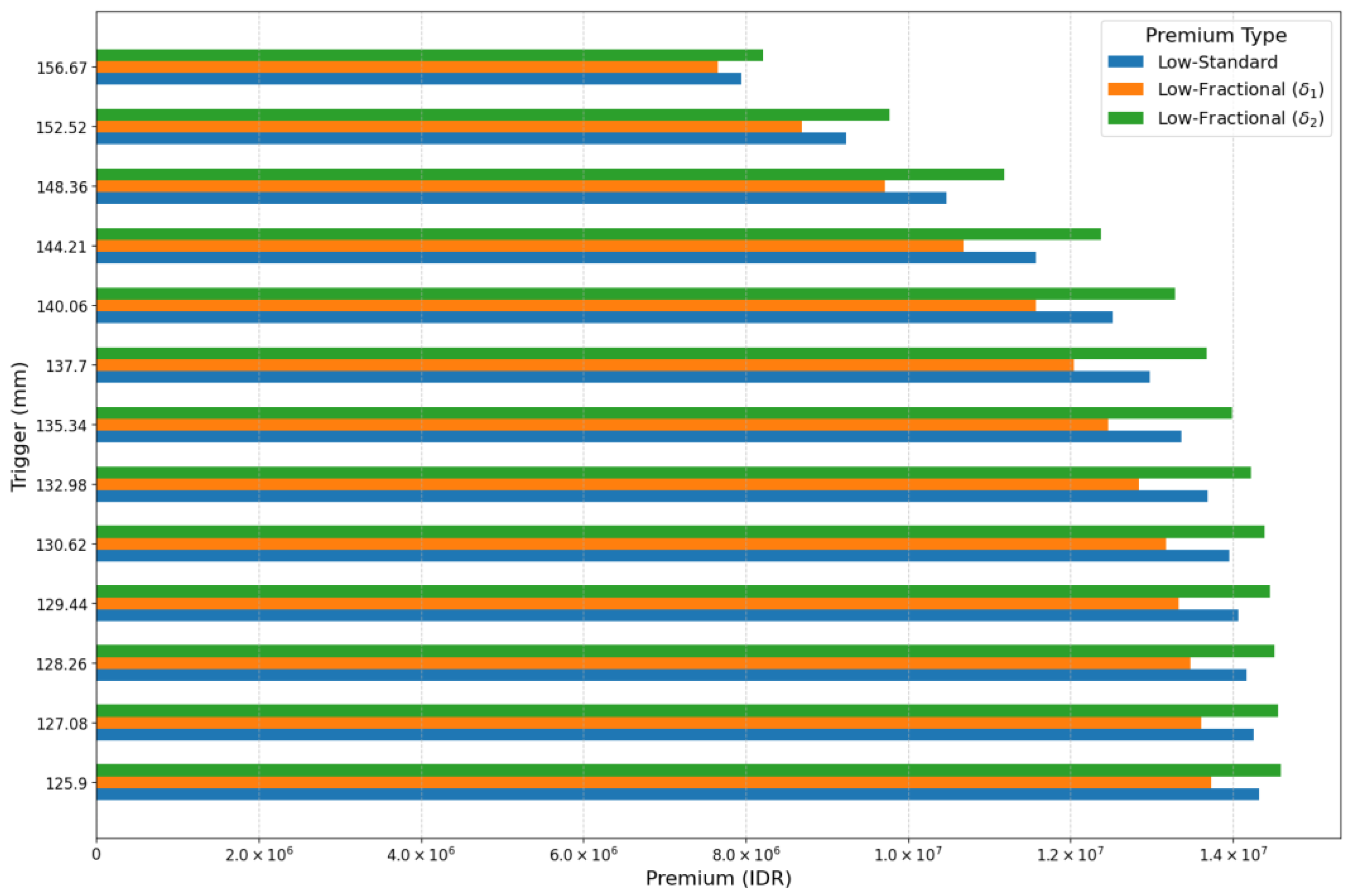
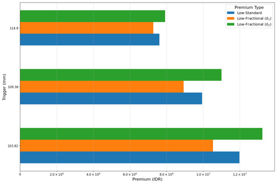
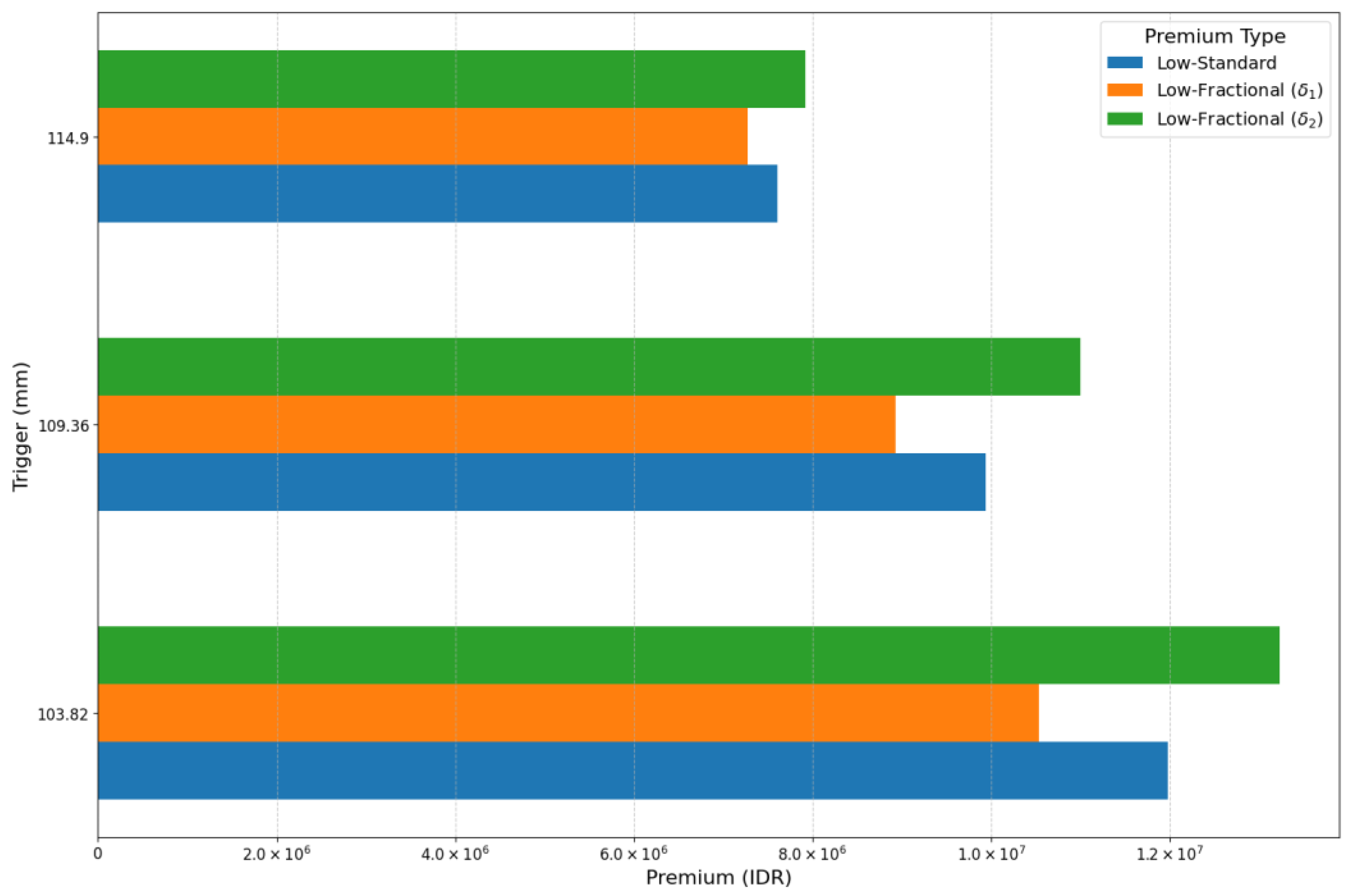
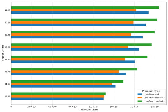
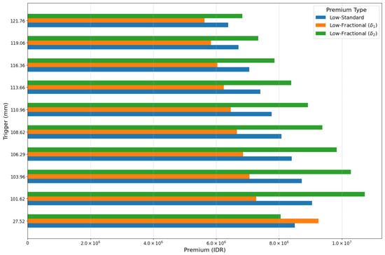

Disclaimer/Publisher’s Note: The statements, opinions and data contained in all publications are solely those of the individual author(s) and contributor(s) and not of MDPI and/or the editor(s). MDPI and/or the editor(s) disclaim responsibility for any injury to people or property resulting from any ideas, methods, instructions or products referred to in the content. |
© 2026 by the authors. Licensee MDPI, Basel, Switzerland. This article is an open access article distributed under the terms and conditions of the Creative Commons Attribution (CC BY) license.