Composite Learning-Based Incremental Neural Control for 2-DOF Helicopter with Adaptive Dynamic Event-Triggering and Input Saturation

Abstract

This study proposes an incremental neural network adaptive control algorithm based on composite learning for a two-degree-of-freedom (2-DOF) helicopter system characterised by dynamic event triggering and input saturation. Firstly, by integrating a composite learning strategy within the incremental neural network control framework, the study aims to overcome the challenges posed by system dynamic uncertainties. The proposed novel update algorithm effectively incorporates estimation error terms into the weight adaptation process, thereby improving the approximation capability for system dynamics while alleviating the dependence on the classical persistent excitation condition. In addition, to reduce the communication load between the controller and the actuator, we introduce an adaptive dynamic event-triggered mechanism. Furthermore, a saturation-resistant auxiliary system is constructed to address the input saturation phenomenon present in the system. Subsequently, the system is proven to be semi-globally consistent and bounded stable via Lyapunov functions. Finally, the effectiveness of the control strategy proposed in this study is verified through simulation.

1. Introduction

Due to their capabilities for vertical takeoff and landing, hovering, and agile maneuvering, helicopters are widely used in logistics, military operations, and emergency response. Two-degree-of-freedom (2-DOF) helicopter systems serve as typical experimental platforms for studying helicopter pitch and yaw motions, effectively reflecting the nonlinear, strongly coupled, and multivariable characteristics of aircraft control. However, this system exhibits characteristics such as multiple inputs and outputs, strong coupling, nonlinearity, and model uncertainty [1]. These factors pose significant challenges for helicopter controller design, and system robustness is particularly critical when high-precision tracking and stable operation are required. Therefore, research on stability control strategies for helicopter systems holds significant value and importance.

Various control methods have been developed for uncertain nonlinear systems to improve tracking accuracy and robustness. For example, in [2], the authors proposed a state-filtered disturbance-rejecting control scheme that abandons the assumption of continuous differentiability of disturbance signals. By employing a state filter for feedforward compensation of both matched and mismatched lumped disturbances, the scheme can adapt to both smooth and non-smooth disturbance scenarios. Furthermore, addressing the trajectory tracking control problem for high-dimensional nonlinear systems, ref. [3] designed a novel multi-layer neural adaptive reinforcement learning algorithm based on the actor-critic framework. However, these methods may rely on relatively precise disturbance reconstruction, additional critic network training, or iterative optimisation processes, which could increase the computational burden and implementation complexity in practical nonlinear control systems. Meanwhile, the 2-DOF helicopter system is a typical nonlinear strongly coupled system with uncertain dynamics, and thus provides a representative platform for evaluating advanced nonlinear control strategies. Regarding the control of helicopter systems, researchers both domestically and internationally have proposed various methods, such as linear quadratic regulators [4], robust control [5], and adaptive control [6]. While these methods have achieved some success in enhancing system stability and improving trajectory tracking performance, most still rely on relatively accurate system models. Consequently, their control performance is easily compromised when faced with complex, unknown nonlinearities, parameter perturbations, and external disturbances. In recent years, neural network (NN) have been widely used in the control of uncertain systems due to their excellent nonlinear approximation capabilities. Among these, radial basis function NN (RBFNN) are frequently employed to estimate unknown uncertainties in helicopter systems because of their simple structure, fast learning speed, and strong local approximation capabilities [7]. For example, to address the control challenges of an unknown 2-DOF helicopter facing unknown hysteresis and output constraints, ref. [8] developed an adaptive NN control algorithm. In [9], the authors proposed a control strategy combining deterministic learning and reinforcement learning for an unknown 2-DOF helicopter system. However, traditional RBFNNs typically employ a fixed network architecture, requiring the number of nodes and the distribution of centers to be determined in advance, making it difficult to balance approximation accuracy and computational efficiency. Furthermore, since the network update law is primarily driven by tracking error, it is prone to insufficient learning information when the error is small. To address these issues, researchers have begun to improve traditional RBFNN control methods in two ways: first, by employing an incremental learning mechanism to enable the network structure to expand online, that is, dynamically adding hidden layer nodes based on changes in system state or approximation error, thereby avoiding the problems of insufficient approximation capability or computational redundancy caused by a fixed network structure [10]; on the other hand, by introducing a composite learning approach, both system tracking error and prediction error information are utilized simultaneously for neural network weight updates, thereby improving parameter estimation accuracy and the ability to learn unknown dynamics [11]. Consequently, the composite learning incremental neural network (CLINN) control method can simultaneously enhance adaptive control performance at both the network structure and parameter update levels, providing a new approach for handling complex, uncertain, and nonlinear systems. In [12], the authors explore a novel control scheme for robotic arms that integrates a CLINN, aiming to address the fixed-time stability problem under input saturation constraints. Current research on CLINN control primarily focuses on general nonlinear systems such as robotic arms; there are few reports on its application to helicopter systems, which provides scope for further expansion in this study.

In addition, with the advancement of embedded controllers and networked control technologies, control signals in 2-DOF helicopter systems typically need to be transmitted between the controller and the actuator via communication networks, and the capacity of these communication channels is limited. Therefore, to improve resource utilization, event-triggered (ET) control methods have gradually been introduced into the control of helicopter systems [13,14]. For example, in [15], the authors proposed continuous-time and ET decentralized output feedback control strategies for interconnected nonlinear systems, and verified their effectiveness and advantages in conserving communication resources through a semi-physical simulation of a 2-DOF helicopter. For unmanned helicopter swarms, ref. [16] introduced an ET federated reinforcement learning framework that achieves efficient and high-precision fault diagnosis while ensuring data privacy and reducing communication costs; its superiority has been validated through semi-physical simulation. In [17], the authors propose an ET adaptive fixed-time control strategy for a 2-DOF helicopter system that integrates reinforcement learning with a disturbance observer, achieving near-optimal, highly robust flight control while reducing communication overhead. Although research on ET control in helicopter systems is well-established, static trigger conditions typically rely on fixed thresholds, making it difficult to simultaneously balance control performance and resource utilization across different operational phases. Therefore, dynamic event-triggered mechanisms enhance flexibility by adjusting trigger thresholds through internal dynamic variables, thereby helping to avoid the Zeno phenomenon [18]. For example, in [19], for a 2-DOF helicopter system, the authors proposed an adaptive bandwidth learning control strategy that combines predefined performance with dynamic event triggering (DET). This approach achieved a higher-precision approximation of system uncertainty and stable trajectory tracking while reducing communication overhead. However, in traditional DET mechanisms, relevant parameters typically require prior setting, and the ability to adjust trigger thresholds is limited, making it difficult to adapt in real time to changes in system errors and operational states. This has inspired us to conduct further research.

In addition to communication constraints, input saturation is another issue that must be addressed in the actual control of helicopters. Due to the physical limitations of the actuators, control inputs are often subject to amplitude constraints; if the control signal exceeds the permissible range, it will result in degraded tracking performance or even compromise system stability. Therefore, it is necessary to further address the issue of input saturation within the event-triggered control framework [20,21]. To date, researchers have developed a variety of algorithms to address the issue of input saturation in helicopter systems. For example, in [22], the authors proposed a multi-approximator-based anti-step adaptive neural fault-tolerant control strategy for a medium-sized unmanned helicopter subject to external disturbances, actuator failures, and input saturation. In [23], for a two-degree-of-freedom helicopter system subject to input saturation and predetermined performance constraints, the authors proposed a fixed-time robust attitude control method that integrates reinforcement learning with a novel sliding mode switching mechanism. Furthermore, for coaxial composite helicopters subject to external disturbances and input saturation, ref. [24] proposes a fixed-time adaptive control algorithm that integrates model-reference adaptive control with sliding mode control. In [25], the authors proposed a neural network control method based on a perturbation observer for a 2-DOF helicopter system with input saturation and output constraints. Although methods for handling input saturation in helicopter systems have achieved satisfactory results, research that simultaneously considers input saturation and adaptive dynamic event-triggered mechanisms within the framework of composite learning incremental neural control remains limited, which provides further scope for exploration in this study.

Inspired by the aforementioned results, this paper proposes a tailored composite learning incremental neural control (CLINC) architecture for a 2-DOF helicopter platform that incorporates an adaptive dynamic event triggering (ADET) mechanism and is subject to input saturation. To effectively address disturbances caused by uncertainties in complex systems, this study introduces the CLINC algorithm; to alleviate communication pressure between the control and execution ends, a corresponding ADET strategy is designed; furthermore, by incorporating an anti-saturation auxiliary system, the phenomenon of actual physical input overload is effectively resolved. Finally, derivations based on Lyapunov stability theory prove that the system state under this control architecture can maintain semi-globally uniform and ultimately bounded (SGUUB) behavior. The key contributions are as follows:

(i)

Unlike [7,8], this study proposes a CLINN approximation framework that can expand network nodes online based on system dynamic information and update weights by combining prediction errors and tracking errors, thereby enhancing the compensation capability for unknown nonlinearities through both network structure adaptation and parameter learning.

(ii)

Unlike [19], this study proposes a new ADET mechanism. By introducing online adjustment parameters, the triggering conditions can be adaptively adjusted in response to changes in system state and tracking error. This ensures that control signals are updated promptly when errors are large, while reducing unnecessary triggering as the system approaches stability.

(iii)

In the presence of both ADET and input saturation, which are mutually coupled, this paper proposes a CLINC strategy. Stability analysis demonstrates that all signals in this closed-loop system are bounded, thereby reducing communication overhead, avoiding the Zeno phenomenon, and mitigating the impact of input saturation on control performance.

2. Problem Statement

2.1. System Function

Based on Lagrange’s equations and the derivation in [19], the nonlinear dynamic model of a 2-DOF helicopter system can be represented by the following system of second-order differential equations:

$$\begin{array}{cc}\hfill \ddot{\varrho }& ={\displaystyle \frac{-mgdcos\varrho -c_{\varrho }\dot{\varrho }-m{d}^2{\dot{\vartheta }}^{2}sin\varrho cos\varrho }{I_{\varrho }+m{d}^2}}+{\displaystyle \frac{k_{11}{u}_1+k_{12}{u}_2}{I_{\varrho }+m{d}^2}}\hfill \end{array}$$

(1)

$$\begin{array}{cc}\hfill \ddot{\vartheta }& ={\displaystyle \frac{-c_{\vartheta }\dot{\vartheta }+2m{d}^2\dot{\vartheta }\dot{\varrho }sin\varrho cos\varrho }{I_{\vartheta }+m{d}^2{cos}^2\varrho }}+{\displaystyle \frac{k_{21}{u}_1+k_{22}{u}_2}{I_{\vartheta }+m{d}^2{cos}^2\varrho }}\hfill \end{array}$$

(2)

where $\varrho$ and $\vartheta$ represent the helicopter’s pitch angle and yaw angle, respectively, i.e., the system’s state variables. $u_1$ and $u_2$ are the drive voltages of the motor. m is the total mass of the system, d indicates the effective length from the rotational pivot to the center of mass, and g is the acceleration due to gravity. $c_{\varrho }$ and $c_{\vartheta }$ are introduced to quantify the viscous friction coefficients acting on the two joints. $I_{\varrho }$ and $I_{\vartheta }$ represent the effective moments of inertia corresponding to their respective rotational axes. $k_{11}$, $k_{12}$, $k_{21}$, and $k_{22}$ denote the thrust torque gain coefficient acting on the system.

Let the system’s total state vector be defined as $x={[x_1^T,x_2^T]}^T$, where $x_1={[\varrho ,\vartheta ]}^T$ and $x_2={[\dot{\varrho },\dot{\vartheta }]}^T$. To facilitate the subsequent design of the controller, we have transformed the dynamic equations into the following standard MIMO form.

$$\begin{array}{cc}\hfill {\dot{x}}_1& =x_2 \hfill \end{array}$$

(3)

$$\begin{array}{cc}\hfill {\dot{x}}_2& =F\left(x\right)+\Delta F\left(x\right)+G\left(x\right)u\hfill \end{array}$$

(4)

where $u={[u_1,u_2]}^T$ denotes the system input, and $\Delta F\left(x\right)$ represents an unknown smooth nonlinear function. Furthermore, $F\left(x\right)$ and $G\left(x\right)$ are defined as:

$$\begin{array}{c}\hfill F\left(x\right)=\left[\begin{array}{c}{\displaystyle \frac{-mgdcos\left(x_{11}\right)-c_{\tau }{x}_{21}-m{d}^2{x}_{22}^{2}sin\left(x_{11}\right)cos\left(x_{11}\right)}{I_{\tau }+m{d}^2}}\\ {\displaystyle \frac{-c_{\vartheta }{x}_{22}+2m{d}^2{x}_{22}{x}_{21}sin\left(x_{11}\right)cos\left(x_{11}\right)}{I_{\vartheta }+m{d}^2{cos}^2\left(x_{11}\right)}}\end{array}\right]\end{array}$$

(5)

$$\begin{array}{c}\hfill G\left(x\right)=\left[\begin{array}{cc}{\displaystyle \frac{k_{11}}{I_{\tau }+m{d}^2}}& {\displaystyle \frac{k_{12}}{I_{\tau }+m{d}^2}}\\ {\displaystyle \frac{k_{21}}{I_{\vartheta }+m{d}^2{cos}^2\left(x_{11}\right)}}& {\displaystyle \frac{k_{22}}{I_{\vartheta }+m{d}^2{cos}^2\left(x_{11}\right)}}\end{array}\right]\end{array}$$

(6)

Given the limited output capacity of the actuators, the actual control input $u\in {\mathbb{R}}^2$ applied to the helicopter system can be defined by the following saturation function. Let $v_i\left(t\right)(i=1,2)$ denote the ideal control variables to be designed; their constrained actual outputs are:

$$\begin{array}{c}\hfill u\left(v_i\right)=\left\{\begin{array}{cc}{U}_{max,i},\hfill & v_i>U_{max,i}\hfill \\ v_i,\hfill & U_{min,i}\le v_i\le U_{max,i}\hfill \\ U_{min,i},\hfill & v_i<U_{min,i}\hfill \end{array}\right.\end{array}$$

(7)

where $U_{max,i}$ and $U_{min,i}$ represent the upper and lower limits of the output for the ith control channel, respectively.

Here, we shall redefine the system controller as

$$\begin{array}{c}\hfill u\left(v\right)=v+\delta \left(v\right)\end{array}$$

(8)

where $v={[v_1,v_2]}^T$ and saturated residual term $\delta \left(v\right)$ is defined as

$$\begin{array}{c}\hfill \delta \left(v_i\right)=\left\{\begin{array}{cc}{U}_{max,i}-v_i,\hfill & v_i>U_{max,i}\hfill \\ 0,\hfill & U_{min,i}\le v_i\le U_{max,i}\hfill \\ U_{min,i}-v_i,\hfill & v_i<U_{min,i}\hfill \end{array}\right.\end{array}$$

(9)

Substituting the above saturated model (8) into the state-space Equation (4), the second-order dynamics of the system can be rewritten as:

$$\begin{array}{cc}\hfill {\dot{x}}_2& =F\left(x\right)+\Delta F\left(x\right)+G\left(x\right)v+G\left(x\right)\delta \left(v\right)\hfill \end{array}$$

(10)

2.2. The Radial Basis Function NN Approximator Based on Incremental Learning

It is well known that RBFNNs are widely favoured for their powerful nonlinear approximation capabilities. In theory, provided there is a sufficient number of nodes in the hidden layer, this network is capable of approximating any continuous nonlinear function to any degree of accuracy. However, in practical applications, due to limitations on the number of nodes, the approximation process inevitably introduces approximation errors.

A nonlinear function $E\left(x\right)$ can be represented by an RBFNN in the following form:

$$\begin{array}{c}\hfill E\left(x\right)={\Theta }^T\varphi \left(x\right)+\omega \left(x\right)\end{array}$$

(11)

where $\Theta \in {\mathbb{R}}^{n\times k}$ represents the weight matrix, $\varphi \left(x\right)\in {\mathbb{R}}^k$ is the regression vector of the network, $\omega \left(x\right)\in {\mathbb{R}}^n$ denotes a bounded approximation error, with $\parallel \omega \left(x\right)\parallel \le \overline{\omega }$, and $x\in {\mathbb{R}}^m$ denotes the input state vector.

Owing to the Gaussian function’s advantages of having a simple form and deriving all orders of derivatives, it is commonly chosen as the radial basis function for RBFNNs. Its expression is as follows [1]:

$$\begin{array}{c}\hfill {\varphi }_i\left(x\right)=exp\left[-{\displaystyle \frac{{(x-c_i)}^T(x-c_i)}{{\rho }_i^2}}\right],i=1,\dots ,k\end{array}$$

(12)

where $c_i\in {\mathbb{R}}^m$ denotes the centre of the ith basis function, and ${\rho }_i\in {\mathbb{R}}^{+}$ corresponds to its standard deviation.

Since traditional RBFNNs often require the positions of nodes to be set manually in advance, this can easily lead to mapping errors due to a lack of prior knowledge. To overcome this limitation, this paper introduces an incremental learning mechanism. During the initialisation phase, the system sets the initial state directly to the first node of the network [12]:

$$\begin{array}{c}\hfill c\left(t_0\right)=x\end{array}$$

(13)

In the subsequent process, the network will evaluate in real time the geometric distance between the current input x and the existing set of nodes c. Within each sampling period T, the set of nodes evolves according to the following logic.

$$\begin{array}{c}\hfill c(t+T)=\left\{\begin{array}{cc}\left[c\left(t\right),c_{\mathrm{new}}\right],\hfill & D>\tau \hfill \\ c\left(t\right),\hfill & D\le \tau \hfill \end{array}\right.\end{array}$$

(14)

where $D=\left|\right|x-c^{\ast }\left|\right|$ denotes the Euclidean distance between the input vector x and the centroid reference point $c^{\ast }$. $\tau$ is the predefined distance threshold. The centre-of-mass reference point $c^{\ast }$ is obtained by calculating the centre of mass of the b nodes closest to the current input.

Finally, the generation rule for the new node $c_{new}$ is defined as follows:

$$\begin{array}{c}\hfill c_{\mathrm{new}}=c^{\ast }+\kappa \left(x-c^{\ast }\right)\end{array}$$

(15)

where $\kappa >0$ is the learning factor that determines the node expansion rate. This incremental mechanism ensures that the coverage area of the neural network is constantly adjusted in real time in accordance with the system’s trajectory, thereby guaranteeing the effective activation of the nodes.

2.3. Preliminaries

Assumption 1

([13]). For the nonlinear function $G\left(x\right)$ of a 2-DOF helicopter system, there exists a positive constant $\overline{G}$ such that the inequality $\parallel G\left(x\right)\parallel \le \overline{G}$ holds for all system states x.

Assumption 2

([26]). The error term $\delta \left(v\right)$ caused by input saturation is bounded, meaning there exists a positive constant $\overline{\delta }$ such that the following condition always holds.

$$\begin{array}{c}\hfill \parallel \delta \left(v\right)\parallel \le \overline{\delta }\end{array}$$

(16)

Lemma 1

([27]). Let the candidate Lyapunov function $V\left(x\right)$ be continuous and positive-definite over its domain. If the function value $V\left(0\right)$ corresponding to the initial state of the system lies within a known finite range, and the time derivative of $V\left(x\right)$ satisfies the following differential inequality:

$$\begin{array}{c}\hfill \dot{V}\left(x\right)\le -\lambda V\left(x\right)+a_1\end{array}$$

(17)

where $\lambda >0$ and $\rho >0$ are both positive scalar constants. It follows that the Lyapunov function $V\left(x\right)$ remains bounded at all times in the time domain.

3. Controller Design and Stability Analysis

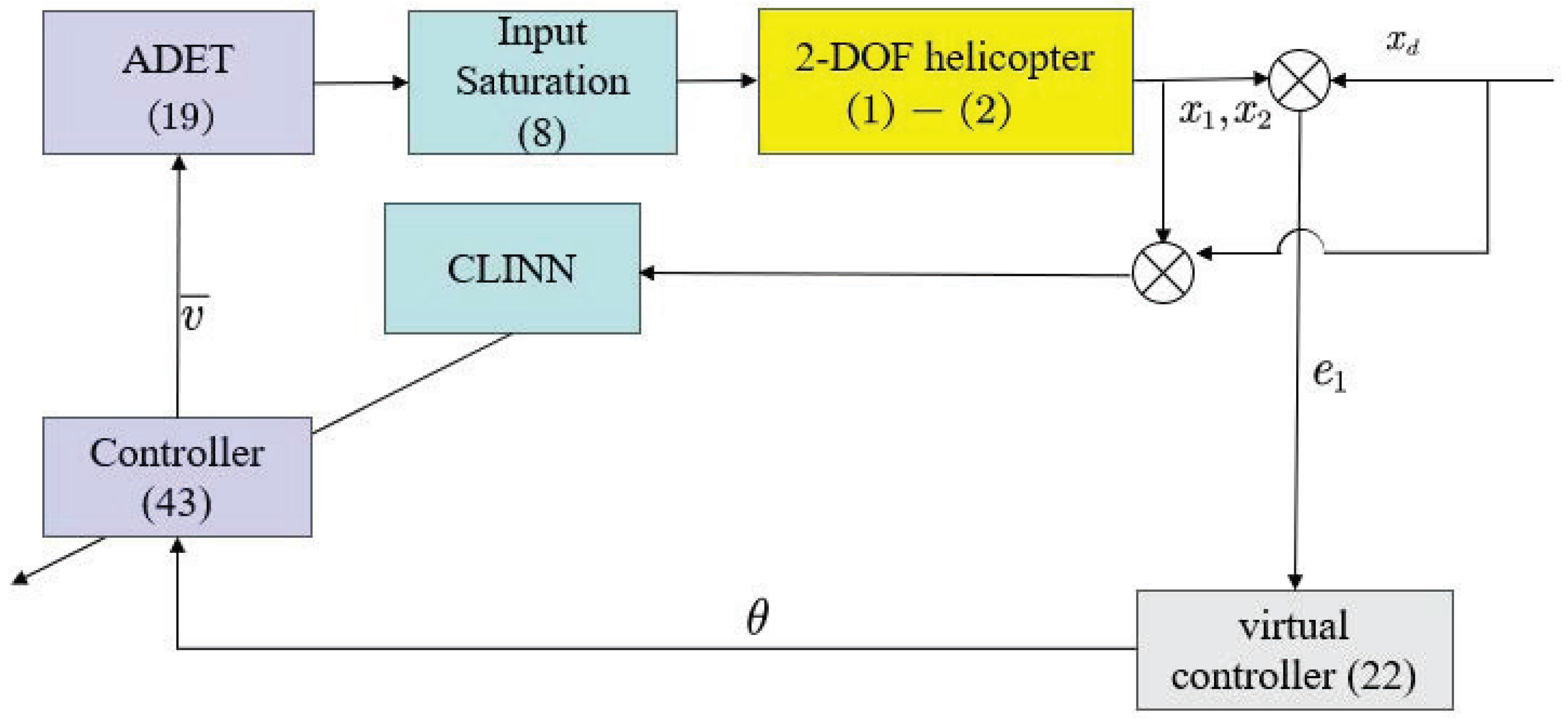
In this section, we first present the controller design for CLINC, then prove the stability of the system, and finally provide a proof to avoid the Zeno phenomenon. The system flowchart is shown in Figure 1.

3.1. Design of CLINN Controller

First, we define the system tracking error as $e_1=x_1-x_d$, where $x_d$ denotes the system reference trajectory.

Furthermore, in the practical application of networked control systems, as the bandwidth resources of physical channels are typically subject to strict constraints, multicast communication between multiple nodes must share limited transmission paths, which often leads to severe channel contention issues. Consequently, exploring and improving the utilisation efficiency of system resources holds profound theoretical value and practical engineering significance. To alleviate communication pressure, non-periodic event-triggered mechanisms have gradually emerged as a research focus.

In this study, to achieve an optimal trade-off between transient control performance and steady-state communication resource conservation, we propose an adaptive dynamic event-triggered scheme. Unlike traditional DET strategies with fixed error weighting parameters, we introduce a time-varying adaptive gain ${\sigma }_{et}\left(t\right)$ driven by the system’s tracking error, defined as:

$${\sigma }_{et}\left(t\right)=\underline{\sigma }+(\overline{\sigma }-\underline{\sigma })exp(-{\gamma }_e\parallel e_1\left(t\right){\parallel }^2)$$

(18)

where $\overline{\sigma }$ and $\underline{\sigma }$ represent the upper and lower bounds of the adaptive parameter, respectively, satisfying $0<\underline{\sigma }\le {\sigma }_{\mathrm{et}}\left(t\right)\le \overline{\sigma }<1$. The positive constant ${\gamma }_e$ is the tuning rate governing the decay speed, and $e_1\left(t\right)$ denotes the system tracking error.

Incorporating this adaptive gain and dynamic auxiliary terms, the control signal hold, trigger condition determination, and evolution of auxiliary variables for this ADET strategy can be expressed by the following mathematical model:

$$\begin{array}{c}\hfill \left\{\begin{array}{c}{v}_i\left(t\right)={\overline{v}}_i\left(s_j\right),\forall t\in [s_j,s_{j+1})\hfill \\ s_{j+1}=inf\left\{t>s_j|{\lambda }_{et}\left(\parallel {\epsilon }_v{\parallel }^2-{\sigma }_{et}\left(t\right){\displaystyle {\sum }_{i=1}^2}{h}_{et,i}{e}_{1i}^2\right)>\varpi \right\}\hfill \\ \dot{\varpi }=-a_{et}\varpi +b_{et}\left({\sigma }_{et}\left(t\right){\displaystyle {\sum }_{i=1}^2}{h}_{et,i}{e}_{1i}^2-{\parallel {\epsilon }_v\parallel }^2\right)\hfill \end{array}\right.\end{array}$$

(19)

where ${\epsilon }_v={[{\epsilon }_{v,1},{\epsilon }_{v,2}]}^T$, and its components ${\epsilon }_{v,i}=v_i-{\overline{v}}_i$ represent the signal deviation caused by the event-triggering strategy. The positive-definite design gains involved in this mechanism include ${\lambda }_{et},h_{et,i}$, and $a_{et}$, as well as the scaling factor $b_{et}\in (0,1]$. The asynchronous update times of the controller are represented by the time series ${\left\{s_j\right\}}_{j=0}^{\infty }$, where the initial value is defined as $s_0=0$. The internal dynamic variable $\varpi \left(t\right)$ is initialized by a strictly positive value, i.e., $\varpi \left(0\right)>0$, which is used to maintain a positive dynamic triggering threshold. From an operational perspective, once the system satisfies the predefined trigger criteria, the current instant is marked as $s_{j+1}$, at which point the control command $v_i$ for the actuator is rapidly synchronised to the latest computed value ${\overline{v}}_i\left(s_{j+1}\right)$. However, during the communication interval $t\in [s_j,s_{j+1})$ between sampling points, constrained by the zero-order hold property, the control input is always latched to the observed value at the previous trigger time, i.e., $v_i\left(t\right)={\overline{v}}_i\left(s_j\right)$. Specifically, during the transient phase when the tracking error $\parallel e_1\left(t\right)\parallel$ is large, ${\sigma }_{et}\left(t\right)$ adaptively shrinks towards its lower bound $\underline{\sigma }$, making the trigger condition easier to breach. This actively increases the communication frequency to guarantee the dynamic performance of the system. Conversely, as the system converges to the steady-state and $\parallel e_1\left(t\right)\parallel$ approaches zero, ${\sigma }_{et}\left(t\right)$ expands towards the upper bound $\overline{\sigma }$, thereby raising the trigger threshold to substantially reduce redundant transmissions and conserve bandwidth.

Next, we define the second error as $e_2=x_2-\theta$, where $\theta$ represents the virtual control signal.

Consider the following Lyapunov candidate function:

$$\begin{array}{c}\hfill V_1={\displaystyle \frac{1}{2}}{e}_1^T{e}_1\end{array}$$

(20)

Taking the derivative of V with respect to time, we obtain

$$\begin{array}{c}\hfill {\dot{V}}_1=e_1^T(e_2+\theta -{\dot{x}}_d)\end{array}$$

(21)

Construct the virtual control signal as follows:

$$\begin{array}{c}\hfill \theta =-K_1{e}_1+{\dot{x}}_d\end{array}$$

(22)

Taking the time derivative of the above virtual control signal, we can get

$$\begin{array}{c}\hfill \dot{\theta }=-K_1{\dot{e}}_1+{\ddot{x}}_d\end{array}$$

(23)

where $K_1\in {\mathbb{R}}^{2\times 2}$ represents the gain coefficient of the virtual controller.

Substituting (22) into (21) yields

$$\begin{array}{c}\hfill {\dot{V}}_1=-e_1^T{K}_1{e}_1+e_1^T{e}_2\end{array}$$

(24)

To compensate for the unknown smooth nonlinear term $\Delta F\left(x\right)$ in the 2-DOF helicopter system, this paper introduces a radial basis function neural network based on incremental learning to approximate it online. The specific expressions are given as follows:

$$\begin{array}{c}\hfill \Delta F\left(x\right)={\Theta }^{\ast T}\varphi \left(x\right)+\omega \left(x\right)\end{array}$$

(25)

where ${\Theta }^{\ast }\in {\mathbb{R}}^{n\times 2}$ represents the ideal weight. $x={[x_1^T,x_2^T]}^T$ represents the state vector of the system. $\omega \left(x\right)\in {\mathbb{R}}^2$ represents the bounded approximation error and satisfies $\parallel \omega \left(x\right)\parallel \le \overline{\omega }$, and $\overline{\omega }$ is a positive constant.

Based on the IRBFNN structure, the online estimation of the unknown term $\Delta F\left(x\right)$ is defined as follows:

$$\begin{array}{c}\hfill \Delta \widehat{F}\left(x\right)={\widehat{\Theta }}^T\varphi \left(x\right)\end{array}$$

(26)

where $\widehat{\Theta }\in {\mathbb{R}}^{n\times 2}$ is the online-updated weight matrix. The weight estimation error is further defined as $\tilde{\Theta }=\widehat{\Theta }-{\Theta }^{\ast }$.

Hence, we can conclude that

$$\begin{array}{c}\hfill \Delta F\left(x\right)={\widehat{\Theta }}^T\varphi \left(x\right)-{\tilde{\Theta }}^T\varphi \left(x\right)+\omega \left(x\right).\end{array}$$

(27)

To further improve the learning accuracy of neural network weights and reduce the dependence on continuous activation conditions, this paper introduces a composite learning mechanism within the IRBFNN framework. The i th component of the unknown vector function $\Delta F\left(x\right)$ is denoted as

$$\begin{array}{c}\hfill \Delta F_i\left(x\right)={\Theta }_i^{\ast T}\varphi \left(x\right)+{\omega }_i\left(x\right),i=1,2\end{array}$$

(28)

where ${\Theta }_i^{\ast }\in {\mathbb{R}}^n$ represents the ideal weight vector corresponding to the ith channel, and ${\omega }_i\left(x\right)$ represents the approximation error of that channel.

Define the historical regression information matrix as

$$\begin{array}{c}\hfill \mathcal{M}\left(t\right)={\int }_0^t{e}^{-{\lambda }_c(t-\tau )}\varphi \left(x\left(\tau \right)\right){\varphi }^T\left(x\left(\tau \right)\right)d\tau \end{array}$$

(29)

Furthermore, the historical target information vector is defined as follows:

$$\begin{array}{c}\hfill {\mathcal{N}}_i\left(t\right)={\int }_0^t{e}^{-{\lambda }_c(t-\tau )}\varphi \left(x\left(\tau \right)\right)\Delta F_i^r\left(\tau \right)d\tau \end{array}$$

(30)

where ${\lambda }_c$ represents the forgetting factor, and $F_i^r\left(\tau \right)$ represents the reconstructable signal of the i th component of the unknown nonlinear term.

Therefore, the composite learning error is defined as

$$\begin{array}{c}\hfill {\mathcal{E}}_i\left(t\right)=\mathcal{M}\left(t\right){\widehat{\Theta }}_i-{\mathcal{N}}_i\left(t\right),i=1,2\end{array}$$

(31)

From (4), we can obtain

$$\begin{array}{c}\hfill \Delta F\left(x\right)={\dot{x}}_2-F\left(x\right)-G\left(x\right)v-G\left(x\right)\delta \left(v\right).\end{array}$$

(32)

Since ${\dot{x}}_2$ is generally not directly measurable, this study introduces a second-order filter to estimate it, the specific expression of which is shown below.

$$\begin{array}{c}\hfill \left\{\begin{array}{c}{\dot{\widehat{x}}}_2=\widehat{a},\hfill \\ \dot{\widehat{a}}={\omega }_c^2(x_2-{\widehat{x}}_2)-2{\zeta }_c{\omega }_c\widehat{a}\hfill \end{array}\right.\end{array}$$

(33)

where ${\widehat{x}}_2$ is the filtered estimate of state $x_2$, $\widehat{a}\in {\mathbb{R}}^2$ is the estimator of ${\dot{x}}_2$, ${\omega }_c>0$ is the filter bandwidth, and ${\zeta }_c>0$ is the damping coefficient. By appropriately selecting ${\omega }_c$ and ${\zeta }_c$, $\widehat{a}$ can be made to approximate ${\dot{x}}_2$ sufficiently in an engineering sense, that is $\widehat{a}\approx {\dot{x}}_2$.

Remark 1.

The second-order filter in (33) is used to generate a feasible estimate of ${\dot{x}}_2$. The selection of its parameters ${\omega }_c$ and ${\zeta }_c$ requires a trade-off between reconstruction accuracy and noise suppression capability. A larger ${\omega }_c$ helps improve the tracking capability of ${\dot{x}}_2$, but increases sensitivity to high-frequency measurement noise; a smaller ${\omega }_c$ is beneficial for noise attenuation, but introduces greater phase lag. The damping coefficient ${\zeta }_c$ primarily affects the transient oscillation characteristics of the estimator; a moderate damping ratio is typically chosen to obtain a smoother estimation response. Provided the parameters are selected appropriately, the reconstruction error introduced by this filter remains bounded and can be incorporated as a bounded perturbation term in subsequent composite learning analyses.

Therefore, the realizable reconfigurable value of an unknown dynamic term is defined as follows:

$$\begin{array}{c}\hfill \Delta F^r\left(x\right)=\widehat{a}-F\left(x\right)-G\left(x\right)v-G\left(x\right)\delta \left(v\right).\end{array}$$

(34)

Let $\Delta F_i^r\left(x\right)$ be the i-th component. This component can then be used as the historical target signal in the composite learning term ${\mathcal{N}}_i\left(t\right)$. Therefore, ${\mathcal{N}}_i\left(t\right)$ is implemented as

$$\begin{array}{c}\hfill {\mathcal{N}}_i\left(t\right)={\int }_0^t{e}^{-{\lambda }_c(t-\tau )}\varphi \left(x\left(\tau \right)\right)\Delta F_i^r\left(\tau \right)d\tau .\end{array}$$

(35)

Furthermore, the reconstruction error is defined.

$$\begin{array}{c}\hfill {\xi }_f\left(x\right)=\Delta F^r\left(x\right)-\Delta F\left(x\right)\end{array}$$

(36)

And denote its i-th component as ${\xi }_{f,i}\left(x\right)$. If the filter parameters are chosen appropriately, then ${\xi }_{f,i}\left(x\right)$ is a bounded signal.

Substituting $\Delta F_i\left(x\right)$ and $\Delta F_i^r\left(x\right)$ into the definition of ${\mathcal{E}}_i\left(t\right)$, we get

$$\begin{array}{cc}\hfill {\mathcal{E}}_i\left(t\right)& =\mathcal{M}\left(t\right){\widehat{\Theta }}_i-{\int }_0^t{e}^{-{\lambda }_c(t-\tau )}\varphi \left(\chi \left(\tau \right)\right)\Delta F_i^r\left(\tau \right)d\tau \hfill \\ \hfill & =\mathcal{M}\left(t\right){\widehat{\Theta }}_i-{\int }_0^t{e}^{-{\lambda }_c(t-\tau )}\varphi \left(\chi \left(\tau \right)\right)\left({\Theta }_i^{\ast T}\varphi \left(\chi \left(\tau \right)\right)+{\epsilon }_{f,i}\left(\chi \left(\tau \right)\right)+{\xi }_{f,i}\left(\tau \right)\right)d\tau \hfill \\ \hfill & =\mathcal{M}\left(t\right)\left({\widehat{\Theta }}_i-{\Theta }_i^{\ast }\right)+{\Omega }_i\left(t\right)\hfill \\ \hfill & =\mathcal{M}\left(t\right){\tilde{\Theta }}_i+{\Omega }_i\left(t\right)\hfill \end{array}$$

(37)

where ${\Omega }_i\left(t\right)=-{\int }_0^t{e}^{-{\lambda }_c(t-\tau )}\varphi \left(x\left(\tau \right)\right)\left({\epsilon }_{f,i}\left(x\left(\tau \right)\right)+{\xi }_{f,i}\left(\tau \right)\right)d\tau$.

Since both ${\epsilon }_{f,i}\left(\chi \right)$ and ${\xi }_{f,i}\left(\tau \right)$ are bounded, and $\varphi \left(\chi \right)$ is bounded, ${\Omega }_i\left(t\right)$ is also a bounded term. This result shows that the composite learning error ${\mathcal{E}}_i\left(t\right)$ can be decomposed into the sum of the parameter error term $\mathcal{M}\left(t\right){\tilde{\Theta }}_i$ and the bounded perturbation term ${\Omega }_i\left(t\right)$, and thus can be used as an additional learning error signal in Lyapunov analysis.

To facilitate real-time implementation, the above integral form can be further rewritten into an equivalent dynamic form.

$$\begin{array}{c}\hfill \dot{\mathcal{M}}\left(t\right)=-{\lambda }_c\mathcal{M}\left(t\right)+\varphi \left(x\right){\varphi }^T\left(x\right)\end{array}$$

(38)

and

$$\begin{array}{c}\hfill {\dot{\mathcal{N}}}_i\left(t\right)=-{\lambda }_c{\mathcal{N}}_i\left(t\right)+\varphi \left(x\right)\Delta F_i^r,i=1,2\end{array}$$

(39)

In this way, it is not necessary to repeatedly calculate the integral from the initial time to the current time at each time step. Instead, the auxiliary variables $\mathcal{M}\left(t\right)$ and ${\mathcal{N}}_i\left(t\right)$ can be updated online, which greatly reduces the implementation complexity.

Therefore, this study selects the following weight update law:

$$\begin{array}{c}\hfill {\dot{\widehat{\Theta }}}_i={\Gamma }_i^{-1}(\varphi \left(x\right)e_{2,i}-k_{\mathcal{E},i}{\mathcal{E}}_i-{\sigma }_{\Theta ,i}{\widehat{\Theta }}_i),i=1,2\end{array}$$

(40)

where ${\Gamma }_i={\Gamma }_i^T>0$ is the learning rate matrix, $k_{\mathcal{E},i}>0$ is the composite learning gain, ${\sigma }_{\Theta ,i}>0$ is the $\sigma$-correction term, and $e_{2,i}$ is the i-th component of the second-step error vector $e_2$.

Next, we substitute (23) and (25) into the time derivative of $e_2$ to obtain

$$\begin{array}{c}\hfill {\dot{e}}_2=F\left(x\right)+{\Theta }^{\ast T}\varphi \left(x\right)+\omega \left(x\right)+G\left(x\right)\overline{v}+G{\epsilon }_v+G\left(x\right)\delta \left(v\right)-\dot{\theta }\end{array}$$

(41)

To eliminate the input saturation problem caused by the aforementioned $\delta \left(v\right)$, we design the following first-order auxiliary system.

$$\begin{array}{c}\hfill \dot{\zeta }=-K_{\zeta }\zeta +\delta \left(v\right)\end{array}$$

(42)

where $\zeta$ represents the auxiliary system state, and $K_{\zeta }\in {\mathbb{R}}^{2\times 2}$ is the positive definite diagonal decay matrix.

Therefore, the CLINN controller designed in this study is as follows:

$$\begin{array}{c}\hfill \overline{v}=G^{-1}(-F\left(x\right)-{\widehat{\Theta }}^T\varphi \left(x\right)-e_1-K_2{e}_2+C_{\zeta }\zeta +\dot{\theta })\end{array}$$

(43)

where $K_2\in {\mathbb{R}}^{2\times 2}$ is the control gain and $C_{\zeta }\in {\mathbb{R}}^{2\times 2}$ is the auxiliary system compensation feedback gain.

3.2. Stability Analysis

Theorem 1.

Considering the input-saturated 2-DOF helicopter system (1) and (2) and the ADET (19), this study designs a CLINN controller (43) and constructs a corresponding CL adaptive update rate (40). The developed control strategy ensures that the system is SGUUB, and prevents the occurrence of the Zeno phenomenon, which also implies that the time interval between events has a strictly positive lower bound.

Proof. 

First, let us consider the second Lyapunov candidate function as

$$\begin{array}{c}\hfill V_2=V_1+{\displaystyle \frac{1}{2}}{e}_2^T{e}_2+{\displaystyle \frac{1}{2}}{\displaystyle \sum _{i=1}^2}{\tilde{\Theta }}_i^T{\Gamma }_i{\tilde{\Theta }}_i+{\displaystyle \frac{1}{2}}{\zeta }^T\zeta \end{array}$$

(44)

To incorporate the internal dynamic variables in the ADET mechanism into the stability analysis, the following augmented Lyapunov function is further introduced:

$$\begin{array}{c}\hfill V_3=V_2+{\rho }_{\varpi }\varpi \end{array}$$

(45)

where ${\rho }_{\varpi }>0$. Since $\varpi \left(0\right)>0$ and $\varpi \left(t\right)\ge 0$ under the proposed ADET mechanism, ${\rho }_{\varpi }\varpi$ is a non-negative term.

Substituting(19), (24) and (41)–(43) into the time derivative of $V_3$ yields

$$\begin{array}{cc}\hfill {\dot{V}}_3& =-e_1^T{K}_1{e}_1+e_1^T{e}_2+e_2^T(F\left(x\right)+{\Theta }^{\ast T}\varphi \left(x\right)+\omega \left(x\right)-F\left(x\right)-{\widehat{\Theta }}^T\varphi \left(x\right)-e_1-K_2{e}_2\hfill \\ & +C_{\zeta }\zeta +\dot{\theta }-\dot{\theta })+G\left(x\right){\epsilon }_v+{\displaystyle \sum _{i=1}^2}{\tilde{\Theta }}_i^T\left(\varphi \left(x\right)e_{2,i}-k_{\mathcal{E},i}{\mathcal{E}}_i-{\sigma }_{\Theta ,i}{\widehat{\Theta }}_i\right)+{\zeta }^T(-K_{\zeta }\zeta +\delta \left(v\right))\hfill \\ \hfill & +e_2^{T}G\left(x\right)\delta \left(v\right)+{\rho }_{\varpi }(-a_{et}\varpi +b_{et}({\sigma }_{et}\left(t\right){\displaystyle \sum _{i=1}^2}{h}_{et,i}{e}_{1i}^2-\parallel {\epsilon }_v{\parallel }^2))\hfill \\ \hfill & =-e_1^T{K}_1{e}_1+e_2^T{\Theta }^{\ast T}\varphi \left(x\right)+e_2^T\omega \left(x\right)-e_2^T{\widehat{\Theta }}^T\varphi \left(x\right)-e_2^T{K}_2{e}_2+e_2^T{C}_{\zeta }\zeta +e_2^{T}G\left(x\right){\epsilon }_v\hfill \\ & +{\displaystyle \sum _{i=1}^2}{\tilde{\Theta }}_i^T\varphi \left(x\right)e_{2,i}-{\displaystyle \sum _{i=1}^2}{\tilde{\Theta }}_i^T{k}_{\mathcal{E},i}{\mathcal{E}}_i-{\displaystyle \sum _{i=1}^2}{\sigma }_{\Theta ,i}{\tilde{\Theta }}_i^T{\widehat{\Theta }}_i-{\zeta }^T{K}_{\zeta }\zeta +{\zeta }^T\delta \left(v\right)-a_{et}{\rho }_{\varpi }\varpi \hfill \\ & +e_2^{T}G\left(x\right)\delta \left(v\right)+{\rho }_{\varpi }{b}_{et}{\sigma }_{et}\left(t\right){\displaystyle \sum _{i=1}^2}{h}_{et,i}{e}_{1i}^2-{\rho }_{\varpi }{b}_{et}{\parallel {\epsilon }_v\parallel }^2\hfill \\ \hfill & =-e_1^T{K}_1{e}_1+e_2^T\omega \left(x\right)-e_2^T{K}_2{e}_2+e_2^T{C}_{\zeta }\zeta +e_2^{T}G\left(x\right){\epsilon }_v-{\displaystyle \sum _{i=1}^2}{\tilde{\Theta }}_i^T{k}_{\mathcal{E},i}{\mathcal{E}}_i-{\displaystyle \sum _{i=1}^2}{\sigma }_{\Theta ,i}{\tilde{\Theta }}_i^T{\widehat{\Theta }}_i\hfill \\ & -{\zeta }^T{K}_{\zeta }\zeta +{\zeta }^T\delta \left(v\right)+e_2^{T}G\left(x\right)\delta \left(v\right)-a_{et}{\rho }_{\varpi }\varpi +{\rho }_{\varpi }{b}_{et}{\sigma }_{et}\left(t\right){\displaystyle \sum _{i=1}^2}{h}_{et,i}{e}_{1i}^2-{\rho }_{\varpi }{b}_{et}{\parallel {\epsilon }_v\parallel }^2\hfill \end{array}$$

(46)

Let $Q\left(t\right)={\sigma }_{et}\left(t\right){\sum }_{i=1}^2{h}_{et,i}{e}_{1i}^2$. Since $0<\underline{\sigma }\le {\sigma }_{\mathrm{et}}\left(t\right)\le \overline{\sigma }<1$ and $h_{et,i}>0$, it follows that

$$\begin{array}{c}\hfill 0\le q\left(t\right)\le \overline{\sigma }\overline{h}{\parallel e_1\parallel }^2\end{array}$$

(47)

where $\overline{h}=max\left\{h_{\mathrm{et},1},h_{\mathrm{et},2}\right\}$. From (37), we obtain

$$\begin{array}{c}\hfill -{\displaystyle \sum _{i=1}^2}{\tilde{\Theta }}_i^T{k}_{\mathcal{E},i}{\mathcal{E}}_i=-{\displaystyle \sum _{i=1}^2}{k}_{\mathcal{E},i}{\tilde{\Theta }}_i^T\mathcal{M}\left(t\right){\tilde{\Theta }}_i-{\displaystyle \sum _{i=1}^2}{k}_{\mathcal{E},i}{\tilde{\Theta }}_i^T{\Omega }_i\left(t\right)\end{array}$$

(48)

By Yang’s inequality yields

$$e_2^T\omega \left(x\right)\le {\displaystyle \frac{1}{2}}{e}_2^T{e}_2+{\displaystyle \frac{1}{2}}{\overline{\omega }}^2$$

(49)

$$e_2^T{C}_{\zeta }\zeta \le {\displaystyle \frac{1}{2}}{e}_2^T{e}_2+{\displaystyle \frac{1}{2}}{\parallel C_{\zeta }\parallel }^2{\zeta }^T\zeta$$

(50)

$$e_2^{T}G\left(x\right){\epsilon }_v\le {\displaystyle \frac{1}{2}}{e}_2^T{e}_2+{\displaystyle \frac{{\overline{G}}^2}{2}}{\parallel {\epsilon }_v\parallel }^2$$

(51)

$$e_2^{T}G\left(x\right)\delta \left(v\right)\le {\displaystyle \frac{1}{2}}{e}_2^T{e}_2+{\displaystyle \frac{1}{2}}{\overline{G}}^2{\overline{\delta }}^2$$

(52)

$${\zeta }^T\delta \left(v\right)\le {\displaystyle \frac{1}{2}}{e}_2^T{e}_2+{\displaystyle \frac{1}{2}}{\overline{\delta }}^2$$

(53)

$$-{\sigma }_{\Theta ,i}{\tilde{\Theta }}_i^T{\widehat{\Theta }}_i\le -{\displaystyle \frac{{\sigma }_{\Theta ,i}}{2}}\parallel {\tilde{\Theta }}_i{\parallel }^2+{\displaystyle \frac{{\sigma }_{\Theta ,i}}{2}}{\parallel {\Theta }_i^{\ast }\parallel }^2$$

(54)

$$-k_{\mathcal{E},i}{\tilde{\Theta }}_i^T{\Omega }_i\left(t\right)\le {\displaystyle \frac{k_{\mathcal{E},i}}{2}}\parallel {\tilde{\Theta }}_i{\parallel }^2+{\displaystyle \frac{k_{\mathcal{E},i}}{2}}{\parallel {\Omega }_i\left(t\right)\parallel }^2$$

(55)

Since the historical information matrix $\mathcal{M}\left(t\right)$ in composite learning is positive semi-definite, we obtain $\mathcal{M}\left(t\right)\ge 0$:

$$\begin{array}{c}\hfill -k_{\mathcal{E},i}{\tilde{\Theta }}_i^T\mathcal{M}\left(t\right){\tilde{\Theta }}_i\le 0\end{array}$$

(56)

Substituting (49)–(55) into (46), we have

$$\begin{array}{cc}\hfill {\dot{V}}_3& \le -(K_1-{\rho }_{\varpi }{b}_{et}\overline{\sigma }\overline{h})e^T{e}_1-\left(K_2-{\displaystyle \frac{1}{2}}{\parallel C_{\zeta }\parallel }^2-{\displaystyle \frac{1}{2}}-{\displaystyle \frac{1}{2}}{\overline{G}}^2\right)e_2^T{e}_2\hfill \\ \hfill & -{\displaystyle \sum _{i=1}^2}\left({\displaystyle \frac{{\sigma }_{\Theta ,i}}{2}}-{\displaystyle \frac{k_{\mathcal{E},i}}{2}}\right){\parallel {\tilde{\Theta }}_i\parallel }^2-\left(K_{\zeta }-1\right){\zeta }^T\zeta -a_{et}{\rho }_{\varpi }\varpi \hfill \\ \hfill & +{\displaystyle \frac{1}{2}}{\overline{\omega }}^2+({\displaystyle \frac{1}{2}}+{\displaystyle \frac{{\overline{G}}^2}{2}}){\overline{\delta }}^2+{\displaystyle \sum _{i=1}^2}\left({\displaystyle \frac{{\sigma }_{\Theta ,i}}{2}}\parallel {\Theta }_i^{\ast }{\parallel }^2+{\displaystyle \frac{k_{\mathcal{E},i}}{2}}{\parallel {\Omega }_i\left(t\right)\parallel }^2\right)+({\displaystyle \frac{{\overline{G}}^2}{2}}-{\rho }_{\varpi }{b}_{et}){\parallel {\epsilon }_v\parallel }^2\hfill \\ \hfill & \le -c_{0}V+B_0\hfill \end{array}$$

(57)

where

$$\begin{array}{cc}\hfill c_0=& min\{2{\lambda }_{min}(K_1-\left({\rho }_{\varpi }{b}_{et}\overline{\sigma }\overline{h}\right)I),2{\lambda }_{min}(K_2-({\displaystyle \frac{1}{2}}\parallel C_{\zeta }{\parallel }^2+{\displaystyle \frac{1}{2}}+{\displaystyle \frac{1}{2}}{\overline{G}}^2\left)I\right),2{\lambda }_{min}(K_{\zeta }-I),\hfill \\ & \underset{i=1,2}{min}{\displaystyle \frac{2\left(\frac{{\sigma }_{\Theta ,i}}{2}-\frac{k_{\mathcal{E},i}}{2}\right)}{{\lambda }_{max}\left({\Gamma }_i\right)}},a_{et}\}\hfill \end{array}$$

(58)

and

$$\begin{array}{c}\hfill {\displaystyle \frac{1}{2}}{\overline{\omega }}^2+({\displaystyle \frac{1}{2}}+{\displaystyle \frac{{\overline{G}}^2}{2}}){\overline{\delta }}^2+{\displaystyle \sum _{i=1}^2}\left({\displaystyle \frac{{\sigma }_{\Theta ,i}}{2}}\parallel {\Theta }_i^{\ast }{\parallel }^2+{\displaystyle \frac{k_{\mathcal{E},i}}{2}}{\parallel {\Omega }_i\left(t\right)\parallel }^2\right)+({\displaystyle \frac{{\overline{G}}^2}{2}}-{\rho }_{\varpi }{b}_{et}){\parallel \epsilon \parallel }^2\end{array}$$

(59)

To ensure the stability of the closed-loop system, all relevant parameters in the controller design must satisfy the following conditions:

$$\begin{array}{c}\hfill {\lambda }_{min}(K_1-({\rho }_{\varpi }{b}_{et}\overline{\sigma }\overline{h})I)>0,{\lambda }_{min}(K_2-({\displaystyle \frac{1}{2}}\parallel C_{\zeta }{\parallel }^2+{\displaystyle \frac{1}{2}}+{\displaystyle \frac{1}{2}}{\overline{G}}^2)I)>0\end{array}$$

(60)

$$\begin{array}{c}\hfill {\lambda }_{min}(K_{\zeta }-I)>0,\underset{i=1,2}{min}{\displaystyle \frac{2\left(\frac{{\sigma }_{\Theta ,i}}{2}-\frac{k_{\mathcal{E},i}}{2}\right)}{{\lambda }_{max}\left({\Gamma }_i\right)}}>0\end{array}$$

(61)

Based on (57), we can conclude that

$$\begin{array}{c}\hfill 0\le V_2\left(t\right)\le {\displaystyle \frac{B_0}{c_0}}+\left[V_2\left(0\right)-{\displaystyle \frac{B_0}{c_0}}\right]e^{-c_{0}t}\end{array}$$

(62)

First, from (62), we obtain the limit ${lim}_{t\to \infty }{V}_2\left(t\right)={\displaystyle \frac{B_0}{c_0}}$, which mathematically proves that the Lyapunov function $V_2$ is bounded. Second, based on the key implication that $V_2$ is bounded, it can be inferred that the tracking errors $e_1$ and $e_2$ in the system, the auxiliary system state $\zeta$, and the IRBFNN weight estimation error $\tilde{\Theta }$ are all bounded. Since the reference system state $x_d$ is bounded, it follows that the actual state $x_1$ remains bounded. Consequently, the virtual control law $\theta$ and the actual continuous control law v are also bounded. This ensures that all signals in the closed-loop system satisfy the SGUUB conditions.

In addition, the continuous control law $\overline{v}\left(t\right)$ is composed of smooth functions of the bounded closed-loop signals. Hence, on any finite time interval $[0,T]$, $\overline{v}\left(t\right)$ is locally Lipschitz continuous. Therefore, there exists a positive constant ${\kappa }_T$ such that $\parallel \dot{\overline{v}}\left(t\right)\parallel \le {\kappa }_T,t\in [0,T]$. This property will be used in the following Zeno-exclusion analysis. Next, we prove that the proposed ADET mechanism excludes Zeno behavior. For notational simplicity, define

$$q\left(t\right)={\sigma }_{et}\left(t\right){\displaystyle \sum _{i=1}^2}{h}_{et,i}{e}_{1i}^2\left(t\right).$$

(63)

According to the definition of ${\sigma }_{et}\left(t\right)$, it follows that

$$0<\sigma \le {\sigma }_{et}\left(t\right)\le \overline{\sigma }<1.$$

(64)

Since $h_{et,i}>0$, one has

$$q\left(t\right)\ge 0.$$

(65)

For $t\in [s_j,s_{j+1})$, the event-triggering condition is not violated. Therefore,

$${\lambda }_{et}\left(\parallel {\epsilon }_v{\left(t\right)\parallel }^2-q\left(t\right)\right)\le \varpi \left(t\right).$$

(66)

It follows that

$$q\left(t\right)-\parallel {\epsilon }_v{\left(t\right)\parallel }^2\ge -{\displaystyle \frac{\varpi \left(t\right)}{{\lambda }_{et}}}.$$

(67)

Substituting the above inequality into the dynamic equation of $\varpi \left(t\right)$ gives

$$\begin{array}{cc}\hfill \dot{\varpi }\left(t\right)& =-a_{et}\varpi \left(t\right)+b_{et}\left(q\left(t\right)-\parallel {\epsilon }_v{\left(t\right)\parallel }^2\right)\hfill \\ & \ge -\left(a_{et}+{\displaystyle \frac{b_{et}}{{\lambda }_{et}}}\right)\varpi \left(t\right).\hfill \end{array}$$

(68)

Let

$${\alpha }_{\varpi }=a_{et}+{\displaystyle \frac{b_{et}}{{\lambda }_{et}}}.$$

(69)

By the comparison principle, if $\varpi \left(0\right)>0$, then for any finite time interval $[0,T]$,

$$\varpi \left(t\right)\ge \varpi \left(0\right)e^{-{\alpha }_{\varpi }t}\ge \varpi \left(0\right)e^{-{\alpha }_{\varpi }T}>0,t\in [0,T].$$

(70)

Hence, the internal dynamic variable $\varpi \left(t\right)$ remains strictly positive over any finite time interval.

At each triggering instant $s_j$, the held input is updated by

$$v\left(t\right)=\overline{v}\left(s_j\right),t\in [s_j,s_{j+1}),$$

(71)

and thus the event-triggering error satisfies

$${\epsilon }_v\left(s_j\right)=v\left(s_j\right)-\overline{v}\left(s_j\right)=0.$$

(72)

For $t\in [s_j,s_{j+1})$, one has

$${\epsilon }_v\left(t\right)=v\left(t\right)-\overline{v}\left(t\right)=\overline{v}\left(s_j\right)-\overline{v}\left(t\right).$$

(73)

Since $\parallel \dot{\overline{v}}\left(t\right)\parallel \le {\kappa }_T$ on any finite interval $[0,T]$, it follows that

$$\begin{array}{ccc}\hfill \parallel {\epsilon }_v\left(t\right)\parallel & =& \parallel \overline{v}\left(s_j\right)-\overline{v}\left(t\right)\parallel \hfill \\ & \le & {\int }_{s_j}^t\parallel \dot{\overline{v}}\left(\tau \right)\parallel d\tau \hfill \\ & \le & {\kappa }_T(t-s_j).\hfill \end{array}$$

(74)

At the next triggering instant $s_{j+1}$, by the definition of the triggering rule and the continuity of the involved signals, one has

$${\lambda }_{et}\left(\parallel {\epsilon }_v\left(s_{j+1}\right){\parallel }^2-q\left(s_{j+1}\right)\right)\ge \varpi \left(s_{j+1}\right).$$

(75)

Therefore,

$$\begin{array}{cc}\hfill \parallel {\epsilon }_v\left(s_{j+1}\right){\parallel }^2& \ge q\left(s_{j+1}\right)+{\displaystyle \frac{\varpi \left(s_{j+1}\right)}{{\lambda }_{et}}}\hfill \\ & \ge {\displaystyle \frac{\varpi \left(s_{j+1}\right)}{{\lambda }_{et}}}.\hfill \end{array}$$

(76)

Using the lower bound of $\varpi \left(t\right)$ on $[0,T]$, we further obtain

$$\parallel {\epsilon }_v\left(s_{j+1}\right)\parallel \ge \sqrt{{\displaystyle \frac{\varpi \left(0\right)e^{-{\alpha }_{\varpi }T}}{{\lambda }_{et}}}}.$$

(77)

Combining this inequality with

$$\parallel {\epsilon }_v\left(s_{j+1}\right)\parallel \le {\kappa }_T(s_{j+1}-s_j),$$

(78)

yields

$$s_{j+1}-s_j\ge {\displaystyle \frac{1}{{\kappa }_T}}\sqrt{{\displaystyle \frac{\varpi \left(0\right)e^{-{\alpha }_{\varpi }T}}{{\lambda }_{et}}}}\triangleq {\tau }_T>0.$$

(79)

Thus, for any finite time interval $[0,T]$, the inter-event time admits a strictly positive lower bound ${\tau }_T$. Consequently, infinitely many triggering instants cannot occur within a finite time interval, and the Zeno behavior is excluded. □

Remark 2.

In the ADET mechanism, the various tuning parameters have different effects on the trigger frequency and tracking performance. The parameter ${\lambda }_{et}$ primarily determines the sensitivity of the event trigger condition; appropriately increasing ${\lambda }_{et}$ makes it easier to satisfy the trigger condition, thereby increasing the frequency of control signal updates and improving transient response, but the communication overhead also increases accordingly. The parameter $a_{et}$ influences the decay rate of the internal dynamic variable $\varpi \left(t\right)$; a larger $a_{et}$ accelerates the decline of the dynamic threshold, making the system more prone to triggering; conversely, a smaller $a_{et}$ helps reduce the number of triggers but may slow down the transient response. The parameter $b_{et}$ is used to regulate the feedback interaction between the tracking error term and the trigger error; an excessively large value may cause the trigger threshold to change too rapidly, so a small positive value is typically selected to ensure a smooth triggering process. As for the weighting parameter $h_{et,i}$, its function is to adjust the proportion of the tracking error of the ith channel in the trigger threshold. Appropriately increasing $h_{et,i}$ can enhance the influence of that channel’s error on the trigger threshold, helping to reduce redundant triggers during the steady-state phase; however, if the value is too large, it may reduce necessary control updates. The adaptive parameter ${\sigma }_{et}\left(t\right)$ is jointly determined by σ, $\overline{\sigma }$ and ${\gamma }_e$. Specifically, a smaller σ enhances trigger sensitivity during the transient phase, a larger $\overline{\sigma }$ helps reduce unnecessary triggers when the error is small, and ${\gamma }_e$ determines the rate at which ${\sigma }_{et}\left(t\right)$ adjusts in response to changes in the tracking error. Finally, $\varpi \left(0\right)$ primarily influences the dynamic trigger threshold during the initial phase; a larger $\varpi \left(0\right)$ reduces the number of initial triggers, but an excessively large value may affect the timeliness of early control updates. Therefore, the parameter selection in this paper follows a trade-off principle between tracking accuracy, the number of triggers, and the smoothness of the control input.

Remark 3.

Unlike [2,3], the focus of this study is not on constructing independent disturbance observers or optimal control learning frameworks, but rather on establishing a composite learning-driven incremental neural adaptive control structure for 2-DOF helicopter systems in which unknown nonlinearities, input saturation, and non-periodic updates of control signals coexist. Specifically, this paper employs an incremental neural network to adjust the distribution of hidden-layer nodes online, thereby enhancing the neural network’s coverage of the system state space; simultaneously, a composite learning term is introduced to incorporate historical prediction error information into the weight adaptation law, thereby enhancing the learning and compensation capabilities for unknown nonlinear terms. Furthermore, the designed adaptive dynamic event-triggered mechanism adjusts the trigger threshold based on changes in the tracking error to minimise unnecessary control updates; an auxiliary saturation compensation system is also employed to mitigate the impact of actuator input limitations on tracking performance. Consequently, the advantage of the method proposed in this paper lies in the integration of unknown dynamic approximation, historical information learning, dynamic event triggering and input saturation compensation within a single Lyapunov stability analysis framework. This ensures the stability of the closed-loop system whilst simultaneously addressing the learning performance of the NN, the efficiency of control updates, and the handling of input constraints.

Remark 4.

To facilitate reproducibility across different 2-DOF helicopter platforms, this paper provides supplementary guidelines for parameter tuning. During actual parameter tuning, $K_1$ and $K_2$ may first be selected based on the nominal system model to achieve basic tracking performance; subsequently adjust $K_{\zeta }$ and $C_{\zeta }$ to compensate for the residual effects caused by input saturation; then select the initial number of nodes, maximum number of nodes, RBF width and node growth threshold of the neural network based on the system state range; thereafter, adjust the composite learning parameters ${\Gamma }_i$, $k_{E,i}$ and ${\sigma }_{\Theta ,i}$ to balance the learning rate and weight smoothness; Finally, the ADET-related parameters are adjusted to strike a balance between tracking performance and trigger frequency.

4. Numerical Simulation Validation

In this section, we first present the various parameter values for the 2-DOF helicopter system, as shown in

Table 1. System parameters [19].

Symbol	Value	Unit
$I_{\varrho }$	0.0215	kg·m2
$I_{\vartheta }$	0.0237	kg·m2
m	1.0750	kg
$c_{\varrho }$	0.0071	N/V
$c_{\vartheta }$	0.0220	N/V
d	0.002	m
$k_{11}$	0.022	N·m/V
$k_{12}$	0.0221	N·m/V
$k_{21}$	−0.0227	N·m/V
$k_{22}$	0.0022	N·m/V
g	9.8	m/s2

. We then present the simulation results of the CLINC strategy developed in this study. In addition, we provide comparative simulations to demonstrate the superiority and effectiveness of the control strategy proposed in this study by comparing it with conventional RBFNN and non-ADET mechanisms.

The system’s reference trajectory is $x_d={[{\displaystyle \frac{18\pi sin\left(t\right)}{180}},{\displaystyle \frac{12\pi sin\left(t\right)}{180}}]}^T$ and the initial value is $x_1\left(0\right)={[0.05,0.2]}^T$. The parameters for the virtual controller and the actual control law are set to $K_1=diag[5,5]$, $K_2=diag[15,15]$, $K_{\zeta }=diag[10,10]$, and $C_{\zeta }=diag[1,1]$. The relevant parameters of the INN are given as follows: ${\rho }_i=0.5$, and the initial number of nodes is 20. The maximum number of nodes in the network is 30, and $\tau =0.5$. The weight update rate parameters for the composite learning-based network are set to ${\Gamma }_i=1$, $k_{\mathcal{E},i}=10$, and ${\sigma }_{\Theta ,i}=1$. The adaptive dynamic event-triggered-related parameters were set to ${\lambda }_{et}=0.1$, $a_{et}=0.1$, $b_{et}=0.01$, $h_{et,1}=1$, $h_{et,2}=1$, and the initial value of the dynamic variable was $\omega \left(0\right)=5$. The parameters for the adaptive tracking error weight were chosen as $\underline{\sigma }=0.05$, $\overline{\sigma }=0.6$, and ${\gamma }_e=10$. Finally, the upper and lower limits of the input saturation were set to $U_{max,i}=28$ and $U_{min,i}=-28$ ($i=1,2$).

4.1. ADET-CLINC

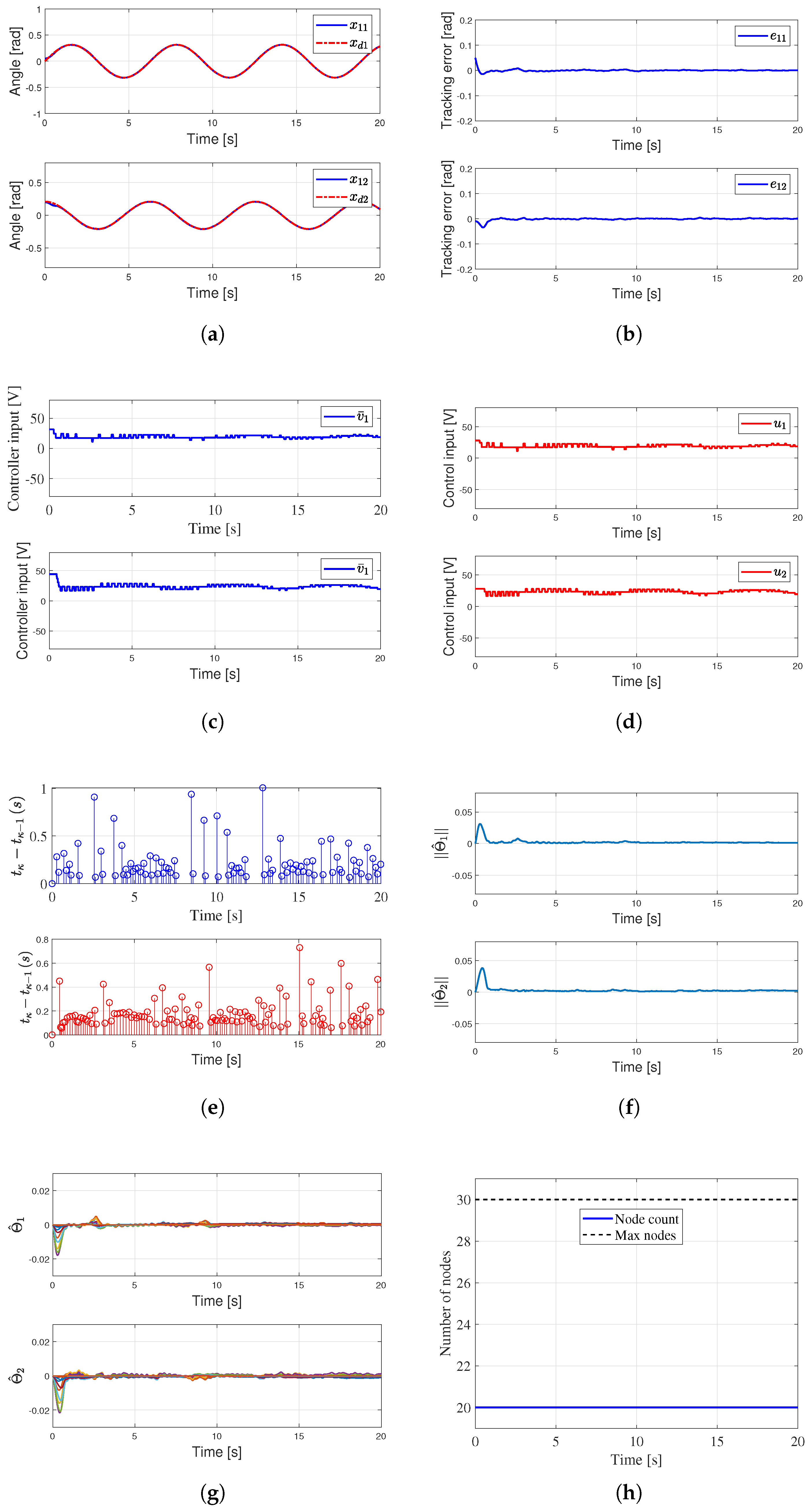
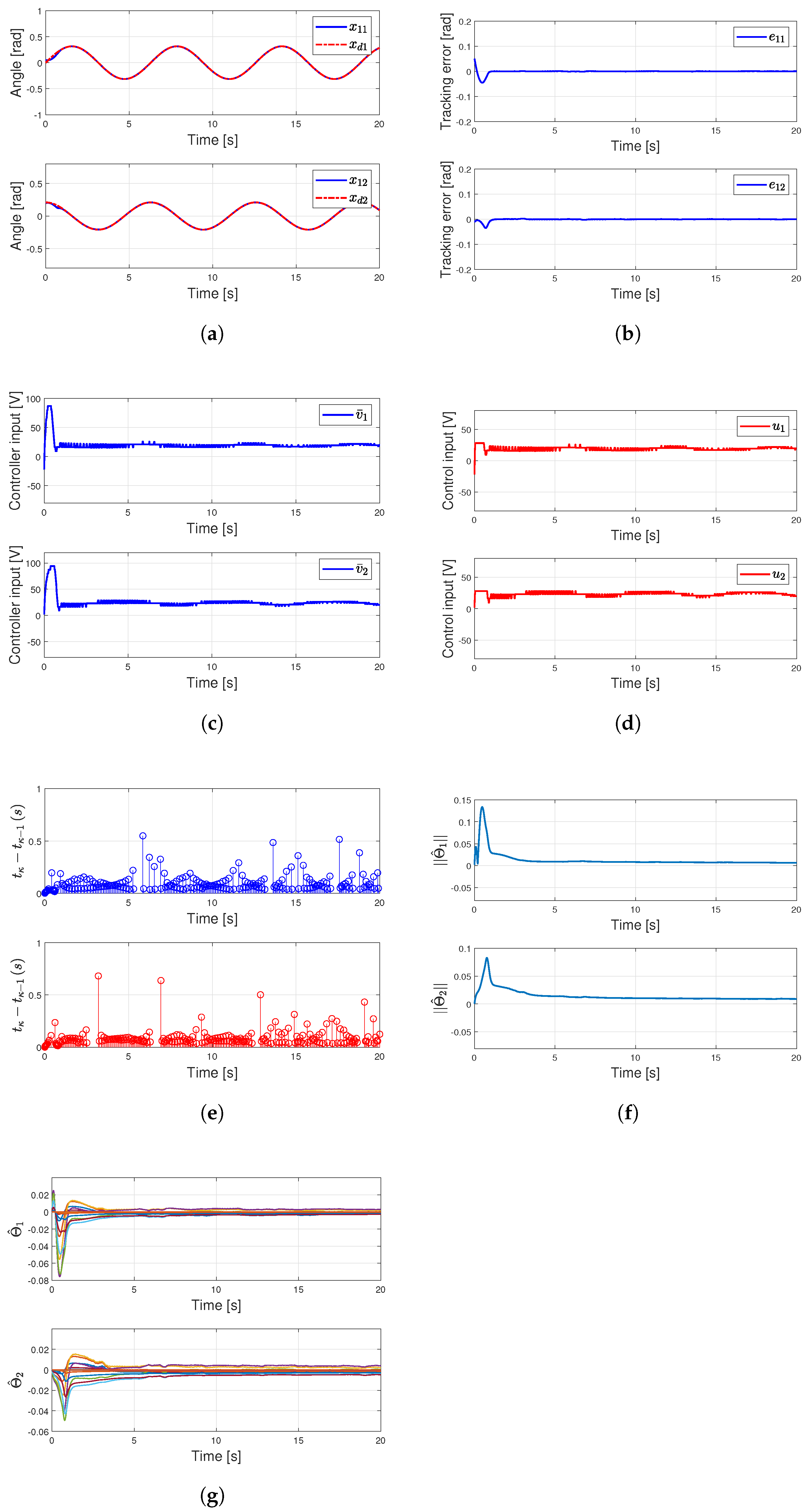
This section presents simulation results evaluating the proposed ADET-CLINC design, as shown in Figure 2. In Figure 2a, the system output consistently and accurately tracks the reference trajectory, thereby minimizing the tracking error, as shown in Figure 2b. Figure 2c illustrates the controller’s dynamic response. Furthermore, as shown in Figure 2d, the system’s control inputs are strictly confined within the specified saturation limits while ensuring stable trajectory tracking. Figure 2e demonstrates the efficiency of the adaptive dynamic event triggering mechanism, which requires only 90 and 113 triggers for the two channels, respectively, thereby significantly reducing the communication load. Finally, Figure 2f,g show the weighted norm of the helicopter’s two angles and the adaptive weights, respectively. Figure 2h shows the curve depicting the number of nodes over time. As can be seen from the figure, the number of nodes in the hidden layer remains constant at 20 and does not reach the maximum of 30. This indicates that the current initial node distribution is already sufficient to cover the state space traversed during system operation; consequently, the distance threshold condition has not been triggered, and no new node growth events have occurred. Taken together, these results confirm that the proposed algorithm effectively achieves the desired control objectives while exhibiting robust tracking performance.

4.2. ADET-INN Without Composite Learning

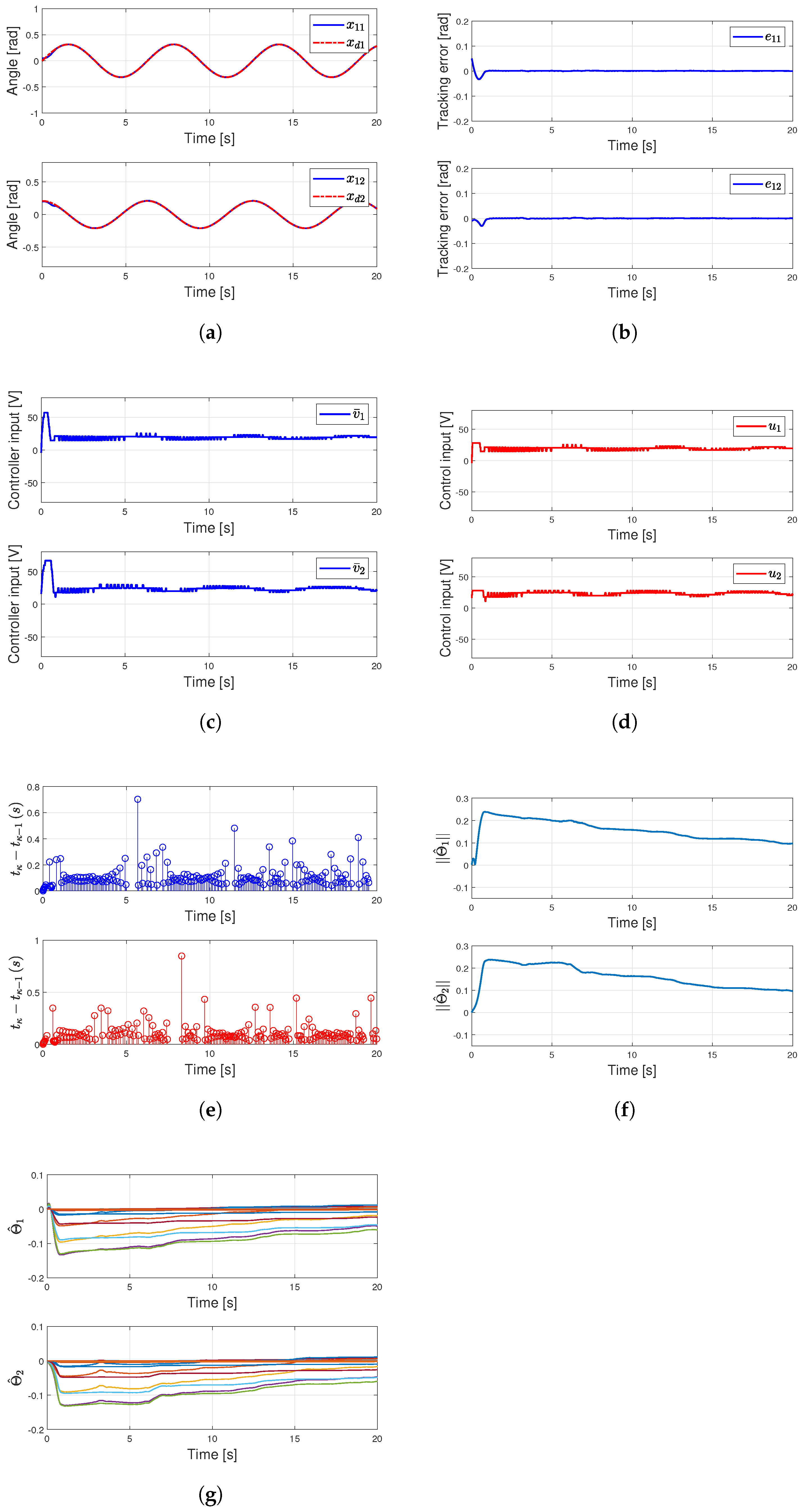
To analyse the impact of the composite learning term on control performance, this paper proposes an ADET-INN without composite learning as a comparison method. This method retains the incremental neural network and the adaptive dynamic event-triggered mechanism, whilst removing only the composite learning term from the weight update law, thereby ensuring that the neural network weights are driven primarily by the current tracking error.

Similar to the previous analysis, Figure 3a,b show the system output and tracking error, respectively; Figure 3c,d show the controller output and actual control input, respectively; Figure 3e shows the event trigger time intervals, with the number of triggers for the two channels being 180 and 186, respectively; Figure 3f,g illustrate the norm of the neural network weights and the changes in the weights, respectively.

As can be seen from the results, the system retains a certain degree of tracking capability even after removing the composite learning term; however, without the assistance of historical prediction error information, the NN relies primarily on instantaneous errors for weight adjustment, which tends to undermine the learning of unknown nonlinear terms. In contrast, the ADET-CLINN proposed in this paper further improves approximation accuracy and control robustness by introducing a composite learning term.

4.3. ADET-CL-RBFNN Without Incremental Learning

To analyse the impact of the incremental node update mechanism on control performance, this paper has set up another set of comparative experiments, namely ADET-CL-RBFNN without Incremental Learning. This method employs the same composite learning weight update mechanism and adaptive dynamic event triggering strategy as the controller proposed in this paper; however, the neural network utilises a fixed-structure RBFNN, no longer adding hidden-layer nodes online based on the system’s operating state. Consequently, this comparative experiment can be used to examine, in isolation, the impact of the incremental learning mechanism on the performance of approximating unknown nonlinearities and trajectory tracking.

Figure 4 shows the simulation results for the ADET-CL-RBFNN without Incremental Learning. As can be seen from Figure 4a, the system output follows the variations in the given reference signal; Figure 4b illustrates the corresponding variations in the tracking error. Figure 4c,d show the controller output signal and the actual control input after input saturation constraints, respectively. Figure 4e is a diagram of event trigger intervals, with the number of triggers for the two control channels being 178 and 180, respectively. Figure 4f,g illustrate the evolution of the NN weight norm and the individual weight components, respectively.

Simulation results indicate that the fixed-structure RBFNN retains a certain degree of compensation capability for unknown dynamics even after incorporating the composite learning strategy, and the system is able to maintain fundamentally stable tracking performance. However, compared with the ADET-CLINN method proposed in this paper, the network structure of this method remains unchanged during simulation, making it difficult to adaptively adjust its approximation capability in response to changes in system state. Consequently, it still exhibits certain shortcomings in terms of tracking accuracy, control input smoothness, and weight update stability. The above results further demonstrate that the incremental learning mechanism can enhance the NN’s adaptability to changes in the state space, thereby improving the controller’s compensation performance for unknown nonlinear dynamics.

4.4. CLINN with Dynamic Event-Triggered Mechanism

To assess the effectiveness of the adaptive dynamic event-triggered mechanism proposed in this paper, CLINN with dynamic event-triggered (CLINN-DET) has been established as a comparison method. The dynamic event-triggered mechanism is based on [19]. This method retains the structure of the composite learning incremental neural network, replacing only the adaptive dynamic event-triggered mechanism proposed in this paper with a conventional dynamic event-triggered mechanism. Consequently, this comparison can provide a relatively direct indication of the impact of adaptive trigger threshold design on communication frequency and control performance.

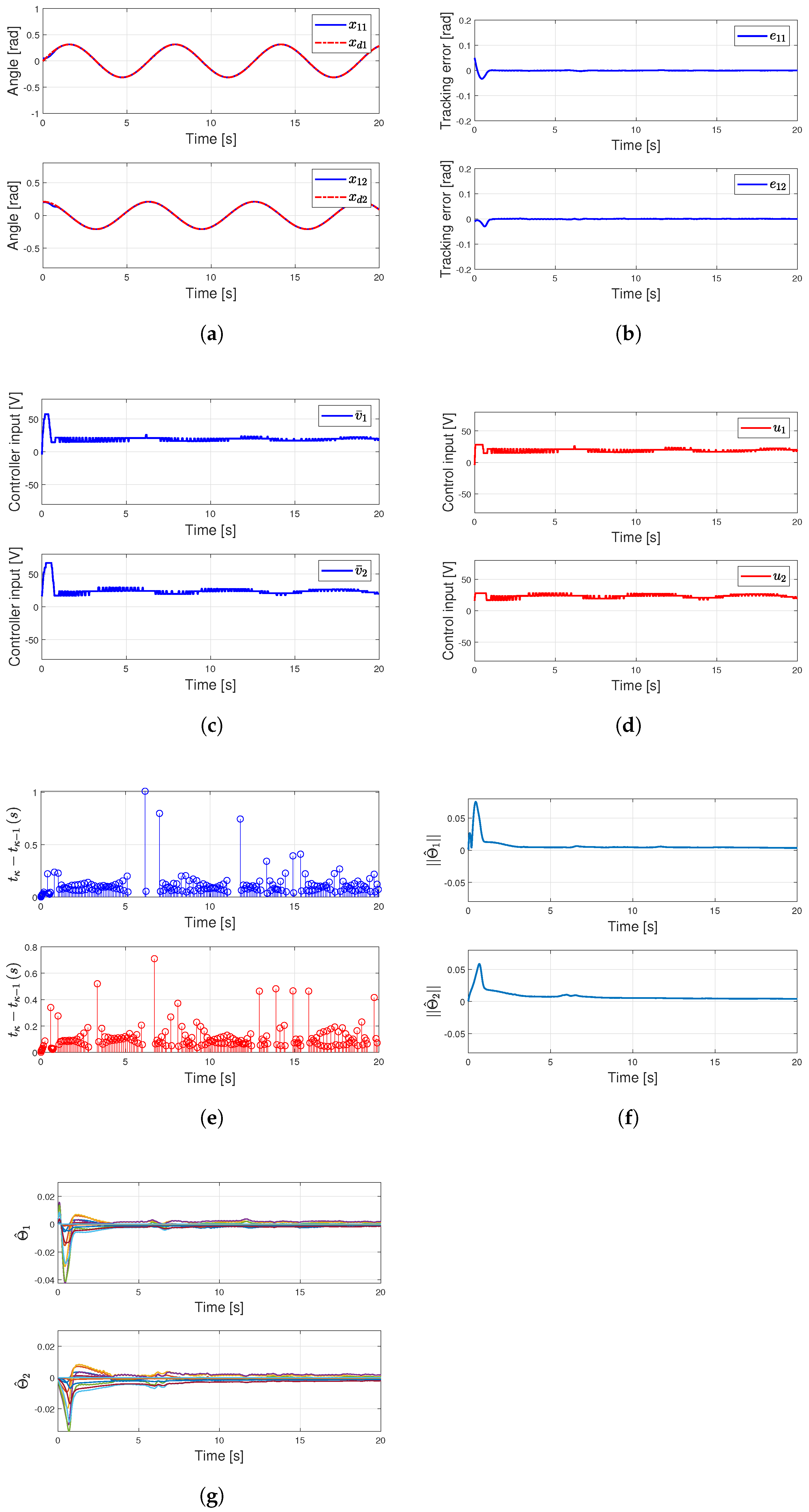
Figure 5a,b show the system output response and tracking error curves, respectively. Figure 5c,d show the controller output and actual control input, respectively. Figure 5e shows the event trigger intervals, with the two control channels triggering 173 and 185 times, respectively. Figure 5f,g illustrate the changes in the norm of the NN weights and the individual weight components, respectively.

The simulation results show that CLINN-DET is still capable of performing basic trajectory tracking, but its trigger frequency is significantly higher than that of the method proposed in this paper. This indicates that conventional dynamic event triggering mechanisms may still generate a large number of redundant updates even after the system has approached a stable state. In contrast, the ADET mechanism proposed in this paper is able to adjust the trigger conditions in response to changes in tracking error, thereby further reducing the communication load whilst ensuring control performance.

4.5. Quantitative Analysis

To further quantitatively evaluate the overall performance of different controllers, this section presents several performance evaluation metrics based on the simulation results described above. These include the root mean square error (RMSE) of the system tracking error and the number of event triggers. These metrics are used to characterise the system’s tracking accuracy, the frequency of event-triggered updates, the trigger interval characteristics, and the consumption of control inputs, respectively.

Table 2. Quantitative performance comparison of different controllers

Method	RMSE $\left({\mathit{e}}_{11}\right)$	RMSE $\left({\mathit{e}}_{11}\right)$	Number of Triggers
ADET-CLINN	0.003815	0.003985	203
ADET-INN without CL	0.004952	0.004779	366
ADET-CL-RBFNN without IL	0.004943	0.004722	358
CLINN-DET	0.006655	0.004251	425

presents the quantitative comparison results of different controllers under the aforementioned metrics. It can be seen that the proposed ADET-CLINN controller is able to effectively reduce the number of event triggers whilst maintaining a small tracking error. This indicates that the proposed method not only exhibits good trajectory tracking performance but also demonstrates superior overall performance in terms of event trigger update frequency.

5. Conclusions

This paper proposed a dynamic event-triggered CLINC controller for a 2-DOF helicopter system subject to system uncertainties, input saturation, and communication constraints. Firstly, a CLINN approach was designed. By introducing estimation error information, this approach improved the adaptive control performance and alleviated the dependence on the classical persistent excitation condition for parameter learning. Meanwhile, an anti-windup auxiliary system was constructed to eliminate the effect of input saturation. Furthermore, an ADET mechanism was introduced to reduce the communication burden between the controller and the actuator. Then, a Lyapunov function was employed to conduct stability analysis, which proved that all signals of the closed-loop system were semi-globally uniformly ultimately bounded. Finally, simulations on the 2-DOF helicopter platform verified the effectiveness and superiority of the proposed algorithm. In the future, our work will focus on experimental validation and further investigation of potential nonlinear phenomena, such as jump resonance and chaos, under a wider range of excitation conditions and parameter variations [28].

References

1. Cao, L.; Zhang, J.; Liu, S.; Zhao, Z. Adaptive neural fault-tolerant control of an uncertain 2-DOF helicopter system with actuator faults and output error constrains. Inst. Eng. Technol. Control Theory Appl. 2023, 17, 1768–1778. [Google Scholar]
2. Yang, G. State filtered disturbance rejection control. Nonlinear Dyn. 2025, 113, 6739–6755. [Google Scholar]
3. Yang, G. Multilayer Neuroadaptive Reinforcement Learning of Disturbed Nonlinear Systems via Actor-Critic Mechanism. IEEE Trans. Autom. Sci. Eng. 2025, 23, 1372–1381. [Google Scholar] [CrossRef] [Scilit]
4. Kumar, E.V.; Raaja, G.S.; Jerome, J. Adaptive PSO for optimal LQR tracking control of 2 DoF laboratory helicopter. Appl. Soft Comput. 2016, 41, 77–90. [Google Scholar] [CrossRef] [Scilit]
5. Zheng, B.; Zhong, Y. Robust attitude regulation of a 3-DOF helicopter benchmark: Theory and experiments. IEEE Trans. Ind. Electron. 2010, 58, 660–670. [Google Scholar] [CrossRef] [Scilit]
6. Wang, B.; Shen, Y.; Zhang, Y. Active fault-tolerant control for a quadrotor helicopter against actuator faults and model uncertainties. Aerosp. Sci. Technol. 2020, 99, 105745. [Google Scholar] [CrossRef] [Scilit]
7. Bi, H.; Zhang, J.; Wang, X.; Liu, S.; Zhao, Z.; Zou, T. Neural network-based adaptive finite-time control for 2-dof helicopter systems with prescribed performance and input saturation. J. Intell. Robot. Syst. 2024, 110, 132. [Google Scholar]
8. Zhao, Z.; Zhang, J.; Liu, Z.; Mu, C.; Hong, K.S. Adaptive neural network control of an uncertain 2-DOF helicopter with unknown backlash-like hysteresis and output constraints. IEEE Trans. Neural Netw. Learn. Syst. 2022, 34, 10018–10027. [Google Scholar]
9. He, W.; Zhang, F.; Zhao, Z.; Yang, C.; Wang, C. Reinforcement dynamic learning-based tracking control strategy for an unknown 2-DOF helicopter system. IEEE Trans. Syst. Man Cybern. Syst. 2025, 55, 6777–6788. [Google Scholar] [CrossRef] [Scilit]
10. Huang, H.; Zhang, T.; Yang, C.; Chen, C.P. Motor learning and generalization using broad learning adaptive neural control. IEEE Trans. Ind. Electron. 2019, 67, 8608–8617. [Google Scholar] [CrossRef] [Scilit]
11. Pan, Y.; Sun, T.; Liu, Y.; Yu, H. Composite learning from adaptive backstepping neural network control. Neural Netw. 2017, 95, 134–142. [Google Scholar] [CrossRef] [Scilit] [PubMed]
12. Fan, Y.; Huang, H.; Yang, C. Fixed-time incremental neural control for manipulator based on composite learning with input saturation. Actuators 2022, 11, 373. [Google Scholar] [CrossRef] [Scilit]
13. Zhao, Z.; Zhang, J.; Chen, S.; He, W.; Hong, K.S. Neural-network-based adaptive finite-time control for a two-degree-of-freedom helicopter system with an event-triggering mechanism. IEEE/CAA J. Autom. Sin. 2023, 10, 1754–1765. [Google Scholar]
14. Zhang, H.; Liu, J. Event-triggered fuzzy flight control of a two-degree-of-freedom helicopter system. IEEE Trans. Fuzzy Syst. 2020, 29, 2949–2962. [Google Scholar]
15. Sun, H.; Hou, L.; Zong, G.; Zhao, X. Continuous-Time/Event-Triggered Decentralized Output Feedback Prescribed-Time Control Applied to a 2-DOF Helicopter. IEEE Trans. Autom. Sci. Eng. 2026, 23, 5828–5838. [Google Scholar]
16. Guo, L.; Chen, J.; Li, R.; Jiang, B. Event-Triggered Federated Reinforcement Broad Learning for Intelligent Fault Diagnosis in Uncrewed Helicopter Swarm Systems. IEEE Trans. Cybern. 2025. early access. [Google Scholar] [CrossRef] [Scilit] [PubMed]
17. Song, X.; Chu, L.; Zhao, Z.; Hong, K.S.; Song, S. Reinforcement Learning-Based Predefined-Time Adaptive Optimized Control for a Two-DOF Helicopter via Event-Triggered Communication. IEEE Trans. Aerosp. Electron. Syst. 2026, 62, 4168–4180. [Google Scholar]
18. Zhao, K.; Huang, Y.; Zhou, Y. Dynamic event-triggered adaptive asymptotic tracking control of uncertain systems with unified prescribed performance. IEEE Trans. Autom. Sci. Eng. 2025, 22, 14752–14762. [Google Scholar] [CrossRef] [Scilit]
19. Cao, L.; Mo, Y.; Xiao, W.; Feng, K.; Wu, Z.; Li, X. Dynamic Event-Triggered Adaptive Broad Learning for a Two-Degree-of-Freedom Helicopter System with Prescribed Performance. Mathematics 2025, 13, 3558. [Google Scholar] [CrossRef] [Scilit]
20. Zhang, J.; Yang, Y.; Zhao, Z.; Hong, K.S. Adaptive neural network control of a 2-DOF helicopter system with input saturation. Int. J. Control Autom. Syst. 2023, 21, 318–327. [Google Scholar]
21. Kiefer, T.; Graichen, K.; Kugi, A. Trajectory Tracking of a 3DOF Laboratory Helicopter Under Input and State Constraints. IEEE Trans. Control Syst. Technol. 2010, 18, 944–952. [Google Scholar]
22. Chen, M.; Yan, K.; Wu, Q. Multiapproximator-Based Fault-Tolerant Tracking Control for Unmanned Autonomous Helicopter With Input Saturation. IEEE Trans. Syst. Man Cybern. Syst. 2022, 52, 5710–5722. [Google Scholar]
23. Shen, H.; Yu, X.; Yan, H.; Park, J.H.; Wang, J. Robust Fixed-Time Sliding Mode Attitude Control for a 2-DOF Helicopter Subject to Input Saturation and Prescribed Performance. IEEE Trans. Transp. Electrif. 2025, 11, 1223–1233. [Google Scholar]
24. Wang, Y.; Zhang, X.; Li, A.; Feroskhan, M. Predefined-Time Adaptive Flight Control of a Coaxial Compound Helicopter Against Input Saturation and Perturbations. IEEE Trans. Aerosp. Electron. Syst. 2026, 62, 2040–2056. [Google Scholar]
25. Zhao, Z.; Zhang, D.; Wu, J.; Liu, Z.; Wang, M.; Hong, K.S. Disturbance observer-based neural network control of a 2-dof helicopter system with input saturation and output constraints. IEEE Trans. Syst. Man Cybern. Syst. 2025, 55, 3152–3162. [Google Scholar] [CrossRef] [Scilit]
26. Cao, S.; Sun, L.; Jiang, J.; Zuo, Z. Reinforcement Learning-Based Fixed-Time Trajectory Tracking Control for Uncertain Robotic Manipulators With Input Saturation. IEEE Trans. Neural Netw. Learn. Syst. 2023, 34, 4584–4595. [Google Scholar] [PubMed]
27. Tee, K.P.; Ge, S.S. Control of nonlinear systems with partial state constraints using a barrier Lyapunov function. Int. J. Control 2011, 84, 2008–2023. [Google Scholar] [CrossRef] [Scilit]
28. Fortuna, L.; Buscarino, A. Nonlinear Resonance from Circuits to Systems; World Scientific: Hackensack, NJ, USA, 2025; Volume 100. [Google Scholar]
Figure 1. The flowchart of the control algorithm proposed in this study.
Mathematics 14 02275 g001
Figure 2. The simulation results for the control performance of ADET-CLINN. (a) Helicopter system output tracking response. (b) Helicopter system error response. (c) Helicopter system controller input. (d) Helicopter system control input. (e) Event trigger interval for controller input. (f) The weight norm of an INN based on CL. (g) The weight of an INN based on CL. (h) Curve showing the change in the number of nodes over time.
Mathematics 14 02275 g002
Figure 3. The simulation results for the control performance of ADET-INN without composite learning. (a) Helicopter system output tracking response. (b) Helicopter system error response. (c) Helicopter system controller input. (d) Helicopter system control input. (e) Event trigger interval for controller input. (f) The weight norm of an INN based on CL. (g) The weight of an INN based on CL.
Mathematics 14 02275 g003
Figure 4. The simulation results for the control performance of ADET-CL-RBFNN without incremental learning. (a) Helicopter system output tracking response. (b) Helicopter system error response. (c) Helicopter system controller input. (d) Helicopter system control input. (e) Event trigger interval for controller input. (f) The weight norm of an INN based on CL. (g) The weight of an INN based on CL.
Mathematics 14 02275 g004
Figure 5. The simulation results for the control performance of DET-ABLNN. (a) Helicopter system output tracking response. (b) Helicopter system error response. (c) Helicopter system controller input. (d) Helicopter system control input. (e) Event trigger interval for controller input. (f) The weight norm of the ABLNN. (g) The weight of the ABLNN.
Mathematics 14 02275 g005