On Some Milne–Mercer-Type Inequalities via Atangana–Baleanu Conformable Fractional Integrals for h-Convex Functions

Abstract

In this paper, we establish new Milne–Mercer-type inequalities via Atangana–Baleanu conformable fractional integral operators for differentiable functions whose derivatives in absolute value are h-convex. First, we derive a novel identity involving the Atangana–Baleanu conformable fractional integral operators. Then, by employing the properties of h-convex functions and fractional integral operators, several new inequalities of the Milne–Mercer type are obtained. The results presented in this paper extend and generalize various previously known inequalities, including classical Milne inequalities, Riemann–Liouville fractional integral inequalities, and conformable fractional integral inequalities. Moreover, several special cases are discussed to demonstrate the generality and applicability of the obtained results. The findings provide new refinements in the theory of fractional integral inequalities and contribute to the development of convex analysis within fractional frameworks.

1. Introduction

Integral inequalities constitute an important branch of mathematical analysis and have attracted considerable attention due to their wide applications in numerical integration, approximation theory, optimization, and differential equations. Among the most influential inequalities are the Hermite–Hadamard, Jensen, Mercer, Simpson, Ostrowski, and Milne inequalities, which provide effective tools for estimating integrals and measuring approximation errors.

The concept of convexity plays a central role in the development of such inequalities. In recent years, several generalized convexity classes have been introduced to obtain more flexible and comprehensive inequalities. Among them, h-convex functions form a broad framework that includes many important subclasses such as ordinary convex functions, P-convex functions, and s-convex functions as special cases. The theory of h-convexity was systematically investigated by Varošanec and has since become a useful tool for establishing generalized integral inequalities.

On the other hand, fractional calculus has emerged as a powerful mathematical discipline for modeling memory and hereditary effects appearing in various scientific and engineering phenomena. Classical fractional operators such as the Riemann–Liouville and Caputo operators have been extensively studied. However, these operators possess singular kernels, which may limit their applicability in certain physical models. To overcome this difficulty, Atangana and Baleanu introduced a new class of fractional operators with non-singular and non-local kernels, now known as the Atangana–Baleanu fractional operators [1,2]. These operators have generated significant interest and have led to numerous investigations concerning fractional differential equations and fractional integral inequalities [3,4,5].

Motivated by the success of AB operators, several authors established new integral inequalities in the AB fractional setting. For example, Set et al. [5,6], Butt et al. [3,7], Kashuri [8], Karim et al. [9], Kermausuor and Nwaeze [10], and Kermausuor et al. [4] derived various Hermite–Hadamard-, Mercer-, and Ostrowski-type inequalities involving Atangana–Baleanu fractional integral operators. In particular, Jiu et al. [11] established Jensen–Mercer-type inequalities in the framework of Atangana–Baleanu fractional operators, while Tariq et al. [12,13] developed several Simpson–Mercer-type and modified integral inequalities in the same setting.

Recently, Milne-type inequalities have received increasing attention due to their close relationship with numerical quadrature formulas and approximation theory. Djenaoui and Meftah [14] established Milne-type inequalities for differentiable s-convex functions in the classical setting. Subsequently, Budak et al. [5] obtained fractional Milne-type inequalities involving Riemann–Liouville fractional integrals. Later, Çelik et al. [15] extended these results to conformable fractional integral operators. More recently, Munir et al. [16] investigated Milne-type inequalities for several classes of generalized convex functions, while Haider et al. and Budak et al. further developed Milne-type inequalities in tempered and generalized fractional settings.

The combination of Mercer-type techniques with fractional operators has also proved fruitful. Mercer’s celebrated refinement of Jensen’s inequality [17] has inspired numerous Mercer-type integral inequalities. Very recently, Benaissa and Sarikaya [18] established Milne–Mercer-type inequalities for h-convex functions and demonstrated that Mercer-type arguments can produce sharper and more flexible estimates than classical Milne inequalities.

Nevertheless, despite the rapid development of both Atangana–Baleanu fractional inequalities and Milne–Mercer-type inequalities, there remain very few results concerning Milne–Mercer-type inequalities involving Atangana–Baleanu conformable fractional integral operators. In particular, to the best of our knowledge, no study has investigated Milne–Mercer-type inequalities for h-convex functions within the framework of Atangana–Baleanu conformable fractional integrals.

Since the Atangana–Baleanu operator incorporates non-singular memory effects while the conformable parameter provides additional flexibility in describing fractional behavior, combining these two structures is mathematically meaningful and leads to a broader family of fractional inequalities.

The purpose of this paper is therefore to establish new Milne–Mercer-type inequalities via Atangana–Baleanu conformable fractional integral operators for differentiable functions whose derivatives in absolute value are h-convex. First, a new identity associated with the ABConf fractional operator is derived. Then, by combining the Jensen–Mercer inequality with the h-convexity property, several new Milne–Mercer-type inequalities are established.

To better illustrate the novelty of the present work, Table 1 compares the proposed framework with several closely related Milne-type inequalities available in the literature.

Table 1. Comparison of the present work with related Milne-type inequalities.

Comparison with Existing Literature and Main Contributions
Reference	Mercer Refinement	h-Convexity	AB Kernel	Conformable Operator
Budak et al. [19]	No	No	No	No
Çelik et al. [15]	No	No	No	Yes
Benaissa and Sarikaya [18]	Yes	Yes	No	No
Present paper	Yes	Yes	Yes	Yes

As shown in Table 1, the present paper simultaneously combines Mercer refinement, h-convexity, Atangana–Baleanu non-singular kernels, and conformable fractional operators within a unified framework. Based on this framework, the main contributions of the paper are as follows. First, a new identity involving Atangana–Baleanu conformable fractional integral operators is established. Second, new Milne–Mercer-type inequalities are derived for differentiable functions whose derivatives in absolute value are h-convex. Third, the obtained results recover and extend several previously known inequalities, including classical Milne inequalities, Riemann–Liouville fractional inequalities, conformable fractional inequalities, Atangana–Baleanu fractional inequalities, and Milne–Mercer-type inequalities as particular cases. These recoveries demonstrate the flexibility, applicability, and unifying nature of the proposed approach.

The remainder of this paper is organized as follows. Section 2 presents the main results together with their proofs. Section 3 discusses special cases and recoveries of known inequalities. Section 4 provides numerical verification and gap-sensitivity analysis. Finally, concluding remarks and future research directions are provided in Section 5.

Definition 1.

A function $f:\left[a,b\right]\to \mathbb{R}$ is called convex on $\left[a,b\right]$ for all $\left(x,y\right)\in$ $\left[a,b\right]$ and $t\in \left[0,1\right]$ if it satisfies the following inequality:

$$f\left(tx+\left(1-t\right)y\right)\le tf\left(x\right)+\left(1-t\right)f\left(y\right)$$

holds.

Definition 2.

Let $h:\left[a,b\right]\to \mathbb{R}$ be a non-negative function, $h\ne 0.$ We sat that $f:\left[a,b\right]\to \mathbb{R}$ is an h-convex function, if f is non-negative and for all $x,y\in \left[a,b\right],$ $\lambda \in \left(0,1\right)$ we have

$$f\left(tx+\left(1-t\right)y\right)\le h\left(t\right)f\left(x\right)+h\left(1-t\right)f\left(y\right).$$

If the inequality is reversed, then f is said to be h-concave.

By setting

• $h\left(t\right)=t,$ Definition 2 reduces to convex function.
• $h\left(t\right)=1,$ Definition 2 reduces to P-convex.
• $h\left(t\right)=t^s,$ Definition 2 reduces to s-convex function.

In 2003, Mercer [17] introduced a refined version of the classical Jensen inequality, now known as the Jensen–Mercer inequality, stated as follows.

For a convex mapping $f:\left[a,b\right]\to \mathbb{R},$ the following inequality holds for each $x_j\in \left[a,b\right]$:

$$f\left(a+b-{\displaystyle \sum _{j=1}^n}{u}_j{x}_j\right)\le f\left(a\right)+f\left(b\right)-{\displaystyle \sum _{j=1}^n}{u}_{j}f\left(x_j\right),$$

where $u_j\in \left[0,1\right]$ and ${\sum }_{j=1}^n{u}_j=1.$

Milne’s formula, which is of the open type, is parallel to Simpson’s formula, which is of the closed type, since they are held under the same conditions.

Suppose that $f:\left[a,b\right]\to \mathbb{R}$ is a four times continuously differentiable mapping on $\left(a,b\right)$ and let ${∥f^{\left(4\right)}∥}_{\infty }={\displaystyle \underset{t\infty \left(a,b\right)}{sup}}\left|f^{\left(4\right)}\left(t\right)\right|<\infty .$ Then the following inequality holds:

$$\left|{\displaystyle \frac{1}{3}}\left[2f\left(a\right)-f\left({\displaystyle \frac{a+b}{2}}\right)+2f\left(b\right)\right]-{\displaystyle \frac{1}{b-a}}{\int }_a^{b}f\left(t\right)dt\right|\le {\displaystyle \frac{7{\left(b-a\right)}^4}{23040}}∥f^{\left(4\right)}∥.$$

Recently, Atangana and Baleanu proposed a new fractional derivative operator which also over comes this deficiency. Atangana and Baleanu introduced the derivative operator both in the Caputo–Fabrizio and Riemann–Liouville sense:

Definition 3

([1]). Let $f\in H^1\left(a,b\right),$ $\eta \in \left[0,1\right]$ and $b>a.$ Then the new fractional derivative is defined as

$${}^{ABC}{}_{a}D^{\eta }\left[f\left(t\right)\right]={\displaystyle \frac{B\left(\eta \right)}{1-\eta }}{\int }_a^t{f}^{\prime }\left(s\right)E_{\eta }\left[{\displaystyle \frac{-\eta }{1-\eta }}{\left(t-s\right)}^{\eta }\right]ds.$$

Definition 4

([1]). Let $f\in H^1\left(a,b\right),$ $\eta \in \left[0,1\right]$ and $b>a.$ Then the new fractional derivative is defined as

$${}^{ABC}{}_{a}D^{\eta }\left[f\left(t\right)\right]={\displaystyle \frac{B\left(\eta \right)}{1-\eta }}{\displaystyle \frac{d}{dt}}{\int }_a^{t}f\left(s\right)E_{\eta }\left[{\displaystyle \frac{-\eta }{1-\eta }}{\left(t-s\right)}^{\eta }\right]ds.$$

In the same paper, they give the corresponding Atangana–Baleanu fractional integral operator as follows.

Definition 5

([1]). Let $f\in H^1\left(a,b\right),$ $\eta \in \left[0,1\right]$ and $b>a,$ then its fractional integral operator with non-local kernel is defined as

$${}^{ABC}{}_{a^{+}}I^{\eta }\left\{f\left(t\right)\right\}={\displaystyle \frac{1-\eta }{B\left(\eta \right)}}f\left(t\right)+{\displaystyle \frac{\eta }{B\left(\eta \right)\Gamma \left(\eta \right)}}{\int }_a^{t}f\left(s\right){\left(t-s\right)}^{\eta -1}ds,$$

where $\Gamma \left(\eta \right)$ is the Gamma function.

Definition 6

([1]). Let $f\in H^1\left(a,b\right),$ $\eta \in \left[0,1\right]$ and $b>a,$ then the right-hand side of AB-fractional integral operator is

$${}^{AB}{}_{b^{-}}I^{\eta }\left\{f\left(t\right)\right\}={\displaystyle \frac{1-\eta }{B\left(\eta \right)}}f\left(t\right)+{\displaystyle \frac{\eta }{B\left(\eta \right)\Gamma \left(\eta \right)}}{\int }_t^{b}f\left(s\right){\left(s-t\right)}^{\eta -1}ds.$$

Besides the development of Atangana–Baleanu fractional operators, another active research direction concerns conformable fractional operators. The conformable approach introduces an additional parameter that preserves many useful properties of classical calculus while retaining the non-local characteristics of fractional analysis.

Due to their simple structure and analytical flexibility, conformable fractional operators have been successfully applied in fractional differential equations, approximation theory, and integral inequalities.

In particular, they provide an effective bridge between classical and fractional frameworks and often yield more tractable representations than traditional fractional operators.

Motivated by these advantages, Jarad et al. [20] introduced conformable fractional integral operators, which extend the classical Riemann–Liouville fractional integrals by incorporating a conformable parameter. These operators have subsequently become an important tool for establishing various fractional integral inequalities.

Definition 7

([20]). The fractional conformable integral operator $I_{a^{+}}^{\beta }f\left(x\right)$ and $I_{b^{-}}^{\beta }f\left(x\right)$ of order $\beta \in \mathbb{C}$, $Re\left(\beta \right)>0$ and $\alpha \in \left(0,1\right]$ are given by

$$\left({}^{C}I_{a^{+}}^{\beta ,\alpha }f\right)\left(t\right)={\displaystyle \frac{1}{\Gamma \left(\beta \right)}}{\int }_a^t{\displaystyle \frac{1}{{\left(s-a\right)}^{1-\alpha }}}{\left[{\displaystyle \frac{{\left(t-a\right)}^{\alpha }-{\left(s-a\right)}^{\alpha }}{\alpha }}\right]}^{\beta -1}f\left(s\right)ds,$$

and

$$\left({}^{C}I_{b^{-}}^{\beta ,\alpha }f\right)\left(t\right)={\displaystyle \frac{1}{\Gamma \left(\beta \right)}}{\int }_t^b{\displaystyle \frac{1}{{\left(b-s\right)}^{1-\alpha }}}{\left[{\displaystyle \frac{{\left(b-t\right)}^{\alpha }-{\left(b-s\right)}^{\alpha }}{\alpha }}\right]}^{\beta -1}f\left(s\right)ds.$$

For $\alpha =1,$ the previous operators are reduced to Riemann–Liouville fractional operators with order $\beta >0$ as follows:

$$\left(J_{a^{+}}^{\beta }f\right)\left(t\right)={\displaystyle \frac{1}{\Gamma \left(\beta \right)}}{\int }_a^t{\left(t-s\right)}^{\beta -1}f\left(s\right)ds,t>a,$$

and

$$\left(J_{b^{-}}^{\beta }f\right)\left(t\right)={\displaystyle \frac{1}{\Gamma \left(\beta \right)}}{\int }_t^b{\left(s-t\right)}^{\beta -1}f\left(s\right)ds,t<b.$$

The beta-Euler function $\beta \left(·,·\right)$ is defined for any $p,q>0$ as follows:

$$\beta \left(p,q\right)={\int }_0^1{\left(1-y\right)}^{q-1}{y}^{p-1}dy.$$

In 2022, Djenaoui and Meftah [14] presented a Milne’s inequality for convex functions with Riemann integral as follows:

$$\left|{\displaystyle \frac{1}{3}}\left[2f\left(a\right)-f\left({\displaystyle \frac{a+b}{2}}\right)+2f\left(b\right)\right]-{\displaystyle \frac{1}{b-a}}{\int }_a^{b}f\left(t\right)dt\right|\le {\displaystyle \frac{5\left(b-a\right)}{24}}\left(\left|f^{\prime }\left(a\right)\right|+\left|f^{\prime }\left(b\right)\right|\right).$$

In 2023, Budak et al. [19] established a fractional Milne-type inequality for convex functions using Riemann–Liouville integral operators:

$$\begin{array}{ccc}& & \left|{\displaystyle \frac{1}{3}}\left[2f\left(a\right)-f\left({\displaystyle \frac{a+b}{2}}\right)+2f\left(b\right)\right]-{\displaystyle \frac{2^{\beta -1}\Gamma \left(\beta +1\right)}{b-a}}\left[\left(J_{{{\displaystyle \frac{a+b}{2}}}^{+}}^{\beta }f\right)\left(b\right)+\left(J_{{{\displaystyle \frac{a+b}{2}}}^{-}}^{\beta }f\right)\left(a\right)\right]\right|\hfill \\ & \le & {\displaystyle \frac{\left(4\beta +1\right)\left(b-a\right)}{12\left(\beta +1\right)}}\left(\left|f^{\prime }\left(a\right)\right|+\left|f^{\prime }\left(b\right)\right|\right).\hfill \end{array}$$

In 2024, Çelik et al. [15] showed that the Milne-type inequality for conformable fractional integral as follows:

$$\begin{array}{ccc}& & \left|{\displaystyle \frac{1}{3{\alpha }^{\beta }}}\left[2f\left(a\right)-f\left({\displaystyle \frac{a+b}{2}}\right)+2f\left(b\right)\right]\right.\hfill \\ & & \left.-{\displaystyle \frac{2^{\alpha \beta -1}\Gamma \left(\beta +1\right)}{{\left(b-a\right)}^{\alpha \beta }}}\left[\left({}^{\beta }J_{a^{+}}^{\alpha }f\right)\left({\displaystyle \frac{a+b}{2}}\right)+\left({}^{\beta }J_{b^{-}}^{\alpha }f\right)\left({\displaystyle \frac{a+b}{2}}\right)\right]\right|\hfill \\ & \le & {\displaystyle \frac{\left(b-a\right)}{12}}\left({\displaystyle \frac{3B\left(\beta +1,\frac{1}{\alpha }\right)+\alpha }{{\alpha }^{\beta +1}}}\right)\left(\left|f^{\prime }\left(a\right)\right|+\left|f^{\prime }\left(b\right)\right|\right)\hfill \end{array}$$

where $\alpha ,\beta >0,B\left(·,·\right)$ and $\Gamma$ are Euler Beta and Gamma functions, respectively.

In 2026, Benaissa and Sarikaya [18] presented the Milne–Mercer inequality for h-convex function:

$$\begin{array}{ccc}& & \left|{\displaystyle \frac{1}{3}}\left[2f\left(a+b-y\right)-f\left(a+b-{\displaystyle \frac{x+y}{2}}\right)+2f\left(a+b-x\right)\right]\right.\hfill \\ & & \left.-{\displaystyle \frac{2^{\alpha \rho -1{\rho }^{\alpha }}\Gamma \left(\alpha +1\right)}{{\left(y-x\right)}^{\alpha \rho }}}\left[\left({}^{\rho }{J}_{a+b-{{\displaystyle \frac{x+y}{2}}}^{+}}^{\alpha }f\right)\left(a+b-x\right)+\left({}^{\rho }{J}_{a+b-{{\displaystyle \frac{x+y}{2}}}^{-}}^{\alpha }f\right)\left(a+b-y\right)\right]\right|\hfill \\ & \le & {\displaystyle \frac{y-x}{4}}\left[\left|f^{\prime }\left(a+b-y\right)\right|+\left|f^{\prime }\left(a+b-x\right)\right|\right]{\int }_0^1\left({\displaystyle \frac{4}{3}}-{\left(1-t^{\rho }\right)}^{\alpha }\right)\left[h\left(t\right)+2h\left({\displaystyle \frac{1}{2}}\right)h\left(1-t\right)\right]dt\hfill \end{array}$$

for $\alpha >0, \rho \in \left(0,1\right]$ and $x,y\in \left[a,b\right]$ where $x<y$ and $\left|f^{\prime }\right|$ is a h-convex mapping on $\left[a,b\right].$

Throughout the paper, we use the following parameters:

Let $0\le a<b,$ and $f:\left[a,b\right]\to \mathbb{R}$ be a function such that the involved integrals exist.

$\eta \in \left[0,1\right]$ denotes the Atangana–Baleanu (AB) fractional order; $\alpha \in \left(0,1\right]$ denotes the Conformable parameter.

$B\left(\eta \right)>0$ is the AB normalization function satisfying $B\left(0\right)=B\left(1\right)=1.$

We denote by $\Gamma \left(·\right)$ the Gamma function and by $E_{\eta }\left(·\right)$ the one-parameter Mittag–Leffler function.

In [21], Lo denoted the new operator with AB-conformable fractional integrals.

Definition 8.

Let $f:\left[a,b\right]\to \mathbb{R}$ be a function and $\eta \in \left[0,1\right], \alpha \in \left(0,1\right]$

We denote by

$$\begin{array}{ccc}& & {}^{ABConf}{}_{a^{+}}I^{\eta ,\alpha }\left\{f\left(t\right)\right\}\hfill \\ & =& {\displaystyle \frac{1-\eta }{B\left(\eta \right)}}f\left(t\right)+{\displaystyle \frac{\eta }{B\left(\eta \right)\Gamma \left(\eta \right)}}{\int }_a^t{\displaystyle \frac{1}{{\left(s-a\right)}^{1-\alpha }}}{\left[{\displaystyle \frac{{\left(t-a\right)}^{\alpha }-{\left(s-a\right)}^{\alpha }}{\alpha }}\right]}^{\eta -1}f\left(s\right)ds,\hfill \end{array}$$

and

$$\begin{array}{ccc}& & {}^{ABConf}{}_{b^{-}}I^{\eta ,\alpha }\left\{f\left(t\right)\right\}\hfill \\ & =& {\displaystyle \frac{1-\eta }{B\left(\eta \right)}}f\left(t\right)+{\displaystyle \frac{\eta }{B\left(\eta \right)\Gamma \left(\eta \right)}}{\int }_t^b{\displaystyle \frac{1}{{\left(b-s\right)}^{1-\alpha }}}{\left[{\displaystyle \frac{{\left(b-t\right)}^{\alpha }-{\left(b-s\right)}^{\alpha }}{\alpha }}\right]}^{\eta -1}f\left(s\right)ds.\hfill \end{array}$$

Remark 1.

Let $\eta \in \left[0,1\right]$ and set $\alpha =1.$ Then for all $s\in \left[a,b\right]$

$$\left({}^{ABConf}{}_{a^{+}}I^{\eta ,1}\right)\left\{f\left(t\right)\right\}=\left(AB{}_{a^{+}}I^{\eta }\right)\left\{f\left(t\right)\right\},$$

$$\left({}^{ABConf}{}_{b^{-}}I^{\eta ,1}\right)\left\{f\left(t\right)\right\}=\left(AB{}_{b^{-}}I^{\eta }\right)\left\{f\left(t\right)\right\}.$$

Remark 2.

Let $\alpha \in \left(0,1\right]$ and set $\eta =1$. Using $B\left(1\right)=1$ and $\Gamma \left(1\right)=1,$ we obtain

$${}^{ABConf}{}_{a^{+}}I^{1,\alpha }\left\{f\left(t\right)\right\}={\int }_a^t{\displaystyle \frac{1}{{\left(s-a\right)}^{1-\alpha }}}f\left(s\right)ds,$$

and

$${}^{ABConf}{}_{b^{-}}I^{1,\alpha }\left\{f\left(t\right)\right\}={\int }_t^b{\displaystyle \frac{1}{{\left(b-s\right)}^{1-\alpha }}}f\left(s\right)ds.$$

That is, ${}^{ABConf}{I}^{1,\alpha }\left\{f\left(t\right)\right\}$ coincides with the conformable integral of order 1 with parameter $\alpha .$

Remark 3.

If $\alpha =1$ and $\eta =1,$ then ${}^{ABConf}{I}^{1,\alpha }\left\{f\left(t\right)\right\}$ integral reduces the classical (Riemann) integral over the same endpoints.

Remark 4.

Since $0<\alpha \le 1,$ the factor ${\left(s-a\right)}^{\alpha -1}$ is locally integrable near $s=a.$ Moreover, $0<\eta \le 1$ implies that the factor ${\left[{\left(t-a\right)}^{\alpha }-{\left(s-a\right)}^{\alpha }\right]}^{\eta -1}$ remains integrable near $s=t.$ Hence the Atangana–Baleanu conformable fractional integral operators introduced in Definition 8 are well defined for every $f\in L^1\left(\left[a,b\right]\right).$

2. Main Result

Lemma 1.

Let $f:\left[a,b\right]\to \mathbb{R}$ with $0\le a<b,$ $\eta \in \left[0,1\right]$ and $\alpha \in \left(0,1\right]$ and f is differentiable and $f^{\prime }\in L^1.$ Then the following identity is valid for Atangana–Baleanu conformable fractional integral operators:

$$\begin{array}{ccc}& & {\displaystyle \frac{1}{3}}\left[2f\left(a+b-m\right)-f\left(a+b-{\displaystyle \frac{m+n}{2}}\right)+2f\left(a+b-n\right)\right]{\displaystyle \frac{{\left(n-m\right)}^{\alpha \eta }}{B\left(\eta \right)\Gamma \left(\eta \right)}}\hfill \\ & & +{\displaystyle \frac{2^{\alpha \eta -1}{\alpha }^{\eta }\left(1-\eta \right)}{B\left(\eta \right)}}\left[f\left(a+b-n\right)+f\left(a+b-m\right)\right]\hfill \\ & & -2^{\alpha \eta -1}{\alpha }^{\eta }\left[{{}^{ABConf}}_{a+b-{{\displaystyle \frac{m+n}{2}}}^{+}}{I}^{\eta ,\alpha }\left\{f\left(a+b-m\right)\right\}{{+}^{ABConf}}_{a+b-{{\displaystyle \frac{m+n}{2}}}^{-}}{I}^{\eta ,\alpha }\left\{f\left(a+b-n\right)\right\}\right]\hfill \\ & =& {\displaystyle \frac{{\left(n-m\right)}^{\alpha \eta +1}}{4B\left(\eta \right)\Gamma \left(\eta \right)}}\left\{{\int }_0^1\left[{\displaystyle \frac{4}{3}}-{\left(1-t^{\alpha }\right)}^{\eta }\right]f^{\prime }\left(a+b-\left[\left({\displaystyle \frac{1+t}{2}}\right)m+\left({\displaystyle \frac{1-t}{2}}\right)n\right]\right)dt\right.\hfill \\ & & \left.-{\int }_0^1\left[{\displaystyle \frac{1}{3}}+{\left(1-{\left(1-t\right)}^{\alpha }\right)}^{\eta }\right]f^{\prime }\left(a+b-\left[\left({\displaystyle \frac{1-t}{2}}\right)m+\left({\displaystyle \frac{1+t}{2}}\right)n\right]\right)dt\right\}.\hfill \end{array}$$

Proof. 

Step 1. By using integration by parts.

$$\begin{array}{ccc}\hfill I_1& =& {\int }_0^1\left[{\displaystyle \frac{4}{3}}-{\left(1-t^{\alpha }\right)}^{\eta }\right]f^{\prime }\left(a+b-\left[\left({\displaystyle \frac{1+t}{2}}\right)m+\left({\displaystyle \frac{1-t}{2}}\right)n\right]\right)dt\hfill \\ & =& {\displaystyle \frac{8f\left(a+b-m\right)}{3\left(n-m\right)}}-{\displaystyle \frac{2f\left(a+b-\frac{m+n}{2}\right)}{3\left(n-m\right)}}\hfill \\ & & -{\displaystyle \frac{2}{n-m}}{\int }_0^{1}f\left(a+b-\left[\left({\displaystyle \frac{1+t}{2}}\right)m+\left({\displaystyle \frac{1-t}{2}}\right)n\right]\right)\left(-\eta \right){\left[1-t^{\alpha }\right]}^{\eta -1}\left(-\alpha \right){\left(t\right)}^{\alpha -1}dt.\hfill \end{array}$$

Step 2. By changing variable $x=a+b-\left[\left({\displaystyle \frac{1+t}{2}}\right)m+\left({\displaystyle \frac{1-t}{2}}\right)n\right],$ we get

$$\begin{array}{ccc}\hfill I_1& =& {\displaystyle \frac{8f\left(a+b-m\right)}{3\left(n-m\right)}}-{\displaystyle \frac{2f\left(a+b-\frac{m+n}{2}\right)}{3\left(n-m\right)}}\hfill \\ & & -{\displaystyle \frac{2\alpha \eta }{n-m}}{\int }_{a+b-{\displaystyle \frac{m+n}{2}}}^{a+b-m}f\left(x\right){\displaystyle \frac{2}{n-m}}{\left[{\displaystyle \frac{2\left(x-\left(a+b-\frac{m+n}{2}\right)\right)}{n-m}}\right]}^{\alpha -1}\hfill \\ & & \times {\left[{\left({\displaystyle \frac{2\left(\left(a+b-m\right)-\left(a+b-\frac{m+n}{2}\right)\right)}{n-m}}\right)}^{\alpha }-{\left({\displaystyle \frac{2\left(x-\left(a+b-\frac{m+n}{2}\right)\right)}{n-m}}\right)}^{\alpha }\right]}^{\eta -1}dx\hfill \end{array}$$

$$\begin{array}{ccc}& =& {\displaystyle \frac{8f\left(a+b-m\right)}{3\left(n-m\right)}}-{\displaystyle \frac{2f\left(a+b-\frac{m+n}{2}\right)}{3\left(n-m\right)}}\hfill \\ & & -{\displaystyle \frac{2^{\alpha \eta +1}{\alpha }^{\eta }\eta }{{\left(n-m\right)}^{\alpha \eta +1}}}{\int }_{a+b-{\displaystyle \frac{m+n}{2}}}^{a+b-m}{\displaystyle \frac{1}{{\left[x-\left(a+b-\frac{m+n}{2}\right)\right]}^{1-\alpha }}}\hfill \\ & & \times {\left[{\displaystyle \frac{{\left[\left(a+b-m\right)-\left(a+b-\frac{m+n}{2}\right)\right]}^{\alpha }-{\left[x-\left(a+b-\frac{m+n}{2}\right)\right]}^{\alpha }}{\alpha }}\right]}^{\eta -1}f\left(x\right)dx\hfill \end{array}$$

Step 3. By Definition 8, the definition of AB-Conf-fractional intergals, then we have

$$\begin{array}{ccc}\hfill I_1& =& {\displaystyle \frac{8f\left(a+b-m\right)}{3\left(n-m\right)}}-{\displaystyle \frac{2f\left(a+b-\frac{m+n}{2}\right)}{3\left(n-m\right)}}\hfill \\ & & +{\displaystyle \frac{\Gamma \left(\eta \right)2^{\alpha \eta +1}{\alpha }^{\eta }\left(1-\eta \right)}{{\left(n-m\right)}^{\alpha \eta +1}}}f\left(a+b-m\right)\hfill \\ & & -{\displaystyle \frac{B\left(\eta \right)\Gamma \left(\eta \right)2^{\alpha \eta +1}{\alpha }^{\eta }}{{\left(n-m\right)}^{\alpha \eta +1}}}{{}^{ABConf}}_{a+b-{{\displaystyle \frac{m+n}{2}}}^{+}}{I}^{\eta ,\alpha }\left\{f\left(a+b-m\right)\right\}.\hfill \end{array}$$

Similarly, let

$$I_2={\int }_0^1\left[{\displaystyle \frac{1}{3}}+{\left(1-{\left(1-t\right)}^{\alpha }\right)}^{\eta }\right]f^{\prime }\left(a+b-\left[\left({\displaystyle \frac{1-t}{2}}\right)m+\left({\displaystyle \frac{1+t}{2}}\right)n\right]\right)dt.$$

By integration by parts and changing variable $x=a+b-\left[\left({\displaystyle \frac{1-t}{2}}\right)m+\left({\displaystyle \frac{1+t}{2}}\right)n\right],$ we get

$$\begin{array}{ccc}\hfill I_2& =& -{\displaystyle \frac{8f\left(a+b-n\right)}{3\left(n-m\right)}}+{\displaystyle \frac{2f\left(a+b-\frac{m+n}{2}\right)}{3\left(n-m\right)}}\hfill \\ & & +{\displaystyle \frac{2}{n-m}}{\int }_0^{1}f\left(a+b-\left[\left({\displaystyle \frac{1-t}{2}}\right)m+\left({\displaystyle \frac{1+t}{2}}\right)n\right]\right)\hfill \\ & & \times \eta {\left[1-{\left(1-t\right)}^{\alpha }\right]}^{\eta -1}\left(-\alpha \right){\left(1-t\right)}^{\alpha -1}\left(-1\right)dt\hfill \\ & =& -{\displaystyle \frac{8f\left(a+b-n\right)}{3\left(n-m\right)}}+{\displaystyle \frac{2f\left(a+b-\frac{m+n}{2}\right)}{3\left(n-m\right)}}\hfill \\ & & +{\displaystyle \frac{2\alpha \eta }{n-m}}{\int }_{a+b-{\displaystyle \frac{m+n}{2}}}^{a+b-n}{\left[{\displaystyle \frac{2\left(\left(a+b-\frac{m+n}{2}\right)-x\right)}{n-m}}\right]}^{\alpha -1}\hfill \\ & & \times {\left[{\left({\displaystyle \frac{2\left(\left(a+b-\frac{m+n}{2}\right)-\left(a+b-n\right)\right)}{n-m}}\right)}^{\alpha }-{\left({\displaystyle \frac{2\left(\left(a+b-\frac{m+n}{2}\right)-x\right)}{n-m}}\right)}^{\alpha }\right]}^{\eta -1}f\left(x\right){\displaystyle \frac{-2}{n-m}}dx\hfill \\ & =& -{\displaystyle \frac{8f\left(a+b-n\right)}{3\left(n-m\right)}}+{\displaystyle \frac{2f\left(a+b-\frac{m+n}{2}\right)}{3\left(n-m\right)}}\hfill \\ & & +{\displaystyle \frac{2^{\alpha \eta +1}{\alpha }^{\eta }\eta }{{\left(n-m\right)}^{\alpha \eta +1}}}{\int }_{a+b-n}^{a+b-{\displaystyle \frac{m+n}{2}}}{\displaystyle \frac{1}{{\left[\left(a+b-\frac{m+n}{2}\right)-x\right]}^{1-\alpha }}}\hfill \\ & & \times {\left[{\displaystyle \frac{{\left[\left(a+b-\frac{m+n}{2}\right)-\left(a+b-n\right)\right]}^{\alpha }-{\left[\left(a+b-\frac{m+n}{2}\right)-x\right]}^{\alpha }}{\alpha }}\right]}^{\eta -1}f\left(x\right)dx.\hfill \end{array}$$

By Definition 8, the definition of AB-Conf-fractional intergals, then we have

$$\begin{array}{ccc}\hfill I_2& =& -{\displaystyle \frac{8f\left(a+b-n\right)}{3\left(n-m\right)}}+{\displaystyle \frac{2f\left(a+b-\frac{m+n}{2}\right)}{3\left(n-m\right)}}\hfill \\ & & -{\displaystyle \frac{\Gamma \left(\eta \right)2^{\alpha \eta +1}{\alpha }^{\eta }\left(1-\eta \right)}{{\left(n-m\right)}^{\alpha \eta +1}}}f\left(a+b-n\right)\hfill \\ & & +{\displaystyle \frac{B\left(\eta \right)\Gamma \left(\eta \right)2^{\alpha \eta +1}{\alpha }^{\eta }}{{\left(n-m\right)}^{\alpha \eta +1}}}{{}^{ABConf}}_{a+b-{{\displaystyle \frac{m+n}{2}}}^{+}}{I}^{\eta ,\alpha }\left\{f\left(a+b-n\right)\right\}.\hfill \end{array}$$

Now, $I_1-I_2$ and multiplying by ${\displaystyle \frac{{\left(n-m\right)}^{\alpha \eta +1}}{4B\left(\eta \right)\Gamma \left(\eta \right)}},$ using the definition of AB-Conf-fractional intergals, we get

$$\begin{array}{ccc}\hfill I_1& =& {\displaystyle \frac{8f\left(a+b-m\right)}{3\left(n-m\right)}}-{\displaystyle \frac{2f\left(a+b-\frac{m+n}{2}\right)}{3\left(n-m\right)}}\hfill \\ & & +{\displaystyle \frac{\Gamma \left(\eta \right)2^{\alpha \eta +1}{\alpha }^{\eta }\left(1-\eta \right)}{{\left(n-m\right)}^{\alpha \eta +1}}}f\left(a+b-m\right)\hfill \\ & & -{\displaystyle \frac{B\left(\eta \right)\Gamma \left(\eta \right)2^{\alpha \eta +1}{\alpha }^{\eta }}{{\left(n-m\right)}^{\alpha \eta +1}}}{{}^{ABConf}}_{a+b-{{\displaystyle \frac{m+n}{2}}}^{+}}{I}^{\eta ,\alpha }\left\{f\left(a+b-m\right)\right\}.\hfill \end{array}$$

$$\begin{array}{ccc}& & {\displaystyle \frac{{\left(n-m\right)}^{\alpha \eta +1}}{4B\left(\eta \right)\Gamma \left(\eta \right)}}\left[I_1-I_2\right]\hfill \\ & =& {\displaystyle \frac{1}{3}}\left[2f\left(a+b-m\right)-f\left(a+b-{\displaystyle \frac{m+n}{2}}\right)+2f\left(a+b-n\right)\right]{\displaystyle \frac{{\left(n-m\right)}^{\alpha \eta }}{B\left(\eta \right)\Gamma \left(\eta \right)}}\hfill \\ & & +{\displaystyle \frac{2^{\alpha \eta -1}{\alpha }^{\eta }\left(1-\eta \right)}{B\left(\eta \right)}}\left[f\left(a+b-n\right)+f\left(a+b-m\right)\right]\hfill \\ & & -2^{\alpha \eta -1}{\alpha }^{\eta }\left[{{}^{ABConf}}_{a+b-{{\displaystyle \frac{m+n}{2}}}^{+}}{I}^{\eta ,\alpha }\left\{f\left(a+b-m\right)\right\}{{+}^{ABConf}}_{a+b-{{\displaystyle \frac{m+n}{2}}}^{-}}{I}^{\eta ,\alpha }\left\{f\left(a+b-n\right)\right\}\right].\hfill \end{array}$$

□

Theorem 1.

Let $f:\left[a,b\right]\to \mathbb{R}$ with $0\le a<b,$ $\eta \in \left[0,1\right]$ and $\alpha \in \left(0,1\right]$ and assume that $h:[0,1]\to [0,\infty )$. If f is differentiable, $f^{\prime }\in L^1\left([a,b]\right),\mathrm{and}],$ then the following Milne–Mercer-type inequality for ABConf fractional operator holds:

$$\begin{array}{ccc}& & \left|{\displaystyle \frac{1}{3}}\left[2f\left(a+b-m\right)-f\left(a+b-{\displaystyle \frac{m+n}{2}}\right)+2f\left(a+b-n\right)\right]{\displaystyle \frac{{\left(n-m\right)}^{\alpha \eta }}{B\left(\eta \right)\Gamma \left(\eta \right)}}\right.\hfill \\ & & +{\displaystyle \frac{2^{\alpha \eta -1}{\alpha }^{\eta }\left(1-\eta \right)}{B\left(\eta \right)}}\left[f\left(a+b-n\right)+f\left(a+b-m\right)\right]\hfill \\ & & \left.-2^{\alpha \eta -1}{\alpha }^{\eta }\left[{{}^{ABConf}}_{a+b-{{\displaystyle \frac{m+n}{2}}}^{+}}{I}^{\eta ,\alpha }\left\{f\left(a+b-m\right)\right\}{{+}^{ABConf}}_{a+b-{{\displaystyle \frac{m+n}{2}}}^{-}}{I}^{\eta ,\alpha }\left\{f\left(a+b-n\right)\right\}\right]\right|\hfill \end{array}$$

$$\begin{array}{ccc}& \le & {\displaystyle \frac{{\left(n-m\right)}^{\alpha \eta +1}}{4B\left(\eta \right)\Gamma \left(\eta \right)}}\hfill \\ & & \times \left\{\left|f^{\prime }\left(a+b-n\right)\right|{\int }_0^{1}h\left({\displaystyle \frac{1}{2}}\right)\left|{\displaystyle \frac{4}{3}}-{\left(1-t^{\alpha }\right)}^{\eta }\right|\left|h\left(1-t\right)\right|+\left|{\displaystyle \frac{1}{3}}+{\left(1-{\left(1-t\right)}^{\alpha }\right)}^{\eta }\right|\left|h\left(t\right)\right|\right.\hfill \\ & & +h\left({\displaystyle \frac{1}{2}}\right)\left|{\displaystyle \frac{1}{3}}+{\left(1-{\left(1-t\right)}^{\alpha }\right)}^{\eta }\right|\left|h\left(1-t\right)\right|dt\hfill \\ & & +\left|f^{\prime }\left(a+b-m\right)\right|{\int }_0^{1}h\left({\displaystyle \frac{1}{2}}\right)\left|{\displaystyle \frac{4}{3}}-{\left(1-t^{\alpha }\right)}^{\eta }\right|\left|h\left(1-t\right)\right|+\left|{\displaystyle \frac{4}{3}}-{\left(1-t^{\alpha }\right)}^{\eta }\right|\left|h\left(t\right)\right|\hfill \\ & & \left.+h\left({\displaystyle \frac{1}{2}}\right)\left|{\displaystyle \frac{1}{3}}+{\left(1-{\left(1-t\right)}^{\alpha }\right)}^{\eta }\right|\left|h\left(1-t\right)\right|dt\right\}.\hfill \end{array}$$

for all $a\le m<n\le b.$

Proof. 

By Lemma 1 and applying the triangle inequality, we have

$$\begin{array}{ccc}& & \left|{\displaystyle \frac{1}{3}}\left[2f\left(a+b-m\right)-f\left(a+b-{\displaystyle \frac{m+n}{2}}\right)+2f\left(a+b-n\right)\right]{\displaystyle \frac{{\left(n-m\right)}^{\alpha \eta }}{B\left(\eta \right)\Gamma \left(\eta \right)}}\right.\hfill \\ & & +{\displaystyle \frac{2^{\alpha \eta -1}{\alpha }^{\eta }\left(1-\eta \right)}{B\left(\eta \right)}}\left[f\left(a+b-n\right)+f\left(a+b-m\right)\right]\hfill \\ & & \left.-2^{\alpha \eta -1}{\alpha }^{\eta }\left[{{}^{ABConf}}_{a+b-{{\displaystyle \frac{m+n}{2}}}^{+}}{I}^{\eta ,\alpha }\left\{f\left(a+b-m\right)\right\}{{+}^{ABConf}}_{a+b-{{\displaystyle \frac{m+n}{2}}}^{-}}{I}^{\eta ,\alpha }\left\{f\left(a+b-n\right)\right\}\right]\right|\hfill \\ & \le & {\displaystyle \frac{{\left(n-m\right)}^{\alpha \eta +1}}{4B\left(\eta \right)\Gamma \left(\eta \right)}}\left\{{\int }_0^1\left|{\displaystyle \frac{4}{3}}-{\left(1-t^{\alpha }\right)}^{\eta }\right|\left|f^{\prime }\left(\left(1-t\right)\left(a+b-{\displaystyle \frac{m+n}{2}}\right)+t\left(a+b-m\right)\right)\right|dt\right.\hfill \\ & & \left.+{\int }_0^1\left|{\displaystyle \frac{1}{3}}+{\left(1-{\left(1-t\right)}^{\alpha }\right)}^{\eta }\right|\left|f^{\prime }\left(t\left(a+b-n\right)+\left(1-t\right)\left(a+b-{\displaystyle \frac{m+n}{2}}\right)\right)\right|dt\right\}\hfill \end{array}$$

$$\begin{array}{ccc}& \le & {\displaystyle \frac{{\left(n-m\right)}^{\alpha \eta +1}}{4B\left(\eta \right)\Gamma \left(\eta \right)}}\left\{\left|f^{\prime }\left(a+b-{\displaystyle \frac{m+n}{2}}\right)\right|{\int }_0^1\left|{\displaystyle \frac{4}{3}}-{\left(1-t^{\alpha }\right)}^{\eta }\right|\left|h\left(1-t\right)\right|dt\right.\hfill \\ & & +\left|f^{\prime }\left(a+b-m\right)\right|{\int }_0^1\left|{\displaystyle \frac{4}{3}}-{\left(1-t^{\alpha }\right)}^{\eta }\right|\left|h\left(t\right)\right|dt\hfill \\ & & +\left|f^{\prime }\left(a+b-n\right)\right|{\int }_0^1\left|{\displaystyle \frac{1}{3}}+{\left(1-{\left(1-t\right)}^{\alpha }\right)}^{\eta }\right|\left|h\left(t\right)\right|dt\hfill \\ & & +f^{\prime }\left(a+b-{\displaystyle \frac{m+n}{2}}\right){\int }_0^1\left|{\displaystyle \frac{1}{3}}+{\left(1-{\left(1-t\right)}^{\alpha }\right)}^{\eta }\right|\left|h\left(1-t\right)\right|dt\hfill \end{array}$$

$$\begin{array}{ccc}& \le & {\displaystyle \frac{{\left(n-m\right)}^{\alpha \eta +1}}{4B\left(\eta \right)\Gamma \left(\eta \right)}}\left\{h\left({\displaystyle \frac{1}{2}}\right)\left[\left|f^{\prime }\left(a+b-n\right)\right|+\left|f^{\prime }\left(a+b-m\right)\right|\right]\right.\hfill \\ & & \times {\int }_0^1\left|{\displaystyle \frac{4}{3}}-{\left(1-t^{\alpha }\right)}^{\eta }\right|\left|h\left(1-t\right)\right|dt\hfill \\ & & +\left|f^{\prime }\left(a+b-m\right)\right|{\int }_0^1\left|{\displaystyle \frac{4}{3}}-{\left(1-t^{\alpha }\right)}^{\eta }\right|\left|h\left(t\right)\right|dt\hfill \\ & & +\left|f^{\prime }\left(a+b-n\right)\right|{\int }_0^1\left|{\displaystyle \frac{1}{3}}+{\left(1-{\left(1-t\right)}^{\alpha }\right)}^{\eta }\right|\left|h\left(t\right)\right|dt\hfill \\ & & +h\left({\displaystyle \frac{1}{2}}\right)\left[\left|f^{\prime }\left(a+b-n\right)\right|+\left|f^{\prime }\left(a+b-m\right)\right|\right]{\int }_0^1\left|{\displaystyle \frac{1}{3}}+{\left(1-{\left(1-t\right)}^{\alpha }\right)}^{\eta }\right|\left|h\left(1-t\right)\right|dt\hfill \end{array}$$

$$\begin{array}{ccc}& =& {\displaystyle \frac{{\left(n-m\right)}^{\alpha \eta +1}}{4B\left(\eta \right)\Gamma \left(\eta \right)}}\hfill \\ & & \times \left\{\left|f^{\prime }\left(a+b-n\right)\right|{\int }_0^{1}h\left({\displaystyle \frac{1}{2}}\right)\left|{\displaystyle \frac{4}{3}}-{\left(1-t^{\alpha }\right)}^{\eta }\right|\left|h\left(1-t\right)\right|+\left|{\displaystyle \frac{1}{3}}+{\left(1-{\left(1-t\right)}^{\alpha }\right)}^{\eta }\right|\left|h\left(t\right)\right|\right.\hfill \\ & & +h\left({\displaystyle \frac{1}{2}}\right)\left|{\displaystyle \frac{1}{3}}+{\left(1-{\left(1-t\right)}^{\alpha }\right)}^{\eta }\right|\left|h\left(1-t\right)\right|dt\hfill \\ & & +\left|f^{\prime }\left(a+b-m\right)\right|{\int }_0^{1}h\left({\displaystyle \frac{1}{2}}\right)\left\{\left|{\displaystyle \frac{4}{3}}-{\left(1-t^{\alpha }\right)}^{\eta }\right|\left|h\left(1-t\right)\right|+\left|{\displaystyle \frac{4}{3}}-{\left(1-t^{\alpha }\right)}^{\eta }\right|\left|h\left(t\right)\right|\right\}\hfill \\ & & \left.+h\left({\displaystyle \frac{1}{2}}\right)\left|{\displaystyle \frac{1}{3}}+{\left(1-{\left(1-t\right)}^{\alpha }\right)}^{\eta }\right|\left|h\left(1-t\right)\right|dt\right\}.\hfill \end{array}$$

□

Theorem 2.

Let $f:\left[a,b\right]\to \mathbb{R}$ with $0\le a<b,$ $\eta \in \left[0,1\right]$ and $\alpha \in \left(0,1\right]$ and assume that $h:[0,1]\to [0,\infty )$. f is differentiable and $f^{\prime }\in L^1.$ If ${\left|f^{\prime }\right|}^p$ is an h -convex mapping on $\left[a,b\right],$ then for $a\le m<n\le b$ the following Milne–Mercer-type inequality for ABConf fractional operator holds:

$$\begin{array}{ccc}& & \left|{\displaystyle \frac{1}{3}}\left[2f\left(a+b-m\right)-f\left(a+b-{\displaystyle \frac{m+n}{2}}\right)+2f\left(a+b-n\right)\right]{\displaystyle \frac{{\left(n-m\right)}^{\alpha \eta }}{B\left(\eta \right)\Gamma \left(\eta \right)}}\right.\hfill \\ & & +{\displaystyle \frac{2^{\alpha \eta -1}{\alpha }^{\eta }\left(1-\eta \right)}{B\left(\eta \right)}}\left[f\left(a+b-n\right)+f\left(a+b-m\right)\right]\hfill \\ & & \left.-2^{\alpha \eta -1}{\alpha }^{\eta }\left[{{}^{ABConf}}_{a+b-{{\displaystyle \frac{m+n}{2}}}^{+}}{I}^{\eta ,\alpha }\left\{f\left(a+b-m\right)\right\}{{+}^{ABConf}}_{a+b-{{\displaystyle \frac{m+n}{2}}}^{-}}{I}^{\eta ,\alpha }\left\{f\left(a+b-n\right)\right\}\right]\right|\hfill \end{array}$$

$$\begin{array}{ccc}& \le & {\displaystyle \frac{{\left(n-m\right)}^{\alpha \eta +1}}{4B\left(\eta \right)\Gamma \left(\eta \right)}}\left\{{\left({\int }_0^1{\left|{\displaystyle \frac{4}{3}}-{\left(1-t^{\alpha }\right)}^{\eta }\right|}^{q}dt\right)}^{{\displaystyle \frac{1}{q}}}\right.\hfill \\ & & \times \left[\left|f^{\prime }\left(a+b-m\right)\right|{\left({\int }_0^1\left[h\left(1-t\right)h\left({\displaystyle \frac{1}{2}}\right)+h\left(t\right)\right]dt\right)}^{{\displaystyle \frac{1}{p}}}\right.\hfill \\ & & \left.+\left|f^{\prime }\left(a+b-n\right)\right|{\left({\int }_0^{1}h\left(1-t\right)h\left({\displaystyle \frac{1}{2}}\right)dt\right)}^{{\displaystyle \frac{1}{p}}}\right]\hfill \\ & & +{\left({\int }_0^1{\left|{\displaystyle \frac{1}{3}}+{\left(1-{\left(1-t\right)}^{\alpha }\right)}^{\eta }\right|}^{q}dt\right)}^{{\displaystyle \frac{1}{q}}}\hfill \\ & & \times \left[\left|f^{\prime }\left(a+b-n\right)\right|{\left({\int }_0^1\left[h\left(1-t\right)h\left({\displaystyle \frac{1}{2}}\right)+h\left(t\right)\right]dt\right)}^{{\displaystyle \frac{1}{p}}}\right.\hfill \\ & & \left.\left.+\left|f^{\prime }\left(a+b-m\right)\right|{\left({\int }_0^{1}h\left(1-t\right)h\left({\displaystyle \frac{1}{2}}\right)dt\right)}^{{\displaystyle \frac{1}{p}}}\right]\right\}.\hfill \end{array}$$

where $p>1$ with ${\displaystyle \frac{1}{p}}+{\displaystyle \frac{1}{q}}=1.$

Proof. 

By Lemma 1 and using Hölder’s inequality with Jensen–Mercer’s inequality and the convexity of ${\left|f^{\prime }\right|}^p$, we have

$$\begin{array}{ccc}& & \left|{\displaystyle \frac{1}{3}}\left[2f\left(a+b-m\right)-f\left(a+b-{\displaystyle \frac{m+n}{2}}\right)+2f\left(a+b-n\right)\right]{\displaystyle \frac{{\left(n-m\right)}^{\alpha \eta }}{B\left(\eta \right)\Gamma \left(\eta \right)}}\right.\hfill \\ & & +{\displaystyle \frac{2^{\alpha \eta -1}{\alpha }^{\eta }\left(1-\eta \right)}{B\left(\eta \right)}}\left[f\left(a+b-n\right)+f\left(a+b-m\right)\right]\hfill \\ & & \left.-2^{\alpha \eta -1}{\alpha }^{\eta }\left[{{}^{ABConf}}_{a+b-{{\displaystyle \frac{m+n}{2}}}^{+}}{I}^{\eta ,\alpha }\left\{f\left(a+b-m\right)\right\}{{+}^{ABConf}}_{a+b-{{\displaystyle \frac{m+n}{2}}}^{-}}{I}^{\eta ,\alpha }\left\{f\left(a+b-n\right)\right\}\right]\right|\hfill \\ & \le & {\displaystyle \frac{{\left(n-m\right)}^{\alpha \eta +1}}{4B\left(\eta \right)\Gamma \left(\eta \right)}}\left\{{\int }_0^1\left|{\displaystyle \frac{4}{3}}-{\left(1-t^{\alpha }\right)}^{\eta }\right|\left|f^{\prime }\left(\left(1-t\right)\left(a+b-{\displaystyle \frac{m+n}{2}}\right)+t\left(a+b-m\right)\right)\right|dt\right.\hfill \\ & & \left.+{\int }_0^1\left|{\displaystyle \frac{1}{3}}+{\left(1-{\left(1-t\right)}^{\alpha }\right)}^{\eta }\right|\left|f^{\prime }\left(\left(1-t\right)\left(a+b-{\displaystyle \frac{m+n}{2}}\right)+t\left(a+b-n\right)\right)\right|dt\right\}\hfill \end{array}$$

$$\begin{array}{ccc}& \le & {\displaystyle \frac{{\left(n-m\right)}^{\alpha \eta +1}}{4B\left(\eta \right)\Gamma \left(\eta \right)}}\left\{{\left({\int }_0^1{\left|{\displaystyle \frac{4}{3}}-{\left(1-t^{\alpha }\right)}^{\eta }\right|}^{q}dt\right)}^{{\displaystyle \frac{1}{q}}}\right.\hfill \\ & & \times {\left({\int }_0^1{\left|f^{\prime }\left(\left(1-t\right)\left(a+b-{\displaystyle \frac{m+n}{2}}\right)+t\left(a+b-m\right)\right)\right|}^{p}dt\right)}^{{\displaystyle \frac{1}{p}}}\hfill \\ & & +{\left({\int }_0^1{\left|{\displaystyle \frac{1}{3}}+{\left(1-{\left(1-t\right)}^{\alpha }\right)}^{\eta }\right|}^{q}dt\right)}^{{\displaystyle \frac{1}{q}}}\hfill \\ & & \left.\times {\left({\int }_0^1{\left|f^{\prime }\left(\left(1-t\right)\left(a+b-{\displaystyle \frac{m+n}{2}}\right)+t\left(a+b-n\right)\right)\right|}^{p}dt\right)}^{{\displaystyle \frac{1}{p}}}\right\}\hfill \end{array}$$

$$\begin{array}{ccc}& \le & {\displaystyle \frac{{\left(n-m\right)}^{\alpha \eta +1}}{4B\left(\eta \right)\Gamma \left(\eta \right)}}\left\{{\left({\int }_0^1{\left|{\displaystyle \frac{4}{3}}-{\left(1-t^{\alpha }\right)}^{\eta }\right|}^{q}dt\right)}^{{\displaystyle \frac{1}{q}}}\right.\hfill \\ & & \times {\left({\int }_0^{1}h\left(1-t\right){\left|f^{\prime }\left(a+b-{\displaystyle \frac{m+n}{2}}\right)\right|}^p+h\left(t\right){\left|f^{\prime }\left(a+b-m\right)\right|}^{p}dt\right)}^{{\displaystyle \frac{1}{p}}}\hfill \\ & & +{\left({\int }_0^1{\left|{\displaystyle \frac{1}{3}}+{\left(1-{\left(1-t\right)}^{\alpha }\right)}^{\eta }\right|}^{q}dt\right)}^{{\displaystyle \frac{1}{q}}}\hfill \\ & & \left.\times {\left({\int }_0^{1}h\left(1-t\right){\left|f^{\prime }\left(a+b-{\displaystyle \frac{m+n}{2}}\right)\right|}^p+h\left(t\right){\left|f^{\prime }\left(a+b-n\right)\right|}^{p}dt\right)}^{{\displaystyle \frac{1}{p}}}\right\}\hfill \end{array}$$

$$\begin{array}{ccc}& \le & {\displaystyle \frac{{\left(n-m\right)}^{\alpha \eta +1}}{4B\left(\eta \right)\Gamma \left(\eta \right)}}\left\{{\left({\int }_0^1{\left|{\displaystyle \frac{4}{3}}-{\left(1-t^{\alpha }\right)}^{\eta }\right|}^{q}dt\right)}^{{\displaystyle \frac{1}{q}}}\right.\hfill \\ & & \times {\left({\int }_0^{1}h\left(1-t\right)h\left({\displaystyle \frac{1}{2}}\right)\left[{\left|f^{\prime }\left(a+b-n\right)\right|}^p+{\left|f^{\prime }\left(a+b-m\right)\right|}^p\right]+h\left(t\right){\left|f^{\prime }\left(a+b-m\right)\right|}^{p}dt\right)}^{{\displaystyle \frac{1}{p}}}\hfill \\ & & +{\left({\int }_0^1{\left|{\displaystyle \frac{1}{3}}+{\left(1-{\left(1-t\right)}^{\alpha }\right)}^{\eta }\right|}^{q}dt\right)}^{{\displaystyle \frac{1}{q}}}\hfill \\ & & \left.\times {\left({\int }_0^{1}h\left(1-t\right)h\left({\displaystyle \frac{1}{2}}\right)\left[{\left|f^{\prime }\left(a+b-n\right)\right|}^p+{\left|f^{\prime }\left(a+b-m\right)\right|}^p\right]+h\left(t\right){\left|f^{\prime }\left(a+b-n\right)\right|}^{p}dt\right)}^{{\displaystyle \frac{1}{p}}}\right\}\hfill \end{array}$$

$$\begin{array}{ccc}& \le & {\displaystyle \frac{{\left(n-m\right)}^{\alpha \eta +1}}{4B\left(\eta \right)\Gamma \left(\eta \right)}}\left\{{\left({\int }_0^1{\left|{\displaystyle \frac{4}{3}}-{\left(1-t^{\alpha }\right)}^{\eta }\right|}^{q}dt\right)}^{{\displaystyle \frac{1}{q}}}\right.\hfill \\ & & \times {\left({\int }_0^{1}h\left(1-t\right)h\left({\displaystyle \frac{1}{2}}\right)\left[{\left|f^{\prime }\left(a+b-n\right)\right|}^p+{\left|f^{\prime }\left(a+b-m\right)\right|}^p\right]+h\left(t\right){\left|f^{\prime }\left(a+b-m\right)\right|}^{p}dt\right)}^{{\displaystyle \frac{1}{p}}}\hfill \\ & & +{\left({\int }_0^1{\left|{\displaystyle \frac{1}{3}}+{\left(1-{\left(1-t\right)}^{\alpha }\right)}^{\eta }\right|}^{q}dt\right)}^{{\displaystyle \frac{1}{q}}}\hfill \\ & & \left.\times {\left({\int }_0^{1}h\left(1-t\right)h\left({\displaystyle \frac{1}{2}}\right)\left[{\left|f^{\prime }\left(a+b-n\right)\right|}^p+{\left|f^{\prime }\left(a+b-m\right)\right|}^p\right]+h\left(t\right){\left|f^{\prime }\left(a+b-n\right)\right|}^{p}dt\right)}^{{\displaystyle \frac{1}{p}}}\right\}\hfill \end{array}$$

$$\begin{array}{ccc}& =& {\displaystyle \frac{{\left(n-m\right)}^{\alpha \eta +1}}{4B\left(\eta \right)\Gamma \left(\eta \right)}}\left\{{\left({\int }_0^1{\left|{\displaystyle \frac{4}{3}}-{\left(1-t^{\alpha }\right)}^{\eta }\right|}^{q}dt\right)}^{{\displaystyle \frac{1}{q}}}\right.\hfill \\ & & \times \left[\left|f^{\prime }\left(a+b-m\right)\right|{\left({\int }_0^{1}h\left(1-t\right)h\left({\displaystyle \frac{1}{2}}\right)+h\left(t\right)dt\right)}^{{\displaystyle \frac{1}{p}}}\right.\hfill \\ & & \left.+\left|f^{\prime }\left(a+b-n\right)\right|{\left({\int }_0^{1}h\left(1-t\right)h\left({\displaystyle \frac{1}{2}}\right)dt\right)}^{{\displaystyle \frac{1}{p}}}\right]\hfill \\ & & +{\left({\int }_0^1{\left|{\displaystyle \frac{1}{3}}+{\left(1-{\left(1-t\right)}^{\alpha }\right)}^{\eta }\right|}^{q}dt\right)}^{{\displaystyle \frac{1}{q}}}\hfill \\ & & \times \left[\left|f^{\prime }\left(a+b-n\right)\right|{\left({\int }_0^{1}h\left(1-t\right)h\left({\displaystyle \frac{1}{2}}\right)+h\left(t\right)dt\right)}^{{\displaystyle \frac{1}{p}}}\right.\hfill \\ & & \left.\left.+\left|f^{\prime }\left(a+b-m\right)\right|{\left({\int }_0^{1}h\left(1-t\right)h\left({\displaystyle \frac{1}{2}}\right)dt\right)}^{{\displaystyle \frac{1}{p}}}\right]\right\}.\hfill \end{array}$$

□

Remark 5.

Throughout this paper, it is assumed that the function (h) is non-negative and that the fractional parameters satisfy the admissible conditions introduced in the preliminaries. Consequently, every weighting function and kernel term involved in the right-hand side of Theorems 1 and 2 is non-negative. Hence, the corresponding integrals define positive quantities, guaranteeing that the derived inequalities provide valid upper bounds.

3. Special Cases and Corollaries

In this section, we present several special cases and corollaries of the main results obtained in Section 2. These results show that the inequalities derived in this paper generalize many known results in the literature.

Corollary 1

(Classical Integral Case). If we take $\alpha =1$ and $\eta =1$, then the Atangana–Baleanu conformable fractional integral operator reduces to the classical Riemann integral:

$$\begin{array}{ccc}& & \left|{\displaystyle \frac{1}{3}}\left[2f\left(a+b-m\right)-f\left(a+b-{\displaystyle \frac{m+n}{2}}\right)+2f\left(a+b-n\right)\right]\left(n-m\right)\right.\hfill \\ & & \left.-{\int }_{a+b-n}^{a+b-m}f\left(x\right)dx\right|\hfill \end{array}$$

$$\begin{array}{ccc}& \le & {\displaystyle \frac{{\left(n-m\right)}^2}{4}}\hfill \\ & & \times \left\{\left|f^{\prime }\left(a+b-n\right)\right|{\int }_0^{1}h\left({\displaystyle \frac{1}{2}}\right)\left|{\displaystyle \frac{1}{3}}+t\right|\left|h\left(1-t\right)\right|+\left|{\displaystyle \frac{1}{3}}+t\right|\left|h\left(t\right)\right|\right.\hfill \\ & & +h\left({\displaystyle \frac{1}{2}}\right)\left|{\displaystyle \frac{1}{3}}+t\right|\left|h\left(1-t\right)\right|dt\hfill \\ & & +\left|f^{\prime }\left(a+b-m\right)\right|{\int }_0^{1}h\left({\displaystyle \frac{1}{2}}\right)\left|{\displaystyle \frac{1}{3}}+t\right|\left|h\left(1-t\right)\right|+\left|{\displaystyle \frac{1}{3}}+t\right|\left|h\left(t\right)\right|\hfill \\ & & \left.+h\left({\displaystyle \frac{1}{2}}\right)\left|{\displaystyle \frac{1}{3}}+t\right|\left|h\left(1-t\right)\right|dt\right\}.\hfill \end{array}$$

Corollary 2

(Conformable Fractional Integral Case). If we take $\eta =1$, then the Atangana–Baleanu conformable fractional integral operator reduces to the conformable fractional integral operator for h-convex as follows:

$$\begin{array}{ccc}& & \left|{\displaystyle \frac{1}{3}}\left[2f\left(a+b-m\right)-f\left(a+b-{\displaystyle \frac{m+n}{2}}\right)+2f\left(a+b-n\right)\right]{\left(n-m\right)}^{\alpha }\right.\hfill \\ & & \left.-\left[_{a+b-{{\displaystyle \frac{m+n}{2}}}^{+}}^C{I}^{\alpha }\left\{f\left(a+b-m\right)\right\}{+}_{a+b-{{\displaystyle \frac{m+n}{2}}}^{-}}^C{I}^{\alpha }\left\{f\left(a+b-n\right)\right\}\right]\right|\hfill \end{array}$$

$$\begin{array}{ccc}& \le & {\displaystyle \frac{{\left(n-m\right)}^{\alpha +1}}{4}}\hfill \\ & & \times \left\{\left|f^{\prime }\left(a+b-n\right)\right|{\int }_0^{1}h\left({\displaystyle \frac{1}{2}}\right)\left|{\displaystyle \frac{1}{3}}+t^{\alpha }\right|\left|h\left(1-t\right)\right|+\left|{\displaystyle \frac{4}{3}}-{\left(1-t\right)}^{\alpha }\right|\left|h\left(t\right)\right|\right.\hfill \\ & & +h\left({\displaystyle \frac{1}{2}}\right)\left|{\displaystyle \frac{4}{3}}-{\left(1-t\right)}^{\alpha }\right|\left|h\left(1-t\right)\right|dt\hfill \\ & & +\left|f^{\prime }\left(a+b-m\right)\right|{\int }_0^{1}h\left({\displaystyle \frac{1}{2}}\right)\left|{\displaystyle \frac{1}{3}}+t^{\alpha }\right|\left|h\left(1-t\right)\right|+\left|{\displaystyle \frac{1}{3}}+t^{\alpha }\right|\left|h\left(t\right)\right|\hfill \\ & & \left.+h\left({\displaystyle \frac{1}{2}}\right)\left|{\displaystyle \frac{4}{3}}-{\left(1-t\right)}^{\alpha }\right|\left|h\left(1-t\right)\right|dt\right\}.\hfill \end{array}$$

Corollary 3

(Atangana–Baleanu Fractional Integral Case). If we take $\alpha =1$, then the Atangana–Baleanu conformable fractional integral operator reduces to the Atangana–Baleanu fractional integral operator for h-convex as follows:

$$\begin{array}{ccc}& & \left|{\displaystyle \frac{1}{3}}\left[2f\left(a+b-m\right)-f\left(a+b-{\displaystyle \frac{m+n}{2}}\right)+2f\left(a+b-n\right)\right]{\displaystyle \frac{{\left(n-m\right)}^{\eta }}{B\left(\eta \right)\Gamma \left(\eta \right)}}\right.\hfill \\ & & \left.-\left[{{}^{AB}}_{a+b-{{\displaystyle \frac{m+n}{2}}}^{+}}{I}^{\eta }\left\{f\left(a+b-m\right)\right\}{{+}^{AB}}_{a+b-{{\displaystyle \frac{m+n}{2}}}^{-}}{I}^{\eta }\left\{f\left(a+b-n\right)\right\}\right]\right|\hfill \end{array}$$

$$\begin{array}{ccc}& \le & {\displaystyle \frac{{\left(n-m\right)}^{\eta +1}}{4B\left(\eta \right)\Gamma \left(\eta \right)}}\hfill \\ & & \times \left\{\left|f^{\prime }\left(a+b-n\right)\right|{\int }_0^{1}h\left({\displaystyle \frac{1}{2}}\right)\left|{\displaystyle \frac{4}{3}}-{\left(1-t\right)}^{\eta }\right|\left|h\left(1-t\right)\right|+\left|{\displaystyle \frac{1}{3}}+t^{\eta }\right|\left|h\left(t\right)\right|\right.\hfill \\ & & +h\left({\displaystyle \frac{1}{2}}\right)\left|{\displaystyle \frac{1}{3}}+t^{\eta }\right|\left|h\left(1-t\right)\right|dt\hfill \\ & & +\left|f^{\prime }\left(a+b-m\right)\right|{\int }_0^{1}h\left({\displaystyle \frac{1}{2}}\right)\left|{\displaystyle \frac{4}{3}}-{\left(1-t\right)}^{\eta }\right|\left|h\left(1-t\right)\right|+\left|{\displaystyle \frac{4}{3}}-{\left(1-t\right)}^{\eta }\right|\left|h\left(t\right)\right|\hfill \\ & & \left.+h\left({\displaystyle \frac{1}{2}}\right)\left|{\displaystyle \frac{1}{3}}+t^{\eta }\right|\left|h\left(1-t\right)\right|dt\right\}.\hfill \end{array}$$

Corollary 4

(Convex Function Case). If we choose $h\left(t\right)=t$, then the class of h-convex functions reduces to the class of convex functions. Therefore, the inequalities obtained in this paper reduce to Milne–Mercer-type inequalities for convex functions:

$$\begin{array}{ccc}& & \left|{\displaystyle \frac{1}{3}}\left[2f\left(a+b-m\right)-f\left(a+b-{\displaystyle \frac{m+n}{2}}\right)+2f\left(a+b-n\right)\right]{\displaystyle \frac{{\left(n-m\right)}^{\alpha \eta }}{B\left(\eta \right)\Gamma \left(\eta \right)}}\right.\hfill \\ & & \left.-\left[{{}^{ABConf}}_{a+b-{{\displaystyle \frac{m+n}{2}}}^{+}}{I}^{\eta ,\alpha }\left\{f\left(a+b-m\right)\right\}{{+}^{ABConf}}_{a+b-{{\displaystyle \frac{m+n}{2}}}^{-}}{I}^{\eta ,\alpha }\left\{f\left(a+b-n\right)\right\}\right]\right|\hfill \end{array}$$

$$\begin{array}{ccc}& \le & {\displaystyle \frac{{\left(n-m\right)}^{\alpha \eta +1}}{4B\left(\eta \right)\Gamma \left(\eta \right)}}\hfill \\ & & \times \left\{\left|f^{\prime }\left(a+b-n\right)\right|{\int }_0^1\left|{\displaystyle \frac{4}{3}}-{\left(1-t^{\alpha }\right)}^{\eta }\right|{\displaystyle \frac{1-t}{2}}+\left|{\displaystyle \frac{1}{3}}+{\left(1-{\left(1-t\right)}^{\alpha }\right)}^{\eta }\right|t\right.\hfill \\ & & +\left|{\displaystyle \frac{1}{3}}+{\left(1-{\left(1-t\right)}^{\alpha }\right)}^{\eta }\right|{\displaystyle \frac{1-t}{2}}dt\hfill \\ & & +\left|f^{\prime }\left(a+b-m\right)\right|{\int }_0^1\left|{\displaystyle \frac{4}{3}}-{\left(1-t^{\alpha }\right)}^{\eta }\right|{\displaystyle \frac{1-t}{2}}+\left|{\displaystyle \frac{4}{3}}-{\left(1-t^{\alpha }\right)}^{\eta }\right|t\hfill \\ & & \left.+\left|{\displaystyle \frac{1}{3}}+{\left(1-{\left(1-t\right)}^{\alpha }\right)}^{\eta }\right|{\displaystyle \frac{1-t}{2}}dt\right\}.\hfill \end{array}$$

Corollary 5

(P-convex Function Case). If we choose $h\left(t\right)=1$, then the class of h-convex functions reduces to the class of P-convex functions.

$$\begin{array}{ccc}& & \left|{\displaystyle \frac{1}{3}}\left[2f\left(a+b-m\right)-f\left(a+b-{\displaystyle \frac{m+n}{2}}\right)+2f\left(a+b-n\right)\right]{\displaystyle \frac{{\left(n-m\right)}^{\alpha \eta }}{B\left(\eta \right)\Gamma \left(\eta \right)}}\right.\hfill \\ & & \left.-\left[{{}^{ABConf}}_{a+b-{{\displaystyle \frac{m+n}{2}}}^{+}}{I}^{\eta ,\alpha }\left\{f\left(a+b-m\right)\right\}{{+}^{ABConf}}_{a+b-{{\displaystyle \frac{m+n}{2}}}^{-}}{I}^{\eta ,\alpha }\left\{f\left(a+b-n\right)\right\}\right]\right|\hfill \end{array}$$

$$\begin{array}{ccc}& \le & {\displaystyle \frac{{\left(n-m\right)}^{\alpha \eta +1}}{4B\left(\eta \right)\Gamma \left(\eta \right)}}\hfill \\ & & \times \left\{\left|f^{\prime }\left(a+b-n\right)\right|{\int }_0^1\left|{\displaystyle \frac{4}{3}}-{\left(1-t^{\alpha }\right)}^{\eta }\right|+2\left|{\displaystyle \frac{1}{3}}+{\left(1-{\left(1-t\right)}^{\alpha }\right)}^{\eta }\right|dt\right.\hfill \\ & & \left.+\left|f^{\prime }\left(a+b-m\right)\right|{\int }_0^{1}2\left|{\displaystyle \frac{4}{3}}-{\left(1-t^{\alpha }\right)}^{\eta }\right|+\left|{\displaystyle \frac{1}{3}}+{\left(1-{\left(1-t\right)}^{\alpha }\right)}^{\eta }\right|dt\right\}.\hfill \end{array}$$

Corollary 6

(s-convex Function Case). If we choose $h\left(t\right)=t^s$, then the class of h-convex functions reduces to the class of s-convex functions:

$$\begin{array}{ccc}& & \left|{\displaystyle \frac{1}{3}}\left[2f\left(a+b-m\right)-f\left(a+b-{\displaystyle \frac{m+n}{2}}\right)+2f\left(a+b-n\right)\right]{\displaystyle \frac{{\left(n-m\right)}^{\alpha \eta }}{B\left(\eta \right)\Gamma \left(\eta \right)}}\right.\hfill \\ & & \left.-\left[{{}^{ABConf}}_{a+b-{{\displaystyle \frac{m+n}{2}}}^{+}}{I}^{\eta ,\alpha }\left\{f\left(a+b-m\right)\right\}{{+}^{ABConf}}_{a+b-{{\displaystyle \frac{m+n}{2}}}^{-}}{I}^{\eta ,\alpha }\left\{f\left(a+b-n\right)\right\}\right]\right|\hfill \end{array}$$

$$\begin{array}{ccc}& \le & {\displaystyle \frac{{\left(n-m\right)}^{\alpha \eta +1}}{4B\left(\eta \right)\Gamma \left(\eta \right)}}\hfill \\ & & \times \left\{\left|f^{\prime }\left(a+b-n\right)\right|{\int }_0^1{\left({\displaystyle \frac{1}{2}}\right)}^s\left|{\displaystyle \frac{4}{3}}-{\left(1-t^{\alpha }\right)}^{\eta }\right|{\left(1-t\right)}^s+\left|{\displaystyle \frac{1}{3}}+{\left(1-{\left(1-t\right)}^{\alpha }\right)}^{\eta }\right|t^s\right.\hfill \\ & & +{\left({\displaystyle \frac{1}{2}}\right)}^s\left|{\displaystyle \frac{1}{3}}+{\left(1-{\left(1-t\right)}^{\alpha }\right)}^{\eta }\right|{\left(1-t\right)}^{s}dt\hfill \\ & & +\left|f^{\prime }\left(a+b-m\right)\right|{\int }_0^{1}h\left({\displaystyle \frac{1}{2}}\right)\left|{\displaystyle \frac{4}{3}}-{\left(1-t^{\alpha }\right)}^{\eta }\right|{\left(1-t\right)}^s+\left|{\displaystyle \frac{4}{3}}-{\left(1-t^{\alpha }\right)}^{\eta }\right|t^s\hfill \\ & & \left.+{\left({\displaystyle \frac{1}{2}}\right)}^s\left|{\displaystyle \frac{1}{3}}+{\left(1-{\left(1-t\right)}^{\alpha }\right)}^{\eta }\right|{\left(1-t\right)}^{s}dt\right\}.\hfill \end{array}$$

The results obtained in this paper generalize several previously known inequalities. In particular, by choosing appropriate values of the parameters $\alpha$ and $\eta$, the inequalities reduce to classical Milne inequalities, conformable fractional integral inequalities, and Atangana–Baleanu fractional integral inequalities. Therefore, the results presented in this paper unify and extend many existing results in the literature.

4. Numerical Verification

In response to the need for a more quantitative comparison, we examine Theorem 1 by using the gap

$$\mathrm{Gap}=\mathrm{RHS}-\mathrm{LHS}.$$

For illustration purposes, the values $\alpha =0.4,0.6,0.8,$ and $1.0$ are selected as representative sample points from the admissible interval $(0,1]$. The theoretical results remain valid for all admissible $\alpha \in (0,1]$.

Numerical Example A. Let

$$f\left(x\right)=e^x,[a,b]=[0,3],m=0.5,n=2,$$

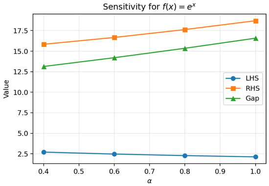
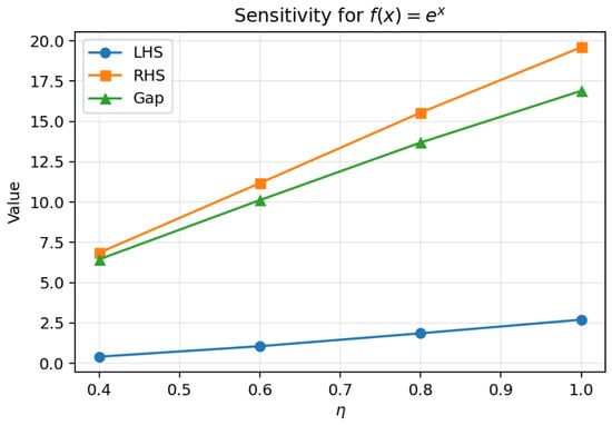
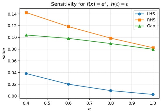
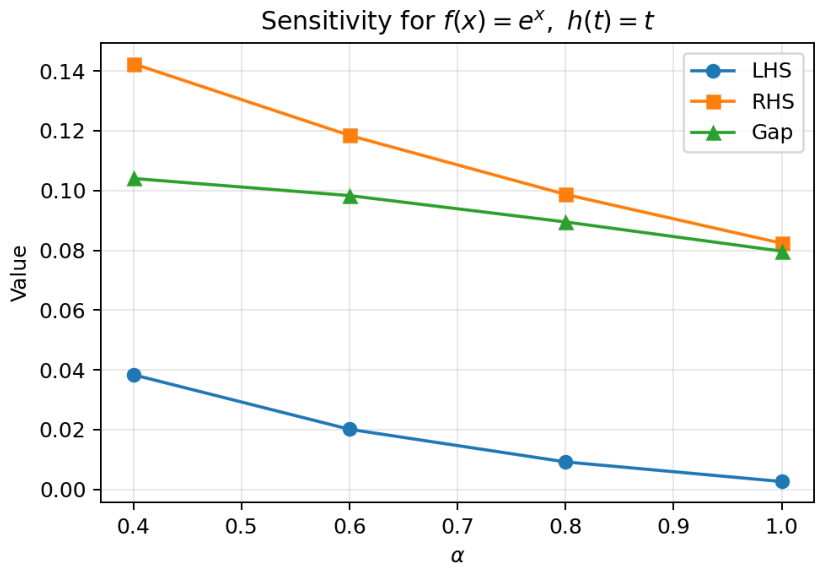
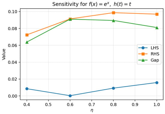
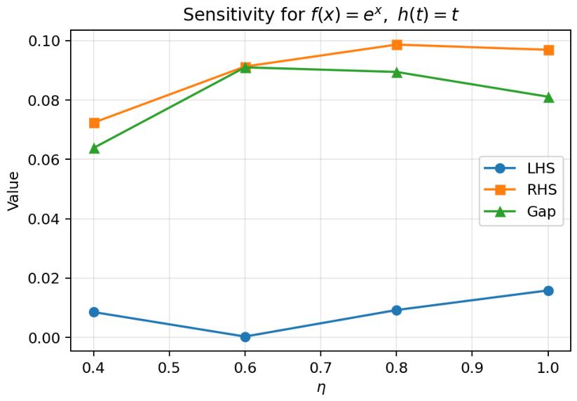
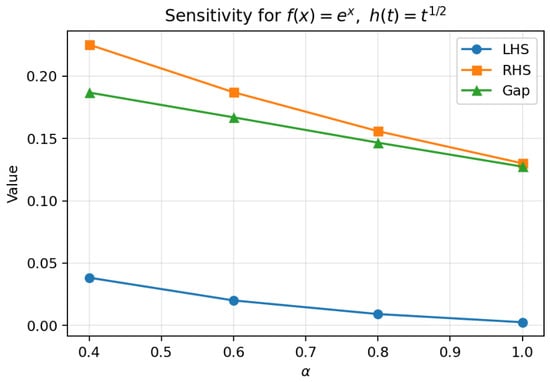
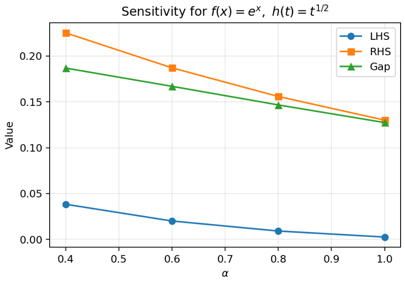
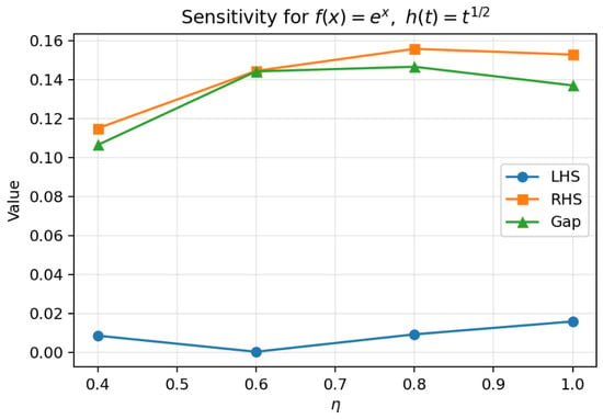
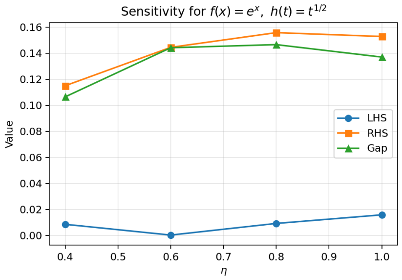
$h\left(t\right)=1$, and $B\left(\eta \right)=1$. Then $h\left(t\right)=1$ corresponds to the P-convex case. Table 2 and Figure 1 show the sensitivity with respect to $\alpha$ when $\eta =0.9$ is fixed. Table 3 and Figure 2 show the sensitivity with respect to $\eta$ when $\alpha =0.8$ is fixed.

Table 2. Gap sensitivity for Theorem 1 with $f\left(x\right)=e^x$, $h\left(t\right)=1$, and fixed $\eta =0.9$.

$\mathit{\alpha }$	LHS	RHS	Gap = RHS − LHS
0.4	2.705013	15.836448	13.131436
0.6	2.467191	16.667896	14.200705
0.8	2.279530	17.627033	15.347504
1.0	2.125261	18.703467	16.578206

Figure 1. Sensitivity of LHS, RHS, and Gap for $f\left(x\right)=e^x$, $h\left(t\right)=1$, and fixed $\eta =0.9$.

Table 3. Gap sensitivity for Theorem 1 with $f\left(x\right)=e^x$, $h\left(t\right)=1$, and fixed $\alpha =0.8$.

$\mathit{\eta }$	LHS	RHS	Gap = RHS − LHS
0.4	0.406360	6.848099	6.441739
0.6	1.055640	11.168180	10.112541
0.8	1.856272	15.539727	13.683455
1.0	2.701759	19.594768	16.893008

Figure 2. Sensitivity of LHS, RHS, and Gap for $f\left(x\right)=e^x$, $h\left(t\right)=1$, and fixed $\alpha =0.8$.

From Table 2 and Table 3, the inequality is valid for all displayed values of $\alpha$ and $\eta$ since the gap remains positive. When $\eta =0.9$ is fixed, among the tested values of $\alpha$, the smallest gap occurs at $\alpha =0.4$. When $\alpha =0.8$ is fixed, among the tested values of $\eta$, the smallest gap occurs at $\eta =0.4$. Thus, in this example, increasing either $\alpha$ or $\eta$ tends to enlarge the gap and produces a looser estimate.

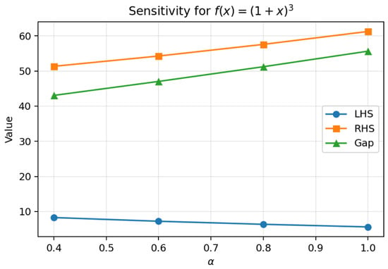
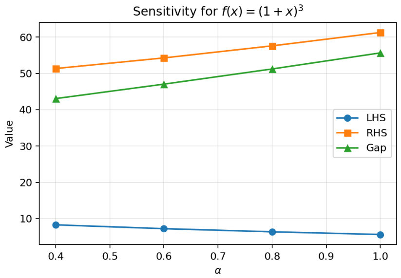
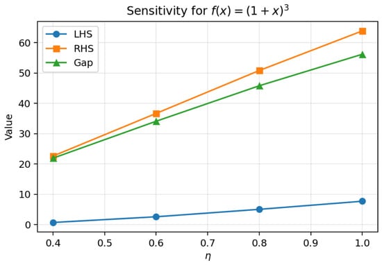
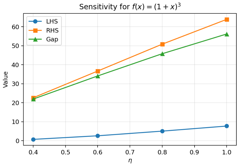
Numerical Example B. Let

$$f\left(x\right)={(1+x)}^3,[a,b]=[0,3],m=0.5,n=2,h\left(t\right)=1,B\left(\eta \right)=1.$$

Then $|f^{\prime }{\left(x\right)|=3(1+x)}^2$ is convex and non-negative on $[0,3]$; hence it is also P-convex. This example tests Theorem 1 for a polynomial function with a larger derivative magnitude.

The results in Table 4 and Table 5, together with Figure 3 and Figure 4, again confirm that Theorem 1 holds for all tested parameters. Compared with Example A, the gaps are larger because the derivative magnitude of ${(1+x)}^3$ on the relevant interval is larger than that of $e^x$. Among the tested parameter values of $\alpha$ and $\eta$, smaller values lead to smaller gaps, showing that these parameters act as sensitivity parameters in the numerical tightness of the estimate.

Table 4. Gap sensitivity for Theorem 1 with $f\left(x\right)={(1+x)}^3$, $h\left(t\right)=1$, and fixed $\eta =0.9$.

$\mathit{\alpha }$	LHS	RHS	Gap = RHS − LHS
0.4	8.284315	51.345262	43.060947
0.6	7.228487	54.271510	47.043023
0.8	6.361781	57.588609	51.226829
1.0	5.616920	61.273691	55.656772

Table 5. Gap sensitivity for Theorem 1 with $f\left(x\right)={(1+x)}^3$, $h\left(t\right)=1$, and fixed $\alpha =0.8$.

$\mathit{\eta }$	LHS	RHS	Gap = RHS − LHS
0.4	0.690623	22.616052	21.925429
0.6	2.577643	36.687868	34.110224
0.8	5.032182	50.849738	45.817556
1.0	7.705294	63.928013	56.222719

Figure 3. Sensitivity of LHS, RHS, and Gap for $f\left(x\right)={(1+x)}^3$, $h\left(t\right)=1$, and fixed $\eta =0.9$.

Figure 4. Sensitivity of LHS, RHS, and Gap for $f\left(x\right)={(1+x)}^3$, $h\left(t\right)=1$, and fixed $\alpha =0.8$.

Numerical Example C. Let

$$f\left(x\right)=e^x,a=0,b=1,m={\displaystyle \frac{1}{3}},n={\displaystyle \frac{2}{3}},$$

and choose $h\left(t\right)=t$. Since $h\left(t\right)=t$ corresponds to the classical convex case, Theorem 1 can be applied. For $\alpha =0.8$ and $\eta =0.8$, the left-hand side and right-hand side of Theorem 1 are computed as

$$\mathrm{LHS}=0.009218,\mathrm{RHS}=0.098689.$$

Hence $\mathrm{LHS}\le \mathrm{RHS}$, which verifies the validity of Theorem 1 in the convex setting. Table 6 and Table 7, together with Figure 5 and Figure 6, show the corresponding sensitivity with respect to $\alpha$ and $\eta$.

Table 6. Gap sensitivity for Theorem 1 with $f\left(x\right)=e^x$, $h\left(t\right)=t$, and fixed $\eta =0.8$.

$\mathit{\alpha }$	LHS	RHS	Gap = RHS − LHS
0.4	0.038385	0.142406	0.104021
0.6	0.020135	0.118426	0.098291
0.8	0.009218	0.098689	0.089471
1.0	0.002655	0.082354	0.079699

Table 7. Gap sensitivity for Theorem 1 with $f\left(x\right)=e^x$, $h\left(t\right)=t$, and fixed $\alpha =0.8$.

$\mathit{\eta }$	LHS	RHS	Gap = RHS − LHS
0.4	0.008538	0.072355	0.063817
0.6	0.000274	0.091296	0.091021
0.8	0.009218	0.098689	0.089471
1.0	0.015824	0.096941	0.081117

Figure 5. Sensitivity of LHS, RHS, and Gap for $f\left(x\right)=e^x$, $h\left(t\right)=t$, and fixed $\eta =0.8$.

Figure 6. Sensitivity of LHS, RHS, and Gap for $f\left(x\right)=e^x$, $h\left(t\right)=t$, and fixed $\alpha =0.8$.

Table 6 and Table 7 demonstrate that the convex case $h\left(t\right)=t$ also yields positive gaps for all tested parameter values. Hence the proposed inequality is not restricted to the P-convex choice $h\left(t\right)=1$.

Numerical Example D. Let

$$f\left(x\right)=e^x,a=0,b=1,m={\displaystyle \frac{1}{3}},n={\displaystyle \frac{2}{3}},$$

and choose $h\left(t\right)=t^{1/2}$. Then $h\left(t\right)=t^{1/2}$ represents a typical s-convex structure with $s=1/2$. For $\alpha =0.8$ and $\eta =0.8$, we obtain

$$\mathrm{LHS}=0.009218,\mathrm{RHS}=0.155814.$$

Therefore $\mathrm{LHS}\le \mathrm{RHS}$, confirming that Theorem 1 remains valid for s-convex functions. Table 8 and Table 9, together with Figure 7 and Figure 8, present the sensitivity with respect to $\alpha$ and $\eta$.

Table 8. Gap sensitivity for Theorem 1 with $f\left(x\right)=e^x$, $h\left(t\right)=t^{1/2}$, and fixed $\eta =0.8$.

$\mathit{\alpha }$	LHS	RHS	Gap = RHS − LHS
0.4	0.038385	0.225162	0.186777
0.6	0.020135	0.187036	0.166901
0.8	0.009218	0.155814	0.146597
1.0	0.002655	0.130042	0.127387

Table 9. Gap sensitivity for Theorem 1 with $f\left(x\right)=e^x$, $h\left(t\right)=t^{1/2}$, and fixed $\alpha =0.8$.

$\mathit{\eta }$	LHS	RHS	Gap = RHS − LHS
0.4	0.008538	0.115008	0.106470
0.6	0.000274	0.144494	0.144220
0.8	0.009218	0.155814	0.146597
1.0	0.015824	0.152845	0.137021

Figure 7. Sensitivity of LHS, RHS, and Gap for $f\left(x\right)=e^x$, $h\left(t\right)=t^{1/2}$, and fixed $\eta =0.8$.

Figure 8. Sensitivity of LHS, RHS, and Gap for $f\left(x\right)=e^x$, $h\left(t\right)=t^{1/2}$, and fixed $\alpha =0.8$.

The positive gaps in Table 8 and Table 9 confirm that the estimate remains valid in the s-convex case. Compared with the convex case $h\left(t\right)=t$, the weighting function $h\left(t\right)=t^{1/2}$ changes the size of the upper bound and therefore affects the numerical tightness of the inequality.

Discussion

Examples A–D demonstrate that the proposed inequalities remain applicable for several important subclasses of h-convex functions. In particular,

$$h\left(t\right)=1$$

corresponds to the P-convex case, and

$$h\left(t\right)=t$$

reduces to the classical convex case, while

$$h\left(t\right)=t^{1/2}$$

represents an s-convex structure. These examples illustrate that the obtained results are not restricted to a single convexity model and can be applied to a broad family of h-convex functions.

5. Conclusions

In this paper, we established new Milne–Mercer-type inequalities via Atangana–Baleanu conformable fractional integral operators for differentiable functions whose derivatives in absolute value are h-convex. A new identity associated with the ABConf fractional integral operator was first derived. By combining this identity with the Jensen–Mercer inequality and the h-convexity of $|f^{\prime }|$, we obtained new Milne–Mercer-type bounds.

The obtained results extend several known inequalities involving classical, Riemann–Liouville, conformable, and Atangana–Baleanu fractional integral operators. The special cases show that suitable choices of the parameters $\alpha$, $\eta$, and h recover familiar convex, P-convex, and s-convex forms. Therefore, the present approach provides a unified framework for treating Milne–Mercer-type inequalities in a broader fractional setting.

The numerical examples inserted between Theorems 1 and 2 provide a quantitative verification of the proposed estimate by using the gap $\mathrm{RHS}-\mathrm{LHS}$ as the main measure of tightness. For both $f\left(x\right)=e^x$ and $f\left(x\right)={(1+x)}^3$, the computed gaps are positive for all tested parameters, confirming the validity of Theorem 1. The tables and figures also show that the conformable and AB parameters influence the tightness of the inequality. In the tested cases, smaller displayed values of $\alpha$ and $\eta$ produce smaller gaps, whereas larger parameter values lead to looser upper bounds. Hence the additional parameters should be viewed as providing a flexible fractional framework, while the sharpness of the resulting estimate must be assessed through the gap rather than through the left-hand quantity alone.

The numerical examples inserted between Theorems 1 and 2 further reveal that the conformable parameter $\alpha$ and the fractional order $\eta$ play an important role in controlling the tightness of the obtained bounds. The sensitivity analysis shows that varying these parameters changes the size of the gap $\mathrm{RHS}-\mathrm{LHS}$, thereby influencing the effectiveness of the estimate. In particular, smaller tested values of $\alpha$ and $\eta$ generally lead to tighter bounds, whereas the limiting case $\alpha \to 1$ naturally recovers the corresponding Atangana–Baleanu fractional setting. These observations demonstrate that the ABConf framework not only unifies several existing fractional inequalities but also provides additional flexibility for adjusting the balance between fractional effects and numerical tightness.

Future research may investigate sharper versions of the present inequalities under stronger convexity assumptions, develop analogous results for other fractional operators, and apply the obtained bounds to numerical quadrature error estimates, approximation theory, and fractional differential equations.

References

- Atangana, A.; Baleanu, D. New fractional derivatives with non-local and non-singular kernel: Theory and applications to heat tranfer model. Therm. Sci. 2016, 20, 763–769. [Google Scholar]
- Atangana, A.; Koca, I. Chaos in a simple nonlinear system with Atangana-Baleanu derivative with fractional order. Chaos Solitons Fractals 2016, 89, 447–454. [Google Scholar]
- Butt, S.I.; Agarwal, P.; Neito, J.J. New Hadamard-Mercer Inequalities Pertaining Atangana-Baleanu Operator in Katugampola Sense with Application. Mediterr. J. Math. 2024, 21, 9. [Google Scholar] [CrossRef] [Scilit]
- Kermausuor, S.; Nwaeze, E.R. New fractional integral inequalities via k-Atangana-Baleanu fractional integral operators. Fractal Fract. 2023, 7, 740. [Google Scholar] [CrossRef] [Scilit]
- Set, E.; Akdemir, A.O.; Karaoĝlan, A.; Abdeljawad, T.; Shatanawi, W. On new generalizations of Hermite-Hadamard type inequalities via Atangana-Baleanu fractional integral operator. Axioms 2021, 10, 223. [Google Scholar] [CrossRef] [Scilit]
- Set, E.; Butt, S.I.; Akdemir, A.O.; Karaoglan, A.; Abdeljaward, T. New integral inequalities for differentiable convex functions via Atangana-Baleanu fractional integral operators. Chaos Solitons Fractals 2021, 143, 110554. [Google Scholar] [CrossRef] [Scilit]
- Butt, S.I.; Set, E.; Yousaf, S.; Abdeljawad, T.; Shatanawi, W. Generalized integral inequalities for ABK-fractional integral operators. AIMS Math. 2021, 6, 10164–10191. [Google Scholar] [CrossRef] [Scilit]
- Kashuri, A. Hermite-Hadamard type inequalities for the ABK-fractional intergals. J. Comput. Anal. Appl. 2021, 29, 309–326. [Google Scholar]
- Karim, M.; Fahmi, A.; Ullah, Z.; Bhatti, M.A.T.; Qayyum, A. On certain Ostrowski type integral inequalities for convex function via AB-fractional operator. AIMS Math. 2023, 8, 9166–9184. [Google Scholar] [CrossRef] [Scilit]
- Kermausuor, S.; Denu, D.; Olanipekun, P.O. ψ-Hilfer-Atangana-Baleanu fractional integral operators and some fractional integral inequaities. Kragujev. J. Math. 2026, 50, 1585–1604. [Google Scholar]
- Jiu, J.B.; Butt, S.I.; Nasir, J.; Aslam, A.; Fahad, A.; Soontharanon, J. Jensen-Mercer variant of Hermite-Hadamard type inequalities via Atangana-Baleanu fractional operator. AIMS Math. 2022, 7, 2123–2141. [Google Scholar] [CrossRef] [Scilit]
- Tariq, M.; Ahmad, H.; Sahoo, S.K.; Kashuri, A.; Nofal, T.A.; Hsu, C.H. Inequalities of Simpson-Mercer-type including Atangana-Baleanu fractional opeqrators and their applications. AIMS Math. 2022, 7, 15159–15181. [Google Scholar] [CrossRef] [Scilit]
- Tariq, M.; Ntouyas, S.K.; Ahmad, H.; Efendiev, R. Some new modifications of integral inequalities in the frame of AB fractional operator. Trans. Natl. Acad. Sci. Azerb. Ser. Phys.-Tech. Math. Sci. Math. 2026, 46, 1–22. [Google Scholar]
- Djenaoui, M.; Meftah, B. Milne type inequalities for differentiable s-convex functions. Honam Math. J. 2022, 44, 325–338. [Google Scholar]
- Çelik, B.; Budak, H.; Set, E. On generalized Milne type inequalities for new conformable fractional integrals. Filomat 2024, 38, 1807–1823. [Google Scholar] [CrossRef] [Scilit]
- Munir, A.; Qayyum, A.; Budak, H.; Faiz, I.; Kara, H.; Supadi, S.S. A study of Milne-type inequalities for several convex function classes with applications. Filomat 2024, 38, 11539–11551. [Google Scholar] [CrossRef] [Scilit]
- Mercer, A.M. A variant of Jensen’s inequality. J. Inequal. Pure Appl. Math. 2003, 4, 73. [Google Scholar]
- Benaissa, B.; Sarikaya, M.Z. Milne-Mercer type inequalities for h-convex functions. Filomat 2026, 40, 2393–2408. [Google Scholar] [CrossRef]
- Budak, H.; Kösem, P.; Kara, H. On new Milne-type inequalities for fractional integrals. J. Inequal. Appl. 2023, 2023, 10. [Google Scholar] [CrossRef] [Scilit]
- Jarad, F.; Ugurlu, E.; Abdeljawad, T.; Baleanu, D. On a new of fractional operators. Adv. Differ. Equ. 2017, 2017, 247. [Google Scholar] [CrossRef] [Scilit]
- Lo, J.C. Some Hermite-Hadamard-Mercer type inequalities via Atangana-Baleanu-Conformable fractional operator. AIMS Math. 2026, 11, 17937–17950. [Google Scholar]
Disclaimer/Publisher’s Note: The statements, opinions and data contained in all publications are solely those of the individual author(s) and contributor(s) and not of MDPI and/or the editor(s). MDPI and/or the editor(s) disclaim responsibility for any injury to people or property resulting from any ideas, methods, instructions or products referred to in the content. |
© 2026 by the author. Licensee MDPI, Basel, Switzerland. This article is an open access article distributed under the terms and conditions of the Creative Commons Attribution (CC BY) license.