


Abstract
The training of physics-informed neural networks (PINNs) for nonlinear multiphase flow in porous media is hampered by gradient conflicts between the individual components of the composite loss function. To address this problem, we propose a weighted gradient consistency metric that jointly accounts for the magnitudes and directions of the gradients of each loss term. Theoretical estimates of the convergence rate are derived, relating the proposed metric to the spectral properties of the preconditioner. The method is evaluated through a comparative study of optimizers—Adam, L-BFGS, and self-scaled Broyden—applied to three formulations of increasing complexity: a linear Buckley–Leverett model, a compressible two-phase model, and a fully nonlinear model with non-Newtonian rheology. The experiments demonstrate that self-scaled methods consistently achieve higher gradient alignment, faster loss reduction, and improved approximation accuracy compared to standard quasi-Newton and first-order baselines.
MSC:
76S05
1. Introduction
The modeling of a two-phase flow process with oil displacement from a porous medium, by water or its solutions of various consistencies, is one of the key tasks of the theory and practice of oil field development [1]. Maximum possible accuracy in the description of such processes is a necessary condition for an adequate forecast of production, the optimization of well operation modes, and evaluation of the effectiveness of increasing oil recovery methods [2,3]. Modern mathematical models of two-phase (even isothermal) flow, as a rule, are a system of nonlinear partial differential equations describing the mass and momentum conservation laws of phases, as well as closing semiempirical relations specifying the compressibility of reservoir fluids and rocks, phase permeability, capillary forces, and rheological laws. Except for simplified problem statements, the integration of a system of equations is possible only numerically. The classical approach is based on the application of spatial discretization based, for example, on finite element or finite volume methods; time approximation with an implicit or explicit Euler scheme; and linearization procedures such as Newton’s method [4]. Eventually, a system of algebraic equations with poor conditionality is formed, which significantly complicates its solution and challenges the convergence and adequacy of the numerical solution. This circumstance has led to the development of iterative sequential methods, the efficiency, stability, and convergence of which are largely determined by the chosen strategy of discretization of differential operators [5,6].
In recent years, the PINN approach [7], proposed as an alternative to classical numerical methods for solving partial differential equations, has attracted considerable interest. The PINN approach is based on the insertion of physically valid constraints directly into the neural network learning process, which makes it possible to eliminate explicit grid discretization and potentially simplify the solution of multidimensional and parametrically complex problems. In the context of describing flow problems, the PINN algorithm is considered a promising tool for accelerated modeling, building surrogate models, and solving inverse problems [8], including identifying reservoir and fluid parameters.
However, the application of PINNs to two-phase flow problems faces several additional difficulties in comparison with the description of the flow in a porous medium of a single-phase fluid [8]. PINN does not cope well with tasks with discontinuity in their solutions—for example, “saturation waves” [5] in the so-called Buckley–Leverett formulation, when the relative phase permeabilities (RFPs) are characterized by strong nonlinearity—which leads to coefficient degeneracy and a tight connection between the equations. These problems are significantly aggravated when the compressibility of all phases is considered, which leads to a deterioration in convergence during the neural network learning process.
The correct accounting of “non-Newtonian” rheology, even for a single oil phase, is particularly difficult. Experimental and field data [9] show that heavy and highly viscous oils exhibit nonlinear rheological behavior, which requires the use of more complex rheological models such as viscoplastic or pseudoplastic fluids. In addition, processes of sequential loading and unloading are accompanied by thixotropy, which involves changes in the internal structure of the oil. Non-Newtonian flow can be observed not only for highly viscous fluids but also for less viscous ones when moving in porous media with low porosity and permeability, as well as during special chemical reagent (polymers, gels) flow, which is applied in oil recovery enhancement technologies. Ignoring these properties during subsurface flow modeling can lead to significant errors in the forecasting of flow rates, the oil saturation of the reservoir, and the waterlogging of the products. Despite these findings, most of studies devoted to the problems of reservoir oil displacement, where the PINN approach is used, are limited to Newtonian rheology. This ultimately leads to an erroneous forecast of the values of the oil recovery coefficient and to an incorrect estimation of the effectiveness of the applied development technologies.
In [10], an extended XPINN approach is considered, designed to solve flow problems in highly inhomogeneous porous media. The method is based on the computing domain separation into homogeneous subdomains; a separate neural network is trained in each of them, and the interaction between the subdomains is provided through the interface conditions of pressure and flow continuity. Numerical experiments demonstrate the high accuracy of the obtained solutions; however, this approach requires preliminary domain partitioning and the simultaneous training of several neural networks, which significantly complicates its implementation and increases computational costs.
An alternative approach was proposed in [11], where generative adversarial networks integrated with physical constraints were applied to solve the Buckley–Leverett equation describing a two-phase flow in a porous medium. It was shown that this method effectively approximates the saturation front and has increased resistance to noisy data compared to classical PINN approaches. At the same time, the formulation under consideration was limited to a simplified model without considering the compressibility of phases and was based on Darcy’s linear law, which narrows the scope of the applicability of the results obtained.
In [12], a hybrid approach to solving the Burgers equation for a viscous medium is proposed, combining classical boundary layer theory (BLT) and modern physics-informed neural networks (PINNs). Boundary layer theory is applied to obtain an analytical approximation in areas where viscosity dominates (near boundaries), and PINNs are further trained to accurately reproduce nonlinear dynamics, including the formation of shock waves, in the entire solution domain.
In [13], a systematic analysis of the application of a PINN to the problem of two-phase flow, considering capillary pressure, was carried out within the framework of the Masket–Leverett model. The influence of the neural network’s architecture was researched, as was how the loss function’s shape and the placement strategy of the calculated points influenced method accuracy and stability. The results of numerical experiments show that the application of adaptive schemes that generate calculation points and modification of the loss function can improve the quality of approximation; however, the implementation of standard PINN algorithms still does not exclude problems during modeling problems of liquids of different viscosities and mobility saturation fronts’ propagation in a porous medium, which underlines the limitations of such a “classical approach” when solving more general problems of two-phase flow.
In recent years, PINN-related papers have payed more attention not only to the architecture of the neural network and the form of the loss function but also to the choice of optimization algorithm [14]. Several studies show that the learning task for PINNs differs significantly from standard machine learning tasks; the loss function, as a rule, consists of several terms that require satisfying equations, boundary and initial conditions, etc., which can be characterized by significantly different scales and have different “geometry” in the parameter space. As a result, a highly heterogeneous and poorly conditioned landscape of the loss function is formed, which leads to slow convergence, deceleration of the process up to a stop at local minimum points, and high sensitivity to the choice of hyperparameters of the optimizer [15].
In this paper, we investigate how the choice of optimization algorithm affects the quality and stability of PINN training for progressively more complex formulations of nonlinear two-phase flow problems in porous media, ranging from the classical Buckley–Leverett model to compressible and non-Newtonian flow regimes.
We introduce a weighted gradient consistency metric that quantifies the agreement between gradients of different loss components by considering both their directions and magnitudes. Unlike conventional gradient alignment measures based solely on cosine similarity, the proposed metric emphasizes the relative contribution of competing loss terms and enables analysis of optimization conflicts in stiff nonlinear PINN problems.
In contrast to adaptive loss balancing and optimizer adaptation strategies commonly used in the PINN literature [16], the proposed metric is not employed to modify the training process directly. Instead, it serves as a diagnostic and analytical tool for studying the geometry of the optimization landscape and the interaction between physical constraints during training.
In addition, we consider a self-scaled modification of the BFGS optimizer [17] that dynamically adjusts the parameter update step based on the local structure of the gradient field. A comparative study of standard and modified optimization algorithms has been conducted to evaluate convergence stability, gradient consistency, and approximation accuracy in the presence of saturation fronts and strong model nonlinearity.
2. Mathematical Statement
To describe the process of oil being displaced by water in a porous medium, we consider a one-dimensional unsteady two-phase flow model that accounts for phase compressibility and the non-Newtonian rheology of the displaced fluid.
The equations of phase continuity are defined as follows:
where corresponds to the water and oil phases accordingly; is the density of the phase; matrix porosity responds with m, the porosity coefficient; , the phase saturation; and , the flow rate of the corresponding phase .
Motion (flow) equations of each phase are set without considering capillary effects:
where k is the absolute permeability of the porous medium, is the relative phase permeability, is the dynamic viscosity of the phase, and p is the porous pressure.
The system is closed using the following relations, which account for the presence of two mobile phases in a deformable porous matrix, the dependence of oil viscosity on the pressure gradient, and the governing equations for weakly compressible phases:
where , , are the compressibility coefficients of the porous matrix, the water and oil phases, accordingly; , are the phase densities at porous pressure .
The nonlinearity of the flow process is due to the dependence of oil viscosity on the modulus of the pressure gradient , which reflects the transformation of the internal structure of the oil with a change in the intensity of the flow process. The parameter characterizes the viscosity of oil within an undisturbed structure, and —within a destroyed structure. Coefficient B determines the intensity of structural changes, and the parameter G sets the threshold value of the pressure gradient, above which the destruction of the structure begins.
The problem is defined over the following spatial domain and time interval:
The initial conditions assume uniform pressure and phase saturation throughout the domain, with water saturation set to the critical bound water value, while the boundary conditions represent injection at constant water pressure at the left boundary of the domain:
3. The Optimization Problem
Within the PINN approach, the solution of the two-phase flow problem is approximated by a parameterized function depending on the space–time coordinates. A neural network is considered as follows:
where is a set of trainable network parameters (a vector in the network parameter space , where d is the number of parameters to be trained), and the output components are the required pressure and water saturation fields.
This representation makes it possible to consider a neural network as an element of a finite-dimensional parametric subspace of the functional solution space. At the same time, the original problem of finding a continuous solution over the domain is reduced to a numerical optimization problem defined on a finite set of spatiotemporal points, including collocation points within the domain where the governing equations are enforced, as well as points where the initial and boundary conditions are satisfied.
A set of spatiotemporal points is defined as
Then the neural network approximation of the solution () with a set of trainable network parameters is defined as follows:
For other physical parameters of the problem, a similar representation will be applied.
3.1. Residual Pressure Equation
Substituting the neural network approximation expressions from (12) into the mass conservation Equation (1) and summing over both phases, the pressure discrepancy is determined as follows:
Here phase flow rates are determined as follows:
and the phase mobilities are determined as follows:
3.2. Residual Equation for Saturation
The residual for water saturation is determined from Equation (1) for the aqueous phase (w) as follows:
To increase the stability of PINN learning in the presence of saturation fronts (large saturation gradients) and the pronounced nonlinearity of the flow equations, we introduce an artificial viscosity with a constant coefficient. Adding an additional “diffusion” term makes it possible to smooth out numerical oscillations occurring in areas of large saturation gradients and provides a more stable approximation of the solution by a neural network. The coefficient of artificial viscosity is determined by a constant value and is assumed to be equal in all experiments: . The selection of the artificial viscosity parameter is discussed in Appendix A, where a sensitivity analysis based on RMSE and residual metrics is presented in Figure A1.
The constant artificial viscosity leads to a modified saturation equation containing an additional diffusion term with a coefficient .
which is used during formation of the loss function in the PINN algorithm. Numerical experiments show that the proposed modification significantly increases the stability of learning and makes it possible to reproduce saturation fronts correctly without the need for domain partitioning or the training of several neural networks.
3.3. Loss Function
The loss function is formed as a weight function considering the weight which corresponds to the i -term of the loss function (loss component)
where the contributions of the equation residuals (the first two terms), the residuals from the initial conditions (the third and fourth terms), and the residuals from the boundary conditions (the last two terms) are taken into account:
4. Gradient Consistency Metrics
To quantify the consistency of gradients across different components of the loss function, we introduce a gradient consistency metric. It considers not only the directions of the corresponding loss gradients, but also their modules, which makes it possible to more accurately assess the contribution of each loss component to the overall optimization direction, especially in the presence of sharp edges and local conflicts between the physical terms of the loss function.
The network loss function is represented as the sum of n components:
where corresponds to the equations residuals, boundary and initial conditions, or observational data. In the researched case . At the k-step of optimization, individual gradients are calculated with the neural network parameter of each component:
and the full gradient:
At a given iteration, the consistency metric is defined as the generalized cosine similarity between all pairs of gradients, taking into account their magnitudes.
Here and thereafter denotes the Euclidean norm in the parameter space of the network .
Parameter adjusts the sensitivity of the metric to gradient scale: at larger gradients get more weight, at smaller ones do. This makes it possible to adapt the metric to the specifics of the task. Within the framework of this paper, systematic study of the effect of was not conducted and is fixed in all experiments to ensure the simplicity and interpretability of the results obtained. This choice ensures that the weights are linearly dependent on the gradient norms.
values lie in the range :
- —large gradients are aligned (co-directional), and learning is effective;
- —the gradients are orthogonal on average, and the optimizer’s step is partially compensated;
- —large gradients counteract each other, and there is a conflict between the loss components.
Two types of estimations are set to analyze learning dynamics:
- Component consistency (intrastep), which evaluates the consistency of different components gradients in one iteration
- Full consistency (interstep) comparing the direction of the full gradient between neighboring iterations
The use of such metrics allows us to:
- Identify local conflicts between loss components that lead to learning delays;
- Evaluate the contribution of large and small (modulo) gradients, which is especially important for tasks with sharp saturation front;
- Compare the effectiveness of different optimizers (Adam, L-BFGS, self-scaled modifications);
- Quantify the dynamics of network convergence through gradient consistency indicators.
5. Theoretical Analysis of the Influence of Gradient Consistency
In this section, we formalize the relationship between the proposed gradient consistency metric and the rate of decrease of the loss function under conditional gradient descent. The loss function is considered as follows: where . is considered to be L-smooth relative to the Euclidean norm:
At each optimization step (iteration) k, preconditioned gradient descent with a preconditioning matrix and a learning rate are applied:
where the . matrix is considered to be symmetric and positively defined, and its spectrum is limited:
Values characterizing the spread of gradient norms are set:
The actual decrease in the loss function at the k-iteration is . Although the global loss landscape of a PINN is generally non-convex and may violate global L-smoothness, the optimization trajectories considered here originate from parameters obtained after a preliminary Adam phase. In this local region, the loss function typically exhibits a more regular, approximately quadratic behavior, making the L-smoothness assumption a reasonable local approximation. This is precisely the regime in which quasi-Newton methods (L-BFGS and the self-scaled Broyden method) operate, and thus the local analysis is directly relevant to the second stage of the training strategy. The assumption that the eigenvalues of lie within is consistent with standard BFGS-type approximations when combined with Wolfe line search and a positive definite initial Hessian. The self-scaled Broyden variant further reduces the ratio , effectively improving the conditioning of the inverse Hessian approximation.
Assumption 1
(about the lower limit of loss reduction). All the above assumptions are considered fulfilled, and the learning rate (η) satisfies the condition . Then the estimate is valid for any k:
where
Proof of Assumption 1.
Step 1
The standard inequality follows from the L-smoothness of the :
Substituting and transferring to the left, the inequality is obtained:
As and , where then
- Step 2: Evaluation of diagonal terms
Spectral decomposition is applied, as then is done for any vector x. Thus,
- Step 3: Evaluation of the cross terms
is defined. Then and then
Applying spectral estimates to results in and . Therefore,
Revealing the square of the norm of the original gradients sum,
where . Substituting the square of the norm in inequality (28), further obtains
- Step 4: The relation of the sum of pairwise intersections with the metric
It is noted that
, is defined. It was also defined that for each . Then
But as defined by metric. Therefore,
- Step 5: Evaluation of the last term in (26)
Similarly, with application of the inequality , it is obtained that
Applying the upper boundary from (30) for the sum of pairwise intersections, it is obtained that
- Final estimation
Terms (27), (29) (using the lower boundary from (30) for the cross terms) and (31) are substituted into (26):
□
5.1. Analysis of the Estimation Obtained
Let us consider the main factors influencing the value of the lower boundary.
- The coefficient A in the sum of the squares of the norms
This coefficient in inequality (24) is responsible for the contribution that does not depend on the consistency of the directions. It is quadratic relating to and reaches a maximum at
If (that is, the condition number ) then at any . In this case, the first term can slow down convergence, and a positive contribution can be obtained only at the cost of the second term at . A well-conditioned preconditioner ensures the positivity of A at small .
- Coefficient B for a weight metric
Coefficient B in inequality (24) determines how strongly the consistency of the gradients affects the loss reductions. The condition of B-positivity is provided by the condition
The multipliers and reflect the spread of gradient norms. With and the condition simplifies to . With the ratio can be less than one, which tightens the restriction on . Thus, a strong spread of norms () requires a more careful choice of steps to preserve the positive contribution of consistency.
Thus, the metric enables quantification of the relationship between gradient consistency and the efficiency of the optimization step, taking into account both the direction and magnitude of the gradients of each loss component. Under the additional assumption of the scalar of the preconditioner () and balanced norms the estimation (24) agreed with results in [18].
5.2. Two-Step Evaluation and Interstep Consistency
To complete the analysis, let us consider the effect of the step-by-step consistency of gradients on the total decrease in the loss function over two consecutive iterations. Let us define the interstep metric as the cosine of the angle between complete gradients at the nearest steps
Assumption 2
(On the two-step lower boundary). Let the assumptions introduced in the one-step evaluation be fulfilled. Then the estimate is valid for any two consecutive iterations
Proof of Assumption 2.
Step 1
By the definition of L-smoothness of the function , for any pair of vectors—in particular, for and —it holds that
Considering , and switching to the left, the following is obtained:
Let us evaluate the first linear term on the right side of the inequality (34). As , the following is obtained:
where the following condition is applied: .
- Step 2
To evaluate the second term on the right side consider as , then
As (the spectral norm of the difference does not exceed the difference between the maximum and minimum eigenvalues), the following is obtained:
Therefore, low estimation follows:
Thus,
Combining (35) with an estimate for , the following is obtained:
- Step 3
The estimation of the quadratic term in (34). With application of spectral boundaries:
and the triangle inequality, the following is obtained:
Substituting (36) and (37) into (34), the following inequality is obtained:
Grouping the terms, the required estimate is obtained (33). □
- Interpretation of the obtained estimate
Inequality (33) reveals the structure of the influence of interstep consistency on the dynamics of optimization. Let us consider separately the corresponding terms of inequality (33):
- Terms that depend only on the gradient norms:The first term reflects the potential contribution of the previous step, which can be positive for a sufficiently small ; the second term is always negative and is determined by the upper boundary of the norm of the preconditioned direction at the current step.
- Contribution of interstep consistency:This term is positive with and it becomes bigger as it approaches the gradient directions in neighboring iterations. Multiplier emphasizes that the effectiveness of consistency directly depends on the minimum eigenvalue of the preconditioner; a well-conditioned preconditioner enhances the positive effect.
- Negative cross term:This term is due to the spread of the preconditioner’s eigenvalues (the first term) and the quadratic approximation (the second term). The more poorly is conditioned (the more ), the higher the negative contribution of this term.
Thus, the total loss reduction in two steps is determined by the balance between the gains from gradient consistency and losses due to poor conditioning of the preconditioner. Well-designed optimizers (for example, self-scaled methods) tend to reduce , getting closer to the scalar matrix; this enhances the role of consistency and weakens negative terms. In the special case of a scalar preconditioner, the estimate (33) agrees with the results of [18].
5.3. Gradient and Quasi-Newton Methods
Consider the problem of minimizing a smooth loss function
First-order methods define an iterative process as follows:
where is the learning rate, which, in the general case, can change from iteration to iteration or adapt during the learning process (for example, in the Adam and RMSProp methods). These methods use only information about the gradient and do not consider the local curvature of the loss function. If the problem is poorly conditioned (a wide range of Hessian eigenvalues ), this leads to slower convergence and the appearance of oscillations along directions with high curvature. The second-order methods form an iterative process set as follows:
where is the Hessian of the loss function. For a quadratic local approximation of the loss function in one iteration (at ) the step is achieved by the exact minimum of this approximation. However, explicit calculation and inversion of the Hessian are computationally expensive in high-dimensional problems. Quasi-Newton methods accelerate gradient optimization by approximating the curvature of the loss function without explicitly calculating the Hessian. Instead of an exact matrix of second derivatives a sequence of matrices is constructed, approximating (Hessian itself), or —approximations of the inverse Hessian (as, for example, in the BFGS method, where the ). The matrix is updated recursively at each iteration, using only information about previous gradients and parameter changes, which makes it possible to consider the curvature of the landscape without explicitly reversing the Hessian and calculating the second derivatives. The Broyden set of methods is a general class of quasi-Newton algorithms in which a new approximation is obtained as a minimal change from the previous one , satisfying the secant condition from [19]. The obtained inverse Hessian approximation is applied as a precondition for the gradient, forming the direction of the step in the iterative process (40).
In the self-scaled modifications of the Broyden methods [17], an additional positive scaling of the inverse Hessian approximation is introduced. This scaling automatically corrects the overall level of curvature, reducing the impact of poor task conditioning. From a practical point of view, the self-scaled correction reconciles the accumulated quasi-Newton information with the current gradient changes, improving the stability of the search direction and the rate of convergence in problems with a significantly anisotropic landscape of the loss function.
In the context of the estimation, this leads to the following factors:
- Growth of the A-coefficient;
- An increase in the permissible range of , at which .
These theoretical conclusions are consistent with experimental observations, where self-scaled methods demonstrate faster and more stable convergence on stiff problems.
6. Examples of Computational Experiments
The solution of the same two-phase flow problem is now considered with a progressively more complex mathematical formulation. This approach makes it possible to trace how changes in the nonlinearity of the flow law and the stiffness of the system (phase compressibility) affect the dynamics of the optimization process and the evolution of the gradient consistency metric. Three levels of complexity of the two-phase flow model are considered:
- The first model is a linear formulation without considering the compressibility of the phases and with a constant viscosity for all phases, including oil (phase ), as in the classical Buckley–Leverett model (BL model);
- The second model, which considers the compressibility of the phases;
- The third model is a completely nonlinear model that includes both the equations of compressibility of the phases and the dependence of the viscosity of the displaced phase on the modulus of the pressure gradient.
This sequentially more complex formulation makes it possible to trace the influence of the system’s nonlinearity and stiffness on the optimization dynamics and the gradient consistency.
All numerical experiments assume the application of a fully connected neural network with eight hidden layers of 20 neurons each and a tanh activation function. The network approximates pressure fields and water saturation . Table A1 presents the parameters and their values used in the experiments.
The calculation options in the three formulations described above were compared between two neural network training strategies: (i) 1000 iterations of Adam followed by 200 iterations of L-BFGS; (ii) 400 iterations of Adam followed by 200 iterations of self-scaled Broyden.
This scheme reflects the common practice of first performing a first-order pre-training step, followed by refinement of the solution using quasi-Newton methods. For each case, we analyzed the dynamics of the loss function, intrastep gradient consistency , interstep consistency , the RMSE of the system of equations solution, and the stability of results across multiple runs.
The proposed analysis is complementary to existing PINN stabilization strategies for handling sharp fronts and discontinuities. A recent review [20] classifies such approaches into three main categories: (i) physics-based modifications, including artificial viscosity and entropy constraints; (ii) loss and training adaptations, such as adaptive weighting, causal loss formulations, and residual-based sampling; and (iii) architectural extensions, including domain decomposition methods (e.g., XPINNs), feature-enhanced networks, and kernel-based architectures such as KAN.
However, in our numerical experiments, the application of Fourier feature embeddings, causal loss formulations, adaptive artificial viscosity, residual-based sampling, and KAN-type architectures did not lead to a significant improvement in the accuracy of saturation front capturing. This observation is consistent with findings reported in [20], where many stabilization techniques demonstrate good performance for simplified formulations (e.g., the Buckley–Leverett equation), but their effectiveness deteriorates in fully coupled nonlinear systems involving multiple governing equations, where the approximation error increases significantly.
At the same time, we note that the combination of self-scaled quasi-Newton methods with the aforementioned stabilization techniques has not been explored in this study and remains an important direction for future research. In this work, we focus on analyzing the influence of optimization algorithms on training quality and stability.
6.1. First Formulation (Without Considering Compressibility and with Constant Phase Viscosity)
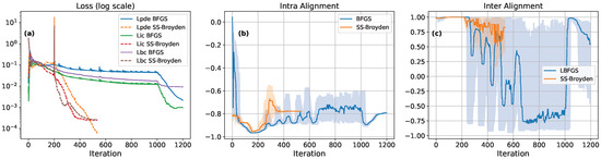
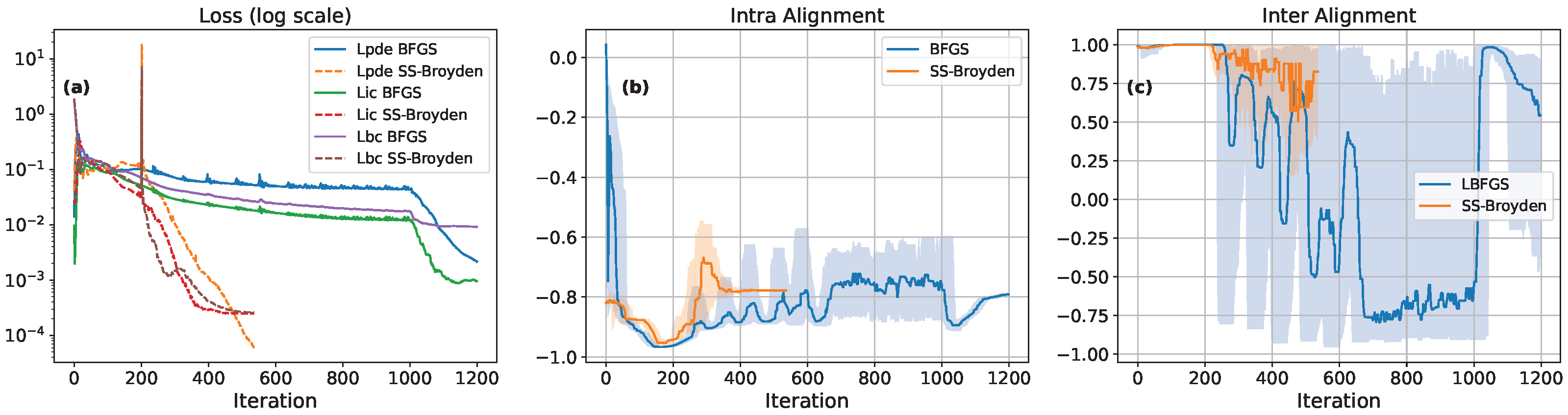
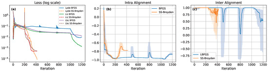
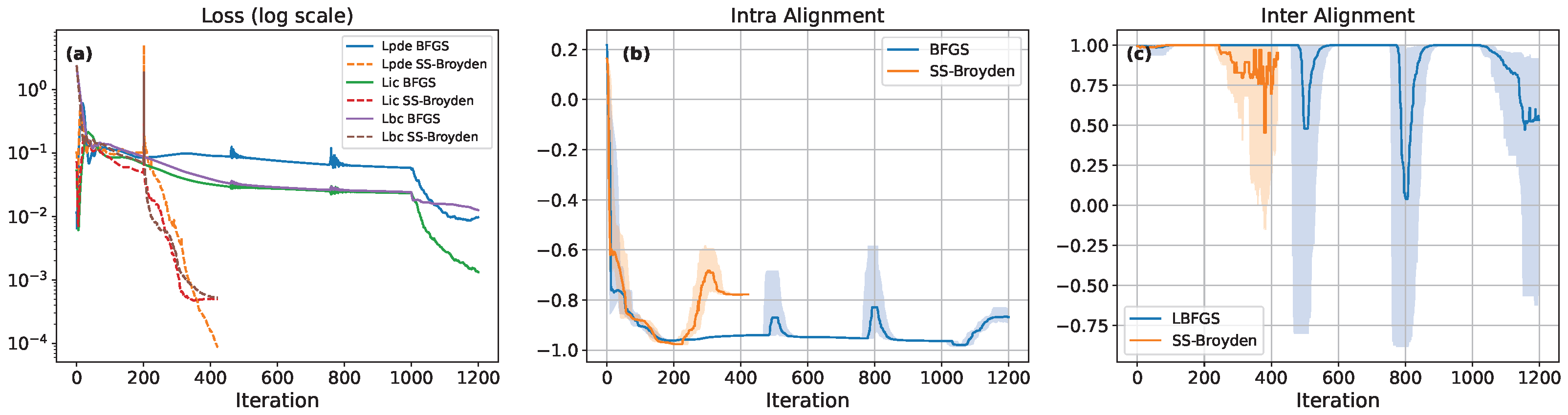
With application of the mathematical BL model, which assumes the constancy of densities and viscosities of the phases, the numerical solution is characterized by the dynamics of the loss function shown in the graphs in Figure 1 on the left (a) and demonstrating the degree of interstep and intrastep consistency ((b) and (c) of Figure 1, accordingly) when implementing the problem of minimizing the loss function using first-order method (39) and quasi-Newton methods (40). The dotted line on the (a) chart shows the change in the loss function during Adam + self-scaled Broyden optimization, and the solid lines show the change during Adam + LBFGS optimization.
Figure 1.
The dynamics of the loss function (a), intrastep consistency (b), and interstep consistency (c) for the formulation without considering compressibility and with constant viscosities of the phases.
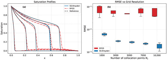
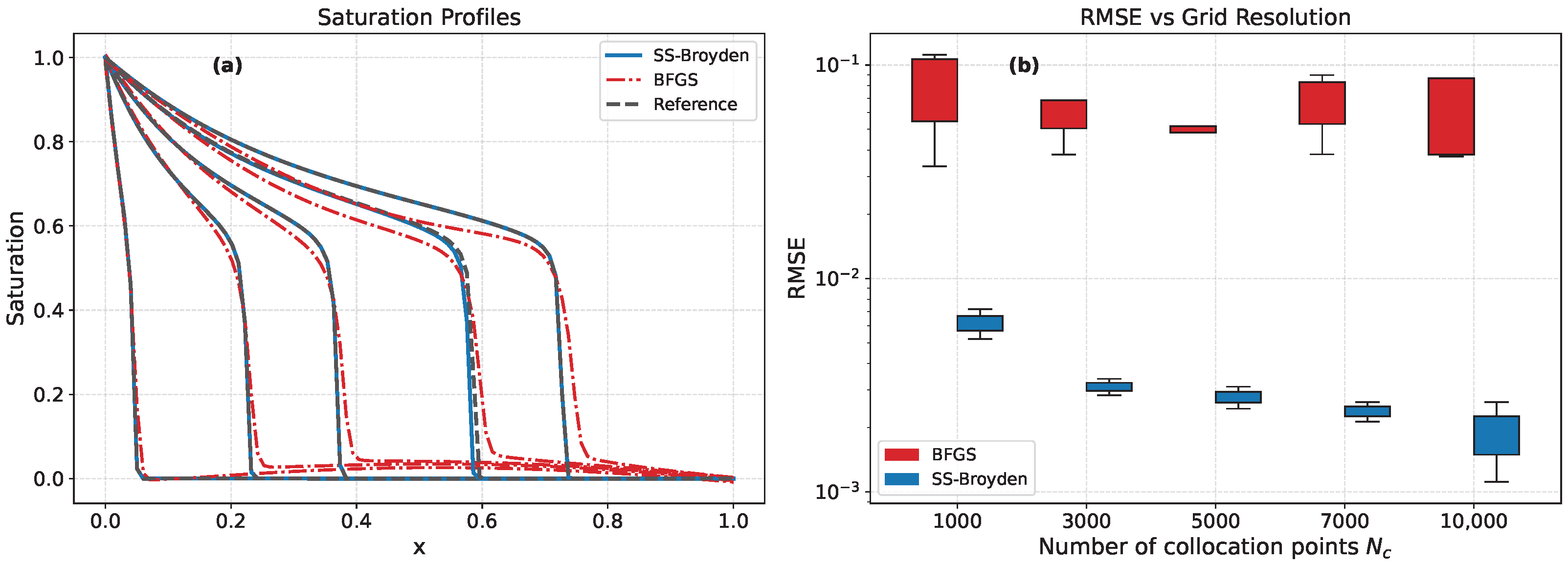
The (a) part of Figure 2 shows a comparison of saturation plots using the self-scaled Broyden and LBFGS optimization methods in comparison with the BL reference solution. The (b) side of Figure 2 shows the results of the RMSE depending on the grid resolution for linear formulation.
Figure 2.
(a) Comparison with the reference solution (dotted black line) of saturation plots with optimization with self-scaled Broyden (solid blue line) and LBFGS (dotted red line). Dependence of the approximation error (RMSE) on the grid resolution for linear formulation (b).
For the BL formulation, the dynamics of the loss function and consistency metrics (Figure 1) demonstrate a characteristic difference between the first-order and quasi-Newton methods. At the Adam learning stage, there is a slow decrease in the loss function and pronounced fluctuations in the interstep consistency of , which indicates an unstable optimization trajectory and alternating dominance of various loss components. The intrastep consistency quickly assumes values close to −1, which indicates a strong conflict between the gradient directions of individual components.
After switching to quasi-Newton methods, the dynamics of the optimization process stabilizes; the interstep consistency increases and remains close to 1, which reflects the alignment of the parameter update trajectory. The intrastep consistency remains negative, but its modulus decreases (values of the order of −0.8), which indicates a decrease in the degree of “conflict” between the various components (gradients) of the loss function.
The self-scaled modification demonstrates the smallest variation in and provides faster and deeper reduction of the loss function (by almost an order of magnitude compared to the classic L-BFGS approach), which confirms the effectiveness of automatic scaling in the presence of competing loss components.
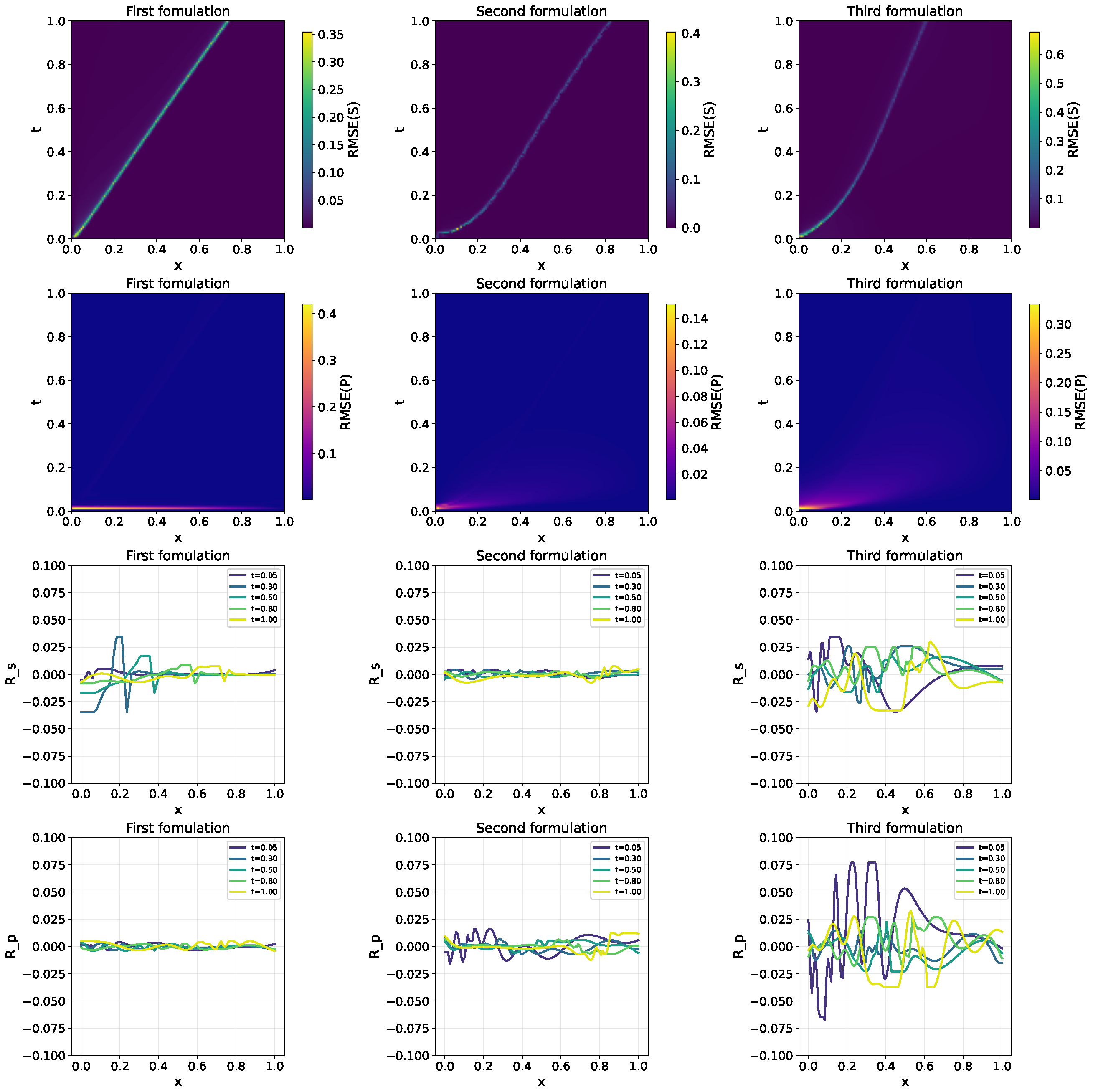
To clarify, in order to analyze the convergence over the space–time grid, the problem solution was restarted at least five times for each resolution, after which RMSE boxplot graphs were constructed (Figure 1). The solution obtained by the IMPES method with a spatial resolution of 100 cells and 3000 time steps was used as a reference. It is shown that the self-scaled modification demonstrates a faster decrease in error with increasing resolution and a significantly smaller spread of results, which indicates increased learning stability. The spatial distribution of the approximation error and PDE residuals are presented in Figure A2. The RMSE is largest near the saturation front while the residuals remain close to zero elsewhere, confirming that the PINN solution satisfies the governing equations with good fidelity.
6.2. Second Formulation (Considering Compressibility and with Constant Phase Viscosity)
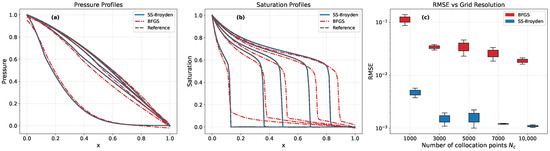
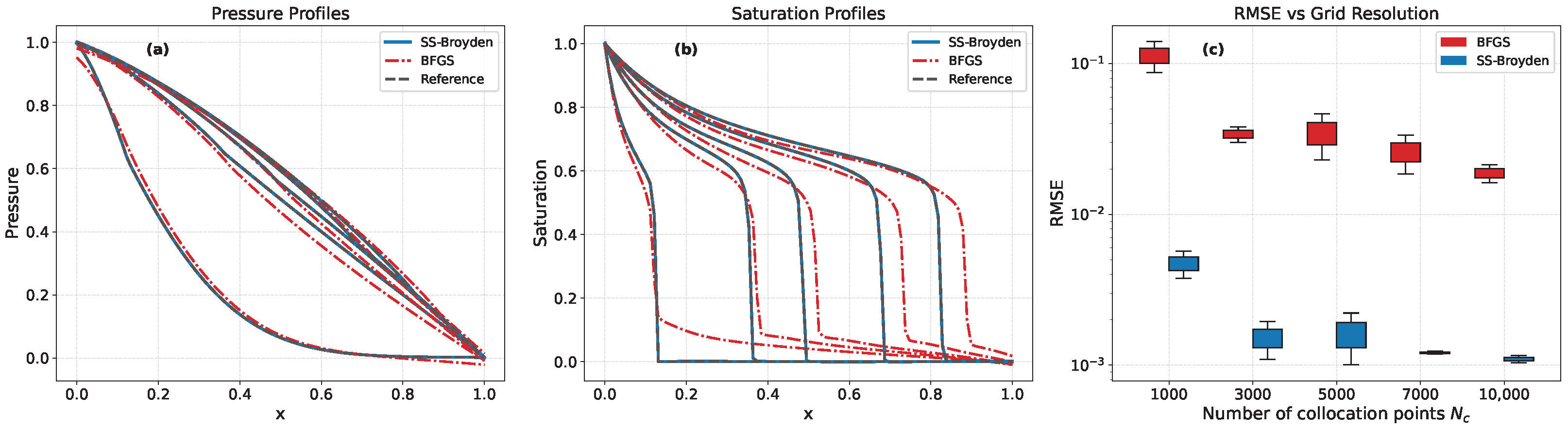
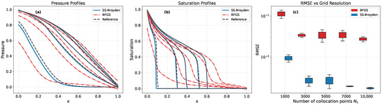
Figure 3 shows the dynamics of changes in the loss function considering the compressibility of phases (according to the model of a weakly compressible medium). The dynamics of consistency metrics differ from the linear formulation. The dotted line on the (a) chart shows the change in the loss function during Adam + self-scaled Broyden optimization, while the solid lines show the change during Adam + LBFGS optimization. As seen in Figure 4, which presents pressure plots (panel (a)) and graphs showing the progression of the saturation front (panel (b)), the flow hydrodynamics change significantly when accounting for the pressure dependence of phase densities. The RMSE representation (panel (c)) also varies depending on the grid resolution in the linear formulation.
Figure 3.
The dynamics of loss function (a), intrastep consistency (b) and interstep consistency (c) for the formulation considering compressibility and with constant viscosities of the phases.
Figure 4.
Comparison with the reference solution (dotted black line) of pressure diagrams (a) and saturation (b) when optimized with self-scaled Broyden (solid blue line) and LBFGS (dotted red line). Graph (c) shows the dependence of the approximation error (RMSE) on the grid resolution for linear formulation, considering the compressibility of the phases.
The solution of the optimization problem becomes more structurally consistent: when training with the Adam method, the intrastep consistency remains closer to −1, however, the spread of values almost disappears, indicating that the “conflict” has been stabilized between the loss components. At the same time, the interstep consistency of remains close to 1 throughout the training, reflecting a steady trajectory of parameter updates.
The transition to quasi-Newton methods leads to a moderate improvement in the intrastep consistency of , but is accompanied by a slight decrease in the interstep consistency of compared to Adam. The self-scaled modification demonstrates a more pronounced improvement in intrastep consistency and less degradation of interstep consistency (values stabilize around 0.8), providing the most balanced dynamics.
The behavior of the loss function qualitatively repeats the BL formulation; the self-scaled strategy provides the deepest reduction in loss with stable convergence.
6.3. The Third Formulation (Considering the Compressibility of the Phases and the Nonlinear Change in the Viscosity of the Displaced Phase)
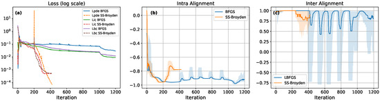
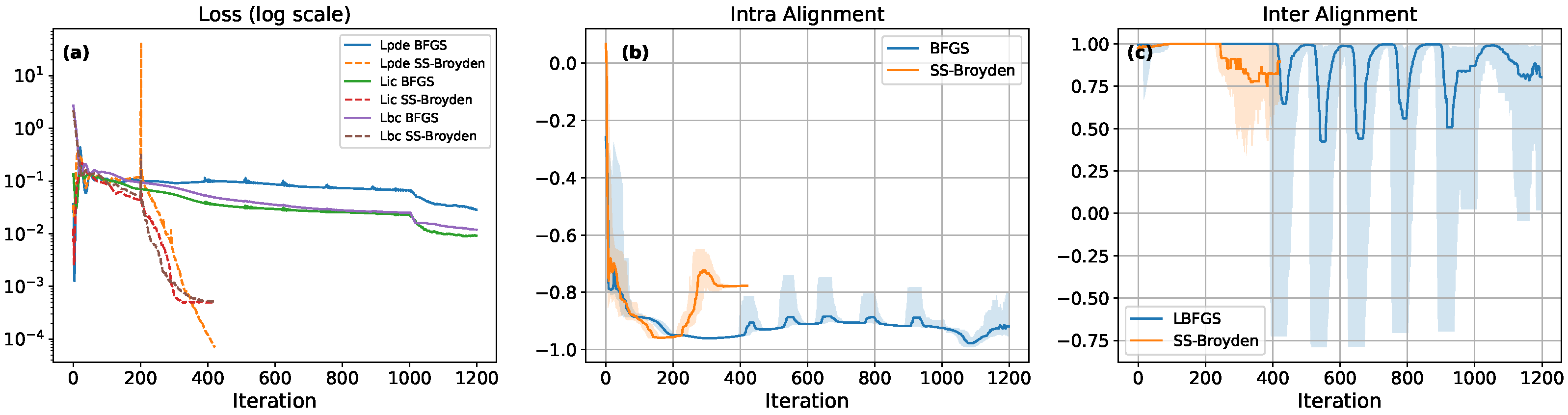
In the fully nonlinear formulation, where both the phase densities and the viscosity of the oil phase () vary with pressure, the characteristics of the numerical solution are illustrated in Figure 5 and Figure 6. These figures clearly show an increase in effects associated with the stiffness of the system.
Figure 5.
The dynamics of the loss function (a), intrastep consistency (b) and interstep consistency (c) for the formulation considering compressibility and with a nonlinear law of viscosity change. The dotted line on the left graph is the change in the loss function during optimization with Adam + self-scaled Broyden. The solid lines are for Adam + LBFGS.
Figure 6.
Comparison with the reference solution (dotted black line) of pressure (a) and saturation (b) plots when optimized with self-scaled Broyden (solid blue line) and LBFGS (dotted red line). The dependence of the approximation error (RMSE) on the resolution of the grid for formulation, taking into account the compressibility of phases and the nonlinear law of viscosity variation (c).
Intrastep consistency in Adam training is again characterized by values close to the value of , which indicates an increase in the multidirectional influence of the components of the loss function. In contrast to the previous case (considering only compressibility), there remains a noticeable variability in intrastep consistency function , reflecting the increased sensitivity of the iterative process to local changes in pressure and saturation. At the same time, the interstep consistency of with Adam shows more pronounced fluctuations compared to previous formulations, which indicates the instability of the optimization trajectory in conditions of strong nonlinearity.
Quasi-Newton methods partially compensate for this effect; the function is characterized in terms of negative values somewhat closer to the level, and on the contrary, stabilizes at a higher level, although periodic drawdowns associated with local rearrangements of the approximation process are occurred.
The self-scaled modification ensures the most stable behavior of control functions: intra–step consistency improves more significantly, and interstep consistency remains at the level of 0.8–0.9 with a smaller spread compared to the standard L-BFGS variant.
The dynamics of the loss function retains the qualitative structure observed in previous experiments; the self-scaled strategy provides the deepest reduction in loss. At the same time, the absolute approximation error increases in comparison with linear cases, which is naturally caused by the increased nonlinearity of the model. Thus, a stable pattern is observed in all three formulations, considering the curvature of the loss function increases the intrastep consistency of gradients and stabilizes the interstep dynamics, which directly affects the speed and stability of the loss function reduction. The self-scaled modification further improves the balance between loss components, providing more stable and predictable optimization, especially in nonlinear tasks.
6.4. Computational Cost Considerations
A preliminary assessment of the computational cost is provided below, while a systematic comparison with classical solvers across a wider range of problem sizes is deferred to future work. In the present experiments, the complete training schedule (1000 Adam iterations followed by 200 BFGS iterations) requires approximately 10 min on a single GPU, while the reduced schedule (400 Adam + 200 Broyden iterations) completes in about 6 min. We acknowledge that this is longer than a single run of the IMPES reference solver on the same spatiotemporal grid.
The practical advantage of the PINN approach, however, becomes apparent when pre-trained models are reused. As demonstrated in recent work [21], a pre-trained PINN can serve as a computational cache for related problem settings. When training starts from a pre-trained state and an early-stopping criterion (e.g., five consecutive iterations without loss improvement) is applied, the fine-tuning time drops to approximately 30 s, which is comparable to or even faster than a conventional IMPES solve. Moreover, unlike IMPES, the PINN solution is less sensitive to grid resolution.
7. Conclusions
The paper examines the role of gradient consistency in PINN training for two-phase flow problems in porous media under various task formulations. The proposed interpretation of intrastep and interstep consistency metrics made it possible to link the geometry of the gradient structure of the loss function with the dynamics of optimization and learning stability.
Theoretical analysis has shown that considering the curvature of the loss function through conditional steps reduces the “conflict” between the loss components and stabilizes the trajectory of parameter updates. Numerical experiments for linear, compressible, and fully nonlinear formulations have confirmed this hypothesis; quasi-Newton methods demonstrate higher intrastep consistency, more stable interstep dynamics, and a deeper reduction in the loss function compared to Adam. Self-scaled modifications provide additional improvements by automatically scaling the gradient components.
It is shown that, as the nonlinearity of the model increases, the benefits of methods that account for curvature become more pronounced. This is particularly important for applied oil and gas modeling problems, where stiffness and physical realism—including the nonlinearity of phase properties—are typical features of the mathematical formulation. These factors significantly affect the accuracy of numerical solutions in representing the real characteristics of the development process.
It is worth noting that using the PIKAN architecture in the tasks considered did not lead to a noticeable improvement in approximation accuracy. This suggests that under conditions of strong “competition” (multidirectionality) among the components of the loss function, the key factor for solution quality is not the network architecture itself, but rather the choice and configuration of the optimization algorithm.
As a direction for further research, it seems promising to study methods based on the Newton–Krylov approaches, which make it possible to more fully consider the Hessian structure when solving highly nonlinear problems. An analysis of their impact on consistency metrics and the stability of PINN learning can provide additional insight into the role of high-precision quasi-Newtonian and Newtonian schemes in flow problems with expressed nonlinearity.
Author Contributions
Conceptualization, M.K. and D.A.; methodology, M.K., D.A. and N.S.; software, D.A.; validation, M.K. and D.A.; writing—original draft preparation, M.K., D.A. and N.S.; writing—review and editing, M.K. and N.S.; visualization, D.A.; supervision, N.S. All authors have read and agreed to the published version of the manuscript.
Funding
The work was supported by the Ministry of Education and Science of the Russian Federation as part of the program of the Moscow Center for Fundamental and Applied Mathematics under the Agreement No. 075-15-2025-345.
Data Availability Statement
Data and source code of the experiments are available at the GitHub repository (https://github.com/aminevdam/2phase_nonlinear_PINN, accessed on 2 April 2026).
Acknowledgments
The work was supported by the Ministry of Education and Science of the Russian Federation as part of the program of the Moscow Center for Fundamental and Applied Mathematics under the Agreement No. 075-15-2025-345. The study was conducted under the state assignment of Lomonosov Moscow State University.
Conflicts of Interest
The authors declare no conflicts of interest. The funders had no role in the design of the study; in the collection, analyses, or interpretation of data; in the writing of the manuscript; or in the decision to publish the results.
Nomenclature
| gradient of the i-th loss component at iteration k | |
| k | absolute permeability of the porous medium |
| relative phase permeability of phase | |
| m | porosity |
| p | pore pressure |
| preconditioning matrix at iteration k | |
| residual of the pressure equation | |
| residual of the saturation equation (without artificial viscosity) | |
| residual of the saturation equation (with artificial viscosity) | |
| saturation of phase | |
| neural network approximation of water saturation | |
| neural network approximation of pore pressure | |
| volumetric flow rate of phase | |
| exponent controlling sensitivity of the consistency metric | |
| decrease of the loss function at iteration k | |
| learning rate | |
| vector of trainable neural network parameters | |
| mobility of phase | |
| dynamic viscosity of phase | |
| artificial viscosity coefficient | |
| lower and upper bounds of the preconditioner spectrum | |
| density of phase | |
| weighted gradient consistency metric | |
| intrastep gradient consistency | |
| interstep gradient consistency | |
| IMPES | implicit pressure, explicit saturation |
| PDE | partial differential equation |
| PINN | physics-informed neural network |
| RMSE | root mean square error |
Appendix A
In PINN-based approximations, the use of smooth activation functions such as the hyperbolic tangent implies that the neural network represents a continuous function. However, the target solution in multiphase flow problems typically exhibits sharp fronts and discontinuities, which are difficult to approximate directly within this framework.
To address this issue, we introduce an artificial viscosity term that smooths the solution and improves training stability. This approach is consistent with recent studies [20], where it is shown that adding artificial diffusion enhances convergence and enables more accurate front capturing in PINNs. To determine an appropriate value of the artificial viscosity coefficient, a series of numerical experiments was conducted for the first formulation (BL) problem using different viscosity values. For each configuration, the RMSE, the residuals (from (15)) and (from (13)) were evaluated. The results of this sensitivity study are presented in Figure A1. Based on these results, the value was selected as a compromise between approximation accuracy and residual minimization. For consistency, this value of artificial viscosity was used in all subsequent experiments presented in the paper.
Figure A1.
Sensitivity analysis for the artificial viscosity coefficient in the linear Buckley–Leverett formulation. (a) Distribution of the PDE residuals (pressure equation) and (saturation equation, orange) over the collocation points for different values of . (b) RMSE between the PINN solution and the reference IMPES solution at different values.
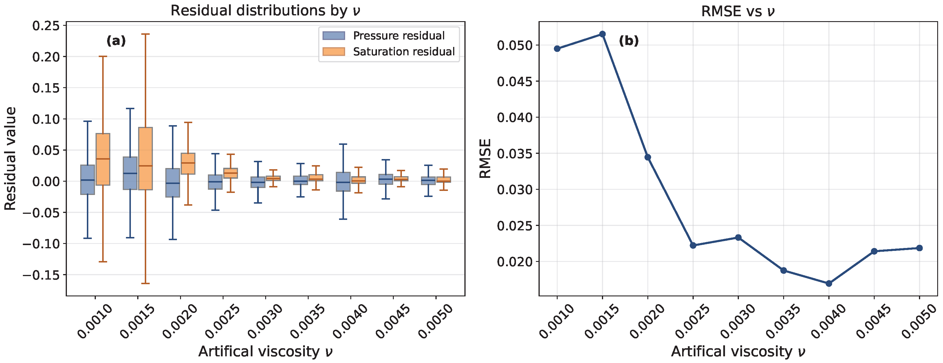
Figure A2 shows the space–time distributions of the pointwise RMSE and PDE residuals for all three formulations. The error remains concentrated near the saturation front, while the residuals are tightly clustered around zero throughout the computational domain.
Figure A2.
Space–time heat maps of the approximation error and PDE residuals for all three model formulations. Rows 1 and 2: pointwise RMSE for water saturation and pressure p, respectively. Rows 3 and 4: absolute values of the saturation residual and the pressure residual . Columns correspond to the linear Buckley–Leverett formulation (left), the compressible formulation (centre), and the fully nonlinear formulation (right). All results are shown for the self-scaled Broyden optimizer at the final training iteration.
The parameters used in all numerical experiments are listed in Table A1.
Table A1.
Modelling parameters.
References
- Dake, L.P. The Practice of Reservoir Engineering (Revised Edition); Elsevier: Amsterdam, The Netherlands, 2001; Volume 36. [Google Scholar]
- Dieva, N.; Kravchenko, M.; Afanaskin, I.; Arhipov, A.; Pivovarov, D. Mathematical model with nonlinear dependence of porosity and permeability on pressure at reservoir pressure below bubble point pressure for analysis of oil fields development in depletion mode (Russian). Oil Ind. J. 2024, 2024, 98–102. [Google Scholar] [CrossRef] [Scilit]
- Afanasyev, A.; Andreeva, A.; Chernova, A. Influence of oil field production life on optimal CO2 flooding strategies: Insight from the microscopic displacement efficiency. J. Pet. Sci. Eng. 2021, 205, 108803. [Google Scholar] [CrossRef] [Scilit]
- Samarsky, A.; Gulin, A. Numerical Methods; Nauka: Moscow, Russia, 1989. [Google Scholar]
- Barenblatt, G.I.; Yentov, V.M.; Ryzhik, V.M. Theory of Nonstationary Liquid and Gas Filtration; Nedra: Moscow, Russia, 1972. [Google Scholar]
- Garipov, T.T.; Tomin, P.; Rin, R.; Voskov, D.V.; Tchelepi, H.A. Unified thermo-compositional-mechanical framework for reservoir simulation. Comput. Geosci. 2018, 22, 1039–1057. [Google Scholar] [CrossRef] [Scilit]
- Raissi, M.; Perdikaris, P.; Karniadakis, G.E. Physics-informed neural networks: A deep learning framework for solving forward and inverse problems involving nonlinear partial differential equations. J. Comput. Phys. 2019, 378, 686–707. [Google Scholar] [CrossRef] [Scilit]
- Dieva, N.; Aminev, D.; Kravchenko, M.; Smirnov, N. Overview of the application of physically informed neural networks to the problems of nonlinear fluid flow in porous media. Computation 2024, 12, 69. [Google Scholar] [CrossRef] [Scilit]
- Baikov, V.; Kolonskih, A. Method for Determining Stagnant and Poorly Drained Oil Zones in Low-Permeability Reservoirs. Available online: https://rusneb.ru/catalog/000224_000128_0002524719_20140810_C1_RU/ (accessed on 2 May 2026).
- Alhubail, A.; He, X.; AlSinan, M.; Kwak, H.; Hoteit, H. Extended physics-informed neural networks for solving fluid flow problems in highly heterogeneous media. In Proceedings of the International Petroleum Technology Conference (IPTC), Riyadh, Saudi Arabia, 21–23 February 2022; p. D031S073R001. [Google Scholar]
- Ma, X.; Li, C.; Zhan, J.; Zhuang, Y. Physics-Informed Generative Adversarial Network Solution to Buckley–Leverett Equation. Mathematics 2024, 12, 3833. [Google Scholar] [CrossRef] [Scilit]
- Ortiz Ortiz, R.D.; Martínez Núñez, O.; Marín Ramírez, A.M. Solving Viscous Burgers’ Equation: Hybrid Approach Combining Boundary Layer Theory and Physics-Informed Neural Networks. Mathematics 2024, 12, 3430. [Google Scholar] [CrossRef] [Scilit]
- Imankulov, T.; Kuljabekov, A.; Bekele, S.D.; Zhantayev, Z.; Assilbekov, B.; Kenzhebek, Y. A Systematic Analysis of Physics-Informed Neural Networks for Two-Phase Flow with Capillarity: The Muskat–Leverett Problem. Appl. Sci. 2025, 15, 13011. [Google Scholar] [CrossRef] [Scilit]
- Müller, J.; Zeinhofer, M. Achieving high accuracy with PINNs via energy natural gradient descent. In Proceedings of the International Conference on Machine Learning, PMLR 2023, Honolulu, HI, USA, 23–29 July 2023; pp. 25471–25485. [Google Scholar]
- Rathore, P.; Lei, W.; Frangella, Z.; Lu, L.; Udell, M. Challenges in training pinns: A loss landscape perspective. arXiv 2024, arXiv:2402.01868. [Google Scholar] [CrossRef] [Scilit]
- Wang, S.; Yu, X.; Perdikaris, P. When and why PINNs fail to train: A neural tangent kernel perspective. J. Comput. Phys. 2022, 449, 110768. [Google Scholar] [CrossRef] [Scilit]
- Kiyani, E.; Shukla, K.; Urbán, J.F.; Darbon, J.; Karniadakis, G.E. Optimizing the optimizer for physics-informed neural networks and Kolmogorov-Arnold networks. Comput. Methods Appl. Mech. Eng. 2025, 446, 118308. [Google Scholar] [CrossRef] [Scilit]
- Wang, S.; Bhartari, A.K.; Li, B.; Perdikaris, P. Gradient alignment in physics-informed neural networks: A second-order optimization perspective. arXiv 2025, arXiv:2502.00604. [Google Scholar]
- Broyden, C.G. Quasi-Newton methods and their application to function minimisation. Math. Comput. 1967, 21, 368–381. [Google Scholar] [CrossRef]
- Abbasi, J.; Jagtap, A.D.; Moseley, B.; Hiorth, A.; Andersen, P.Ø. Challenges and advancements in modeling shock fronts with physics-informed neural networks: A review and benchmarking study. arXiv 2025, arXiv:2503.17379. [Google Scholar] [CrossRef] [Scilit]
- Hvatov, A. Automated Differential Equation Solver Based on the Parametric Approximation Optimization. Mathematics 2023, 11, 1787. [Google Scholar] [CrossRef] [Scilit]
Disclaimer/Publisher’s Note: The statements, opinions and data contained in all publications are solely those of the individual author(s) and contributor(s) and not of MDPI and/or the editor(s). MDPI and/or the editor(s) disclaim responsibility for any injury to people or property resulting from any ideas, methods, instructions or products referred to in the content. |
© 2026 by the authors. Licensee MDPI, Basel, Switzerland. This article is an open access article distributed under the terms and conditions of the Creative Commons Attribution (CC BY) license.