


Abstract
Monkeypox (Mpox), a zoonotic Orthopoxvirus disease, was declared a Public Health Emergency of International Concern by the WHO in 2022. While the global fatality rate is approximately 0.7%, mortality risks vary significantly across regions and remain high for vulnerable groups, necessitating precise predictive models for public health resource allocation. This study proposes TRAGIC, a novel fusion model integrating Transformer, GRU, and Quick Attention mechanisms to predict monkeypox death cases. Utilizing a global dataset with a comprehensive set of 16 input features, the TRAGIC model was benchmarked against traditional GRU, LSTM, Transformer, and Trans-GRU architectures. Experimental results demonstrate that TRAGIC consistently outperforms existing deep learning models, particularly in capturing non-linear patterns and long-term dependencies in epidemic time-series data. The findings suggest that the TRAGIC model offers superior accuracy and stability, providing a robust tool for forecasting infectious disease mortality and supporting global health policymaking.
Keywords:
mpox mortality prediction; time-series forecasting; TRAGIC fusion model; gated recurrent unit (GRU); Quick Attention; Explainable AI (XAI) MSC:
92D30; 62M10; 68T07; 62P10
1. Introduction
When emerging infectious diseases pose a significant threat to global health security, they demand urgent and coordinated attention from the international scientific community. Among these, Monkeypox (Mpox) has emerged as a primary concern due to its potential for cross-species transmission and rapid international spread. The monkeypox virus is primarily transmitted between humans through respiratory secretions during prolonged face-to-face interactions, as well as through sexual contact with the bodily fluids of infected individuals [1,2]. The virus enters the human body via open wounds (even if not visible), respiratory mucous membranes, or the eyes, nose, and mouth. The incubation period typically ranges from 7 to 14 days, though it can span from 5 to 21 days; symptoms generally persist for 2 to 4 weeks. Historically, the case fatality rate among patients has ranged from 0% to 11% [3].
Predicting monkeypox mortality is crucial for global public health, as it enables the timely implementation of containment measures and the strategic allocation of resources. According to the World Health Organization (WHO), by October 2022, the monkeypox outbreak had rapidly spread to more than 100 countries, resulting in 136 deaths worldwide. Despite a low overall mortality rate, risk is disproportionately elevated among vulnerable populations, particularly pediatric and immunocompromised individuals. Mortality figures serve as a vital indicator of outbreak severity, helping governments and health agencies identify high-risk epicenters, formulate targeted interventions, and optimize the distribution of vaccines and medical supplies. However, traditional predictive models often exhibit bias due to the struggles of capturing the nonlinear and volatile dynamics characteristic of modern epidemics [4].
To improve forecasting accuracy, scholars have explored advanced computational techniques. Dada et al. [4] utilized Stacking Ensemble Learning (SEL) to combine multiple base models. While SEL can enhance predictive performance, that specific study selected only 3 out of 18 monkeypox-related symptoms as input variables. This limited scope may fail to comprehensively capture the complexities of the disease, leading to suboptimal performance. Similarly, Iftikhar et al. [5] proposed a hybrid deep learning method based on the Al-Biruni Earth Radius (BER) optimization technique to tune the hyperparameters of Long Short-Term Memory (LSTM) models. Despite these advancements, the diverse and complex nature of Mpox symptoms means that models relying on a narrow set of variables cannot fully account for all factors influencing transmission and clinical outcomes.
Time series analysis remains a powerful tool for identifying cycles, seasonal patterns, and recurring trends in epidemic data [6]. However, most current studies rely on single-model time series approaches. These models frequently encounter limitations when faced with complex data and regional variations [4]. Furthermore, traditional models often produce delayed results when dealing with rapidly evolving outbreaks due to data latency, and fixed-interval time series often struggle to accurately reflect the true dynamics of disease transmission [7].
To address these limitations, this study explores the potential of multi-model fusion, which integrates the strengths of various architectures to provide more stable and reliable predictions. We employ a novel, advanced TRAGIC fusion model to predict new monkeypox deaths. This model was designed to improve prediction accuracy, enhance generalization to unseen data, and effectively mitigate the risk of overfitting.
By incorporating a comprehensive dataset of global monkeypox records, this research utilizes 13 features, including:
- Cumulative cases and deaths;
- New cases and new deaths;
- New/cumulative cases per million;
- Smoothed new/cumulative cases and deaths per million.
The performance of the proposed TRAGIC model will be rigorously compared against established machine learning architectures, including GRU, LSTM, Transformer, and Trans-GRU. Evaluation will be based on standard metrics: Mean Absolute Error (MAE), Root Mean Square Error (RMSE), and the coefficient of determination (R2).
2. Literature Review
2.1. Monkeypox
As the global monkeypox outbreak continues to escalate, the scale of the crisis has become increasingly evident. By 23 July 2022, more than 16,000 monkeypox cases had been reported across 75 countries. The outbreak has been notably concentrated among men who have sex with men (MSM), particularly during large-scale gatherings such as pride events. During this period, the UK reported approximately 60 new cases daily, while the US saw figures as high as 457 cases [8]. In response to this rapid international spread, the World Health Organization (WHO) officially declared monkeypox a Public Health Emergency of International Concern (PHEIC) [9].
Monkeypox, now formally referred to as Mpox, is an infectious disease caused by a virus belonging to the Orthopoxvirus genus within the Poxviridae family, exhibiting endemic characteristics that affect both humans and animals [10]. Transmission to humans occurs through contact with infected animals or their bodily fluids. Furthermore, the virus spreads among people via direct contact with the skin, saliva, respiratory secretions, or sexual fluids of infected individuals. Clinical symptoms typically include fever, headache, lymphadenopathy, and a persistent rash lasting several weeks [11].
While a specific, universally standardized treatment for monkeypox is still evolving, supportive care and rigorous infection control measures remain essential to reducing complications and suppressing further transmission. Notably, smallpox vaccines and certain antiviral drugs have demonstrated potential efficacy against the monkeypox virus (MPXV) in specific clinical cases [12]. Current research highlights that the epidemiological profile of Mpox involves diverse transmission routes—including direct contact, respiratory droplets, and contaminated fomites—necessitating in-depth analysis of high-risk populations to understand specific infection dynamics [10,13]. Concurrently, randomized controlled trials have been initiated to evaluate the safety and efficacy of vaccines such as JYNNEOS and ACAM2000 in preventing infection [14].
Given the rapid expansion of the epidemic and the rising case counts, researchers have increasingly turned to time series and stochastic models to forecast the trajectory of the virus. The primary goal of these models is to provide actionable intelligence to mitigate the impact of the virus on society and global health infrastructure. These computational techniques have previously been successfully deployed to predict the progression of diseases such as COVID-19, breast cancer, and cardiovascular diseases, offering a vital reference framework for Mpox prevention and control. As illustrated in Table 1, monkeypox poses not only a significant challenge to social and economic operations but also represents a severe threat to individual human health.
Table 1.
Monkeypox-related Studies.
2.2. Related Works on Monkeypox Death Cases
As the prevalence and transmission of monkeypox (Mpox) continue to escalate, the development of robust forecasting models has become increasingly vital. Precise forecasting empowers public health managers to strategically allocate resources and implement effective interventions to curb the epidemic’s spread, thereby mitigating its adverse social and economic consequences. Given that the transmission dynamics and recurring outbreaks of Mpox represent a primary global public health challenge, early prediction of epidemic trends is essential for preventing community-wide outbreaks and minimizing the waste of medical resources. In particular, the deployment of deep learning architectures, such as Long Short-Term Memory (LSTM) and Recurrent Neural Networks (RNN), has significantly enhanced the efficiency and responsiveness of public health systems. Musa et al. [16] demonstrated that deep learning-based forecasting framework, specifically LSTM and Genetic Algorithm-optimized LSTM (GA-LSTM)—exhibit high efficiency and accuracy in predicting infectious disease trajectories. These models enable decision-makers to formulate proactive measures, effectively reducing the risk of medical resource depletion during peak infection periods.
Furthermore, Xu et al. [17] highlighted that the accuracy of monkeypox prediction models directly influences the efficacy of vaccine distribution, the stockpiling of medical supplies, and the formulation of rigorous prevention protocols. Reliable predictions facilitate a more rational allocation of epidemic prevention resources, ultimately lowering the economic and social costs associated with infection control and ensuring that healthcare institutions at all levels can respond with agility. Bleichrodt et al. [18] emphasized that because Mpox cases have rapidly spread across diverse geographic regions, predictive modeling is a critical tool in preventing a global pandemic, especially in an era of intensifying international population mobility. Early and accurate forecasting allows governments to take swift action to shield high-risk and vulnerable populations from infection. Consequently, developing sophisticated models to predict the monkeypox epidemic has become an urgent global priority. The predictions for the number of monkeypox deaths are summarized in Table 2, based on past study.
Table 2.
Studies Related to the Forecasting of Monkeypox Death Cases.
3. Methodology
This section will introduce the basic transformer learning model in Section 3.1, the machine learning gated recurrent unit (GRU) in Section 3.2, the Quick Attention model in Section 3.3, and in Section 3.4, the model proposed in this study—a deep learning model integrating Transformer, GRU, and Quick Attention (TRAGIC). Finally, Section 3.5 introduces the model evaluation used for comparion.
3.1. Transformers
The Transformer model was proposed by scholars Vaswani et al. [22] and is a machine learning architecture that has achieved remarkable success in the field of sequence modeling. This model is widely applied in natural language processing (NLP), computer vision [23], and speech recognition [24], with its powerful computational performance being notable. In recent years, an increasing number of studies have applied the Transformer model to time series data analysis.
The core of the Transformer lies in its self-attention mechanism, which can effectively avoid the forgetting and redundant computation problems encountered by recurrent neural networks (Recurrent Neural Network, RNN) when processing long sequences and has the advantage of parallel computation to improve computational speed. At the same time, the attention mechanism also greatly enhances the interpretability of the model [25].
The Transformer model architecture [22] consists of Input Embedding, Output Embedding, Positional Encoding, the left side labeled as Encoder, the right side labeled as Decoder, Linear transformation, and normalization (Softmax). Each layer in the Transformer model is composed of Multi-Head Attention, Feedforward Neural Network, and Masked Multi-Head Attention.
In the Transformer architecture, the encoder on the left is responsible for converting the input sequence into a continuous representation and passing this representation to the decoder; the decoder on the right receives the output from the encoder and the decoding result from the previous time step, ultimately generating the output sequence. The Input Embedding maps each input token to a corresponding real-valued vector, allowing the model to perform computations based on these vectors and learn feature representations of the input sequence.
Positional Encoding introduces information about the position in the sequence by adding positional encoding to the embedding vectors, helping the model distinguish tokens at different positions. Output Embedding converts the continuous value vectors generated by the model back into discrete symbols, facilitating subsequent tasks such as text generation, classification, or machine translation.
Multi-Head Attention is an extension of the attention mechanism that allows the model to focus on different regions of the input sequence in different representation subspaces. After the self-attention layer, the representation at each position also passes through a Feed Forward Neural Network, which embeds a nonlinear transformation containing the ReLU activation function, helping to learn the nonlinear features of each position.
Masked Multi-Head Attention is like Multi-Head Attention, but it introduces a mask in certain computations to prevent the model from prematurely accessing future information during the decoding process, thereby ensuring the correctness and consistency of the decoding process. Linear transformations are used to map the input into a higher-dimensional feature space, and finally, the output is normalized through the Softmax function to calculate the probability for each class [22].
Transformer’s self-attention mechanism includes two structures: scaled dot-product attention and multi-head attention. Among them, scaled dot-product attention is the most basic form of self-attention. Its input consists of the dimensions of the query (query, ) and key (key, ) as , as well as the dimension of the value as . In the calculation process, the query () and key () undergo a dot product operation, and the resulting value is scaled (i.e., divided by ) to avoid excessively large numbers. Then, the Softmax function is applied for normalization to calculate the weight values. Based on these weights, all values are weighted and summed to generate the final output.
In practical operation, the model combines multiple queries into the matrix , while the keys and values form the matrices and , respectively. This matrix form can efficiently compute the attention values for multiple sets of queries, and the final output matrix is provided for subsequent model computations [22]. The resulting output matrix is as follows:
The Multi-Head Self-Attention structure enhances the model’s feature learning capability through parallel computations of multiple attention mechanism layers. Unlike a single attention mechanism that operates only on the overall dimension , multi-head attention maps queries, keys, and values respectively through learned linear projections into low-dimensional subspaces of and , and performs independent computations on each set of mappings [22]. This approach helps capture features from more dimensions of the input data, thereby improving the model’s training performance.
In addition, the set of multi-head attention projections consists of parameter matrices , , , and .
When the self-attention mechanism was proposed, it has been widely applied in combination with recurrent neural networks (RNN) models. However, the computational process of RNN models involves repetitive iteration and sequential execution. Although it can clearly capture the internal relationships within sequential data, as the sequence length increases and computational resource demands rise, its computational efficiency gradually becomes limited. Moreover, in practical computations of the original sequential data, the sequential processing mode leads to bottlenecks in computational performance, further hindering applications [25].
3.2. Gated Recurrent Unit (GRU)
As a simplified variant of the Long Short-Term Memory network (LSTM), Gated Recurrent Unit (GRU) addresses the gradient explosion and vanishing gradient problems of RNN models while retaining the excellent performance of LSTM in sequence prediction. The Gated Recurrent Unit (GRU) [26] is more streamlined compared to LSTM, not only reducing the number of parameters but also significantly improving the training efficiency of the model [27].
The design of GRU consists of two core components: the update gate and the reset gate. Unlike LSTM, GRU removes additional matrix operations, thereby significantly reducing computational complexity. This optimization enables higher computational efficiency when handling large-scale datasets, reducing training time, and is particularly suitable for applications sensitive to computational resources. The following are the architectural equations of the GRU model:
According to Equation (3), the calculation method of the update gate is described. According to Equation (3), the main function of the update gate is to regulate the proportion between past information and current input information. Through the input combination of , the sigmoid function is used to calculate , which determines the ratio of memory and forgetting. The weight matrix of the update gate is denoted as , which is used to optimize the parameter weights of this gate [26].
Equations (4)–(6) define the computational equations of the reset gate. From the content shown in Equations (4)–(6), the role of the reset gate is to regulate and forget part of the information from the previous state to generate new data after resetting. In Equation (4), the reset gate is obtained by applying the sigmoid function to the linear combination of the previous hidden state and the current input , controlling the degree of forgetting information. In Equation (5), using the reset state and the current input, the result is scaled to the range [−1, 1] through the tanh function to generate the new candidate hidden state .
According to Equation (6), the previous hidden state and the candidate hidden state are combined, with the weights controlled by the update gate and its complement , used to selectively forget part of the past information and introduce new information. Here, controls the forgetting proportion of the previous state, while is used to introduce new data.
In the GRU model architecture, the reset gate and the update gate are responsible for controlling the flow and update of information. The related weight matrices include the reset gate’s , the update gate’s , the hidden layer’s , and the output layer’s weight matrix , which together determine the model’s parameter learning and state updating [26].
3.3. Quick Attention
The Quick Attention model proposed by Wazir and Fraz [28] is an efficient and structurally simple attention mechanism. Figure 1 shows the architecture of this model. As illustrated in the figure, the Quick Attention model performs a 1 × 1 × C convolution operation on the feature map to focus on learning and extracting task-relevant features, thereby enhancing the representation capability of both global and local features.
Figure 1.
Architecture of Quick Attention Model.
In the Quick Attention model, the input feature map is first duplicated twice, then undergoes feature transformation through a convolutional layer, followed by the application of the Sigmoid function to generate feature weights. These weights are further combined with the original input features to ultimately produce the attention map as the output. This process effectively reduces the impact of noise on the model by highlighting important features and suppressing irrelevant ones, thereby enhancing overall stability and prediction accuracy.
The Quick Attention model has significant advantages of a simple structure and computational efficiency. Through the convolution operation, the model can quickly recalibrate features, maintaining excellent feature extraction capability even under limited computational resources. This makes the Quick Attention model particularly suitable for application scenarios requiring efficient processing, such as low-power devices.
Compared to the traditional self-attention mechanism, the Quick Attention model has lower computational cost because the computational complexity of its convolution operation is much smaller than that of calculating the full attention weights. This not only ensures the accuracy of the model but also significantly improves inference speed, making it particularly suitable for deployment in high-throughput systems. The following shows the architectural equations of the Quick Attention model, specifically illustrating the computation process of feature learning and attention weight generation:
Equation (8) represents the architectural equation of the Quick Attention model. According to Equation (8), the input feature map is denoted as , represents the Sigmoid function, and is the feature map obtained using a 1 × 1 convolution operation, where the convolution stride is 1, and the number of filters matches the number of input channels. The Quick Attention model takes a feature map of size (width × height × number of channels) as input, and first duplicates it twice to preserve the original feature map. These feature maps, after convolution and activation functions, are added to the original input, and the final output feature map maintains the same size as the input.
In the Quick Attention model, the convolution operation uses a 1 × 1 convolution kernel to perform inter-channel feature recombination and compression on the input. The weights generated after passing through the Sigmoid function further enhance important features while suppressing irrelevant parts. By adding the original features to the processed features, the model can more effectively highlight key features while preserving the original data.
The advantage of the Quick Attention model lies in its efficiency and simple structure. By applying the 1 × 1 convolution operation, the model can quickly recombine features and achieve the effect of the attention mechanism at a lower computational cost, effectively reducing the demand for computational resources. By duplicating the input features and adding them to the original features, the model retains the original data while extracting new features, which helps to avoid overfitting and data loss.
3.4. Proposed TRAGIC Fusion Model
Figure 2 shows the architecture diagram of the TRAGIC fusion model proposed in this study. The English word “Tragic” is related to the number of deaths from monkeypox (Mpox), because “tragic” means “disastrous,” used to describe the loss of life and misfortune caused by the monkeypox epidemic. Among them, T (from Transformer), R (from GRU), A (from Quick Attention), G (from GRU), I (interpreted as “individual,” referring to the impact on people), C (can symbolize “count,” such as the number of deaths). The fusion model designed in this study combines the characteristics of Transformer and GRU (Gated Recurrent Unit), aiming to improve the semantic understanding ability and prediction accuracy of the question-answering system.
Figure 2.
Architecture of the proposed TRAGIC fusion model.
The motivations for integrating Transformer, GRU, and self-attention are based on their excellent characteristics:
- Transformer encoder: This captures longer-range dependencies and global temporal patterns.
- GRU: This provides an efficient recurrent inductive bias that can improve learning stability on noisy epidemic series and reduce training difficulty compared with deeper recurrent stacks.
- Quick Attention/lightweight self-attention (as used in our architecture): This is introduced to reweight local salient signals efficiently and complement the Transformer’s global attention with a computationally lighter mechanism.
We also added an explicit architectural explanation to avoid the impression of redundant attention blocks. The red box part is the input stage of the Transformer model. First, the Transformer model is introduced, which centers on the multi-head self-attention mechanism (Multi-Head Attention) and can capture global semantic dependency features in text sequences. Vaswani et al. [22] pointed out that Transformer, through the attention mechanism, not only effectively handles long-distance dependency problems but also solves the limitations of traditional recurrent neural networks (such as LSTM, GRU) when dealing with long sequences, such as low computational efficiency and gradient vanishing. In addition, the Transformer architecture’s Add & Norm and Feed Forward model further enhance the model’s nonlinear transformation ability of input features. The Masked Multi-Head Attention mechanism ensures causality during the decoding phase, preventing data from influencing the current output, thereby maintaining semantic consistency.
After feature extraction, the model takes the Transformer output as input and passes it to the GRU for further sequence modeling. The green box part is the GRU model, which is the middle block of the fusion model. GRU, as a simplified and efficient recurrent neural network, has an internal gating structure composed of the forget gate and update gate , allowing GRU to flexibly choose to retain or discard feature data, thus avoiding the gradient vanishing problem when capturing contextual dependencies (Cho et al., 2014 [29]). In the model, the GRU model fuses historical states with the current input to generate an updated semantic state representation , achieving precise modeling of dynamic semantic data. At the same time, this process reduces redundant computation, making the model more efficient when processing long sequence data.
Finally, the fusion ends with the Quick Attention mechanism in the blue box. To further enhance the model’s feature representation ability and capture sequence details, this study designs a 1 × 1 convolutional layer (Conv 1 × 1) at the output stage. After the convolutional layer, features are further passed to the linear layer (Linear) and Softmax layer for decoding, generating the model’s final prediction results and achieving precise answer generation.
Overall, the model design fully integrates the advantages of Transformer, GRU, and Quick Attention. Transformers excel at capturing long-range semantic dependencies and global features, with high parallelism, making it suitable for handling large-scale data. GRU, on the other hand, with its efficiency and simplified structure, can dynamically model contextual information in sequences and retain semantic details. Quick Attention enhances the learning features with a computationally lightweight mechanism, improving the model’s accuracy and stability. This combined strategy not only compensates for the shortcomings of using each individually but also achieves efficient and accurate feature extraction and modeling capabilities. The design of this fusion model demonstrates significant advantages in semantic modeling and context processing [29].
3.5. Model Evaluation and Experimental Analysis
To rigorously assess the predictive performance of the TRAGIC model, this study employs a comprehensive evaluation framework encompassing standard metrics, robustness testing, and ablation analysis.
3.5.1. Evaluation Metrics and Performance
The model’s accuracy is quantified using Mean Absolute Error (MAE), Root Square Mean Error (RMSE), and the coefficient of determination () [30]. While MAE provides an intuitive measure of average error, RMSE offers higher sensitivity to significant deviations, and evaluates the goodness of fit. The proposed TRAGIC model—integrating Transformers, GRU layers, and attention mechanisms—will demonstrate predictive stability and feature extraction capabilities. This study expects that the proposed TRAGIC model can achieve the lowest error rates and standard deviations, showcasing outstanding robustness in handling complex time series. However, its structural complexity entails higher computational demands and sensitivity to data noise, making it most effective for high-dimensional tasks with clear long-term dependencies.
3.5.2. Robustness and Ablation Studies
Robustness is evaluated by calculating the mean and standard deviation across multiple experimental trials, where lower variability signifies higher model adaptability [31]. To further validate the individual contribution of each structural component, an ablation study is conducted [31]. This involves constructing variant models to isolate the impact of specific modules:
- Transformer Removal: To analyze its role in capturing global features and improving precision.
- Attention Mechanism Removal: To assess its importance in optimizing sequence information extraction and reducing overfitting.
- GRU Modification: To evaluate the contribution of deep recurrent structures in learning temporal dependencies.
4. Data Description
4.1. Data Sources
The data source for this study is the Monkeypox Global Case Records open dataset. This dataset was chosen because it provides comprehensive and detailed data related to the monkeypox epidemic, including confirmed case numbers, death counts, daily new cases, and regional distribution, among other important information for analyzing the transmission trends of the monkeypox epidemic and future forecasting. The dataset collected 79,045 records, covering the period from 1 May 2022 to 28 July 2024, across multiple countries and regions, effectively supporting multi-level epidemic analysis such as global case trends or the distribution of epidemic hotspots in specific areas.
Table 3 summarizes the attributes in the data source. The data variables include input variables to , which respectively correspond to location, date, ISO code, cumulative number of cases, cumulative number of deaths, new cases, new deaths, new cases per million people, cumulative cases per million people, smoothed new cases per million people, new deaths per million people, cumulative deaths per million people, and smoothed new deaths per million people. We emphasize that to are the identifiers only for data indexing and grouping. to are the inputs of the learning model as numerical epidemiological predictors. The output variable is , which represents the number of new monkeypox deaths on the next day.
Table 3.
Summary of the Data Attributes.
4.2. Feature Engineering
Feature engineering refers to the process of improving the operational efficiency of machine learning models by constructing new features (input variables), selecting key variables, and adjusting feature structures. This process combines data science techniques and domain expertise with the goal of extracting valuable information from raw data and transforming it into feature representations that models can learn efficiently. As a core step in the data preprocessing phase of machine learning, feature engineering can significantly enhance model stability and predictive performance [32]. Common steps in feature engineering include the following aspects:
- Feature Adjustment: This mainly involves cleaning and preprocessing the raw data. This includes removing redundant features (such as highly correlated or meaningless features), inputting missing values (e.g., using mean imputation or interpolation methods), and redefining variable categories (such as grouping or segmenting continuous variables). Through feature adjustment, the quality and consistency of the data can be effectively improved [32].
- Feature Transformation: Transforming raw data into a form that is easier for the model to learn. Aamir et al. [32] mentioned that common methods include logarithmic transformation, data discretization, and categorical variable encoding. Kuhn [33] added that these transformation methods help the model utilize the distribution characteristics of the data more efficiently, which is especially important when dealing with highly skewed data.
- Feature Normalization: Feature normalization reduces the impact caused by differences in the numerical ranges between features by transforming the data into a unified scale, allowing the model to treat each feature more evenly. Common normalization methods include scaling the data to the range [0, 1] or [−1, 1], which can make the optimization process more stable and reduce the risk of gradient vanishing or gradient explosion [32].
- Dimensionality Reduction: The goal is to reduce the number of features, lowering the computational cost of the model and reducing the risk of overfitting. Common techniques include Principal Component Analysis (PCA) and Singular Value Decomposition (SVD). This reduces computational complexity and simplifies the model structure to improve the model’s operational efficiency and training speed.
- Feature Importance Assessment: Aamir et al. [32] emphasized that feature importance assessment is a key step in quantifying the contribution of features to the model. For example, decision tree-based algorithms can use information gain to evaluate feature value, while linear regression models quantify the impact of features through regression coefficients.
This study applies feature engineering techniques, including feature adjustment, feature normalization, and feature importance evaluation as key steps in data preprocessing. First, feature adjustment is performed to clean the data, correct skewness, and clean missing and erroneous data, which can effectively prevent abnormal data from affecting the model’s training performance and improve data consistency and reliability [33]. The Max-Min normalization method is used to scale features to a unified range to optimize the model’s convergence speed and training efficiency. The purpose of feature importance evaluation is to quantify the influence of each feature in the model prediction process. By analyzing the contribution of each feature to the prediction results, the most critical features for model performance are selected [32].
4.2.1. Feature Adjustment
Feature engineering is an important component of the data preprocessing stage in machine learning. Its main purpose is to improve data quality and enhance model performance and stability through methods such as data cleaning, transformation, and selection. Kuhn and Johnson [33] emphasize that proper feature engineering not only reduces noise and bias in the data but also helps the model learn key patterns more efficiently, thereby improving accuracy and generalization ability. They point out that common feature engineering methods include handling missing values (e.g., imputation or deletion of missing records), normalization (such as Max-Min scaling or standardization), and removing redundant or low-correlation features. Feature engineering also plays a crucial role in addressing multicollinearity and handling outliers. For example, handling outliers can reduce the risk of the model being affected by extreme data, while eliminating redundant features helps reduce computational costs and improve training efficiency. Domingos [34] notes that subtle biases in data can amplify model errors, so data standardization and cleaning through feature engineering are key to improving the reliability of machine learning models.
To ensure a consistent baseline for performance comparison with the study by Dada et al. [4], we excluded the variables , , and from our model. In their place, we incorporated four key features utilized in their research: the 7-day moving average of new deaths (new_deaths_ma7), the 7-day moving average of new cases (new_cases_ma7), as well as the 1-day lagged values for both new deaths (new_deaths_lag1) and new cases (new_cases_lag1). Consequently, our final model utilizes a comprehensive set of 16 input variables.
4.2.2. Normalization
Feature normalization is an important technique in machine learning data preprocessing, aimed at scaling all features to a unified numerical range to improve model training effectiveness and convergence speed [32]. The normalization process typically transforms data to a specific range, such as [0, 1], which is especially suitable when there is a large difference in feature value ranges, effectively preventing certain features from disproportionately influencing the model due to excessively large values. When there are no missing or anomalous values in the data, the min-max scaling method is widely regarded as a practical and efficient normalization approach. By transforming feature values to a specified range while preserving the relative proportions of the data, it is applicable to various machine learning tasks. This study will adopt the min-max scaling method to normalize the global monkeypox case data to ensure data consistency and enhance the training efficiency and accuracy of the model. Since the min-max scaling is sensitive to extreme outliers, we rely on data preprocessing to detect and remove the outliers before the data normalization. The formula for data normalization is as follows:
Equation (9) is the data normalization formula. Min-max normalization is used to scale data to the range [0, 1]. Here, represents the original data value, is the minimum value in the dataset, is the maximum value in the dataset, and is the normalized data value.
4.3. Sliding Window
Sliding Window is a commonly used sequence data processing technique. Its basic principle is to divide the sequence data into a series of fixed-size windows and perform specific data processing operations within each window. In time series analysis, the sliding window method can be used to calculate local statistical features such as mean, maximum, minimum, etc., thereby helping to analyze local trends and variation patterns of the data [35]. The basic principle is to reorganize the data using a sliding window and predict the next step’s result based on historical data or the previous output. Taking a window width of 1 as an example, the result at time t + 1 is predicted based on the data at time t, with the specific equation as follows:
For a larger window width i + 1, the prediction formula can be further expressed as:
Figure 3 shows the sliding window process with a window size of 6, used for predicting the number of monkeypox death cases. Each number (1, 2, 3…10) represents the monkeypox time series observations from day 1 to day 10, respectively. First, the sliding window covers data from day 1 to day 6, i.e., using data from the past 6 days to predict the number of monkeypox death cases on day 7. Then, the window slides one day to the right, covering data from day 2 to day 7, to predict the death count on day 8. This process is repeated until all time series data have been processed [35].
Figure 3.
Sliding Window with size 6.
5. Experimental Design
5.1. Experimental Procedure
Figure 4 presents the complete experimental procedure designed in this study for predicting the number of deaths from the monkeypox epidemic. This study first extracts global monkeypox case record data from the Kaggle public database as the original data source for the experiment. To ensure the effectiveness and accuracy of subsequent model construction, the data undergoes sequential preprocessing before use. The steps include: “Outlier Detection” to remove extreme values that obviously deviate from the normal range; “Data Cleaning” to remove erroneous, missing, or duplicate records; and “Data Normalization,” which uses the Min-Max Scaling method to standardize all features to the 0–1 range, eliminating the impact of differences in feature scales on model training.
Figure 4.
Flowchart of Experiment.
After data preprocessing is completed, this study divides the data into a training set (80%) and a test set (20%) in chronological order to ensure that the model training can effectively capture the temporal features and trend changes in the data. Subsequently, the training set is input into four baseline models (GRU, LSTM, Transformer, Trans-GRU) and the proposed fusion architecture TRAGIC model. During the training process, each model systematically searches for the best hyperparameter settings through Grid Search and adjusts in real-time using the validation dataset to avoid model overfitting.
After the model training is completed, the model performance is evaluated using the test data set. The evaluation metrics used are Mean Absolute Error (MAE), Root Mean Square Error (RMSE), and Coefficient of Determination (R2), comprehensively quantifying the model’s prediction accuracy and explanatory power.
In addition, to assess the model’s generalization ability and stability, the entire experimental process is repeated ten times with random repetitions. Each time, data splitting, training, and evaluation are performed anew. Finally, the mean and standard deviation of MAE and RMSE from the ten experiments are calculated, providing a comprehensive evaluation of the model’s performance and robustness.
Overall, the complete experimental process planned in this study, “data collection → data preprocessing → data splitting → model construction and hyperparameter tuning → model performance and stability evaluation,” can also fully verify the superiority of the proposed TRAGIC model in the task of predicting monkeypox epidemic death counts, further providing an important reference for future public health predictive analysis and policy making.
5.2. Baseline Systems
To evaluate the advantages of the deep learning fusion model (TRAGIC) proposed in this study in terms of training accuracy and training speed, a multi-level benchmark evaluation will be conducted. The comparison targets include the following models: Long Short-Term Memory (LSTM), Gated Recurrent Unit (GRU), Transformer, and the fusion model of Transformer and Gated Recurrent Unit (Trans-GRU). The Long Short-Term Memory model (LSTM) is a type of recurrent neural network with long and short-term memory capabilities. Its main purpose is to solve the long-term dependency problem that may occur in time series of data learning. LSTM preserves data through cell memory and regulates data processing and updating through a gating mechanism. Specifically, the forget gate is responsible for deciding the amount of data to forget, the input gate is used to select data to update the cell memory, and the output gate regulates the output of the cell memory, which is used to update the hidden state.
The LSTM model can include a multi-layer structure, where the last layer is usually a Fully Connected Layer (FC) or a dense layer. Additionally, LSTM aims to stably process temporal feature data by combining cell states and gating units, effectively addressing issues such as vanishing and exploding gradients [27]. Its internal architecture and operation demonstrate that LSTM can retain long-term memory as a default execution mode, thereby performing excellently in the prediction and analysis of time series data.
The training process of LSTM is described by the following equations:
In the equations, represents the transfer function; denotes the input gate, is the forget gate, is the output gate, and represents the cell state at time . The input vector , weight matrices , , and correspond to the input gate, forget gate, and output layer respectively, while , , and represent the associations of these gates with the previous hidden state . Additionally, , , and are the bias vectors for each gate. The cell state from the previous time step is denoted as , and the output vector is .
In architecture, the transfer function is usually a nonlinear activation function, such as sigmoid or tanh, which plays an important role in regulating the mapping from model input to output. The input gate determines the extent to which new data should be written into the cell, the forget gate controls which past data needs to be retained, and the output gate is responsible for deciding how much data to output from the cell.
At each step, the forget gate first combines the previous hidden state and the current input to generate a control signal, which determines how much historical information needs to be retained in the current cell state . Subsequently, the input gate and the candidate memory cell decide how the new information should be integrated into the cell to update its state. Ultimately, the cell state synthesizes historical memory with the new candidate information, ensuring that the model can effectively capture both long-term and short-term dependencies.
5.3. Parameter Settings
5.3.1. Environment Setup
The training of the deep learning algorithm in this study was conducted using Python, version 3.11, with Vscode and Anaconda as the development environments, and libraries such as Pandas and Scikit-learn for machine learning model application analysis.
The experiments were conducted on a workstation equipped with an Intel Core i7-11700 processor and 32 GB of Kingston DDR4-3200 RAM. For data storage and high-speed processing, a 1 TB Kingston KC3000 SSD was utilized. The computational tasks, particularly those involving parallel processing, were supported by an NVIDIA GeForce RTX 3050 GPU. All simulations were executed on the Windows 10 (version 22H2) operating system.
5.3.2. Hyperparameter
To effectively perform model tuning, this study employs the Grid Search method to find the optimal combination of model parameters to enhance model performance. The specific experimental procedure includes the following steps: (1) extracting and organizing the raw data; (2) partitioning the data into training and testing sets; (3) adjusting or constructing suitable machine learning model objects; (4) instantiating the grid search method within the scikit-learn framework; (5) applying the grid search method to model training, calculating the best parameter combination through multiple iterations, and using the model configured with the best parameters for prediction.
During the parameter tuning process, grid search tries all possible parameter combinations one by one and selects the combination with the best model performance as the result. Among these, the learning rate has a significant impact on the model’s convergence performance. An excessively large learning rate may cause the model to fail to converge, while an excessively small learning rate may prevent reaching the global optimum within a reasonable number of training epochs. An appropriate learning rate setting can ensure training efficiency while avoiding local optima.
In addition, this study also adjusts other key parameters, including Epochs, Batch Size, Num Heads, and Key Dimension, to comprehensively optimize model performance. Epochs represent the number of times the dataset is fully input into the model for training; Batch Size defines the amount of data input into the model before each weight update. For the multi-head mechanism (Num Heads) in the Transformer model, it can capture different feature parts of the input data, thereby enhancing the model’s ability to handle spatiotemporal data [36]. Key Dimension determines the dimension size of each attention head, affecting the model’s capacity and complexity in processing internal data.
This study will refer to previous research literature and attempt to adjust the training parameters of the TRAGIC model for optimal performance. Regarding the hyperparameter settings of the GRU model, this study will refer to the research by Huang et al. [36], which constructed neural networks using two layers of GRUs as hidden layers and stacked them. The optimizer used for training the GRU model was Adam. Batch_size was set to 128. Epoch was set to 30. The learning rate was set to 0.001, with no decay per update.
For the hyperparameter settings of the LSTM model, this study introduced Particle Swarm Optimization (PSO) to find the best hyperparameters and used the Adam optimizer to optimize the LSTM model, employing the ReLU function as the activation function. The learning rate was set between 0 and 0.001. Batch_size was set between 0 and 100.
The reference literature for GRU, LSTM, and Transformer models summarizes the parameters Batch_Size, Epoch, and Learning rate as shown in Table 4. The parameters from our proposed TRAGIC model are also listed for comparison.
Table 4.
Summary of Model Hyperparameter Tuning.
5.3.3. TRAGIC Fusion Model Parameter Settings
This study proposes an architecture that integrates the Transformer model, GRU model, and Quick Attention model, and configures the parameters of the TRAGIC fusion model with reference to the hyperparameter settings of Zhou et al. [37]. The specific settings are as follows: batch size is set to 32, the number of training epochs is set to 100, and the learning rate is set to 0.001. The fully connected layer in the model, as part of the fusion model, contains 64 neurons and is mainly responsible for extracting and processing data features.
To further enhance the feature extraction capability of the data, this study introduces Quick Attention (QA) in the fusion model, whose internal fully connected layer (Dense Layer, QA) contains 128 neurons, used to strengthen the capture and processing of key features. The core part of the model uses the GRU model for deep feature learning, with the number of hidden units set to 128, effectively capturing the temporal dependencies in the time series data.
In the Transformer model part, the number of heads in the multi-head attention mechanism (Num_head) is set to 8, and the dimension size of each head (Key_dim) is set to 64. These settings ensure that the model’s attention mechanism can effectively capture the spatiotemporal correlations in the data. In the initial design of the model, experiments were conducted using default hyperparameters. To further optimize model performance, Grid Search will be used to find the best hyperparameter configuration, improving the model’s prediction accuracy and stability.
The TRAGIC model in this study integrates the multi-head attention mechanism of the Transformer, the time series learning capability of the GRU, and the efficient feature capturing characteristics of Quick Attention. This design not only improves the model’s ability to learn from time series data but also enhances the model’s robustness and generalization ability when handling complex datasets.
5.4. Experimental Results
In this study, the dataset was partitioned into an 80% training set and a 20% test set with the preservation of chronological order. Each model (GRU, LSTM, Transformer, Trans-GRU, Trans-QA, GRU-QA, and TRAGIC) was trained using identical preprocessing and hyperparameters. To ensure statistical reliability and eliminate biases from random weight initialization, the process was repeated ten times.
5.4.1. Correlation Analysis
The initial phase of our analysis relies on the Pearson correlation coefficient to systematically identify instances of linear redundancy across the predictor variables. A high Pearson r definitively flags variable pairs that essentially act as linear re-encodings of one another, contributing redundant variance to any linear modeling framework. Our evaluation spans the entire matrix of 120 unique variable pairings derived from the 16 features. A quantitative density analysis of these relationships reveals that the dataset is not globally redundant; rather, it harbors specific, highly correlated clusters. Specifically, out of the 120 pairings, exactly 3 pairs exhibit an absolute correlation magnitude |r| ≥ 0.60, representing the most extreme redundancy. Furthermore, 9 distinct pairs demonstrate |r| ≥ 0.50, and 27 pairs show a moderate-to-strong coupling with |r| ≥ 0.30. This clustered redundancy necessitates targeted feature pruning rather than a wholesale discarding of variables. The Pearson Correlation Heatmap is shown in Figure 5.
Figure 5.
Pearson Correlation Heatmap.
The embedded heatmap visualization, titled “Pearson Correlation Heatmap (16 Variables)”, offers a granular perspective on these linear associations. The visual matrix confirms three dominant thematic clusters. As shown in Table 5, the most striking redundancy occurs between the explicit moving-average calculations and the externally smoothed variants. For instance, the pairing of new_cases_ma7 with new_cases_smoothed yields an astounding Pearson r of 0.999997 across 79,033 valid pairwise observations. Similarly, new_deaths_ma7 and new_deaths_smoothed return an r of 0.998601 over the exact same sample size. A secondary tier of strong correlation naturally emerges between cumulative tracking metrics, where total_cases and total_deaths exhibit an r of 0.943174. A third layer of meaningful, though less extreme, linear coupling is visible across the parallel dimensions of case incidence and mortality. The direct linkage between new_cases and new_deaths yields an r of 0.587957, while their respective smoothed iterations, new_cases_smoothed and new_deaths_smoothed, sit at an r of 0.595030. While this third category represents genuine epidemiological linkage rather than pure mathematical redundancy, it is crucial for modeling, as predictive algorithms are prone to simultaneously overfit these overlapping signals.
Table 5.
Linear associations of 16 variable.
5.4.2. Performance Evaluation
The performance is represented as the mean ± standard deviation of the ten repeated runs, where the mean represents overall accuracy and the standard deviation reflects the stability of each model. We utilized three primary metrics for evaluation:
- Mean Absolute Error (MAE): Measures the average magnitude of prediction errors.
- Root Mean Square Error (RMSE): Indicates error distribution with higher sensitivity to large outliers.
- Coefficient of Determination (): Quantifies the goodness-of-fit and correlation between actual and predicted values.
As shown in Table 6, the experiment results demonstrate that the proposed TRAGIC fusion model significantly outperforms all baseline architectures.
Table 6.
Average Performance of Each Model (Mean ± SD).
In addition to predictive accuracy, the computational burden of each model was estimated based on architectural complexity and the reported training settings. Among the candidate models, GRU and LSTM exhibited the lowest training cost and can be trained on CPU or a mid-range GPU. Transformer incurred moderately higher memory and computation overhead due to the attention mechanism, although its reported epoch number was smaller. Hybrid architectures, including Trans-GRU, Trans-QA, and GRU-QA, required longer training times because they combined multiple feature-extraction modules. TRAGIC showed the highest computational demand, as it integrates Transformer, GRU, and Quick Attention within a unified framework. Under a common single-GPU environment (NVIDIA RTX 3060/4060 class, 8–12 GB VRAM), the estimated average training time per full run ranged from approximately 2–4 min for GRU to 6–12 min for TRAGIC. These values should be interpreted as relative engineering estimates rather than direct hardware benchmarks.
The proposed TRAGIC model achieved the lowest error rates (MAE: 0.0059; RMSE: 0.0941) and the highest fit (: 0.90). While the Transformer model was the strongest single-model performer (: 0.83), TRAGIC demonstrated superior stability and accuracy. Conversely, hybrid models without the Quick Attention mechanism, such as Trans-GRU and GRU-QA, failed to provide significant improvements over basic recurrent networks.
Time series visualizations (Figure 6, Figure 7, Figure 8, Figure 9 and Figure 10) for global new monkeypox deaths further clarify the models’ predictive capabilities. Please note that the y-axis coordinates are already normalized coordinates.
Figure 6.
The actual and predicted monkeypox deaths worldwide by the GRU model.
Figure 7.
The actual and predicted monkeypox deaths worldwide by the LSTM Model.
Figure 8.
The actual and predicted monkeypox deaths worldwide by the Transformer model.
Figure 9.
The actual and predicted monkeypox deaths worldwide by the Trans-GRU model.
Figure 10.
The actual and predicted monkeypox deaths worldwide by the TRAGIC Model.
- Transformer (Figure 8): Improves spike detection via self-attention but still exhibits slight underestimations at extreme values.
- Trans-GRU (Figure 9): Enhances long-term dependency modeling but smooths out high-frequency fluctuations.
- TRAGIC (Figure 10): By integrating the Quick Attention mechanism, TRAGIC maintains near-zero bias during stable phases and synchronously tracks rapid rises and falls during peak periods. The predicted curve almost perfectly overlaps with the actual data.
The comprehensive evaluation confirms that the proposed TRAGIC model is the most robust tool for predicting monkeypox death counts. The integration of Quick Attention and Transformer–GRU features allows the model to master complex, nonlinear temporal dependencies, effectively reducing prediction bias and enhancing feature extraction in volatile epidemic data.
5.4.3. Diebold Mariano Test
The Diebold–Mariano (DM) test [38] is a statistical method specifically used to compare the accuracy of two sets of time series forecast errors. It determines which forecasting model has a lower average loss by measuring whether the mean of the “loss differential series” significantly deviates from zero. It also employs Newey-West correction to account for error autocorrelation. Its core test statistics are defined as:
where , the variance is adjusted using Newey–West correction to account for autocorrelation, the loss function is used for MAE, and is used for RMSE.
In this study, Table 7 compares TRAGIC with other models using MAE as the loss function. The results show that the DM statistics of TRAGIC against GRU, LSTM, Transformer, and Trans-GRU are 14.29, 41.76, 3.83, and 27.23 respectively, with corresponding p-values all less than 0.01. Among these, the first three have p < 0.001, confirming that TRAGIC significantly outperforms the comparison models in terms of absolute error. Table 8 repeats the test using RMSE as the loss function. The DM statistics of TRAGIC against GRU, LSTM, Transformer, and Trans-GRU are 69.30, 46.89, 4.80, and 101.22 respectively, with similarly very small p-values (p < 0.01), also confirming that TRAGIC significantly outperforms in terms of squared error. Overall, whether using MAE or RMSE, the DM test results consistently indicate that the TRAGIC model has a statistically significant predictive advantage.
Table 7.
Diebold–Mariano Test Results (MAE).
Table 8.
Diebold–Mariano Test Results (RMSE).
5.4.4. Robustness Analysis
In algorithmic research, robustness refers to a model’s capacity to maintain predictable and consistent performance despite perturbations in dataset composition, application scenarios, or training configurations. A robust model minimizes the risk of overfitting and ensures high generalization, which is essential for building user trust in public health decision-support systems. In this study, we quantify robustness using the Standard Deviation (STD) of predictive metrics across ten independent, randomized experiments. A lower STD indicates that the model’s performance is highly concentrated and consistent across different data splits and initial conditions.
As summarized in Table 6, the TRAGIC model significantly outperforms all baseline and hybrid architecture in both error minimization and stability. The model achieved an MAE of 0.0059 5.0 × 10⁻⁴ and an RMSE of 0.0941 6.6 × 10⁻³. These results represent the lowest error values alongside the smallest standard deviations, demonstrating that TRAGIC provides the most reliable predictions with the highest resistance to experimental fluctuations.
While single-architecture models like GRU and LSTM show some level of stability, they suffer from high prediction errors (0.0500 and 0.0226 MAE, respectively), indicating that they cannot achieve the precision required for volatile epidemic data. Interestingly, the Transformer model—despite having relatively low error—exhibited a significantly larger standard deviation in RMSE (2.5 × 10⁻²), suggesting that its performance is more sensitive to specific experimental conditions and lacks the consistency found in the TRAGIC model.
Intermediate fusion models, such as Trans-QA and GRU-QA, demonstrate improved stability compared to their standalone counterparts, confirming the benefits of hybridizing attention mechanisms with recurrent layers. However, they still fall short of the comprehensive performance of TRAGIC.
The robust evaluation confirms that the TRAGIC model effectively synthesizes the strengths of Transformer, GRU, and Quick Attention mechanisms. By delivering the lowest prediction error paired with the highest consistency (lowest STD), the TRAGIC model proves to be the most dependable solution for forecasting monkeypox mortality. Therefore, this study recommends its adoption as the optimal framework for real-world epidemic trend prediction, where both accuracy and stability are paramount.
To ensure the robustness of the model results, we conducted a multicollinearity diagnostic prior to training. For feature pairs exhibiting extremely high correlation (|r| ≥ 0.95), such as new_cases_ma7 and new_cases_smoothed, only one was retained to prevent ill-conditioned matrix issues. Subsequent sensitivity analysis demonstrated that feature selection did not significantly alter the model’s trends, thereby confirming the reliability of our findings.
To evaluate the sensitivity of our model to feature selection, in Table 9, we conducted an alternative variable test. We swapped the retained features (e.g., new_cases_smoothed) with their highly correlated counterparts (e.g., new_cases_ma7) and re-trained the model. The results showed that the performance metrics (MAE, RMSE and ) varied by less than 1%, and the predicted trends remained consistent. This demonstrates that our findings are not dependent on the choice of specific collinear variables.
Table 9.
Sensitivity analysis.
5.5. Ablation Studies
This study investigates the impact of different model architectures on the overall performance of the novel model through ablation experiments, aiming to deeply analyze the specific contribution levels of each architectural design. According to Sheikholeslami et al. [31], when the research objective is to evaluate the influence of various deep learning model architectures on overall performance, ablation experiments serve as an effective and systematic evaluation method. By constructing multiple model variants with different architectures and training and comparing them under the same training dataset conditions, one can effectively observe the performance differences among different architectures. Furthermore, ablation experiments can clearly observe the impact of each component on model performance by gradually removing or adjusting specific components within the model. In practice, ablation typically involves changes or removals of individual layers, groups of layers, or specific functional modules. Through repeatedly designing and experimenting with various model architectures, the actual contributions of each combination can be more precisely identified, thereby ensuring that the novel deep learning model proposed in this study achieves optimal overall predictive performance. Table 10 presents experimental result comparisons of the fusion model. As shown in Table 10, this study follows the ablation experiment procedure proposed by Sheikholeslami et al. [31], employing three metrics: Mean Absolute Error (MAE), Root Mean Square Error (RMSE), and Coefficient of Determination (), to evaluate the predictive performance of the TRAGIC fusion model and the contribution levels of each module. Equations (19) and (20) are the ablation experiment formulas used in this study, detailed as follows:
Table 10.
Ablation Analysis.
As shown in Equation (19), this study defines the proposed fusion model TRAGIC as , and labels the three submodules in the model as Model A (Transformer), Model B (GRU), and Model C (Quick Attention), respectively. Following the ablation experiment framework proposed by Sheikholeslami et al. [31], since the study involves a model that fuses three groups of models, this study evaluates the contribution of each combination to the overall model performance by gradually removing different submodules. The complete fusion model TRAGIC can be expressed as , as shown in Equation (20). Suppose the study removes Model B (GRU) as an ablation test; the testing phase equation is . The ablation experiments in this study are divided into five stages: first, the complete TRAGIC model is tested in the first stage; in the second stage, the Quick Attention module is removed to form (Trans-GRU); in the third stage, the Transformer module is removed to form (GRU-QA); in the fourth stage, the GRU module is removed to form (Trans-QA); finally, in the fifth stage, both the Transformer and Quick Attention modules are removed, testing the GRU model alone, forming (GRU). Each stage is repeated with ten independent experiments, and the average is taken as the final evaluation metrics (MAE, RMSE, and ) to fairly and objectively compare the performance differences among the model architectures.
To evaluate the individual contribution of each architectural component—Transformer, GRU, and Quick Attention—this study conducted a systematic ablation experiment. By incrementally removing specific modules, we quantified their impact on the overall predictive performance. The results of this ablation study are summarized in Table 10.
Key Findings from the Ablation Analysis:
- Impact of the Quick Attention Mechanism: Removing the Quick Attention module (Trans-GRU) resulted in a significant performance decline, with the dropping to 0.41 and the MAE increasing to 0.0279. This confirms that the Quick Attention mechanism is essential for capturing the high-frequency temporal dynamics necessary for accurate Mpox forecasting.
- Role of the Transformer Architecture: The removal of the Transformer encoder (GRU-QA) led to a substantial decrease in predictive accuracy ( = 0.45; MAE = 0.0261). This demonstrates that the Transformer’s self-attention capabilities are a cornerstone of the architecture, providing the necessary global context for long-term dependency modeling.
- Contribution of the GRU Module: When the GRU component was removed (Trans-QA), the model maintained a moderate of 0.51 and an MAE of 0.0137. While this configuration outperformed other ablation variants, it still showed a clear deficit compared to the full TRAGIC model, proving that the GRU decoder is vital for refining temporal sequences and enhancing overall fusion effectiveness.
- Baseline Comparison (Single Model): The standalone GRU model exhibited the poorest performance, with an MAE of 0.0500 and an of 0.44. This significant gap further validates that ensemble, and fusion architectures are far superior to single-model approaches in handling the complexities of epidemic time series data.
The ablation experiments systematically validate that the TRAGIC fusion model is more than the sum of its parts. The integration of Transformer, GRU, and Quick Attention creates a synergistic effect that maximizes feature extraction and stability. These results provide strong empirical evidence for the feasibility and effectiveness of the proposed architecture in addressing the challenges of predicting global health crises.
To justify the selection of the 6-day window, we conducted a sensitivity analysis comparing it with longer observation periods (7 days and 14 days). The model’s performance was evaluated based on Mean Absolute Error (MAE), Root Mean Square Error (RMSE), and the Coefficient of Determination ().
As summarized in Table 11, the 6-day window achieved the highest predictive precision with the lowest error rates (MAE = 0.0059, RMSE = 0.0941) and the strongest explanatory power ( = 0.900). While the 7-day and 14-day windows covered more historical data, they resulted in an increase in MAE and RMSE, and a slight decline in . This indicates that incorporating data beyond 6 days may introduce “information redundancy” or irrelevant temporal fluctuations, which adversely affects the model’s ability to capture the most critical patterns associated with Monkeypox Mortality Forecasting. Therefore, the 6-day window provides the optimal empirical configuration for our predictive framework.
Table 11.
Performance of window sizes.
5.6. Optimal Hyperparameters of the Model
In the fields of machine learning and deep learning, the purpose of grid search is to systematically explore and establish the optimal combination of hyperparameters for a model, to effectively enhance the model’s predictive performance and stability. Since models typically involve multiple hyperparameters, different settings combinations can significantly impact the final performance. Therefore, this study utilizes grid search to optimize the proposed TRAGIC fusion model, aiming to identify the most suitable hyperparameter configuration for the model.
After hyperparameter optimization, the TRAGIC fusion model achieved a significant performance improvement, with an MAE of 0.0059, RMSE of 0.0941, and a coefficient of determination (R2) as high as 0.90, demonstrating excellent predictive accuracy. Table 12 details the hyperparameter optimization settings for the TRAGIC fusion model in this study, where Batch Size is 32, Epoch is 100, Learning rate is set to 0.001, the number of units in the general Dense Layer is 64, the Dense Layer in Quick Attention is 128, the number of neurons in the GRU layer is 128, the number of heads (Num head) in multi-head attention is set to 8, and the key dimension (Key dim) is set to 64.
Table 12.
Parameter Settings of TRAGIC Fusion Model.
Through the adjustment of the above hyperparameter combinations, the proposed TRAGIC fusion model in this study not only significantly improves the prediction accuracy for complex time series data but also effectively enhances the model’s generalization ability and stability.
5.7. Explainable AI—SHAP
In the context of Explainable AI (XAI), SHAP (SHapley Additive exPlanations) is a mathematical method used to “break open” complex machine learning models to show how they arrive at a specific decision. To analyze the contribution of each input feature to the TRAGIC model’s prediction of new death counts, this study employs the SHAP method [39]. Specifically, Kernel Explainer is used to calculate the SHAP values for each test sample at each time step and for each feature, and the SHAP values of the same feature across the time dimension are averaged to obtain the overall influence score for each feature. SHAP has the following advantages: (1) it ensures additivity of feature contributions, so that the sum of all feature contributions equals the difference between the model prediction and the baseline output; (2) it is model-agnostic, applicable to all models including neural networks and others; (3) it provides explanations at both global and local levels, allowing analysis of feature importance distribution for individual samples as well as the entire dataset [39].
Using KernelExplainer, the SHAP values for each test sample at each time step and for each feature were calculated. Then, the average was taken along the time axis for the same feature to quantify its overall influence. SHAP not only possesses “additivity”—the sum of feature contributions equals the difference between the model prediction and the baseline output—but also, due to its “model-agnostic” nature, it can be widely applied to neural networks and other black-box models, providing explanations at both global and local levels.
Figure 11 shows the ranking of average absolute SHAP values for each feature, where “total_cases_per_million” leads with the highest contribution value, reflecting its role as a relative infection load indicator. When this value rises, it implies an increase in community infection sources, along with simultaneous increases in medical resource pressure and severe case rates. To benchmark our findings against Dada et al. [4], we adjusted our feature set by removing , , and . We subsequently adopted the same input parameters as their ensemble machine learning model, specifically the 7-day moving averages (new_cases_ma7, new_deaths_ma7) and the 1-day lagged variables (new_cases_lag1, new_deaths_lag1), thereby maintaining parity in the comparative analysis. The “new_deaths_ma7” (7-day moving average of new deaths) smooths short-term fluctuations, enabling the model to stably capture phases of epidemic acceleration or deceleration. The “total_deaths” carries the historical epidemic burden, with high values often indicating that the healthcare system is nearing saturation. In comparison, “new_cases” and “new_deaths,” although able to reflect real-time dynamics, have contributions lower than the first three due to partial information overlap or greater volatility. Meanwhile, “new_cases_lag1” and “total_cases,” due to lag effects or redundant background information, have marginal contributions close to zero to the model output.
Figure 11.
SHAP Result.
Overall, the SHAP analysis in this study not only quantifies and ranks the relative importance of various epidemic indicators but also explains why each variable becomes a key driving factor from the perspectives of epidemiological mechanisms and statistical characteristics, providing interpretable and actionable insights for epidemic forecasting and public health decision-making.
5.8. Comparison with Prior Studies
As shown in Table 13, when using RMSE as the primary evaluation metric, the TRAGIC fusion model proposed in this study significantly outperforms several recent related research results in predicting monkeypox case numbers. First, Dada et al. [4] employed a Stacked Ensemble Learning (SEL) model on the Kaggle monkeypox dataset, reporting an RMSE of 33.1075; however, the TRAGIC model designed in this study achieved only 0.0941, not only greatly reducing the prediction error to less than a single integer point distance but also, by integrating the long-term dependency extraction capability of the Transformer architecture, the sequence processing efficiency of the GRU memory unit, and the local focus characteristic of the Quick Attention mechanism, enabling the model to simultaneously capture subtle fluctuations and overall trends in the data, while maintaining highly stable predictive performance in the presence of data anomalies or sudden changes.
Table 13.
Performance comparison with prior studies.
In comparison, the ARIMA (Autoregressive Integrated Moving Average) model [40] also demonstrated a commendable predictive performance on the publicly available monkeypox case time series data, with an RMSE of 1.0023 and . However, by contrast, the proposed TRAGIC model in this study not only reduced the RMSE to 0.0941 but also maintained a high level of 0.90, enabling it to more comprehensively handle the multiple variabilities and structural noise brought by nonlinear and complex time series data. This fully demonstrates the superior modeling capability of the combined application of deep learning and attention mechanisms to heterogeneous time series data.
On the other hand, Long et al. [41] used a Long Short-Term Memory (LSTM) model to predict monkeypox case numbers. The CDC official dataset they used showed an RMSE of 49.27 and an R2 of only 0.76, indicating that using a single LSTM model alone struggles to accurately capture long-term trends and short-term sharp fluctuations. In contrast, the TRAGIC model in this study, with an extremely low RMSE and excellent stability, demonstrates that by integrating Transformer, GRU, and Quick Attention, it not only effectively alleviates forgetting issues and the risk of gradient vanishing but also significantly enhances the model’s ability to recognize subtle trends in long-term time series. Therefore, it exhibits superior performance in long-term time series forecasting accuracy.
In addition, Xu et al. [17] applied a hybrid learning model combined with transfer learning and incremental learning strategies to the US monkeypox dataset published by Our World in Data, reporting an RMSE of 0.82, MAE of 0.67, and . Although this technique improved model convergence speed and local fitting through multiple learning stages, its RMSE remains significantly higher than 0.0941 compared to the TRAGIC model in this study; conversely, the method in this study demonstrates greater advantages in data generalizability and prediction robustness, not only maintaining consistent performance across datasets but also exhibiting lower fluctuations and faster convergence during model training.
Finally, Almaji et al. [19] employed an artificial neural network (ANN) model optimized by the Levenberg–Marquardt algorithm, achieving and MAPE = 92.28% on the same dataset, but their RMSE remained as high as 1.12. In contrast, the TRAGIC model in this study reduced the RMSE significantly to 0.0941, demonstrating a markedly improved ability to handle extreme values or data spikes, and exhibited a lower standard deviation across different experimental repetitions, indicating a clear enhancement in overall prediction stability and robustness. This fully highlights the significant advantages of integrating the TRAGIC architecture in terms of prediction accuracy and stability.
Based on the above comparative results, the TRAGIC fusion model proposed in this study has advantages over other recent related research models. The fusion architecture, which adopts Transformer, GRU, and Quick Attention mechanisms, can simultaneously capture the nonlinear features of long-term time series and local variation trends, demonstrating stronger data fitting ability and prediction accuracy compared to single models.
6. Conclusions
This study introduces TRAGIC, a hybrid deep learning architecture that integrates Transformer, GRU, and a Quick Attention module to predict monkeypox (Mpox) death counts under nonlinear and strongly time-dependent dynamics. Using global Mpox data, TRAGIC consistently outperforms benchmark sequence models (GRU, LSTM, Transformer, and Trans-GRU) across MAE, RMSE, and R2, and shows lower variability across repeated runs, indicating improved stability. Ablation experiments further confirm that each component contributes meaningfully: Transformer strengthens long-horizon representation, GRU supports sequential dependency modeling, and Quick Attention improves feature focus while reducing noise, together yielding a model that generalizes better under changing outbreak patterns. Overall, TRAGIC provides an effective forecasting tool for epidemic mortality monitoring and offers a practical modeling blueprint for time-series prediction tasks in public health.
Future work should extend this line of research in three directions. First, incorporating interpretable attention-based diagnostics can improve transparency and operational usability for decision support (e.g., attention-driven interpretability in mpox detection frameworks [42]. Second, future studies can connect mortality forecasting with case detection and classification pipelines—such as robust CNN-based mpox detection [43], pre-trained deep learning approaches for mpox detection [44], and neuro-fuzzy diagnostic models [45]—to build an end-to-end surveillance workflow. Third, robustness can be strengthened through broader cross-country evaluation, alternative feature sets (e.g., reporting delays, healthcare capacity, vaccination coverage), and comparisons with additional machine learning forecasting baselines for mpox case prediction [46].
Author Contributions
Conceptualization/Methodology/Formal analysis/Investigation/Writing—original draft, P.-Y.S.; Conceptualization/Validation/Supervision/Project administration/Resources, B.-R.C.; Software/Resources/Writing—review & editing, P.-Y.C.; Supervision/Visualization/Writing—review & editing/Resources/Project administration, D.-H.S.; Writing—review & editing/Validation/Data curation/Supervision, M.-H.S. All authors have read and agreed to the published version of the manuscript.
Funding
This research received no external funding.
Data Availability Statement
The original data presented in the study are openly available in Monkeypox Global Case Records—Kaggle, https://www.kaggle.com/datasets/rajatkumar30/monkeypox (accessed on 1 January 2022).
Conflicts of Interest
The authors declare no conflicts of interest.
References
- Weaver, J.R.; Isaacs, S.N. Monkeypox virus and insights into its immunomodulatory proteins. Immunol. Rev. 2008, 225, 96–113. [Google Scholar] [CrossRef] [Scilit]
- Ježek, Z.; Fenner, F. Human Monkeypox; Karger Publishers: Basel, Switzerland, 1988; Volume 17. [Google Scholar]
- Ngambika, G.K.; Mbembo-wa-Mbembo, B.; Séraphin, K.P.; Fabrice, K.K.; Bongo, G.N.; Colette, M.A.; Ruphin, D.D. First report on three cases of monkey pox in Nord Ubangi Province (Democratic Republic of the Congo). Br. Int. Exact Sci. J. 2020, 2, 120–125. [Google Scholar]
- Dada, E.G.; Oyewola, D.O.; Joseph, S.B.; Emebo, O.; Oluwagbemi, O.O. Ensemble machine learning for monkeypox transmission time series forecasting. Appl. Sci. 2022, 12, 12128. [Google Scholar] [CrossRef] [Scilit]
- Iftikhar, H.; Khan, M.; Khan, M.S.; Khan, M. Short-term forecasting of monkeypox cases using a novel filtering and combining technique. Diagnostics 2023, 13, 1923. [Google Scholar] [CrossRef] [Scilit] [PubMed]
- Shumway, R.H.; Stoffer, D.S. Time Series Analysis and Its Applications; Springer: Berlin/Heidelberg, Germany, 2000. [Google Scholar]
- Cuba, W.M.; Huaman Alfaro, J.C.; Iftikhar, H.; López-Gonzales, J.L. Modeling and analysis of monkeypox outbreak using a new time series ensemble technique. Axioms 2024, 13, 554. [Google Scholar] [CrossRef] [Scilit]
- Jena, D.; Sridhar, S.B.; Shareef, J.; Talath, S.; Ballal, S.; Kuma, S.; Rao, P.R.; Sah, R. Time series modelling and forecasting monkeypox outbreak trends in Africa’s most affected countries. New Microbes New Infect. 2024, 62, 101526. [Google Scholar] [CrossRef] [Scilit]
- Klingelhöfer, D.; Braun, M.; Groneberg, D.A.; Brüggmann, D. Global mpox research in the light of the current outbreak: Demands, drivers, and obstacles. Emerg. Microbes Infect. 2023, 12, 2210696. [Google Scholar] [CrossRef] [Scilit]
- Guarner, J.; Del Rio, C.; Malani, P.N. Monkeypox in 2022—What clinicians need to know. JAMA 2022, 328, 139–140. [Google Scholar] [CrossRef] [Scilit]
- Huang, Y.; Mu, L.; Wang, W. Monkeypox: Epidemiology, pathogenesis, treatment and prevention. Signal Transduct. Target. Ther. 2022, 7, 373. [Google Scholar] [CrossRef] [Scilit]
- Poland, G.A.; Kennedy, R.B.; Tosh, P.K. Prevention of monkeypox with vaccines: A rapid review. Lancet Infect. Dis. 2022, 22, e349–e358. [Google Scholar] [CrossRef] [Scilit]
- Petersen, E.; Kantele, A.; Koopmans, M.; Asogun, D.; Yinka-Ogunleye, A.; Ihekweazu, C.; Zumla, A. Human monkeypox: Epidemiologic and clinical characteristics, diagnosis, and prevention. Infect. Dis. Clin. N. Am. 2019, 33, 1027–1043. [Google Scholar] [CrossRef] [Scilit] [PubMed]
- Rizk, J.G.; Lippi, G.; Henry, B.M.; Forthal, D.N.; Rizk, Y. Prevention and treatment of monkeypox. Drugs 2022, 82, 957–963. [Google Scholar] [CrossRef] [Scilit]
- O’Shea, J.; Pajansin, A.D.; Richardson, E.T.; Imai, I.; Spivak, A.M. Interim guidance for prevention and treatment of monkeypox in persons with HIV infection—United States, August 2022. MMWR Morb. Mortal. Wkly. Rep. 2022, 71, 1023–1028. [Google Scholar] [CrossRef] [Scilit] [PubMed]
- Musa, I.A.; Hossain, M.J.; Rahman, M. Application of GA-LSTM in predicting monkeypox outbreak. Infect. Dis. Model. 2023, 8, 123–137. [Google Scholar]
- Xu, D.; Chan, W.H.; Haron, H.; Nies, H.W.; Moorthy, K. From COVID-19 to monkeypox: A novel predictive model for emerging infectious diseases. BioData Min. 2024, 17, 42. [Google Scholar] [CrossRef] [Scilit] [PubMed]
- Bleichrodt, A.; Dahal, S.; Maloney, K.; Casanova, L.; Luo, R.; Chowell, G. Real-time forecasting the trajectory of monkeypox outbreaks at the national and global levels, July–October 2022. BMC Med. 2023, 21, 19. [Google Scholar] [CrossRef] [Scilit]
- Alnaji, L. A comprehensive analysis of the artificial neural networks model for predicting monkeypox outbreaks. Heliyon 2024, 10, e36750. [Google Scholar] [CrossRef] [Scilit]
- Eid, M.M.; El-Kenawy, E.S.M.; Khodadadi, N.; Mirjalili, S.; Khodadadi, E.; Abotaleb, M.; Alwayle, A.M.; Khafaga, D.S. Meta-heuristic optimization of LSTM-based deep network for boosting the prediction of monkeypox cases. Mathematics 2022, 10, 3845. [Google Scholar] [CrossRef] [Scilit]
- Wei, F.; Peng, Z.; Jin, Z.; Wang, J.; Xu, X.; Zhang, X.; Xu, J.; Ren, Z.; Bai, Y.; Wang, X.; et al. Study and prediction of the 2022 global monkeypox epidemic. J. Biosaf. Biosecur. 2022, 4, 158–162. [Google Scholar] [CrossRef] [Scilit]
- Vaswani, A.; Shazeer, N.; Parmar, N.; Uszkoreit, J.; Jones, L.; Gomez, A.N.; Kaiser, Ł.; Polosukhin, I. Attention is all you need. Adv. Neural Inf. Process. Syst. 2017, 30, 5998–6008. [Google Scholar]
- Han, K.; Wang, Y.; Chen, H.; Chen, X.; Guo, J.; Liu, Z.; Tang, Y.; Xiao, A.; Xu, C.; Xu, Y.; et al. A survey on vision transformers. IEEE Trans. Pattern Anal. Mach. Intell. 2022, 45, 87–110. [Google Scholar] [CrossRef] [Scilit] [PubMed]
- Chen, M.; Tan, X.; Ren, Y.; Xu, J.; Sun, H.; Zhao, S.; Liu, T.; Liu, T.Y. Multispeech: Multi-speaker text to speech with transformer. arXiv 2020, arXiv:2006.04664. [Google Scholar]
- Gao, Y.; Miyata, S.; Matsunami, Y.; Akashi, Y. Spatio-temporal interpretable neural network for solar irradiation prediction using transformers. Energy Build. 2023, 297, 113461. [Google Scholar] [CrossRef] [Scilit]
- Mao, X.; Ren, N.; Dai, P.; Jin, J.; Wang, B.; Kang, R.; Li, D. A variable weight combination prediction model for climate in a greenhouse based on BiGRU-Attention and LightGBM. Comput. Electron. Agric. 2024, 219, 108818. [Google Scholar] [CrossRef] [Scilit]
- Zhao, L.; Li, Z.; Qu, L.; Zhang, J.; Teng, B. A hybrid VMD-LSTM/GRU model to predict non-stationary and irregular waves on the east coast of China. Ocean Eng. 2023, 276, 114136. [Google Scholar] [CrossRef] [Scilit]
- Wazir, S.; Fraz, M.M. HistoSeg: Quick attention with multi-loss function for multi-structure segmentation in digital histology images. In Proceedings of the 2022 12th International Conference on Pattern Recognition Systems (ICPRS); IEEE: New York, NY, USA, 2022; pp. 1–7. [Google Scholar]
- Cho, K.; van Merrienboer, B.; Gulcehre, C.; Bahdanau, D.; Bougares, F.; Schwenk, H.; Bengio, Y. Learning phrase representations using RNN encoder-decoder for statistical machine translation. arXiv 2014, arXiv:1406.1078. [Google Scholar] [CrossRef] [Scilit]
- Sari, Y.; Arifin, Y.F.; Novitasari, N.; Faisal, M.R. Deep learning approach using the GRU-LSTM hybrid model for air temperature prediction on daily basis. Int. J. Intell. Syst. Appl. Eng. 2022, 10, 430–436. [Google Scholar]
- Sheikholeslami, S.; Meister, M.; Wang, T.; Payberah, A.H.; Vlassov, V.; Dowling, J. Autoablation: Automated parallel ablation studies for deep learning. In Proceedings of the 1st Workshop on Machine Learning and Systems; ACM: New York, NY, USA, 2021; pp. 55–61. [Google Scholar]
- Aamir, M.; Zaidi, S.M.A. DDoS attack detection with feature engineering and machine learning: The framework and performance evaluation. Int. J. Inf. Secur. 2019, 18, 761–785. [Google Scholar] [CrossRef] [Scilit]
- Kuhn, M.; Johnson, K. Applied Predictive Modeling; Springer: Berlin/Heidelberg, Germany, 2013. [Google Scholar] [CrossRef] [Scilit]
- Domingos, P. A few useful things to know about machine learning. Commun. ACM 2012, 55, 78–87. [Google Scholar] [CrossRef] [Scilit]
- Hota, H.S.; Handa, R.; Shrivas, A.K. Time series data prediction using sliding window-based RBF neural network. Int. J. Comput. Intell. Res. 2017, 13, 1145–1156. [Google Scholar]
- Huang, G.; Li, X.; Zhang, B.; Ren, J. PM2.5 concentration forecasting at surface monitoring sites using GRU neural network based on empirical mode decomposition. Sci. Total Environ. 2021, 768, 144516. [Google Scholar] [CrossRef] [Scilit] [PubMed]
- Zhou, H.; Zhang, S.; Peng, J.; Zhang, S.; Li, J.; Xiong, H.; Zhang, W. Informer: Beyond efficient transformer for long sequence time-series forecasting. In Proceedings of the AAAI Conference on Artificial Intelligence; PKP: Burnaby, BC, Canada, 2021; Volume 35, pp. 11106–11115. [Google Scholar]
- Diebold, F.X.; Mariano, R.S. Comparing Predictive Accuracy. J. Bus. Econ. Stat. 1995, 13, 253–263. [Google Scholar] [CrossRef] [Scilit]
- Lundberg, S.M.; Lee, S.I. A unified approach to interpreting model predictions. Adv. Neural Inf. Process. Syst. 2017, 3, 4765–4774. [Google Scholar]
- Bhosale, Y.H.; Zanwar, S.R.; Jadhav, A.T.; Ahmed, Z.; Gaikwad, V.S.; Gandle, K.S. Human monkeypox 2022 virus: Machine learning prediction model, outbreak forecasting, visualization with time-series exploratory data analysis. In Proceedings of the 2022 13th International Conference on Computing Communication and Networking Technologies (ICCCNT); IEEE: New York, NY, USA, 2022. [Google Scholar]
- Long, B.; Tan, F.; Newman, M. Forecasting the monkeypox outbreak using ARIMA, Prophet, NeuralProphet, and LSTM models in the United States. Forecasting 2023, 5, 127–137. [Google Scholar] [CrossRef] [Scilit]
- Raha, A.D.; Gain, M.; Debnath, R.; Adhikary, A.; Qiao, Y.; Hassan, M.M.; Alqahtani, A.; Islam, S.M.S. Attention to monkeypox: An interpretable monkeypox detection technique using attention mechanism. IEEE Access 2024, 12, 33744–33757. [Google Scholar]
- Bala, D.; Hossain, M.S.; Hossain, M.A.; Abdullah, M.I.; Rahman, M.M.; Manavalan, B.; Swiecka, K.; Sarkar, B.K.; Islam, M.S.; Huang, Z. MonkeyNet: A robust deep convolutional neural network for monkeypox disease detection and classification. Neural Netw. 2023, 161, 757–775. [Google Scholar] [CrossRef] [Scilit]
- Sitaula, C.; Shahi, T.B. Monkeypox virus detection using pre-trained deep learning-based approaches. J. Med. Syst. 2022, 46, 78. [Google Scholar] [CrossRef] [Scilit]
- Tom, J.J.; Anebo, N.P. A neuro-fuzzy based model for diagnosis of monkeypox diseases. Int. J. Comput. Sci. Math. Theory 2018, 4, 143–153. [Google Scholar]
- Wang, A.; Li, D.; Shen, W.; Zhang, X. Monkeypox cases prediction with machine learning. Highlights Sci. Eng. Technol. 2023, 39, 246–257. [Google Scholar] [CrossRef] [Scilit]
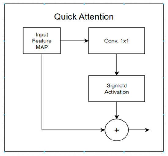
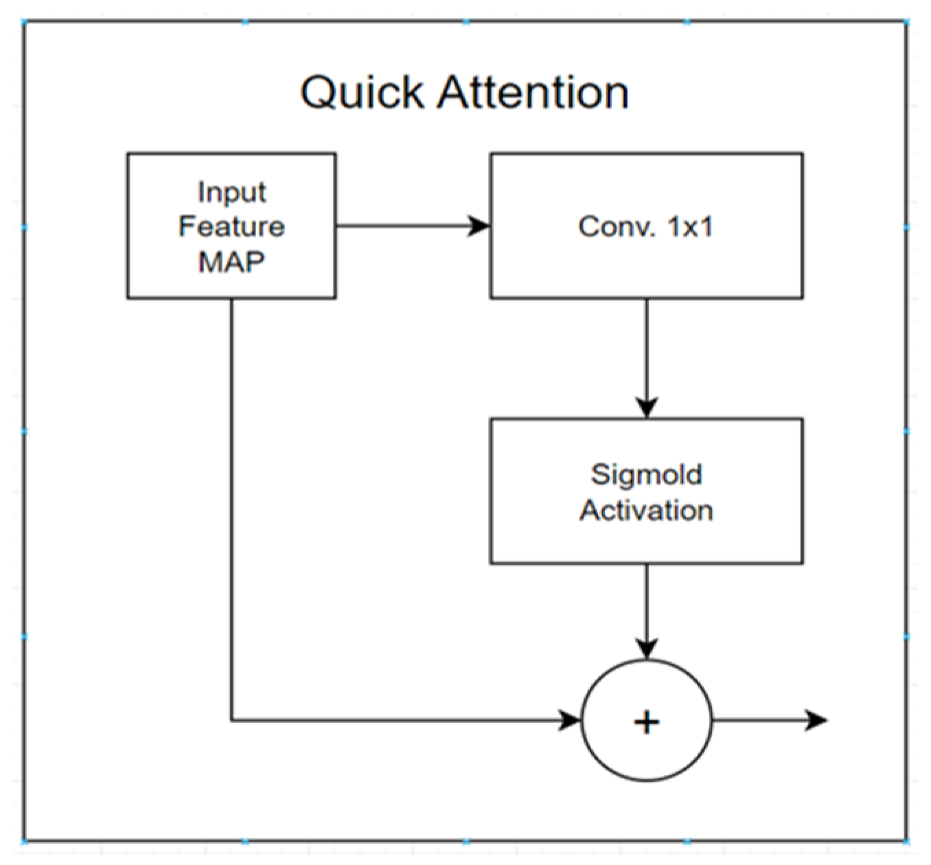
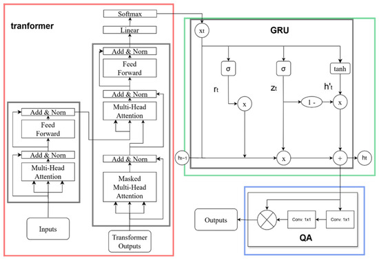
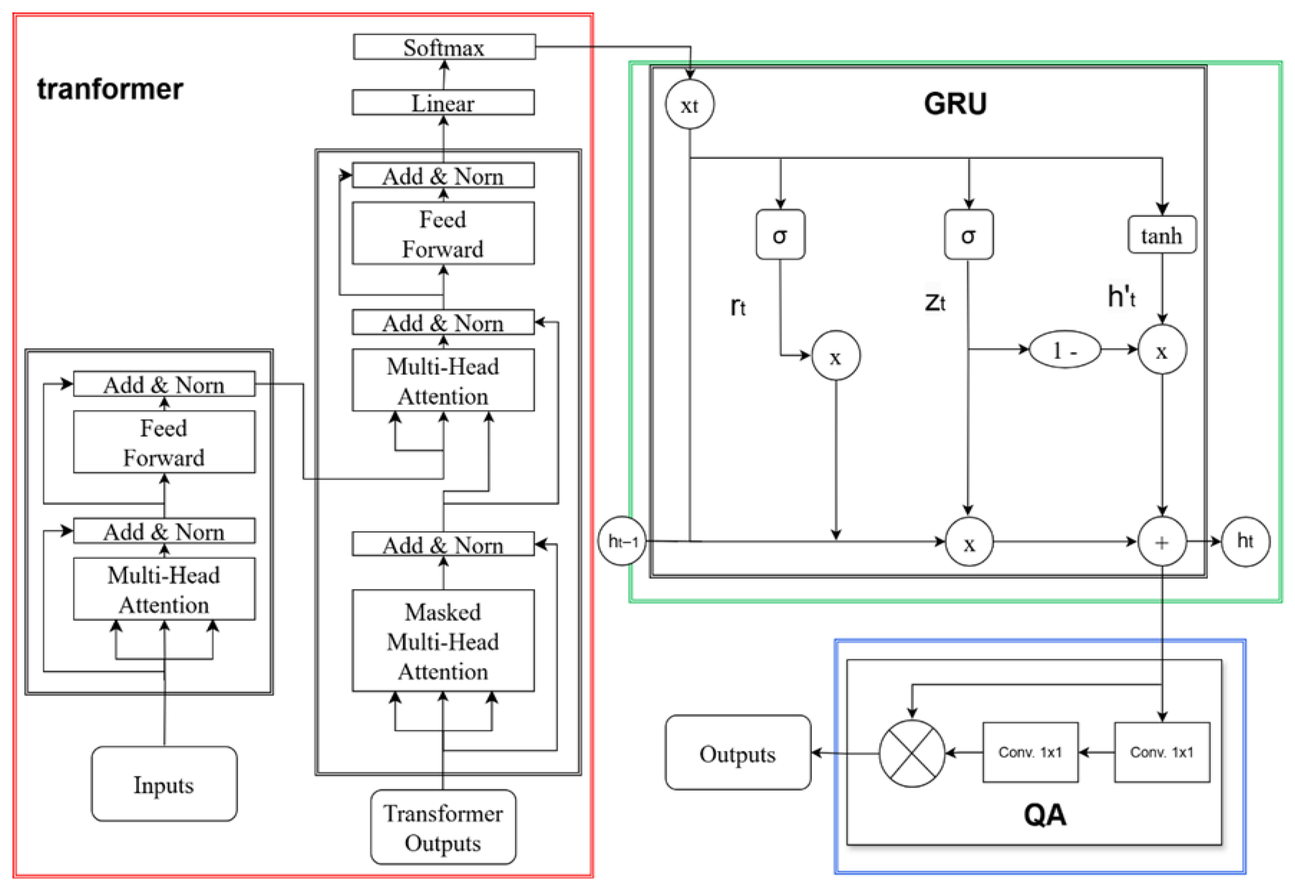
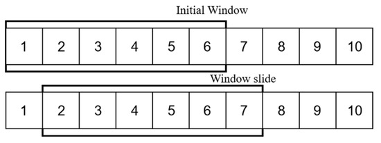
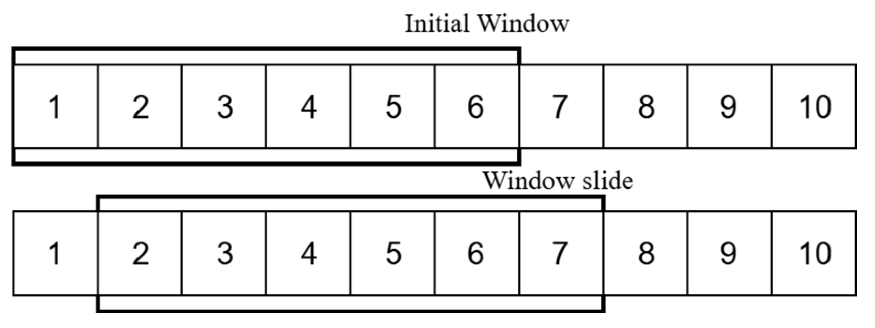
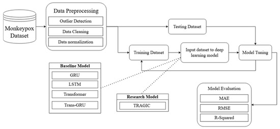
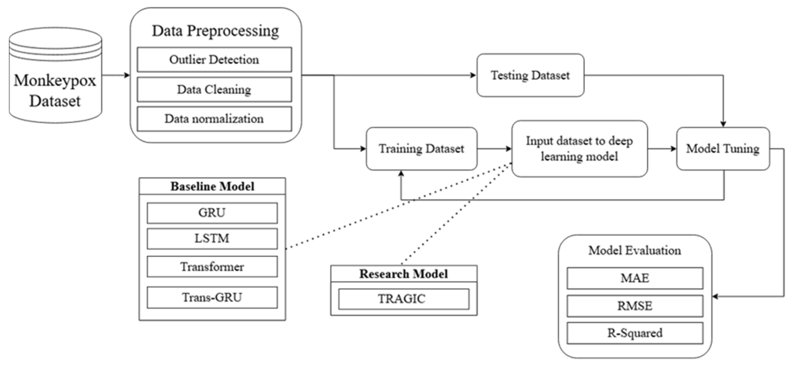
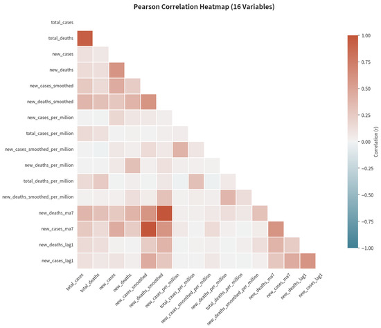
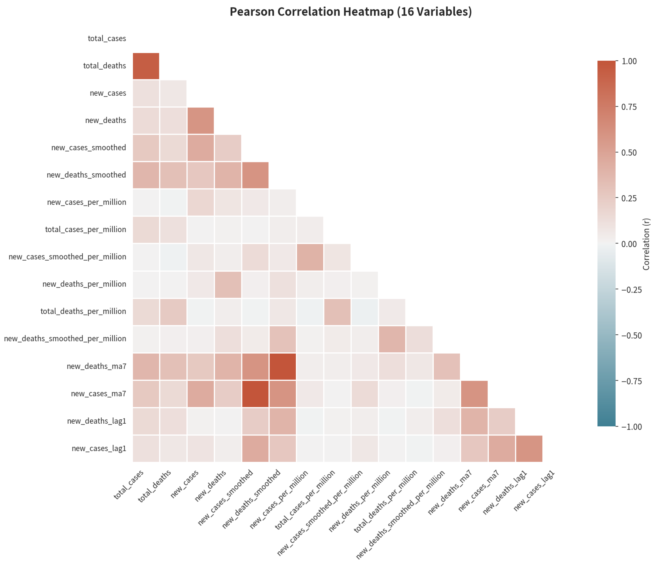
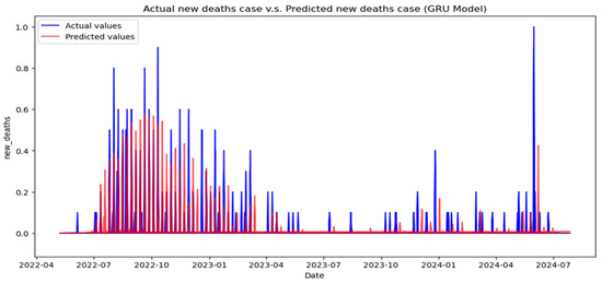
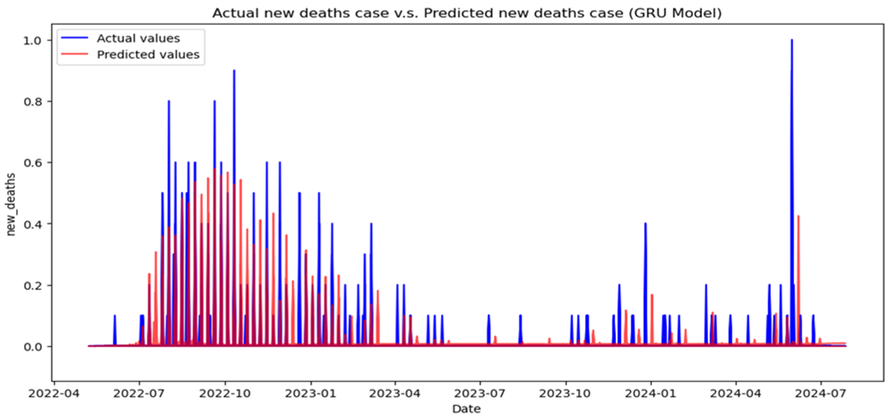
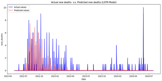
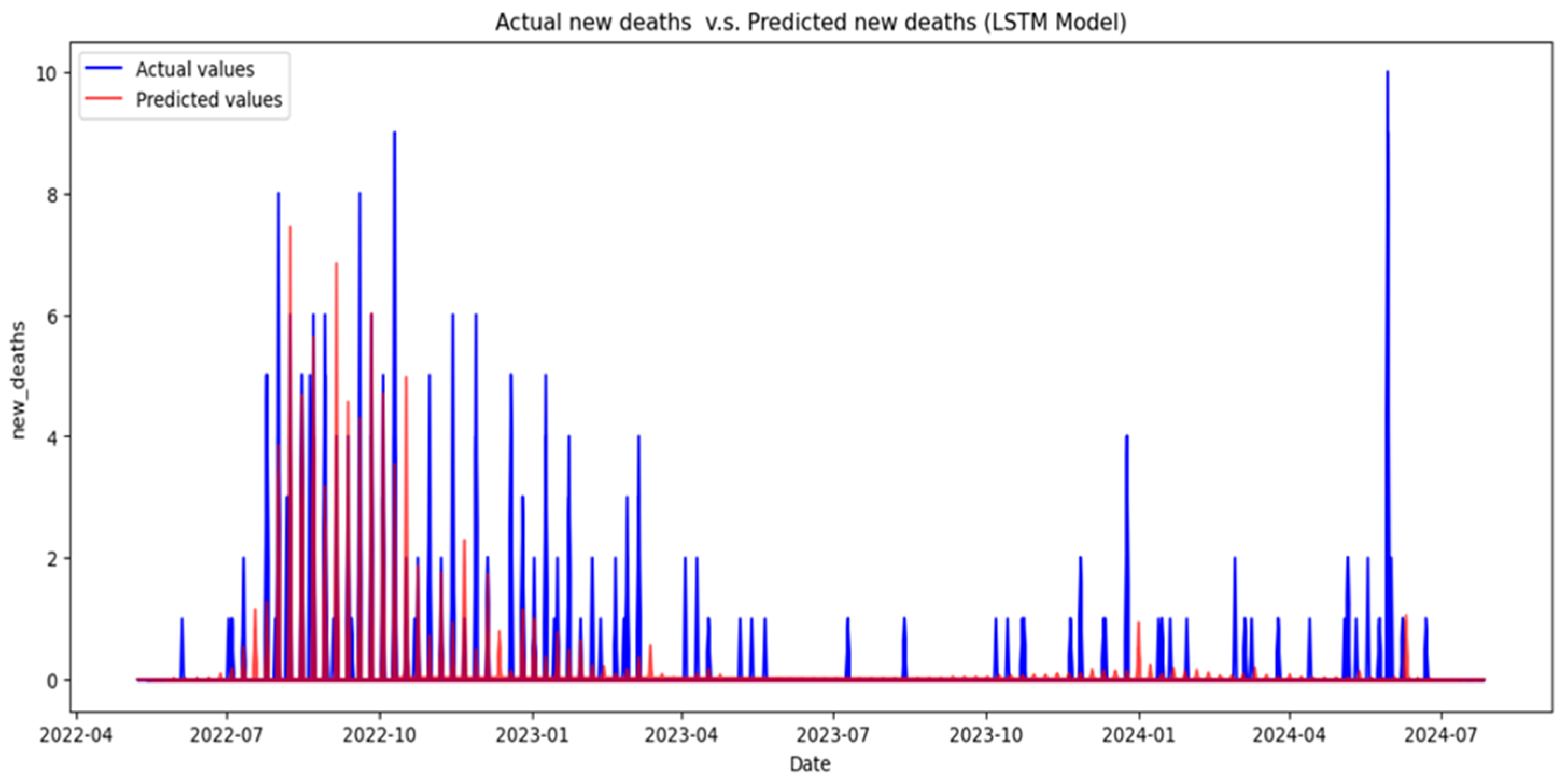
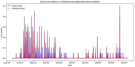
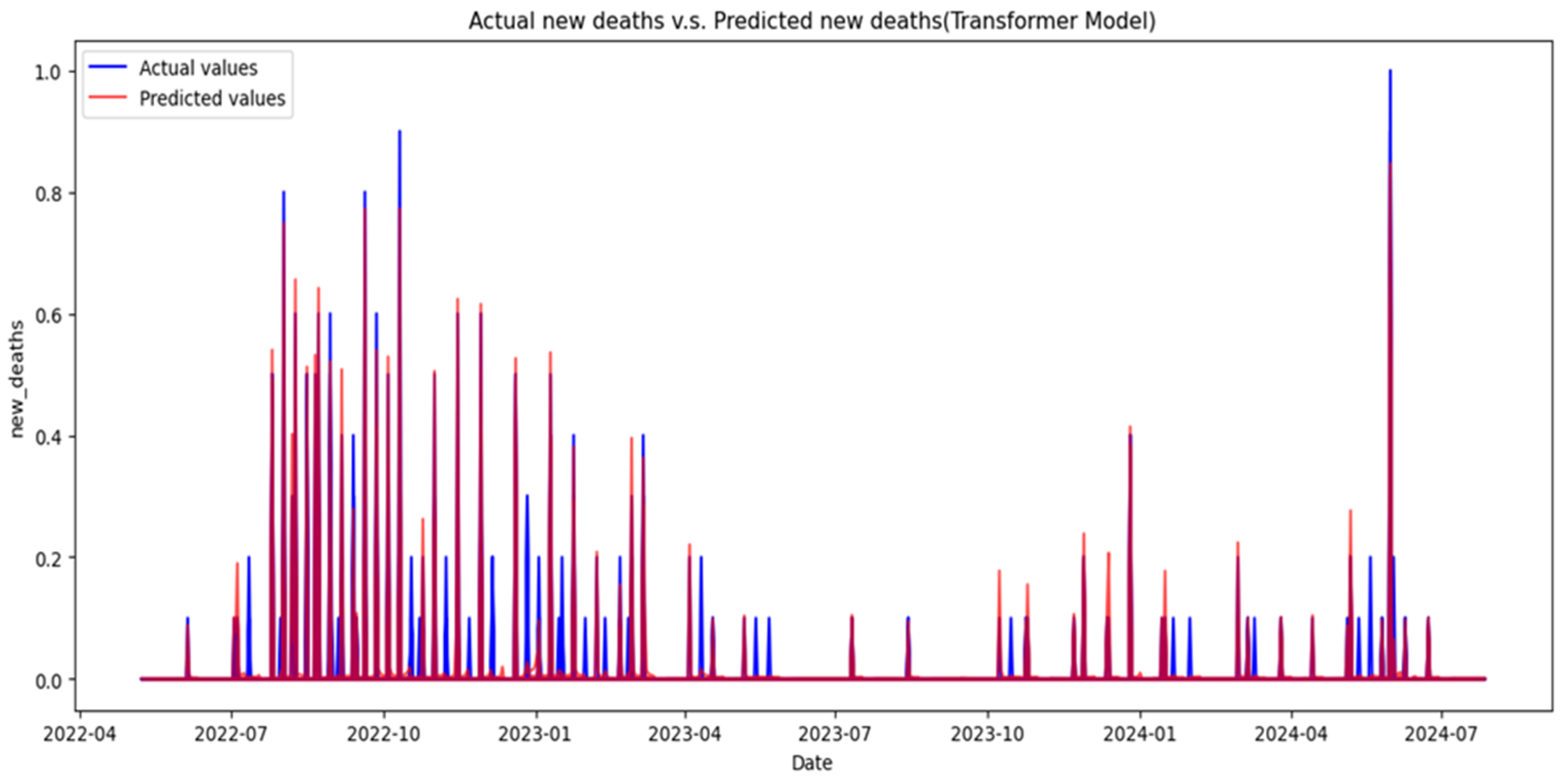
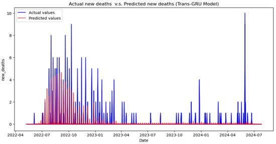
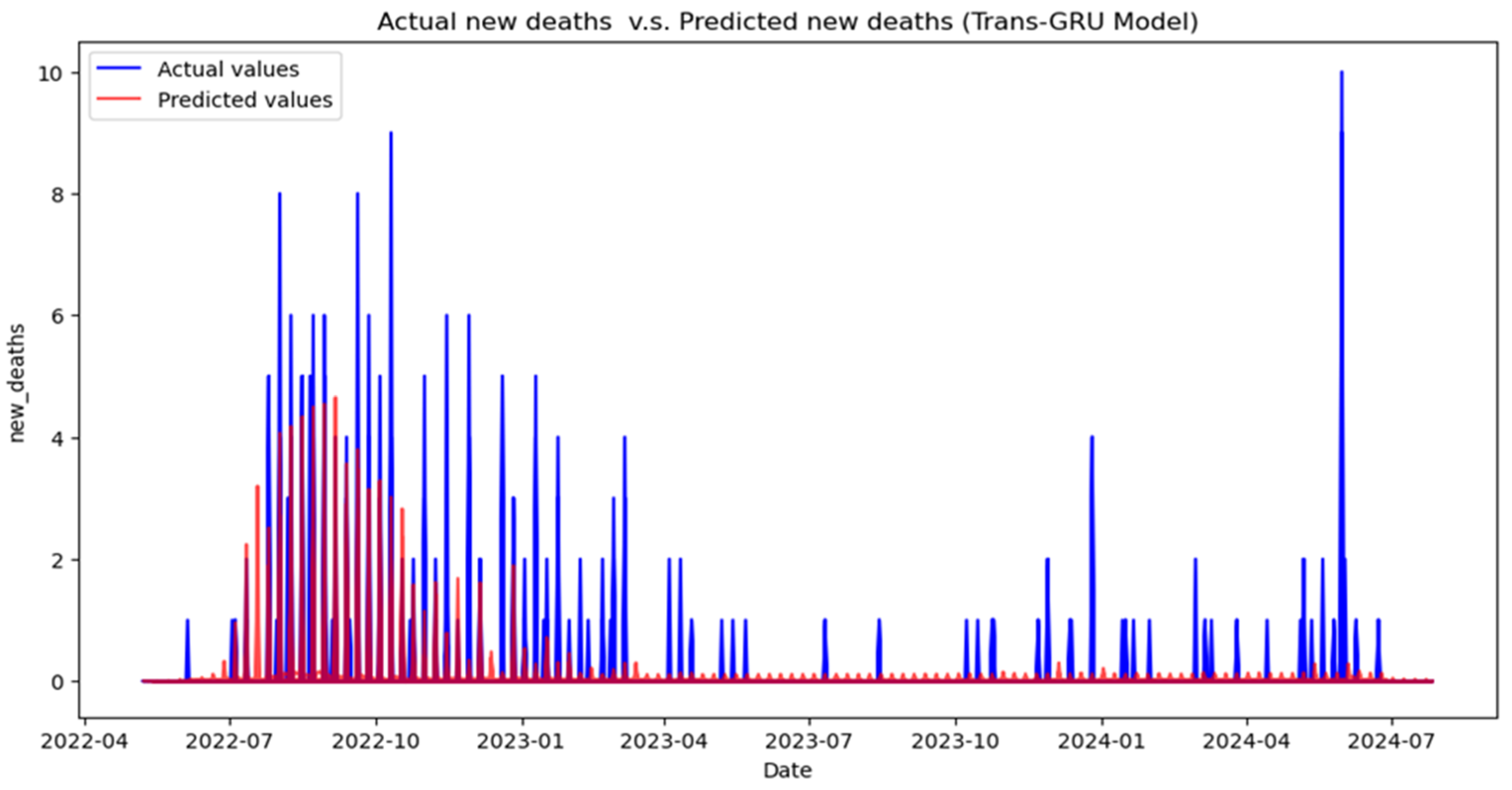
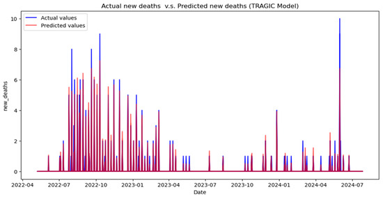
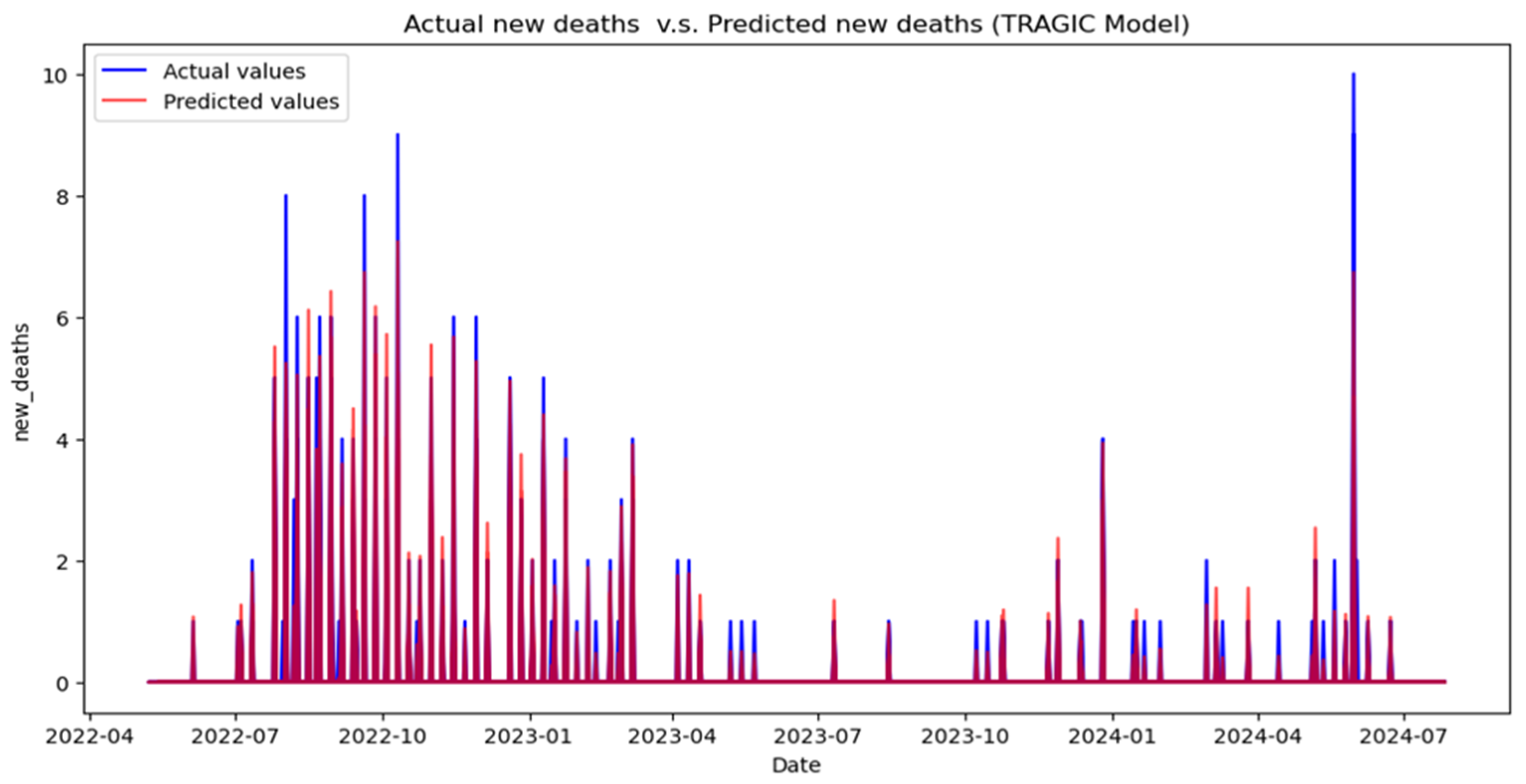
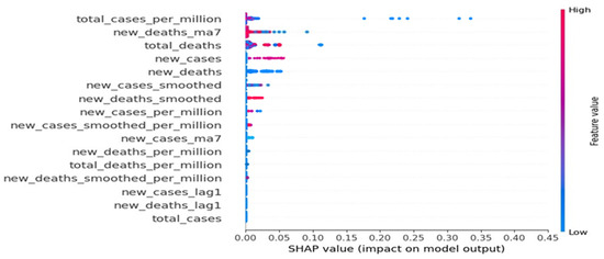
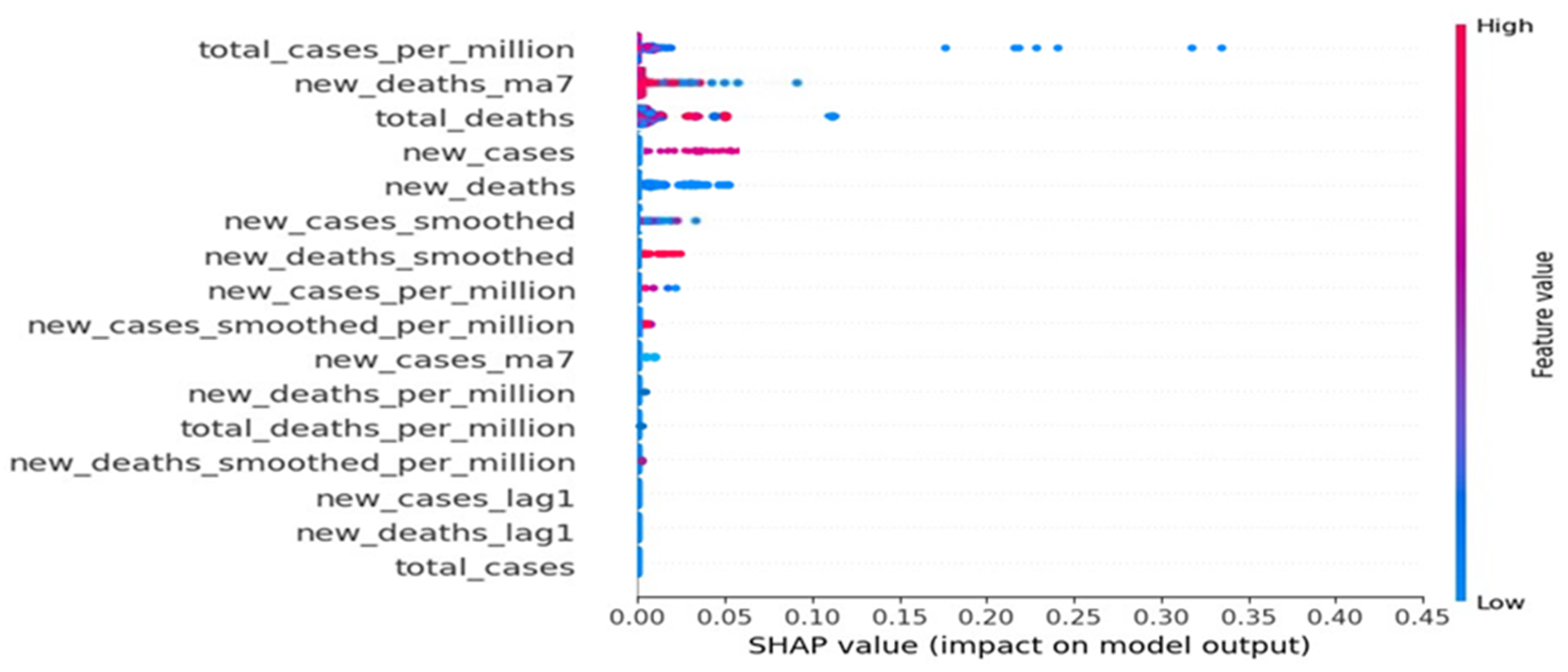

Disclaimer/Publisher’s Note: The statements, opinions and data contained in all publications are solely those of the individual author(s) and contributor(s) and not of MDPI and/or the editor(s). MDPI and/or the editor(s) disclaim responsibility for any injury to people or property resulting from any ideas, methods, instructions or products referred to in the content. |
© 2026 by the authors. Licensee MDPI, Basel, Switzerland. This article is an open access article distributed under the terms and conditions of the Creative Commons Attribution (CC BY) license.