Rational-Power Shifted Lagrangian Distribution for Count Data with Flexible Dispersion

Abstract

The rational-power shifted Lagrangian distribution and its corresponding regression model are discrete Lagrange probability distributions. The proposed model is constructed from a shifted Lagrangian framework with a rational-power component that introduces an additional shape parameter and provides greater flexibility in modeling dispersion and tail behavior. The derivation of the distribution is presented, and its main statistical properties are discussed, together with maximum likelihood estimation based on the expected Fisher information matrix. Using this distribution, a rational-power shifted Lagrangian regression model is formulated for analyzing count data. Simulation results are used to examine the performance of the parameter estimators and to compare the proposed model with the Poisson and modified Sunil models. A real data application using domestic violence data is also provided to illustrate its practical usefulness. The proposed model has a better fit and lower information criteria than the competing models, suggesting it could be used to model overdispersed count data.

1. Introduction

Count data naturally arise in various fields, such as epidemiology, actuarial science, environmental studies, demography, and the social sciences. The Poisson distribution is often used as a model for count responses due to its mathematical properties [1]. However, the assumption of equidispersion, where the mean and variance are expected to be equal, is frequently violated in real-world situations. Empirical count data often show an excess, underabundance, or overabundance of zeros, which makes the Poisson model inadequate. The limitations of the Poisson framework in handling overdispersed data are well documented [2,3,4]. Furthermore, extensive research has been conducted on formal testing procedures aimed at addressing overdispersion and zero inflation [5,6,7,8].

Many generalizations have been proposed to address the Poisson assumption’s dispersion limitations. Alternatives to the Poisson assumption for dispersion include negative binomial, generalized, and asymmetric models [3,9,10]. Furthermore, to address the prevalence of excess zeros frequently seen in various applications, zero-inflated and hurdle models have been developed [7,11]. To further enhance practical applications and improve inference, a wide range of statistical software and regression frameworks are available for modeling count data [12,13].

A systematic approach to developing adaptable discrete models relies on Lagrangian probability distributions. The Lagrangian probability distribution is a class of discrete distributions generated through the Lagrange inversion formula applied to a functional equation of the form $z=ug\left(z\right)$, where $g\left(z\right)$ is a generating function. Various families of these distributions are derived from Lagrange expansions, as explored in [14,15], which provide a thorough examination of their theoretical foundations. Recent advancements have broadened the applications of discrete Lagrange-based models. For instance, [16] examined generating function constructions through two-variable Lagrange expansions, while their applications in statistical modeling are discussed in [17]. Developments in generalized and Lagrangian-type discrete distributions have been widely studied in the literature of statistical modeling [15].

Recent contributions to flexible discrete modeling have concentrated considerable attention on the Weibull distribution and its extensions. By introducing the modified Sunil (MS) distribution, [18] presented a new class of count models capable of accommodating various dispersion patterns. The MS distribution has a probability mass function (PMF) given by

$$P(X=x)={\displaystyle \frac{1}{1+2x}}\left({\displaystyle \genfrac{}{}{0pt}{}{m(1+2x)}{x}}\right)p^{m(1+2x)}{\left({\displaystyle \frac{q}{p}}\right)}^x,x=0,1,2,\dots ,$$

(1)

where $p+q=1$, $0<p<1$, $m=1,2,\dots$. This distribution is derived via a transformation of the original Sunil distribution and serves as a benchmark for comparison with the proposed model. Among the extensions and inferential developments that have emerged are the MS distribution [18], including zero-inflated count data models, and comparative performance analyses [2]. These works highlight the necessity of developing new discrete families within the Lagrangian framework to enhance modeling flexibility.

Despite these advances, there remains a continuing need for count distributions that can simultaneously capture complex dispersion structures, asymmetric patterns, and zero-inflation [18]. Motivated by this study, this paper introduces a novel flexible count distribution known as the rational-power shifted Lagrangian (RPSL) distribution. The proposed model is a specific instance of the shifted Lagrangian (SL) construction that incorporates a rational-power transformation, notably enhancing tail behavior and flexibility in dispersion control. The resulting distribution provides enhanced adaptability for modeling overdispersed count data. Additionally, several modern models are included as particular examples or limiting forms.

The remainder of the paper is organized as follows. Section 2 presents the construction of the SL distribution. Section 3 introduces the RPSL distribution and derives its main statistical properties. Section 4 discusses the moment properties and maximum likelihood estimation. Section 5 develops Fisher-information-based joint inference procedures. Section 6 presents the method of moments estimation. Section 7 reports the results of a simulation study assessing the finite-sample performance of the proposed estimators. Section 8 provides a real data application illustrating the practical usefulness of the model. Concluding remarks and directions for future research are given in Section 9.

2. Shifted Lagrangian Distribution Construction

We propose a new class of Lagrangian probability distributions generated through a shifted probability-generating function of the form

$$g\left(z\right)=c+(1-c)h\left(z\right),0<c<1,$$

(2)

where $h\left(z\right)$ is a successively differentiable function satisfying $h\left(1\right)=1$ and $h\left(0\right)\ne 0$. This construction ensures that $g\left(0\right)=c+(1-c){(1-\theta )}^{\gamma }\ne 0\mathrm{and}g\left(1\right)=1$ accommodate a positive probability mass at zero while preserving the normalization necessary for Lagrangian probability models. Let $z=\psi \left(u\right)$ denote the smallest root of the Lagrangian functional equation $z=ug\left(z\right)$. Then, $\psi \left(u\right)$ defines the probability-generating function (PGF) of a discrete random variable X via the Lagrange inversion formula:

$$\psi \left(u\right)={\displaystyle \sum _{x=1}^{\infty }}{\displaystyle \frac{u^x}{x!}}{\left.D^{x-1}{\left[g\left(z\right)\right]}^x\right|}_{z=0},$$

which provides that

$${\left.D^{x-1}{\left[g\left(z\right)\right]}^x\right|}_{z=0}\ge 0,\mathrm{for}\mathrm{all}x=1,2,\dots .$$

Accordingly, the associated PMF is

$$P(X=x)={\displaystyle \frac{1}{x!}}{\left.D^{x-1}{\left[g\left(z\right)\right]}^x\right|}_{z=0},x=1,2,\dots .$$

(3)

Although (3) defines the PMF for $x=1,2,\dots$, the proposed generator $g\left(z\right)$ with $g\left(0\right)\ne 0$ implies a positive probability at zero, given by $P(X=0)=\psi \left(0\right)=g\left(0\right)$. This is a standard property of Lagrangian distributions when $g\left(0\right)\ne 0$ (see [15]). Thus, the full PMF is $P(X=0)=g\left(0\right)$, and for $x=1,2,\dots$, as in (3).

In the following, we adopt a parametric form of $h\left(z\right)$ to obtain a flexible and analytical Lagrangian distribution with adaptable dispersion and tail behavior.

3. Rational-Power Shifted Lagrangian Distribution

Let

$$g\left(z\right)=c+(1-c)h\left(z\right),0<c<1,$$

(4)

where

$$\begin{array}{c}\hfill h\left(z\right)={\left({\displaystyle \frac{1-\theta }{1-\theta z}}\right)}^{\gamma },0<\theta <1,\gamma >0.\end{array}$$

This generator satisfies

$$g\left(0\right)=c+(1-c){(1-\theta )}^{\gamma }\ne 0\mathrm{and}g\left(1\right)=1.$$

The parameters $\theta$ and $\gamma$ control the shape and tail behavior, providing flexibility for overdispersed or underdispersed data sets. The rational-power generator (RPG) in (2) can be viewed as a special case of the general SL framework (2), where $h\left(z\right)$ determines tail behavior and dispersion.

The full PMF of the RPSL distribution is given by $P(X=0)=g\left(0\right)=c+(1-c){(1-\theta )}^{\gamma }$, and for $x=1,2,\dots$, by Theorem 1.

Theorem 1.

Consider $g\left(z\right)$ as defined in (4). Then, the PMF of the associated distribution is given by

$$\begin{array}{c}\hfill P(X=x)={\displaystyle \frac{c^x}{x}}{\theta }^{x-1}{\displaystyle \sum _{n=0}^x}\left({\displaystyle \genfrac{}{}{0pt}{}{x}{n}}\right){\left[{\displaystyle \frac{1-c}{c}}{(1-\theta )}^{\gamma }\right]}^n\left({\displaystyle \genfrac{}{}{0pt}{}{n\gamma +x-2}{x-1}}\right),x=1,2,\dots .\end{array}$$

(5)

Proof. 

See Appendix A for proof.    □

The PMF is obtained from the PGF $\psi \left(u\right)$ as shown in (5), where $\psi \left(1\right)=1$. It follows that the PMF sums to 1. In particular, ${\sum }_{x=1}^{\infty }P(X=x)=1-g\left(0\right)$ and $P(X=0)=g\left(0\right)$. As a result, ${\sum }_{x=0}^{\infty }P(X=x)=1$. The non-negativity of $P(X=x)$ for $x=1,2,\dots$ is a consequence of the parameter constraints $0<c<1$, $0<\theta <1$, and $\gamma >0$, which confirms that all terms in the sum are non-negative.

3.1. Relationship to Existing Lagrangian Distributions

The RPSL distribution, as defined in Theorem 1, is part of the extensive class of SL distributions as described by [15]. Within this general framework, a random variable X follows an SL distribution if its probability-generating function (PGF) satisfies a functional equation of the form $z=ug\left(z\right)$, where $g\left(z\right)$ is a probability-generating function satisfying $g\left(1\right)=1$. The RPSL construction $g\left(z\right)=c+(1-c){[(1-\theta )/(1-\theta z)]}^{\gamma }$ represents a specific parametric instance of this general class. However, several structural and practical distinctions characterize the RPSL framework relative to the standard SL formulations previously studied in the literature.

Closed-form PMFs of Lagrangian distributions with polynomial, exponential, or simple rational functions $g\left(z\right)$ can be expressed in terms of elementary functions or hypergeometric series [15,17]. In contrast, the RPSL generator incorporates a rational-power transformation of the form ${[(1-\theta )/(1-\theta z)]}^{\gamma }$, where $\gamma >0$ is not necessarily an integer. As noted following Corollary 1, for general $\gamma >0$, the PMF contains terms involving $\Gamma (n\gamma +x-1)$, which generally leads to generalized hypergeometric-type expressions rather than the simpler forms commonly obtained in classical Lagrangian models. This rational-power parameterization results in a wider variety of generalized hypergeometric-type distributions, providing greater flexibility in tail decay rates when compared to polynomial-based or integer-power Lagrangian models.

In many SL constructions, the parameters primarily arise through the generating mechanism and may not separately control zero-mass allocation and tail behavior [14]. By contrast, the RPSL parameters admit clear interpretations: $c\in (0,1)$ directly controls the probability mass at zero via $P(X=0)=c+(1-c){(1-\theta )}^{\gamma }$; $\theta \in (0,1)$ governs the decay rate of the generating function’s poles; and $\gamma >0$ modulates the tail heaviness and dispersion flexibility. This interpretability enhances practical applicability in empirical count data modeling.

Lagrangian distributions have found primary applications in branching processes, queueing theory, genetic models, and ecological population studies [15,17]. The RPSL framework, while mathematically nested within this general class, is specifically tailored to count data exhibiting overdispersion with flexible zero modification, as commonly encountered in epidemiology, actuarial science, and environmental studies (see Section 1). Consequently, the RPSL distribution offers a parsimonious yet flexible alternative when standard Lagrangian models become restrictive in simultaneously capturing tail behavior, dispersion, and zero-mass variability.

Corollary 1.

For $\gamma =1$ in (5), the PMF reduces to the hypergeometric form

$$\begin{array}{c}\hfill P(X=x)=c^x{\theta }^{x-1}A{}_{2}F_1(1-x,x;2;-A),x=1,2,\dots ,\end{array}$$

(6)

where $A=(1-c)(1-\theta )/c$.

Proof. 

See Appendix B for proof.    □

Note that, for general $\gamma >0$, the presence of the term $\Gamma (n\gamma +x-1)$ in the binomial coefficient $\left({\displaystyle \genfrac{}{}{0pt}{}{n\gamma +x-2}{x-1}}\right)$ prevents reduction to the standard Gauss hypergeometric form. Thus, the PMF belongs to a broader class of generalized hypergeometric-type distributions.

3.2. Properties of the Proposed Distribution

In this subsection, we derive some important statistical properties of the proposed distribution, such as moments and dispersion measures. The probability-generating function together with the associated Lagrangian functional equation leads to explicit expressions for the mean, variance, and third central moment.

3.2.1. Mean, Variance, and Third Moment

Let X denote a random variable following the proposed Lagrangian distribution generated in (5). According to Consul and Famoye [15], the mean $\mu =E\left(X\right)$ and variance ${\sigma }^2=\mathrm{Var}\left(X\right)$ of a Lagrangian distribution are given by

$$\begin{array}{cc}\hfill \mu & ={\displaystyle \frac{1}{1-g^{\prime }\left(1\right)}},\hfill \end{array}$$

(7)

$$\begin{array}{cc}\hfill {\sigma }^2& ={\displaystyle \frac{g^{\prime }\left(1\right)}{{(1-g^{\prime }\left(1\right))}^2}}+{\displaystyle \frac{g^{″}\left(1\right)}{{(1-g^{\prime }\left(1\right))}^3}},\hfill \end{array}$$

(8)

where $g^{\prime }\left(z\right)$ and $g^{″}\left(z\right)$ denote the first and second derivatives of $g\left(z\right)$, respectively. By differentiating $g\left(z\right)$ with respect to z, it follows that

$$\begin{array}{c}\hfill g^{\prime }\left(z\right)=(1-c)\gamma \theta {(1-\theta )}^{\gamma }{(1-\theta z)}^{-(\gamma +1)},\end{array}$$

(9)

and evaluating this Equation (9) at $z=1$ results in

$$\begin{array}{c}\hfill g^{\prime }\left(1\right)=(1-c)\gamma \theta {(1-\theta )}^{-1}.\end{array}$$

(10)

The second derivative of $g\left(z\right)$ is

$$\begin{array}{c}\hfill g^{″}\left(z\right)=(1-c)\gamma (\gamma +1){\theta }^2{(1-\theta )}^{\gamma }{(1-\theta z)}^{-(\gamma +2)},\end{array}$$

(11)

and substituting $z=1$ into the Equation (11) gives

$$\begin{array}{c}\hfill g^{″}\left(1\right)=(1-c)\gamma (\gamma +1){\theta }^2{(1-\theta )}^{-2}.\end{array}$$

(12)

By utilizing expressions (7), (8), (10), and (12), the mean and variance of the proposed distribution are obtained as

$$\begin{array}{cc}\hfill \mu & ={\displaystyle \frac{1-\theta }{(1-\theta )-(1-c)\gamma \theta }},\hfill \end{array}$$

(13)

$$\begin{array}{cc}\hfill {\sigma }^2& ={\displaystyle \frac{(1-c)\gamma \theta (1-\theta )\left[(1-\theta )-(1-c)\gamma \theta \right]+(1-c)\gamma (\gamma +1){\theta }^2(1-\theta )}{{\left[(1-\theta )-(1-c)\gamma \theta \right]}^3}}.\hfill \end{array}$$

(14)

The mean $\mu$ is well defined for all $0<c<1$, $0<\theta <1$, $\gamma >0$ provided $(1-\theta )>(1-c)\gamma \theta$, which ensures positivity of the denominator. As $c\to 1^{-}$, $\mu \to 1$, reflecting convergence to a case where all probability mass concentrates at the value 1, but $c=1$ itself is excluded.

For the third raw moment ${\mu }_{\left(3\right)}^{\prime }=E\left(X^3\right)$, the general expression for a Lagrangian distribution is

$$\begin{array}{c}\hfill {\mu }_{\left(3\right)}^{\prime }={\displaystyle \frac{2g^{″}\left(1\right)+6{\left[g^{\prime }\left(1\right)\right]}^2}{{[1-g^{\prime }\left(1\right)]}^3}}+{\displaystyle \frac{g^{″}\left(1\right)+8g^{\prime }\left(1\right)g^{″}\left(1\right)+g^{‴}\left(1\right)}{{[1-g^{\prime }\left(1\right)]}^4}}+{\displaystyle \frac{3{\left[g^{″}\left(1\right)\right]}^2}{{[1-g^{\prime }\left(1\right)]}^5}}.\end{array}$$

(15)

The third derivative of $g\left(z\right)$ is

$$\begin{array}{c}\hfill g^{‴}\left(z\right)=(1-c)\gamma (\gamma +1)(\gamma +2){\theta }^3{(1-\theta )}^{\gamma }{(1-\theta z)}^{-(\gamma +3)},\end{array}$$

(16)

and evaluating this Equation (16) at $z=1$ yields

$$\begin{array}{c}\hfill g^{‴}\left(1\right)=(1-c)\gamma (\gamma +1)(\gamma +2){\theta }^3{(1-\theta )}^{-3}.\end{array}$$

(17)

On substituting $g^{\prime }\left(1\right)$, $g^{″}\left(1\right)$, and $g^{‴}\left(1\right)$ from (10), (12), and (17) into (15) and simplifying, it gives the following closed-form expression:

$$\begin{array}{c}\hfill {\mu }_{\left(3\right)}^{\prime }={\displaystyle \frac{N_3}{{\left[(1-\theta )-(1-c)\gamma \theta \right]}^5}},\end{array}$$

(18)

where

$$\begin{array}{cc}\hfill N_3=& {(1-\theta )}^2\left[2(1-c)\gamma (\gamma +1){\theta }^2+6{(1-c)}^2{\gamma }^2{\theta }^2\right]{\left[(1-\theta )-(1-c)\gamma \theta \right]}^2\hfill \\ \hfill & +(1-\theta )[(1-c)\gamma (\gamma +1){\theta }^2(1-\theta )+8{(1-c)}^2{\gamma }^2(\gamma +1){\theta }^3\hfill \\ \hfill & +(1-c)\gamma (\gamma +1)(\gamma +2){\theta }^3]\left[(1-\theta )-(1-c)\gamma \theta \right]\hfill \\ \hfill & +3{(1-c)}^2{\gamma }^2{(\gamma +1)}^2{\theta }^4(1-\theta ).\hfill \end{array}$$

(19)

Equations (18) and (19) give the third moment in closed rational form. The denominator is the fifth power of $D=(1-\theta )-(1-c)\gamma \theta$. The denominator has the same structure as the mean and variance. The three groups of terms in $N_3$ represent the contributions of ${\left[g^{\prime }\left(1\right)\right]}^3$, $g^{\prime }\left(1\right)g^{″}\left(1\right)$, and $g^{‴}\left(1\right)$ derived from the Lagrange expansion. This explicit form enables direct skewness computation and method of moments estimation. Together with (13) and (14), these expressions confirm that the moments depend explicitly on c, $\theta$, and $\gamma$, offering substantial distributional flexibility.

3.2.2. Overdispersion, Underdispersion, and Equidispersion

The dispersion characteristics of the proposed Lagrangian distribution are examined by comparing its variance ${\sigma }^2$ with its mean $\mu$. The distribution is said to exhibit overdispersion when ${\sigma }^2>\mu$, underdispersion when ${\sigma }^2<\mu$, and equidispersion when ${\sigma }^2=\mu$. From the expression of the mean given in (13), it follows that the mean is finite and positive provided that

$$(1-c)\gamma \theta <1-\theta .$$

(20)

All dispersion comparisons are therefore made under condition (20), which ensures that

$$\begin{array}{c}\hfill D=(1-\theta )-(1-c)\gamma \theta ,\end{array}$$

(21)

which must be positive. By applying the expressions for the mean and variance given in (13) and (14), where

$$\begin{array}{c}\hfill {\sigma }^2={\displaystyle \frac{(1-c)\gamma \theta (1-\theta )D+(1-c)\gamma (\gamma +1){\theta }^2(1-\theta )}{D^3}},\mu ={\displaystyle \frac{1-\theta }{D}}.\end{array}$$

The condition for overdispersion is obtained by comparing ${\sigma }^2$ and $\mu$ as follows:

$$\begin{array}{c}\hfill {\sigma }^2>\mu ⟺{\displaystyle \frac{(1-c)\gamma \theta (1-\theta )D+(1-c)\gamma (\gamma +1){\theta }^2(1-\theta )}{D^3}}>{\displaystyle \frac{1-\theta }{D}}.\end{array}$$

(22)

Under condition (20), multiplying both sides of (22) by $D^3>0$ gives

$$\begin{array}{c}\hfill (1-c)\gamma \theta (1-\theta )D+(1-c)\gamma (\gamma +1){\theta }^2(1-\theta )>(1-\theta )D^2.\end{array}$$

(23)

Dividing both sides of the Equation (23) by $(1-c)\gamma \theta (1-\theta )$, which is greater than zero, yields

$$\begin{array}{c}\hfill D+(\gamma +1)\theta >{\displaystyle \frac{D^2}{(1-c)\gamma \theta }}.\end{array}$$

Since $D=(1-\theta )-(1-c)\gamma \theta$, the left-hand side simplifies to

$$D+(\gamma +1)\theta =(1-\theta )-(1-c)\gamma \theta +(\gamma +1)\theta =1+c\gamma \theta .$$

and therefore the overdispersion condition becomes

$$1+c\gamma \theta >{\displaystyle \frac{D^2}{(1-c)\gamma \theta }}.$$

(24)

Equivalently, multiplying (24) by $(1-c)\gamma \theta$, which is non-negative, the condition reduces to a more compact form of

$$(1-c)\gamma \theta (1+c\gamma \theta )>D^2,$$

(25)

where $D=(1-\theta )-(1-c)\gamma \theta$.

The distribution is equidispersed when equality holds in (25) and underdispersed when the inequality is reversed. Hence, within the admissible parameter space defined by (20), the proposed RPSL distribution is capable of modeling overdispersed, equidispersed, and underdispersed count data, demonstrating substantial flexibility for heterogeneous count processes.

4. Parameter Estimation

Parameter estimation for the proposed Lagrangian distribution can be performed using two standard approaches, namely the method of moments and maximum likelihood estimation (MLE). This section presents both methods for estimating the model parameters $\gamma$, $\theta$, and c.

4.1. Estimating $\gamma$ or $\theta$ When c Is Known

When the parameter c is known, the method of moments can be used to estimate either $\gamma$ or $\theta$, provided the remaining parameter is fixed. Recall that the mean of the proposed RPSL distribution is given by

$$\mu ={\displaystyle \frac{1-\theta }{(1-\theta )-(1-c)\gamma \theta }},(1-c)\gamma \theta <1-\theta .$$

(26)

Let $\overline{y}$ denote the sample mean. Equating the population mean in (26) to the sample mean yields

$$\overline{y}={\displaystyle \frac{1-\theta }{(1-\theta )-(1-c)\gamma \theta }}.$$

(27)

4.1.1. Estimating $\gamma$ When $\theta$ Is Known

Given that c is known and assuming $\theta$ is also known, solving (27) for $\gamma$ gives the moment estimator

$$\tilde{\gamma }={\displaystyle \frac{(1-\theta )(\overline{y}-1)}{(1-c)\theta \overline{y}}}.$$

(28)

Expression (28) provides a simple moment-based estimator for $\gamma$ based on the sample mean $\overline{y}$ and the known values of $\theta$ and c.

4.1.2. Estimating $\theta$ When $\gamma$ Is Known

Since c is assumed known, and now taking $\gamma$ to be known, solving (27) for $\theta$ yields the moment estimator

$$\tilde{\theta }={\displaystyle \frac{\overline{y}-1}{(\overline{y}-1)+\overline{y}(1-c)\gamma }}.$$

(29)

Expression (29) provides a moment-based estimator for $\theta$ based on the sample mean $\overline{y}$ and the known values of $\gamma$ and c.

4.2. Estimating c When $\gamma$ and $\theta$ Are Known

When the parameters $\gamma$ and $\theta$ are known, the method of moments can be used to estimate the shift parameter c. Solving (27) for c yields the moment estimator

$$\tilde{c}=1-{\displaystyle \frac{(\overline{y}-1)(1-\theta )}{\overline{y}\gamma \theta }}.$$

(30)

The estimator $\tilde{c}$ in (30) must satisfy $0<\tilde{c}<1$ to ensure admissibility of the distribution. This condition can be verified directly from the data and the known values of $\gamma$ and $\theta$.

4.3. MLE for $\gamma$, $\theta$, and c

An alternative approach for estimating the parameters $\gamma$, $\theta$, and c is via MLE. Let $Y_1,\dots ,Y_n$ be a random sample from the proposed RPSL distribution with PMF $f(y;\gamma ,\theta ,c)$. The likelihood function is given by

$$\begin{array}{cc}\hfill L(\gamma ,\theta ,c)& ={\displaystyle \prod _{i=1}^n}f(y_i;\gamma ,\theta ,c)\hfill \\ \hfill & ={\displaystyle \prod _{i=1}^n}{\displaystyle \frac{c^{y_i}{\theta }^{y_i-1}}{y_i}}{\displaystyle \sum _{k=1}^{y_i}}\left({\displaystyle \genfrac{}{}{0pt}{}{y_i}{k}}\right){\left[{\displaystyle \frac{1-c}{c}}{(1-\theta )}^{\gamma }\right]}^k\left({\displaystyle \genfrac{}{}{0pt}{}{k\gamma +y_i-2}{y_i-1}}\right).\hfill \end{array}$$

(31)

Define

$$\begin{array}{c}\hfill S(y_i;\gamma ,\theta ,c)={\displaystyle \sum _{k=1}^{y_i}}\left({\displaystyle \genfrac{}{}{0pt}{}{y_i}{k}}\right){\left[{\displaystyle \frac{1-c}{c}}{(1-\theta )}^{\gamma }\right]}^k\left({\displaystyle \genfrac{}{}{0pt}{}{k\gamma +y_i-2}{y_i-1}}\right).\end{array}$$

Then, the likelihood function in (31) can be written compactly as

$$L(\gamma ,\theta ,c)={\displaystyle \prod _{i=1}^n}{\displaystyle \frac{c^{y_i}{\theta }^{y_i-1}}{y_i}}S(y_i;\gamma ,\theta ,c).$$

Latent-Variable Likelihood Representation and Score Functions

Let $Y_1,\dots ,Y_n$ be independent observations from the proposed model. The log-likelihood function is given by

$$\ell (\gamma ,\theta ,c)={\displaystyle \sum _{i=1}^n}logf\left(y_i\right),$$

where $f\left(y_i\right)$ is the PMF defined in Appendix C. The MLEs $\widehat{\gamma }$, $\widehat{\theta }$, and $\widehat{c}$ are obtained by solving the system of score equations

$${\displaystyle \frac{\partial \ell (\gamma ,\theta ,c)}{\partial \gamma }}=0,{\displaystyle \frac{\partial \ell (\gamma ,\theta ,c)}{\partial \theta }}=0,{\displaystyle \frac{\partial \ell (\gamma ,\theta ,c)}{\partial c}}=0.$$

(32)

These equations in (32) do not admit closed-form solutions. Consequently, the MLEs of $\gamma$, $\theta$, and c must be obtained numerically using iterative optimization techniques such as the Newton–Raphson method or other gradient-based algorithms. Note that the detailed derivations of the latent-variable representation, the score functions for $\gamma$, $\theta$, and c, and the resulting system of score equations are provided in Appendix C.

4.4. Expected Fisher Information Matrix

Let $\mathsf{\eta }={(\gamma ,\theta ,c)}^{\top }$ denote the parameter vector. For this three-parameter model, the expected Fisher information matrix is a $3\times 3$ symmetric matrix defined as

$$\mathcal{I}\left(\mathsf{\eta }\right)=-\mathbb{E}\left[{\displaystyle \frac{{\partial }^2{\ell }_{\mathrm{com}}\left(\mathsf{\eta }\right)}{\partial \mathsf{\eta }\partial {\mathsf{\eta }}^{\top }}}\right],$$

(33)

where the expectation is taken with respect to the conditional distribution of the latent variable $K_i\mid Y_i=y_i$, and ${\ell }_{\mathrm{com}}\left(\mathsf{\eta }\right)$ is the complete-data log-likelihood (see Appendix D for derivations). The diagonal elements of $\mathcal{I}\left(\mathsf{\eta }\right)$ are given by

$$\begin{array}{cc}\hfill {\mathcal{I}}_{\gamma \gamma }& ={\displaystyle \sum _{i=1}^n}\mathbb{E}\left[K_i^2\left\{{\psi }^{\prime }\left(K_i\gamma \right)-{\psi }^{\prime }(K_i\gamma +y_i-1)\right\}\mid Y_i=y_i\right],\hfill \end{array}$$

(34)

$$\begin{array}{cc}\hfill {\mathcal{I}}_{\theta \theta }& ={\displaystyle \sum _{i=1}^n}\left[{\displaystyle \frac{y_i-1}{{\theta }^2}}+{\displaystyle \frac{\gamma }{{(1-\theta )}^2}}\mathbb{E}(K_i\mid Y_i=y_i)\right],\hfill \end{array}$$

(35)

$$\begin{array}{cc}\hfill {\mathcal{I}}_{cc}& ={\displaystyle \sum _{i=1}^n}\left[{\displaystyle \frac{y_i}{c^2}}+\mathbb{E}(K_i\mid Y_i=y_i)\left({\displaystyle \frac{1}{{(1-c)}^2}}-{\displaystyle \frac{1}{c^2}}\right)\right],\hfill \end{array}$$

(36)

where ${\psi }^{\prime }\left(x\right)$ is the trigamma function. The nonzero off-diagonal elements are expressed as follows:

$$\begin{array}{c}\hfill {\mathcal{I}}_{\gamma \theta }={\displaystyle \sum _{i=1}^n}{\displaystyle \frac{1}{1-\theta }}\mathbb{E}(K_i\mid Y_i=y_i),{\mathcal{I}}_{\gamma c}=0,{\mathcal{I}}_{\theta c}=0.\end{array}$$

(37)

Thus, from (34) to (37), the expected Fisher information matrix takes the form

$$\mathcal{I}\left(\mathsf{\eta }\right)=\left(\begin{array}{ccc}{\mathcal{I}}_{\gamma \gamma }& {\mathcal{I}}_{\gamma \theta }& 0\\ {\mathcal{I}}_{\gamma \theta }& {\mathcal{I}}_{\theta \theta }& 0\\ 0& 0& {\mathcal{I}}_{cc}\end{array}\right).$$

The detailed derivations of all second-order derivatives and expectation calculations are provided in Appendix D.

5. Fisher-Information-Based Joint Inference

Let $\mathsf{\eta }={(\gamma ,\theta ,c)}^{\top }$ denote the vector of model parameters and let $\widehat{\mathsf{\eta }}$ be its maximum likelihood estimator. Under standard regularity conditions, $\widehat{\mathsf{\eta }}$ is asymptotically normal with the covariance matrix given by the inverse of the expected Fisher information matrix.

5.1. Asymptotic Inference

The expected Fisher information matrix plays a fundamental role in statistical inference. Under the usual regularity conditions, the MLE $\widehat{\mathsf{\eta }}={(\widehat{\gamma },\widehat{\theta },\widehat{c})}^{\top }$ is consistent and asymptotically normal. Specifically, as $n\to \infty$,

$$\sqrt{n}(\widehat{\mathsf{\eta }}-\mathsf{\eta })\stackrel{d}{\to }{\mathcal{N}}_3\left(\mathbf{0},\mathcal{I}{\left(\mathsf{\eta }\right)}^{-1}\right),$$

where $\mathcal{I}\left(\mathsf{\eta }\right)$ denotes the expected Fisher information matrix. Under standard regularity conditions, such as identifiability, continuity, and differentiability of the log-likelihood, and finite Fisher information, the MLE $\widehat{\mathsf{\eta }}$ is consistent and asymptotically normal with the covariance matrix given by the inverse of the expected Fisher information matrix $\mathcal{I}{\left(\mathsf{\eta }\right)}^{-1}$ (see [19,20]). This asymptotic property justifies the use of Wald tests and confidence intervals in the simulation study. Consequently, the asymptotic covariance matrix of $\widehat{\mathsf{\eta }}$ is

$$\mathrm{Var}\left(\widehat{\mathsf{\eta }}\right)\approx \mathcal{I}{\left(\mathsf{\eta }\right)}^{-1},$$

and the asymptotic standard error of ${\widehat{\eta }}_j$ is given by

$$\mathrm{SE}\left({\widehat{\eta }}_j\right)=\sqrt{{\left[\mathcal{I}{\left(\mathsf{\eta }\right)}^{-1}\right]}_{jj}}.$$

5.2. Wald Tests

Let $H_0:\mathit{R}\mathsf{\eta }=\mathit{r}$ be a general null hypothesis, where $\mathit{R}$ is a $q\times 3$ matrix of full row rank and $\mathit{r}$ is a known vector.

The Wald test statistic is defined as

$$W={(\mathit{R}\widehat{\mathsf{\eta }}-\mathit{r})}^{\top }{\left[\mathit{R}\mathcal{I}{\left(\widehat{\mathsf{\eta }}\right)}^{-1}{\mathit{R}}^{\top }\right]}^{-1}(\mathit{R}\widehat{\mathsf{\eta }}-\mathit{r}),$$

which converges in distribution to a ${\chi }_q^2$ random variable under $H_0$. That is, under $H_0$, it satisfies

$$W\stackrel{d}{\to }{\chi }_q^2.$$

In particular, when testing a single parameter, such as under $H_0:\gamma ={\gamma }_0$, the Wald statistic reduces to

$$W_{\gamma }={\displaystyle \frac{{(\widehat{\gamma }-{\gamma }_0)}^2}{\mathrm{Var}\left(\widehat{\gamma }\right)}},$$

where $\mathrm{Var}\left(\widehat{\gamma }\right)$ is the $(1,1)$ entry of $\mathcal{I}{\left(\widehat{\mathsf{\eta }}\right)}^{-1}$.

5.3. Joint Confidence Regions

A $(1-\alpha )$ joint confidence region for the parameter vector $\mathsf{\eta }$ is given by

$$\left\{\mathsf{\eta }:{(\widehat{\mathsf{\eta }}-\mathsf{\eta })}^{\top }\mathcal{I}\left(\widehat{\mathsf{\eta }}\right)(\widehat{\mathsf{\eta }}-\mathsf{\eta })\le {\chi }_{3,1-\alpha }^2\right\},$$

where ${\chi }_{3,1-\alpha }^2$ denotes the $(1-\alpha )$ quantile of the chi-square distribution with three degrees of freedom.

This region has an elliptical shape centered at $\widehat{\mathsf{\eta }}$ and accounts for the joint variability and dependence among $\gamma$, $\theta$, and c.

5.4. Parameter Correlation Assessment

The asymptotic correlation between parameter estimates ${\widehat{\eta }}_i$ and ${\widehat{\eta }}_j$ is obtained from the inverse Fisher information matrix as

$$\mathrm{Corr}({\widehat{\eta }}_i,{\widehat{\eta }}_j)={\displaystyle \frac{{\left[\mathcal{I}{\left(\widehat{\mathsf{\eta }}\right)}^{-1}\right]}_{ij}}{\sqrt{{\left[\mathcal{I}{\left(\widehat{\mathsf{\eta }}\right)}^{-1}\right]}_{ii}{\left[\mathcal{I}{\left(\widehat{\mathsf{\eta }}\right)}^{-1}\right]}_{jj}}}},i\ne j.$$

Large absolute values of these correlations indicate strong dependence between parameter estimators.

6. Method of Moments

When $\gamma$, $\theta$, and c are all unknown, they can be estimated simultaneously using the method of moments by equating the first three sample moments to the corresponding population moments.

6.1. Equating the Sample Mean to the Population Mean

Let $\overline{y}$ denote the sample mean. Equating $\overline{y}$ to the population mean gives

$$\overline{y}={\displaystyle \frac{1-\theta }{(1-\theta )-(1-c)\gamma \theta }}.$$

(38)

6.2. Equating the Sample Variance to the Population Variance

Consider D in (21). The population variance of the proposed RPSL distribution is

$${\sigma }^2={\displaystyle \frac{(1-c)\gamma \theta (1-\theta )D+(1-c)\gamma (\gamma +1){\theta }^2(1-\theta )}{D^3}}.$$

(39)

Let $s^2$ denote the sample variance. Equating $s^2$ to ${\sigma }^2$ yields

$$s^2={\displaystyle \frac{(1-c)\gamma \theta (1-\theta )D+(1-c)\gamma (\gamma +1){\theta }^2(1-\theta )}{D^3}}.$$

(40)

6.3. Equating the Third Sample Raw Moment

Let

$$m_3={\displaystyle \frac{1}{n}}{\displaystyle \sum _{i=1}^n}{y}_i^3$$

denote the third sample raw moment. The corresponding population third moment is given by

$${\mu }_3^{\prime }={\displaystyle \frac{N_3}{D^5}},$$

(41)

where $N_3$ is as stated in (19). On equating $m_3$ to ${\mu }_3^{\prime }$, it follows that

$$m_3={\mu }_3^{\prime }.$$

(42)

The resulting system of nonlinear Equations (38)–(42) can be solved numerically to obtain the method of moments estimators $\tilde{\gamma }$, $\tilde{\theta }$, and $\tilde{c}$. However, several conditions must be satisfied for a valid solution to exist. In particular, the sample moments must lie within the admissible theoretical range defined by $\overline{y}>1$ and $s^2>0$, and $m_3$ must be compatible with the mean and variance. Existence of a solution is not guaranteed if these conditions are violated. Moreover, uniqueness cannot be established analytically, although numerical evidence suggests that the system is well behaved over most of the parameter space. Potential failure cases include: (i) $\overline{y}\le 1$, for which no solution exists; (ii) $s^2=0$, corresponding to boundary cases such as $c\to 1$ or $\theta \to 0$; and (iii) lack of convergence of numerical algorithms near the parameter boundaries. In such situations, MLE is recommended.

6.4. Regression Structure for the RPSL Model

Let ${\mathbf{x}}_i={(1,x_{i1},\dots ,x_{ip})}^{\top }$ denote the vector of covariates for the i-th observation. We model the conditional mean using the log-link function

$$\mu \left({\mathbf{x}}_i\right)=E(Y_i\mid {\mathbf{x}}_i)=exp\left({\mathsf{\beta }}^{\top }{\mathbf{x}}_i\right),$$

where $\mathsf{\beta }={({\beta }_0,{\beta }_1,\dots ,{\beta }_k)}^{\top }$ is the vector of regression coefficients. The mean of the RPSL distribution is given by

$$E\left(Y_i\right)={\displaystyle \frac{1-\theta }{(1-\theta )-(1-c)\gamma \theta }}.$$

To incorporate covariates into the model, we equate the conditional mean to the distributional mean:

$$\mu \left({\mathbf{x}}_i\right)={\displaystyle \frac{1-\theta }{(1-\theta )-(1-c)\gamma \theta }}.$$

By solving for $(1-c)\gamma \theta$, it yields

$$(1-c)\gamma \theta =(1-\theta )\left(1-{\displaystyle \frac{1}{\mu \left({\mathbf{x}}_i\right)}}\right).$$

Hence, the parameter c can be expressed as a function of the covariates:

$$c\left({\mathbf{x}}_i\right)=1-{\displaystyle \frac{1-\theta }{\gamma \theta }}\left(1-{\displaystyle \frac{1}{\mu \left({\mathbf{x}}_i\right)}}\right).$$

(43)

Since c must satisfy $0<c<1$ for a valid RPSL distribution, the regression specification requires that the parameter space be restricted such that, for all i,

$$0<1-{\displaystyle \frac{1-\theta }{\gamma \theta }}\left(1-{\displaystyle \frac{1}{\mu \left({\mathbf{x}}_i\right)}}\right)<1.$$

Equivalently,

$$0<{\displaystyle \frac{1-\theta }{\gamma \theta }}\left(1-{\displaystyle \frac{1}{\mu \left({\mathbf{x}}_i\right)}}\right)<1.$$

Under the parameter restrictions adopted in this paper and the covariate ranges considered in both the simulation study and applications, this condition is satisfied, ensuring that $c\left({\mathbf{x}}_i\right)\in (0,1)$, and the model is well defined.

This formulation induces a covariate-dependent parameter $c\left({\mathbf{x}}_i\right)$ through the mean structure, while the shape parameters $\gamma$ and $\theta$ remain constant across observations. By substituting (43) into the PMF, the RPSL regression model is given by

$$\begin{array}{cc}\hfill P(Y_i=y_i\mid {\mathbf{x}}_i)& ={\displaystyle \frac{c{\left({\mathbf{x}}_i\right)}^{y_i}}{y_i}}{\displaystyle \sum _{n=0}^{y_i}}\left({\displaystyle \genfrac{}{}{0pt}{}{y_i}{n}}\right){\left[{\displaystyle \frac{1-c\left({\mathbf{x}}_i\right)}{c\left({\mathbf{x}}_i\right)}}{(1-\theta )}^{\gamma }\right]}^n\hfill \\ \hfill & \times \left({\displaystyle \genfrac{}{}{0pt}{}{n\gamma +y_i-2}{y_i-1}}\right){\theta }^{y_i-1},y_i=1,2,\dots .\hfill \end{array}$$

The likelihood function for a random sample $\mathbf{y}=(y_1,\dots ,y_n)$ is

$$L\left(\mathsf{\beta }\right)={\displaystyle \prod _{i=1}^n}P(Y_i=y_i\mid {\mathbf{x}}_i).$$

The corresponding log-likelihood function is

$$\ell (\mathsf{\beta })={\displaystyle \sum _{i=1}^n}\left[y_{i}logc\left({\mathbf{x}}_i\right)-log{y}_i+log\left({\displaystyle \sum _{n=0}^{y_i}}\left({\displaystyle \genfrac{}{}{0pt}{}{y_i}{n}}\right){\left[{\displaystyle \frac{1-c\left({\mathbf{x}}_i\right)}{c\left({\mathbf{x}}_i\right)}}{(1-\theta )}^{\gamma }\right]}^n\left({\displaystyle \genfrac{}{}{0pt}{}{n\gamma +y_i-2}{y_i-1}}\right){\theta }^{y_i-1}\right)\right].$$

The score functions for the regression coefficients $\mathsf{\beta }$ are derived in Appendix E using the chain rule and the conditional expectation $\mathbb{E}(K_i\mid Y_i=y_i)$.

7. Simulation Study

A simulation study was conducted to assess the finite-sample performance of the Poisson, MS, and RPSL models. The MS distribution is defined in (1). For the RPSL model, inference was carried out using the maximum likelihood framework based on the latent-variable representation introduced in Section 3.2. In particular, the variance-covariance matrix of the estimators was obtained from the inverse of the expected Fisher information matrix $\mathcal{I}{\left(\mathsf{\eta }\right)}^{-1}$, where $\mathsf{\eta }={(\gamma ,\theta ,c)}^{\top },$ and $\mathcal{I}\left(\mathsf{\eta }\right)$ is defined in (33).

7.1. Simulation Algorithm

An algorithm for generating random samples from the RPSL distribution is given in Algorithm 1. This algorithm is used to evaluate the finite-sample performance of the proposed model and to compare it with competing count distributions. All computations and graphical displays were implemented in the R programming language.

Algorithm 1 Efficient sampling from the RPSL distribution

Require: Parameters $\gamma$, $\theta$, c; sample size N; maximum count $y_{max}$ 1: Precompute the pmf for $y=1,\dots ,y_{max}$: $$P(Y=y)={\displaystyle \frac{c^y}{y}}{\displaystyle \sum _{n=0}^y}\left({\displaystyle \genfrac{}{}{0pt}{}{y}{n}}\right){\left[{\displaystyle \frac{1-c}{c}}{(1-\theta )}^{\gamma }\right]}^n\left({\displaystyle \genfrac{}{}{0pt}{}{n\gamma +y-2}{y-1}}\right){\theta }^{y-1}.$$ 2: Normalize the probabilities: $$p_y={\displaystyle \frac{P(Y=y)}{{\sum }_{k=1}^{y_{max}}P(Y=k)}}.$$ 3: Construct the cumulative distribution function: $$F\left(y\right)={\displaystyle \sum _{k=1}^y}{p}_k.$$ 4: for  $i=1,\dots ,N$  do 5:      Generate $u_i\sim U(0,1)$ 6:      Select $y_i$ such that $$F(y_i-1)<u_i\le F\left(y_i\right).$$ 7: end for 8: Output:  $\{y_1,\dots ,y_N\}\sim \mathrm{RPSL}(\gamma ,\theta ,c)$

7.2. Simulation Study Design

The simulation study is conducted according to the following steps:

• Specify the model parameters $(\gamma ,\theta ,c)$.
• Fix a sufficiently large truncation value for the support of the distribution, for example $y_{max}=500$.
• Compute the PMF and normalize it to obtain a valid discrete distribution.
• Generate random samples using the inverse CDF method described in Algorithm 1.
• Repeat the procedure for different parameter settings in order to examine the effects on skewness, dispersion, and tail behaviour.
• Fit the proposed model and competing count regression models to each generated data set and compute the maximized log-likelihood, AIC, and BIC for comparison.

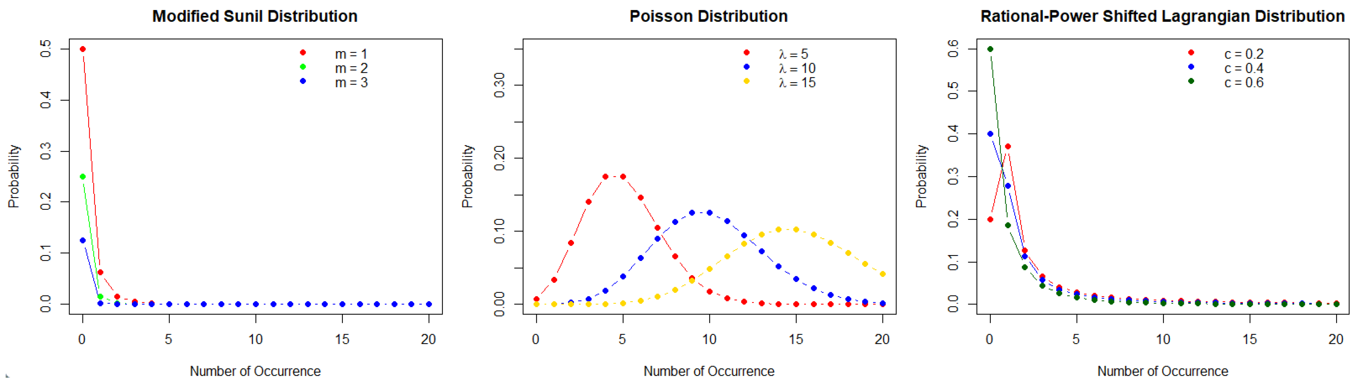
To examine the effect of the model parameters on the distributional shapes, Figure 1 presents the PMFs under different parameter settings. For each sample size $n\in$ 50, 100, 300, 500, a total of $R=500$ replications were generated from the RPSL distribution with true parameter vector ${\mathsf{\eta }}_0={(1.5,0.4,0.3)}^{\top }.$ The parameters $\gamma =1.5$, $\theta =0.4$, and $c=0.3$ are chosen because they satisfy $D=0.18>0$, yield a mean $\mu \approx 3.33$ and zero proportion $\approx 0.625$, and represent a typical overdispersed count data scenario. Small variations around these values do not materially affect the conclusions, as confirmed by additional simulations. For each dataset, the MLE $\widehat{\mathsf{\eta }}={(\widehat{\gamma },\widehat{\theta },\widehat{c})}^{\top }$ was obtained by numerically solving the system of score equations. For each replication and for each component of $\mathsf{\eta }$, the following measures were computed. The bias of an estimator quantifies the average deviation from the true parameter value ${\eta }_{0j}$:

$$\mathrm{Bias}\left({\widehat{\eta }}_j\right)={\displaystyle \frac{1}{R}}{\displaystyle \sum _{r=1}^R}{\widehat{\eta }}_{jr}-{\eta }_{0j}.$$

The mean squared error (MSE) measures the average squared deviation from the true parameter value, combining both variance and bias:

$$\mathrm{MSE}\left({\widehat{\eta }}_j\right)={\displaystyle \frac{1}{R}}{\displaystyle \sum _{r=1}^R}{\left({\widehat{\eta }}_{jr}-{\eta }_{0j}\right)}^2.$$

The coverage probability (CP) is defined as the proportion of replications for which the asymptotic $95\%$ confidence interval contains the true parameter value. Confidence intervals were constructed using the estimated Fisher information matrix:

$$\widehat{\mathsf{\eta }}\pm 1.96\times \mathrm{diag}{\left\{\mathcal{I}{\left(\widehat{\mathsf{\eta }}\right)}^{-1}\right\}}_j^{1/2},$$

where $\mathcal{I}\left(\widehat{\mathsf{\eta }}\right)$ denotes the observed Fisher information matrix evaluated at the maximum likelihood estimate. For model comparison, the Akaike information criterion (AIC) and Bayesian information criterion (BIC) were computed for each fitted model:

$$\begin{array}{c}\hfill \mathrm{AIC}=-2\ell \left(\widehat{\mathsf{\eta }}\right)+2k\mathrm{and}\mathrm{BIC}=-2\ell \left(\widehat{\mathsf{\eta }}\right)+klog\left(n\right),\end{array}$$

where $\ell \left(\widehat{\mathsf{\eta }}\right)$ is the maximized log-likelihood value, k denotes the number of model parameters, and n is the sample size. The best model for each sample size is determined by the smallest AIC and BIC values. The results are reported in

Table 1. Simulation results for Poisson, MS, and RPSL models with 95% coverage probabilities (CP). Best values for MSE, AIC, and BIC are bolded.

n	Model	Est (SD)	Bias	MSE	CP	AIC	BIC
50	Poisson	$\lambda$ = 3.0173 (0.2424)	1.5173	3.3348	0.090	430.0136	431.9257
50	MS	m = 0.6102 (0.1717) p = 0.1830 (0.0485)	−0.8898 −0.2170	0.8643 0.0569	0.085 0.140	217.0005	220.8245
50	RPSL	$\gamma$ = 3.5963 (3.2277) $\theta$ = 0.3439 (0.2082) c = 0.3032 (0.0640)	2.0963 −0.0561 0.0032	16.6154 0.0440 0.0044	0.695 0.760 0.930	207.5873	213.3234
100	Poisson	$\lambda$ = 3.0318 (0.1727)	1.5318	2.9477	0.015	873.3373	875.9425
100	MS	m = 0.5639 (0.1044) p = 0.1664 (0.0318)	−0.9361 −0.2336	0.9030 0.0592	0.015 0.050	434.9066	440.1170
100	RPSL	$\gamma$ = 2.8443 (2.5198) $\theta$ = 0.3455 (0.1724) c = 0.2971 (0.0453)	1.3443 −0.0545 −0.0029	8.8262 0.0271 0.0021	0.845 0.880 0.925	412.7670	420.5825
300	Poisson	$\lambda$ = 3.0881 (0.1012)	1.5881	2.7419	0.000	2726.0775	2729.7813
300	MS	m = 0.5081 (0.0515) p = 0.1446 (0.0165)	−0.9919 −0.2554	0.9894 0.0664	0.000 0.000	1311.2335	1318.6411
300	RPSL	$\gamma$ = 1.9646 (1.0946) $\theta$ = 0.3787 (0.1060) c = 0.3002 (0.0264)	0.4646 −0.0213 0.0002	1.9976 0.0127 0.0008	0.905 0.935 0.950	1237.6160	1248.7273
500	Poisson	$\lambda$ = 3.0215 (0.0776)	1.5215	2.4157	0.000	4417.1431	4421.3577
500	MS	m = 0.5127 (0.0402) p = 0.1467 (0.0129)	−0.9873 −0.2533	0.9777 0.0648	0.000 0.000	2175.7245	2184.1537
500	RPSL	$\gamma$ = 1.7783 (0.7335) $\theta$ = 0.3821 (0.0827) c = 0.2983 (0.0204)	0.2783 −0.0179 −0.0017	0.7249 0.0084 0.0004	0.905 0.935 0.960	2051.4454	2064.0892

Note: Bold values indicate the smallest AIC and BIC results.

.

The RPSL model fits better than the Poisson and MS models, with the lowest AIC and BIC values across all sample sizes. Regarding the RPSL parameters, the estimators for $\theta$ and c demonstrate minimal bias, low MSE, and coverage probabilities that are close to the nominal level, even with moderate sample sizes. The estimator of the shape parameter $\gamma$ shows large variability for small samples ($n=50$ and $n=100$), which results in inflated bias and MSE. As the sample size increases, the expected Fisher information matrix becomes more informative, and the estimator stabilizes. For $n=300$ and $n=500$, the bias and MSE of $\gamma$ decrease sharply, and the CP remains close to the nominal level. In contrast, the Poisson and MS models exhibit substantial bias and extremely low coverage probabilities, reflecting model misspecification. Their MSE values do not improve with increasing sample size in the same way as for the RPSL model.

In general, the simulation results confirm that the proposed likelihood-based inference using the expected Fisher information matrix provides consistent and reliable estimation for the RPSL model and that the proposed distribution offers a markedly better fit than the competing models.

It is noted that the simulation study is focused on the MLE due to its improved statistical efficiency and practical application since it is the main inferential method considered in this work. However, moment-based estimators are developed for theoretical completeness. The method of moment estimators is not efficient in some cases, especially when the sample sizes are small or the data are non-normal. These factors may result in biased estimates and lower reliability of the inference compared to MLE.

7.3. Comparison with Mainstream Overdispersed Models

While the simulation study compares the RPSL distribution with the Poisson and MS models, the negative binomial (NB) and generalized Poisson (GP) are among the most widely used benchmark models for overdispersed count data in the literature [9,21].

However, this study evaluates the proposed RPSL model in the Lagrangian-type family and against the Poisson benchmark, the natural baseline model. Therefore, the simulation design focuses on nested and structurally related models rather than an exhaustive comparison across all competing overdispersed count models.

The superior performance of RPSL over the Poisson model in terms of AIC and BIC, as shown in Table 1, suggests that the rational-power transformation captures overdispersion more effectively than the standard equidispersed framework.

A more comparative study involving models such as NB and GP would require a separate and more extensive simulation design, as these models are based on fundamentally different generative mechanisms. We therefore consider such a comparison an important direction for future research.

Nevertheless, the MS distribution, included in our simulation, represents a recently proposed flexible count model [18] that shares structural similarities with Lagrangian-type constructions and therefore provides a meaningful within-class benchmark. The fact that RPSL outperforms MS across all sample sizes, as documented by Table 1, provides evidence of its advantage within this modeling framework.

8. Application

In this section, we analyze a real dataset using three competing count regression models: Poisson, MS, and RPSL. The objective is to examine the effects of covariates $X_1,\dots ,X_{12}$ on the response variable and to determine which model provides the best fit.

8.1. Data Description

We analyze a domestic violence dataset with 214 observations (Famoye and Singh, 2006).

Table 2. Descriptive statistics.

Variable	Mean	SD
$X_1$ (education, victim)	2.29	0.75
$X_2$ (education, batterer)	2.07	0.78
$X_3$ (employment, victim)	0.50	0.50
$X_4$ (employment, batterer)	0.66	0.48
$X_5$ (income, victim)	2.57	1.31
$X_6$ (income, batterer)	3.07	1.47
$X_7$ (family interaction, victim)	0.82	0.38
$X_8$ (family interaction, batterer)	0.72	0.45
$X_9$ (club membership, victim)	0.27	0.45
$X_{10}$ (club membership, batterer)	0.19	0.39
$X_{11}$ (drug problem, victim)	0.14	0.34
$X_{12}$ (drug problem, batterer)	0.62	0.49
Y (number of incidents)	4.21	10.60

presents descriptive statistics for the response variable Y (number of incidents) and the twelve covariates.

8.2. Regression and Dispersion Estimates

Table 3. Estimated regression coefficients for the Poisson, MS, and RPSL models.

	Poisson		MS		RPSL
Covariate	Estimate	SE	Estimate	SE	Estimate	SE
Intercept	2.7379 ***	0.1689	5.7719	3.2411	0.1052	0.4726
$x_1$	−0.2069 ***	0.0514	−1.1455	0.9407	0.0310	0.1402
$x_2$	−0.3156 ***	0.0471	0.3036	0.5289	0.1339	0.1304
$x_3$	0.3070 ***	0.0821	1.0880	1.2950	−0.0899	0.2277
$x_4$	−0.0417	0.1150	2.0360	1.6914	−0.1298	0.3220
$x_5$	−0.1582 ***	0.0347	−0.6512	0.3471	0.0790	0.0956
$x_6$	−0.0970 *	0.0385	−0.7422	0.5385	0.0565	0.1147
$x_7$	−0.0918	0.0955	−0.5036	1.1798	0.2430	0.2585
$x_8$	−0.6521 ***	0.0701	−1.2322	1.3482	0.1763	0.1961
$x_9$	0.8460 ***	0.0870	2.5842 **	1.1733	−0.4027	0.2683
$x_{10}$	−0.8490 ***	0.1133	−2.1287	1.1791	0.3688	0.3038
$x_{11}$	−0.5235 ***	0.1238	−0.9966	1.1399	0.1575	0.3169
$x_{12}$	1.0049 ***	0.0890	1.3519	0.9183	−0.3899	0.2245

Significance levels: *** $p<0.01$, ** $p<0.05$, * $p<0.10$.

reports the estimated regression coefficients for the three models. For the Poisson model, the overall Wald test strongly rejects the null hypothesis that all slope coefficients are zero (${\chi }^2=479.6$, df = 12, $p<0.001$), with ten covariates individually significant at the 5% level. The estimated intercept corresponds to ${\widehat{\beta }}_0=2.7379$ (SE = 0.1689), which implies a baseline mean of $\widehat{\lambda }=exp\left(2.7379\right)=15.4542$.

The joint Wald test for the slope parameters in the MS model is not significant (${\chi }^2=11.52$, df = 12, $p=0.485$). However, the dispersion parameter $\widehat{m}=50.000$ (SE = 12.204) is highly significant ($p<0.001$ for $H_0$: $m=1$). This suggests overdispersion and provides strong evidence against the Poisson specification.

In the RPSL model, the additional parameter estimates are $\widehat{\gamma }=5.000$ (SE = 3.237) and $\widehat{\theta }=0.3053$ (SE = 0.144). The test for $H_0$: $\theta =0$ is significant ($p=0.034$), whereas $H_0$: $\gamma =1$ is not ($p=0.217$). The joint test of $H_0$: $\gamma =1,\theta =0$ is strongly rejected (${\chi }^2=607.49$, df = 2, $p<0.001$). The slope parameters are not jointly significant (${\chi }^2=9.69$, df = 12, $p=0.643$, indicating that the covariate effects are not statistically significant in this model).

Table 4. Estimates of dispersion and shape parameters.

Parameter	Estimate	SE
m (MS)	50.0000 ***	12.2042
$\gamma$ (RPSL)	5.0000	3.2366
$\theta$ (RPSL)	0.3053 **	0.1442

*** $p<0.01$, ** $p<0.05$.

presents the estimates of the dispersion and shape parameters for the extended models.

Overdispersion makes the MS and RPSL regression coefficients less statistically significant compared to the Poisson model. In cases where the mean and variance differ, the Poisson model often underestimates variability. This underestimation results in overly small standard errors and inflated estimated effects of covariates. The MS and RPSL models overcome this issue by offering more precise variance estimates, resulting in larger standard errors due to the inclusion of additional parameters. When this additional variability is considered, the perceived significance of the Poisson model decreases. The observed effects may result from model misspecification rather than reflecting true underlying relationships. While the extended models provide more reliable inference, they may lead to a reduction in the number of covariates that are statistically significant.

8.3. Model Comparison

Table 5. Model comparison based on log-likelihood and information criteria.

Model	Log-Likelihood	AIC	BIC
Poisson	$-1376.914$	$2779.829$	$2823.586$
MS	$-390.485$	$808.970$	$856.094$
RPSL	$-379.111$	$788.223$	$838.712$

displays the goodness-of-fit metrics for the various models analyzed. The Poisson model has the worst fit, indicating potential overdispersion, with an AIC value of $2779.8$ and a log-likelihood value of $-1376.914$. Compared to the Poisson model, both extended models show notable improvements. The log-likelihood value of the MS model is $-390.485$, with an AIC value of $808.970$ and a BIC value of $856.094$. In contrast, the RPSL model has the highest log-likelihood value of $-379.111$ and the lowest AIC value of $788.223$.

The Poisson regression is inadequate for these data due to overdispersion. The extended models exhibit a markedly superior fit relative to the standard model. The RPSL model achieves the highest log-likelihood and the lowest AIC, indicating superior goodness-of-fit among all competing models. Moreover, the MS model performs adequately with stable estimation, so both the MS and RPSL models are suitable, though the RPSL model provides the best fit to the data.

9. Concluding Remarks

In this paper, we proposed a new flexible count distribution based on the RPSL construction. The additional shape parameter provides greater control over dispersion, skewness, and tail behavior than classical count models while retaining a tractable likelihood function. The Poisson model is obtained as a limiting case, which allows formal model comparison using likelihood-based criteria.

The MLE procedure was developed using the expected Fisher information matrix, and a simulation study was conducted to evaluate the finite-sample performance of the estimators. The results show that the estimators of the parameters associated with dispersion and zero probability exhibit small bias, low MSE, and coverage probabilities close to the nominal level, even for moderate sample sizes. Although the shape parameter shows high variability for small samples, its performance improves rapidly as the sample size increases, confirming the consistency of the proposed inference procedure. The Poisson and MS models exhibit significant bias and exhibit very poor coverage probabilities when the data are generated from the RPSL distribution, indicating a misalignment in model specification.

The analysis of the domestic violence data provides compelling evidence of overdispersion and highlights the practical significance of the proposed model. RPSL demonstrates the highest log-likelihood and the lowest AIC, signifying that it provides the best fit among the models analyzed.

Overall, the proposed distribution considerably enlarges the class of admissible count data models and provides a competitive alternative for analyzing overdispersed data. Possible directions for future research include the development of zero-inflated and hurdle versions of the model, Bayesian estimation procedures, regression models with improved numerical stability, and applications to other types of count data arising in environmental, medical, and social sciences.