


Abstract
Predicting the degradation and lifespan of embedded computers relies critically on the accurate evaluation of key parameter degradation within computing systems. Accelerated high-temperature tests are frequently employed as an alternative to ambient-temperature degradation tests, primarily due to the excessive duration and cost of ambient-temperature testing. However, the scarcity of effective methodologies for correlating degradation trends across distinct temperature conditions persists as a prominent challenge. This study addresses this gap by leveraging adversarial learning to generate low-temperature degradation sequences from high-temperature datasets. The adversarial learning framework enables feature transfer across diverse operating conditions and facilitates domain adaptation learning. This empowers the model to extract features invariant to degradation trends across multiple temperature conditions. Furthermore, soft dynamic time warping (SDTW) is utilized to precisely align the generated low-temperature sequences with their real-world counterparts. This alignment methodology enables elastic matching of time series data exhibiting nonlinear temporal variations, thereby ensuring accurate comparison and synchronization of degradation sequences. Compared with prior methodologies, our proposed approach delivers superior performance on computer degradation data. It offers a more accurate and reliable solution for the degradation analysis and lifespan prediction of embedded computers, thereby advancing the reliability of computational systems.
MSC:
62M10; 37M10
1. Introduction
As space missions grow increasingly complex and diverse, spacecraft-embedded computers have evolved into indispensable components of contemporary aerospace systems. These computers are widely employed in the critical systems of diverse spacecraft, including satellites, probes, and other aerospace vehicles, where they fulfill pivotal roles in flight control, communication, and data processing. They undertake critical functions such as mission management and command execution. Consequently, the performance and reliability of these embedded computers are paramount to the success of space missions [1,2].
Spacecraft-embedded computers operate under extremely harsh conditions in space. They must endure harsh environmental stressors that induce gradual degradation over time [3]. Key parameters—including processor clock frequency, memory read/write speed, and communication interface transmission rate—may degrade under these conditions. For instance, prolonged exposure to elevated temperatures can impair semiconductor devices, resulting in fluctuations in processor clock frequency and increased error rates. Such exposure also impairs the conversion rates of optocoupler components and the accuracy of analog-to-digital (A/D) and digital-to-analog (D/A) conversions. The degradation of these parameters can not only reduce spacecraft operational efficiency but also trigger system failures, potentially compromising the success of space missions.
Degradation of computers under ambient operating conditions is a slow, gradual process. Typically, significant performance degradation may take several years to manifest in ambient temperature environments. Accelerated high-temperature testing can simulate long-term service life within a short timeframe by elevating environmental temperatures, thereby accelerating material aging and the failure of electronic components. According to the Arrhenius equation, chemical reaction rates increase exponentially with increasing temperature—a phenomenon also applicable to the aging of electronic components. Therefore, accelerated high-temperature testing can yield degradation data equivalent to several years or more of ambient-temperature conditions within only a few weeks or months, thereby significantly reducing the testing cycle.
High-temperature accelerated testing is an effective approach for investigating the degradation of key parameters in spacecraft-embedded computers. Ground-based simulation of elevated temperatures significantly accelerates the degradation of these key parameters. This approach empowers researchers to collect extensive degradation data in a short timeframe, facilitating the identification of degradation patterns. For instance, in an elevated-temperature environment, the processor clock frequency degrades more rapidly due to the hot-carrier effect in transistors. Similarly, optocoupler efficiency degrades rapidly due to increased capacitor leakage currents. Additionally, deviations in analog-to-digital (A/D) converters are caused by elevated temperatures’ effects on electronic circuit performance. Data from elevated-temperature tests are crucial for predicting the temporal evolution of computer performance under ambient conditions.
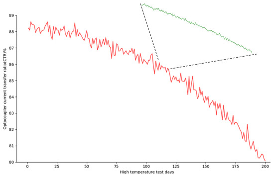
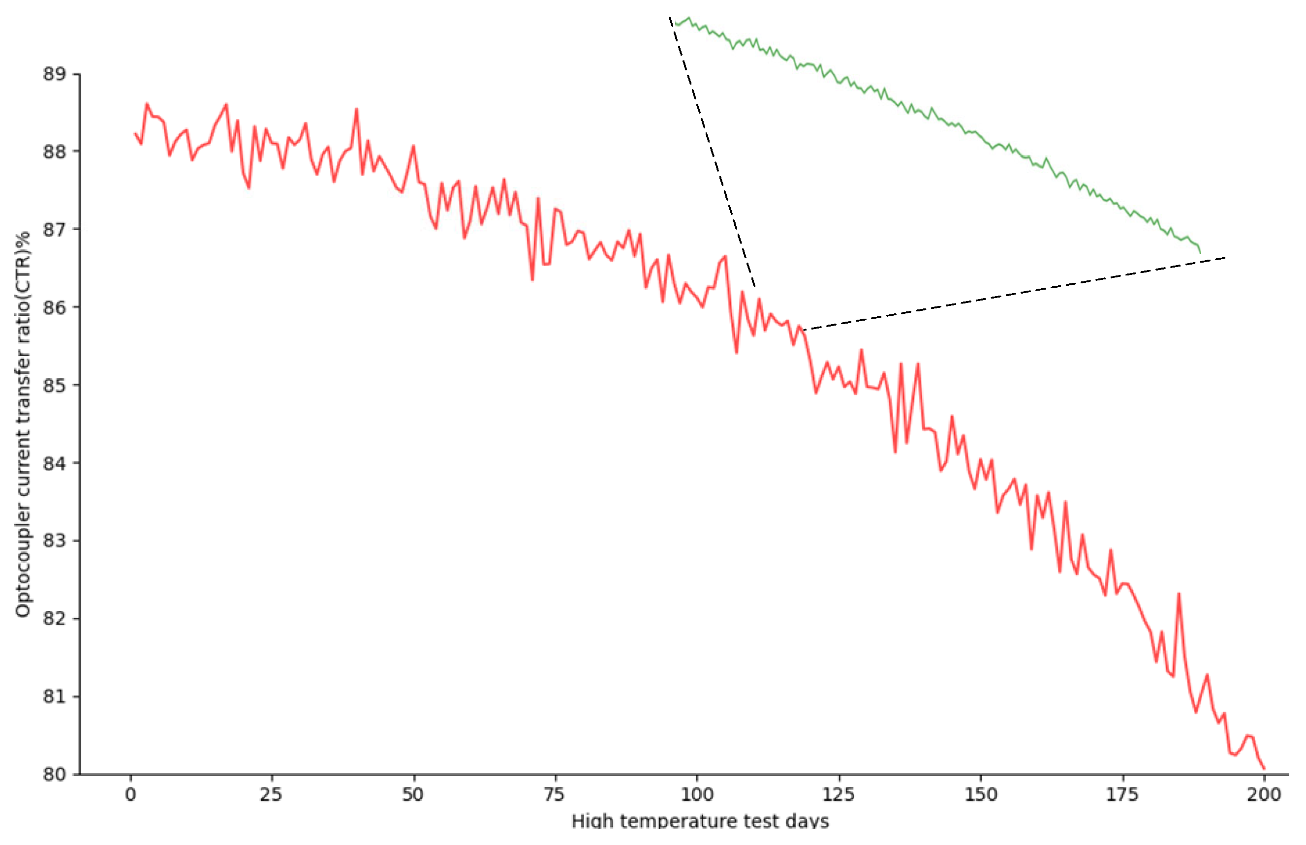
However, no simple linear relationship exists between elevated- and ambient-temperature degradation data, given significant discrepancies in their time scales. For instance, the Current Transfer Ratio (CTR) of on-board optocouplers—defined as output-to-input current ratio—degrades with temperature and time, reflecting natural degradation. Degradation rate at elevated temperatures is substantially faster than under ambient operating conditions. Figure 1 compares degradation curves at 160 °C (short, steep red line) and ambient operating temperatures (extended green line). A core challenge is mapping the elevated-temperature degradation curve to predict the ambient operating curve. For effective data conversion and prediction, establishing a precise, reliable mapping relationship between rapidly varying elevated-temperature degradation time series and slowly evolving ambient-temperature degradation is imperative.
Figure 1.
Optocoupler Current Transfer Ratio (CTR) Degradation Mapping Between Elevated and Ambient Temperatures. A core challenge in degradation research is mapping short-term, severe elevated-temperature degradation (red line) to long-term, slow ambient-temperature degradation (green line). The red curve reflects accelerated CTR degradation under elevated-temperature stress, with rapid declines driven by intensified thermal aging. In contrast, the green curve shows gradual CTR degradation under ambient operating conditions, with a slower decay rate matching real-world service scenarios.
Current traditional methods exhibit limitations in processing these two time-series datasets (which differ in length and variation rates). These limitations include ineffective time-axis alignment and challenges in capturing complex nonlinear mapping patterns. These challenges constrain the mapping and prediction accuracy of degradation data. Thus, exploring novel methods to establish a correlation between elevated- and ambient-temperature degradation data holds significant theoretical and practical value for engineering applications. Such methods improve prediction accuracy of key embedded computer parameter degradation, optimize design and manufacturing processes, reduce research and development (R&D) costs, and ensure successful space mission execution.
Accurately mapping elevated- and ambient-temperature degradation data is a core challenge in research on parameter degradation in spacecraft-embedded computers. The classical Arrhenius equation—an established chemical kinetics model—assumes an exponential temperature-dependent degradation rate. Deep learning, particularly neural network-based models, exhibits significant potential in addressing nonlinear mappings and complex data patterns. Multilayer neural networks can learn complex nonlinear relationships between elevated- and ambient-temperature degradation data. Several studies have utilized convolutional neural networks (CNNs) [4] for local feature extraction and recurrent neural network (RNN)-based models—including long short-term memories (LSTMs) [5], gated recurrent units (GRUs) [6], bidirectional LSTMs (BiLSTMs) [7], and Transformers [8]—to outperform traditional prediction methods. Nevertheless, time-series data on elevated- and ambient-temperature degradation often exhibit distinct patterns and lengths. Current deep learning models struggle to effectively align and compare feature spaces across elevated- and ambient-temperature data. This hinders accurate prediction of ambient-temperature degradation using elevated-temperature data.
Critical gaps remain in current research on embedded computer degradation prediction. First, existing deep learning methods lack mechanisms for extracting domain-invariant features, leading to poor generalization during transfer from elevated- to ambient-temperature data. Second, traditional alignment methods fail to address nonlinear temporal distortions between cross-temperature sequences. No prior work has integrated adversarial learning (for domain adaptation) and soft dynamic time warping (Soft-DTW, for elastic sequence alignment) to solve the cross-temperature degradation mapping problem in embedded computers. This integration is imperative for bridging the gap between accelerated-elevation-temperature data and ambient-temperature operational data.
This study introduces a Generative Adversarial Network (GAN) integrated with soft Dynamic Time Warping (Soft-DTW) to address these limitations and enable accurate degradation mapping and prediction. Our key contributions are summarized as follows:
- We introduce a method for generating ambient-temperature degradation time series via adversarial learning. By constructing an adversarial network that incorporates a feature extractor, a degradation sequence predictor, and a domain discriminator, adversarial learning empowers the feature extractor to learn domain-invariant representations. Specifically, we utilize a Bidirectional Long Short-Term Memory (BiLSTM) network to extract elevated-temperature sequence features, and input the mapped feature vectors into a Gated Recurrent Unit (GRU)-based sequence generator to guide ambient-temperature sequence generation. The generated and real sequences are subsequently fed into the sequence discriminator for adversarial training.
- Under multi-condition settings, embedded computer degradation sequences may exhibit varying degradation rates and nonlinear temporal distortions. Soft-DTW can effectively align sequences with distinct lengths and temporal distortions, accurately capturing similarity between degradation sequences. We incorporate a Soft-DTW loss function during adversarial training to minimize the distance between generated and real sequences, thereby enhancing prediction accuracy and enabling cross-temperature sequence transfer prediction (from elevated to ambient conditions).
This study aims to map key parameter degradation time-series data under both elevated and ambient temperatures for spacecraft-embedded computers. By addressing limitations of existing methods in correlating elevated- and ambient-temperature degradation data and effectively utilizing elevated-temperature accelerated test data, we develop a more accurate prediction model. This model offers a more reliable approach to spacecraft service-life prediction, particularly for key parameters of embedded computers.
The cross-condition degradation time-series generation method achieves high-precision degradation trend generation across distinct conditions by integrating an encoder–decoder architecture into the GAN framework. The BiLSTM encoder and GRU decoder structure can extract operational features and generate realistic degradation trends. Furthermore, integration of Soft-DTW loss enables the model to maintain high adaptability and accuracy when processing variable-length time series and multi-condition data. Compared to conventional methods, this approach significantly reduces prediction errors under multi-condition scenarios and exhibits excellent generation performance in complex cases.
2. Related Works
At operational temperatures, the degradation of aerospace-embedded computers progresses slowly, making significant short-term changes difficult to detect. In contrast, the degradation of critical parameters in these systems accelerates markedly at elevated temperatures due to thermal carrier effects, electromigration, and oxidation reactions. Establishing a quantitative relationship between high-temperature and normal-temperature degradation remains a critical challenge.
2.1. The Arrhenius Equation and Its Modifications in Electronic System Degradation
The Arrhenius equation is used to extrapolate normal-temperature degradation rates from high-temperature degradation rate constants and activation energy. Despite its solid theoretical foundation and parsimonious parameter set, the Arrhenius equation is often inadequate for modeling the complex degradation of spacecraft-embedded computer parameters. Specifically, it assumes a single degradation mechanism with a constant activation energy, an assumption that fails to capture the co-occurrence of multiple mechanisms. Furthermore, it cannot directly process time-series data or fully leverage dynamic degradation information.
Initially used to describe the relationship between temperature and chemical reaction rates, the traditional Arrhenius equation is mathematically expressed as , where represents the temperature-dependent characteristics of chemical reaction rates, A is an estimated constant, is the experimental activation energy, R is the molar gas constant, and T is the thermodynamic temperature. In accelerated life testing, the Arrhenius model is widely used to predict the lifespan of materials and devices. Osterman [9] discusses the application of the Arrhenius equation to the reliability analysis of electronic devices and notes its limitations in high-temperature accelerated aging tests. Wilcoxon [10] discusses the application of the Arrhenius equation in electronic devices and analyzes the impact of temperature on device lifespan. Zhang [11] proposes an Arrhenius equation-based model for predicting the performance of lithium-ion batteries, combining temperature and aging data to predict the remaining life of the battery. Lele [12] uses the Arrhenius equation to predict the aging process of lithium-ion batteries and verifies the accuracy of the model through experiments. Li [13] proposes an SPICE model for phase change memory (PCM) based on the Arrhenius equation and demonstrates its application in circuit design. Kuehl [14] systematically analyzes the aging behavior of thin-film resistors and operational amplifiers at high temperatures. To more accurately describe the degradation patterns of critical parameters in electronic components, researchers have modified the traditional Arrhenius equation. One significant modification involves introducing temperature-dependent activation energy () and a pre-exponential factor (). The modified model is expressed as:
This modification accounts for nonlinear relationships between degradation rates and temperature, addressing cases where constant activation energy assumptions fail. Another critical advancement involves multiphysics field coupling models [15,16]. Since thermal, mechanical, and electrical interactions collectively influence degradation in aerospace-embedded computers, coupled models have been developed:
where represents mechanical stress, V denotes electric field strength, and is a coupling function [17]. Similarly, electro-hydraulic simulations of aero-engine variable stator vane (VSV) actuators confirm servo-valve degradation increases by under combined thermal and mechanical stress [18]. These models enable a more realistic reflection of degradation patterns by incorporating multiphysics interactions.
2.2. Time Series Methods in Electronic System Degradation
A time series is a sequence of data points recorded in chronological order [19]. In degradation research for aerospace-embedded computers, time series typically capture the variation of key parameters, such as processor clock frequency, over time. Each series consists of timestamps and corresponding parameter values, reflecting the dynamic evolution of these parameters.
2.2.1. Traditional Statistical Methods
Traditional statistical methods form the foundation of time-series analysis. The moving average method mitigates short-term fluctuations to reveal underlying trends by computing local averages. Exponential smoothing enhances sensitivity to recent trends by assigning greater weight to recent observations. The Autoregressive Moving Average (ARMA) model and its extension, the Autoregressive Integrated Moving Average (ARIMA) model, model current values as linear functions of past values and random errors, enabling future value prediction through parameter estimation.
The utility of these methods is demonstrated in various applications. Wang [20] employed ARIMA to predict capacitor aging, demonstrating high accuracy and reliability validated across different temperatures. Gorlov [21] utilized ARIMA models to predict transistor degradation from electrostatic discharge or life-test data. Amini [22] applied ARIMA for the simultaneous forecasting of conventional electrical load and electric vehicle charging demand. Hybrid and novel approaches further leverage time-series concepts. Meng [23] presented a framework combining Gaussian process regression (GPR) and a Kalman filter (KF) for battery end-of-life prediction with uncertainty assessment. Ni [24] predicted the remaining useful life of MOSFETs using time-series modeling, incorporating correlation analysis, Akaike Information Criterion (AIC)-based parameter optimization, and short-term cycle prediction. Yin [25] introduced Monotonic Segmented Linear Regression (MSLR), a method designed to capture monotonic degradation trends amidst significant measurement noise, enabling statistically valid upper-bound estimation with high confidence. These methodologies are widely used due to their well-established theoretical foundations and strong interpretability, making them well-suited for time-series data exhibiting linear trends and periodic components.
2.2.2. Deep Learning Methods
Recent advances in deep learning have significantly enhanced time-series analysis. LSTM, a specialized recurrent neural network (RNN) architecture [26], effectively models long-term dependencies through gated mechanisms (input, forget, and output). These gates regulate information flow within memory cells, thereby mitigating the vanishing gradient problem inherent in traditional RNNs. The GRU, a more parameter-efficient alternative to LSTM, similarly excels at capturing long-range temporal dependencies. One-dimensional convolutional neural networks (1D-CNNs) [27] employ sliding kernels to extract local temporal features, offering computational efficiency for large-scale time-series data.
The Transformer architecture, initially developed for natural language processing, uses self-attention mechanisms to capture dependencies between positions in a sequence, regardless of temporal distance. This capability is highly effective for modeling complex, long-term dependencies in time-series data. The model’s inherent parallelizability further enhances its computational efficiency for lengthy sequences. The self-attention mechanism learns the importance and correlations among all time points, generating highly expressive representations. Consequently, numerous Transformer variants, such as the Temporal Fusion Transformer, have been developed for time-series analysis, demonstrating state-of-the-art performance in forecasting and classification.
These architectures have facilitated significant methodological advancements. For instance, Chen [28] proposed MMRNet, which integrates MOSUM, flash-MUSE attention, and RNN cores for multi-horizon prediction of battery capacity degradation. Singh [29] developed a deep learning framework for estimating battery performance parameters, validated across diverse battery technologies and cycling conditions. Gao [30] incorporated total ionizing dose (TID)-induced degradation mechanisms into a Transformer architecture using a customized physics-informed loss function. Mao [31] introduced a concise, channel-independent multivariate forecasting framework, and Mao [32] presented a dual-branch Siamese network enhanced by curriculum learning and transfer learning for long-term prediction of computer parameter degradation. The latter approach minimizes distributional discrepancies through a correlation alignment loss.
Recent advances in Generative Adversarial Network (GAN)-based time series modeling have yielded significant methodological contributions [33]. Yoon et al. [34] proposed TimeGAN, which integrates the unsupervised flexibility of GANs with the temporal control of autoregressive models to capture intricate time-series dependencies. Ahmed et al. [35] developed SparseGAN, which incorporates sparse self-attention to enable long-memory modeling for both regular and irregular time series. Eskandari et al. [36] introduced SeriesGAN, which addresses convergence and embedding loss issues through an autoencoder–GAN fusion and dual-discriminator architecture.
Previous studies on the degradation of electronic systems or components have predominantly been conducted under constant ambient temperature conditions. Consequently, practical approaches for predicting degradation under varying temperature scenarios remain limited. A key challenge is generating accurate ambient-temperature degradation sequences from data obtained at elevated temperatures.
3. Our Methods
3.1. Overall Architecture
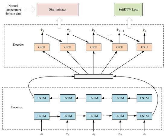
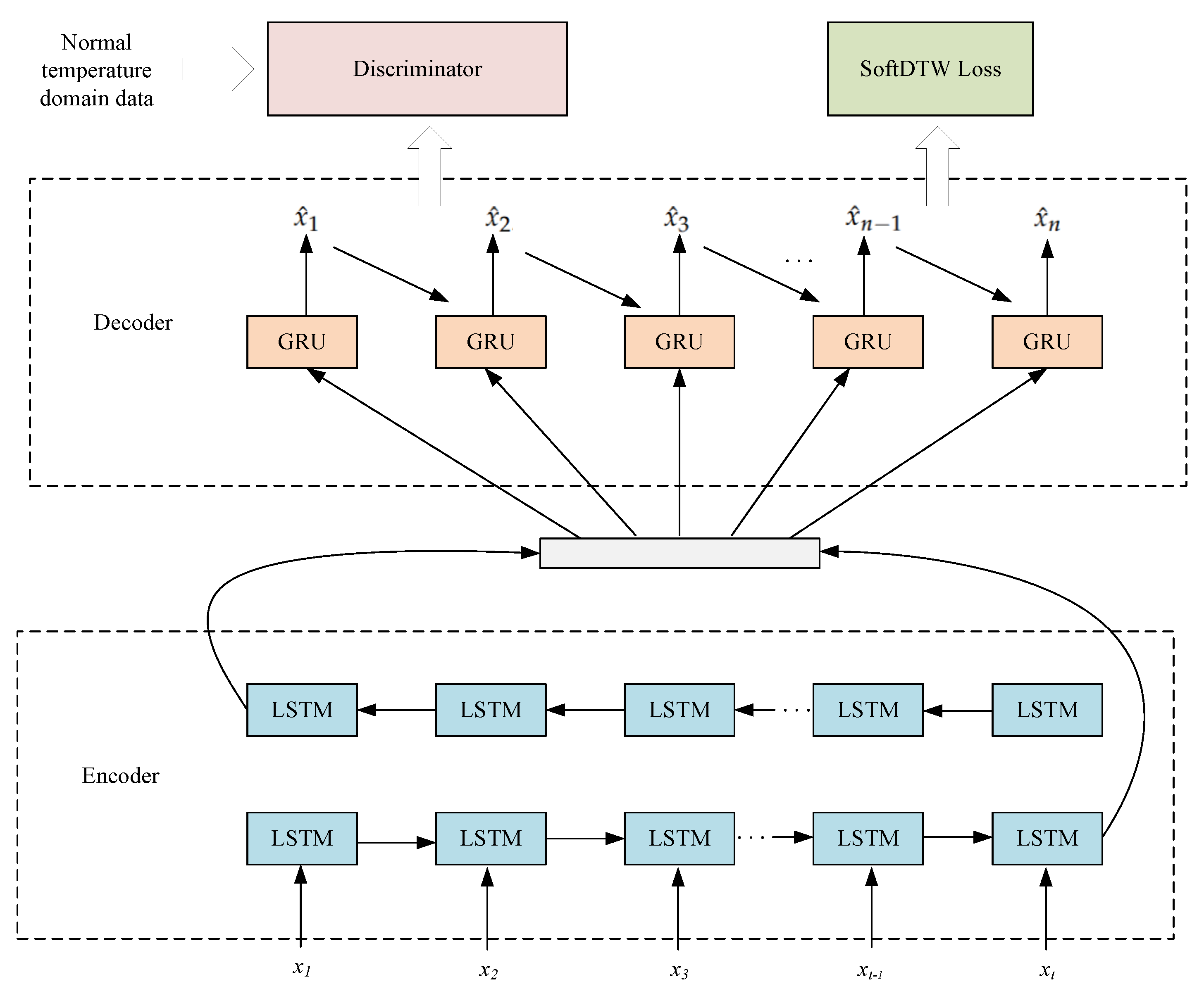
Due to cost and time constraints, the service life of computing systems is traditionally predicted by testing devices at elevated temperatures and extrapolating the results to normal operating and storage conditions. The distribution of degradation data differs across these conditions. To predict the degradation of critical parameters in aerospace-embedded computers across varying temperature regimes, we propose a cross-condition prediction model based on an encoder–decoder architecture with adversarial learning, as illustrated in Figure 2. Within a Generative Adversarial Network (GAN) framework, the model integrates Bidirectional Long Short-Term Memory (BiLSTM) networks and Gated Recurrent Units (GRU) to improve the alignment between generated and real sequences. It employs a soft dynamic time warping (soft-DTW) loss to align these sequences and reduce the distributional discrepancy between source (high-temperature) and target (normal-temperature) conditions, thereby enhancing the model’s generalization capability.
Figure 2.
Overall Network Architecture. This figure illustrates the proposed model’s GAN Framework, centered on three core components: a BiLSTM Encoder (feature extractor), a GRU Decoder (generator), and an LSTM Discriminator (discriminator). A Feature Mapping Layer is placed between the BiLSTM Encoder and GRU Decoder, converting the encoder’s extracted high-temperature features into decoder-compatible hidden states to support subsequent normal-temperature sequence generation. The input is the real high temperature sequence. The output is the generated low-temperature or normal temperature sequence converted from .
The proposed model comprises four key components: a BiLSTM encoder, a GRU decoder, an LSTM discriminator, and a Soft-DTW loss function. The BiLSTM encoder extracts features from the input high-temperature degradation data. The GRU decoder then uses these features to incrementally generate a normal-temperature degradation sequence. An LSTM-based discriminator evaluates the authenticity of the generated sequence. Finally, the Soft-DTW loss function provides flexible, elastic alignment of the generated degradation trends, ensuring accurate predictions across different thermal conditions.
3.2. Feature Encoder
The BiLSTM encoder functions as a feature extractor, capturing salient features from high-temperature degradation sequences. This module ingests time-series data on operational parameters and, by processing the data in both forward and backward directions, leverages BiLSTM capabilities to acquire comprehensive contextual information. The bidirectional structure enables the encoder to capture long-range temporal dependencies and preserve critical temporal relationships within the degradation data. The encoder’s input is the operational degradation sequence; its output includes both output states and hidden states, with the latter being passed to the GRU decoder to initialize the sequence generation process.
The BiLSTM-based feature extraction module consists of an input layer, bidirectional LSTM layers, and an output layer. The input layer receives the high-temperature degradation time-series data. The subsequent bidirectional LSTM layers contain forward and backward LSTM units that concurrently extract features from the sequence in both temporal directions. This process yields a rich feature representation that captures the temporal evolution of the degradation. Finally, the output layer consolidates these bidirectional features into multidimensional feature vectors for downstream processing.
3.3. Sequence Generator
In modeling the degradation of critical computer parameters, the GRU decoder acts as the sequence generator. It utilizes the hidden states from the BiLSTM encoder as its initial state to predict degradation trends through sequential generation. The GRU’s gated recurrent structure is adept at capturing dynamic temporal changes. This architecture inherently supports variable-length input and output sequences, accommodating the diverse lengths of degradation data encountered in practice. During training, the generator produces sequences of lengths determined by operational requirements, ensuring the accurate representation of degradation trends across different conditions. The encoder–decoder framework thus enables the generation of high-fidelity condition-specific degradation profiles.
The GRU-based sequence generation module transforms the feature vectors from the BiLSTM encoder into normal-temperature degradation time-series data. This module consists of an input layer, a GRU layer, and an output layer. The input layer receives the feature vectors. The GRU layer, with its gating mechanism, then regulates information flow to capture long-term temporal dependencies. Finally, the output layer produces the preliminary normal-temperature degradation sequence. The GRU’s efficient, streamlined architecture minimizes computational overhead while maintaining high performance, enabling rapid generation of high-quality sequences.
3.4. Sequence Discriminator
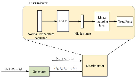
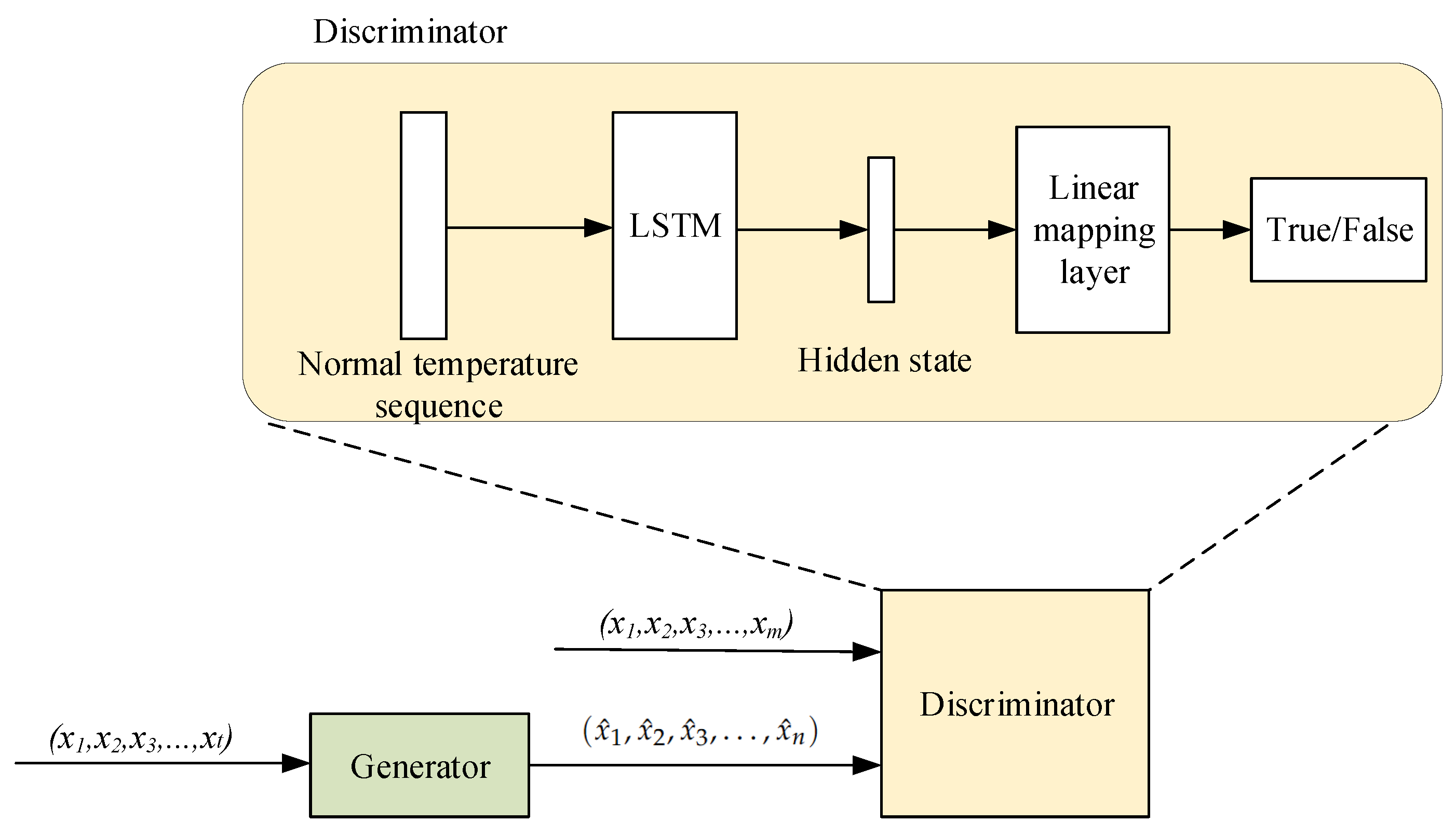
Within the adversarial training framework for critical parameter degradation, the generator and the LSTM-based discriminator collaborate to improve the quality and realism of generated sequences. The discriminator acts as an evaluator, analyzing the hidden states of input sequences to determine their authenticity relative to real degradation trends. As shown in the training framework (Figure 3), it is trained on both real degradation sequences (labeled as 1) and generated sequences (labeled as 0), with its parameters optimized using discrimination loss. This adversarial process not only sharpens the discriminator’s ability to identify synthetic data but also provides a learning signal that forces the generator to produce increasingly realistic sequences, thereby enhancing their cross-condition adaptability.
Figure 3.
Adversarial Sequence Discriminator. The generator produces a normal temperature sequence from real high temperature input sequence . The length of the normal-temperature time series is much longer than that of the high-temperature time series. This generated normal sequence and the real normal temperature time series are fed to the discriminator. The generated sequence length n may not be exactly the same as the real sequence length m. The discriminator processes the normal-temperature sequence to obtain a hidden state , then uses a linear mapping layer to output a binary result indicating whether the input sequence is real or fake, thereby implementing adversarial learning.
The discriminator, structured as a multilayer perceptron (MLP), processes both real and generated sequences. It extracts salient features to distinguish between them, outputting a probability that quantifies the perceived authenticity of each input sequence. This adversarial mechanism forces the generator to produce sequences that are increasingly indistinguishable from real data, thereby enhancing the model’s generalization capability. Through this iterative competition, the components ensure the output’s fidelity, with the discriminative feedback continuously guiding the generator’s optimization. This process enables the model to effectively generate realistic degradation trends across diverse operating conditions.
3.5. SoftDTW Calculation
Our approach innovatively integrates SoftDTW as a loss function to more effectively align generated and real degradation sequences across varying conditions. Unlike traditional mean squared error (MSE), which is inadequate for measuring similarity under dynamic time warping, SoftDTW provides a flexible similarity measure that accommodates sequences of varying lengths and temporal dynamics. As a differentiable metric, SoftDTW allows for the dynamic alignment of the generated sequence’s time axis with the target, enabling the model to learn optimal warping paths and produce more accurate degradation trends.
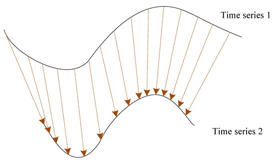
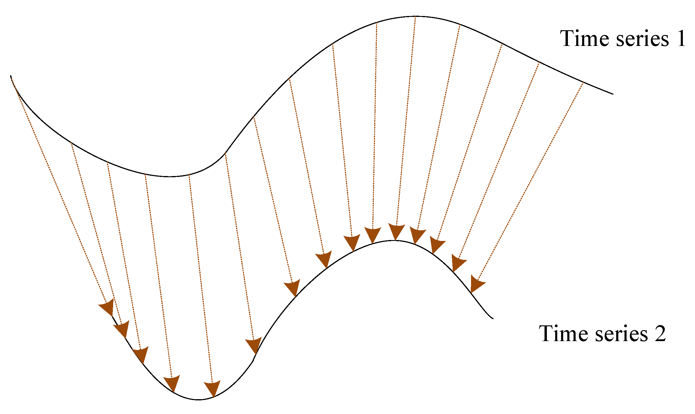
During training, the SoftDTW loss function dynamically aligns the generator’s output sequences with real degradation trends, computing a similarity distance between them. As shown in Figure 4, a lower loss value corresponds to a higher degree of similarity in both the trend and shape of the sequences. By effectively managing the complexities of time-series similarity across different conditions, SoftDTW improves the accuracy of the generated sequences. It also ensures that the generator maintains high alignment quality as it dynamically refines its generation strategy.
Figure 4.
Soft dynamic time Warping. This figure visually demonstrates the Soft DTW algorithm. It illustrates the process of aligning two time series, “Time series 1” and “Time series 2”, by showing the mapping connections (lines with arrows) between corresponding points in the two series. Through this alignment, Soft DTW can measure the similarity between the two time series in a flexible manner, accommodating differences in their temporal dynamics and lengths.
Soft-DTW, a differentiable variant of Dynamic Time Warping, addresses the challenge of aligning time series with different lengths by introducing a soft-minimum operation, as illustrated in Algorithm 1. This provides the flexibility to align sequences of unequal length, mitigating excessive warping and potential information loss associated with hard alignment in traditional DTW, particularly for long sequences. Furthermore, by averaging alignment paths with weights, Soft-DTW exhibits greater robustness to noise and outliers, resulting in more accurate and stable alignments. Its key advantage for deep learning is differentiability, which enables seamless integration into end-to-end training models.
| Algorithm 1 Algorithm Steps of Soft-DTW. |
|
3.6. Loss Functions of Total Network
We design three core loss functions and integrate them into an adversarial training framework, as detailed below. Here, denotes the distribution of real data. z is the noise input to the generator G, and denotes the distribution of this input noise. N is the batch size. BCE(.,. ) represents the binary cross-entropy function.
- Discriminator Loss () quantifies the discriminator’s ability to distinguish real samples () from generated samples ( where ) using binary cross-entropy loss for discriminator optimization:Here, outputs a probability in (1 = real, 0 = false).
- Generator Loss () guides the generator to produce realistic samples by “fooling” the discriminator for generator optimization:
- Soft-DTW Alignment Loss () Enforces temporal trend consistency between generated and real sequences via elastic alignment:where and are the i-th generated and real samples, N is batch size, and denotes the differentiable alignment distance.
- Overall Training Loss () The model uses alternating adversarial optimization. Generator (G) minimizes to improve realism. Discriminator (D) maximizes to enhance distinguishability. is minimized to ensure temporal alignment.
The adversarial training process employs an iterative, alternating optimization strategy. Within each epoch, the discriminator is first trained to enhance its ability to differentiate between real and generated sequences by minimizing its classification loss. Subsequently, with the discriminator’s parameters fixed, the generator is trained using a composite loss function. This function combines an adversarial loss, which encourages the generator to fool the discriminator, with a SoftDTW loss that directly enforces temporal consistency between the generated and real sequences. This dual-objective approach ensures the co-optimization of distributional matching and structural fidelity. Consequently, the model not only leverages the GAN’s power to learn complex data distributions but also incorporates structural constraints to ensure temporal realism, achieving both high authenticity and accuracy in generating complex degradation sequences. The training process of the overall network is illustrated in Algorithm 2.
| Algorithm 2 Overall Training Framework. |
|
The proposed network architecture offers substantial advantages for predicting the degradation of critical computer parameters. Its adversarial training framework significantly enhances generalization, enabling the generation of highly realistic sequences. The BiLSTM encoder provides a robust foundation by extracting comprehensive features from high-temperature sequences. Subsequently, the GRU decoder leverages these features to efficiently generate high-quality normal-temperature degradation sequences while capturing long-term temporal dependencies. Finally, the Soft-DTW loss function ensures precise alignment between the generated and real sequences, effectively accommodating variations in sequence length and dynamics.
4. Experiments
4.1. Datasets
Different electronic systems are defined by distinct key characteristics. For a meaningful health assessment, these characteristics must accurately reflect the system’s operational state. This study uses the embedded computer—the core processing unit of equipment electronic systems—as a case study to illustrate the selection of key characteristics. The selected parameters must capture the reliability requirements across various operating conditions, thereby providing a comprehensive and scientifically valid representation of the computer’s health status.
The selection of key parameters for embedded computers follows several criteria. First, parameters should be as independent as possible to minimize mutual interference. Second, they must be directly measurable or statistically quantifiable to allow for objective comparison. Finally, the chosen parameters must collectively reflect the overall degradation trend of the electronic system.
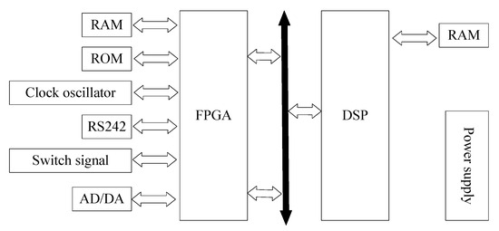
Through a simplified analysis of the electronic system (Figure 5), the following key characteristic parameters, which significantly contribute to the overall system degradation, have been identified:
Figure 5.
Embedded computer architecture diagram. The diagram illustrates the embedded system architecture, consisting of two core processors (FPGA for reconfigurable parallel processing and DSP for high-efficiency digital signal operations) with high-speed bidirectional communication. It integrates FPGA-coupled RAM/ROM, DSP-associated RAM, FPGA-connected external interfaces (clock oscillator, RS242, switch signal module, AD/DA converter), and a power supply module.
- Clock Oscillator: The minimal flight control computer system consists primarily of DSP, FPGA, reset, memory, and clock circuits. Experimental results indicate that the clock oscillator demonstrates a more pronounced degradation trend than other components. As the primary time reference for the entire system, its degradation directly impacts operational timing accuracy.
- Analog Signal Conversion (AD/DA): This category includes analog-to-digital (AD) acquisition and digital-to-analog (DA) conversion. Data from natural storage, accelerated aging tests, and returned product overhauls consistently show that analog signal parameters degrade significantly with increased storage time.
- Optocoupler and Baud Rate: Using differential RS422 communication as an example, the transmitter employs a differential driver while the receiver uses an optocoupler for isolated signal reception. Parameter drift in the optocoupler and degradation of the interface oscillator directly affect the communication waveform’s baud rate. This can cause timing errors that lead to communication data exceeding acceptable error limits.
The experimental dataset for this study comprises time-series data recorded under high- and low-temperature conditions for three key component types associated with system degradation: the clock oscillator, analog signal module, and optocoupler communication module. For each component type and temperature condition, approximately 200 time series were collected. Parameter measurements were documented daily to track the progression of degradation.
During high-temperature testing, the electronic units were maintained in a de-energized state. Power-on tests were conducted at 48-hour intervals during pauses in the high-temperature exposure. Before each test, the units were stabilized to laboratory ambient temperature. Each test was repeated three times, and the average value was calculated to ensure data reliability and repeatability. Following each power-on test, the units were returned to the high-temperature environment to resume the degradation experiment.
To enhance model generalization and mitigate the limitations of a small sample size, the dataset underwent two standardized preprocessing steps: normalization and Gaussian noise injection. Normalization unified the parameter scales to eliminate magnitude-related bias, while noise injection simulated minor real-world fluctuations to improve dataset robustness. This preprocessing provided a rigorous foundation for training the proposed network and analyzing the degradation sequences of the target components.
The dataset was partitioned into training and test sets with an 80:20 ratio. From an architectural perspective, the high-temperature time series is fed into the encoder as a complete sequence. The decoder is designed to output the corresponding low-temperature sequence. In practice, the encoder–decoder model generates the low-temperature series iteratively in segments, which are subsequently concatenated to form the final, complete output sequence.
In the experiments, the model utilizes high-temperature degradation sequences to predict the long-term degradation trends of the key parameters for the specified aerospace computer under normal ambient temperature conditions.
4.2. Implementation Details
The experiments were conducted using PyTorch 2.0.1 on a Python 3.8 platform, with an NVIDIA V100 GPU (32 GB memory). The model’s hyperparameters were configured as follows: a batch size of 64, an input feature dimension of 1, a hidden layer dimension of 32, three layers for each LSTM and GRU module, and 800 training epochs. Both the generator and discriminator were optimized using Adam, with the learning rate scheduled to decay sequentially from 0.01 to 0.0001. For the Soft-DTW loss function, the smoothing and scaling parameters were set to and , respectively.
Several data preprocessing and training strategies were employed. Time-series data were augmented through translation, scaling, noise injection, and resampling. Data normalization and differencing of raw data were applied to scale and desensitize. Training used a sliding window spanning half the sequence length. To ensure stable GAN training, the discriminator and generator were updated with separate gradient steps, and gradient clipping was applied to constrain parameter updates and accelerate convergence.
The generator and discriminator networks were designed with relatively simple architectures to effectively control computational overhead. This design reduces resource consumption during training and enables efficient inference. Notably, the model can perform inference on a standard CPU, eliminating a strict dependency on high-performance GPUs and enhancing its practical deployment potential.
4.3. Experiment Metric
In time series forecasting, the difference between predicted and actual values is typically evaluated using Mean Squared Error (MSE) and Mean Absolute Error (MAE). The formulas for these metrics are presented below, where N represents the number of prediction steps, denotes the ground truth, and represents the predicted value.
4.4. Experiment Result
This study investigates the mapping between high- and low-temperature degradation data in embedded computers, employing deep learning to predict and simulate the degradation behavior of critical components, including optocouplers, digital-to-analog converters, and crystal oscillators. The problem is addressed from two complementary perspectives: time-series forecasting and data generation. For forecasting, we used sequence models such as Long Short-Term Memory (LSTM) networks and Transformers to predict future room-temperature degradation from historical data, capturing temporal dependencies to extrapolate system performance across conditions. For data generation, we formulated the task as synthesizing realistic degradation sequences under varying scenarios. Sequence-to-sequence (Seq2Seq) models and their variants excelled in this capacity, leveraging encoder–decoder architectures and attention mechanisms to generate plausible sequences by dynamically focusing on critical input features, thereby enhancing the fidelity and reliability of the synthetic data.
We benchmarked our approach against leading methods from recent years for predicting the room-temperature degradation of mission-critical optocouplers, digital-to-analog converters, and crystal oscillators. As shown in Table 1, our method demonstrates consistently and markedly superior performance.
Table 1.
Degradation experiment results.
As summarized in Table 1, our method consistently achieves superior accuracy across all datasets compared to previous state-of-the-art models. This performance gain is largely attributable to the integration of transfer learning and adversarial training, which facilitates distribution alignment between the iteratively predicted sequences and the actual data. This alignment effectively mitigates the accumulation of prediction errors common in long-horizon forecasting. Overall, our approach outperforms benchmark models, including LSTM, Transformer, and standard Seq2Seq architectures, demonstrating its robustness and effectiveness in capturing complex degradation dynamics. These results underscore the efficacy of our method in accurately modeling degradation behavior, offering a more reliable predictive solution for embedded computer systems.
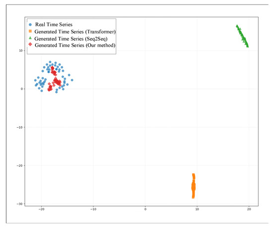
For a comprehensive comparison, we selected representative models from two dominant paradigms in time-series analysis: deep learning-based forecasting, exemplified by the Transformer, and sequence generation based on the Seq2Seq architecture. The t-SNE visualization in Figure 6 compares real normal-temperature data with data generated from 160 °C sequences using different methods. The data produced by our model form a tight cluster with the real data in the embedded space, with distributions that are highly similar. In contrast, the data generated by other methods, such as the Transformer and Seq2Seq, are distinctly separated from the real data. This provides direct visual evidence that our method achieves a significantly superior alignment of feature distributions.
Figure 6.
T-SNE visualization for feature assignment. The data points from the normal-temperature time series generated by our method are tightly clustered with this cluster of real normal-temperature data, showing a highly similar spatial distribution. In contrast, the data points of the normal-temperature time series generated by other methods have a clear spatial gap between their respective clusters and the real data cluster, indicating a lack of effective feature alignment with the real normal-temperature data.
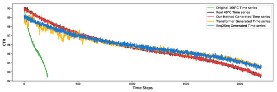
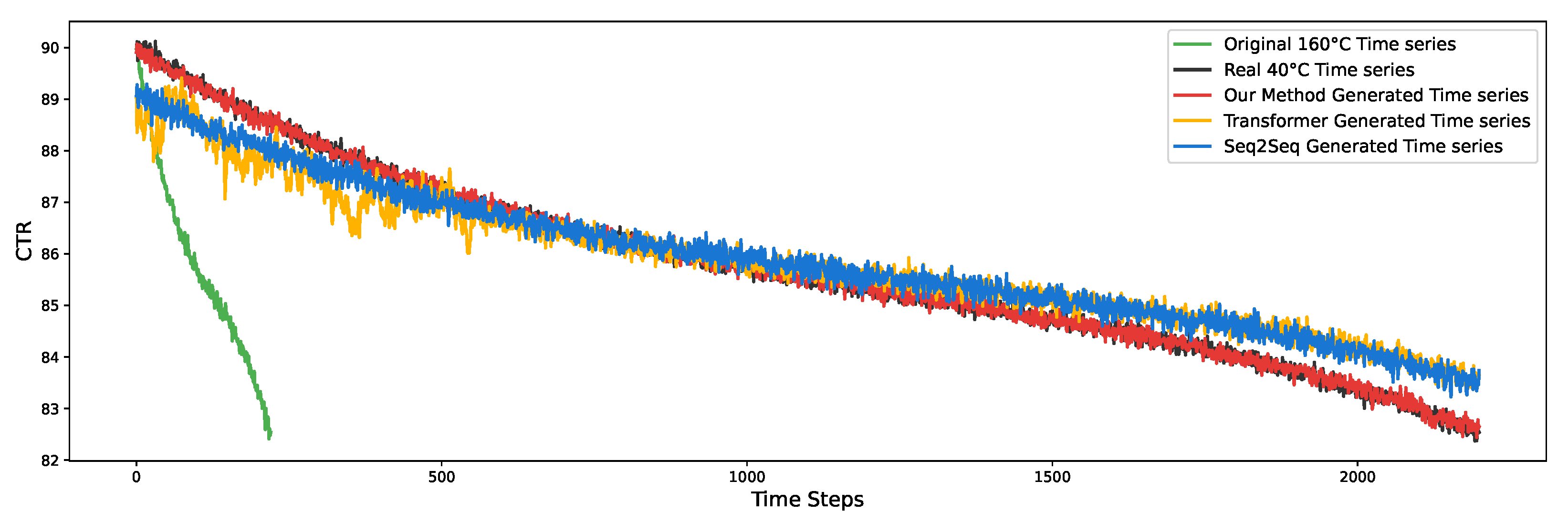
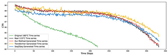
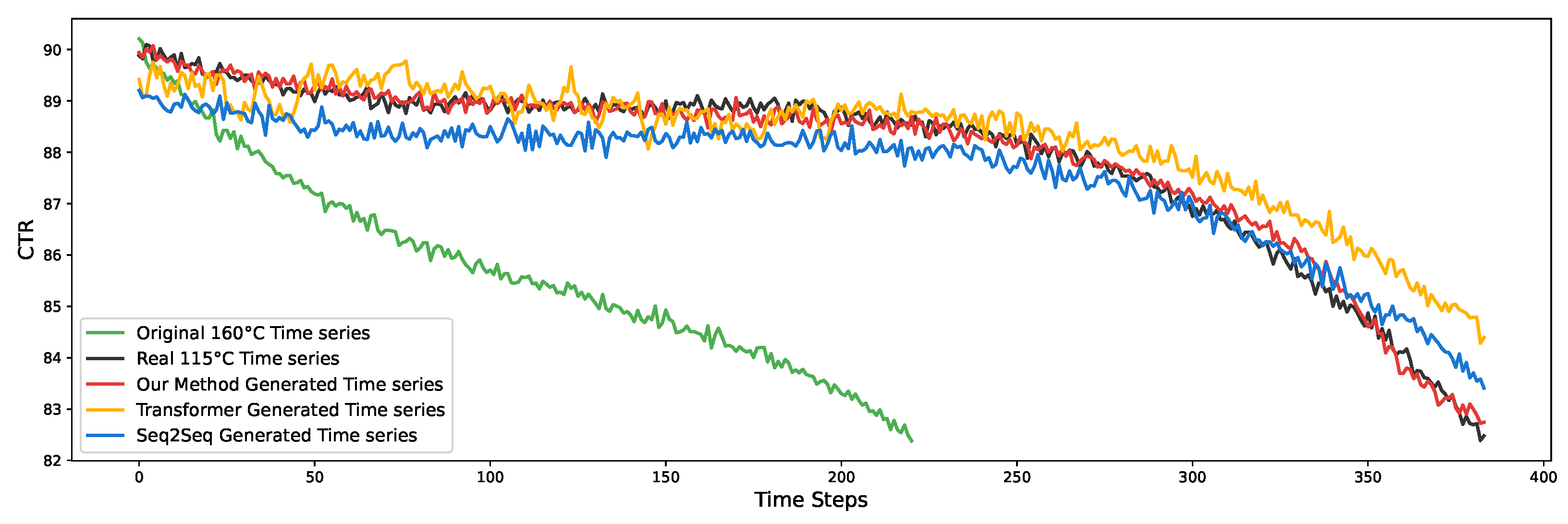
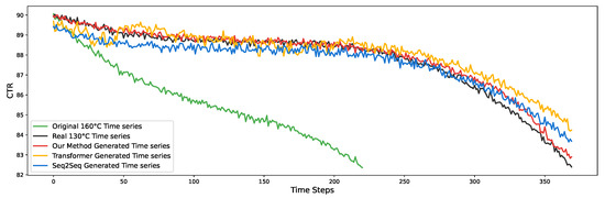
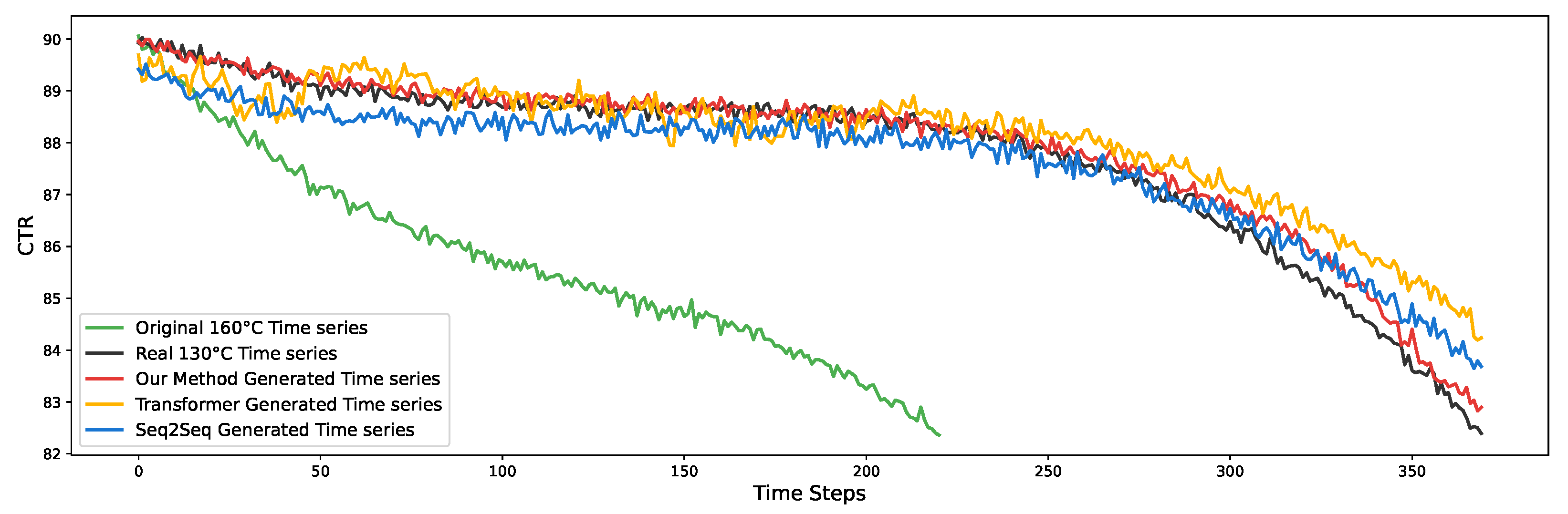
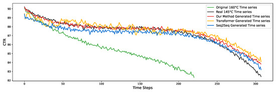
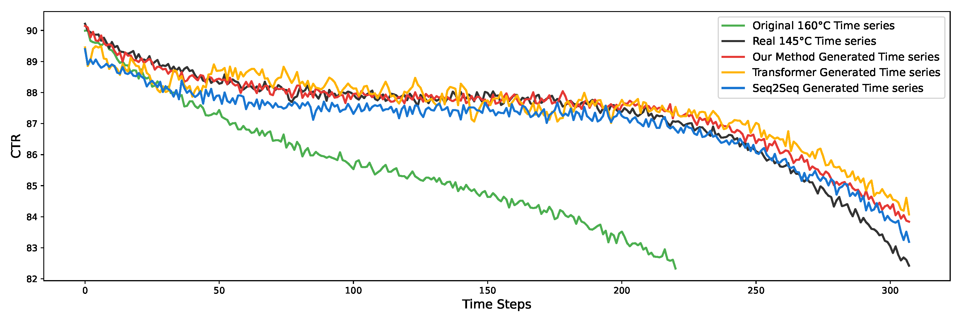
Our study introduces a novel method for generating degradation data for optocouplers across different temperature conditions. The visual results in Figure 7, Figure 8, Figure 9 and Figure 10 demonstrate the efficacy of this approach, successfully illustrating the generated degradation trends at various temperatures. The observed patterns are consistent and physically meaningful, confirming the robustness and accuracy of our method. These visualizations highlight distinct degradation behaviors under different thermal stresses and underscore our model’s capability to accurately capture and replicate these dynamics. This is crucial for assessing the performance and reliability of optocouplers in diverse operational environments. In computer degradation, higher temperatures typically result in shorter degradation experiment durations. In contrast, lower temperatures demand longer degradation periods to achieve an equivalent degree of aging. Consequently, there are differences in the axes and units of the corresponding time series in Figure 7, Figure 8, Figure 9 and Figure 10.
Figure 8.
Optocoupling degradation mapped from 160 °C to 115 °C.
Figure 9.
Optocoupling degradation mapped from 160 °C to 130 °C.
Figure 10.
Optocoupling degradation mapped from 160 °C to 145 °C.
The superior performance of the proposed method can be attributed to three key factors. First, the adversarial learning component compels the model to extract generalizable features that are robust to specific operational conditions. This prevents the generated sequences from deviating from the underlying physical degradation rules of the target scenario, a capability lacking in baseline methods without adversarial mechanisms. Second, the Soft-DTW loss function effectively addresses temporal alignment challenges by focusing on overall trend similarity through flexible elastic matching, thereby avoiding over-sensitivity to point-to-point deviations or excessive sequence warping. Third, these components work synergistically: the condition-invariant features from adversarial learning are further refined by Soft-DTW to align with the temporal dynamics of the target domain. This combined effect surpasses the performance of either component used in isolation, effectively compensating for the baseline methods’ shortcomings in scenario adaptation and temporal alignment.
Prediction errors at each time point, calculated from multiple measurements relative to the actual values, exhibited a normal distribution with minimal variance. Utilizing the Mean Squared Error (MSE) presented in Table 1, the standard deviation of prediction errors was derived as the square root of the MSE. Correspondingly, the 95% confidence interval for the predicted mean at each time point was computed as the predicted mean ±1.96 × the standard deviation of the error. The vast majority of the predicted values fell within their respective 95% confidence intervals, demonstrating high consistency and statistical reliability of the prediction outcomes.
4.5. Ablation Studies
In this study, to assess the impact of two enhancements, Adversarial Learning (A) and Soft Dynamic Time Warping (D), on model performance, we conducted a series of ablation experiments. The results of these experiments, detailed in Table 2, demonstrate the incremental improvements in model performance as each enhancement is introduced. Specifically, the individual implementation of Adversarial Learning (A) and Soft Dynamic Time Warping (D) provides noticeable gains, while their combination yields the most substantial enhancement. This indicates that integrating A and D not only enhances the model’s accuracy and robustness but also optimizes its overall efficiency in handling complex data sequences. The findings underscore the effectiveness of these enhancements and their potential to significantly advance the model’s capabilities in practical applications.
Table 2.
Ablation experiment results.
To compare the performance of different components, we conducted ablation experiments by substituting alternative modules: specifically, we replaced the BiLSTM with a GRU as the encoder (denoted as Module (GRU)), and replaced the Soft-DTW with standard DTW and MSE respectively (denoted as Module (DTW) and Module (MSE)), as shown in Table 3.
Table 3.
Ablation different components experiment results.
5. Conclusions
This study addresses a critical challenge in embedded computer system reliability: the limited correlation between high-temperature accelerated test data and normal-temperature degradation trends—a common bottleneck due to time and cost constraints in traditional testing. To solve this, we propose a method that combines adversarial learning and soft DTW. Adversarial learning enables cross-temperature feature transfer, extracting domain-invariant features to generate normal-temperature degradation sequences from high-temperature data; soft DTW further improves accuracy by aligning the generated sequences with real normal-temperature sequences, mitigating errors caused by nonlinear temporal variations. Experimental results confirm that our method outperforms conventional approaches in predicting embedded computer degradation. It provides a more reliable solution for degradation analysis and lifespan estimation, ultimately enhancing the reliability of embedded computational systems.
While this study provides valuable insights into the prediction of embedded system degradation, it is subject to several limitations. The current experimental framework is constrained to thermal stress testing, excluding other critical factors such as electromagnetic radiation and voltage fluctuations. Furthermore, the model is trained and validated on a laboratory dataset augmented with synthesized data, which may not fully capture the complexity of real-world operational environments, potentially limiting its field generalizability. Future research will focus on two primary directions: first, validating the model’s real-world adaptability by incorporating on-orbit satellite data; and second, extending the framework into a multi-stress model that concurrently integrates temperature, radiation, and electrical stressors. These advancements will enhance the model’s robustness and practical utility for engineering-oriented degradation analysis and lifespan estimation.
Author Contributions
Y.M.: Conceptualization, Methodology, Software, Formal analysis, Writing. Y.L.: Data curation, Resources. X.L.: Supervision. P.H.: funding acquisition. L.L.: Project administration. B.C.: Conceptualization. Y.Z.: software, validation. X.H.: data curation, software, validation. All authors have read and agreed to the published version of the manuscript.
Funding
This work was supported by a confidential research project. Due to the classified nature of the funding source, specific grant details cannot be disclosed.
Data Availability Statement
The datasets presented in this article are not readily available due to technical limitations and commercial restrictions. Requests to access the datasets should be directed to the corresponding author (Yuanhong Mao, email: yuanhongmao@hotmail.com).
Conflicts of Interest
The authors declare no conflict of interest.
Abbreviations
The following abbreviations are used in this manuscript:
| CTR | Current Transfer Ratio |
| CNN | Convolutional Neural Network |
| RNN | Recurrent Neural Network |
| LSTM | Long Short-Term Memory |
| GRU | Gate Recurrent Unit |
| DTW | Dynamic Time Warping |
| GAN | Generative Adversarial Network |
| BiLSTM | Bidirectional Long Short-term Memory |
References
- Mao, Y.; Chai, B.; Liu, X.; Li, L.; Tian, W. A Review of Research on Intelligent Health Management Technologies for Electronic Systems. Microelectron. Comput. 2025, 42, 37–53. [Google Scholar] [CrossRef]
- Qin, R.; Guo, D.; Li, Q.; Zhang, A.; Liu, X.; Xu, K.D. Millimeter-Wave Bandpass Filter Using Rectangular Waveguide and SSPP With a Notched Band. IEEE Photon. Technol. Lett. 2025, 37, 29–32. [Google Scholar] [CrossRef] [Scilit]
- Mao, Y.; Ma, Z.; Gao, S.; Li, L.; Yuan, B.; Chai, B.; He, P.; Liu, X. A Method of Embedded Computer Degradation Trend Prediction. In Proceedings of the 2022 5th International Conference on Pattern Recognition and Artificial Intelligence (PRAI), Chengdu, China, 19–21 August 2022; pp. 1338–1343. [Google Scholar] [CrossRef] [Scilit]
- Kim, Y. Convolutional Neural Networks for Sentence Classification. arXiv 2014, arXiv:1408.5882. [Google Scholar] [CrossRef] [Scilit]
- Hochreiter, S.; Schmidhuber, J. Long short-term memory. Neural Comput. 1997, 9, 1735–1780. [Google Scholar] [CrossRef] [Scilit] [PubMed]
- Chung, J.; Gulcehre, C.; Cho, K.; Bengio, Y. Empirical Evaluation of Gated Recurrent Neural Networks on Sequence Modeling. arXiv 2014, arXiv:1412.3555. [Google Scholar] [CrossRef] [Scilit]
- Zhang, S.; Zheng, D.; Hu, X.; Yang, M. Bidirectional Long Short-Term Memory Networks for Relation Classification. In Proceedings of the 29th Pacific Asia Conference on Language, Information and Computation, Shanghai, China, 30 October–1 November 2015; pp. 73–78. [Google Scholar]
- Subakan, C.; Ravanelli, M.; Cornell, S.; Bronzi, M.; Zhong, J. Attention is all you need in speech separation. In Proceedings of the ICASSP 2021—2021 IEEE International Conference on Acoustics, Speech and Signal Processing (ICASSP), Toronto, ON, Canada, 6–11 June 2021; pp. 21–25. [Google Scholar]
- Osterman, M. We Still Have a Headache With Arrhenius. Electron. Cool. 2001, 7, 53–55. [Google Scholar]
- Wilcoxon, R. Does a 10 °C Increase in Temperature Really Reduce the Life of Electronics by Half? IEEE Trans. Device Mater. Reliab. 2017, 17, 1120–1131. [Google Scholar]
- Zhang, Q.; Cui, N.; Shang, Y.; Duan, B.; Zhang, C. Arrhenius Equation-Based Model to Predict Lithium-Ions Batteries’ Performance. Energies 2022, 15, 3542. [Google Scholar] [CrossRef] [Scilit]
- Lele, S.; Arora, A.; Benson, K. Predicting the Life of Li-Ion Batteries Using the Arrhenius Model; White paper; Vertiv: Phoenix, AZ, USA; Chicago, IL, USA, 2018. [Google Scholar]
- Li, X.; Song, Z.-T.; Cai, D.-L.; Chen, X.-G.; Jia, X.-L. An SPICE Model for PCM Based on Arrhenius Equation. Chin. Phys. Lett. 2009, 26, 128501. [Google Scholar] [CrossRef] [Scilit]
- Kuehl, R.W. Stability of thin film resistors—Prediction and differences base on time-dependent Arrhenius law. Microelectron. Reliab. 2009, 49, 51–58. [Google Scholar] [CrossRef] [Scilit]
- Bartnikas, R.; Morin, R. Multi-stress aging of stator bars with electrical, thermal, and mechanical stresses as simultaneous acceleration factors. IEEE Trans. Energy Convers. 2004, 19, 702–714. [Google Scholar] [CrossRef]
- Yu, H.; Yuan, S.; Chang, W.; Gong, Y. Lifetime Prediction and Stability Analysis of TMR Chips Based on a Modified Arrhenius-Eyring Model. In Proceedings of the 2025 4th International Conference on Electronics, Integrated Circuits and Communication Technology (EICCT), Chengdu, China, 11–13 July 2025; pp. 587–591. [Google Scholar] [CrossRef] [Scilit]
- Zhang, F.; Tian, R.; Wang, P.; Dong, L. Multi-stress accelerated life evaluation method considering generalized coupling. Syst. Eng. Electron. 2023, 45, 3350. [Google Scholar] [CrossRef]
- Qian, R.; Yang, L.; Gou, L. Multiple Physical Field Coupling Modeling and Failure Effect Analysis of Aero-Engine VSV Actuating System. Proc. Mech. Eng. Technol. 2022, 11, 14. [Google Scholar] [CrossRef]
- Mao, Y.; Sun, C.; Xu, L.; Liu, X.; Chai, B.; He, P. A survey of time series forecasting methods based on deep learning. Microelectron. Comput. 2023, 40, 8–17. [Google Scholar] [CrossRef]
- Wang, S.; Lin, R.; Bao, L.; Xue, N.; Li, H. Capacitor Capacitance Prediction Method Based on Time Series Method. In Proceedings of the 2024 International Conference on Advances in Electrical Engineering and Computer Applications (AEECA), Dalian, China, 16–18 August 2024; pp. 75–80. [Google Scholar]
- Gorlov, M.; Strogonov, A.; Smirnov, D.Y. Transistor-degradation prediction by time-series analysis. Russ. Microelectron. 2006, 35, 337–344. [Google Scholar] [CrossRef] [Scilit]
- Amini, M.H.; Kargarian, A.; Karabasoglu, O. ARIMA-based decoupled time series forecasting of electric vehicle charging demand for stochastic power system operation. Electr. Power Syst. Res. 2016, 140, 378–390. [Google Scholar] [CrossRef] [Scilit]
- Meng, J.; Yue, M.; Diallo, D. A degradation empirical-model-free battery end-of-life prediction framework based on Gaussian process regression and Kalman filter. IEEE Trans. Transp. Electrif. 2022, 9, 4898–4908. [Google Scholar] [CrossRef] [Scilit]
- Ni, J.; Zhang, C.; Zhang, X.; Lei, T. Remaining useful life prediction method for mosfet based on time series model. In Proceedings of the 2021 IEEE Asia-Pacific Conference on Image Processing, Electronics and Computers (IPEC), Dalian, China, 14–16 April 2021; pp. 1217–1221. [Google Scholar]
- Yin, Y.; Chen, R.; Thukral, V.; He, C.; Li, P. Reliable Board-Level Degradation Prediction with Monotonic Segmented Regression under Noisy Measurement. In Proceedings of the 2025 IEEE 43rd VLSI Test Symposium (VTS), Tempe, AZ, USA, 28–30 April 2025; pp. 1–7. [Google Scholar]
- Elman, J.L. Finding Structure in Time. Cogn. Sci. 1990, 14, 179–211. [Google Scholar] [CrossRef]
- Kiranyaz, S.; Avci, O.; Abdeljaber, T.; Ince, T.; Gabbouj, M.; Inman, D.J. 1D convolutional neural networks and applications: A survey. Mech. Syst. Signal Process. 2021, 151, 107398. [Google Scholar] [CrossRef] [Scilit]
- Chen, X.; Yang, Y.; Sun, J.; Deng, Y.; Yuan, Y. A novel time series forecasting model for capacity degradation path prediction of lithium-ion battery pack. J. Supercomput. 2024, 80, 10959–10984. [Google Scholar] [CrossRef] [Scilit]
- Singh, S.; Budarapu, P. Deep machine learning approaches for battery health monitoring. Energy 2024, 300, 131540. [Google Scholar] [CrossRef] [Scilit]
- Gao, L.; Liu, C.; Xiao, Y.; Qi, C.; Huo, M. Remaining Useful Life Prediction of Power Electronic Devices with Physics-Informed Deep Learning and Sparse Data. IEEE Trans. Power Electron. 2025, 40, 16068–16073. [Google Scholar] [CrossRef] [Scilit]
- Mao, Y.; Hu, X.; Xu, Y.; Zhang, Y.; Li, Y.; Lu, Z.; Miao, Q. Decomposition-Aware Framework for Probabilistic and Flexible Time Series Forecasting in Aerospace Electronic Systems. Mathematics 2025, 13, 262. [Google Scholar] [CrossRef] [Scilit]
- Mao, Y.; Ma, Z.; Liu, X.; He, P.; Chai, B. A Long-Term Prediction Method of Computer Parameter Degradation Based on Curriculum Learning and Transfer Learning. Mathematics 2023, 11, 3098. [Google Scholar] [CrossRef] [Scilit]
- Goodfellow, I.J.; Pouget-Abadie, J.; Mirza, M.; Xu, B.; Warde-Farley, D.; Ozair, S.; Courville, A.; Bengio, Y. Generative Adversarial Networks. In Proceedings of the Advances in Neural Information Processing Systems (NIPS), Montreal, QC, Canada, 8–13 December 2014; pp. 2672–2680. [Google Scholar]
- Yoon, J.; Jarrett, D.; van der Schaar, M. Time-series generative adversarial networks. In Proceedings of the 33rd International Conference on Neural Information Processing Systems, Vancouver, BC, Canada, 8–14 December 2019; pp. 5508–5518. [Google Scholar]
- Ahmed, N.; Schmidt-Thieme, L. Sparse self-attention guided generative adversarial networks for time-series generation. Int. J. Data Sci. Anal. 2023, 16, 421–434. [Google Scholar] [CrossRef] [Scilit]
- EskandariNasab, M.; Hamdi, S.M.; Boubrahimi, S.F. Seriesgan: Time series generation via adversarial and autoregressive learning. In Proceedings of the 2024 IEEE International Conference on Big Data (BigData), Washington, DC, USA, 15–18 December 2024; pp. 860–869. [Google Scholar]
- Zhou, H.; Zhang, S.; Peng, J.; Zhang, S.; Li, J.; Xiong, H.; Zhang, W. Informer: Beyond Efficient Transformer for Long Sequence Time-Series Forecasting. Proc. AAAI Conf. Artif. Intell. 2021, 35, 11106–11115. [Google Scholar] [CrossRef] [Scilit]
- Lai, G.; Chang, W.C.; Yang, Y.; Liu, H. Modeling Long- and Short-Term Temporal Patterns with Deep Neural Networks. In Proceedings of the 41st Annual International ACM SIGIR Conference on Research and Development in Information Retrieval (SIGIR), Ann Arbor, MI, USA, 8–12 July 2018; pp. 95–104. [Google Scholar] [CrossRef] [Scilit]
- Wu, H.; Xu, J.; Wang, J.; Long, M. Autoformer: Decomposition Transformers with Auto-Correlation for Long-Term Series Forecasting. In Proceedings of the 35th Conference on Neural Information Processing Systems (NeurIPS), Electr Network, Online, 6–14 December 2021; Volume 34. [Google Scholar]
- Kitaev, N.; Kaiser, Ł.; Levskaya, A. Reformer: The efficient transformer. arXiv 2020, arXiv:2001.04451. [Google Scholar] [CrossRef] [Scilit]
- Liu, Y.; Hu, T.; Zhang, H.; Wu, H.; Wang, S.; Ma, L.; Long, M. iTransformer: Inverted Transformers Are Effective for Time Series Forecasting. In Proceedings of the Twelfth International Conference on Learning Representations, Vienna, Austria, 7–11 May 2024. [Google Scholar]
- Sutskever, I.; Vinyals, O.; Le, Q.V. Sequence to Sequence Learning with Neural Networks. In Proceedings of the Advances in Neural Information Processing Systems, New Orleans, LA, USA, 10–16 December 2014; Ghahramani, Z., Welling, M., Cortes, C., Lawrence, N., Weinberger, K., Eds.; Curran Associates, Inc.: Red Hook, NY, USA, 2014; Volume 27. [Google Scholar]
- Lu, O.H. A Seq2Seq transformation strategy for generalizing a pre-trained model in anomaly detection of rolling element bearings. Expert Syst. Appl. 2024, 254, 124297. [Google Scholar] [CrossRef] [Scilit]

Disclaimer/Publisher’s Note: The statements, opinions and data contained in all publications are solely those of the individual author(s) and contributor(s) and not of MDPI and/or the editor(s). MDPI and/or the editor(s) disclaim responsibility for any injury to people or property resulting from any ideas, methods, instructions or products referred to in the content. |
© 2025 by the authors. Licensee MDPI, Basel, Switzerland. This article is an open access article distributed under the terms and conditions of the Creative Commons Attribution (CC BY) license (https://creativecommons.org/licenses/by/4.0/).