Mathematical Properties of the Inverted Topp–Leone Family of Distributions

Abstract

This article defines an inverted Topp–Leone distribution. Several mathematical properties and maximum likelihood estimation of parameters of this distribution are considered. The shape of the distribution for different sets of parameters is discussed. Several mathematical properties such as the cumulative distribution function, mode, moment-generating function, survival function, hazard rate function, stress-strength reliability R, moments, Rényi entropy, Shannon entropy, Fisher information matrix, and partial ordering associated with this distribution, have been derived. Distributions of the sum and quotient of two independent inverted Topp–Leone variables have also been obtained.

1. Introduction

A random variable X is said to have a Topp–Leone distribution, denoted by $X\sim TL(\nu ;\sigma )$, if its PDF is given by

$$f_{\mathrm{T}\mathrm{L}}(x;\nu ,\sigma )={\displaystyle \frac{2\nu }{\sigma }}{\left({\displaystyle \frac{x}{\sigma }}\right)}^{\nu -1}\left(1-{\displaystyle \frac{x}{\sigma }}\right){\left(2-{\displaystyle \frac{x}{\sigma }}\right)}^{\nu -1},0<x<\sigma <\infty .$$

(1)

For $0<\nu <1$, the distribution defined by the density of Equation (1) is referred to as the J-shaped distribution by Topp and Leone [1] because $f(x;\nu ,\sigma )>0$, $f^{\prime }(x;\nu ,\sigma )<0$ and $f^{\prime \prime }(x;\nu ,\sigma )>0$ for all $0<x<\sigma$, where $f^{\prime }(x;\nu ,\sigma )$ and $f^{\prime \prime }(x;\nu ,\sigma )$ are the first and the second derivatives, respectively, of $f(x;\nu ,\sigma )$. For $\nu >1$, Equation (1) attains different shapes depending on values of parameters (see Kotz and van Dorp [2]). This family has a close affinity to the family of beta distributions, as the distribution of $1-X/\sigma$ has a McDonald beta distribution (Kumaraswamy distribution with parameters 2 and $\nu$) and ${(1-X/\sigma )}^2$ follows a standard beta distribution with parameters 1 and $\nu$.

A number of studies addressing different facets of the univariate Topp–Leone distribution have surfaced in recent years, reflecting the revived interest in the Topp–Leone family of probability distributions. For example, see Nadarajah and Kotz [3], Kotz and van Dorp [2] Chapter 2, Kotz and Seier [4], Al-Zahrani [5], Al-Zahrani and Al-Shomrani [6], Bayoud [7,8,9], Genç [10], Ghitany, Kotz and Xie [11], MirMostafaee, Mahdizadeh, Aminzadeh [12], Vicari, Van Dorp and Kotz [13], and Zghoul [14,15].

Traditionally, if a random variable follows a particular distribution, then the distribution of the reciprocal of that random variable is known as an inverted or inverse distribution. Meaningful inverted forms of several well-known distributions have been derived, and their properties have been studied extensively in the scientific literature. Inverted distributions have ample applications in all areas of science and engineering. One of the most widely used distributions and one that has been thoroughly examined in the scientific literature is the two-parameter beta distribution with the support in the unit interval $(0,1)$. The inverted counterpart of this distribution is defined in a slightly different way than many other inverted distributions. If U has a two-parameter beta distribution, then, instead of $1/U$, the form such as $U/(1-U)$ is considered more appropriate to derive an inverted beta distribution with support in $(0,\infty )$ and useful to model positive data. Since $X/\sigma$ has a Topp–Leone distribution with support in $(0,1)$ and ${(1-X/\sigma )}^2$ has a standard beta distribution with parameters 1 and $\nu$, it will be interesting to examine the distribution of $X/\sigma /(1-X/\sigma )$.

By using the transformation $Y/\xi =X/(\sigma -X)$, $\xi >0$, with the Jacobian $J(x\to y)={\displaystyle \frac{\sigma /\xi }{{\left(1+y/\xi \right)}^2}}$ in Equation (1), the inverted Topp–Leone density can be derived as

$$f_{\mathrm{ITL}}(y;\nu ,\xi )={\displaystyle \frac{2\nu }{\xi }}{\left({\displaystyle \frac{y}{\xi }}\right)}^{\nu -1}{\left(1+{\displaystyle \frac{y}{\xi }}\right)}^{-2\nu -1}{\left(2+{\displaystyle \frac{y}{\xi }}\right)}^{\nu -1},y>0,\nu >0.$$

(2)

A notation to designate that Y has PDF in Equation (2) is $Y\sim \mathrm{ITL}(\nu ;\xi )$. For $\xi =1$, the two-parameter inverted Topp–Leone distribution reduces to the standard ITL distribution.

Despite the fact that various aspects of Topp–Leone distribution and its variations have been developed and examined over the past 20 years, the inverted Topp–Leone distribution has not received much attention. In this article, we study mathematical properties of the inverted Topp–Leone distribution defined by the density in Equation (2). Section 2 deals with several results such as cumulative distribution function, mode, moment generating function, survival function, hazard rate function, etc. Results on expected values of functions of ITL variable are given in Section 3. Entropies such as Rényi and Shannon are derived in Section 6. Estimation of parameters and the Fisher information matrix are discussed in Section 7. Results on partial ordering and sum and quotient distributions are presented in Section 8 and Section 9, respectively. Finally, simulation work is shown in Section 10.

2. Properties

This section deals with a number of properties of the inverted Topp–Leone distribution defined and derived in the previous section.

The first order derivative of $ln{f}_{\mathrm{ITL}}(y;\nu ,\xi )$ with respect to y is

$$f_y\left(y\right)={\displaystyle \frac{\mathrm{d}ln{f}_{\mathrm{ITL}}(y;\nu ,\xi )}{\mathrm{d}y}}={\displaystyle \frac{\nu -1}{y}}-{\displaystyle \frac{2\nu +1}{\xi +y}}+{\displaystyle \frac{\nu -1}{2\xi +y}}.$$

Setting the above equation to zero, we have

$$3y^2+6\xi y-2(\nu -1){\xi }^2=0$$

and the only positive solution, which is the mode of this equation, is $m_o=\xi \left[\sqrt{(1+2\nu )/3}-1\right]$ for $\nu >1$. Computing the second-order derivative of $ln{f}_{\mathrm{ITL}}(y;\nu ,\xi )$, we have

$$f_{yy}\left(y\right)={\displaystyle \frac{{\mathrm{d}}^{2}ln{f}_{\mathrm{ITL}}(y;\nu ,\xi )}{\mathrm{d}{y}^2}}=-{\displaystyle \frac{\nu -1}{y^2}}+{\displaystyle \frac{2\nu +1}{{(\xi +y)}^2}}-{\displaystyle \frac{\nu -1}{{(2\xi +y)}^2}}.$$

Further, it can be verified that $f_{yy}\left(m_o\right)=-{\displaystyle \frac{9}{(\nu -1){\xi }^2}}<0$, which indicates that the density attains its maximum at $y=m_o$ given by

$$f_{\mathrm{ITL}}(m_o;\nu ,\xi )={\displaystyle \frac{2^{\nu }3\sqrt{3}\nu {(\nu -1)}^{\nu -1}}{\xi {(2\nu +1)}^{\nu +1/2}}}.$$

Thus we conclude that $m_o=\xi \left[\sqrt{(1+2\nu )/3}-1\right]$ is indeed the mode of the distribution.

In continuation, we present a few graphs (Figure 1) of the density function defined by Equation (2) for a range of values of parameters $\nu$ and $\xi$. Each plot contains four curves for selected values of $\nu$ and $\xi$. Here one can appreciate the vast varieties of shapes that emerge from the inverted Topp–Leone distribution.

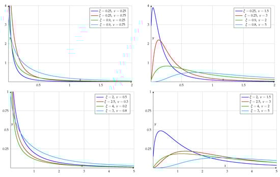
Figure 1. Graphs of the inverted Topp–Leone density for different values of $\xi$ and $\nu$.

By using the transformation $Z/\varphi =\sigma /X-1$ with the Jacobian $J(x\to z)={\displaystyle \frac{\sigma /\varphi }{{\left(1+z/\varphi \right)}^2}}$ in Equation (1), a different inverted Topp–Leone density can also be derived as

$$g(z;\nu ,\varphi )={\displaystyle \frac{2\nu }{\varphi }}\left({\displaystyle \frac{z}{\varphi }}\right){\left(1+{\displaystyle \frac{z}{\varphi }}\right)}^{-2\nu -1}{\left(1+{\displaystyle \frac{2z}{\varphi }}\right)}^{\nu -1},z>0,\nu >0.$$

(3)

Observe that Equation (3) can be obtained from Equation (2) by transforming $Y=1/Z$ with $\varphi =1/\xi$. This distribution, for $\varphi =1$, is defined and studied in Hassan, Elgarhy and Ragab [16]. For $\nu =1$, the inverted Topp–Leone density slides to a Pareto distribution given by the density

$${\displaystyle \frac{2}{\xi }}{\left(1+{\displaystyle \frac{y}{\xi }}\right)}^{-3},y>0.$$

By using Equation (2), the CDF of Y is derived as

$$\begin{array}{cc}\hfill F_Y(y;\nu ,\xi )& ={\displaystyle \frac{2\nu }{\xi }}{\int }_0^y{\left({\displaystyle \frac{w}{\xi }}\right)}^{\nu -1}{\left(1+{\displaystyle \frac{w}{\xi }}\right)}^{-2\nu -1}{\left(2+{\displaystyle \frac{w}{\xi }}\right)}^{\nu -1}\mathrm{d}w\hfill \\ \hfill & =2\nu {\int }_{1/(1+y/\xi )}^{1}t{(1-t^2)}^{\nu -1}\mathrm{d}t,\hfill \end{array}$$

(4)

where we have used the substitution $t=1/(1+w/\xi )$ with $\mathrm{d}w=-t^{-1}\mathrm{d}t$ and changed the limit of integration. The final result is obtained by substituting $1-t^2=u$ and evaluating the resulting expression, obtaining

$$\begin{array}{c}\hfill F_Y(y;\nu ,\xi )={(1-{\beta }^2)}^{\nu }={\left[1-{\left({\displaystyle \frac{1}{1+y/\xi }}\right)}^2\right]}^{\nu }={\left[{\displaystyle \frac{(2+y/\xi )y/\xi }{{(1+y/\xi )}^2}}\right]}^{\nu },\end{array}$$

(5)

where $\beta =1/(1+y/\xi )$.

By using Equations (2) and (5), the truncated version of the inverted Topp–Loene distribution can be defined by the density

$$\begin{array}{cc}\hfill f_{\mathrm{TITL}}(y;\nu ,\xi )& ={\displaystyle \frac{f_{\mathrm{ITL}}(y;\nu ,\xi )}{F_Y(B;\nu ,\xi )-F_Y(A;\nu ,\xi )}}\hfill \\ \hfill & ={\displaystyle \frac{2\nu }{\xi C}}{\left({\displaystyle \frac{y}{\xi }}\right)}^{\nu -1}{\left(1+{\displaystyle \frac{y}{\xi }}\right)}^{-2\nu -1}{\left(2+{\displaystyle \frac{y}{\xi }}\right)}^{\nu -1},0<A<y<B<\infty ,\hfill \end{array}$$

(6)

where

$$C=F_Y(B;\nu ,\xi )-F_Y(A;\nu ,\xi )={\left[{\displaystyle \frac{(2+B/\xi )B/\xi }{{(1+B/\xi )}^2}}\right]}^{\nu }-{\left[{\displaystyle \frac{(2+A/\xi )A/\xi }{{(1+A/\xi )}^2}}\right]}^{\nu }.$$

The quantile function $y_p=F_Y^{-1}\left(p\right)=Q_Y\left(p\right)$ is given by

$$Q_Y\left(p\right)=\xi \left[{(1-p^{1/\nu })}^{-1/2}-1\right],0<p<1.$$

The survival function (reliability function) and the hazard rate (failure rate) function of $Y\sim \mathrm{ITL}(\nu ;\xi )$ (Figure 2), by using the CDF of Y, can be obtained as

$$\begin{array}{cc}\hfill S_{\mathrm{ITL}}(y;\nu ,\xi )& =P(Y>y)={\overline{F}}_Y(y;\nu ,\xi )=1-F_Y(y;\nu ,\xi )\hfill \\ \hfill & =1-{(1-{\beta }^2)}^{\nu }=1-{\left[{\displaystyle \frac{(2+y/\xi )y/\xi }{{(1+y/\xi )}^2}}\right]}^{\nu }\hfill \end{array}$$

and

$$\begin{array}{c}\hfill {\lambda }_{\mathrm{ITL}}(y;\nu ,\xi )={\displaystyle \frac{f_{\mathrm{ITL}}(y;\nu ,\xi )}{1-F_Y(y;\nu ,\xi )}}={\displaystyle \frac{f_{\mathrm{ITL}}(y;\nu ,\xi )}{{\overline{F}}_Y(y;\nu ,\xi )}}={\displaystyle \frac{2\nu {\beta }^3{(1-{\beta }^2)}^{\nu -1}}{\xi [1-{\left(1-{\beta }^2\right)}^{\nu }]}}.\end{array}$$

(7)

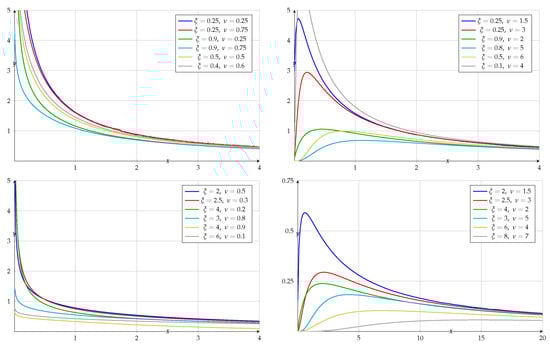
Figure 2. Graphs of the hazard rate function (Equation (7)) for different values of $\xi$ and $\nu$.

By using Equation (2), the Laplace transform of the density of Y, denoted by $L_Y\left(t\right)$, is derived as

$$\begin{array}{cc}\hfill L_Y\left(t\right)& ={\displaystyle \frac{2\nu }{\xi }}{\int }_0^{\infty }exp(-ty){\left({\displaystyle \frac{y}{\xi }}\right)}^{\nu -1}{\left(1+{\displaystyle \frac{y}{\xi }}\right)}^{-2\nu -1}{\left(2+{\displaystyle \frac{y}{\xi }}\right)}^{\nu -1}\mathrm{d}y\hfill \\ \hfill & =2\nu {\int }_0^{1}exp\left[-t\xi {\displaystyle \frac{1-u}{u}}\right]u{(1-u^2)}^{\nu -1}\mathrm{d}u,\hfill \end{array}$$

(8)

where we have used the substitution $u=1/(1+y/\xi )$. We will evaluate the above integral by using results on Laguerre polynomials.

The Laguerre polynomial of degree n is defined by the sum (for details see Nagar, Zarrazola and Sánchez [17]),

$$\begin{array}{c}\hfill L_n\left(x\right)=\sum _{k=0}^n{\displaystyle \frac{{(-1)}^k}{k!}}\left({\displaystyle \genfrac{}{}{0pt}{}{n}{k}}\right)x^k,\end{array}$$

where $\left({\displaystyle \genfrac{}{}{0pt}{}{n}{k}}\right)$ is the binomial coefficient. The first few Laguerre polynomials are

$$\begin{array}{cc}\hfill & L_0\left(x\right)=1,\hfill \\ \hfill & L_1\left(x\right)=-x+1,\hfill \\ \hfill & L_2\left(x\right)={\displaystyle \frac{1}{2}}(x^2-4x+2),\hfill \\ \hfill & L_3\left(x\right)={\displaystyle \frac{1}{6}}(-x^3+9x^2-18x+6).\hfill \end{array}$$

The first order derivative of the the Laguerre polynomial $L_n\left(x\right)$ is given by

$${\displaystyle \frac{\mathrm{d}}{\mathrm{d}x}}{L}_n\left(x\right)=-L_{n-1}^{\left(1\right)}\left(x\right)$$

where $L_n^{\left(\alpha \right)}\left(x\right)$ is the generalized Laguerre polynomial of degree n defined by the sum

$$L_n^{\left(\alpha \right)}\left(x\right)=\sum _{k=0}^n{\displaystyle \frac{{(-1)}^k}{k!}}\left({\displaystyle \genfrac{}{}{0pt}{}{n+\alpha }{n-k}}\right)x^k.$$

The generating function for the Laguerre polynomials is given by

$$\begin{array}{c}\hfill {\displaystyle \frac{exp[-xt/(1-t\left)\right]}{1-t}}=\sum _{n=0}^{\infty }{t}^n{L}_n\left(x\right),\left|t\right|<1.\end{array}$$

Replacing $exp\left[-t\xi {\displaystyle \frac{1-u}{u}}\right]$ by its series expansion involving Laguerre polynomials (Miller [18] Equations (3.4a) and (3.4b)), namely,

$$\begin{array}{c}\hfill exp\left[-t\xi {\displaystyle \frac{1-u}{u}}\right]=u\sum _{m=0}^{\infty }{L}_m\left(\xi t\right){(1-u)}^m,\left|u\right|<1,\end{array}$$

(9)

in Equation (8), we get

$$\begin{array}{cc}\hfill L_Y\left(t\right)& =2\nu \sum _{m=0}^{\infty }{L}_m\left(\xi t\right){\int }_0^1{u}^2{(1-u)}^m{(1-u^2)}^{\nu -1}\mathrm{d}u.\hfill \end{array}$$

(10)

By integrating the above expression, we get the Laplace transform of the density of Y.

Finally, we give the following theorems summarizing results given in Section 1 and this section.

Theorem 1. 

If $X\sim \mathrm{TL}(\nu ;\sigma )$ and $Y/\xi =X/(\sigma -X)$, $\xi >0$, then $Y\sim \mathrm{ITL}(\nu ;\xi )$. Further, if $Y\sim \mathrm{ITL}(\nu ;\xi )$ then $X=\sigma Y/\xi /(1+Y/\xi )\sim \mathrm{TL}(\nu ;\sigma )$.

Proof. 

Transforming $Y/\xi =X/(\sigma -X)$ with the Jacobian $J(x\to y)={\displaystyle \frac{\sigma /\xi }{{(1+y/\xi )}^2}}$ in Equation (1), we get the desired result. The second part is similar.    □

Theorem 2. 

Let $Y\sim \mathrm{ITL}(\nu ;\xi )$ and $U={\left(1+Y/\xi \right)}^{-1}$. Then, U follows a generalized Kumaraswamy distribution (Jones [19]) given by the density

$$2\nu u{(1-u^2)}^{\nu -1},0<u<1$$

and $U^2$ has a beta distribution with parameters 1 and ν.

Proof. 

Making the transformation $U={\left(1+Y/\xi \right)}^{-1}$ with the Jacobian $J(y\to u)=\xi u^{-2}$ in Equation (2), we get the density of U. Transforming $Z=U^2$ with the Jacobian $J(u\to z)=1/2\sqrt{z}$ in the density of U, the density of Z, denoted by $f_Z\left(z\right)$, is $f_Z\left(z\right)=\nu {(1-z)}^{\nu -1}$, $0<z<1$, which is a beta density with parameters 1 and $\nu$.    □

Theorem 3. 

Let $Y\sim \mathrm{ITL}(\nu ;\xi )$ and $U={\left[{\displaystyle \frac{(2+Y/\xi )Y/\xi }{{(1+Y/\xi )}^2}}\right]}^{\nu }$. Then, U follows a uniform distribution with support in $(0,1)$. Further, $-ln\left(U\right)$ and $-ln(1-U)$ follow standard exponential distribution.

Proof. 

Application of probability integral transformation (Bain and Engelhardt [20] p. 201) yields the desired result. The second part follows by applying the transformation $Z=-ln\left(U\right)$.    □

3. Expected Values

Using Theorem 2, it is easy to see that

$$\mathrm{E}\left[{\left(1+{\displaystyle \frac{Y}{\xi }}\right)}^{-2k}\right]={\displaystyle \frac{\mathrm{\Gamma }(k+1)\mathrm{\Gamma }(\nu +1)}{\mathrm{\Gamma }(\nu +k+1)}},k>-1.$$

For a non-negative integer r and an arbitrary $\delta$, the r-th moment of $Y^{1/\delta }$ is derived as

$$\begin{array}{cc}\hfill \mathrm{E}\left(Y^{r/\delta }\right)& ={\displaystyle \frac{2\nu }{{\xi }^{\nu }}}{\int }_0^{\infty }{y}^{\nu +r/\delta -1}{\left(1+{\displaystyle \frac{y}{\xi }}\right)}^{-2\nu -1}{\left(2+{\displaystyle \frac{y}{\xi }}\right)}^{\nu -1}\mathrm{d}y\hfill \\ \hfill & =2\nu {\xi }^{r/\delta }{\int }_0^1{u}^{\nu +r/\delta -1}{(1-u)}^{1-r/\delta }{(2-u)}^{\nu -1}\mathrm{d}u\hfill \\ \hfill & =2^{\nu }\nu {\xi }^{r/\delta }{\displaystyle \frac{\mathrm{\Gamma }(\nu +r/\delta )\mathrm{\Gamma }(2-r/\delta )}{\mathrm{\Gamma }(\nu +2)}}F\left(\nu +{\displaystyle \frac{r}{\delta }},1-\nu ;\nu +2;{\displaystyle \frac{1}{2}}\right),{\displaystyle \frac{r}{\delta }}<2,\hfill \end{array}$$

(11)

where we have used the substitution $y/\xi =u/(1-u)$ with $\mathrm{d}y=\xi {(1-u)}^{-2}\mathrm{d}u$ and the definition of the Gauss hypergeometric function (see (A1)). For $r=\delta$, using the substitution $1-u=t$ in Equation (11), one gets

$$\begin{array}{cc}\hfill \mathrm{E}\left(Y\right)& =2\nu \xi {\int }_0^1{(1-t^2)}^{\nu -1}\mathrm{d}t-2\xi \nu {\int }_0^{1}t{(1-t^2)}^{\nu -1}\mathrm{d}t\hfill \\ \hfill & =\xi \left[{\displaystyle \frac{\sqrt{\pi }\mathrm{\Gamma }(\nu +1)}{\mathrm{\Gamma }(\nu +1/2)}}-1\right].\hfill \end{array}$$

The above result can also be obtained by using (7.3.7.9) of Prudnikov, Brychkov and Marichev [21] p. 414.

Further, if $Y\sim \mathrm{ITL}(\nu ;\xi )$, then by using Theorem 3, it is straightforward to show that

$$\begin{array}{c}\hfill \mathrm{E}{\left[\left({\displaystyle \frac{Y}{\xi }}\right)\left(2+{\displaystyle \frac{Y}{\xi }}\right){\left(1+{\displaystyle \frac{Y}{\xi }}\right)}^{-2}\right]}^k={\displaystyle \frac{\nu }{\nu +k}}.\end{array}$$

Theorem 4. 

If $Y\sim \mathrm{ITL}(\nu ;\xi )$, then

$$\begin{array}{c}\hfill \mathrm{E}\left[{\left({\displaystyle \frac{Y}{\xi }}\right)}^k{\left(2+{\displaystyle \frac{Y}{\xi }}\right)}^{-\ell }\right]=\nu \sum _{j=0}^{k+\ell }\left({\displaystyle \genfrac{}{}{0pt}{}{k+\ell }{j}}\right){(-1)}^j{\displaystyle \frac{\mathrm{\Gamma }(1+(\ell -k+j)/2)\mathrm{\Gamma }(\nu -\ell )}{\mathrm{\Gamma }[\nu +1+(j-\ell -k)/2]}},\end{array}$$

where $\nu >max\{\ell ,(\ell +k)/2-1\}$ and $1+(\ell -k)/2>0$.

Proof. 

By definition

$$\begin{array}{cc}\hfill \mathrm{E}\left[{\left({\displaystyle \frac{Y}{\xi }}\right)}^k{\left(2+{\displaystyle \frac{Y}{\xi }}\right)}^{-\ell }\right]& ={\displaystyle \frac{2\nu }{{\xi }^{\nu +k}}}{\int }_0^{\infty }{y}^{\nu +k-1}{\left(1+{\displaystyle \frac{y}{\xi }}\right)}^{-2\nu -1}{\left(2+{\displaystyle \frac{y}{\xi }}\right)}^{\nu -\ell -1}\mathrm{d}y\hfill \\ \hfill & =2\nu {\int }_0^{\infty }{(1-t)}^{\ell +k}{t}^{\ell -k+1}{(1-t^2)}^{\nu -\ell -1}\mathrm{d}t,\hfill \end{array}$$

where we have used the substitution $y/\xi =(1-t)/t$. Now, expanding ${\left(1-t\right)}^{k+\ell }$ using binomial theorem and substituting $t^2=z$, we obtain

$$\begin{array}{c}\hfill \mathrm{E}\left[{\left({\displaystyle \frac{Y}{\xi }}\right)}^k{\left(2+{\displaystyle \frac{Y}{\xi }}\right)}^{-\ell }\right]=\nu \sum _{j=0}^{k+\ell }\left({\displaystyle \genfrac{}{}{0pt}{}{k+\ell }{j}}\right){(-1)}^j{\int }_0^{\infty }{z}^{(\ell +j-k)/2}{\left(1-z\right)}^{\nu -\ell -1}\mathrm{d}z.\end{array}$$

Finally, integrating z by using the definition of beta function, the desired result in obtained.    □

Corollary 1. 

If $Y\sim \mathrm{ITL}(\nu ;\xi )$, then for $\nu -k>0$,

$$\begin{array}{c}\hfill \mathrm{E}\left[{\left({\displaystyle \frac{Y}{\xi }}\right)}^k{\left(2+{\displaystyle \frac{Y}{\xi }}\right)}^{-k}\right]=\nu \sum _{j=0}^{2k}\left({\displaystyle \genfrac{}{}{0pt}{}{2k}{j}}\right){(-1)}^j{\displaystyle \frac{\mathrm{\Gamma }(1+j/2)\mathrm{\Gamma }(\nu -k)}{\mathrm{\Gamma }(\nu -k+1+j/2)}}.\end{array}$$

Proof. 

Substituting $\ell =k$ in the above theorem, we easily get the result.    □

Substituting $k=1$ and $k=2$ in the above corollary and simplifying, one gets

$$\begin{array}{c}\hfill \mathrm{E}\left[{\displaystyle \frac{Y/\xi }{2+Y/\xi }}\right]={\displaystyle \frac{\nu +1}{\nu -1}}-{\displaystyle \frac{\sqrt{\pi }\nu \mathrm{\Gamma }(\nu -1)}{\mathrm{\Gamma }\left(\nu +1/2\right)}},\nu >1,\end{array}$$

(12)

and

$$\begin{array}{c}\hfill \mathrm{E}{\left[{\displaystyle \frac{Y/\xi }{2+Y/\xi }}\right]}^2={\displaystyle \frac{{\nu }^2+5\nu +2}{(\nu -1)(\nu -2)}}-{\displaystyle \frac{2\sqrt{\pi }(\nu +1)\nu \mathrm{\Gamma }(\nu -2)}{\mathrm{\Gamma }\left(\nu +1/2\right)}},\nu >2.\end{array}$$

(13)

Also, substituting $(k,\ell )=(1,2)$ in the above theorem and simplifying the resulting expression, we get

$$\begin{array}{c}\hfill \mathrm{E}\left[\left({\displaystyle \frac{Y}{\xi }}\right){\left(2+{\displaystyle \frac{Y}{\xi }}\right)}^{-2}\right]={\displaystyle \frac{\sqrt{\pi }(\nu +4)\nu \mathrm{\Gamma }(\nu -2)}{2\mathrm{\Gamma }(\nu +1/2)}}-{\displaystyle \frac{3\nu +2}{(\nu -1)(\nu -2)}},\nu >2.\end{array}$$

Similarly, one can easily derive the following theorem:

Theorem 5. 

If $Y\sim \mathrm{ITL}(\nu ;\xi )$, then

$$\begin{array}{c}\hfill \mathrm{E}\left[{\left({\displaystyle \frac{Y}{\xi }}\right)}^k{\left(1+{\displaystyle \frac{Y}{\xi }}\right)}^{-k}\right]=\nu \sum _{j=0}^k\left({\displaystyle \genfrac{}{}{0pt}{}{k}{j}}\right){(-1)}^j{\displaystyle \frac{\mathrm{\Gamma }(1+j/2)\mathrm{\Gamma }\left(\nu \right)}{\mathrm{\Gamma }(\nu +1+j/2)}}.\end{array}$$

Proof. 

By using Equation (2), we have

$$\begin{array}{cc}\hfill \mathrm{E}\left[{\left({\displaystyle \frac{Y}{\xi }}\right)}^k{\left(1+{\displaystyle \frac{Y}{\xi }}\right)}^{-k}\right]& ={\displaystyle \frac{2\nu }{\xi }}{\int }_0^{\infty }{\left({\displaystyle \frac{y}{\xi }}\right)}^{\nu +k-1}{\left(1+{\displaystyle \frac{y}{\xi }}\right)}^{-2\nu -k-1}{\left(2+{\displaystyle \frac{y}{\xi }}\right)}^{\nu -1}\mathrm{d}y\hfill \\ \hfill & =2\nu {\int }_0^1{(1-t)}^{k}t{(1-t^2)}^{\nu -1}\mathrm{d}t,\hfill \end{array}$$

where we have used the substitution $y/\xi =(1-t)/t$. Now, expanding ${\left(1-t\right)}^k$ using binomial theorem and substituting $t^2=z$, we obtain

$$\begin{array}{cc}\hfill \mathrm{E}\left[{\left({\displaystyle \frac{Y}{\xi }}\right)}^k{\left(1+{\displaystyle \frac{Y}{\xi }}\right)}^{-k}\right]& =\nu \sum _{j=0}^k\left({\displaystyle \genfrac{}{}{0pt}{}{k}{j}}\right){(-1)}^j{\int }_0^1{z}^{j/2}{(1-z)}^{\nu -1}\mathrm{d}z.\hfill \end{array}$$

Finally, the desired result is obtained by using the definition of the beta function.    □

By substituting $k=1$ and $k=2$ in the above theorem and simplifying, one gets

$$\begin{array}{c}\hfill \mathrm{E}\left[{\displaystyle \frac{Y/\xi }{1+Y/\xi }}\right]=1-{\displaystyle \frac{\sqrt{\pi }\mathrm{\Gamma }(\nu +1)}{2\mathrm{\Gamma }(\nu +3/2)}}\end{array}$$

(14)

and

$$\begin{array}{c}\hfill \mathrm{E}{\left[{\displaystyle \frac{Y/\xi }{1+Y/\xi }}\right]}^2={\displaystyle \frac{\nu +2}{\nu +1}}-{\displaystyle \frac{\sqrt{\pi }\mathrm{\Gamma }(\nu +1)}{\mathrm{\Gamma }(\nu +3/2)}}.\end{array}$$

(15)

Observe that ${\displaystyle \frac{Y/\xi }{1+Y/\xi }}\sim TL({\nu }_1+{\nu }_2)$ and therefore the above results can be obtained from the moments of T-L distribution, see Nadrajah [3], Nagar, Zarrazola and Echeverri-Valencia [22].

Several interesting cases of expected values of functions of the ITL variable can be obtained by using results derived in this section. Using Equations (12)–(15), one gets

$$\begin{array}{cc}\hfill 2\mathrm{E}\left[{\displaystyle \frac{Y/\xi }{1+Y/\xi }}\right]-\mathrm{E}\left[{\displaystyle \frac{Y/\xi }{2+Y/\xi }}\right]& =2-{\displaystyle \frac{\sqrt{\pi }\mathrm{\Gamma }(\nu +1)}{\mathrm{\Gamma }(\nu +3/2)}}-{\displaystyle \frac{\nu +1}{\nu -1}}+{\displaystyle \frac{\sqrt{\pi }\nu \mathrm{\Gamma }(\nu -1)}{\mathrm{\Gamma }\left(\nu +1/2\right)}}\hfill \\ \hfill & ={\displaystyle \frac{3\sqrt{\pi }\mathrm{\Gamma }(\nu +1)}{2(\nu -1)\mathrm{\Gamma }(\nu +3/2)}}+{\displaystyle \frac{\nu -3}{\nu -1}},\nu >1,\hfill \end{array}$$

(16)

$$\begin{array}{cc}\hfill \mathrm{E}{\left[{\displaystyle \frac{Y/\xi }{1+Y/\xi }}\right]}^2-2\mathrm{E}\left[{\displaystyle \frac{Y/\xi }{1+Y/\xi }}\right]& ={\displaystyle \frac{\nu +2}{\nu +1}}-{\displaystyle \frac{\sqrt{\pi }\mathrm{\Gamma }(\nu +1)}{\mathrm{\Gamma }(\nu +3/2)}}-2+{\displaystyle \frac{\sqrt{\pi }\mathrm{\Gamma }(\nu +1)}{\mathrm{\Gamma }(\nu +3/2)}}\hfill \\ \hfill & =-{\displaystyle \frac{\nu }{\nu +1}},\hfill \end{array}$$

(17)

$$\begin{array}{cc}\hfill \mathrm{E}{\left[{\displaystyle \frac{Y/\xi }{2+Y/\xi }}\right]}^2-2\mathrm{E}\left[{\displaystyle \frac{Y/\xi }{2+Y/\xi }}\right]& ={\displaystyle \frac{{\nu }^2+5\nu +2}{(\nu -1)(\nu -2)}}-{\displaystyle \frac{2\sqrt{\pi }(\nu +1)\nu \mathrm{\Gamma }(\nu -2)}{\mathrm{\Gamma }\left(\nu +1/2\right)}}\hfill \\ \hfill & -2{\displaystyle \frac{\nu +1}{\nu -1}}+2{\displaystyle \frac{\sqrt{\pi }\nu \mathrm{\Gamma }(\nu -1)}{\mathrm{\Gamma }\left(\nu +1/2\right)}}\hfill \\ \hfill & ={\displaystyle \frac{-{\nu }^2+7\nu +6}{(\nu -1)(\nu -2)}}-{\displaystyle \frac{6\sqrt{\pi }\nu \mathrm{\Gamma }(\nu -2)}{\mathrm{\Gamma }\left(\nu +1/2\right)}},\nu >2.\hfill \end{array}$$

(18)

4. Stress-Strength Reliability Model

Inferences about $R=P[Y<X]$, where X and Y are two independent random variables, are very common in reliability, statistical tolerance and biometry (Ali and Woo [23], Kotz, Lumelskii and Pensky [24]).

Let Y represent the random variable of a stress that a device will be subjected to in service, and let X represent the strength that varies from item to item in the population of devices. Then, the reliability, which is the probability that a randomly selected device functions successfully, denoted by R, is equal to $P(Y<X)$.

Let Y and X be the stress and the strength random variables, independent of each other, $Y\sim \mathrm{ITL}(\nu ;\xi )$ and $X\sim \mathrm{ITL}(\mu ;\xi )$; then,

$$\begin{array}{cc}\hfill R=P(Y<X)& ={\int }_0^{\infty }{f}_{\mathrm{ITL}}(x;\mu ,\xi )F_Y(x;\nu ,\xi )\mathrm{d}x\hfill \\ \hfill & ={\displaystyle \frac{2\mu }{\xi }}{\int }_0^{\infty }{\left({\displaystyle \frac{x}{\xi }}\right)}^{\mu -1}{\left(1+{\displaystyle \frac{x}{\xi }}\right)}^{-2\mu -1}{\left(2+{\displaystyle \frac{x}{\xi }}\right)}^{\mu -1}{\left[{\displaystyle \frac{(2+x/\xi )x/\xi }{{(1+x/\xi )}^2}}\right]}^{\nu }\mathrm{d}x\hfill \\ \hfill & ={\displaystyle \frac{2\mu }{\xi }}{\int }_0^{\infty }{\left({\displaystyle \frac{x}{\xi }}\right)}^{\mu +\nu -1}{\left(1+{\displaystyle \frac{x}{\xi }}\right)}^{-2(\mu +\nu )-1}{\left(2+{\displaystyle \frac{x}{\xi }}\right)}^{\mu +\nu -1}\mathrm{d}x\hfill \\ \hfill & ={\displaystyle \frac{2\mu }{\xi }}{\displaystyle \frac{\xi }{2(\mu +\nu )}}={\displaystyle \frac{\mu }{\mu +\nu }}.\hfill \end{array}$$

5. Order Statistics

This section gives the pdf of the i-th order statistic from a sample of size n drawn from an inverted Topp–Leone population. The pdf of the i-th order statistic, when a sample of size n is available from a continuous distribution with pdf $f_X\left(x\right)$, where $f_X\left(x\right)>0$ for $a<x<b$, and CDF $F_X\left(x\right)$, is given by (Bain and Engelhardt [20] p. 217),

$$g_i\left(y\right)={\displaystyle \frac{n!}{(i-1)!(n-i)!}}{\left[F_X\left(y\right)\right]}^{i-1}{[1-F_X\left(y\right)]}^{n-i}{f}_x\left(y\right),a<x<b.$$

If $Y_1<Y_{\left(2\right)}<\dots <Y_{\left(n\right)}$ are order statistics from an inverted Topp–Leone distribution, then the density of i-th order statistic $Y_{\left(i\right)}$, denoted by $g_i\left(y\right)$, $1\le i\le n$, is given by

$$\begin{array}{cc}\hfill g_i\left(y\right)& ={\displaystyle \frac{n!}{i!(n-i)!}}{\displaystyle \frac{2i\nu }{\xi }}{\left({\displaystyle \frac{y}{\xi }}\right)}^{i\nu -1}{\left(1+{\displaystyle \frac{y}{\xi }}\right)}^{-2i\nu -1}{\left(2+{\displaystyle \frac{y}{\xi }}\right)}^{i\nu -1}{\left[1-{\left[{\displaystyle \frac{(2+y/\xi )y/\xi }{{(1+y/\xi )}^2}}\right]}^{\nu }\right]}^{n-i},y>0.\hfill \end{array}$$

where we have used Equations (2) and (5) for the pdf and CDF. Finally, re-writing the above expression, we get

$$\begin{array}{cc}\hfill g_i\left(y\right)& ={\displaystyle \frac{n!}{i!(n-i)!}}{f}_{\mathrm{ITL}}(y;i\nu ,\xi ){\left[1-{\left[{\displaystyle \frac{(2+y/\xi )y/\xi }{{(1+y/\xi )}^2}}\right]}^{\nu }\right]}^{n-i},y>0.\hfill \end{array}$$

It is interesting to note that $Y_{\left(n\right)}\sim \mathrm{ITL}(n\nu ;\xi )$ and the density of $Y_1$ is given by

$$\begin{array}{c}\hfill g_1\left(y\right)=n{\displaystyle \frac{2\nu }{\xi }}{\left({\displaystyle \frac{y}{\xi }}\right)}^{\nu -1}{\left(1+{\displaystyle \frac{y}{\xi }}\right)}^{-2\nu -1}{\left(2+{\displaystyle \frac{y}{\xi }}\right)}^{\nu -1}{\left[1-{\left[{\displaystyle \frac{(2+y/\xi )y/\xi }{{(1+y/\xi )}^2}}\right]}^{\nu }\right]}^{n-1},y>0.\end{array}$$

The density of sample media when n is odd, say $n=2m+1$, can also be obtained by substituting $i=m=(n-1)/2$ in the density of $Y_{\left(i\right)}$.

6. Entropy

An entropy of a random variable is a measure of variation of uncertainty. In this section we will derive two entropies know as Shannon and Rényi entropies for the inverted Topp–Leone distribution.

Denote by $H_{SH}\left(f\right)$ the well-known Shannon entropy introduced in Shannon [25]. It is define by

$$\begin{array}{c}\hfill H_{SH}\left(f\right)=-\int f\left(x\right)logf\left(x\right)\mathrm{d}x.\end{array}$$

(19)

One of the main extensions of the Shannon entropy was defined by Rényi [26]. This generalized entropy measure is given by

$$\begin{array}{c}\hfill H_R(\eta ,f)={\displaystyle \frac{logG\left(\eta \right)}{1-\eta }}(\mathrm{for}\eta >0\mathrm{and}\eta \ne 1),\end{array}$$

(20)

where

$$\begin{array}{c}\hfill G\left(\eta \right)=\int f^{\eta }\left(x\right)dx.\end{array}$$

The additional parameter $\eta$ is used to describe complex behavior in probability models and the associated process under study. Rényi entropy is monotonically decreasing in $\eta$, while Shannon entropy (Equation (19)) is obtained from Equation (20) for $\eta \uparrow 1$. For details see Nadarajah and Zografos [27], Zografos and Nadarajah [28] and Zografos [29].

Theorem 6. 

For the inverted Topp–Leone distribution defined by Equation (2), the Rényi and the Shannon entropies are given by

$$\begin{array}{cc}\hfill H_R(\eta ,f)& ={\displaystyle \frac{1}{1-\eta }}[\eta ln\nu +(\eta -1)ln\left({\displaystyle \frac{2}{\xi }}\right)+ln\mathrm{\Gamma }\left[\eta (\nu -1)+1\right]+ln\mathrm{\Gamma }\left({\displaystyle \frac{3\eta -1}{2}}\right)\hfill \\ \hfill & -ln\mathrm{\Gamma }\left[\eta \left(\nu +{\displaystyle \frac{1}{2}}\right)+{\displaystyle \frac{1}{2}}\right]],\eta >{\displaystyle \frac{1}{3}}\hfill \end{array}$$

and

$$\begin{array}{cc}\hfill H_{SH}\left(f\right)& =-ln\left({\displaystyle \frac{2\nu }{\xi }}\right)-(\nu -1)\psi \left(\nu \right)-{\displaystyle \frac{3}{2}}\psi \left({\displaystyle \frac{1}{2}}\right)+\left(\nu +{\displaystyle \frac{1}{2}}\right)\psi (\nu +1)\hfill \\ \hfill & =-ln\left({\displaystyle \frac{2\nu }{\xi }}\right)+(\nu -1)[\psi (\nu +1)-\psi \left(\nu \right)]+{\displaystyle \frac{3}{2}}[\psi (\nu +1)-\psi \left({\displaystyle \frac{1}{2}}\right)]\hfill \\ \hfill & =-ln\left({\displaystyle \frac{2\nu }{\xi }}\right)+{\displaystyle \frac{\nu -1}{\nu }}+{\displaystyle \frac{3}{2}}\left[\psi (\nu +1)-\psi \left({\displaystyle \frac{1}{2}}\right)\right],\hfill \end{array}$$

respectively, where $\psi \left(\alpha \right)={\mathrm{\Gamma }}^{\prime }\left(\alpha \right)/\mathrm{\Gamma }\left(\alpha \right)$ is the digamma function.

Proof. 

For $\eta >0$ and $\eta \ne 1$, using the density of Y given by Equation (2), we have

$$\begin{array}{cc}\hfill G\left(\eta \right)& ={\left({\displaystyle \frac{2\nu }{\xi }}\right)}^{\eta }{\int }_0^{\infty }{\left({\displaystyle \frac{w}{\xi }}\right)}^{\eta (\nu -1)}{\left(1+{\displaystyle \frac{w}{\xi }}\right)}^{-\eta (2\nu +1)}{\left(2+{\displaystyle \frac{w}{\xi }}\right)}^{\eta (\nu -1)}\mathrm{d}w\hfill \\ \hfill & ={\left({\displaystyle \frac{2\nu }{\xi }}\right)}^{\eta }\xi {\int }_0^1{t}^{3\eta -2}{(1-t^2)}^{\eta (\nu -1)}\mathrm{d}t,\hfill \end{array}$$

(21)

where the last line has been obtained by substituting $t=1/(1+w/\xi )$. The final result is obtained by substituting $1-t^2=u$ and evaluating the resulting expression by using beta integrals,

$$\begin{array}{c}\hfill G\left(\eta \right)={\nu }^{\eta }{\left({\displaystyle \frac{2}{\xi }}\right)}^{\eta -1}{\displaystyle \frac{\mathrm{\Gamma }\left[\eta \right(\nu -1)+1]\mathrm{\Gamma }\left[\right(3\eta -1)/2]}{\mathrm{\Gamma }\left[\eta \right(\nu +1/2)+1/2]}},\eta >1/3.\end{array}$$

(22)

Now, taking logarithm of $G\left(\eta \right)$ and using Equation (20) we get $H_R(\eta ,f)$. The Shannon entropy is obtained from $H_R(\eta ,f)$ by taking $\eta \uparrow 1$ and using L’Hopital’s rule.    □

7. Estimation and Information Matrix

Let $Y_1,\dots ,Y_n$ be a random sample from the inverted Topp–Leone distribution defined by Equation (2). The log-likelihood function, denoted by $l(\nu ,\xi )$, is given by

$$\begin{array}{cc}\hfill l(\nu ,\xi )& =n\left[ln2+ln\nu -\nu ln\xi \right]+(\nu -1)\sum _{i=1}^{n}ln{y}_i-(2\nu +1)\sum _{i=1}^{n}ln\left(1+{\displaystyle \frac{y_i}{\xi }}\right)\hfill \\ \hfill & +(\nu -1)\sum _{i=1}^{n}ln\left(2+{\displaystyle \frac{y_i}{\xi }}\right),\hfill \end{array}$$

Now, differentiating $l(\nu ,\xi )$ wrt $\nu$, we get

$$\begin{array}{cc}\hfill {\displaystyle \frac{\partial l(\nu ,\xi )}{\partial \nu }}& ={\displaystyle \frac{n}{\nu }}-nln\xi +\sum _{i=1}^{n}ln{y}_i-2\sum _{i=1}^{n}ln\left(1+{\displaystyle \frac{y_i}{\xi }}\right)+\sum _{i=1}^{n}ln\left(2+{\displaystyle \frac{y_i}{\xi }}\right),\hfill \end{array}$$

(23)

Further, differentiating wrt $\xi$, one gets

$$\begin{array}{cc}\hfill {\displaystyle \frac{\partial l(\nu ,\xi )}{\partial \xi }}& =-{\displaystyle \frac{n\nu }{\xi }}+{\displaystyle \frac{2\nu +1}{\xi }}\sum _{i=1}^n{\displaystyle \frac{y_i/\xi }{1+y_i/\xi }}-{\displaystyle \frac{\nu -1}{\xi }}\sum _{i=1}^n{\displaystyle \frac{y_i/\xi }{2+y_i/\xi }}.\hfill \end{array}$$

(24)

Thus, by solving numerically Equations (23) and (24), the MLEs of the $\nu$ and $\xi$ can be obtained. As the MLEs are not in a closed form, a Python (latest v3.14) code is developed to get the estimates. However, if the parameter $\xi$ has a fixed value, say $\xi ={\xi }_0$, then the MLE of $\nu$ can be given by

$$\widehat{\nu }=-n{\left[\sum _{i=1}^{n}ln{\displaystyle \frac{(2+Y_i/{\xi }_0)Y_i/{\xi }_0}{{(1+Y_i/{\xi }_0)}^2}}\right]}^{-1}.$$

Note that we can write $-\nu {\sum }_{i=1}^{n}ln{\displaystyle \frac{(2+Y_i/{\xi }_0)Y_i/{\xi }_0}{{(1+Y_i/{\xi }_0)}^2}}=-{\sum }_{i=1}^{n}ln{U}_i$, where $U_1,\dots ,U_n$ are independent random variables. Also, from Theorem 3, $-ln{U}_i$ follows an exponential distribution with mean 1, and therefore $-\nu {\sum }_{i=1}^{n}ln{\displaystyle \frac{(2+Y_i/{\xi }_0)Y_i/{\xi }_0}{{(1+Y_i/{\xi }_0)}^2}}$ is distributed as gamma with shape parameter 1 and scale parameter n. Now, using results on gamma distribution, we get

$$\mathrm{E}\left({\widehat{\nu }}^r\right)={\left(n\nu \right)}^r{\displaystyle \frac{\mathrm{\Gamma }(n-r)}{\mathrm{\Gamma }\left(n\right)}},n>r$$

from which the mean, the variance and the MSE of $\widehat{\nu }$ are calculated as $\mathrm{E}\left(\widehat{\nu }\right)=n\nu /(n-1)$, $\mathrm{Var}\left(\widehat{\nu }\right)=n^2{\nu }^2/{(n-1)}^2(n-2)$ and $\mathrm{MSE}\left(\widehat{\nu }\right)=(n+2){\nu }^2/(n-1)(n-2)$, respectively. Further, the unbiased estimator $\widehat{.3ex\phantom{\nu }\widehat{\nu }}=(n-1)\widehat{\nu }/n$ has variance $\mathrm{Var}\left(\widehat{.3ex\phantom{\nu }\widehat{\nu }}\right)={\nu }^2/(n-2)$ bigger than the Rao-Cramér lower bound, which is ${\nu }^2/n$. For a fixed value of $\nu$, say ${\nu }_0$, the statistic $-2{\nu }_0{\sum }_{i=1}^{n}ln{\displaystyle \frac{(2+Y_i/{\xi }_0)Y_i/{\xi }_0}{{(1+Y_i/{\xi }_0)}^2}}$ has a chi-square distribution with $2n$ degrees of freedom and could be used to test the hypothesis $H:\xi ={\xi }_0$.

Further differentiating Equations (23) and (24) with respect to $\nu$ and $\xi$, respectively, the second-order derivatives are derived as

$$\begin{array}{cc}\hfill {\displaystyle \frac{{\partial }^{2}l(\nu ,\xi )}{\partial {\nu }^2}}& =-{\displaystyle \frac{n}{{\nu }^2}},\hfill \end{array}$$

(25)

$$\begin{array}{cc}\hfill {\displaystyle \frac{{\partial }^{2}l(\nu ,\xi )}{\partial \xi \partial \nu }}& =-{\displaystyle \frac{n}{\xi }}+{\displaystyle \frac{2}{\xi }}\sum _{i=1}^n{\displaystyle \frac{y_i/\xi }{\left(1+y_i/\xi \right)}}-{\displaystyle \frac{1}{\xi }}\sum _{i=1}^n{\displaystyle \frac{y_i/\xi }{\left(2+y_i/\xi \right)}}.\hfill \end{array}$$

(26)

and

$$\begin{array}{cc}\hfill {\displaystyle \frac{{\partial }^{2}l(\nu ,\xi )}{\partial {\xi }^2}}& ={\displaystyle \frac{n\nu }{{\xi }^2}}+{\displaystyle \frac{2\nu +1}{{\xi }^2}}\sum _{i=1}^n\left[{\displaystyle \frac{{(y_i/\xi )}^2}{{\left(1+y_i/\xi \right)}^2}}-{\displaystyle \frac{2y_i/\xi }{\left(1+y_i/\xi \right)}}\right]\hfill \\ \hfill & -{\displaystyle \frac{\nu -1}{{\xi }^2}}\sum _{i=1}^n\left[{\displaystyle \frac{{(y_i/\xi )}^2}{{\left(2+y_i/\xi \right)}^2}}-{\displaystyle \frac{2(y_i/\xi )}{\left(2+y_i/\xi \right)}}\right].\hfill \end{array}$$

(27)

Note that the expected value of a constant is the constant itself and therefore

$$\begin{array}{c}\hfill \mathrm{E}\left[{\displaystyle \frac{{\partial }^{2}l(\nu ,\xi )}{\partial {\nu }^2}}\right]=-{\displaystyle \frac{n}{{\nu }^2}}.\end{array}$$

(28)

Further, since $Y_1,\dots ,Y_n$ are identically distributed, $Y_i\sim \mathrm{ITL}(\nu ;\xi )$, $i=1,\dots ,n$, from Equations (16)–(18), we have

$$\begin{array}{cc}\hfill \mathrm{E}\left[{\displaystyle \frac{{\partial }^{2}l(\nu ,\xi )}{\partial \xi \partial \nu }}\right]& =-{\displaystyle \frac{n}{\xi }}+{\displaystyle \frac{2}{\xi }}\sum _{i=1}^n\mathrm{E}\left[{\displaystyle \frac{Y_i/\xi }{\left(1+Y_i/\xi \right)}}\right]-{\displaystyle \frac{1}{\xi }}\sum _{i=1}^n\mathrm{E}\left[{\displaystyle \frac{Y_i/\xi }{\left(2+Y_i/\xi \right)}}\right]\hfill \\ \hfill & =-{\displaystyle \frac{n}{\xi }}+{\displaystyle \frac{2n}{\xi }}\mathrm{E}\left[{\displaystyle \frac{Y/\xi }{\left(1+Y/\xi \right)}}\right]-{\displaystyle \frac{n}{\xi }}\mathrm{E}\left[{\displaystyle \frac{Y/\xi }{\left(2+Y/\xi \right)}}\right]\hfill \\ \hfill & ={\displaystyle \frac{n}{\xi }}\left[{\displaystyle \frac{3\sqrt{\pi }\mathrm{\Gamma }(\nu +1)}{2(\nu -1)\mathrm{\Gamma }(\nu +3/2)}}-{\displaystyle \frac{2}{\nu -1}}\right],\nu >1,\hfill \end{array}$$

and

$$\begin{array}{cc}\hfill \mathrm{E}\left[{\displaystyle \frac{{\partial }^{2}l(\nu ,\xi )}{\partial {\xi }^2}}\right]& ={\displaystyle \frac{n\nu }{{\xi }^2}}+{\displaystyle \frac{2\nu +1}{{\xi }^2}}\sum _{i=1}^n\mathrm{E}\left[{\displaystyle \frac{{(Y_i/\xi )}^2}{{\left(1+Y_i/\xi \right)}^2}}-{\displaystyle \frac{2Y_i/\xi }{\left(1+Y_i/\xi \right)}}\right]\hfill \\ \hfill & -{\displaystyle \frac{\nu -1}{{\xi }^2}}\sum _{i=1}^n\mathrm{E}\left[{\displaystyle \frac{{(Y_i/\xi )}^2}{{\left(2+Y_i/\xi \right)}^2}}-{\displaystyle \frac{2(Y_i/\xi )}{\left(2+Y_i/\xi \right)}}\right]\hfill \\ \hfill & ={\displaystyle \frac{n\nu }{{\xi }^2}}+{\displaystyle \frac{n(2\nu +1)}{{\xi }^2}}\mathrm{E}\left[{\displaystyle \frac{{(Y/\xi )}^2}{{\left(1+Y/\xi \right)}^2}}-{\displaystyle \frac{2Y/\xi }{\left(1+Y/\xi \right)}}\right]\hfill \\ \hfill & -{\displaystyle \frac{n(\nu -1)}{{\xi }^2}}\mathrm{E}\left[{\displaystyle \frac{{(Y/\xi )}^2}{{\left(2+Y/\xi \right)}^2}}-{\displaystyle \frac{2(Y/\xi )}{\left(2+Y/\xi \right)}}\right]\hfill \\ \hfill & ={\displaystyle \frac{n}{{\xi }^2}}\left[{\displaystyle \frac{6\sqrt{\pi }\mathrm{\Gamma }(\nu +1)}{(\nu -2)\mathrm{\Gamma }\left(\nu +1/2\right)}}-{\displaystyle \frac{4{\nu }^2+13\nu +6}{(\nu -2)(\nu +1)}}\right],\nu >2,.\hfill \end{array}$$

For a given observation y, the Fisher information matrix for the inverted Topp–Leone distribution given by Equation (2) is defined as

$$\left(\begin{array}{cc}{\displaystyle \frac{1}{{\nu }^2}}& -{\displaystyle \frac{2}{\xi (\nu -1)}}\left[1-{\displaystyle \frac{3\sqrt{\pi }\mathrm{\Gamma }(\nu +1)}{4\mathrm{\Gamma }(\nu +3/2)}}\right]\\ -{\displaystyle \frac{2}{\xi (\nu -1)}}\left[1-{\displaystyle \frac{3\sqrt{\pi }\mathrm{\Gamma }(\nu +1)}{4\mathrm{\Gamma }(\nu +3/2)}}\right]& -{\displaystyle \frac{1}{{\xi }^2(\nu -2)}}\left[{\displaystyle \frac{6\sqrt{\pi }\mathrm{\Gamma }(\nu +1)}{\mathrm{\Gamma }\left(\nu +1/2\right)}}-{\displaystyle \frac{4{\nu }^2+13\nu +6}{\nu +1}}\right]\end{array}\right).$$

8. Partial Ordering

A random variable X with distribution function $F_X$ can be said to be greater than another random variable Y with distribution function $F_Y$ in a number of ways. There are several different concepts of partial ordering between random variables, such as likelihood ratio ordering, hazard rate ordering, reverse hazard rate ordering, and stochastic ordering. A random variable X is stochastically greater than a random variable Y, written as $X\stackrel{\mathrm{st}}{\ge }Y$, if $P(X>t)\ge P(Y>t)$ (equivalently ${\overline{F}}_X\left(t\right)\ge {\overline{F}}_Y\left(t\right)$) for all t. Here, in this section, we denote by $f_X\left(t\right)$ and ${\overline{F}}_X\left(t\right)=1-F_X\left(t\right)$ the density function and the survival function, respectively, of X. A random variable X is considered to be larger than a random variable Y in the hazard rate ordering (denoted by $X\stackrel{\mathrm{hr}}{\ge }Y$), if

$${\lambda }_X\left(t\right)={\displaystyle \frac{f_X\left(t\right)}{{\overline{F}}_X\left(t\right)}}\le {\lambda }_Y\left(t\right)={\displaystyle \frac{f_Y\left(t\right)}{{\overline{F}}_Y\left(t\right)}}$$

for all $t\ge 0$. The condition ${\lambda }_X\left(t\right)\le {\lambda }_Y\left(t\right)$ is equivalent to the condition that the function ${\overline{F}}_X\left(t\right)/{\overline{F}}_Y\left(t\right)$ is non-decreasing in t. The random variable Y is said to be smaller than the random variable X in the reverse hazard rate order (written as $X\stackrel{\mathrm{rhr}}{\ge }Y$) if $F_X\left(t\right)/F_Y\left(t\right)$ is non-decreasing in t. We state that X is larger than a random variable Y according to the likelihood ratio ordering (written as $X\stackrel{\mathrm{lr}}{\ge }Y$) if $f_X\left(t\right)/f_Y\left(t\right)$ is non-decreasing function of t.

It is well known that $X\stackrel{\mathrm{lr}}{\ge }Y\Rightarrow X\stackrel{\mathrm{hr}}{\ge }Y\Rightarrow X\stackrel{\mathrm{st}}{\ge }Y$ and $X\stackrel{\mathrm{lr}}{\ge }Y\Rightarrow X\stackrel{\mathrm{rhr}}{\ge }Y$. Clearly the likelihood ratio ordering is stronger than other orderings. For further reading on partial ordering between random variables and related topics, the reader is referred to Bapat and Kochar [30] Belzunce, Martínez-Riquelme and Mulero [31], Boland, Emad El-Neweihi and Proschan [32], Nanda and Shaked [33], and Shaked and Shanthikumar [34].

In case of the inverted Topp–Leone distribution defined by Equation (2), the likelihood ratio is given by

$$L(t;\nu ,\mu )={\displaystyle \frac{f_X\left(t\right)}{f_Y\left(t\right)}}={\displaystyle \frac{\nu }{\mu }}{\left({\displaystyle \frac{t}{\xi }}\right)}^{\nu -\mu }{\left(1+{\displaystyle \frac{t}{\xi }}\right)}^{-2(\nu -\mu )}{\left(2+{\displaystyle \frac{t}{\xi }}\right)}^{\nu -\mu },$$

where $X\sim \mathrm{ITL}(\nu ;\xi )$ and $Y\sim \mathrm{ITL}(\mu ;\xi )$. Now differentiating $lnL(t;\nu ,\mu )$ wrt t, we obtain

$$\begin{array}{cc}\hfill {\displaystyle \frac{\mathrm{d}}{\mathrm{d}t}}lnL(t;\nu ,\mu )& ={\displaystyle \frac{\nu -\mu }{t}}-2(\nu -\mu ){\displaystyle \frac{1/\xi }{\left(1+t/\xi \right)}}+(\nu -\mu ){\displaystyle \frac{1/\xi }{\left(2+t/\xi \right)}}\hfill \\ \hfill & =(\nu -\mu ){\displaystyle \frac{2{\xi }^2}{t(\xi +t)(2\xi +t)}}.\hfill \end{array}$$

For $\nu >\mu$, the derivative of $lnL(t;\nu ,\mu )$ is positive for all t, indicating that $L(t;\nu ,\mu )$ is an increasing function of t and therefore likelihood ratio ordering is exhibited, i.e., $X\stackrel{\mathrm{lr}}{\ge }Y$. By using the relationship between different orderings described above, it is clear that the inverted Topp–Leone distribution also possesses the stochastic ordering, the hazard rate ordering, and the reverse hazard rate ordering.

9. Sum and Quotient

In this section present distributions of $S=X+Y$ and $R=X/(X+Y)$ where $X\sim \mathrm{ITL}(\mu ;\xi )$ and $Y\sim \mathrm{ITL}(\nu ;\xi )$ are independent. The details of derivation of densities of S and R are given in the Appendix A.

The density of R is given by

$$\begin{array}{cc}\hfill & 2^{\mu +\nu }\mu \nu {\displaystyle \frac{\mathrm{\Gamma }(\mu +\nu )\mathrm{\Gamma }\left(4\right)}{\mathrm{\Gamma }(\mu +\nu +4)}}{r}^{\mu -1}{(1-r)}^{\nu -1}\hfill \\ \hfill & F_D\left(\mu +\nu ;-\mu +1,-\nu +1,2\mu +1,2\nu +1;\mu +\nu +4;1-{\displaystyle \frac{r}{2}},{\displaystyle \frac{r+1}{2}},1-r,r\right),0<r<1.\hfill \end{array}$$

where $F_D$ is the Lauricella’s hypergeometric function defined in the Appendix A.

The density of S, in terms of the Lauricella’s hypergeometric function $F_D$, is

$$\begin{array}{cc}\hfill & 4\mu \nu s^{\mu +\nu -1}{\left(1+s\right)}^{-2\mu -2\nu -2}{\left(2+s\right)}^{\mu +\nu -2}\sum _{i=0}^{\infty }\sum _{j=0}^{\infty }{\displaystyle \frac{{(2\nu +1)}_i{(1-\nu )}_j}{i!j!}}{\displaystyle \frac{s^{i+j}}{{(1+s)}^i{(2+s)}^j}}\hfill \\ \hfill & {\displaystyle \frac{\mathrm{\Gamma }(\mu +i+j)\mathrm{\Gamma }\left(\nu \right)}{\mathrm{\Gamma }(\mu +\nu +i+j)}}{F}_D\left(\nu ;-\mu +1,2\mu +1;\mu +\nu +i+j;{\displaystyle \frac{s}{2+s}},{\displaystyle \frac{s}{1+s}}\right),s>0.\hfill \end{array}$$

Further, if X has a standard ITL distribution with parameter $\mu$ and Y follows a standard inverted beta distribution with parameters $\alpha$ and $\beta$, then the density of R is

$$\begin{array}{cc}\hfill & {\displaystyle \frac{2^{\mu }\mu }{B(\alpha ,\beta )}}{\displaystyle \frac{\mathrm{\Gamma }(\mu +\alpha )\mathrm{\Gamma }(\beta +2)}{\mathrm{\Gamma }(\mu +\alpha +\beta +2)}}{r}^{\mu -1}{(1-r)}^{\alpha -1}\hfill \\ \hfill & F_D\left(\mu +\alpha ;-\mu +1,2\mu +1,\alpha +\beta ;\mu +\alpha +\beta +2;1-{\displaystyle \frac{r}{2}},1-r,r\right),0<r<1.\hfill \end{array}$$

The density of S, in this case, is given by

$$\begin{array}{cc}\hfill & {\displaystyle \frac{2\mu }{B(\alpha ,\beta )}}{s}^{\mu +\alpha -1}{\left(1+s\right)}^{-(2\mu +\alpha +\beta +1)}{\left(2+s\right)}^{\mu -1}\sum _{k=0}^{\infty }{\displaystyle \frac{{(\alpha +\beta )}_k}{k!}}{\displaystyle \frac{s^k}{{(1+s)}^k}}\hfill \\ \hfill & {\displaystyle \frac{\mathrm{\Gamma }(\mu +k)\mathrm{\Gamma }\left(\alpha \right)}{\mathrm{\Gamma }(\mu +\alpha +k)}}{F}_D\left(\alpha ;-\mu +1,2\mu +1;\mu +\alpha +k;{\displaystyle \frac{s}{2+s}},{\displaystyle \frac{s}{1+s}}\right),s>0.\hfill \end{array}$$

10. Simulation

To generate random samples from the Inverted Topp–Leone (ITL) distribution, we employed the inverse transform method. This method relies on generating a uniform random variable $U\sim \mathrm{Uniform}(0,1)$ and transforming it via the inverse cumulative distribution function (CDF) specific to the ITL distribution, as defined by Equation (5).

Subsequently, the Maximum Likelihood Estimation (MLE) approach was utilized for estimating the parameters $\nu$ and $\xi$, using the previously derived Equations (23) and (24).

In the context of estimating the parameters of a probability distribution via the method of maximum likelihood, it is often necessary to solve a system of nonlinear equations derived from the first-order conditions (score equations), typically of the form

$$\nabla \ell \left(\theta \right)=\mathbf{0},$$

where $\ell \left(\theta \right)$ denotes the log-likelihood function and $\theta \in {\mathbb{R}}^p$ is the parameter vector. For this purpose, the numerical solution was obtained using the scipy.optimize.root function from the SciPy library, employing the ‘hybr’ method. The invocation is as follows:

sol = root(fun_grad,

x0,

method=’hybr’,

tol=tol,

options={’maxfev’: maxfev})

The ‘hybr’ method corresponds to the hybrid Powell method, implemented in MINPACK’s hybrd and hybrj routines. It is particularly well-suited for solving systems of nonlinear equations of the form $\mathbf{F}\left(\theta \right)=\mathbf{0}$, where $\mathbf{F}:{\mathbb{R}}^p\to {\mathbb{R}}^p$ is a smooth vector-valued function. The method combines features of the Newton-Raphson algorithm with trust-region techniques to improve stability and convergence properties, especially when derivatives are not explicitly provided or are difficult to compute.

In this specific application, the function fun_grad returns the score vector, i.e., the gradient of the log-likelihood function with respect to the parameters. The vector ${\mathbf{x}}_{\mathbf{0}}$ represents the initial guess for the parameter vector $\theta$, which is essential for the local convergence properties of the algorithm.

The use of the hybr method within scipy.optimize.root is fully justified given the structure of the problem: solving a moderately sized system of nonlinear equations derived from differentiable functions, without requiring explicit specification of the Jacobian. Its robustness and efficiency, especially in problems involving maximum likelihood estimation, make it a reliable choice for statistical inference in the absence of closed-form solutions.

Table 1 and Table 2 summarize a comparative analysis between the true and estimated values of $\nu$ and $\xi$ across varying sample sizes.

Table 1. Comparison of true and estimated values for parameter $\nu$.

n	$\widehat{\mathit{\nu }}$	Bias $\mathit{\nu }$	MSE $\mathit{\nu }$	CI $\mathit{\nu }$ Lower	CI $\mathit{\nu }$ Upper
100	2.145479	0.145479	0.285984	1.412837	3.395362
200	2.067830	0.067830	0.115006	1.543739	2.833557
500	2.026010	0.026010	0.040594	1.688080	2.464037
1000	2.012837	0.012837	0.019029	1.766096	2.305012

Table 2. Comparison of true and estimated values for parameter $\xi$.

n	$\widehat{\mathit{\xi }}$	Bias $\mathit{\xi }$	MSE $\mathit{\xi }$	CI $\mathit{\xi }$ Lower	CI $\mathit{\xi }$ Upper
100	0.993807	−0.006193	0.057248	0.591871	1.531506
200	0.998264	−0.001736	0.028667	0.701223	1.358450
500	0.999845	−0.000155	0.011551	0.805474	1.228158
1000	0.999741	−0.000259	0.005676	0.857869	1.154789

The simulation study demonstrates the consistency and reliability of the maximum likelihood estimators for the parameters $\nu$ and $\xi$ of the Inverted Topp–Leone distribution. As the sample size n increases, the following trends are observed:

• For parameter $\nu$:

  -

  The bias decreases progressively, from $0.1455$ at $n=100$ to $0.0128$ at $n=1000$, indicating that the estimator becomes increasingly unbiased.

  -

  The Mean Squared Error (MSE) also declines significantly, from $0.286$ to $0.019$, confirming improved accuracy.

  -

  The empirical confidence intervals become narrower with increasing n, reflecting higher estimator precision.

• For parameter $\xi$:

  -

  The bias remains very close to zero across all sample sizes, showing remarkable stability and suggesting that the estimator is nearly unbiased even for small samples.

  -

  The MSE diminishes notably, from $0.057$ at $n=100$ to $0.0057$ at $n=1000$, indicating improved estimation accuracy with more data.

  -

  Similar to $\nu$, the empirical confidence intervals for $\xi$ tighten as n grows, further supporting the consistency of the estimator.

Overall, the results confirm the desirable asymptotic properties of the maximum likelihood estimators, particularly their unbiasedness and efficiency, as both bias and MSE decrease with larger sample sizes. These findings support the applicability of the proposed estimation procedure for practical use, especially in contexts where moderate to large samples are available.

10.1. Materials and Methods

Competing exponential and Weibull models are likewise fitted via MLE. Model selection uses AIC, BIC and HQIC. PP plots compare the empirical cumulative distribution against the theoretical CDF of the fitted model. Figure 3 and Figure 4 display the updated plots with the corrected quantile function.

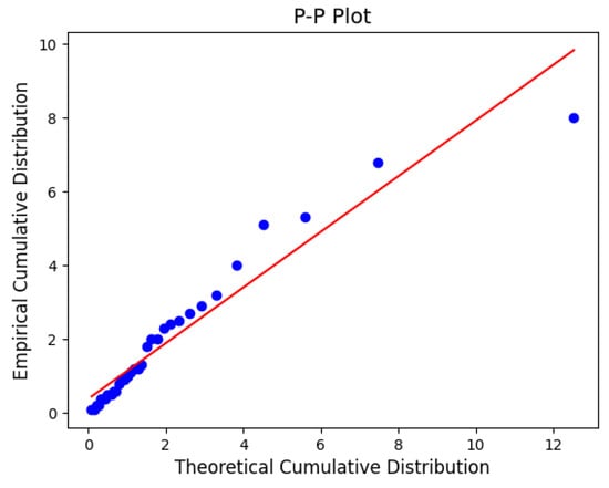
Figure 3. PP-plot for ITL fit to Dataset 1.

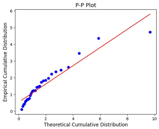
Figure 4. PP-plot for ITL fit to Dataset 2.

Information Criteria and Their Interpretation

AIC.

Akaike Information Criterion: ${\displaystyle \mathrm{AIC}=-2\mathrm{LL}+2k}$.

Balances in-sample fit (LL) with a $2k$ penalty for complexity. A lower AIC indicates better future predictive ability (in the Kullback–Leibler sense).

BIC.

Bayesian Information Criterion (Schwarz): ${\displaystyle \mathrm{BIC}=-2\mathrm{LL}+klnn}$.

Stronger penalty increasing with $lnn$. Favors simpler models as n increases; it is consistent (selects the “true” model if it is among the candidates).

HQIC.

Hannan–Quinn Information Criterion: ${\displaystyle \mathrm{HQIC}=-2\mathrm{LL}+2kln\left(lnn\right)}$.

Intermediate penalty between AIC and BIC. Also consistent, but less strict than BIC for moderate sample sizes; useful when AIC overfits and BIC is too conservative.

10.2. Results

10.2.1. Dataset 1

The following data set represents Vinyl chloride data from clean up gradient ground-water monitoring wells in $\mathsf{\mu }$g/L (Table 3). This is data set was first recorded by Bhaumik et al. [35]:

Table 3. Vinyl chloride concentrations ($\mathsf{\mu }$g/L).

5.1	1.2	1.3	0.6	0.5	2.4	0.5	1.1	8.0	0.8	0.4	0.6
0.9	0.4	2.0	0.5	5.3	3.2	2.7	2.9	2.5	2.3	1.0	0.2
0.1	0.1	1.8	0.9	2.0	4.0	6.8	1.2	0.4	0.2

Table 4 summarizes the fits. The ITL distribution emerges as the preferred model according to the AIC criterion, outperforming both the Inverse Weibull and Inverse Gamma distributions. Specifically, ITL improves upon the Inverse Weibull by $\Delta \mathrm{AIC}=96.7512-87.4843=9.27$, and over the Inverse Gamma by $\Delta \mathrm{AIC}=95.0147-87.4843=7.53$. This indicates a substantially better fit, with ITL capturing the tail behavior more accurately (see Figure 3).

Table 4. Comparison of distributions (Dataset 1).

Model	Log-Likelihood	AIC	BIC	CAIC	HQIC
ITL	−55.5384	115.0768	118.1295	120.1295	116.1179
Inverse Weibull	−58.6266	121.2532	124.3059	126.3059	122.2942
Inverse Gamma	−59.0659	122.1319	125.1846	127.1846	123.1793

10.2.2. Dataset 2

The following data shows the time between failures for 30 repairable items and has been provided by Murthy et al. [36]. The data are listed as follows (Table 5):

Table 5. Time between failures for 30 repairable items.

1.43	0.11	0.71	0.77	2.63	1.49	3.46	2.46	0.59	0.74	1.23	0.94
4.36	0.40	1.74	4.73	2.23	0.45	0.70	1.06	1.46	0.30	1.82	2.37
0.63	1.23	1.24	1.97	1.86	1.17	0	0	0	0	0	0

Table 6 summarizes the comparative goodness-of-fit results for Dataset 2. According to the AIC criterion, the ITL distribution provides the best fit, with the lowest AIC value of 115.08. It outperforms the Inverse Weibull distribution by a margin of $\Delta \mathrm{AIC}=121.25-115.08=6.17$, and the Inverse Gamma distribution by $\Delta \mathrm{AIC}=122.13-115.08=7.05$. These differences indicate that ITL captures the structure of the data more effectively, providing a better balance between fit quality and model complexity. Similar conclusions are supported by BIC, CAIC, and HQIC values. For a visual assessment, refer to Figure 4.

Table 6. Comparison of distributions (Dataset 2).

Model	Log-Likelihood	AIC	BIC	CAIC	HQIC
ITL	−41.742142	87.484284	90.286679	92.286679	88.380794
Inverse Weibull	−46.375609	96.751218	99.553612	101.553612	97.647728
Inverse Gamma	−45.507345	95.014690	97.817085	99.817085	95.911201

Probability–Probability (PP) plots are graphical tools used to assess the goodness-of-fit of a statistical model. They compare the empirical cumulative distribution function (ECDF) of the observed data against the theoretical cumulative distribution function (CDF) of the proposed model. In a P-P plot, each data point represents a pair $(F_{\mathrm{empirical}}\left(x_i\right),F_{\mathrm{theoretical}}\left(x_i\right))$. If the model fits the data well, the points will lie approximately along the 45-degree reference line, indicating that the empirical and theoretical distributions are closely aligned. Deviations from this line suggest discrepancies between the data and the fitted model, particularly in the tails or center, depending on the curvature and pattern of the deviation.

As can be observed in Figure 3 and Figure 4, the Inverted Topp–Leone (ITL) distribution provides a satisfactory fit to both datasets. The points in both PP plots remain close to the diagonal reference line, demonstrating that the ITL distribution adequately captures the empirical behavior of the data. This visual evidence complements the numerical results reported in Table 4 and Table 6, further supporting the suitability of the ITL model for these data sets.

11. Conclusions

By using the classical method of transformation of variables, we have derived and defined an inverted Topp–Leone distribution (ITLD). This distribution has support on the positive real line and can be applied to lifetime data problems. By using standard definitions and results, several properties of this distribution, the CDF, moments, and Fisher information matrix have been derived. Entropies and estimation of parameters associated with the inverted Topp–Leone distribution (ITLD) have also been considered. The likelihood ratio ordering, which also implies other orderings, has been established. The mathematics involved in the derivation of results is tractable, and therefore the model discussed in this article may serve as an alternative to many existing distributions defined on the positive real line.

The ITLD has proven to be a highly competitive alternative for modeling lifetime and reliability data. In particular, goodness-of-fit comparisons with classical distributions—such as the Inverse Weibull and Inverse Gamma—demonstrated that the ITLD provides superior performance across various datasets, as evidenced by lower values of AIC, BIC, CAIC, and HQIC, as well as better alignment with empirical distributions through PP-plots.

The Maximum Likelihood Estimation (MLE) procedure has been implemented to estimate the parameters $\nu$ and $\xi$ of the ITLD. Simulation studies confirmed the consistency and asymptotic normality of the estimators, while also allowing the computation of biases, mean squared errors, and empirical confidence intervals for different sample sizes.

The proposed methodology for ITLD parameter estimation and simulation provides a robust framework that can be extended to more complex models, including bivariate or regression-based generalizations.

The Method of Moments, Least Squares Estimation, Bayesian Estimation, and a comparative analysis with MLE results can also be undertaken. Goodness-of-fit tests such as Kolmogorov–Smirnov (KS) test, including computation of critical values of the test, can also be considered. Future work is to construct multivariate, matrix variate and complex variate generalizations of the proposed distribution. The construction of bivariate, multivariate, and matrix variate generalizations of the suggested distribution is a future project.

References

- Topp, C.W.; Leone, F.C. A family of J-shaped frequency functions. J. Am. Stat. Assoc. 1955, 50, 209–219. [Google Scholar] [CrossRef]
- Kotz, S.; van Dorp, J.R. Beyond Beta. Other Continuous Families of Distributions with Bounded Support and Applications; World Scientific Publishing Co. Pte. Ltd.: Hackensack, NJ, USA, 2004. [Google Scholar]
- Nadarajah, S.; Kotz, S. Moments of some J-shaped distributions. J. Appl. Stat. 2003, 30, 311–317. [Google Scholar] [CrossRef]
- Kotz, S.; Seier, E. Kurtosis of the Topp-Leone distributions. Interstat 2006, 1, 1–15. [Google Scholar]
- Al-Zahrani, B. Goodness-of-fit for the Topp-Leone distribution with unknown parameters. Appl. Math. Sci. 2012, 6, 6355–6363. [Google Scholar]
- Al-Zahrani, B.; Al-Shomrani, A.A. Inference on stress-strength reliability from Topp-Leone distributions. J. King Saud Univ. Sci. 2011, 24, 73–88. [Google Scholar] [CrossRef]
- Bayoud, H.A. Estimating the shape parameter of the Topp-Leone distribution based on type I censored samples. Appl. Math. 2015, 42, 219–230. [Google Scholar] [CrossRef]
- Bayoud, H.A. Admissible minimax estimators for the shape parameter of Topp- Leone distribution. Commun. Stat. Theory Methods 2016, 45, 71–82. [Google Scholar] [CrossRef]
- Bayoud, H.A. Estimating the shape parameter of Topp-Leone distributed based on progressive type II censored samples. REVSTAT 2016, 14, 415–431. [Google Scholar]
- Genç, A.I. Moments of order statistics of Topp-Leone distribution. Stat. Papers 2012, 53, 117–131. [Google Scholar] [CrossRef]
- Ghitany, M.E.; Kotz, S.; Xie, M. On some reliability measures and their stochastic orderings for the Topp-Leone distribution. J. Appl. Stat. 2005, 32, 715–722. [Google Scholar] [CrossRef]
- MirMostafaee, S.M.T.K.; Mahdizadeh, M.; Aminzadeh, M. Bayesian inference for the Topp-Leone distribution based on lower k-record values. Jpn. J. Ind. Appl. Math. 2016, 33, 637–669. [Google Scholar] [CrossRef]
- Vicari, D.; van Dorp, J.R.; Kotz, S. Two-sided generalized Topp and Leone (TS-GTL) distributions. J. Appl. Stat. 2008, 35, 1115–1129. [Google Scholar]
- Zghoul, A.A. Order statistics from a family of J-shaped distributions. Metron 2010, 68, 127–136. [Google Scholar] [CrossRef]
- Zghoul, A.A. Record values from a family of J-shaped distributions. Statistica 2011, 71, 355–365. [Google Scholar]
- Hassan, A.S.; Elgarhy, M.; Ragab, R. Statistical Properties and Estimation of Inverted Topp-Leone Distribution. J. Stat. Appl. Probab. 2020, 9, 319–331. [Google Scholar] [CrossRef]
- Nagar, D.K.; Zarrazola, E.; Sánchez, L.E. Entropies and Fisher information matrix for extended beta distribution. Appl. Math. Sci. 2015, 9, 398–3994. [Google Scholar] [CrossRef]
- Miller, A.R. Remarks on a generalized beta function. J. Comput. Appl. Math. 1998, 100, 23–32. [Google Scholar] [CrossRef][Green Version]
- Jones, M.C. Kumaraswamy’s distribution: A beta-type distribution with some tractability advantages. Stat. Methodol. 2009, 6, 70–81. [Google Scholar]
- Bain, L.J.; Engelhardt, M. Introduction To Probability and Mathematical Statistics; Duxbury: Pacific Grove, CA, USA, 1987. [Google Scholar]
- Prudnikov, A.P.; Brychkov, Y.A.; Marichev, O.I. Integrals and Series. More Special Functions; Gould, G.G., Translator; Gordon and Breach Science Publishers: New York, NY, USA, 1990; Volume 3. [Google Scholar]
- Nagar, D.K.; Zarrazola, E.; Echeverri-Valencia, S. Bivariate Topp-Leone family of distributions. Int. J. Math. Comput. Sci. 2022, 17, 1007–1024. [Google Scholar]
- Masoom Ali, M.; Woo, J. Inference on reliability P(Y < X) in a p-dimensional Rayleigh distribution. Math. Comput. Model. 2005, 42, 367–373. [Google Scholar] [CrossRef]
- Kotz, S.; Lumelskii, Y.; Pensky, M. The Stress-Strength Model and Its Generalizations. Theory and Applications; World Scientific Publishing Co., Inc.: River Edge, NJ, USA, 2003. [Google Scholar]
- Shannon, C.E. A mathematical theory of communication. Bell System Tech. J. 1948, 27, 379–423, 623–656. [Google Scholar] [CrossRef]
- Rényi, A. On measures of entropy and information. In Proceedings of the 4th Berkeley Symposium Mathematical Statistics and Probability, Berkeley, CA, USA, 20 June–30 July 1960; University of California Press: Berkeley, CA, USA, 1961; Volume 1, pp. 547–561. [Google Scholar]
- Nadarajah, S.; Zografos, K. Expressions for Rényi and Shannon entropies for bivariate distributions. Inform. Sci. 2005, 170, 173–189. [Google Scholar]
- Zografos, K.; Nadarajah, S. Expressions for Rényi and Shannon entropies for multivariate distributions. Stat. Probab. Lett. 2005, 71, 71–84. [Google Scholar] [CrossRef]
- Zografos, K. On maximum entropy characterization of Pearson’s type II and VII multivariate distributions. J. Multivar. Anal. 1999, 71, 67–75. [Google Scholar]
- Bapat, R.B.; Kochar, S.C. On likelihood-ratio ordering of order statistics. Linear Algebra Appl. 1994, 199, 281–291. [Google Scholar][Green Version]
- Belzunce, F.; Martínez-Riquelme, C.; Mulero, J. An Introduction to Stochastic Orders; Elsevier/Academic Press: Amsterdam, The Netherlands, 2016. [Google Scholar]
- Boland, P.J.; El-Neweihi, E.; Proschan, F. Applications of the hazard rate ordering in reliability and order statistics. J. Appl. Probab. 1994, 31, 180–192. [Google Scholar]
- Nanda, A.K.; Shaked, M. The hazard rate and the reversed hazard rate orders, with applications to order statistics. Ann. Inst. Stat. Math. 2001, 53, 853–864. [Google Scholar] [CrossRef]
- Shaked, M.; Shanthikumar, J.G. Stochastic Orders; Springer Series in Statistics; Springer: New York, NY, USA, 2007. [Google Scholar]
- Bhaumik, D.K.; Kapur, K.; Gibbons, R.D. Testing parameters of a gamma distribution for small samples. Technometrics 2009, 51, 326–334. [Google Scholar] [CrossRef]
- Murthy, D.N.P.; Xie, M.; Jiang, R. Weibull Models; John Wiley & Sons: Hoboken, NJ, USA, 2004. [Google Scholar]
- Luke, Y.L. The Special Functions and Their Approximations; Academic Press: New York, NY, USA, 1969; Volume 1. [Google Scholar]
- Srivastava, H.M.; Karlsson, P.W. Multiple Gaussian Hypergeometric Series; John Wiley & Sons: New York, NY, USA, 1985. [Google Scholar]
- Johnson, N.L.; Kotz, S.; Balakrishnan, N. Continuous Univariate Distributions-2, 2nd ed.; John Wiley & Sons: New York, NY, USA, 1994. [Google Scholar]
- Gupta, A.K.; Nagar, D.K. Matrix Variate Distributions; Chapman & Hall/CRC: Boca Raton, FL, USA, 2000. [Google Scholar]
Disclaimer/Publisher’s Note: The statements, opinions and data contained in all publications are solely those of the individual author(s) and contributor(s) and not of MDPI and/or the editor(s). MDPI and/or the editor(s) disclaim responsibility for any injury to people or property resulting from any ideas, methods, instructions or products referred to in the content. |
© 2025 by the authors. Licensee MDPI, Basel, Switzerland. This article is an open access article distributed under the terms and conditions of the Creative Commons Attribution (CC BY) license (https://creativecommons.org/licenses/by/4.0/).