


Abstract
Precise rainfall-runoff modeling (RRM) is vital for disaster management, resource conservation, and mitigation. Recent deep learning-based methods, such as long short-term memory (LSTM) networks, often struggle with major challenges, including temporal sensitivity, feature selection, generalizability, and hyperparameter tuning. The objective of this study is to develop an accurate and generalizable rainfall–runoff modeling framework that addresses the four aforementioned challenges. We propose a novel RRM framework that integrates transductive LSTM (TLSTM) to capture fine-grained temporal changes, off-policy proximal policy optimization (PPO) combined with Shapley Additive exPlanations (SHAP)-based reward functions for feature selection, an enhanced generative adversarial network (GAN) for online data augmentation, and Bayesian optimization hyperband (BOHB) for efficient hyperparameter tuning. TLSTM uses transductive learning, where samples near the test point are given extra weight, to capture fine-grained temporal shifts. Off-policy PPO contributes to this process by selecting features sensitive to temporal patterns in RRM. Our improved GAN conducts online data augmentation by excluding some gradients, increasing diversity and relevance in synthetic data. Finally, BOHB accelerates hyperparameter tuning by merging Bayesian optimization with the scaling efficiency of Hyperband. We evaluate our model using the Comprehensive Attributes and Meteorology for Large-Sample Studies (CAMELS) dataset under individual and regional scenarios. It achieves Nash–Sutcliffe efficiency (NSE) scores of 0.588 and 0.873, surpassing the baseline scores of 0.548 and 0.830, respectively. The generalizability of our approach was assessed on the hydro-climatic datasets for North America (HYSETS), also yielding improved performance. These improvements indicate more accurate capture of flow dynamics and peak events, supporting a robust and interpretable framework for RRM.
Keywords:
climate change; data augmentation; feature selection; hyperparameter optimization; rainfall-runoff modeling; water resource management MSC:
62M10; 68T07; 86A05
1. Introduction
RRM plays a crucial role in hydrology, particularly in reservoir management, flood forecasting, and water resource planning [1]. However, accurately modeling runoff remains difficult due to the nonlinear and dynamic nature of the process. Factors like rainfall variability, initial soil moisture, terrain, land cover, and infiltration make predictions uncertain. In particular, rapid shifts in rainfall intensity, short-duration storms, and urbanization (e.g., impervious surfaces) can cause sudden runoff peaks and flash floods. These complex and evolving hydrological phenomena underscore the need for improved modeling frameworks that can more effectively capture these dynamics and generalize them [2].
Over the years, a wide range of approaches have been developed, including traditional machine learning methods [3,4,5,6] and deep learning methods [7,8,9,10,11,12,13], to capture the complex, nonlinear, and dynamic nature of the rainfall–runoff process. However, machine learning models often face limitations in handling high-dimensional data and in accurately capturing nonlinear relationships [14]. Deep learning methods are more powerful, but they still face several challenges. These include temporal sensitivity, feature selection, data augmentation, and hyperparameter tuning [7,15]. Such limitations reduce predictive performance and weaken generalizability across different basins and climatic conditions. However, previous studies have rarely tackled these challenges using a single framework where components work together to strengthen overall performance in RRM. This motivates the need for a more advanced deep learning framework for RRM.
Among various deep learning techniques, LSTM networks have shown their effectiveness in applications such as RRM [15,16,17,18], flood forecasting [19,20], and river water level prediction [21,22,23,24]. Notwithstanding their strengths, conventional LSTMs often struggle with temporal sensitivity. They smooth patterns across entire datasets, missing localized variations. For instance, an LSTM may capture seasonal rainfall cycles but fail to detect sudden storms, which leads to underestimated peak flows and poor short-term forecasts in dynamic regions. This limits their reliability in hydrological applications where fine-grained temporal patterns are essential [25]. TLSTM addresses this by adjusting weight updates based on the proximity of new data points, which helps maintain sensitivity to both broad trends and local events. However, TLSTM requires more computation and risks overfitting in low-data scenarios due to its localized focus [26].
Effective feature selection is crucial for RRM because it influences how well the model captures relevant rainfall and runoff patterns, thereby improving prediction accuracy [27]. Traditional methods, such as gradient boosting machines (GBM), random forest (RF), and decision trees (DT), are widely used in RRM [28]. However, they often struggle with high-dimensional, complex data and may fail to model nonlinear relationships that are critical for accurate RRM [29]. These methods are also prone to overfitting, particularly with small or non-diverse datasets. Recent alternatives, such as attention mechanisms, the least absolute shrinkage and selection operator (LASSO) [30], genetic algorithms [31], and advanced metaheuristic algorithms like the slime mold [32] and marine predator [33], offer improvements but face drawbacks such as ignoring context, removing useful features, slow convergence, and poor solution quality, which limit timely and reliable decisions [34].
Sophisticated deep reinforcement learning (DRL) uses advanced reward-based mechanisms to address feature selection challenges in previous methods [35]. It rewards crucial but often overlooked features, thereby improving the ability of the model to detect subtle and important patterns. Incorporating explainable artificial intelligence (XAI), such as SHAP, strengthens feature selection by providing importance scores that help avoid missing influential variables and show why each feature affects predictions. Adding SHAP values to the reward structure guides DRL toward consistently relevant attributes, thereby improving interpretability and producing clearer, more practical models [36]. This supports validation and stakeholder acceptance. However, DRL struggles with sample efficiency due to reliance on on-policy data. Off-policy methods overcome this limitation by reusing past experiences from a replay buffer, enabling broader learning with fewer new samples and thereby boosting efficiency and stability.
Generalizability is essential in RRM to ensure consistent performance across diverse geographic and climatic conditions, enabling broader applicability [37]. Data augmentation is typically categorized as offline or online. Offline methods expand the dataset size and increase computational load and training time, while online augmentation adds new samples to training batches without increasing the dataset size, which reduces storage usage and improves data quality. GANs have improved online augmentation but still face instability and mode collapse, which limits sample diversity. Solutions include supervised GANs with extra classification data, GAN–autoencoder hybrids, and refined loss functions [38]. Still, these struggle with complex RRM data. Our enhanced GAN differs from traditional versions by omitting gradient updates for unstable batch elements, which directly addresses instability and mode collapse. This selective omission enhances the diversity and contextual relevance of generated samples, which is essential for RRM, where fine-grained variability plays a crucial role.
Optimal hyperparameter tuning is essential for achieving high model performance in rainfall–runoff modeling. Incorrect settings may cause overfitting or underfitting, thereby reducing the effectiveness of the model in real-world scenarios [39]. Several strategies address this, including grid search [40], Bayesian optimization [41], evolutionary algorithms [42], and hyperband [43]. Grid search exhaustively explores parameter combinations but is computationally expensive for high-dimensional models. Bayesian optimization utilizes probabilistic models and historical data to explore efficiently, although it may become trapped in local optima. Evolutionary algorithms simulate natural selection but are time-consuming and resource-intensive. Hyperband improves efficiency by focusing resources on promising configurations [44]. BOHB combines the predictive ability of Bayesian optimization with the efficiency of Hyperband, thereby reducing its limitations and providing a scalable solution for hyperparameter tuning in complex RRM tasks [45].
The objective of this paper is to develop a deep learning model for RRM that jointly addresses the key challenges of temporal sensitivity, feature selection, data augmentation, and hyperparameter tuning. To achieve this, we present a framework that integrates TLSTM, off-policy PPO with SHAP, an enhanced GAN, and BOHB. This is the first time such a combination has been used in RRM within a mutually reinforcing structure. TLSTM enhances temporal sensitivity and facilitates improved feature selection through PPO–SHAP. The stabilized GAN enhances data diversity, benefiting both temporal modeling and feature discovery. BOHB jointly tunes all components to maintain stable and high performance.
The critical contributions of our model include:
- TLSTM is designed to detect subtle temporal changes in data, increasing model sensitivity to environmental shifts. Unlike standard LSTM, it improves prediction accuracy, shown by high NSE scores, which supports better disaster management and resource planning.
- Off-policy PPO enhances feature selection by using past experiences to guide decisions. By integrating SHAP into the reward function, it highlights impactful features and improves sample efficiency, enabling accurate and generalizable runoff predictions across varied regions.
- The improved GAN removes less important gradients and generates diverse, relevant training samples without enlarging the dataset. This increases robustness against overfitting and improves generalization, especially when data is scarce, thereby enhancing the real-world reliability of the model.
- BOHB combines the precision of Bayesian optimization with the rapid evaluation of Hyperband to accelerate hyperparameter tuning. It enables fast iteration and performance gains in dynamic environments, such as RRM, ensuring scalability, efficiency, and optimal results for large and complex datasets.
2. Materials and Methods
2.1. Study Area and Dataset
In this paper, we use the CAMELS [46] and HYSETS [47] datasets to evaluate the proposed model. The CAMELS dataset, which comprises data from watersheds across the United States, was selected due to its comprehensive scope and diverse range of hydrological and meteorological attributes. It offers in-depth meteorological and runoff information essential for effective model testing. This approach, with its focus on detailed and diverse data, is adaptable to similar hydrological datasets, ensuring consistent and fair comparisons, as well as thorough evaluations tailored to the specific characteristics of each dataset. CAMELS comprises data from 674 basins, totaling 11,981 data points across the United States. The broad dataset facilitates rigorous model assessment and includes meteorological inputs, watershed features, and documented daily runoff statistics for each basin spanning from 1 October 1980 to 31 December 2014. For specific basin rainfall–runoff simulations, we use daily weather data sourced from Daymet [48]. For regional models, we utilize data from the Maurer dataset [49]. Our selection of diverse meteorological data sources aligns with the benchmarks established for individual and regional rainfall–runoff modeling, which also uses these two distinct datasets. Catchment features, including soil composition, climatic conditions, vegetation cover, and others, are extensively detailed in Table 1, along with meteorological forcings and catchment details. A total of 32 features can be extracted from each record. For individual basin modeling, we mirror the benchmarks by selecting the same 673 basins. Similarly, for regional modeling, we use the same 448 basins as those in benchmark studies. To ensure a fair comparison, our method employs the same daily meteorological forcings and catchment attributes as those used in the benchmarks.
Table 1.
Meteorological forcings and catchment characteristics in the CAMELS dataset.
To assess the generalizability of the proposed model, we utilized the HYSETS dataset, which encompasses data from 14,425 catchments across Canada, the United States, and Mexico. This dataset comprises streamflow records, meteorological forcings, and physiographic catchment attributes, offering a diverse and challenging environment for testing model robustness.
Both CAMELS and HYSETS datasets contained some missing values, especially in precipitation and temperature. We used linear interpolation for gaps shorter than three days. For longer gaps, we applied seasonal mean imputation based on common hydrological methods. All features were normalized to have zero mean and unit variance using statistics from the training data. Runoff values were log-transformed to reduce skewness and stabilize variance. We clipped values that were more than three standard deviations from the mean to prevent learning disruption. These preprocessing steps helped maintain data quality and improve model reliability.
To ensure fair model evaluation and prevent data leakage, each dataset was partitioned into three subsets: 70% for training, 15% for validation, and 15% for testing. This ratio provides enough data for model training. It also offers sufficient unseen samples for reliable validation and testing. The 70% training portion enables the model to learn underlying temporal and spatial hydrological patterns. The 15% validation subset supports guiding early stopping decisions without overfitting. The final 15% reserved for testing ensures an unbiased assessment of generalization to unseen events. This stratified split was applied independently to both the CAMELS and HYSETS datasets to maintain consistency across different climatic and geographical conditions. This partitioning is critical in hydrological time-series modeling. It helps preserve temporal order and prevents future data leakage. These steps simulate real-world use and lead to trustworthy performance metrics.
2.2. Evaluation Metrics
To assess performance, we use the following indicators: NSE, mean square error (MSE), root MSE (RMSE), normalized RMSE (NRMSE), and absolute top 2% prediction error (ATPE-2%) [50]. NSE measures predictive accuracy by comparing predicted runoff to the variability of observed values. It is commonly used in hydrology because values close to 1 show strong agreement. MSE and RMSE capture average squared errors. RMSE is expressed in the same units as the target variable, emphasizing large errors. This feature is important for detecting sudden changes in runoff. NRMSE, computed by dividing RMSE by the mean observed runoff, enables comparison across river basins with differing flow scales. This normalization is critical in multi-watershed modeling. The ATPE-2% focuses on high-flow extremes by measuring errors for the top 2% of runoff values. It is particularly relevant for flood forecasting, reservoir management, and infrastructure planning. Together, these metrics offer a comprehensive assessment of model reliability, sensitivity to extreme events, and adaptability to diverse hydrological contexts. They help ensure that the model performs well not just on average, but also during critical high-risk scenarios.
NSE is calculated using the following formula:
In this equation, represents the observed value at the instance, denotes the predicted value, and is the mean of observations.
MSE and RMSE are defined as follows:
A lower MSE and RMSE indicate a more accurate model.
NRMSE is the normalized version of RMSE, allowing models to be compared across different scales. It is computed as follows:
where and correspond to the maximum and minimum observed values, respectively. A smaller value of NRMSE reflects higher predictive precision of the model.
ATPE-2% evaluates the precision of peak flow forecasts and is defined as follows:
Here, , with being the -ordered runoff observation, as its prediction, and as the count of top 2% peak observations. A smaller ATPE-2% value signifies a superior model.
2.3. Model Overview
This paper presents an innovative approach for developing a rainfall–runoff model using an off-policy PPO for feature selection, an enhanced GAN for online data augmentation, and the BOHB algorithm for precise hyperparameter tuning. As illustrated in Figure 1, the DRL strategy integrates a TLSTM model with a multilayer perceptron (MLP). The procedure starts with the input variables going through several TLSTM layers. The output from the final TLSTM layer is then fed into an MLP network. This MLP is designed to generate outputs, where represents the number of features equivalent to the number of input variables. The off-policy PPO algorithm is used to train both the TLSTM and MLP models to select features and make predictions.
Figure 1.
Schematic of the proposed RRM model integrating TLSTM for temporal modeling, off-policy PPO with SHAP for feature selection, improved GAN for online augmentation, and BOHB for hyperparameter tuning. All components interact in a mutually reinforcing structure.
2.3.1. Online Data Augmentation
Data augmentation enhances the flexibility of deep neural networks by generating diverse data samples, thereby helping to prevent overfitting and increase robustness, particularly when data is scarce. This technique trains models to detect various features, enhancing their effectiveness in real-world settings. It is crucial in RRM, where acquiring large, labeled datasets is difficult. Data augmentation methods are categorized into two types: offline and online. Offline data augmentation enlarges and processes datasets before training, requiring substantial storage and extending loading periods. This rigid method may create duplicate data and increase the risk of overfitting because the same augmented samples are used repeatedly. Conversely, online data augmentation dynamically generates data during training, enhancing the generalization ability of the model and reducing the need for large storage.
This paper introduces a GAN-based online data augmentation method that selectively excludes gradients from key batch elements, helping the model produce more varied and applicable results. The detailed procedures of this online data augmentation method are outlined in Algorithm 1. The generator and discriminator in our GAN include a TLSTM model followed by an MLP for prediction. The discriminator in our GAN component used the binary cross-entropy (BCE) loss function, as it showed stable convergence during adversarial training.
| Algorithm 1 Pseudo-code for online data augmentation algorithm |
| Input: : defined probability threshold for keeping a sample, : number of minibatches Output: Expanded dataset Begin with initializing initial batches Assign as an empty collection for each in : Compute the retention probability for each sample in for each sample in : if < // is the probability of retaining sample I Move to the next sample (omit any modifications) else: Determine y, the label of the sample I Generate a new sample with the same label Substitute the sample I with the newly created sample Append the possibly modified to return the augmented batch set |
The Proposed Generator
GANs comprise two interconnected networks that learn in parallel: the generator and the discriminator. The generator creates fake outputs that mimic real data, while the discriminator strives to improve the results of the generator. Together, these networks engage in a competitive min-max game, employing a value function as described below [51]:
where and correspond to the input data and random noise, respectively. and represent the generator and discriminator. and illustrate the probability distributions of the input data and noise, respectively. and are the expected value and logarithm, respectively. In this research, the generator implements a unique training approach that differentiates it from traditional generators. Notably, when updating the parameters of the generator with a generated mini-batch, gradients from those mini-batch elements that yield the most significant effects are omitted. This novel approach to updating the generator is detailed as follows:
Here, indicates how the discriminator evaluates each element in the mini-batch . represents the set of parameters for the generator, and indicates the learning rate for the generator. ∑〗 aggregates the responses of the discriminator to the top-k most impactful elements in the mini-batch . Furthermore, represents the gradient of the value function concerning the parameters of the generator. During the training process, the discriminator evaluates the outputs generated by the generator. Outputs that closely match the target distribution receive high ratings, while those that differ greatly are rated lower. The updates to the generator are influenced by the highest-rated samples as judged by the discriminator in each batch.
Omitting gradients from mini-batch elements that trigger the strongest discriminator responses is a strategic way to overcome common GAN training issues. This prevents the generator from overemphasizing dominant features that may not generalize well, helping it capture a broader range of patterns. The approach stabilizes training and reduces mode collapse, where the generator produces repetitive outputs with limited diversity. Skipping the strongest gradients enables the generator to produce a wider range of outputs, which in turn helps make the model more robust and effective across various inputs.
2.3.2. Feature Engineering and Prediction
Let us consider a dataset D consisting of pairs , where is a vector with input variables , and is the corresponding outcome. Each cycle randomly chooses a pair from D, with the agent deciding which variables to use. In our DRL setup, the state space S includes the data point , outcome , and the selected variables . The actions in our framework are part of the set , which includes choosing a variable or making a decision . Choosing a variable from expands the set of variables , altering the space for predictions. The reward for selecting a variable is defined by , where is the SHAP value for the variable and is a tuning hyperparameter. Actions culminating in predictions transition the model to an endpoint, resulting in rewards or penalties calculated by , where MSE measures the mean squared error between the actual () and predicted () values. Thus, is formally established to express these dynamics:
Using SHAP values in the reward mechanism of a DRL model for RRM is crucial for enhancing model interpretability and precision. SHAP values quantify the impact of each input feature on the predictions of the model, allowing for a more targeted and efficient learning process. Integrating SHAP values enables the DRL model to focus on the features that have the most significant impact on predictions, thereby improving accuracy and overall model performance. This method helps mitigate overfitting and enhances the ability of the model to generalize to new data scenarios, making it indispensable in environments where understanding the contribution of individual features is key to making informed decisions.
The transition function of the model operates as described below:
where denotes the final state. Whenever an action involves selecting an additional feature, this feature is added to the set . The episode ends when the agent decides to make a prediction. Acknowledging that our DRL model operates within a discrete-time setting is important. The time variable in and indicates when decisions to add features occur. Each decision or time step entails choosing a feature that may enhance the accuracy of future predictions, thus influencing subsequent states and rewards. This ongoing decision-making sequence is crucial to DRL, distinguishing it from static supervised learning models, where the features are fixed and not adaptively refined.
The pseudocode outlined in Algorithm 2 illustrates how the model applies feature extraction and prediction to execute its learning approach. This process includes randomizing the dataset, selecting actions that align with the existing strategy, executing these actions within the structure of the model, and modifying the strategy in response to feedback and alterations in state. The off-policy PPO algorithm is employed to enhance policy training.
| Algorithm 2 Pseudo-code for training the proposed model. |
| Input: Data = , learning rate α, epochs E Initialize policy parameters and old policy parameters Initialize value function parameters Initialize advantage estimator Establish initial replay buffer Initialize Q-function with random weights for to : Randomize order of for to : Select action with probability Set initial state Perform action Calculate the reward using Equation (8) Determine next state from Store transition (,,,) in Compute using value function parameters Update policy optimize the objective function via Equation (15): |
Training
To improve policy training, the DRL framework uses an off-policy PPO algorithm. In this section, we first explore trust region policy optimization (TRPO) and then discuss PPO, which lays the groundwork for off-policy PPO. Finally, we present the off-policy PPO method.
- TRPO
In DRL, the aim is to determine a policy π that yields the highest possible total of future rewards:
In this setup, signifies that the starting state is sampled from an initial distribution. The policy π(at|st) expresses the likelihood of choosing action at in state st, while captures the dynamics of moving to the next state. The discount rate determines the extent to which future outcomes influence current decisions. TRPO refines the policy by optimizing a proxy objective, constrained by a Kullback–Leibler (KL)-divergence bound to prevent large shifts between policy iterations:
In this formulation, indicates that the initial state is drawn from a starting distribution. The policy defines the action probabilities in each state, and the transition function models the probability of moving to the next state given the current state and action. The discount factor adjusts the importance of future rewards. TRPO updates the policy by maximizing a surrogate objective while limiting policy shifts through a Kullback–Leibler (KL) constraint:
subject to
Here, represents the existing policy, and defines the threshold for divergence. calculates the KL divergence, evaluating how much the policy deviates from the previous policy at a specific state . denotes the discounted state distribution resulting from the initial state under the old policy , expressed as . However, without this divergence constraint, optimizing the surrogate objective function, as defined in Equation (12), may lead to significant alterations in the policy.
- PPO
PPO maintains update stability by optimizing a modified surrogate loss with clipping constraints:
The constant is a small positive value that controls the trade-off between safe updates and exploration. The advantage term measures how much better an action is compared to the average under the previous policy. Clipping the ratio limits drastic policy updates and stabilizes the learning process:
In this context, represents the value being modified, with a and b denoting the lower and upper bounds, respectively, within which is constrained. This formulation discourages updates where the likelihood ratio stays too far from unity. Despite its strengths, PPO has a notable drawback: it depends primarily on on-policy sampling. This reliance results in high sample inefficiency, as the agent must frequently interact with the environment. Such repeated engagement increases the overall computational demands during training.
- Off-policy PPO
This study introduces off-policy PPO for training the policy of the feature selection and prediction. It improves sample efficiency by utilizing prior experiences and diverse policy decisions. Off-policy PPO benefits from a broader dataset. In contrast, standard on-policy PPO relies heavily on recent interactions and needs a large volume of fresh data. This broader dataset encompasses historical records and diverse decision-making strategies. For example, it can use rainfall–runoff records collected over decades from multiple regions. This helps the model learn from a wider range of flood events and scenarios that are not present in recent data. It also enables evaluation of long-term conservation strategies, refining models for adaptive and accurate forecasting. This is crucial in RRM, where evolving environmental conditions and human actions necessitate models that can adapt quickly and effectively.
The off-policy PPO approach updates the policy using historical data generated by a behavior policy, denoted as , rather than data sampled from the current policy . PPO limits the size of policy updates by clipping the probability ratio between the current policy and the behavior policy. This prevents unstable learning caused by large, sudden changes. This ensures the policy update remains within a controlled region.
The final surrogate objective used for updating the feature selection policy, which is inspired by the off-policy TRPO, is as follows:
where , , , , and .
Off-policy PPO increases the selection likelihood of features that produce higher rewards. Features that consistently yield higher advantage values in accurate runoff estimation contribute strongly to accurate runoff estimation. Off-policy PPO reinforces its reuse during later updates. In contrast, features linked to lower rewards lose selection probability over time, allowing the model to discard less useful variables. Off-policy PPO repeatedly updates the policy to keep only features that reliably improve prediction accuracy. This makes the feature selection process adaptive, data-efficient, and robust, without requiring extra assumptions about state or action definitions.
Figure 2 illustrates the step-by-step optimization process of the feature selection policy using the off-policy PPO algorithm. The process begins by defining the optimization problem using off-policy data, enabling the model to benefit from prior experience. The method introduces a clipped surrogate objective. This ensures stable and gradual policy updates through a clipping strategy. The clipped objective is adapted to suit off-policy data. The next step involves evaluating the policy ratio to control divergence from earlier policies. A correction factor is applied to refine and stabilize updates. The policy is then updated, and the process checks for termination. If not met, the cycle continues. This approach improves stability, efficiency, and generalization across hydrological modeling tasks.
Figure 2.
Seven-step optimization process of the feature selection policy using off-policy PPO.
2.3.3. Hyperparameter Optimization
BOHB enhances the process of hyperparameter tuning by integrating the probabilistic modeling strength of BO with the adaptive resource allocation of HB. Utilizing the tree-structured Parzen estimator (TPE) from BO, BOHB estimates the likelihood of performance success, allowing it to differentiate between highly promising and less effective hyperparameter choices. This forecasting capability improves the efficiency of the search compared to standard techniques such as random or grid search. Using the early-stopping strategy of HB, BOHB allocates more computational resources to the most promising candidates while reducing expenditure on underperforming options.
By fusing the probabilistic modeling accuracy of BO with the adaptive resource management of HB, BOHB offers a powerful mechanism for efficiently exploring complex hyperparameter spaces. It adeptly maintains a trade-off between testing novel parameter combinations and refining known effective ones while directing computational effort toward the most favorable candidates. This methodology makes BOHB especially advantageous in scenarios with constrained computational budgets and intricate tuning requirements, delivering a reliable and scalable approach for addressing the complexities of hyperparameter optimization in advanced machine learning tasks.
Figure 3 illustrates the full workflow of the proposed RRM model. It begins with preprocessing to clean missing data and normalize inputs between 0 and 1. Next, BOHB proposes sets of hyperparameters, tests model performance with each set, and refines the distribution repeatedly until the results stabilize. Once optimal hyperparameters are found, a GAN is trained for online data augmentation and saved. The trained GAN then produces synthetic samples to enrich the training set. TLSTM performs feature extraction from the augmented data, capturing temporal dependencies in time-series runoff data. Off-policy PPO is used to select relevant features. This method adapts input selection over time through the use of reinforcement learning. This cycle continues until the PPO meets its stopping criteria. Finally, the generalization of the model is assessed on the test set. This workflow ensures robust training, dynamic feature optimization, and improved forecasting accuracy in hydrological scenarios.
Figure 3.
Overall flowchart of the proposed model.
3. Results and Discussion
The study was conducted on a 64-bit Windows operating system equipped with an Intel Core i7 processor and 32 gigabytes (GB) of random-access memory (RAM), ensuring sufficient computational power for complex model training and data processing. We utilized Python 3.8 as the software framework due to its extensive library support and strong community, which is particularly beneficial for machine learning tasks. Key libraries included PyTorch 1.13.1, which was used to construct and train deep learning models, such as our TLSTM and enhanced GAN. We implemented the off-policy PPO and BOHB algorithms using the Python libraries stable-baselines and HpBandSter, respectively. This setup enabled the integration of sophisticated machine learning techniques and optimization algorithms to effectively tackle the challenges in RRM, improving the accuracy and applicability of the model across various hydrological datasets, such as CAMELS.
To evaluate the robustness and accuracy of our models, we implemented a 5-fold stratified cross-validation method. This technique is particularly effective in ensuring that each data fold represents the whole, thereby maintaining the distribution of different rainfall–runoff events across all folds. Stratified cross-validation is crucial for RRM because it accounts for variations in weather patterns and hydrological responses, preventing model overfitting and ensuring consistent performance across diverse datasets. This approach enhances the reliability of the evaluation by minimizing bias and variance in the performance predictions of the model.
Table 2 presents the hyperparameters optimized using the BOHB method. We assessed our innovative algorithm against fourteen recent methods published in the last two years: four machine learning models, including GEP [3], Wavelet-hybrid [4], MLP-ensemble [5], Bayesian-regionalization [6]; and ten deep learning models, including CNN-LSTM [2], Transformer-LSTM [15], EA-LSTM [7], CNN-RNN [8], Transformer [9], AI-Based [10], and Self-training [11], GAN-TLSTM [25], Hybrid-ensemble [12], and Frequency-CNN [13]. The results for all these techniques are obtained from the implementations provided by their respective authors. We conducted both individual and regional rainfall–runoff modeling to predict runoff for lead times of 1, 2, 4, and 8 days. Results for individual modeling are presented in Table 3, Table 4, Table 5 and Table 6, while those for regional modeling are presented in Table 7, Table 8, Table 9 and Table 10.
Table 2.
Optimized hyperparameters for the proposed runoff prediction model.
Table 3.
Comparative analysis of runoff prediction models over a 1-day forecast horizon in individual modeling.
Table 4.
Comparative analysis of runoff prediction models over a 2-day forecast horizon in individual modeling.
Table 5.
Comparative analysis of runoff prediction models over a 4-day forecast horizon in individual modeling.
Table 6.
Comparative analysis of runoff prediction models over an 8-day forecast horizon in individual modeling.
Table 7.
Comparative analysis of runoff prediction models over a 1-day forecast horizon in regional modeling.
Table 8.
Comparative analysis of runoff prediction models over a 2-day forecast horizon in regional modeling.
Table 9.
Comparative analysis of runoff prediction models over a 4-day forecast horizon in regional modeling.
Table 10.
Comparative analysis of runoff prediction models over an 8-day forecast horizon in regional modeling.
In individual modeling, among the machine learning models, the Bayesian-regionalization outperformed GEP, Wavelet-hybrid, and MLP-ensemble, with approximately 6.1%, 5.4%, and 4.2% higher NSE for 8-day forecasts, respectively. However, although Bayesian-regionalization achieved a slightly higher NSE, its RMSE was noticeably higher than that of deep learning models such as CNN-LSTM and Transformer-LSTM. The elevated MSE values for Bayesian-regionalization also confirm its tendency to produce larger squared errors, indicating challenges in minimizing overall variance in predictions. This suggests that despite better NSE values, it struggled to minimize prediction errors effectively. Comparing hybrid models, Transformer-LSTM improved RMSE over CNN-LSTM by about 6.7% for 8-day forecasts. EA-LSTM further enhanced NSE by 4.3% compared to Transformer-LSTM. CNN-RNN outperformed EA-LSTM by 1.6% in RMSE for 4-day-ahead forecasts, though it lagged behind Transformer in NSE by about 2.1% for 1-day-ahead forecasts. Notably, CNN-RNN also exhibited lower NRMSE scores than EA-LSTM, highlighting its advantage in producing scale-independent and consistent performance. AI-based and Self-training models maintained better RMSE scores than CNN-LSTM by 9.8% and 12.5% for the 8-day-ahead forecast, respectively, showcasing their improvements in error control. This improvement was also reflected in lower MSE and NRMSE values, reinforcing their generalization ability across varying runoff magnitudes. Hybrid-ensemble achieved a further 2.4% enhancement in NSE over Self-training for 1-day-ahead forecasting. Frequency-CNN delivered the best overall performance among deep learning models prior to the proposed method, improving RMSE by 3.8% over Hybrid-ensemble for a 1-day ahead forecast and securing a 5.1% advantage in NSE. It also showed reduced NRMSE and MSE values, reflecting both precision and consistency. However, across the longer forecast horizons (8 days), Frequency-CNN still had a larger RMSE compared to the proposed model. The proposed model also achieved the lowest NRMSE and MSE across most timeframes. This indicates its stronger generalization capability, with reduced prediction variance and more accurate scale-normalized performance.
In regional modeling, the CNN-RNN model reduced RMSE by 13.5% compared to EA-LSTM for 4-day-ahead forecasts; however, it did not achieve similar improvements in NSE. The Transformer achieved a 7.2% improvement in NSE over CNN-RNN for 2-day-ahead forecasting. Meanwhile, AI-Based and Self-training models demonstrated substantial robustness, boosting NSE by 3.6% and 4.9% over Transformer for 4-day-ahead horizons. Frequency-CNN, once again, marked the best benchmark performance, outperforming Hybrid-ensemble with 2.1% better NSE for 1-day-ahead and reducing RMSE by 6.4% for 8-day-ahead. However, Frequency-CNN had weaknesses in predicting extreme values based on ATPE-2%, and showed only moderate results in both MSE and NRMSE. For example, its average NRMSE over all four forecast horizons was 0.156, and the mean MSE was 2.489. These results suggest that there is still potential to improve consistency in prediction errors. Thus, although state-of-the-art models demonstrated progressive improvements, none consistently outperformed others across RMSE, NSE, MSE, NRMSE, and ATPE-2% for all forecast horizons. This inconsistency highlights a major limitation.
The proposed model consistently outperformed all existing models across individual and regional modeling settings. In individual modeling, the proposed model outperformed Frequency-CNN at the 1-day-ahead horizon, achieving a 17.8% lower RMSE, a 14.3% higher NSE, and a 32.6% better ATPE-2%. At the 8-day horizon, improvements were even more notable, with the RMSE decreasing by 9.7%, the NSE increasing by 26.0%, and the ATPE-2% decreasing by 34.8% compared to Frequency-CNN. Compared to Self-training, the proposed model achieved a 36.5% lower RMSE, a 20.5% higher NSE, and a 58.2% lower ATPE-2% for 1-day-ahead predictions. The proposed model showed 34.6% lower RMSE and 18.5% higher NSE than AI-Based at the 8-day forecast horizon. Similarly, compared to Transformer, improvements of 33.3% in RMSE and 22.4% in NSE were achieved for 4-day-ahead forecasts. Compared to GAN-TLSTM, our previous model, the proposed approach demonstrated consistent and substantial gains across all forecast horizons. For example, at the 1-day horizon, RMSE and ATPE-2% were reduced by 34.2% and 51.6%, respectively, while NSE improved by 10.1%. These improvements show that although GAN-TLSTM included spatial attention, GAN-based data reduction, and DE for tuning, it did not use a dynamic feature selection method or a flexible process like BOHB.
In regional modeling, the proposed model achieved remarkable performance improvements across all five key metrics. At the 1-day forecast horizon, the proposed model reduced RMSE by 53.2%, MSE by 56.0%, and NRMSE by 34.5% compared to Frequency-CNN. It also lowered ATPE-2% by 71.0% and improved NSE by 2.8%. For the 2-day horizon, it outperformed self-training by 29.6% in RMSE, 21.6% in MSE, and 29.9% in NRMSE. It also reduced ATPE-2% by 55.7% and increased NSE by 7.6%. At the 4-day horizon, the proposed model outperformed AI-Based by reducing RMSE by 24.5%, MSE by 42.1%, NRMSE by 24.9%, and ATPE-2% by 56.3%. It also improved NSE by 4.6%. At the 8-day horizon, the model reduced RMSE by 27.5%, MSE by 38.3%, and NRMSE by 21.3% compared to Transformer. It also achieved an 88.4% reduction in ATPE-2% and a 4.9% increase in NSE. Against GAN-TLSTM at the 1-day horizon, the proposed model reduced RMSE by 27.0%, MSE by 60.4%, and ATPE-2% by 55.8%. It also improved NSE by 3.0%.
The superior performance of the proposed model has clear implications for practical hydrological applications. The consistent reduction in RMSE and NRMSE indicates more reliable estimates of daily runoff volumes. This improvement supports more effective reservoir operations and informed short-term water allocation decisions. The substantial gains in NSE reflect a stronger ability to track rapid hydrological fluctuations. As a result, the model becomes more effective for issuing early flood warnings and responding to emergencies. The significant reductions in ATPE-2% demonstrate improved handling of extreme runoff events. These events are often crucial for ensuring infrastructure safety, effective dam operations, and mitigating downstream risks. In regional settings, the model remained stable across heterogeneous basins. This suggests it can generalize well to ungauged or data-scarce catchments. It is therefore suitable for large-scale hydrological forecasting systems. Overall, these improvements show that the proposed approach is not only more accurate but also more robust and operationally dependable for real-world water management scenarios.
We conducted paired t-tests across NSE, MSE, RMSE, NRMSE, and ATPE-2% metrics to assess the statistical significance of the superiority of our model. In individual modeling, the p-values remained consistently below 0.001 when compared to the next-best model. The 95% confidence intervals further validated these improvements: NSE ranged between [0.048, 0.075], MSE between [−0.92, −0.52], RMSE between [−0.72, −0.46], NRMSE between [−0.43, −0.12], and ATPE-2% between [−0.22, −0.17]. In regional modeling, p-values were under 0.0005, with similar confidence intervals. Additionally, effect size analysis (Cohen’s d > 1.2) demonstrated that the improvements were not only statistically significant but also practically meaningful, reinforcing the robustness of our model across RRM tasks.
Table 11 illustrates a direct comparison of the computational efficiency of rainfall–runoff models based on their runtime and GPU consumption. Our proposed model achieves a runtime of 4326 s and a GPU usage of 18.3 GB. Compared to Frequency-CNN, our model is approximately 4.3% faster and reduces GPU usage by 5.7%. Against Hybrid-ensemble, it is 7.7% faster with a 10.7% reduction in GPU usage. For GAN-TLSTM, the model improves runtime by 13.0% and lowers GPU usage by 15.7%. In contrast, Transformer-LSTM outperforms our model on both metrics (4156 s vs. 4326 s, ~4.1% faster; 15.2 GB vs. 18.3 GB, our model uses ~20.4% more GPU). Compared with Self-training, our runtime is lower by ~17.5% (5245 s vs. 4326 s), but our GPU memory is higher by ~9.6% (16.7 GB vs. 18.3 GB). Overall, the model offers a balanced trade-off between speed and memory efficiency, outperforming several resource-heavy baselines. However, it does not surpass optimized models such as Transformer-LSTM in either metric.
Table 11.
Comparative analysis of runtime and GPU usage metrics across rainfall–runoff models.
Figure 4 traces the trajectory of loss values over 300 epochs during the training and validation stages. The graph shows that training and validation losses steadily decrease, suggesting that the proposed model converges effectively. Moreover, the gap between the training and validation curves remains consistently small across epochs. This consistency indicates that the model generalizes well and avoids significant overfitting. Stabilizing both losses toward the end further suggests that the model achieves reliable performance and robust optimization.
Figure 4.
Loss trajectory over 300 epochs for training and validation stages.
Figure 5 illustrates the decision time distributions of the proposed model, offering important insight into its usability in real-time systems. The decision-making times fall within a narrow range of 50 ms to 75 ms. The peak frequency is observed to be around 62 ms. This narrow range and low latency indicate that the model processes inputs rapidly and consistently, minimizing delays in critical operations. This rapid and stable decision-making is particularly critical when quick predictions are vital during extreme events. The consistent sub-70 ms response time confirms the readiness of the model for practical deployment in real-world hydrological monitoring and emergency management systems.
Figure 5.
Decision-making time distributions for the proposed model.
To further demonstrate the effectiveness of our proposed model, we present a case study on regional rainfall–runoff modeling, depicted in Figure 6. This figure illustrates the performance of the model over one year, from 1 January 2013 to 1 January 2014, providing a comprehensive view of its predictive capabilities. The graph compares the observed runoff and the predicted runoff of the model for the specified period. The close alignment between the observed (solid blue line) and predicted (dashed red line) runoff curves highlights the strong predictive performance of the model. The model accurately captures seasonal fluctuations and peak flow events, with minimal deviation during critical runoff periods such as early spring and late autumn. Moreover, the model maintains consistent accuracy across low and moderate flow conditions. It effectively avoids both underestimation and overestimation during these periods. These results confirm the robustness of the proposed model and its ability to generalize well across varying hydrological conditions, making it highly reliable for real-world regional runoff forecasting applications.
Figure 6.
Regional rainfall–runoff modeling from 1 January 2013 to 1 January 2014, comparing observed and predicted runoff.
3.1. Ablation Studies
This section assesses the performance of the model by removing critical components to observe their effects on overall effectiveness. The ablation study involved excluding TLSTM, feature selection (FS), off-policy PPO, SHAP, the improved GAN for online data augmentation, and hyperparameter optimization (HO). The corresponding results are shown in Table 12.
Table 12.
Impact of component removal on model performance metrics through ablation studies.
Compared to the full model, removing TLSTM resulted in an increase of 35.5% in RMSE, a 35.8% rise in NRMSE, and a 38.5% decrease in NSE. These results highlight the importance of TLSTM in modeling temporal dependencies in runoff data. Eliminating FS caused a 146.4% increase in ATPE-2%, a 30.4% decrease in NSE, and an 18.6% rise in MSE. This confirms that FS is crucial for reducing overfitting and improving generalization. When the off-policy PPO was excluded, the RMSE increased by 32.6% and the NSE dropped by 32.2%, validating the effectiveness of our RL-driven sampling strategy. The removal of SHAP increased the RMSE by 13.1% and degraded the NSE by 16.8%, highlighting the importance of interpretability-driven selection. Disabling the improved GAN resulted in a 20.4% increase in RMSE and a 45.0% increase in MSE. These results show the advantage of using targeted data augmentation. Lastly, removing BOHB increased RMSE by 29.4%, and NRMSE rose by 29.6%, confirming the value of adaptive hyperparameter optimization. Overall, each module substantially contributed to improving at least one major evaluation metric. The full model achieved the best results across all five metrics. This confirms that every component contributed to maintaining predictive accuracy, stability, and robustness in real-time runoff forecasting.
3.2. Analysis of Generalizability
As mentioned, to assess the generalizability of the proposed model, we utilized the HYSETS dataset. The results of this evaluation are presented in Table 13. The results for all these techniques are obtained from the implementations provided by their respective authors.
Table 13.
Evaluation of the generalizability of the proposed model on the HYSETS dataset.
The proposed model exhibits strong generalizability across the diverse HYSETS dataset, which includes various catchment regions and hydrological conditions. When compared to Frequency-CNN, the top-performing baseline, the proposed model reduces RMSE by 12.7%, lowers NRMSE by 12.4%, and improves ATPE-2% by 4.1%. These results indicate better prediction accuracy and stability. In terms of MSE, the improvement is 23.8%, further confirming its reduced error accumulation over large-scale predictions. Compared to Self-training, another strong baseline, the proposed model reduces RMSE by 19.0%, improves NRMSE by 19.0%, and increases ATPE-2% by 19.8%, indicating superior accuracy and consistency. Compared to classical machine learning methods like GEP and MLP-ensemble, the proposed model achieves a 37.9% reduction in RMSE and a 38.1% reduction in RMSE, respectively, while improving ATPE by 40.4% and 36.5%, respectively. The model also reduces the MSE by 61.4% compared to the MLP-ensemble, demonstrating its effectiveness in minimizing prediction variance across different regions. Even against competitive hybrid models like Transformer-LSTM, EA-LSTM, and GAN-TLSTM, the proposed model consistently achieves better results in all five metrics, NSE, MSE, RMSE, NRMSE, and ATPE-2%, indicating a strong edge in both learning capability and generalization.
These consistent improvements confirm that the model can adapt to unseen hydrological patterns across a wide range of climatic and geographical conditions. The HYSETS dataset covers many basins across North America. These basins include snow-dominated catchments, arid regions, humid temperate zones, and mixed seasonal areas. The proposed model maintained high accuracy and low error rates across these contrasting environments, demonstrating its ability to generalize beyond the specific distributions seen during training. This matters in real-world use, since many ungauged basins show different temporal and spatial patterns than well-measured ones. The significant reductions in RMSE, NRMSE, MSE, and ATPE-2% across all climatic categories further highlight the robustness of the model in capturing both typical flow dynamics and rare hydrological extremes. These results collectively establish the model as a dependable forecasting tool suitable for deployment in regional and continental hydrological monitoring systems.
3.3. Analysis of the Off-Policy PPO Algorithm
In this section, we compare the KL divergence of PPO, off-policy PPO, TRPO, and soft actor–critic (SAC) methods to assess the stability of off-policy PPO in practical settings. SAC is selected for comparison because it is considered the state-of-the-art in off-policy methods. The KL divergence comparison is shown in Figure 7. In Figure 7, the reported KL divergence measures the difference between and with each policy update. The results demonstrate that off-policy PPO consistently maintains the lowest KL divergence among all methods, highlighting its superior policy stability. Unlike SAC, off-policy PPO achieves about 65% lower KL divergence, showing around 30% and 20% reductions compared to PPO and TRPO, respectively. This stability ensures smooth and controlled policy updates, minimizing the risk of erratic learning behavior. Therefore, off-policy PPO is highly suitable for robust training in rainfall–runoff modeling tasks requiring dependable reinforcement learning convergence.
Figure 7.
KL divergence comparison across reinforcement learning algorithms in 300 epochs.
Figure 8 illustrates the learning progression of different reinforcement learning methods, as measured by the average rewards earned across episodes. Throughout training, the off-policy PPO method maintains higher average rewards than PPO, TRPO, and SAC. Notably, by episode 100, off-policy PPO attains approximately 25% higher average rewards than PPO and TRPO and about 60% higher than SAC. This superior performance demonstrates the enhanced learning efficiency and robustness of the model. The results confirm that off-policy PPO is highly effective in achieving stable and fast convergence, making it an ideal choice for rainfall–runoff modeling tasks.
Figure 8.
Average reward comparison across reinforcement learning algorithms in 100 epochs.
Figure 9 shows the feature importance visualization of each of the 32 features using SHAP values in the proposed rainfall–runoff model. Key influential features identified include one feature from the meteorological forcings—“Daily mean precipitation”—and three features from the Static catchment characteristics: “Average daily precipitation,” “Mean elevation,” and “Average daily PET.” These variables are critical for runoff prediction because they directly affect water flow patterns and water loss mechanisms. Other important factors are “Total area of the catchment,” “Maximum air temperature,” “Frequency and duration of intense precipitation,” and “Forest coverage ratio.” Mid-level features, including “Maximum water holding capacity of the soil,” “Aridity index,” and “Proportion of snowfall,” also significantly impact runoff, while lower-ranked features, such as “Soil porosity” and “Surface permeability,” provide additional contextual insights.
Figure 9.
Comparative visualization of feature importance in the proposed rainfall–runoff modeling.
3.4. Analysis of the Proposed GAN
This section assesses the efficacy of our proposed GAN in online data augmentation. We compare it against six other GAN models: original GAN, Wasserstein GAN (WGAN), self-attention GAN (SAGAN), progressive growing of GAN (PGGAN), big GAN (BigGAN), and style-based GAN (StyleGAN). Table 14 summarizes the results of our comparative evaluation using Fréchet inception distance (FID), maximum mean discrepancy (MMD), Wasserstein distance, and Kolmogorov–Smirnov (KS) test metrics.
Table 14.
Performance comparison of the various GANs for data augmentation.
The proposed GAN consistently outperforms all baselines across multiple evaluation metrics, confirming its superior ability to generate high-fidelity and diverse samples. It achieves substantial reductions in FID, MMD, and Wasserstein distance when compared with traditional GAN models such as the original GAN, WGAN, SAGAN, PGGAN, BigGAN, and StyleGAN. Notably, it improves FID by over 75% on average and achieves the lowest values across all metrics. Additionally, the KS test results confirm that the proposed GAN better captures the statistical distribution of the real data, with a 42.7% reduction in KS statistics compared to the GAN and an improvement of around 25.6% over the advanced StyleGAN model. These improvements result primarily from selectively excluding certain gradients during training. This approach enables the proposed GAN to focus on harder-to-learn examples, enhancing the diversity and applicability of generated samples without overfitting dominant patterns. Overall, the results demonstrate that our improved GAN achieves superior fidelity and diversity, making it highly suitable for robust online data augmentation in rainfall–runoff modeling tasks.
Figure 10 depicts the training loss curves for the generator and discriminator of the proposed GAN across 300 epochs. Both curves show a steady and consistent decrease, indicating effective and stable training without signs of mode collapse or instability. Throughout the training, the loss of the generator remains slightly higher than the loss of the discriminator, which is expected in a well-functioning GAN. Both losses, however, smoothly converge toward lower values, confirming balanced learning between the generator and discriminator. The narrowing gap between the two losses toward the end of training reflects good model fidelity. This stable convergence behavior, alongside the improved FID, MMD, Wasserstein, and KS metrics shown earlier, demonstrates that the proposed GAN is highly suitable for online data augmentation tasks, ensuring both the quality and diversity of generated runoff data, which are essential for enhancing rainfall–runoff modeling performance.
Figure 10.
Training loss curves for the generator and discriminator in the proposed GAN model over 300 epochs.
Figure 11 graphically contrasts the data distributions generated by the traditional GAN and the enhanced GAN, illustrating significant enhancements in the variety and authenticity of the data produced by the enhanced GAN. The proposed GAN replicates the distribution of the actual data more accurately. It captures multiple peaks in the distribution and avoids the overly simplistic patterns observed with the conventional GAN. This indicates that the enhanced GAN successfully prevents issues like mode collapse, a common problem in GAN training. The proposed GAN ensures fidelity and diversity by generating a wide and realistic range of data values, which is crucial for robust online data augmentation in rainfall–runoff modeling.
Figure 11.
Comparison of data distributions generated by the conventional GAN and the enhanced GAN.
3.5. Analysis of BOHB
This section evaluates the BOHB algorithm against several well-known hyperparameter optimization methods. To ensure consistent comparisons, all model variables were standardized during the tests. This evaluation includes three basic algorithms—random search, grid search, and Bayesian optimization—along with six evolutionary algorithms: white shark optimizer (WSO), whale optimization algorithm (WOA), puma optimizer (PO), covariance matrix adaptation evolution strategy (CMA-ES), artificial bee colony (ABC), and differential evolution (DE). The performance of these techniques was assessed in Table 15.
Table 15.
Performance metric comparison of various hyperparameter optimization methods.
The BOHB method consistently outperforms other hyperparameter optimization strategies across all five key evaluation metrics. In terms of RMSE, BOHB achieves the lowest value of 1.622, improving upon DE by 7.7% and Bayesian Optimization by 10.6%, and delivering a substantial 32.8% reduction compared to Random Search. For ATPE-2%, BOHB scores 0.873, which is 5.6% better than ABC and 1.3% better than Bayesian Optimization, showing greater accuracy in predicting extreme runoff events. BOHB reaches an NSE of 0.252, which is lower than DE (0.298), CMA-ES (0.331), and PO (0.337). In terms of MSE, BOHB improves by 9.9% compared to Hyperband and 13.2% relative to WOA, indicating a reduction in error variance and improved convergence. For NRMSE, BOHB achieves 0.162, outperforming all competing methods and confirming its scale-normalized precision. These consistent improvements confirm the strong optimization capability of BOHB. Its effectiveness stems from combining Bayesian inference, the early stopping benefits of Hyperband, and gradient-free methods used in the improved GAN. Together, these features support faster convergence, stable performance, and broader generalizability, making BOHB highly suitable for real-time rainfall–runoff forecasting.
Table 16 presents a comprehensive evaluation of the computational efficiency of the BOHB algorithm in comparison to other hyperparameter optimization strategies, with a focus on runtime and GPU usage. BOHB utilizes only 18.3 GB of GPU memory, representing a reduction of 28.9% compared to DE, 19.4% compared to ABC, and 11.2% compared to WOA. Regarding runtime, BOHB completes in 4326 s, which is 7.2% faster than Bayesian optimization, 9.2% faster than CMA-ES, and 12.1% faster than PO. Although BOHB runs slightly longer than Hyperband, it achieves better optimization results, which makes the extra time worthwhile. These performance gains indicate the balance between speed and resource efficiency achieved by BOHB, which is critical for real-time applications. Its ability to achieve superior optimization quality while maintaining manageable computational costs confirms its practicality for real-world rainfall–runoff forecasting, where responsiveness and robustness are essential.
Table 16.
Comparative analysis of runtime and GPU usage metrics when using different models for hyperparameter optimization.
Figure 12 illustrates the effectiveness of the BOHB algorithm in tuning hyperparameters, as demonstrated by its precise adjustments across various settings. The BOHB method successfully identifies the most effective values for batch size (68), number of epochs (219), learning rate (0.0001), number of TLSTM layers (3), and SHAP scaling factor () (0.42), each corresponding to the lowest ATPE-2% values across the tested ranges. For instance, using a learning rate of 1.0 increases ATPE-2% by almost 80% compared to the optimal value, whereas selecting the best batch size lowers the error by more than 50% relative to less effective values. These outcomes illustrate the robustness of BOHB in converging on hyperparameter settings that significantly reduce forecasting errors. By exploring the trade-offs in model complexity and learning stability, BOHB demonstrates strong capability in balancing performance and efficiency. This accuracy in tuning hyperparameters confirms the suitability of BOHB for complex rainfall–runoff modeling tasks where fine control of training dynamics is critical.
Figure 12.
Impact of hyperparameter choices on ATPE-2% across different settings using the BOHB algorithm.
3.6. Discussion
This research presents an advanced framework for RRM, developed to address long-standing challenges in temporal sensitivity, feature selection, data augmentation, and hyperparameter tuning. The framework employs four key techniques: TLSTM for capturing fine-grained temporal changes, an off-policy PPO method to evaluate and select important input features, an enhanced GAN to create varied and realistic training samples, and BOHB to efficiently fine-tune the hyperparameters of the model. Together, these strategies significantly improve prediction accuracy and generalization, as shown by the results on the CAMELS and HYSETS datasets. Comparative evaluations clearly show that this model outperforms leading alternatives in the field. Furthermore, ablation studies highlight the distinct contribution of each component, emphasizing their essential roles in enhancing the robustness and reliability of the model.
Table 17 presents a comparative analysis between the proposed model and the strongest existing baseline, Frequency-CNN, across the CAMELS and HYSETS datasets using five key metrics: NSE, MSE, RMSE, NRMSE, and ATPE-2%. In the CAMELS dataset, the proposed model outperforms Frequency-CNN in all metrics. It achieves a 5.2% increase in NSE, a 38.3% reduction in MSE, and a 21.4% reduction in RMSE, demonstrating improved accuracy. The NRMSE decreases by 21.4%, indicating improved error normalization relative to the data scale. Most notably, ATPE-2% decreases by 51.8%, indicating a substantial reduction in total percentage prediction error. In the HYSETS dataset, the model also improves on all metrics, yielding a 16.2% improvement in NSE, a 23.8% reduction in MSE, a 12.7% decrease in RMSE, a 12.4% decrease in NRMSE, and ATPE-2% drops by 4.1%. The reported outcomes suggest consistent generalization performance across diverse hydrological conditions. These results collectively affirm the robustness, scalability, and improved generalization of the proposed model, making it a strong candidate for practical rainfall–runoff forecasting at both regional and national scales.
Table 17.
Comparative performance of the proposed model vs. best existing models on the CAMELS and HYSETS dataset.
In our model, TLSTM was selected as the core model to address the intricate temporal dependencies in rainfall–runoff datasets. Traditional LSTMs use only labeled data during training based on inductive learning. In contrast, TLSTM incorporates labeled and unlabeled test-time data, enabling better adaptability to unseen distributions. This capability helps the model capture temporal drift and variability in hydrological conditions across basins and seasons. TLSTM enhances sequence modeling capacity, particularly in data-sparse or highly volatile scenarios, where standard LSTMs often fail to generalize effectively. Through empirical analysis, TLSTM consistently demonstrated lower validation losses and more accurate runoff predictions, particularly during abrupt hydrological changes such as peak flow events. TLSTM uses transductive learning to align training and test data distributions more effectively. This leads to more stable and accurate predictions. Therefore, its inclusion is pivotal in enhancing the temporal modeling accuracy of the rainfall–runoff system.
Off-policy PPO was selected for feature selection due to its capacity to learn from past experiences. This property offers a significant advantage in DRL systems, where historical data enhances decision-making. Unlike on-policy algorithms, off-policy PPO can utilize previously collected samples to improve policy updates, thereby increasing sample efficiency. This capability is particularly valuable in RRM, where acquiring extensive datasets can be a resource-intensive process. The model incorporates SHAP values into the reward function. This integration helps identify and prioritize the most informative features, enhancing prediction accuracy and model interpretability. This strategy aligns with recent trends in DRL research, where off-policy techniques have demonstrated superior performance by effectively balancing exploration and exploitation.
Implementing an improved GAN for online data augmentation addresses the challenge of limited and imbalanced datasets in RRM. The GAN improves diversity and realism in synthetic data by excluding specific gradients during training. This strategy also reduces the risk of mode collapse. As a result, the generated data better reflects real-world variability, improving the ability of the model to generalize to unseen cases. The ability of the enhanced GAN to produce high-fidelity data supports robust model training, resulting in improved performance in forecasting tasks. Such data augmentation techniques are increasingly recognized for their role in improving model robustness, especially in domains where data scarcity is a significant concern.
BOHB combines the strengths of Bayesian optimization and Hyperband, offering a balance between exploration and exploitation in hyperparameter tuning. Bayesian optimization uses a probabilistic model to predict the best hyperparameter settings. In contrast, Hyperband focuses on quickly assigning resources to the most promising configurations. This hybrid approach accelerates the tuning process, ensuring the model converges to optimal settings with reduced computational overhead. RRM is particularly sensitive to hyperparameter choices. BOHB is well-suited for this task because it delivers high accuracy and uses fewer computational resources.
The theoretical and practical aspects of the work are significant. Theoretically, the framework integrates TLSTM, off-policy PPO, an improved GAN, and BOHB, each addressing specific challenges in rainfall–runoff modeling. This combination forms a cohesive strategy for capturing temporal patterns, improving data quality, and optimizing model settings. Practically, the design of the model supports real-time applications by ensuring efficient training and inference processes. BOHB accelerates hyperparameter tuning, while the improved GAN facilitates continuous data augmentation, allowing the model to adapt to new data streams. This adaptability is crucial for real-time forecasting in dynamic environments, where timely and accurate predictions are essential for informed decision-making in water resource management and disaster mitigation.
The architecture and techniques used in the proposed model are adaptable to multiple fields that involve forecasting time-series data and making decisions in uncertain environments. In hydrology, the model can be adapted for flood prediction, groundwater level forecasting, and water quality assessment. Agriculture can support irrigation planning by predicting soil moisture levels and crop water requirements. The energy sector can benefit from the model in forecasting renewable energy generation, such as solar and wind power, which are influenced by weather patterns. Additionally, the components of the model are applicable in financial forecasting, where time-series data and feature selection are critical for predicting market trends. Integrating GANs for data augmentation can address data scarcity in medical diagnostics, enhancing the training of models for disease prediction. Overall, the modular design of the model enables customization to meet specific domain requirements, making it a versatile tool for various applications involving complex, dynamic systems.
The limitations of the proposed model can be summarized as follows:
- A key limitation of this study is that it primarily uses the CAMELS and HYSETS datasets. Although both are high-quality and cover a wide range of North American catchments, they are limited in geographic scope. These datasets encompass a range of climate zones, including humid, continental, and cold regions. However, they do not include catchments from tropical, arid, semi-arid, or monsoon-affected regions. These regions exhibit fundamentally different runoff generation mechanisms, precipitation patterns, and soil dynamics. Consequently, the generalizability of our model to such diverse global contexts remains untested. Addressing this gap is crucial for applications in regions facing water scarcity or flood risks due to climate change. Future research should validate the model using datasets from other continents, particularly in Asia, Africa, and South America, to ensure robustness across varied environmental, climatic, and socio-hydrological conditions.
- Another limitation is that the model has not been designed or tested for long-term climate change scenarios or short-duration extreme rainfall events. While performance on historical data is promising, climate change may introduce hydrological behaviors that differ from past observations. Rapid changes in rainfall intensity, shifts in seasonal patterns, or temperature-driven snowmelt can challenge the structure of the model. Extreme rainfall events also create sudden runoff spikes that require high temporal resolution and specialized calibration. These aspects were not included in this study. Future work should evaluate the resilience of the model under climate projections and develop modules or hybrid architectures that can capture climate-sensitive patterns and abrupt hydrological extremes.
- Another limitation of the proposed model is its computational footprint. Although the average decision-making time (~60 ms) supports real-time applications, such as rainfall–runoff modeling, using the model in limited-resource environments (e.g., edge devices or embedded sensors) can still be challenging. These environments typically require lightweight models with low latency and minimal memory use. While the current model strikes a balance between complexity and performance, reducing its computational load would help expand its usability. To address this, future work will develop optimized versions using techniques like pruning, quantization, and knowledge distillation. These approaches aim to preserve predictive accuracy while lowering runtime cost. This effort will support real-time use in RRM and extend the applicability of the model to other time-sensitive tasks, such as flood forecasting, early warning systems, and hydrological monitoring, on devices with limited resources.
- Despite its improved temporal sensitivity, TLSTM introduces two main limitations. First, the dynamic weighting mechanism increases computational demands compared to conventional LSTMs. This can slow training, especially with long sequences or large hydrological datasets. Second, its sensitivity to local temporal changes raises the risk of overfitting, particularly when data is limited. As a result, the model might fit noise or uncommon patterns too closely, which reduces its ability to generalize to new data. To address these issues, several strategies can be used. Regularization techniques, such as dropout and L2 norm regularization penalty, help prevent overfitting. Early stopping based on validation loss can also limit learning from noisy inputs. Combining TLSTM with simpler models or utilizing ensemble techniques can help strike a balance between complexity and stability. This leads to solutions that are both robust and computationally efficient for runoff modeling.
- The effectiveness of the feature selection and data interpretation mechanisms of the model hinges on domain-specific insights. Although the off-policy PPO algorithm excels at identifying complex patterns, it requires a well-structured feature space and suitable reward mechanisms, which are best designed with extensive domain knowledge. This requirement can be a hurdle in environments needing more expertise, limiting the applicability of the model across different domains or for users without specialized training. To address this, developing a more adaptive or self-learning feature selection mechanism that requires less human intervention is beneficial. Techniques such as unsupervised learning or reinforcement learning with automated reward shaping can reduce the need for predefined domain knowledge. Additionally, collaboration with domain experts during the model design and continuous training phases could help integrate essential domain knowledge into the system, making it more robust and versatile.
- While the model excels in controlled tests, such as those with the CAMELS and HYSETS datasets, scaling it to handle larger or more complex datasets poses significant challenges. The computational complexity and data-intensive design of the model may lead to scalability issues, limiting its suitability for large-scale hydrological applications. These challenges, including longer run times and increased hardware requirements, might only be practical or cost-effective in some situations. To address this, it is important to enhance the scalability of the model. This could involve adapting the model to leverage distributed computing environments, such as cloud platforms or parallel processing architectures. Techniques like data partitioning and model simplification during runtime could also be explored. Furthermore, incremental or online learning approaches, where the model updates its parameters continuously as new data arrives rather than retraining from scratch, could significantly reduce computational demands and improve scalability.
4. Conclusions
This study introduces an innovative approach to RRM, incorporating four key components: a TLSTM for temporal learning, off-policy PPO for selecting relevant features, an improved GAN for augmenting data online, and BOHB for tuning hyperparameters. The model significantly improves upon traditional LSTM-based methods by addressing key limitations in temporal sensitivity, feature relevance, generalizability, and training efficiency. Experimental results on the CAMELS dataset illustrate the robustness and superior performance of the model, achieving an NSE of 0.588 in individual modeling and 0.873 in regional modeling, surpassing the best existing models with NSE scores of 0.548 and 0.830, respectively. On the HYSETS dataset, the proposed model demonstrated strong generalizability, achieving an NSE of 0.781, exceeding the best-performing existing model, which obtains an NSE score of 0.672. These findings show that the model can capture complex hydrological dynamics. The results also highlight its practical value for improving flood forecasting accuracy. It can support water resource planning and guide decisions in both local and regional runoff prediction systems.
In future work, the model can be enhanced by adding spatiotemporal attention mechanisms. This would help the network selectively focus on important spatial regions and periods within large-scale hydrological datasets. This enhancement could further improve the interpretability and performance of the model, particularly in complex watershed systems where rainfall–runoff interactions vary across space and time. Moreover, the proposed model could be adapted for multi-output forecasting to simultaneously predict additional hydrological variables such as soil moisture, evapotranspiration, and groundwater levels. Integrating these outputs within a unified framework would facilitate more comprehensive water resource management and strengthen the applicability of the model in climate-resilient infrastructure planning and early warning systems.
Author Contributions
Writing—original draft, B.G.; Writing—review and editing, B.G. and J.S.-S.; Supervision, J.S.-S. All authors have read and agreed to the published version of the manuscript.
Funding
This work was supported in part by the Spanish Ministry of Science, Innovation and Universities (MICIU) and by the European Regional Development Fund (FEDER), funded by MCIN/AEI/10.13039/501100011033 and MICIU/AEI/10.13039/501100011033, FEDER/UE, under grants PID2021-125258OB-I00 and PID2024-156292OB-I00.
Data Availability Statement
The data presented in this study are openly available in [CAMELS: Catchment Attributes and Meteorology for Large-sample Studies—Dataset Downloads] at [https://ral.ucar.edu/solutions/products/camels] (accessed on 23 November 2025).
Conflicts of Interest
The authors declare no conflicts of interest.
References
- Liu, H.; Liu, W.; Luo, J.; Li, J. Comparative study of multi-combination models for medium-and long-term runoff prediction in Weihe River. IEEE Access 2023, 11, 97099–97106. [Google Scholar] [CrossRef] [Scilit]
- Ishida, K.; Ercan, A.; Nagasato, T.; Kiyama, M.; Amagasaki, M. Use of one-dimensional CNN for input data size reduction in LSTM for improved computational efficiency and accuracy in hourly rainfall-runoff modeling. J. Environ. Manag. 2024, 359, 120931. [Google Scholar] [CrossRef] [Scilit]
- Fuladipanah, M.; Shahhosseini, A.; Rathnayake, N.; Azamathulla, H.M.; Rathnayake, U.; Meddage, D.; Tota-Maharaj, K. In-depth simulation of rainfall–runoff relationships using machine learning methods. Water Pract. Technol. 2024, 19, 2442–2459. [Google Scholar] [CrossRef] [Scilit]
- Sezen, C.; Šraj, M. Hourly rainfall-runoff modelling by combining the conceptual model with machine learning models in mostly karst Ljubljanica River catchment in Slovenia. Stoch. Environ. Res. Risk Assess. 2024, 38, 937–961. [Google Scholar] [CrossRef] [Scilit]
- Shah, G.; Zaidi, A.; Qureshi, A.L.; Hussain, S.; Rizwan; Aziz, T. Rainfall-runoff modeling using machine learning in the ungauged urban watershed of Quetta Valley, Balochistan (Pakistan). Earth Sci. Inform. 2024, 17, 2661–2677. [Google Scholar] [CrossRef] [Scilit]
- Sayama, T.; Yamada, M.; Yamakita, A.; Sugawara, Y. Parameter regionalization of large-scale distributed rainfall–runoff models using a conditional probability method. Prog. Earth Planet. Sci. 2025, 12, 17. [Google Scholar] [CrossRef] [Scilit]
- Li, H.; Zhang, C.; Chu, W.; Shen, D.; Li, R. A process-driven deep learning hydrological model for daily rainfall-runoff simulation. J. Hydrol. 2024, 637, 131434. [Google Scholar] [CrossRef] [Scilit]
- Shekar, P.R.; Mathew, A.; Yeswanth, P.; Deivalakshmi, S. A combined deep CNN-RNN network for rainfall-runoff modelling in Bardha Watershed, India. Artif. Intell. Geosci. 2024, 5, 100073. [Google Scholar] [CrossRef] [Scilit]
- Wang, S.; Wang, W.; Zhao, G. A novel deep learning rainfall–runoff model based on Transformer combined with base flow separation. Hydrol. Res. 2024, 55, 576–594. [Google Scholar] [CrossRef] [Scilit]
- Kim, D.; Han, H.; Lee, H.; Kang, Y.; Wang, W.; Kim, H.S. Predicting Flood Water Level Using Combined Hybrid Model of Rainfall-Runoff and AI-Based Models. KSCE J. Civ. Eng. 2024, 28, 1580–1593. [Google Scholar] [CrossRef] [Scilit]
- Yoon, S.; Ahn, K.-H. Self-training approach to improve the predictability of data-driven rainfall-runoff model in hydrological data-sparse regions. J. Hydrol. 2024, 632, 130862. [Google Scholar] [CrossRef] [Scilit]
- Shekar, P.R.; Mathew, A.; Sharma, K.V. A hybrid CNN–RNN model for rainfall–runoff modeling in the Potteruvagu watershed of India. CLEAN Soil Air Water 2025, 53, 2300341. [Google Scholar] [CrossRef] [Scilit]
- Jiang, W.; Dang, X.; Zhang, R. Empowering Regional Rainfall-Runoff Modeling Through Encoder–Decoder Based on Convolutional Neural Networks. Water 2025, 17, 339. [Google Scholar] [CrossRef] [Scilit]
- Panahi, M.; Khosravi, K.; Rezaie, F.; Kalantari, Z.; Lee, J.-A. Unveiling global flood hotspots: Optimized machine learning techniques for enhanced flood susceptibility modeling. J. Hydrol. Reg. Stud. 2025, 58, 102285. [Google Scholar] [CrossRef] [Scilit]
- Li, W.; Liu, C.; Hu, C.; Niu, C.; Li, R.; Li, M.; Xu, Y.; Tian, L. Application of a hybrid algorithm of LSTM and Transformer based on random search optimization for improving rainfall-runoff simulation. Sci. Rep. 2024, 14, 11184. [Google Scholar] [CrossRef] [Scilit]
- Hu, F.; Yang, Q.; Yang, J.; Shao, J.; Wang, G. An adaptive rainfall-runoff model for daily runoff prediction under the changing environment: Stream-LSTM. Environ. Model. Softw. 2025, 191, 106524. [Google Scholar] [CrossRef] [Scilit]
- Hu, Y.; Li, H.; Zhang, C.; Wang, T.; Chu, W.; Li, R. Investigate the rainfall-runoff relationship and hydrological concepts inside LSTM. Environ. Model. Softw. 2025, 192, 106527. [Google Scholar] [CrossRef] [Scilit]
- Sheng, X.; Tang, Y.; Yue, S.; Yang, X.; He, Y. Characteristics and Prediction of Reservoir Water Quality under the Rainfall-Runoff Impact by Long Short-Term Memory Based Encoder-Decoder Model. Water Resour. Manag. 2025, 39, 1281–1299. [Google Scholar] [CrossRef] [Scilit]
- Jhong, Y.-D.; Chen, C.-S.; Jhong, B.-C.; Tsai, C.-H.; Yang, S.-Y. Optimization of LSTM parameters for flash flood forecasting using genetic algorithm. Water Resour. Manag. 2024, 38, 1141–1164. [Google Scholar] [CrossRef] [Scilit]
- Gegenleithner, S.; Pirker, M.; Dorfmann, C.; Kern, R.; Schneider, J. Long short-term memory networks for enhancing real-time flood forecasts: A case study for an underperforming hydrologic model. Hydrol. Earth Syst. Sci. 2025, 29, 1939–1962. [Google Scholar] [CrossRef] [Scilit]
- Kow, P.-Y.; Liou, J.-Y.; Yang, M.-T.; Lee, M.-H.; Chang, L.-C.; Chang, F.-J. Advancing climate-resilient flood mitigation: Utilizing transformer-LSTM for water level forecasting at pumping stations. Sci. Total Environ. 2024, 927, 172246. [Google Scholar] [CrossRef] [Scilit]
- Kim, C.-S.; Kok, K.-H.; Kim, C.-R. Quasi-Optimized LSTM Approach for River Water Level Forecasting. Water 2025, 17, 2087. [Google Scholar] [CrossRef] [Scilit]
- Luo, J.; Zhu, D.; Li, D. Classification-enhanced LSTM model for predicting river water levels. J. Hydrol. 2025, 650, 132535. [Google Scholar] [CrossRef] [Scilit]
- Ratul, M.J.P.; Akter, U. A synergistic approach to water level prediction: Integrating nature-inspired optimizing algorithms with deep learning models in the Shibsha River system. J. Hydroinformatics 2025, 27, 1238–1260. [Google Scholar] [CrossRef] [Scilit]
- Ghanati, B.; Serra-Sagristà, J. Integration of Generative-Adversarial-Network-Based Data Compaction and Spatial Attention Transductive Long Short-Term Memory for Improved Rainfall–Runoff Modeling. Remote Sens. 2024, 16, 3889. [Google Scholar] [CrossRef] [Scilit]
- Chen, Z.; Xie, B. Rainfall-Runoff modeling using transductive long short-term memory and hyperparameter optimization. Intell. Decis. Technol. 2025, 18724981251389504. [Google Scholar] [CrossRef] [Scilit]
- Iqbal, A.; Siddiqi, T.A. Enhancing seasonal streamflow prediction using multistage hybrid stochastic data-driven deep learning methodology with deep feature selection. Environ. Ecol. Stat. 2025, 32, 409–459. [Google Scholar] [CrossRef] [Scilit]
- Houénafa, S.E.; Johnson, O.; Ronoh, E.K.; Moore, S.E. Hybridization of Stochastic Hydrological Models and Machine Learning Methods for Improving Rainfall-Runoff Modelling. Results Eng. 2025, 25, 104079. [Google Scholar] [CrossRef] [Scilit]
- Sanikhani, H.; Nikpour, M.R.; Jamshidi, F. Advanced Framework for Predicting Rainfall-Runoff: Comparative Evaluation of AI Models for Enhanced Forecasting Accuracy. Water Resour. Manag. 2025, 39, 3273–3294. [Google Scholar] [CrossRef] [Scilit]
- Yu, H.; Yang, Q. Applying machine learning methods to improve rainfall–runoff modeling in Subtropical River basins. Water 2024, 16, 2199. [Google Scholar] [CrossRef] [Scilit]
- Ndiritu, J.; Daniell, T. Time-domain tuned rainfall runoff models optimised using genetic algorithms. WIT Trans. Ecol. Environ. 2024, 16, 9. [Google Scholar]
- Samantaray, S.; Sahoo, P.; Sahoo, A.; Satapathy, D.P. Flood discharge prediction using improved ANFIS model combined with hybrid particle swarm optimisation and slime mould algorithm. Environ. Sci. Pollut. Res. 2023, 30, 83845–83872. [Google Scholar] [CrossRef] [Scilit]
- Far, S.M.; Ashofteh, P.-S. Optimization operation of water resources using game theory and marine predator algorithm. Water Resour. Manag. 2024, 38, 665–699. [Google Scholar] [CrossRef] [Scilit]
- Aiyelokun, O.; Pham, Q.B.; Aiyelokun, O.; Linh, N.T.T.; Roy, T.; Anh, D.T.; Łupikasza, E. Effectiveness of integrating ensemble-based feature selection and novel gradient boosted trees in runoff prediction: A case study in Vu Gia Thu Bon River Basin, Vietnam. Pure Appl. Geophys. 2024, 181, 1725–1744. [Google Scholar] [CrossRef] [Scilit]
- Priya, S.; Kumar, K.P.M. Binary bat algorithm based feature selection with deep reinforcement learning technique for intrusion detection system. Soft Comput. 2023, 27, 10777–10788. [Google Scholar] [CrossRef] [Scilit]
- Wang, H.; Liang, Q.; Hancock, J.T.; Khoshgoftaar, T.M. Feature selection strategies: A comparative analysis of SHAP-value and importance-based methods. J. Big Data 2024, 11, 44. [Google Scholar] [CrossRef] [Scilit]
- Boudouh, N. Incorporating Deep Learning and Optimization Techniques with Data Augmentation for Improved Image Analysis and Classification. Ph.D. Thesis, Université Mohamed Khider, Biskra, Algérie, 2025. [Google Scholar]
- Rožanec, J.M.; Zajec, P.; Theodoropoulos, S.; Koehorst, E.; Fortuna, B.; Mladenić, D. Synthetic data augmentation using GAN for improved automated visual inspection. Ifac Pap. 2023, 56, 11094–11099. [Google Scholar] [CrossRef] [Scilit]
- Amini, A.; Dolatshahi, M.; Kerachian, R. Effects of automatic hyperparameter tuning on the performance of multi-variate deep learning-based rainfall nowcasting. Water Resour. Res. 2023, 59, e2022WR032789. [Google Scholar] [CrossRef] [Scilit]
- Ogunsanya, M.; Isichei, J.; Desai, S. Grid search hyperparameter tuning in additive manufacturing processes. Manuf. Lett. 2023, 35, 1031–1042. [Google Scholar] [CrossRef] [Scilit]
- Aghaabbasi, M.; Ali, M.; Jasiński, M.; Leonowicz, Z.; Novák, T. On hyperparameter optimization of machine learning methods using a Bayesian optimization algorithm to predict work travel mode choice. IEEE Access 2023, 11, 19762–19774. [Google Scholar] [CrossRef] [Scilit]
- Vincent, A.M.; Jidesh, P. An improved hyperparameter optimization framework for AutoML systems using evolutionary algorithms. Sci. Rep. 2023, 13, 4737. [Google Scholar] [CrossRef] [Scilit]
- Zhu, X.; Tian, X.; Li, Y.; Huang, W.; Sun, P. Automatic hyperparameter tuning with hyperband for side-channel analysis in deep learning. In Proceedings of the Fourth International Conference on Advanced Algorithms and Neural Networks (AANN 2024), Qingdao, China, 9–11 August 2024; pp. 387–392. [Google Scholar]
- Zhang, Y.; Li, H.; Ge, L.; Zheng, L.; Tang, Z.; Zhao, F. A deep learning model optimized by Bayesian Optimization with Hyperband for fast prediction of the elastic properties of 3D tubular braided composites at different temperatures. Polym. Compos. 2025, 46, 3296–3307. [Google Scholar] [CrossRef] [Scilit]
- Deng, W.; Xin, X.; Song, R.; Yang, X.; Wang, W.; Yu, G. A time series forecasting method for oil production based on Informer optimized by Bayesian optimization and the hyperband algorithm (BOHB). Comput. Chem. Eng. 2025, 197, 109068. [Google Scholar] [CrossRef] [Scilit]
- CAMELS Dataset. Available online: https://ral.ucar.edu/solutions/products/camels?utm_source=chatgpt.com (accessed on 31 May 2025).
- HYSETS Dataset. Available online: https://osf.io/rpc3w/?utm_source=chatgpt.com (accessed on 31 May 2025).
- Thornton, P.E.; Thornton, M.M.; Mayer, B.W.; Wilhelmi, N.; Wei, Y.; Devarakonda, R.; Cook, R.B. Daymet: Daily Surface Weather Data on a 1-km Grid for North America, Version 2; Oak Ridge National Lab. (ORNL): Oak Ridge, TN, USA, 2014. [Google Scholar]
- Maurer, E.P.; Wood, A.W.; Adam, J.C.; Lettenmaier, D.P.; Nijssen, B. A long-term hydrologically based dataset of land surface fluxes and states for the conterminous United States. J. Clim. 2002, 15, 3237–3251. [Google Scholar] [CrossRef] [Scilit]
- Yin, H.; Guo, Z.; Zhang, X.; Chen, J.; Zhang, Y. RR-Former: Rainfall-runoff modeling based on Transformer. J. Hydrol. 2022, 609, 127781. [Google Scholar] [CrossRef] [Scilit]
- Tian, Y.; Zhao, Y.; Li, J.; Xu, H.; Zhang, C.; Deng, L.; Wang, Y.; Peng, M. Improving CMIP6 atmospheric river precipitation estimation by cycle-consistent generative adversarial networks. J. Geophys. Res. Atmos. 2024, 129, e2023JD040698. [Google Scholar] [CrossRef] [Scilit]
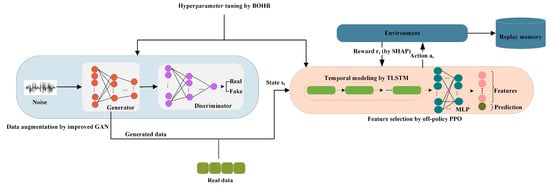
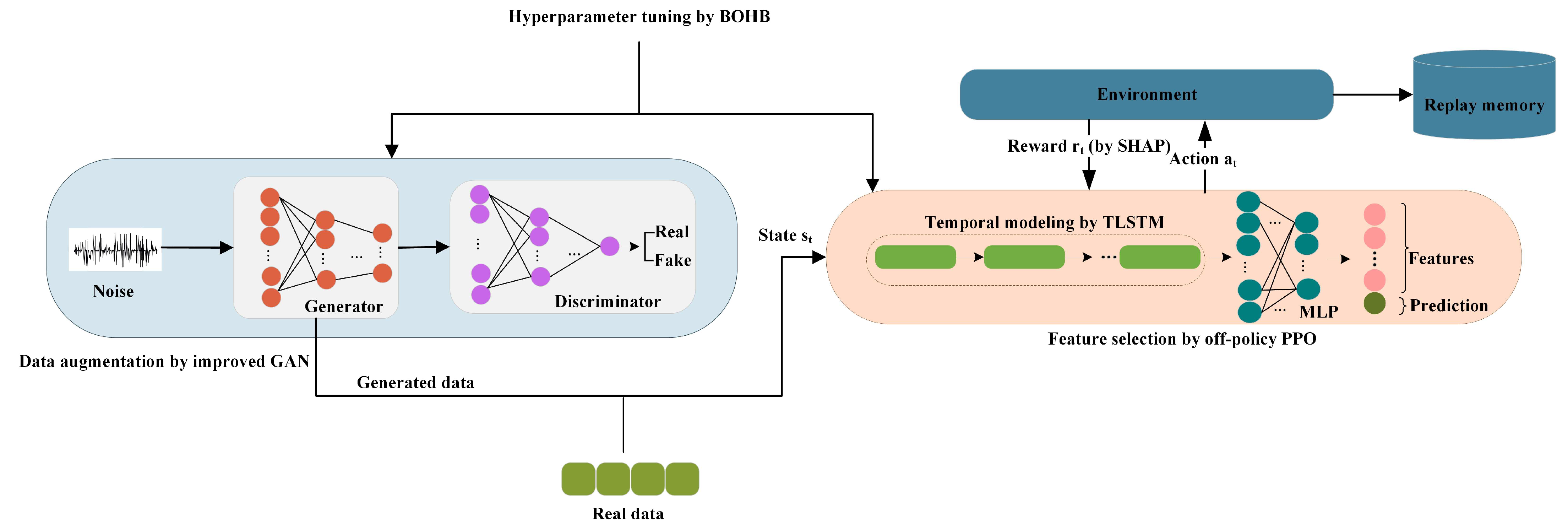
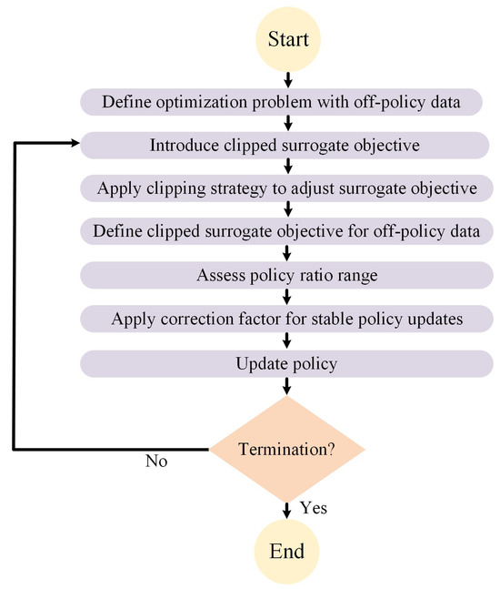
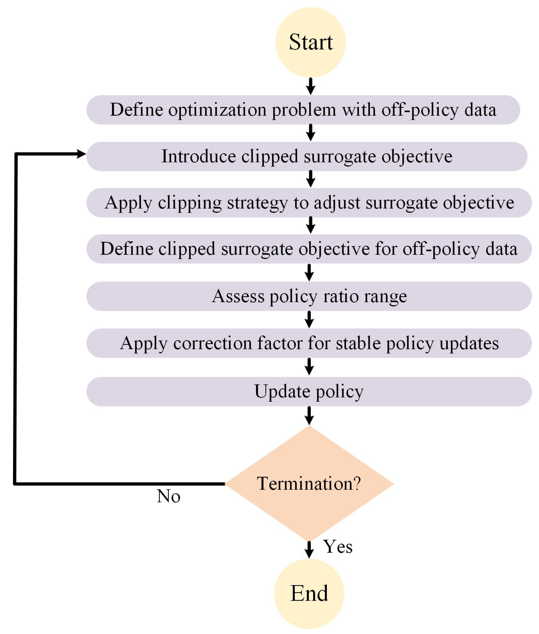
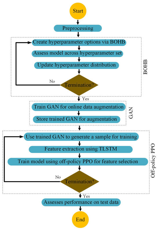
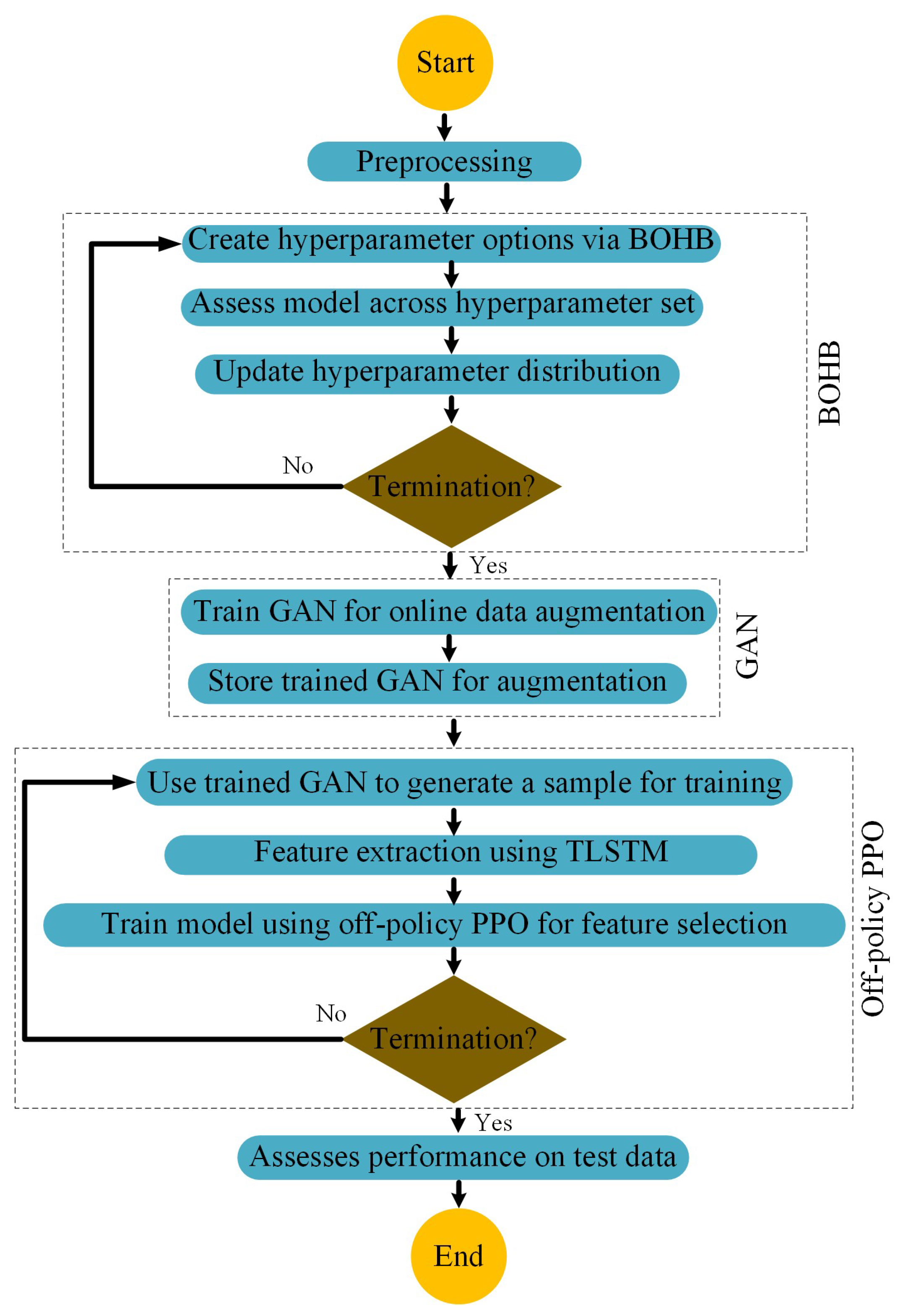
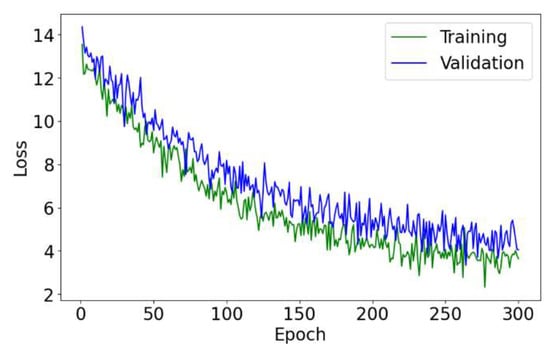
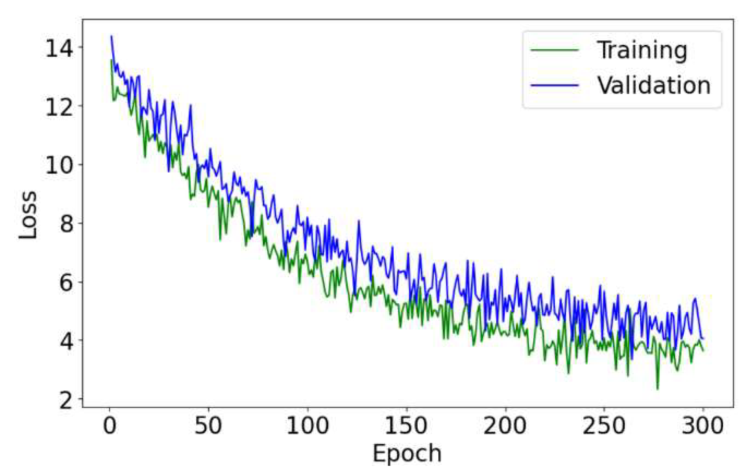
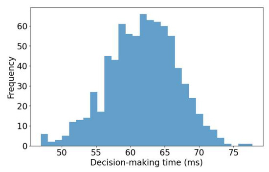
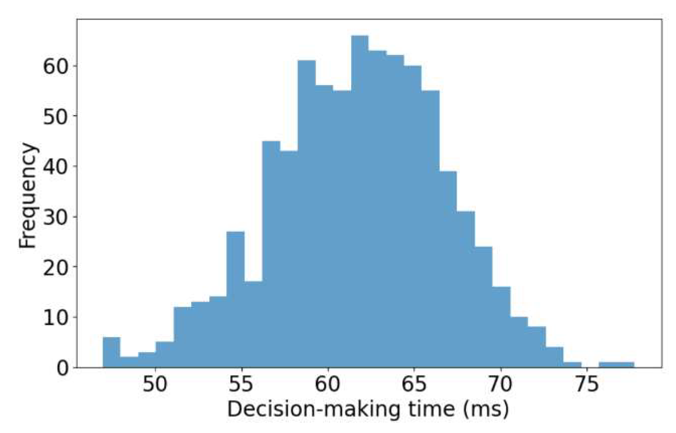
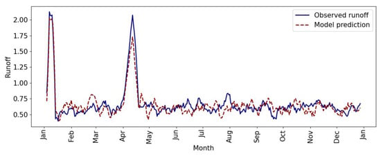
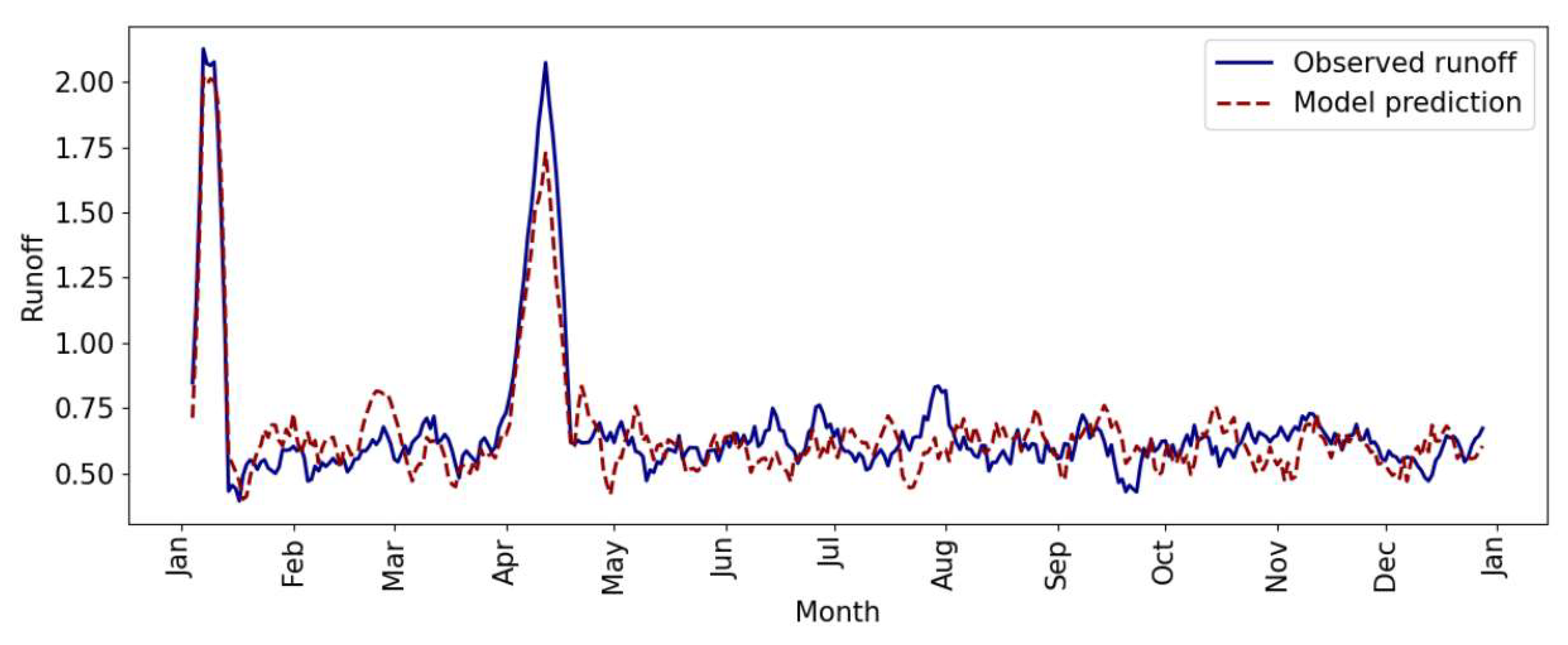
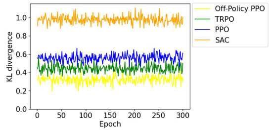
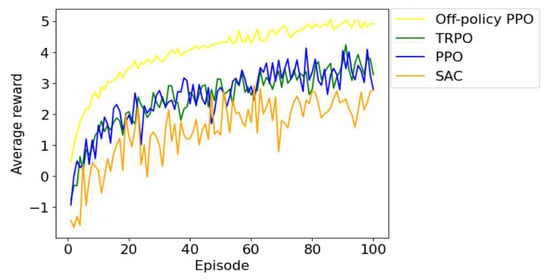
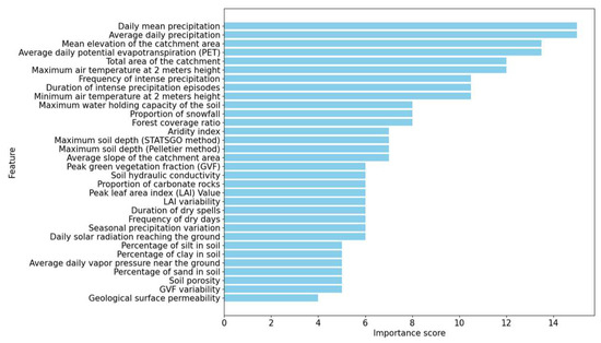
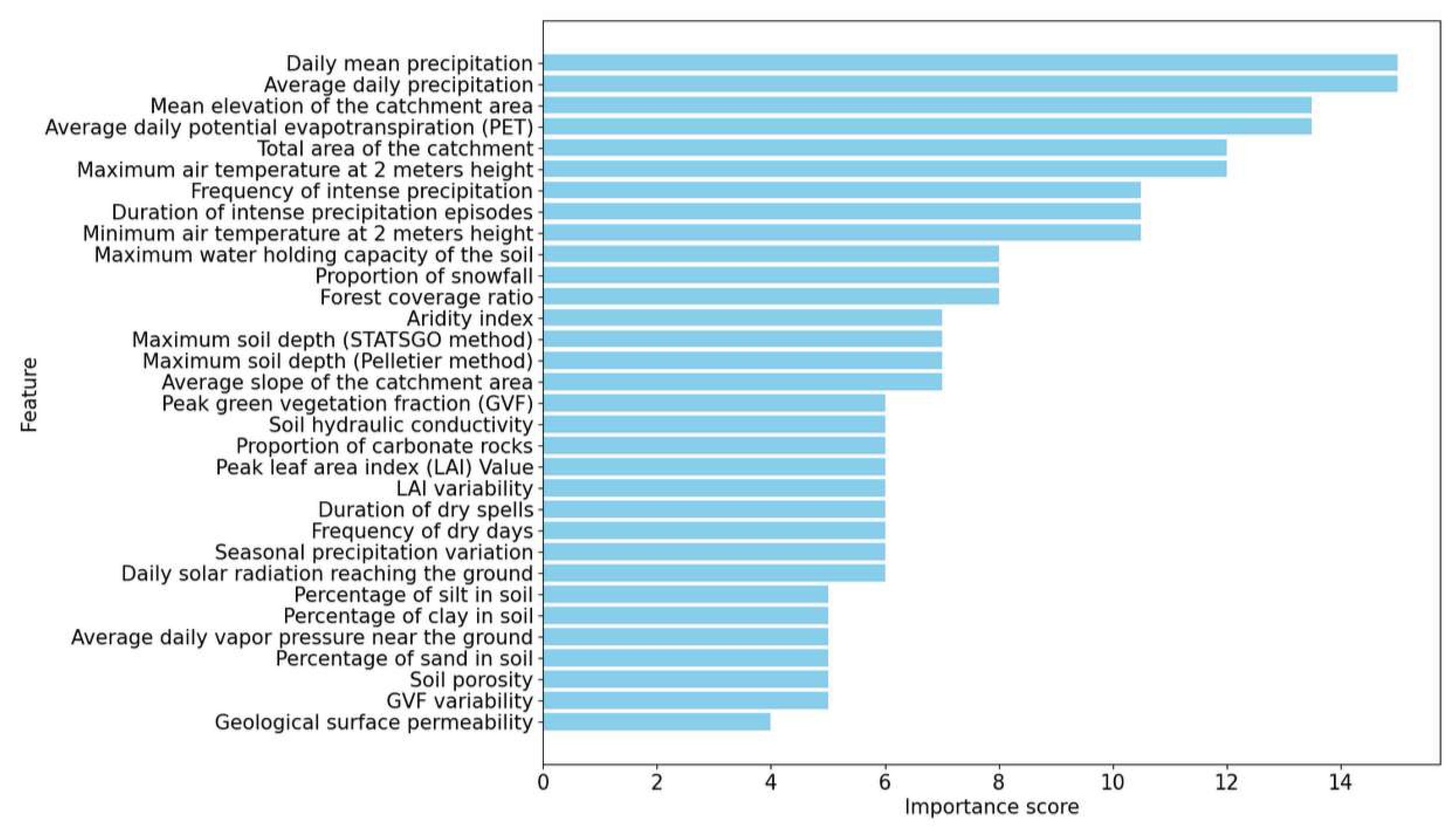
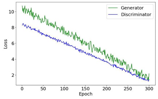
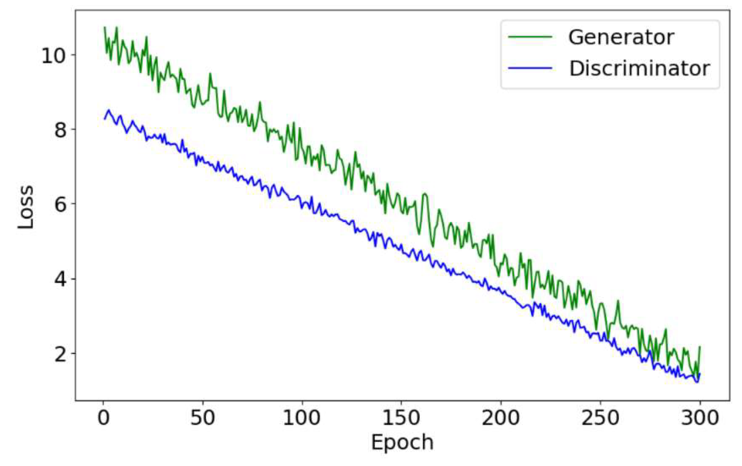
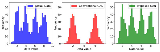
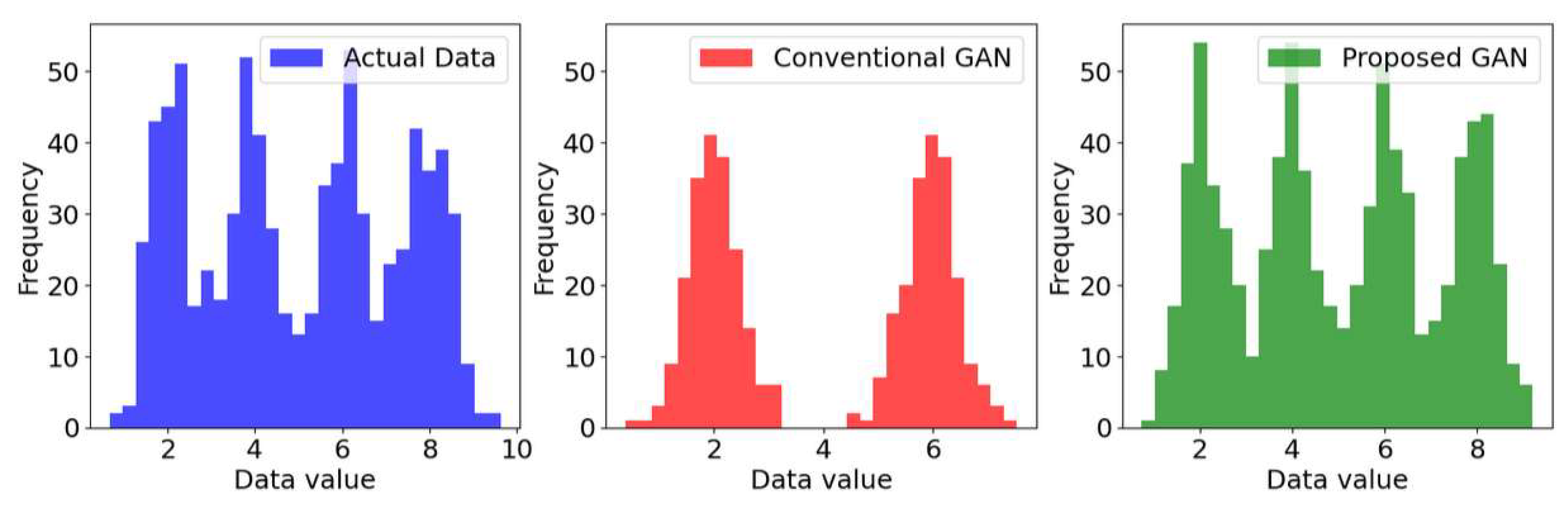
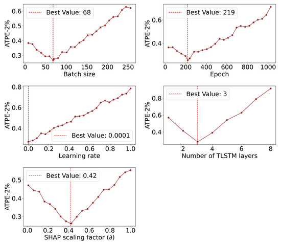
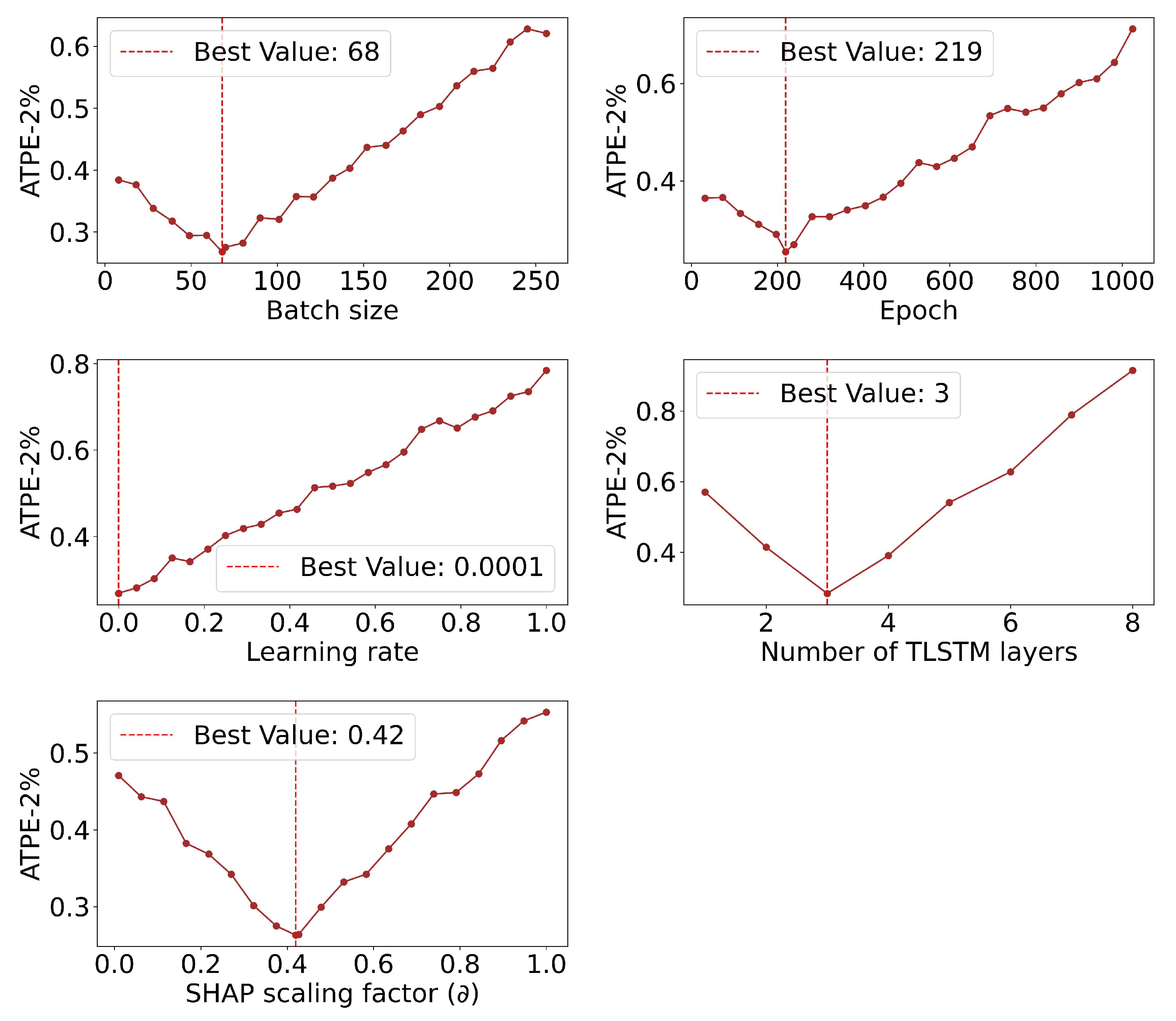

Disclaimer/Publisher’s Note: The statements, opinions and data contained in all publications are solely those of the individual author(s) and contributor(s) and not of MDPI and/or the editor(s). MDPI and/or the editor(s) disclaim responsibility for any injury to people or property resulting from any ideas, methods, instructions or products referred to in the content. |
© 2025 by the authors. Licensee MDPI, Basel, Switzerland. This article is an open access article distributed under the terms and conditions of the Creative Commons Attribution (CC BY) license (https://creativecommons.org/licenses/by/4.0/).