On the Continuity of Efficient Solution Mappings in Portfolio Optimization

Abstract

This paper investigates the stability of a portfolio optimization model. After obtaining explicit analytical expressions for the sets of efficient and weakly efficient portfolios and analyzing their structural characteristics, we developed a corresponding framework for stability analysis. Through this framework, we observed that the stability of the solution set mappings, including outer-semicontinuity, inner-semicontinuity and Lipschitz continuity, is closely related to the ranking of the assets’ expected returns. This understanding enables a shift in stability assessment from traditional numerical simulation towards algebraic verification of asset parameters, potentially offering a more effective approach for stability analysis in this class of models.

1. Introduction

Portfolio optimization constitutes a cornerstone of modern financial theory, profoundly shaping the development of financial markets and the practice of investment decision-making. The portfolio optimization problem aims to select an optimal investment strategy that strikes a balance between maximizing returns and minimizing risks. The seminal work in this field was introduced by Harry Markowitz, who proposed the famous mean-variance model in [1]. Since then, this foundational model has been extensively extended and refined, both computationally and theoretically. For further details, refer to [2,3,4,5,6,7].

Ref. [3] proposed a bi-criteria portfolio optimization model with a new portfolio selection rule, where the objective was to minimize the maximum individual risk. In this model, all the efficient portfolios can be analytically derived, and they are not sensitive with respect to the expectations of investments. Recently, ref. [5] further revisited this bi-criteria portfolio optimization model, and not only provided explicit analytical formulas for all the efficient portfolios, but also explored as a whole the set of all the efficient portfolios and its structure, such as dimensionality and distribution.

Note that the input parameters in most portfolio models are calculated by looking at past data and are inevitably affected by statistical errors. Therefore, one of the main issues in portfolio models that typically needs to be addressed is whether they are stable to small errors in the input parameters. As we know, the mean-variance model has been found that the composition of the optimal portfolio can be very sensitive to estimation errors in the expected returns of the underlying assets, and a small change may lead to a large deviation in practical application (see [8,9] for more details). Kondor et al. [10] studied and compared the sensitivity to estimation error of portfolios optimized under various risk measures, and found that the effect of noise was significant in all the investigated cases. Intuitively, stability requires that small perturbations or small measurement errors of parameters can ensure small changes in the optimal solution or optimal value. From a numerical point of view, it is important to understand the behavior of the solution when the problem is perturbed, which can be used to prove the reliability of the solution. Stability analysis consists of the study of various continuity properties of perturbation maps, including outer and inner semicontinuity, upper and lower semicontinuity, and Lipschitz continuity. We refer to [11,12,13,14] and references therein for more details.

Despite many benefits from the bi-criteria portfolio optimization model in [3], and the set of all efficient portfolios and its structure have been provided in [5], it should be pointed out that the stability analysis of this model has not been explored. In this paper, we will not only provide explicit analytical formulas for the sets of all the efficient and weakly efficient portfolios, but also explore, respectively, the stability analysis of the efficient and weakly efficient solution set mappings with respect to the expected return rates and absolute deviations of assets.

As far as we know, most articles study the stability of models, usually using the following two methods: (1) Established stability analysis results utilizing stability and sensitivity conditions, as well as boundedness and closedness conditions of the objective function and constraint functions; refer to [15,16,17,18]. (2) Utilizing high-performance computing to simulate countless market scenarios and experience-mixed strategies to achieve the stability performance of model; refer to [19,20]. Compared with the first classical stability analysis methods, the main differences in our approach can be summarized in two aspects. On the one hand, the classical stability analysis results are often established by utilizing stability and sensitivity conditions, as well as boundedness and closedness conditions of the objective function and constraint functions. In contrast, we analyze the stability properties based on the crucial fact that the bi-criteria portfolio optimization model we study in this paper allows for analytic expressions of efficient and weakly efficient solutions. The ultimate conclusions indicate that either the outer semicontinuity, inner semicontinuity, or Lipschitz continuity is intrinsically related to the ranking of the expected returns of various assets. This is the most significant difference between the analytical approach adopted in this paper and the classical methods. Simultaneously, this also shows that the stability results we establish cannot be directly derived from the classical results, although our model is specific. On the other hand, the classical stability analysis methods, as far as we know, usually employ inconsistent approaches to characterize the outer and inner semi-continuity and the Lipschitz continuity. However, in this paper, we analyze the aforementioned stability properties from a unified perspective by carrying out analytical expressions of efficient and weakly efficient solution sets.

Many scholars adopt the second classical stability analysis method to study stability. Ref. [20] proposed a portfolio model proposed and using empirical financial data to prove the stability of the model. The contemporary landscape of portfolio optimization is increasingly dominated by data-intensive computational frameworks, such as the generative model approach of [19]. These methods leverage high-performance computing to simulate countless market scenarios and empirically blend strategies to achieve robust performance. While powerful, these approaches are inherently numerical, and their stability is learned from historical data rather than guaranteed by design. Our work is grounded in a specific, analytically solvable bi-criteria model. We establish the stability of the model’s solution set itself with respect to input parameters (such as semi-continuity and Lipschitz continuity) through rigorous mathematical proof. This method provides deterministic theoretical guarantees and reveals the intrinsic relationship between stability and the ranking of assets’ expected returns. Our results therefore serve a dual purpose: they fill a theoretical gap for this specific model and demonstrate how analytical stability results can provide a foundational understanding of model sensitivity. The classical, analytical stability analysis method adopted in this paper forms a valuable contrast and complement to the modern data-driven.

Motivated by the advantage of the bi-criteria portfolio optimization model, we explored as a whole the set of all the efficient portfolios and their structure, such as dimensionality and distribution. Furthermore, we explore, respectively, the stability analysis of the efficient and weakly efficient solution set mappings. The main contributions of this paper are summed up as follows.

• We derived the complete efficient solution set, the weakly efficient solution set of the model, and obtained the relevant properties.
• The stability of the model was explored by studying the outer semi-continuity, inner semi-continuity, continuity and Lipschitz continuity of the effective solution set mapping and weakly effective solution set mapping of this model.
• The primary strength of this paper lies in its novel methodology: leveraging the structure of the analytical solution to prove stability. This approach is feasible because the specific bi-criteria model studied admits a complete characterization, resulting in the efficient solution set being a union of polytopes.
• Classical stability analysis is usually established by utilizing the stability and sensitivity conditions of the objective function and constraint function, as well as the boundedness and closure conditions. This paper analyzes the stability of the model based on the analytical expressions and structures of the effective solution set and weak effective solution set of the model. This is the difference between the analytical method adopted in this article and the classical method.

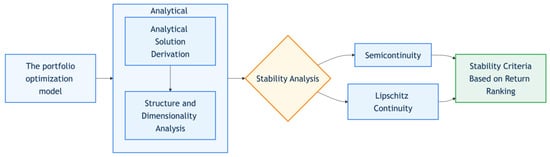
To provide a clear roadmap of the analytical journey undertaken in this study, Figure 1 schematically illustrates the overall research framework and logical flow. This workflow guides the reader through the key stages of our investigation, from foundational model establishment to the final stability conclusions.

Figure 1. Analytical workflow for stability assessment.

The organization of the paper is as follows. In Section 2, we recall some basic definitions and notations. In Section 3, we provide analytic derivations as well as structures for both efficient and weakly efficient solution sets of a bi-criteria portfolio optimization model under a minimax rule. In Section 4, we apply the analytic derivations in Section 3 to establish the outer-semicontinuity, inner-semicontinuity, and Lipschitz continuity for efficient and weakly efficient solution set mappings, respectively. Section 5 presents numerical simulations to verify the theoretical results. Finally, we give some conclusions in Section 6.

2. Preliminaries and Notations

Throughout this paper, all vectors are regarded as column vectors. Let ${\mathbb{R}}^n$ be an n-dimensional Euclidean space, and denote by $x^T$ the transpose of a vector $x\in {\mathbb{R}}^n$. Let $e_j\in {\mathbb{R}}^n$ be the vector with the j-th entry equal to 1 and all others 0, and $e\in {\mathbb{R}}^n$ be the vector all of whose entries are 1. For any $x,y\in {\mathbb{R}}^n$, denote their inner product by $⟨x,y⟩$, the induced distance by $d(x,y)= \parallel x-y\parallel$, and the line segment between them by $[x,y]=\{\lambda x+(1-\lambda )y\mid \lambda \in [0,1\left]\right\}$. Let $\Omega \subset {\mathbb{R}}^n$ be a nonempty set. We denote by $\mathrm{aff}\Omega$, $\mathrm{conv}\Omega$, and $\mathrm{cone}\Omega$ the affine hull, convex hull, and conic hull of $\Omega$, respectively. The distance function associated with $\Omega$ is defined as

$$d(x;\Omega )=inf\{\parallel x-\omega \parallel \mid \omega \in \Omega \},x\in {\mathbb{R}}^n.$$

Given two closed and nonempty subsets $C,D\subset {\mathbb{R}}^n$, the Pompeiu–Hausdorff distance between C and D is denoted by

$$d_{\infty }(C,D)=\underset{x\in {\mathbb{R}}^n}{sup}|d(x;C)-d(x;D)|=max\left\{\underset{x\in D}{sup}d(x;C),\underset{x\in C}{sup}d(x;D)\right\}.$$

Given a nonempty convex subset $Q\subset {\mathbb{R}}^n$, we denote by $\mathrm{ri}Q$ the relative interior of Q. A set $C\subset {\mathbb{R}}^n$ is said to be locally closed at a point $\overline{x}$ (not necessarily in C) if $C\bigcap V$ is closed for some closed neighborhood V of $\overline{x}$.

Next, we recall some standard definitions and properties from variational analysis, which are important for our study in this paper.

Definition 1

([14]). Consider a mapping $S:{\mathbb{R}}^n\rightrightarrows {\mathbb{R}}^m$, a set $X\subset {\mathbb{R}}^n$, and any point $\overline{x}\in X$.

(i) 

S is said to be outer semicontinuous at $\overline{x}$ relative to X if $x^v\in X$, $x^v\to \overline{x}$ and $S\left(x^v\right)\to D$ imply $D\subset S\left(\overline{x}\right)$.

(ii) 

S is said to be inner semicontinuous at $\overline{x}$ relative to X if $x^v\in X$, $x^v\to \overline{x}$ and $S\left(x^v\right)\to D$ imply $D\supset S\left(\overline{x}\right)$.

Definition 2

([14]). A mapping $S:{\mathbb{R}}^n\rightrightarrows {\mathbb{R}}^m$ is said to be Lipschitz continuous on X, a subset of ${\mathbb{R}}^n$, if it is nonempty-closed-valued on X and there exists $\kappa \in {\mathbb{R}}_{+}$, a Lipschitz constant, such that

$$d_{\infty }(S\left(x^{\prime }\right),S\left(x\right))\le \kappa \parallel x^{\prime }-x\parallel ,\forall x,x^{\prime }\in X.$$

or in equivalent geometric form, $S\left(x^{\prime }\right)\subset S\left(x\right)+\kappa |x^{\prime }-x|\mathbb{B},\forall x,x^{\prime }\in X$.

Next, we define the symbol matrix

$$O\left(r\right):={\left[sign(r_i-r_j)\right]}_{n\times n},$$

(1)

where if $r_i-r_j>0$, then $O{\left(r\right)}_{ij}=1$; if $r_i-r_j=0$, then $O{\left(r\right)}_{ij}=0$; if $r_i-r_j<0$, then $O{\left(r\right)}_{ij}=-1$. Suppose that $r_1\le r_2\cdots \le r_n$, there are $2^{n-1}$ different sorting methods. Let $A:=\{r:r_1\le r_2\cdots \le r_n\}$, $\mathcal{O}:=\{O\left(r\right):r_1\le r_2\cdots \le r_n\}$. For $r\in A$, we can uniquely find $O\in \mathcal{O}$ to correspond to it.

In this paper, assume that an investor has initial wealth $M_0=1$, which is to be invested in n possible assets $S_j$, $j=1,\cdots ,n$. Let $R_j$ be the return rate of the asset $S_j$, which is a random variable. Let $x_j$ be the allocation for investment to $S_j$ and $x_j\ge 0$, $j=1,\cdots ,n$. Note that we are concerned with the situation where short-selling is not allowed. Let $\mathrm{E}\left(R\right)$ denote the mathematical expectation of a random variable R. Define

$$r_j:=\mathrm{E}\left(R_j\right),q_j:=\mathrm{E}\left(\right|R_j-r_j\left|\right),$$

that is, $r_j$ and $q_j$ denote the expected return rate of the asset $S_j$ and the expected absolute deviation of $R_j$ from its mean, $j=1,\cdots ,n$, respectively. For any given feasible portfolio x, its expected return is given by

$$\pi \left(x\right):=\mathrm{E}\left({\displaystyle \sum _{j=1}^n}{R}_j{x}_j\right)={\displaystyle \sum _{j=1}^n}\mathrm{E}\left(R_j\right)x_j={\displaystyle \sum _{j=1}^n}{r}_j{x}_j.$$

The $l_{\infty }$ risk function is defined as

$$\omega \left(x\right):=\underset{1\le j\le n}{max}{q}_j{x}_j.$$

The portfolio optimization problem can be formulated as a bi-criteria linear program:

$$\mathrm{minimize}(\underset{1\le j\le n}{max}{q}_j{x}_j,-{\displaystyle \sum _{j=1}^n}{r}_j{x}_j)$$

$$\mathrm{s}\mathrm{u}\mathrm{b}\mathrm{j}\mathrm{e}\mathrm{c}\mathrm{t} \mathrm{t}\mathrm{o}{\displaystyle \sum _{j=1}^n}{x}_j=1,$$

(2)

$$x_j\ge 0,j=1,2,\cdots ,n.$$

Recall that a feasible portfolio x is said to be efficient if there exists no feasible portfolio $x^{\prime }$ such that $\omega \left(x^{\prime }\right)\le \omega \left(x\right),\pi \left(x^{\prime }\right)\ge \pi \left(x\right)$, and at least one of the inequalities holds strictly.

A feasible portfolio x is said to be weakly efficient if there exists no feasible portfolio $x^{\prime }$ such that $\omega \left(x^{\prime }\right)<\omega \left(x\right),\pi \left(x^{\prime }\right)>\pi \left(x\right)$. Accordingly, the function value $\left(\omega \right(x),\pi (x\left)\right)$ is said to be an efficient (resp. weakly efficient) point in the risk–return (i.e., $\omega -\pi$) plane if x is efficient (resp. weakly efficient).

Let $S:{\mathbb{R}}^n\times {\mathbb{R}}_{++}^n\rightrightarrows {\mathbb{R}}^n$ and $S^w:{\mathbb{R}}^n\times {\mathbb{R}}_{++}^n\rightrightarrows {\mathbb{R}}^n$ be the efficient solution set mapping and the weakly efficient solution set mapping of the bi-criteria linear program (2), respectively. Given $(r,q)\in {\mathbb{R}}^n\times {\mathbb{R}}_{++}^n$, it is clear that $S(r,q)$ (resp. $S^w(r,q)$) is the set of all efficient (resp. weakly efficient) portfolios of (2) and $S(r,q)\subset S^w(r,q)$.

Remark 1.

The following assumptions are made throughout the rest of this paper:

(A1) 

All assets are risky (i.e., $q_i>0$ for all i).

(A2) 

The expected return rate of all assets is not exactly the same (i.e., there exist some j and k such that $r_j\ne r_k$).

(A3) 

The assets are ranked based on their expected return rate (such as $r_1\le r_2\le \cdots \le r_n$).

These assumptions are crucial for our analysis. (A1) establishes that all assets are risky, thereby excluding risk-free assets. (A2) states that assets have differing expected returns, a necessary precondition for subsequent analysis such as ranking and optimization. (A3) is indispensable for the subsequent proofs in Section 3 and Section 4. From a financial perspective, the analysis in this paper relies on specific modeling choices, such as the prohibition of short-selling and the adoption of absolute deviation as a risk measure. While this setup is key to obtaining geometric results, it nevertheless limits the model’s direct applicability to markets where short-selling is permitted or where alternative risk measures like variance are more relevant.

3. Analytic Derivation of Efficient/Weakly Efficient Portfolios

The main purpose of this section is to present an analytic derivation of $S(r,q)$ ($S^w(r,q)$). To analytically characterize the efficient and weakly efficient sets for (2), we adopt a three-stage research strategy. First, we transform the problem into a single-objective optimization problem (5) through parametric scalarization, which allows the efficient set $S(r,q)$ to be expressed as the union of all optimal solution sets $E\left(\lambda \right)$ for $\lambda >0$. Second, under the assumption of ordered returns, we explicitly derive the polytopic structure of $E\left(\lambda \right)$, thereby providing a complete characterization of $S(r,q)$ as a union of connected polytopes. Finally, we construct the weakly efficient set $S^w(r,q)$ by augmenting the efficient set with the optimal solutions from two extreme cases (namely, the optimization problems (22) and (23), where one of the two objective functions is entirely neglected).

To begin with, we introduce some notations that are important for our analysis. Throughout this paper, let $I:=\{1,2,\cdots ,n\}$. Take arbitrarily $r\in {\mathbb{R}}^n$ and $k\in I$, let $r_{max}:=max\{r_j\mid j\in I\}$, $r_{min}:=min\{r_j\mid j\in I\}$, $I^{+}(r,k):=\{j\in I\mid r_j>r_k\}$, $I^0(r,k):=\{j\in I\mid r_j=r_k\}$, $I^{-}(r,k):=\{j\in I\mid r_j<r_k\}$, $I_{max}^0\left(r\right):=\{j\in I\mid r_j=r_{max}\}$.

Simultaneously, we define the function $g:\mathbb{R}\to \mathbb{R}$ by $g\left(t\right):={\sum }_{j=1}^n{\displaystyle \frac{{(r_j-t)}_{+}}{q_j}}$, and the function $h:\mathbb{R}\to \mathbb{R}$ by $h\left(t\right)=-g_{-}^{\prime }\left(t\right)$. In the case of $r_1\le r_2\le \cdots \le r_n$ and $q\in {\mathbb{R}}_{++}^n$, we set

$$x^{0,1}:={\left({\displaystyle \frac{1}{q_1}},{\displaystyle \frac{1}{q_2}},\cdots ,{\displaystyle \frac{1}{q_n}}\right)}^T/{\displaystyle \sum _{i=1}^n}{\displaystyle \frac{1}{q_i}},$$

(3)

and for each $2\le k\le n$, define $x^{k-1,k}$ by

$$\begin{array}{c}\hfill \begin{array}{c}\hfill x^{k-1,k}=\left\{\begin{array}{cc}{\displaystyle \frac{1}{q_j}}/{\displaystyle {\sum }_{i=k}^n}{\displaystyle \frac{1}{q_i}},\hfill & ifk\le j\le n,\hfill \\ 0,\hfill & if1\le j\le k-1.\hfill \end{array}\right.\end{array}\end{array}$$

(4)

The following lemma, which is useful for our analytic derivation, follows readily from the definitions of g and h.

Lemma 1.

In the case of $r_1\le r_2\le \cdots \le r_n$. The following properties of g and h hold:

(a) 

h is a decreasing upper semi-continuous step function, and $h\left(t\right)>0$ for all $t\le r_n$. Explicitly, we have

$$\begin{array}{c}\hfill \begin{array}{c}\hfill h\left(t\right)=\left\{\begin{array}{cc}{\displaystyle {\sum }_{j=1}^n}{\displaystyle \frac{1}{q_j}},\hfill & ift\le r_1,\hfill \\ {\displaystyle {\sum }_{j=k}^n}{\displaystyle \frac{1}{q_j}},\hfill & if{r}_{k-1}<t\le r_k,\hfill \\ 0,\hfill & ift>r_n.\hfill \end{array}\right.\end{array}\end{array}$$

(b) 

g is a continuous piecewise linear convex function. Explicitly, we have

$$\begin{array}{c}\hfill \begin{array}{c}\hfill g\left(t\right)=\left\{\begin{array}{cc}g\left(r_1\right)+(r_1-t)h\left(r_1\right),\hfill & ift\le r_1,\hfill \\ g\left(r_k\right)+(r_k-t)h\left(r_k\right),\hfill & if{r}_{k-1}<t\le r_k,\hfill \\ 0,\hfill & ift>r_n.\hfill \end{array}\right.\end{array}\end{array}$$

(c) 

$g\left(t\right)$ is strictly decreasing on $(-\infty ,r_n]$, and ${min}_{t\in \mathbb{R}}g\left(t\right)=0$. Further, $g\left(r_n\right)=0$.

The following lemma, which is a direct consequence of (ref. [14], Exercise 8.31), plays an important role in deriving optimality conditions for (2).

Lemma 2.

Let $x\in {\mathbb{R}}^n$ with $x\ne 0$. Then $v\in \partial \omega \left(x\right)$ if and only if $x_j={\displaystyle \frac{\omega \left(x\right)}{q_j}},if{v}_j>0$ and ${\sum }_{v_j>0}{\displaystyle \frac{v_j}{q_j}}=1.$

Analytic Derivation of Efficient Portfolios

To seek $S(r,q)$ for the bi-criteria piecewise linear convex program (2), we can convert (2) into a parametric optimization problem

$$\mathrm{minimize}\lambda \omega \left(x\right)-\pi \left(x\right)$$

$$\mathrm{subject} \mathrm{to}{\displaystyle \sum _{j=1}^n}{x}_j=1,$$

(5)

$$x_j\ge 0,j=1,2,\cdots ,n,$$

where $\lambda >0$. The feasible region of (5) is

$$\mathcal{F}=\{x=(x_1,x_2,···,x_n)|{\displaystyle \sum _{j=1}^n}{x}_j=1,x_j\ge 0,j=1,2,\cdots ,n\}.$$

Note that the function $\lambda \omega \left(x\right)-\pi \left(x\right)$ is a continuous function and the feasible region $\mathcal{F}$ is a compact set. Thus, the parametric optimization problem (5) has a nonempty optimal solution set $E\left(\lambda \right)$ for all $\lambda >0$. In addition, since (2) is a bi-criteria piecewise linear convex program and $\mathcal{F}$ is compact, it follows from (ref. [21], Theorem 3.4) that x is an efficient portfolio if and only if there is some $\lambda >0$ such that $x\in E\left(\lambda \right)$. This entails that

$$S(r,q)=\bigcup _{\lambda >0}E\left(\lambda \right).$$

(6)

Now we are ready for providing an analytic derivation of $E\left(\lambda \right)$, i.e., the optimal solution set of the parametric optimization problem (5), when r in particular satisfies $r_1\le r_2\le \cdots \le r_n$.

Theorem 1.

Suppose that $r_1\le r_2\le \cdots \le r_n$ and $\lambda >0$. Then, $x\in E\left(\lambda \right)$ if and only if each component $x_j$ can be written as

$$x_j={\displaystyle \frac{{\theta }_j}{q_j}}/\left({\displaystyle \sum _{i=1}^n}{\displaystyle \frac{{\theta }_i}{q_i}}\right),$$

(7)

where $\theta \in {\mathbb{R}}^n$ is any vector satisfying

(a) 

In the case of $g\left(r_1\right)<\lambda <+\infty$: if $r_j\ge r_1$, then ${\theta }_j=1$. i.e., $E\left(\lambda \right)=\left\{x^{0,1}\right\}$ in this case;

(b) 

In the case of $g\left(r_k\right)<\lambda <g\left(r_{k-1}\right)$ for some $k\in \{2,\cdots ,n\}$:

$$\begin{array}{c}\hfill \begin{array}{c}\hfill {\theta }_j=\left\{\begin{array}{cc}1,\hfill & if{r}_j\ge r_k,\hfill \\ 0,\hfill & if{r}_j\le r_{k-1},\hfill \end{array}\right.\end{array}\end{array}$$

i.e., $E\left(\lambda \right)=\left\{x^{k-1,k}\right\}$ in this case;

(c) 

In the case of $\lambda =g\left(r_k\right)$ with $r_k<r_n$: $0\le {\theta }_j\le 1,if{r}_j=r_k$ and

$$\begin{array}{c}\hfill \begin{array}{c}\hfill {\theta }_j=\left\{\begin{array}{cc}1,\hfill & if{r}_j>r_k,\hfill \\ 0,\hfill & if{r}_j<r_k.\hfill \end{array}\right.\end{array}\end{array}$$

Proof. 

In view of Lemma 1(c), we have $0=g\left(r_n\right)\le g\left(r_{n-1}\right)\le \cdots \le g\left(r_2\right)\le g\left(r_1\right)<+\infty$, and $g\left(r_k\right)<g\left(r_{k-1}\right)$ whenever $r_{k-1}<r_k\le r_n$. To fully characterize the optimal solution set $E\left(\lambda \right)$ of the parametric optimization problem (4) for all $\lambda >0$, we only need to consider cases (a)–(c).

According to the optimality condition for convex optimization (ref. [14], Theorem 8.15), x is an optimal solution to (4) if and only if there exists some $\tau \in \mathbb{R}$ such that

$${\displaystyle \sum _{j=1}^n}{x}_j=1,$$

(8)

$$x_j\ge 0,j=1,2,\cdots ,n,$$

(9)

and

$$r-\tau e\in \lambda \partial \omega \left(x\right).$$

(10)

It follows from (8) and (9) that there exists $j\in I=\{1,2,\cdots ,n\}$ such that $x_j>0$, and then $\omega \left(x\right)>0$. Depending on the value of $\tau$, we can divide I into three distinct subindex sets as follows: $I^{+}:=\{j\in I\mid r_j>\tau \},I^0:=\{j\in I\mid r_j=\tau \},I^{-}:=\{j\in I\mid r_j<\tau \}$. By Lemma 2, (10) holds if and only if

$$x_j={\displaystyle \frac{\omega \left(x\right)}{q_j}},j\in I^{+}and\sum _{j\in I^{+}}(r_j-\tau ){\displaystyle \frac{1}{q_j}}=\lambda .$$

(11)

By employing the function g, the latter equation shows

$$g\left(\tau \right)=\lambda .$$

(12)

It follows from Lemma 1 and (12) that $\lambda =g\left(\tau \right)>0$ if and only if $\tau <r_n$. By the definition of $\omega \left(x\right)$, we have

$$0\le x_j\le {\displaystyle \frac{\omega \left(x\right)}{q_j}},\forall j\in I^0.$$

(13)

In view of (11), we deduce that (8) holds if and only if there are some ${\theta }_j\in [0,1]$ with $j\in I^0$ such that

$$x_j={\displaystyle \frac{{\theta }_j\omega \left(x\right)}{q_j}},\forall j\in I^0$$

(14)

and

$$\sum _{j\in I^{+}}{\displaystyle \frac{1}{q_j}}+\sum _{j\in I^0}{\displaystyle \frac{{\theta }_j}{q_j}}={\displaystyle \frac{1}{\omega \left(x\right)}}.$$

(15)

By Lemma 1(c), we can conclude that the Equation (12) has a (unique) solution in $\tau \in (-\infty ,r_n)$. It remains to show (a)–(c) by first identifying the unique $\tau \in (-\infty ,r_n)$ satifying (12), and then using the relations (11) and (13)–(15) to describe components $x_j$ of each $x\in E\left(\lambda \right)$ as follows:

$$x_j={\displaystyle \frac{{\theta }_j\omega \left(x\right)}{q_j}}={\displaystyle \frac{{\theta }_j}{q_j}}/\left(\sum _{j\in I^{+}}{\displaystyle \frac{1}{q_j}}+\sum _{j\in I^0}{\displaystyle \frac{{\theta }_j}{q_j}}\right)={\displaystyle \frac{{\theta }_j}{q_j}}/\left({\displaystyle \sum _{i=1}^n}{\displaystyle \frac{{\theta }_i}{q_i}}\right),$$

where $\theta \in {\mathbb{R}}^n$ is any vector satisfying

$$\begin{array}{c}\hfill \begin{array}{c}\hfill {\theta }_j=\left\{\begin{array}{cc}1,\hfill & j\in I^{+},\hfill \\ 0,\hfill & j\in I^{-},\hfill \end{array}\right.\mathrm{and}0\le {\theta }_j\le 1,j\in I^0,\end{array}\end{array}$$

(16)

and

$${\displaystyle \sum _{i=1}^n}{\displaystyle \frac{{\theta }_i}{q_i}}>0.$$

(17)

Now, we are at the position to determine the value of the unique $\tau \in (-\infty ,r_n)$, in an analytical way, via the piecewise linear Equation (12) for all particular cases (a)–(c).

In case (a), we have $\lambda =g\left(\tau \right)>g\left(r_1\right)$, and then $\tau <r_1$. By Lemma 1$\left(b\right)$, we get $\lambda =g\left(r_1\right)+h\left(r_1\right)(r_1-\tau )$, which implies $\tau =r_1+{\displaystyle \frac{g\left(r_1\right)-\lambda }{h\left(r_1\right)}}$. This shows that $I^{+}=\{1,2,\cdots ,n\}$, $I^{-}=I^0=\varnothing$ and ${\sum }_{i=1}^n{\displaystyle \frac{{\theta }_i}{q_i}}={\sum }_{i=1}^n{\displaystyle \frac{1}{q_i}}>0$. Thus, (17) holds for the unique $\theta$ satisfying (16).

In case (b), we have $g\left(r_k\right)<\lambda =g\left(\tau \right)<g\left(r_{k-1}\right)$, $k=2,3,\cdots ,n$ and hence $r_{k-1}<\tau <r_k$. By Lemma 1(b), we get $\lambda =g\left(r_k\right)+h\left(r_k\right)(r_k-\tau )$, which implies $\tau =r_k+{\displaystyle \frac{g\left(r_k\right)-\lambda }{h\left(r_k\right)}}$. This shows that that $I^{+}=\{j\in I|r_j\ge r_k\}$, $I^{-}=\{j\in I|r_j\le r_{k-1}\}$, $I^0=\varnothing$ and ${\sum }_{i=1}^n{\displaystyle \frac{{\theta }_i}{q_i}}={\sum }_{i=k}^n{\displaystyle \frac{1}{q_i}}>0$. Thus, (17) holds for the unique $\theta$ satisfying (16).

In case (c), we have $g\left(\tau \right)=\lambda =g\left(r_k\right)$ and hence $\tau =r_k<r_n$. This shows that $I^{+}=\{j\in I|r_j>r_k\}$, $I^{-}=\{j\in I|r_j<r_k\}$, $I^0=\{j\in I|r_j=r_k\}$ and ${\sum }_{i=1}^n{\displaystyle \frac{{\theta }_i}{q_i}}={\sum }_{i\in I^{+}}{\displaystyle \frac{1}{q_i}}+{\sum }_{i\in I^0}{\displaystyle \frac{{\theta }_i}{q_i}}>0$. Thus, (17) holds for all $\theta$ satisfying (16). This completes the proof. □

Theorem 2.

Suppose that $r_1\le r_2\le \cdots \le r_n$ and $r_k<r_n$ for some $k\in I$. Let

$$\Theta =\{\theta \in {\mathbb{R}}^n\mid {\theta }_j=1,\forall j\in I^{+}(r,k);0\le {\theta }_j\le 1,\forall j\in I^0(r,k);{\theta }_j=0,\forall j\in I^{-}(r,k)\}.$$

Then, the following statements on the optimal solution set $E\left(\lambda \right)$ to the parametric optimization problem (4) for $\lambda =g\left(r_k\right)$ are true:

(i) 

$x\in E\left(\lambda \right)$ if and only if $\pi \left(x\right)=g\left(r_k\right)\omega \left(x\right)+r_k$, $⟨e,x⟩=1$ and $x_j\ge 0$ for all $j\in I$.

(ii) 

$E\left(\lambda \right)$ is the solution set of the linear system

$$\begin{array}{c}\hfill \begin{array}{c}\hfill \left\{\begin{array}{cc}{q}_j{x}_j={\displaystyle \frac{\pi \left(x\right)-r_k}{g\left(r_k\right)}},\hfill & j\in I^{+}(r,k),\hfill \\ x_j=0,\hfill & j\in I^{-}(r,k),\hfill \\ q_j{x}_j\le {\displaystyle \frac{\pi \left(x\right)-r_k}{g\left(r_k\right)}},\hfill & j\in I^0(r,k),\hfill \\ -x_j\le 0,\hfill & j\in I^0(r,k),\hfill \\ ⟨e,x⟩=1.\hfill \end{array}\right.\end{array}\end{array}$$

(18)

(iii) 

$E\left(\lambda \right)$ is a polytope. Moreover, x is a vertex of $E\left(\lambda \right)$ if and only if

$$x_j={\displaystyle \frac{{\theta }_j}{q_j}}/\left({\displaystyle \sum _{i=1}^n}{\displaystyle \frac{{\theta }_i}{q_i}}\right),$$

where $\theta \in \Theta$ is any vector satisfying ${\theta }_j\in \{0,1\}$ for all $j\in I^0(r,k)$, entailing that the number of vertices of $E\left(\lambda \right)$ is $2^{|I^0(r,k)|}$. Furthermore, let ${\Theta }_0=\{\theta \in \Theta \mid {\theta }_j\in \{0,1\},\forall j\in I^0(r,k)\}$ and let $x\left(\hat{\theta }\right),x\left(\tilde{\theta }\right)$ with $\hat{\theta },\tilde{\theta }\in {\Theta }_0$ be two vertices of $E\left(\lambda \right)$. Then the closed line segment joining $x\left(\hat{\theta }\right)$ and $x\left(\tilde{\theta }\right)$, denoted by $[x\left(\hat{\theta }\right),x\left(\tilde{\theta }\right)]$, is an edge of $E\left(\lambda \right)$ if and only if there exists $j_{\mathcal{l}}\in I^0(r,k)$ such that ${\hat{\theta }}_j={\tilde{\theta }}_j$ for $j\in I\setminus \left\{j_{\mathcal{l}}\right\}$ and ${\hat{\theta }}_{j_{\mathcal{l}}}+{\tilde{\theta }}_{j_{\mathcal{l}}}=1$. In particular, when $I^0(r,k)=\left\{k\right\}$, $E\left(\lambda \right)=[x^{k-1,k},x^{k,k+1}]$.

(iv) 

The dimension of $E\left(\lambda \right)$ is $|I^0(r,k)|$.

Proof. 

For simplicity, we denote by $\xi \left(k\right)=min{I}^0(r,k)$ and $\eta \left(k\right)=max{I}^0(r,k)$, and denote by $x\left(\theta \right)$ the vector whose components are in the form of (7). According to Theorem 1, $x\in E\left(\lambda \right)$ if and only if $x=x\left(\theta \right)$ for some $\theta \in \Theta$ in the case of $r_k<r_n$. Let $\tilde{x}=x\left(\theta \right)$ with $\theta \in \Theta$ satisfying ${\theta }_j=1$ for all $j\in I^0(r,k)$. Then we have $\tilde{x}\in E\left(\lambda \right)$ and $\tilde{x}=x^{\xi \left(k\right)-1,\xi \left(k\right)}$. By definition and Lemma 1(a), we have $\omega \left(\tilde{x}\right)={\left({\sum }_{j=\xi \left(k\right)}^n{\displaystyle \frac{1}{q_j}}\right)}^{-1}={\displaystyle \frac{1}{h\left(r_k\right)}}$ and $\pi \left(\tilde{x}\right)={\displaystyle \frac{1}{h\left(r_k\right)}}{\sum }_{j=\xi \left(k\right)}^n{\displaystyle \frac{r_j}{q_j}}={\displaystyle \frac{1}{h\left(r_k\right)}}{\sum }_{j=\xi \left(k\right)}^n{\displaystyle \frac{r_j-r_k}{q_j}}+r_k=\omega \left(\tilde{x}\right)g\left(r_k\right)+r_k$. Together with $\lambda =g\left(r_k\right)$, it follows $\lambda \omega \left(\tilde{x}\right)-\pi \left(\tilde{x}\right)=-r_k$, which shows that the optimal value of (4) is $-r_k$. Therefore, $x\in E\left(\lambda \right)$ if and only if $⟨e,x⟩=1$, $x_j\ge 0$, $j\in I$ and $\lambda \omega \left(x\right)-\pi \left(x\right)=-r_k$, i.e., statement (i) is true. By statement (i), Theorem 1 and the definition of $\omega$, we can show that statement (ii) is also true, implying that $E\left(\lambda \right)$ is a convex polyhedron.

To show statement (iii), since the feasible region $\mathcal{F}$ of (5) is a compact set and $E\left(\lambda \right)\subset \mathcal{F}$, it follows that $E\left(\lambda \right)$ is a bounded convex polyhedron, i.e., $E\left(\lambda \right)$ is a polytope. Let $x\in E\left(\lambda \right)$, or equivalently, $x=x\left(\theta \right)$ for some $\theta \in \Theta$. From statements (i–ii), it follows that $x\left(\theta \right)$ is a solution to the following system of equations:

$$\begin{array}{c}\hfill \begin{array}{c}\hfill \left\{\begin{array}{cc}{q}_j{x}_j={\displaystyle \frac{\pi \left(x\right)-r\left(k\right)}{g\left(r_k\right)}},\hfill & j\in I^{+}(r,k),\hfill \\ x_j=0,\hfill & j\in I^{-}(r,k),\hfill \\ q_j{x}_j={\displaystyle \frac{\pi \left(x\right)-r\left(k\right)}{g\left(r_k\right)}},\hfill & j\in I^{0+}(r,k),\hfill \\ x_j=0,\hfill & j\in I^{0-}(r,k),\hfill \\ ⟨e,x⟩=1,\hfill \end{array}\right.\end{array}\end{array}$$

(19)

where $I^{0+}(r,k):=\{j\in I^0(r,k)\mid {\theta }_j=1\},I^{0-}(r,k):=\{j\in I^0(r,k)\mid {\theta }_j=0\}$.

In the case of ${\theta }_j\in \{0,1\}$ for all $j\in I^0(r,k)$, it follows from statements (i–ii) that each $x\left(\tilde{\theta }\right)$ with $\tilde{\theta }\in \Theta \setminus \left\{\theta \right\}$ violates at least one equation in (19), implying that $x\left(\theta \right)$ is the unique solution to the system of linear Equation (19) and hence a vertex of $E\left(\lambda \right)$. While in the case $0<{\theta }_{j_0}<1$ for some $j_0\in I^0(r,k)$, the vector $x\left(\tilde{\theta }\right)$ with ${\tilde{\theta }}_j={\theta }_j$ for all $j\in I^0(r,k)/\left\{j_0\right\}$ and ${\tilde{\theta }}_{j0}={\displaystyle \frac{1}{2}}{\theta }_{j_0}$ is another distinct solution to the system of linear Equation (19), implying that $x\left(\theta \right)$ is not a vertex of $E\left(\lambda \right)$. So, x is a vertex of $E\left(\lambda \right)$ if and only if $x=x\left(\theta \right)$ for any $\theta \in \Theta$ satisfying ${\theta }_j\in \{0,1\}$ for all $j\in I^0(r,k)$. The number of vertices of $E\left(\lambda \right)$ is $2^{|I^0(r,k)|}$, and in particular, $x^{\xi \left(k\right)-1,\xi \left(k\right)}$ is a vertex of $E\left(\lambda \right)$.

Let $x\left(\hat{\theta }\right),x\left(\tilde{\theta }\right)$ with $\hat{\theta },\tilde{\theta }\in {\Theta }_0$ be two vertices of $E\left(\lambda \right)$. On the one hand, assume that there exists $j_{\mathcal{l}}\in I^0(r,k)$ such that ${\hat{\theta }}_j={\tilde{\theta }}_j$ for $j\in I\setminus \left\{j_{\mathcal{l}}\right\}$ and ${\hat{\theta }}_{j_{\mathcal{l}}}+{\tilde{\theta }}_{j_{\mathcal{l}}}=1$. From statements (i–ii), it follows that $[x\left(\hat{\theta }\right),x\left(\tilde{\theta }\right)]$ is contained in the solution set to the following system of equations:

$$\begin{array}{c}\hfill \begin{array}{c}\hfill \left\{\begin{array}{cc}{q}_j{x}_j={\displaystyle \frac{\pi \left(x\right)-r_k}{g\left(r_k\right)}},\hfill & j\in I^{+}(r,k),\hfill \\ x_j=0,\hfill & j\in I^{-}(r,k),\hfill \\ x_j={\displaystyle \frac{\pi \left(x\right)-r_k}{q_{j}g\left(r_k\right)}}\hfill & j\in I^{0+}(r,k)\setminus \left\{j_{\mathcal{l}}\right\},\hfill \\ x_j=0,\hfill & j\in I^{0-}(r,k)\setminus \left\{j_{\mathcal{l}}\right\},\hfill \\ ⟨e,x⟩=1.\hfill \end{array}\right.\end{array}\end{array}$$

(20)

where $I^{0+}(r,k):=\{j\in I^0(r,k)\mid {\hat{\theta }}_j=1\},I^{0-}(r,k):=\{j\in I^0(r,k)\mid {\hat{\theta }}_j=0\}$.

Obviously, the solution to the system of linear Equation (20) is not unique. Note that the solution to the system (19) is unique. Thus, we can conclude from (ref. [12], Theorem 2.3.3) that $[x\left(\hat{\theta }\right),x\left(\tilde{\theta }\right)]$ is a face of $E\left(\lambda \right)$ and the dimension of $[x\left(\hat{\theta }\right),x\left(\tilde{\theta }\right)]$ is equal to one, that is, $[x\left(\hat{\theta }\right),x\left(\tilde{\theta }\right)]$ is an edge of $E\left(\lambda \right)$. On the other hand, suppose that there exist $j_1,j_2,\dots ,j_s\in I^0(r,k)$ with $s\ge 2$ such that ${\hat{\theta }}_j={\tilde{\theta }}_j$ for $j\in I\setminus \{j_1,j_2,\dots ,j_s\}$ and ${\hat{\theta }}_{j_k}+{\tilde{\theta }}_{j_k}=1$ for all $k=1,2,\dots ,s$. Then, by similar proof and (ref. [12], Theorem 2.3.3), we can show that $[x\left(\hat{\theta }\right),x\left(\tilde{\theta }\right)]$ is not a face of $E\left(\lambda \right)$. In particular, if $I^0(r,k)=\left\{k\right\}$, $E\left(\lambda \right)$ has exactly two vertices: $x^{k-1,k}$ and $x^{k,k+1}$ (corresponding to ${\theta }_k=1$ and ${\theta }_k=0$, respectively), and thus, $E\left(\lambda \right)=[x^{k-1,k},x^{k,k+1}]$.

To show statement (iv), we note that

$$\begin{array}{c}\hfill \begin{array}{c}\hfill x_j^{\xi \left(k\right)-1,\xi \left(k\right)}=\left\{\begin{array}{cc}{\displaystyle \frac{1}{q_j}}{\displaystyle \frac{1}{h\left(r_k\right)}},\hfill & ifj\ge \xi \left(k\right),\hfill \\ 0,\hfill & ifj\le \xi \left(k\right)-1.\hfill \end{array}\right.\end{array}\end{array}$$

Since $r_k<r_n$, we have $|I^0(r,k)|<n$. Next, we claim that the vectors $x^{\xi \left(k\right)-1,\xi \left(k\right)}-e_j$ with $j\in I^0(r,k)$ are linearly independent. In fact, suppose that there exist ${\alpha }_j\in \mathbb{R},j\in I^0(r,k)$ such that ${\sum }_{j\in I^0(r,k)}{\alpha }_j(x^{\xi \left(k\right)-1,\xi \left(k\right)}-e_j)={(0,0,\cdots ,0)}^T$.

Note that $I^0(r,k)=\{\xi \left(k\right),\xi \left(k\right)+1,\cdots ,\eta \left(k\right)\}$. Let $M={\sum }_{j=\xi \left(k\right)}^{\eta \left(k\right)}{\alpha }_j$. Then we have

$$\begin{array}{ccc}\hfill \sum _{j\in I^0(r,k)}{\alpha }_j(x^{\xi \left(k\right)-1,\xi \left(k\right)}-e_j)& =& {\displaystyle \sum _{j=\xi \left(k\right)}^{\eta \left(k\right)}}{\alpha }_j(x^{\xi \left(k\right)-1,\xi \left(k\right)}-e_j)\hfill \\ & =& {\displaystyle \sum _{j=1}^{\xi \left(k\right)-1}}0·e_j+{\displaystyle \sum _{j=\xi \left(k\right)}^{\eta \left(k\right)}}\left[M{\displaystyle \frac{1}{q_{j}h\left(r_k\right)}}-{\alpha }_j\right]e_j+{\displaystyle \sum _{j=\eta \left(k\right)+1}^n}M{\displaystyle \frac{1}{q_{j}h\left(r_k\right)}}{e}_j\hfill \\ & =& {(0,0,\cdots ,0)}^T.\hfill \end{array}$$

Thus, we get $M{\displaystyle \frac{1}{q_{j}h\left(r_k\right)}}=0$ for all $j\in \left\{\eta \right(k)+1,\eta (k)+2,\cdots ,n\}$, which implies $M=0$. Moreover, we have $M{\displaystyle \frac{1}{q_{j}h\left(r_k\right)}}-{\alpha }_j=0$ for all $j\in \left\{\xi \right(k),\xi (k)+1,\cdots ,\eta (k\left)\right\}$. This shows that ${\alpha }_j=0$ for all $j\in I^0(r,k)$, and the vectors $x^{\xi \left(k\right)-1,\xi \left(k\right)}-e_j$ with $j\in I^0(r,k)$ are linearly independent.

Note that $\lambda =g\left(r_k\right)$ with $r_k<r_n$. Let $x\left(\theta \right)\in E\left(\lambda \right)$. By Theorem 1(c), $x=x\left(\theta \right)$ can be rewritten in the following specific form:

$$x\left(\theta \right)=\left({\displaystyle \sum _{j=\xi \left(k\right)}^{\eta \left(k\right)}}{\displaystyle \frac{{\theta }_j}{q_j}}{e}_j+{\displaystyle \sum _{j=\eta \left(k\right)+1}^n}{\displaystyle \frac{1}{q_j}}{e}_j\right)/\left({\displaystyle \sum _{j=\xi \left(k\right)}^{\eta \left(k\right)}}{\displaystyle \frac{{\theta }_j}{q_j}}+{\displaystyle \sum _{j=\eta \left(k\right)+1}^n}{\displaystyle \frac{1}{q_j}}\right),$$

where ${\theta }_j\in [0,1]$ for all $j\in I^0(r,k)=\{\xi \left(k\right),\xi \left(k\right)+1,\cdots ,\eta \left(k\right)\}$. Moreover, we have $x^{\xi \left(k\right)-1,\xi \left(k\right)}=\left({\sum }_{j=\xi \left(k\right)}^n{\displaystyle \frac{1}{q_j}}{e}_j\right)/\left({\sum }_{j=\xi \left(k\right)}^n{\displaystyle \frac{1}{q_j}}\right)$. Then, it follows that

$$x\left(\theta \right)-x^{\xi \left(k\right)-1,\xi \left(k\right)}=\left({\displaystyle \sum _{j=\xi \left(k\right)}^{\eta \left(k\right)}}{\displaystyle \frac{1-{\theta }_j}{q_j}}\left(x^{\xi \left(k\right)-1,\xi \left(k\right)}-e_j\right)\right)/\left({\displaystyle \sum _{j=\xi \left(k\right)}^{\eta \left(k\right)}}{\displaystyle \frac{{\theta }_j}{q_j}}+{\displaystyle \sum _{j=\eta \left(k\right)+1}^n}{\displaystyle \frac{1}{q_j}}\right),$$

(21)

which implies that $E\left(\lambda \right)-x^{\xi \left(k\right)-1,\xi \left(k\right)}$ is included in the cone $C_k:=cone\{x^{\xi \left(k\right)-1,\xi \left(k\right)}-e_j,j\in I^0(r,k)\}$, whose dimension is $|I^0(r,k)|$. This entails that the dimension of $E\left(\lambda \right)$ is no more than $|I^0(r,k)|$. Moreover, let $j_0\in I^0(r,k)$ and $x\left(\theta \right)$ be a vertex of $E\left(\lambda \right)$ with $\theta \in \Theta$ satisfying ${\theta }_{j_0}=0$ and ${\theta }_j=1$ for all $j\in I^0(r,k)\setminus \left\{j_0\right\}$. Then it follows from (21) that $x\left(\theta \right)-x^{\xi \left(k\right)-1,\xi \left(k\right)}=\left(x^{\xi \left(k\right)-1,\xi \left(k\right)}-e_{j_0}\right)/\left(q_{j_0}h\left(r_k\right)-1\right)$. This shows $e_{j_0}=\left(1-q_{j_0}h\left(r_k\right)\right)x\left(\theta \right)+q_{j_0}h\left(r_k\right)x^{\xi \left(k\right)-1,\xi \left(k\right)}$, which implies that $e_{j_0}$ is an affine combination of $x\left(\theta \right)$ and $x^{\xi \left(k\right)-1,\xi \left(k\right)}$. Thus, we have $e_{j_0}\in \mathrm{aff}\left(E\left(\lambda \right)\right)$ since $x\left(\theta \right),x^{\xi \left(k\right)-1,\xi \left(k\right)}\in E\left(\lambda \right)$. By the arbitrariness of $j_0$, we get $e_j\in \mathrm{aff}\left(E\left(\lambda \right)\right)$ for all $j\in I^0(r,k)$, and moreover, $\mathrm{aff}\{x^{\xi \left(k\right)-1,\xi \left(k\right)},e_j,j\in I^0(r,k)\}\subset \mathrm{aff}\left(\mathrm{aff}\left(E\left(\lambda \right)\right)\right)=\mathrm{aff}\left(E\left(\lambda \right)\right)$. Since the vectors $x^{\xi \left(k\right)-1,\xi \left(k\right)}-e_j$ with $j\in I^0(r,k)$ are linearly independent, the dimension of $\mathrm{aff}\{x^{\xi \left(k\right)-1,\xi \left(k\right)},e_j,j\in I^0(r,k)\}$ is $|I^0(r,k)|$, which implies that the dimension of $E\left(\lambda \right)$ is no less than $|I^0(r,k)|$. Furthermore, the dimension of $E\left(\lambda \right)$ is no more than $|I^0(r,k)|$. Therefore, the dimension of $E\left(\lambda \right)$ is $|I^0(r,k)|$. This completes the proof. □

Next, we will use the following Remark 2 to specifically explain some of the contents in Theorems 1 and 2.

Remark 2.

(i) Theorem 1 reveals that an efficient portfolio has distinct structural characteristics. It transforms the portfolio problem into a decision-making process based on return ranking r: as the risk aversion parameter λ changes, the optimal portfolio only transforms between certain simplex planes determined by return r. Specifically, if the sorting of the r component is given, the specific form of the valid solution set can be obtained based on the value of λ. For case (a) or (b), it can be known that the effective solution set of (5) is a zero-dimensional polyhedron, that is, a vertex.

(ii) Theorem 2 characterizes the geometry of efficient portfolios at critical transition points where the risk aversion parameter equals specific threshold values. When $\lambda =g\left(r_k\right)$, the optimal solution set forms a polytope rather than a single point, indicating multiple portfolio configurations achieve optimality.

(iii) Specifically, let ${\overline{r}}_1<{\overline{r}}_2={\overline{r}}_3<{\overline{r}}_4<{\overline{r}}_5={\overline{r}}_6={\overline{r}}_7<{\overline{r}}_8<{\overline{r}}_9$. If $\lambda =E\left(g\left({\overline{r}}_2\right)\right)$, then we know $E\left(g\left({\overline{r}}_2\right)\right)$ is a two-dimensional polytope. If $\lambda =E\left(g\left({\overline{r}}_5\right)\right)$, then we know $E\left(g\left({\overline{r}}_5\right)\right)$ is a three-dimensional polytope.

Next, we provide the following corollaries, which are direct consequences of Theorems 1 and 2, to respctively describe the analytical solution and its property of the parametric optimization problem (5) without the assumption $r_1\le r_2\le \cdots \le r_n$.

Corollary 1.

Suppose that $\lambda >0$. Then $x\in E\left(\lambda \right)$ if and only if each component $x_j$ can be written as

$$x_j={\displaystyle \frac{{\theta }_j}{q_j}}/\left({\displaystyle \sum _{i=1}^n}{\displaystyle \frac{{\theta }_i}{q_i}}\right),$$

where $\theta \in {\mathbb{R}}^n$ is any vector satisfying

(a) 

In the case of $g\left(r_{min}\right)<\lambda <+\infty$:

$${\theta }_j=1,if{r}_j\ge r_{min};$$

(b) 

In the case of $g\left(r_k\right)<\lambda <g\left(r_{\phi \left(k\right)}\right)$, where $\phi \left(k\right)=max{I}^{-}(r,k)$, for some $k\in \left\{j\right|r_j>r_{min}\}$:

$$\begin{array}{c}\hfill \begin{array}{c}\hfill {\theta }_j=\left\{\begin{array}{cc}1,\hfill & if{r}_j\ge r_k,\hfill \\ 0,\hfill & if{r}_j<r_k,\hfill \end{array}\right.\end{array}\end{array}$$

(c) 

In the case of $\lambda =g\left(r_k\right)$ with $r_k<r_{max}$:

$$\begin{array}{c}\hfill \begin{array}{c}\hfill {\theta }_j=\left\{\begin{array}{cc}1,\hfill & if{r}_j>r_k,\hfill \\ 0,\hfill & if{r}_j<r_k,\hfill \end{array}\right.\end{array}\end{array}$$

and

$$0\le {\theta }_j\le 1,if{r}_j=r_k.$$

Corollary 2.

Suppose that $r_k<r_{\max }$ for some $k\in I$. Let

$$\Theta =\{\theta \in {\mathbb{R}}^n\mid {\theta }_j=1,\forall j\in I^{+}(r,k);0\le {\theta }_j\le 1,\forall j\in I^0(r,k);{\theta }_j=0,\forall j\in I^{-}(r,k)\}.$$

Then, the following statements on the optimal solution set $E\left(\lambda \right)$ to the parametric optimization problem (5) for $\lambda =g\left(r_k\right)$ are true:

(i) 

$x\in E\left(\lambda \right)$ if and only if $\pi \left(x\right)=g\left(r_k\right)\omega \left(x\right)+r_k$, $⟨e,x⟩=1$ and $x_j\ge 0$ for all $j\in I$.

(ii) 

$E\left(\lambda \right)$ is the solution set of the linear system

$$\begin{array}{c}\hfill \begin{array}{c}\hfill \left\{\begin{array}{cc}{q}_j{x}_j={\displaystyle \frac{\pi \left(x\right)-r_k}{g\left(r_k\right)}},\hfill & j\in I^{+}(r,k),\hfill \\ x_j=0,\hfill & j\in I^{-}(r,k),\hfill \\ q_j{x}_j\le {\displaystyle \frac{\pi \left(x\right)-r_k}{g\left(r_k\right)}},\hfill & j\in I^0(r,k),\hfill \\ -x_j\le 0,\hfill & j\in I^0(r,k),\hfill \\ ⟨e,x⟩=1.\hfill \end{array}\right.\end{array}\end{array}$$

(iii) 

$E\left(\lambda \right)$ is a polytope. Moreover, x is a vertex of $E\left(\lambda \right)$ if and only if $x_j={\displaystyle \frac{{\theta }_j}{q_j}}/\left({\sum }_{i=1}^n{\displaystyle \frac{{\theta }_i}{q_i}}\right)$, where $\theta \in \Theta$ is any vector satisfying ${\theta }_j\in \{0,1\}$ for all $j\in I^0(r,k)$, entailing that the number of vertices of $E\left(\lambda \right)$ is $2^{|I^0(r,k)|}$. Furthermore, let

$${\Theta }_0=\{\theta \in \Theta \mid {\theta }_j\in \{0,1\},\forall j\in I^0(r,k)\}$$

and let $x\left(\hat{\theta }\right),x\left(\tilde{\theta }\right)$ with $\hat{\theta },\tilde{\theta }\in {\Theta }_0$ be two vertices of $E\left(\lambda \right)$. Then the closed line segment joining $x\left(\hat{\theta }\right)$ and $x\left(\tilde{\theta }\right)$, denoted by $[x\left(\hat{\theta }\right),x\left(\tilde{\theta }\right)]$, is an edge of $E\left(\lambda \right)$ if and only if there exists $j_{\mathcal{l}}\in I^0(r,k)$ such that ${\hat{\theta }}_j={\tilde{\theta }}_j$ for $j\in I\setminus \left\{j_{\mathcal{l}}\right\}$ and ${\hat{\theta }}_{j_{\mathcal{l}}}+{\tilde{\theta }}_{j_{\mathcal{l}}}=1$. In particular when $I^0(r,k)=\left\{k\right\}$, $E\left(\lambda \right)=[\overline{x},\tilde{x}]$, where $\overline{x}=x\left(\overline{\theta }\right)$ and $\tilde{x}=x\left(\tilde{\theta }\right)$ with

$${\overline{\theta }}_j=\left\{\begin{array}{c}1,r_j\ge r_k,\\ 0,r_j<r_k,\end{array}\right.\mathit{and}{\tilde{\theta }}_j=\left\{\begin{array}{c}1,r_j>r_k,\\ 0,r_j\le r_k,\end{array}\right.\mathit{respectively}.$$

(iv) 

The dimension of $E\left(\lambda \right)$ is $|I^0(r,k)|$.

In view of (6), Corollaries 1 and 2, we can immediately summarize the analytic forms of $S(r,q)$ in the following theorem whose proof are rather straightforward and thus omitted.

Theorem 3.

Let m be the number of distinct $r_j$’s with $r_j<r_{max}$. Then $S(r,q)$ consists of m connected polytopes. Explicitly, we have $S(r,q)={\bigcup }_{r_k<r_{max}}E\left(g\left(r_k\right)\right)$, where various descriptions of the polytope $E\left(g\left(r_k\right)\right)$ can be found in Corollary 2. In particular, assume that $r_1<r_2<\cdots <r_n$. Then $S(r,q)$ consists of $n-1$ closed line segments, i.e.,

$$S(r,q)={\displaystyle \bigcup _{k=1}^{n-1}}\left[x^{k-1,k},x^{k,k+1}\right].$$

Remark 3.

This work models the solution set as a union of polytopes, which provides a finite combinatorial representation of the system’s piecewise-linear evolution. A key advantage of this representation is that, under parameter perturbations, the entire set evolves in a piecewise manner. This inherent “piecewise stability” serves as the cornerstone of our stability analysis, as it enables the precise quantification of how the solution set changes.

We will use the following examples to illustrate some of the conclusions in Theorem 3.

Example 1.

Consider the bi-criteria linear program (2) with $(\overline{r},\overline{q})\in {\mathbb{R}}^n\times {\mathbb{R}}_{++}^n$ satisfying ${\overline{r}}_1<{\overline{r}}_2={\overline{r}}_3<{\overline{r}}_4<{\overline{r}}_5={\overline{r}}_6={\overline{r}}_7<{\overline{r}}_8<{\overline{r}}_9$. The we have

$$S(\overline{r},\overline{q})=E\left(g\left({\overline{r}}_1\right)\right)\bigcup E\left(g\left({\overline{r}}_2\right)\right)\bigcup E\left(g\left({\overline{r}}_4\right)\right)\bigcup E\left(g\left({\overline{r}}_5\right)\right)\bigcup E\left(g\left({\overline{r}}_8\right)\right),$$

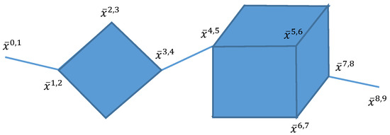
where $E\left(g\left({\overline{r}}_1\right)\right)$, $E\left(g\left({\overline{r}}_4\right)\right)$ and $E\left(g\left({\overline{r}}_8\right)\right)$ are one-dimensional polytopes, $E\left(g\left({\overline{r}}_2\right)\right)$ is a two-dimensional polytope, and $E\left(g\left({\overline{r}}_5\right)\right)$ is a three-dimensional polytope. Moreover, we get $E\left(g\left({\overline{r}}_1\right)\right)\bigcap E\left(g\left({\overline{r}}_2\right)\right)=\left\{{\overline{x}}^{1,2}\right\}$, $E\left(g\left({\overline{r}}_2\right)\right)\bigcap E\left(g\left({\overline{r}}_4\right)\right)=\left\{{\overline{x}}^{3,4}\right\}$, $E\left(g\left({\overline{r}}_4\right)\right)\bigcap E\left(g\left({\overline{r}}_5\right)\right)=\left\{{\overline{x}}^{4,5}\right\}$ and $E\left(g\left({\overline{r}}_5\right)\right)\bigcap E\left(g\left({\overline{r}}_8\right)\right)=\left\{{\overline{x}}^{7,8}\right\}$, where ${\overline{x}}^{k-1,k}$ is defined by (3) and (4) for all $1\le k\le 9$ when $(r,q)=(\overline{r},\overline{q})$. See Figure 2:

Figure 2. The schematic diagram of $S(\overline{r},\overline{q})$ in Example 1 when ${\overline{r}}_1<{\overline{r}}_2={\overline{r}}_3<{\overline{r}}_4<{\overline{r}}_5={\overline{r}}_6={\overline{r}}_7<{\overline{r}}_8<{\overline{r}}_9$.

The remaining part of this section is to seek $S^w(r,q)$ for the bi-criteria piecewise linear convex program (2). Note that $S(r,q)\subset S^w(r,q)$ always hold. Moreover, since (2) is convex, it follows from (ref. [22], Propositions 3.9 and 3.10) that

$$S^w(r,q)=S(r,q)\bigcup \mathbf{S}\bigcup E\left(0\right),$$

where the set $\mathbf{S}$ consists of all the optimal solutions to the problem

$$\begin{array}{ccc}\hfill \mathrm{minimize}& & \omega \left(x\right)\hfill \\ \hfill \mathrm{subject} \mathrm{to}& & {\displaystyle \sum _{j=1}^n}{x}_j=1,\hfill \\ & & x_j\ge 0,j=1,2,\cdots ,n,\hfill \end{array}$$

(22)

and the set $E\left(0\right)$ consists of all the optimal solutions to the problem

$$\begin{array}{ccc}\hfill \mathrm{minimize}& & -\pi \left(x\right)\hfill \\ \hfill \mathrm{subject} \mathrm{to}& & {\displaystyle \sum _{j=1}^n}{x}_j=1,\hfill \\ & & x_j\ge 0,j=1,2,\cdots ,n.\hfill \end{array}$$

(23)

Remark 4.

The optimal solution set to the problem (23) is $E\left(0\right)=\left\{x\right|x_j=0,if{r}_j<r_{max};$$x_j\ge 0,if{r}_j=r_{max};e^{T}x=1\}$. It is clear that $E\left(0\right)$ is a polytope. Moreover, x is a vertex of $E\left(0\right)$ if and only if there exists some $k\in I_{max}^0\left(r\right)$ such that $x=e_k$, so the number of vertices of $E\left(0\right)$ is $|I_{max}^0\left(r\right)|$. The dimension of $E\left(0\right)$ is $|I_{max}^0\left(r\right)| -1$ and

$$E\left(0\right)\bigcap S(r,q)=\left\{\overline{x}\right\},$$

where ${\overline{x}}_j=0$ if $r_j<r_{max}$ and ${\overline{x}}_j={\displaystyle \frac{1}{q_j}}/{\sum }_{i\in I_{max}^0\left(r\right)}{\displaystyle \frac{1}{q_i}}$ if $r_j=r_{max}$.

Next, we’ll go to seek the analytic derivations of $\mathbf{S}$ in the following propositions.

Proposition 1.

The problem (22) has a unique optimal solution, i.e., $\mathbf{S}$ is singleton, and simultaneously, $\mathbf{S}=\left\{{\left({\displaystyle \frac{1}{q_1}},{\displaystyle \frac{1}{q_2}},\cdots ,{\displaystyle \frac{1}{q_n}}\right)}^T/h\left(r_{min}\right)\right\}$.

Proof. 

According to the optimality condition for convex optimization (ref. [14], Theorem 8.15), x is an optimal solution to (22) if and only if there exists some $\tau \in \mathbb{R}$ such that

$${\displaystyle \sum _{j=1}^n}{x}_j=1,$$

(24)

$$x_j\ge 0,j=1,2,\cdots ,n,$$

and

$$-\tau e\in \partial \omega \left(x\right).$$

We have $x\ne 0$, for otherwise (24) cannot be fulfilled. Since $-\tau e={(-\tau ,-\tau ,\cdots ,-\tau )}^T\in \partial \omega \left(x\right)$, it follows from Lemma 2 that $-\tau >0$, ${\sum }_{j=1}^n{\displaystyle \frac{-\tau }{q_j}}=1$ and $x_j={\displaystyle \frac{\omega \left(x\right)}{q_j}}$ for all $j\in I$. Together with (24), we have $\omega \left(x\right)={\displaystyle \frac{1}{{\sum }_{j=1}^n\frac{1}{q_j}}}={\displaystyle \frac{1}{h\left(r_{min}\right)}}$, which implies $x_j={\displaystyle \frac{1}{q_j}}/h\left(r_{min}\right)$ for all $j\in I$. Thus, $\mathbf{S}=\left\{{\left({\displaystyle \frac{1}{q_1}},{\displaystyle \frac{1}{q_2}},\cdots ,{\displaystyle \frac{1}{q_n}}\right)}^T/h\left(r_{min}\right)\right\}$ is singleton. This completes the proof. □

It follows from Proposition 1 and Corollary 1 that the unique solution to the problem (22) is also a solution to the problem (5), that is, $\mathbf{S}\subset S(r,q)$. Thus,

$$S^w(r,q)=S(r,q)\bigcup E\left(0\right).$$

(25)

This shows that we can also convert the bi-criteria piecewise linear convex program (2) into the following parametric optimization problem to seek $S^w(r,q)$:

$$\mathrm{minimize}\lambda \omega \left(x\right)-\pi \left(x\right)$$

$$\mathrm{subject} \mathrm{to}{\displaystyle \sum _{j=1}^n}{x}_j=1,$$

(26)

$$x_j\ge 0,j=1,2,\cdots ,n,$$

where $\lambda \ge 0$. Note that the function $\lambda \omega \left(x\right)-\pi \left(x\right)$ is a continuous function and the feasible region is a compact set. Thus, the parametric optimization problem (26) has a nonempty optimal solution set $E\left(\lambda \right)$ for all $\lambda \ge 0$.

In view of (25), (26) and Theorems 3, we can immediately summarize the analytic forms of $S^w(r,q)$ in the following theorem whose proof are rather straightforward and thus omitted.

Theorem 4.

Let m be the number of distinct $r_j$’s. Then $S^w(r,q)$ consists of m connected polytopes. Explicitly, we have

$$S^w(r,q)=S(r,q)\bigcup E\left(0\right)=\bigcup _{\lambda \ge 0}E\left(\lambda \right)=\bigcup _{r_k\le r_{max}}E\left(g\left(r_k\right)\right),$$

where the detailed descriptions of $S(r,q)$ and $E\left(0\right)$ can be found in Theorem 3 and Remark 4, respectively. In particular, if $|I_{max}^0\left(r\right)| =1$, we get $S^w(r,q)=S(r,q)$.

To end this section, we give the following example to show that a weakly efficient solution may not necessarily be an efficient solution.

Example 2.

Consider the bi-criteria linear program (2) with $(\overline{r},\overline{q})\in {\mathbb{R}}^n\times {\mathbb{R}}_{++}^n$ satisfying ${\overline{r}}_1<{\overline{r}}_2<{\overline{r}}_3<{\overline{r}}_4={\overline{r}}_5={\overline{r}}_6$. Then we have $S(r,q)=\left[{\overline{x}}^{0,1},{\overline{x}}^{1,2}\right]\cup \left[{\overline{x}}^{1,2},{\overline{x}}^{2,3}\right]\cup \left[{\overline{x}}^{2,3},{\overline{x}}^{3,4}\right]$, where ${\overline{x}}^{k-1,k}$ is defined by (3) and (4) for all $1\le k\le 4$ when $(r,q)=(\overline{r},\overline{q})$. Simultaneously, we get $S^w(r,q)=S(r,q)\bigcup \mathrm{conv}\{e_4,e_5,e_6\}$. Thus, $S(r,q)$ is a proper subset of $S^w(r,q)$.

4. Stabilities of Efficient and Weakly Efficient Solution Set Mappings

The analytic forms and properties of the efficient solution set established in Section 3 lead to the following key conclusions for our stability analysis:

Lemma 3.

Let $(r,q)\in {\mathbb{R}}^n\times {\mathbb{R}}_{++}^n$.

(a) 

Then $S(r,q)$ is the union of a finite number of polytopes, which implies that $S(r,q)$ is a compact set. Thus, S is nonempty-compact-valued on ${\mathbb{R}}^n\times {\mathbb{R}}_{++}^n$.

(b) 

The efficient solution set $S(r,q)$ is determined by the order of the components of r and the value of q. In particular, if $O\left(r\right)=O\left(\overline{r}\right)$, that is, the components of r and $\overline{r}$ have the same order, we get $S(r,q)=S(\overline{r},q)$ for all $q\in {\mathbb{R}}_{++}^n$.

(c) 

Let $\overline{r}\in {\mathbb{R}}^n$ with $|I_{max}^0\left(\overline{r}\right)| =1$. Then there exists a small enough neighborhood V of $\overline{r}$ such that $S(r,q)\subset S(\overline{r},q),\forall r\in V,\forall q\in {\mathbb{R}}_{++}^n$.

In the sequel, let $S:{\mathbb{R}}^n\times {\mathbb{R}}_{++}^n\rightrightarrows {\mathbb{R}}^n$ be the efficient solution set mapping of the bi-criteria linear program (2), which is

$$S(r,q):=\bigcup _{r_k<r_{max}}E\left(g\left(r_k\right)\right),\forall (r,q)\in {\mathbb{R}}^n\times {\mathbb{R}}_{++}^n,$$

where $E\left(g\left(r_k\right)\right)$ is the nonempty optimal solution set of the parametric optimization problem (5) when $\lambda =g\left(r_k\right)$ with $r_k<r_{max}$. Simultaneously, let $S^w:{\mathbb{R}}^n\times {\mathbb{R}}_{++}^n\rightrightarrows {\mathbb{R}}^n$ be the weakly efficient solution set mapping of (2), which is defined by

$$S^w(r,q)=\bigcup _{r_k\le r_{max}}E\left(g\left(r_k\right)\right),$$

where $E\left(g\left(r_k\right)\right)$ is the nonempty optimal solution set of the parametric optimization problem (26) when $\lambda =g\left(r_k\right)$ with $r_k\le r_{max}$.

For the sake of simplicity, we define $F:{\mathbb{R}}^n\times {\mathbb{R}}_{++}^n\to {\mathbb{R}}^n$ by

$$F(\theta ,y)={\displaystyle \sum _{j=1}^n}\left({\displaystyle \frac{{\theta }_j/y_j}{{\sum }_{i=1}^n\frac{{\theta }_i}{y_i}}}\right)e_j,$$

where the domain of F is $\mathrm{dom}F=\left\{(\theta ,y)\in {\mathbb{R}}^n\times {\mathbb{R}}_{++}^n|{\sum }_{i=1}^n{\displaystyle \frac{{\theta }_i}{y_i}}\ne 0\right\}$. Given $(r,q)\in {\mathbb{R}}^n\times {\mathbb{R}}_{++}^n$, let $x\in S(r,q)$. Then it follows from Corollary 1 and Theorem 3 that there exists some $\theta \in {[0,1]}^n$ and $\theta \ne 0$ such that $x=F(\theta ,q)$. We observe that the Jacobian of F with respect to y always exists for all $y\in {\mathbb{R}}_{++}^n$, and simultaneously,

$$\begin{array}{c}\hfill \parallel {\nabla }_y{F(\theta ,y)\parallel }_2\le \sqrt{n}\left({\displaystyle \sum _{j=1}^n}{\displaystyle \frac{1}{y_j}}\right),\end{array}$$

where $\parallel {\nabla }_y{F(\theta ,y)\parallel }_2$ denotes the 2-norm of the Jacobian matrix ${\nabla }_{y}F(\theta ,y)$.

Theorem 5.

Let $(\overline{r},\overline{q})\in {\mathbb{R}}^n\times {\mathbb{R}}_{++}^n$. Then the efficient solution set mapping S is outer semicontinuous at $(\overline{r},\overline{q})$ if and only if $|I_{max}^0\left(\overline{r}\right)| =1$.

Proof. 

Let $|I_{max}^0\left(\overline{r}\right)| =1$. Suppose that $(r^v,q^v)\in {\mathbb{R}}^n\times {\mathbb{R}}_{++}^n$, $(r^v,q^v)\to (\overline{r},\overline{q})$ and $S(r^v,q^v)\to D$. Take an arbitrary $x\in D$. Then there exists $x^v\in S(r^v,q^v)$ such that $x^v\to x$. Since $r^v\to \overline{r}$ and $|I_{max}^0\left(\overline{r}\right)| =1$, it follows from Lemma 3(c) that

$$S(r^v,q^v)\subset S(\overline{r},q^v)$$

(27)

holds for sufficiently large $v\in \mathbb{N}$. Note that $q^v\to \overline{q}$. Then we have $S(\overline{r},q^v)\to S(\overline{r},\overline{q})$. Together with $x^v\in S(r^v,q^v)$ and (27), we get $x\in S(\overline{r},\overline{q})$, which implies $D\subset S(\overline{r},\overline{q})$. Thus, S is outer semicontinuous at $(\overline{r},\overline{q})$.

Conversely, let S be outer semicontinuous at $(\overline{r},\overline{q})$. Suppose by contradiction that $|I_{max}^0\left(\overline{r}\right)| \ge 2$. Without loss of generality, assume that $(\overline{r},\overline{q})\in {\mathbb{R}}^n\times {\mathbb{R}}_{++}^n$ with ${\overline{r}}_1\le {\overline{r}}_2\le \cdots \le {\overline{r}}_n$. Then we have $I_{max}^0\left(\overline{r}\right)=\{j\in I|{\overline{r}}_j={\overline{r}}_n\}$. Let $|I_{max}^0\left(\overline{r}\right)| =m$. It follows that $m\ge 2$ and $I_{max}^0\left(\overline{r}\right)=\{n-m+1,n-m+2,\cdots ,n\}$. Together with Theorem 3, we get

$$S(\overline{r},\overline{q})={\displaystyle \bigcup _{k=1}^{n-m}}E\left(g\left({\overline{r}}_k\right)\right).$$

(28)

Let $(r^v,q^v)\to (\overline{r},\overline{q})$ with $r_1^v<r_2^v<\cdots <r_{n-1}^v<r_n^v$. Then it follows from Theorems 1–3 that $S(r^v,q^v)={\bigcup }_{k=1}^{n-1}\left[{\left(x^v\right)}^{k-1,k},{\left(x^v\right)}^{k,k+1}\right]$, where ${\left(x^v\right)}^{k-1,k}$ is defined by (3) and (4) for all $1\le k\le n$ when $(r,q)=(r^v,q^v)$. Let $D={\bigcup }_{k=1}^{n-1}\left[{\overline{x}}^{k-1,k},{\overline{x}}^{k,k+1}\right]$, where ${\overline{x}}^{k-1,k}$ is defined by (3) and (4) for all $1\le k\le n$ when $(r,q)=(\overline{r},\overline{q})$. Then, it is clear that $S(r^v,q^v)\to D$ since $q^v\to \overline{q}$. Note that ${\overline{x}}^{n-1,n}\in D$. Simultaneously, it follows from $m\ge 2$ and (28) that ${\overline{x}}^{n-1,n}\notin S(\overline{r},\overline{q})$. Thus, we have $D\neg \subset S(\overline{r},\overline{q})$. This shows that S is not outer semicontinuous at $(\overline{r},\overline{q})$. This completes the proof. □

Theorem 6.

Let $(\overline{r},\overline{q})\in {\mathbb{R}}^n\times {\mathbb{R}}_{++}^n$. Then the efficient solution set mapping S is inner semicontinuous at $(\overline{r},\overline{q})$ if and only if $|I^0(\overline{r},k)| =1$ for all ${\overline{r}}_k<{\overline{r}}_{max}$.

Proof. 

Let $|I^0(\overline{r},k)| =1$ for all ${\overline{r}}_k<{\overline{r}}_{max}$. Without loss of generality, suppose that ${\overline{r}}_1<{\overline{r}}_2<\cdots <{\overline{r}}_{m-1}<{\overline{r}}_m={\overline{r}}_{m+1}=\cdots ={\overline{r}}_n$ and $m\le n$. Let $(r^v,q^v)\to (\overline{r},\overline{q})$ and $S(r^v,q^v)\to D$. Next, we consider the following two possible cases:

In the case $m=n$, we have ${\overline{r}}_1<{\overline{r}}_2<\cdots <{\overline{r}}_{n-1}<{\overline{r}}_n$. Since $r^v\to \overline{r}$, we get $r_1^v<r_2^v<\cdots <r_{n-1}^v<r_n^v$ for sufficiently large $v\in \mathbb{N}$. It follows from Theorems 1 and 3 that $D=S(\overline{r},\overline{q})$. Thus, S is inner semicontinuous at $(\overline{r},\overline{q})$.

In the case $m<n$, we have ${\overline{r}}_1<{\overline{r}}_2<\cdots <{\overline{r}}_m={\overline{r}}_{m+1}=\cdots ={\overline{r}}_n$, which implies $r_1^v<r_2^v<\cdots <r_m^v$ for sufficiently large $v\in \mathbb{N}$. It follows from Corollary 1 and Theorem 3 that $S(\overline{r},\overline{q})\subset D$. Thus, S is inner semicontinuous at $(\overline{r},\overline{q})$.

Conversely, suppose by contradiction that there exists $k\in I$ with ${\overline{r}}_k<{\overline{r}}_{max}$ such that $|I^0(\overline{r},k)| \ge 2$. Without loss of generality, assume that ${\overline{r}}_1\le {\overline{r}}_2\le \cdots \le {\overline{r}}_n$. For simplicity, we denote by $\xi \left(k\right)=min{I}^0(\overline{r},k)$ and $\eta \left(k\right)=max{I}^0(\overline{r},k)$. Let $\overline{x}=F(\overline{\theta },\overline{q})$ with ${\overline{\theta }}_j=1$ for $j\in \left\{\xi \right(k),\eta (k)+1,\cdots ,n\}$ and ${\overline{\theta }}_j=0$ for $j\in I\setminus \left\{\xi \right(k),\eta (k)+1,\cdots ,n\}$. It follows from Theorems 1 and 3 that $\overline{x}\in S(\overline{r},\overline{q})$. Take arbitrarily $(r^v,q^v)\to (\overline{r},\overline{q})$ with $r_1^v<r_2^v<\cdots <r_n^v$. Then we have $S(r^v,q^v)\to D$, where $D={\bigcup }_{k=1}^{n-1}\left[{\overline{x}}^{k-1,k},{\overline{x}}^{k,k+1}\right]$, where ${\overline{x}}^{k-1,k}$ is defined by (3) and (4) for all $1\le k\le n$ when $(r,q)=(\overline{r},\overline{q})$. Obviously, we have $\overline{x}\notin D$ since $|I^0(\overline{r},k)| \ge 2$. Thus, S is not inner semicontinuous at $(\overline{r},\overline{q})$. This completes the proof. □

Combining Theorems 5 and 6, we can get the following result.

Theorem 7.

Let $(\overline{r},\overline{q})\in {\mathbb{R}}^n\times {\mathbb{R}}_{++}^n$. Then the efficient solution set mapping S is continuous at $(\overline{r},\overline{q})$ if and only if ${\overline{r}}_i\ne {\overline{r}}_j$ for all $i\ne j$.

Next, we provide the following result to show the Lipschitz continuity of the efficient solution set mapping S.

Theorem 8.

Let $(\overline{r},\overline{q})\in {\mathbb{R}}^n\times {\mathbb{R}}_{++}^n$ and $\Omega =\{r\in {\mathbb{R}}^n|O\left(r\right)=O\left(\overline{r}\right)\}$. Then there are a neighborhood V of $\overline{q}$ and a real number $L>0$ such that

$$d_{\infty }\left(S(r,q),S(\tilde{r},\tilde{q})\right)\le L\parallel q-\tilde{q}\parallel ,\forall (r,q),(\tilde{r},\tilde{q})\in \Omega \times V,$$

that is, the efficient solution set mapping S is Lipschitz continuous on $\Omega \times V$.

Proof. 

We observe from Lemma 3(a) that S is nonempty-compact-valued on ${\mathbb{R}}^n\times {\mathbb{R}}_{++}^n$. Let $r,\tilde{r}\in \Omega$ and $q,\tilde{q}\in {\mathbb{R}}_{++}^n$. Note that for every $\tilde{x}\in S(\tilde{r},\tilde{q})$, there exists $\tilde{\theta }\in {[0,1]}^n$ and $\tilde{\theta }\ne 0$ such that $\tilde{x}=F(\tilde{\theta },\tilde{q}).$ Take $x=F(\tilde{\theta },q)$. Since $O\left(r\right)=O\left(\tilde{r}\right)$, it follows from Corollary 1, Theorem 3 and Lemma 3(b) that $x\in S(r,q)$, and then $d\left(\tilde{x};S(r,q)\right)\le \parallel \tilde{x}-x\parallel =\parallel F(\tilde{\theta },\tilde{q})-F(\tilde{\theta },q)\parallel .$ Note that F is continuously differentiable at $\overline{q}\in {\mathbb{R}}_{++}^n$ with respect to q for all $\theta \in {[0,1]}^n$ and $\theta \ne 0$. Then it follows from (ref. [14], Theorem 9.7) that there exists a neighborhood V of $\overline{q}$ such that

$$\parallel F(\tilde{\theta },\tilde{q})-F(\tilde{\theta },q)\parallel \le \Vert {\nabla }_{q}F(\tilde{\theta },\overline{q})\Vert \parallel \tilde{q}-q\parallel \le \sqrt{n}\left({\displaystyle \sum _{j=1}^n}{\displaystyle \frac{1}{{\overline{q}}_j}}\right)\parallel \tilde{q}-q\parallel ,\forall q,\tilde{q}\in V.$$

Thus, we have $d(\tilde{x};S(r,q))\le \sqrt{n}\left({\sum }_{j=1}^n{\displaystyle \frac{1}{{\overline{q}}_j}}\right)\parallel \tilde{q}-q\parallel$ for $\tilde{x}\in S(\tilde{r},\tilde{q})$, which implies

$$\underset{z\in S(\tilde{r},\tilde{q})}{sup}d\left(z;S(r,q)\right)\le \sqrt{n}\left({\displaystyle \sum _{j=1}^n}{\displaystyle \frac{1}{{\overline{q}}_j}}\right)\parallel \tilde{q}-q\parallel ,\forall q,\tilde{q}\in V.$$

Similarly, it can be concluded that

$$\underset{y\in S(r,q)}{sup}d\left(y;S(\tilde{r},\tilde{q})\right)\le \sqrt{n}\left({\displaystyle \sum _{j=1}^n}{\displaystyle \frac{1}{{\overline{q}}_j}}\right)\parallel q-\tilde{q}\parallel ,\forall q,\tilde{q}\in V.$$

Let $L:=\sqrt{n}\left({\sum }_{j=1}^n{\displaystyle \frac{1}{{\overline{q}}_j}}\right)$. Then we get

$$\begin{array}{ccc}\hfill d_{\infty }\left(S(r,q),S(\tilde{r},\tilde{q})\right)& =& max\left\{\underset{z\in S(\tilde{r},\tilde{q})}{sup}d\left(z;S(r,q)\right),\underset{y\in S(r,q)}{sup}d\left(y;S(\tilde{r},\tilde{q})\right)\right\}\hfill \\ & \le & \sqrt{n}\left({\displaystyle \sum _{j=1}^n}{\displaystyle \frac{1}{{\overline{q}}_j}}\right)\parallel q-\tilde{q}\parallel \hfill \\ & =& L\parallel q-\tilde{q}\parallel ,\forall (r,q),(\tilde{r},\tilde{q})\in \Omega \times V.\hfill \end{array}$$

This completes the proof. □

Remark 5.

Theorem 7 shows that even if there are errors in the estimated parameters, as long as the components of r are different from each other and the estimated parameter $(r,q)$ is close enough to $(\overline{r},\overline{q})$, the solution set obtained from the model is close to the exact solution set, that is, the model has stability. Theorem 8 shows that even if the estimated parameters $(r,q)$ and $(\tilde{r},\tilde{q})$ of $(\overline{r},\overline{q})$ have errors, as long as the structures of the components of the two estimated parameters r and $\tilde{r}$ remain consistent with $\overline{r}$, and the estimated parameters q and $\tilde{q}$ are close enough to $\overline{q}$, the change in the distance between the two solution sets obtained from this model can be controlled by $L\parallel q-\tilde{q}\parallel$. This implies that the stability of the model depends on global change in r and local change in q.

In view of Theorems 1–8, we can immediately obtain the stability results of the weakly efficient solution set mapping $S^w$ in the following theorem whose proof is rather similar and thus omitted.

Theorem 9.

Let $(\overline{r},\overline{q})\in {\mathbb{R}}^n\times {\mathbb{R}}_{++}^n$. Then the following statements hold:

(a) 

$S^w$ is outer semicontinuous at $(\overline{r},\overline{q})$.

(b) 

$S^w$ is inner semicontinuous at $(\overline{r},\overline{q})$ if and only if ${\overline{r}}_i\ne {\overline{r}}_j$ for all $i\ne j$.

(c) 

$S^w$ is continuous at $(\overline{r},\overline{q})$ if and only if ${\overline{r}}_i\ne {\overline{r}}_j$ for all $i\ne j$.

(d) 

$S^w$ is Lipschitz continuous on $\Omega \times V$, where $\Omega =\{r\in {\mathbb{R}}^n|O\left(r\right)=O\left(\overline{r}\right)\}$ and V is a neighborhood of $\overline{q}$.

5. Numerical Simulations

To verify the preceding theory, this section conducts numerical simulations to visually demonstrate the structure and stability of the model’s efficient portfolios.

Example 3.

In this experiment, assume investing in only seven risky assets. Given the values of $\overline{r}$ and $\overline{q}$, calculate the corresponding ${\overline{x}}^{k-1,k},j=1,2,3,4,5,6,7$, where ${\overline{x}}^{k-1,k}$ is defined by Equations (3) and (4). These values are presented in the table below. Consider seven risky assets with expected returns and absolute deviations as shown in Table 1.

Table 1. Asset Information.

Asset j	1	2	3	4	5	6	7
Expected Return ${\overline{r}}_j$	0.05	0.10	0.15	0.15	0.20	0.25	0.30
Absolute Deviation ${\overline{q}}_j$	0.01	0.012	0.018	0.019	0.023	0.029	0.033

According to theoretical formulas, the ${\overline{x}}_j^{k-1,k},j=1,2,3,4,5,6,7$ are computed as shown in Table 2, where $x_1,x_2,x_3,x_4,x_5,x_6,x_7$, represent the seven components of ${\overline{x}}^{k-1,k}$, respectively. The computed risk–return for each portfolio and weights are shown in Table 2.

Table 2. Portfolio risk, return and weights.

Portfolio	$\mathit{\lambda }$	${\overline{\mathit{x}}}_1^{\mathit{k}-1,\mathit{k}}$	${\overline{\mathit{x}}}_2^{\mathit{k}-1,\mathit{k}}$	${\overline{\mathit{x}}}_3^{\mathit{k}-1,\mathit{k}}$	${\overline{\mathit{x}}}_4^{\mathit{k}-1,\mathit{k}}$	${\overline{\mathit{x}}}_5^{\mathit{k}-1,\mathit{k}}$	${\overline{\mathit{x}}}_6^{\mathit{k}-1,\mathit{k}}$	${\overline{\mathit{x}}}_7^{\mathit{k}-1,\mathit{k}}$	$\mathit{\omega }\left(\mathit{x}\right)$	$\mathit{\pi }\left(\mathit{x}\right)$
${\overline{x}}^{0,1}$	18.0000	0.250	0.208	0.139	0.132	0.109	0.086	0.076	0.0025	0.0500
${\overline{x}}^{1,2}$	13.3333	0.000	0.278	0.185	0.176	0.145	0.115	0.101	0.0033	0.1000
${\overline{x}}^{2,3}$	8.8889	0.000	0.000	0.257	0.243	0.201	0.159	0.140	0.0046	0.1500
${\overline{x}}^{3,4}$	6.6667	0.000	0.000	0.000	0.327	0.270	0.215	0.188	0.0062	0.1500
${\overline{x}}^{4,5}$	5.0000	0.000	0.000	0.000	0.000	0.402	0.318	0.280	0.0092	0.2000
${\overline{x}}^{5,6}$	3.3333	0.000	0.000	0.000	0.000	0.000	0.532	0.468	0.0154	0.2500
${\overline{x}}^{6,7}$	2.0000	0.000	0.000	0.000	0.000	0.000	0.000	1.000	0.0330	0.3000

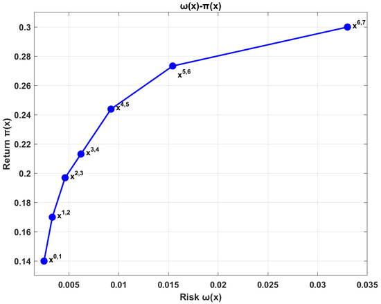
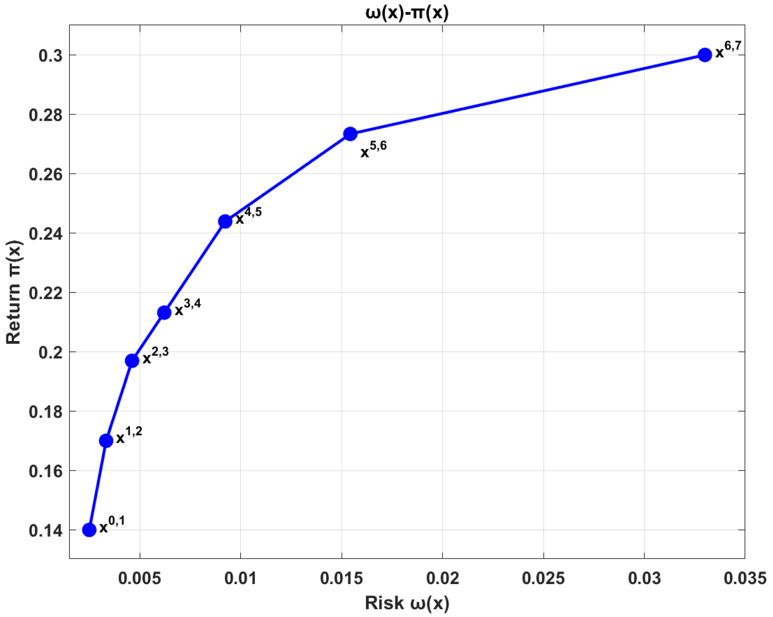
Figure 3 illustrates the efficient frontier computed based on the bi-criteria portfolio optimization model. This figure depicts the distribution of different portfolios in the risk–return plane.

Figure 3. Relationship between risk $\omega \left(x\right)$ and return $\pi \left(x\right)$.

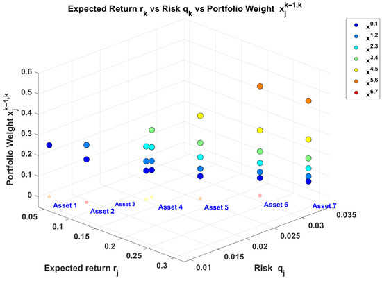
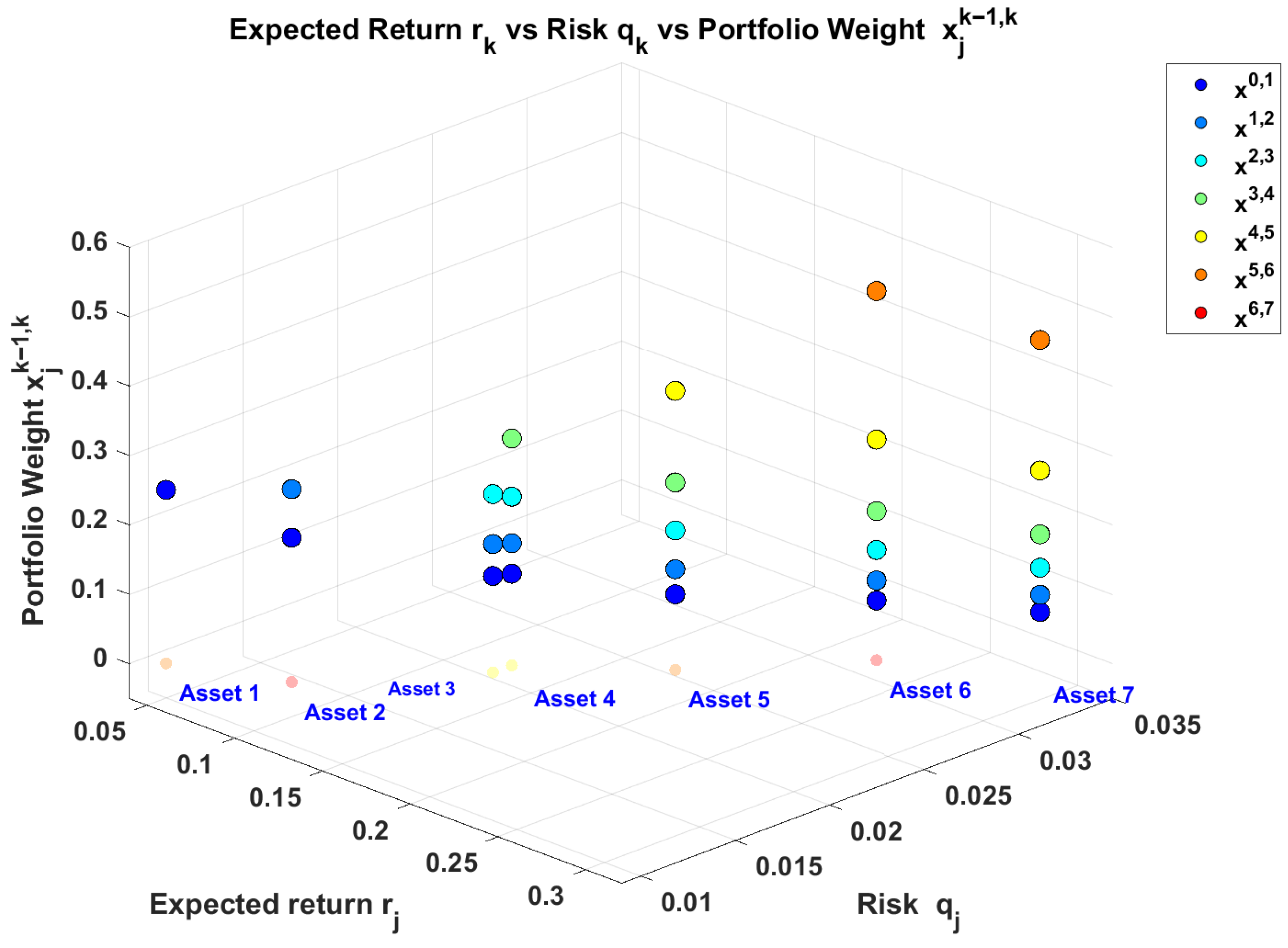
Figure 4 demonstrates the relationship between three key dimensions of assets in the portfolio. Each portfolio is identified by a different color. From left to right, we can observe the transition from conservative to aggressive portfolios. The $x^{0,1}$ contains all assets, while $x^{6,7}$ contains only asset seven.

Figure 4. Relationship between expected return, risk and weight.

Example 4.

Suppose only seven risky assets are considered for investment, and given the two sets of values of $(\overline{r},\overline{q})$, as shown in the following Table 3 and Table 4.

Table 3. Case1: Parameter Settings.

Asset j	1	2	3	4	5	6	7
${\overline{r}}_j$	0.05	0.10	0.15	0.18	0.20	0.25	0.30
${\overline{q}}_j$	0.01	0.012	0.018	0.019	0.023	0.029	0.033

Table 4. Case2: Parameter Settings.

Asset j	1	2	3	4	5	6	7
${\overline{r}}_j$	0.05	0.10	0.15	0.18	0.20	0.25	0.25
${\overline{q}}_j$	0.01	0.012	0.018	0.019	0.023	0.029	0.033

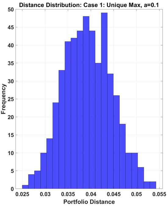
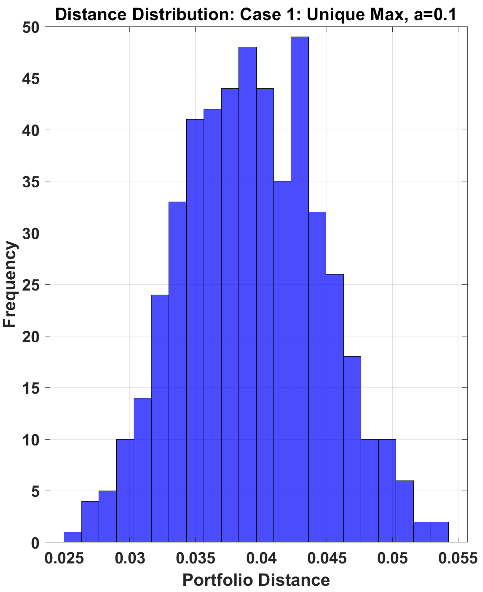
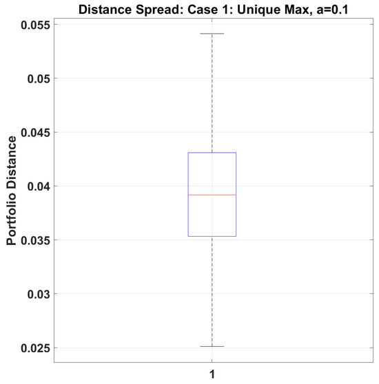
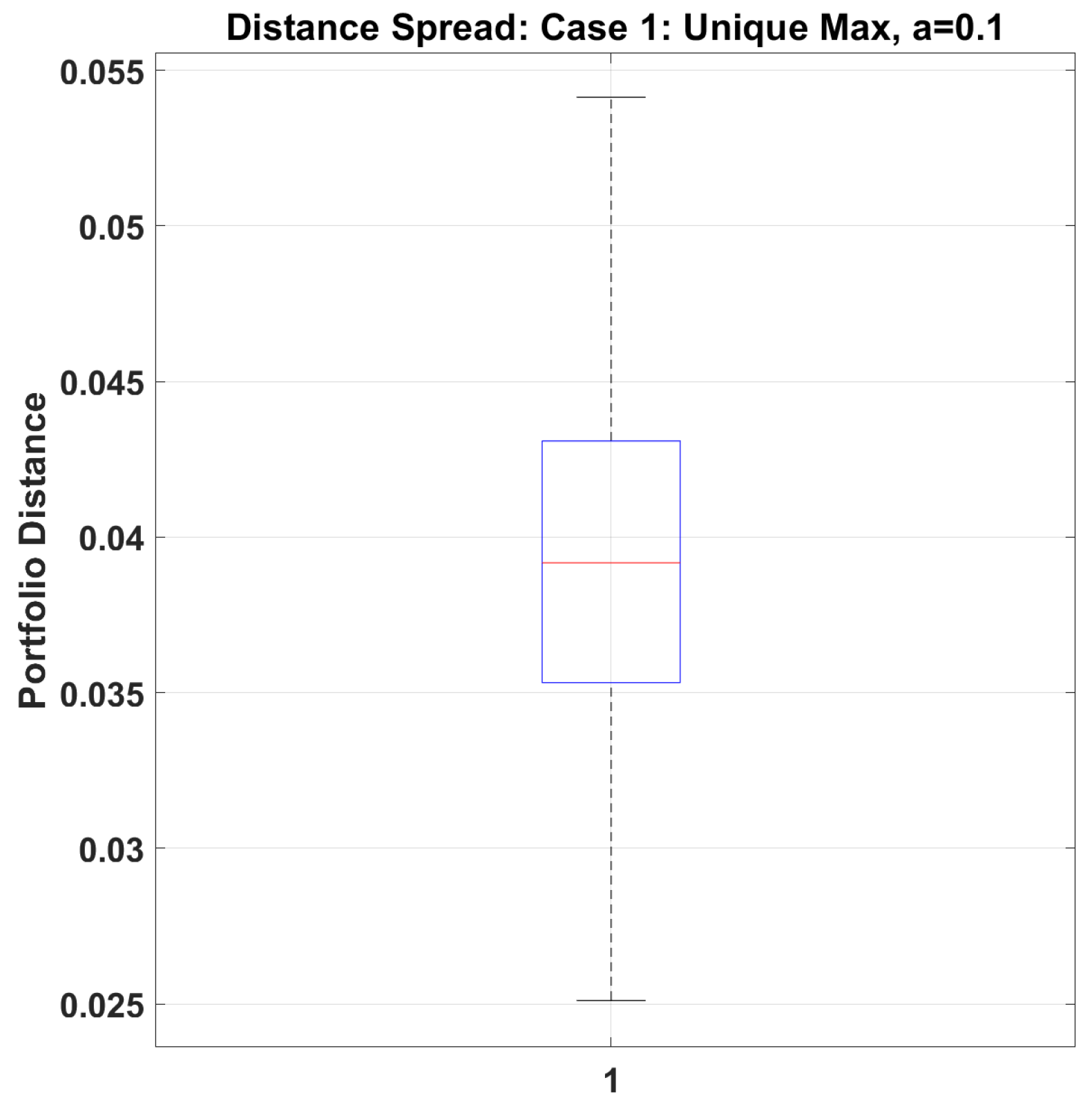
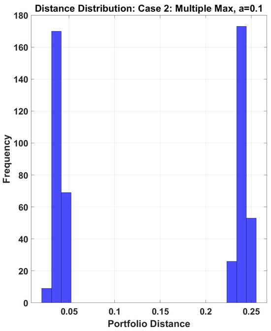
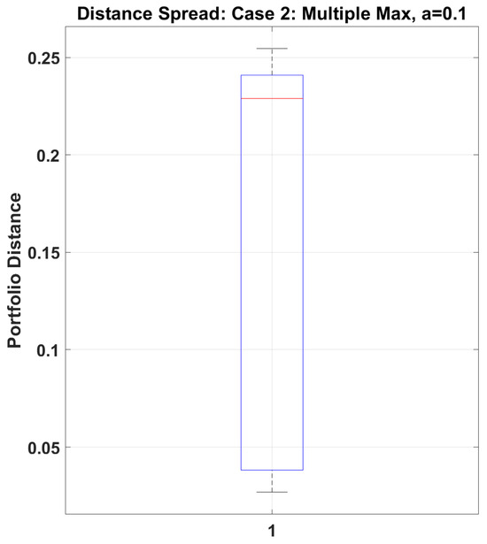
Adopting the Monte Carlo simulation method. Generate perturbed parameters $(r,q)$ within intervals: $r_j\in [{\overline{r}}_j-0.1a,{\overline{r}}_j+0.1a]$, $q_j\in [{\overline{q}}_j-a{\overline{q}}_j,{\overline{q}}_j+a{\overline{q}}_j$, where a is a positive integer. A total of 1500 values were selected. Let $u:=({\overline{x}}^{0,1},{\overline{x}}^{1,2},{\overline{x}}^{2,3},{\overline{x}}^{3,4},{\overline{x}}^{4,5},{\overline{x}}^{5,6},{\overline{x}}^{6,7}).$ Based on each simulation experiment, we can obtain the vector v representing the composition of the new investment portfolio, which takes the specific form: $v:=(x\left({\theta }_1\right),x\left({\theta }_2\right),x\left({\theta }_3\right),x\left({\theta }_4\right),x\left({\theta }_5\right),x\left({\theta }_6\right),x\left({\theta }_7\right))$, where all components in ${\theta }_1$ are 1; for ${\theta }_2$, the components corresponding to the six risk assets with higher investment returns are 1, and the rest are 0; for ${\theta }_3$, the components corresponding to the five risk assets with higher investment returns are 1, and the rest are 0; for ${\theta }_4$, ${\theta }_5$, ${\theta }_6$, ${\theta }_7$, the above rules are still followed for assignment. For $j\in \{1,2,3,4,5,6,7\}$, we employ $d(u,v)={\sum }_{j=1}^7\sqrt{{\sum }_{i=1}^7{(u_i^j-v_i^j)}^2}$ calculate the distance between u and v. Take $a=0.1$ and $a=0.9$, respectively, we can get the following table (Table 5).

Table 5. Monte Carlo Simulation Results Statistics.

Test Case	Perturbation a	Max Distance	Mean Distance	Std Dev
Case 1 (Unique Max)	0.1	0.045	0.018	0.008
Case 1 (Unique Max)	0.9	0.152	0.067	0.032
Case 2 (Multiple Max)	0.1	0.238	0.089	0.045
Case 2 (Multiple Max)	0.9	0.563	0.234	0.121

From the experimental results, we observe the following: for the Case 1, when $a=0.1$, portfolio distances concentrate in a small range, when $a=0.9$, distance distribution remains relatively concentrated with small standard deviation; for Case 2, even with small perturbations ($a=0.1$), large distances occur (maximum 0.238) and Distance distribution is dispersed with large standard deviation. Indicates the solution set mapping in Case 1 is insensitive to external perturbations, but the solution set mapping in Case 2 is sensitive to perturbations. This implies that when there exists a unique maximum return asset, small parameter perturbations only cause small changes in the solution set; when multiple assets share the maximum return, even small parameter perturbations may lead to significant changes in the solution set (see Figure 5, Figure 6, Figure 7 and Figure 8).

Figure 5. Case 1, a = 0.1.

Figure 6. Case 1, a = 0.1.

Figure 7. Case 2, a = 0.1.

Figure 8. Case 2, a = 0.1.

6. Conclusions

In this paper, we present an in-depth qualitative analysis of this model in terms of the continuity of set-valued maps. Specifically, we first derive explicit analytical expressions for all efficient and weakly efficient portfolios and thoroughly examine their structural properties, such as dimensionality and distribution. Building on this, we systematically establish outer semicontinuity, inner semicontinuity, and Lipschitz continuity for the efficient and weakly efficient solution set mappings. These results characterize the stability of the model’s solutions from different angles. The theoretical achievements enhance our understanding of the impact of parameter perturbations on the model and offer a solid theoretical foundation for investors to select robust investment strategies in uncertain environments.

This approach could be applied to other optimization problems that yield a similarly piecewise linear efficient frontier, such as those with the ${\mathcal{l}}_1$ risk. However, for more complex risk measures, the efficient frontier is typically nonlinear, which makes it exceedingly difficult to obtain complete analytical solutions and thus limits the direct application of our method. This study demonstrates that for an important class of optimization problems with clear geometric structures, stability analysis based on analytical solutions is a viable and informative approach. It provides qualitative guarantees of the model’s behavior under perturbation. These insights can help guide the construction of more stable models in future work. Future work will be dedicated to analyzing the solution set characteristics and stability of mean absolute deviation risk models and models that incorporate general risk measures.

References

- Markowitz, H.M. Portfolio selection. J. Financ. 1952, 7, 77–91. [Google Scholar]
- Campbell, R.; Huisman, R.; Koedijk, K. Optimal portfolio selection in a Value-at-Risk framework. J. Bank. Financ. 2001, 25, 1789–1804. [Google Scholar] [CrossRef] [Scilit]
- Cai, X.Q.; Teo, K.L.; Yang, X.Q.; Zhou, X.Y. Portfolio optimization under a minimax rule. Manag. Sci. 2000, 46, 957–972. [Google Scholar] [CrossRef] [Scilit]
- Konno, H. Piecewise linear risk function and portfolio optimization. J. Oper. Res. Soc. Jpn. 1990, 33, 139–156. [Google Scholar] [CrossRef] [Scilit]
- Meng, K.W.; Yang, H.Y.; Yang, X.Q.; Yu, C.K.W. Portfolio optimization under a minimax rule revisited. Optimization 2022, 71, 877–905. [Google Scholar] [CrossRef] [Scilit]
- Rockafellar, R.T.; Uryasev, S. Optimization of conditional value-at-risk. J. Risk 2000, 2, 21–42. [Google Scholar] [CrossRef] [Scilit]
- Speranza, G.M. Linear programming models for portfolio optimization. Finance 1993, 14, 107–123. [Google Scholar]
- Chopra, V.K.; Hensel, C.R.; Turner, A.L. Massaging mean-variance inputs: Returns from alternative global investment strategies in the 1980s. Manag. Sci. 1993, 39, 845–855. [Google Scholar] [CrossRef] [Scilit]
- Chopra, V.K.; Ziemba, W.T. The effect of errors in means, variances, and covariances on optimal portfolio choice. J. Portf. Manag. 1993, 19, 6–11. [Google Scholar] [CrossRef] [Scilit]
- Kondor, I.; Pafka, S.; Nagy, G. Noise sensitivity of portfolio selection under various risk measures. J. Bank. Financ. 2007, 31, 1545–1573. [Google Scholar] [CrossRef] [Scilit]
- Luc, D.T. Theory of Vector Optimization; Lecture Notes in Economics and Mathematical Systems; Springer: Berlin/Heidelberg, Germany, 1989. [Google Scholar]
- Luc, D.T. Multiobjective Linear Programming: An Introduction; Springer: Berlin/Heidelberg, Germany, 2016. [Google Scholar]
- Mordukhovich, B.S. Variational Analysis and Generalized Differentiation, Volume I: Basic Theory; Springer: Berlin/Heidelberg, Germany, 2006. [Google Scholar]
- Rockafellar, R.T.; Wets, R.J.B. Variational Analysis; Springer: Berlin/Heidelberg, Germany, 1998. [Google Scholar]
- Cheng, Y.H.; Zhu, D.L. Global stability results for the weak vector variational inequality. J. Glob. Optim. 2005, 32, 543–550. [Google Scholar] [CrossRef] [Scilit]
- Han, Y. Lipschitz continuity of approximate solution mappings to parametric generalized vector equilibrium problems. J. Optim. Appl. 2018, 178, 763–793. [Google Scholar] [CrossRef] [Scilit]
- Li, S.J.; Chen, G.Y.; Teo, K.L. On the stability of generalized vector quasivariational inequality problems. J. Optim. Theory Appl. 2002, 113, 283–295. [Google Scholar] [CrossRef] [Scilit]
- Zhao, J.G. The lower semicontinuity of optimal solution sets. J. Math. Anal. Appl. 1997, 207, 240–254. [Google Scholar] [CrossRef] [Scilit]
- Cheng, T.Y.; Chen, K. A general framework for portfolio construction based on generative models of asset returns. J. Financ. Data Sci. 2023, 9, 100–113. [Google Scholar] [CrossRef] [Scilit]
- Li, J.Y.M. Wasserstein-Kelly Portfolios: A robust data-driven solution to optimize portfolio growth. arXiv 2023, arXiv:2302.13979. [Google Scholar] [CrossRef] [Scilit]
- Pan, S.M.; Lu, S.K.; Meng, K.W.; Zhu, S.K. Trade-off ratio functions for linear and piecewise linear multi-objective optimization problems. J. Optim. Theory Appl. 2021, 188, 402–419. [Google Scholar] [CrossRef] [Scilit]
- Ehrgott, M. Multicriteria Optimization; Springer: Berlin/Heidelberg, Germany, 2005. [Google Scholar]
Disclaimer/Publisher’s Note: The statements, opinions and data contained in all publications are solely those of the individual author(s) and contributor(s) and not of MDPI and/or the editor(s). MDPI and/or the editor(s) disclaim responsibility for any injury to people or property resulting from any ideas, methods, instructions or products referred to in the content. |
© 2025 by the authors. Licensee MDPI, Basel, Switzerland. This article is an open access article distributed under the terms and conditions of the Creative Commons Attribution (CC BY) license (https://creativecommons.org/licenses/by/4.0/).