Comparative Study of Estimation Methods for a New Family of Copula-Based Reversible Markov Chains

Abstract

This work explores continuous state–space stationary reversible Markov chains generated by a new family of absolutely continuous symmetric copulas that have piecewise constant densities. We compare three parameter estimation techniques for the Markov chains generated by these copulas. Furthermore, we provide the Central Limit Theorems, ${\chi }^2$-tests and confidence intervals based on these estimators. A simulation study performed using R 4.4.1 is described to support the findings.

1. Introduction

In many areas of research, fitting an appropriate model to capture the dependence in real data is a major issue. A copula helps in capturing the strength of the dependence between random variables, and is a joint cumulative distribution function introduced in Sklar [1]. As defined in Nelsen [2], a bivariate copula is defined as a function $C:{[0,1]}^2\to [0,1]$ for which the following holds:

• For all $u\in [0,1]$, $C(u,0)=C(0,u)=0$ and $C(u,1)=C(1,u)=u.$
• For all $u_1,u_2,v_1,v_2\in [0,1]$, such that $u_1\le u_2$ and $v_1\le v_2$; then,

  $$C(u_2,v_2)-C(u_2,v_1)-C(u_1,v_2)+C(u_1,v_1)\ge 0.$$

Sklar’s Theorem popularized the use of copulas in modeling dependence in various fields of research. It states that, if $H(u,v)$ is the joint distribution of random variables U and V with marginal distributions of $F_U$ and $F_V$, respectively, then there exists a copula $C(·,·)$, such that

$$H(u,v)=C(F_U\left(u\right),F_V\left(v\right)).$$

There are several families of copulas (see Nelsen [2]) that can be used to describe different types of dependencies between random variables. Lower-tail dependence is captured by the Clayton copula, whereas the Joe copula captures upper-tail dependence. Independence is captured by the product copula. In recent years, numerous authors have developed copula models to enhance and understand dependence modeling. For instance, Durante [3], Longla et al. [4], and Longla [5] discussed copulas that are obtained by the perturbation of copulas. Longla et al. [6] studied the impact of perturbations on different mixing structures. Longla [7] proposed a copula with specific $\rho$ mixing properties.

Several approaches have been used by various authors to address the estimation of copula parameters, including parametric estimation, semi-parametric estimation, and non-parametric estimation methods. Genest and Rivest [8] estimated the parameters of Archimedean copulas using the Method of Moments, based on Kendall’s Tau. Genest et al. [9] constructed a semiparametric estimation method called maximum pseudo-likelihood, which is fully efficient at independence. Joe [10] and Joe [11] described a two-step estimation method known as the Inference Function of Margins (IFM) method. Ota and Kimura [12] proposed an algorithm for estimating the parameters of the FGM copula. Huang [13] computed the maximum likelihood estimator of model parameters using the EM algorithm.

Copula-based models have been employed in the literature to model dependence in time series data. Pioneered by Darsow et al. [14], copula-based Markov chains have since become a topic of interest for researchers. For a first-order Markov process, the probability of a future event only depends on the present state and not on the past; that is,

$$P(U_n\in \mathbb{A}|U_0=u_0,\dots ,U_{n-1}=u_{n-1})=P(U_n\in \mathbb{A}|U_{n-1}=u_{n-1}).$$

For a stationary copula-based Markov chain $\{U_i:i=0,\dots ,n\}$ with $F(·)$ as marginal distribution, a bivariate copula $C(·,·)$ gives the joint distribution of $(U_i,U_{i+1})$, i.e., $C(F\left(u_{i-1}\right),F\left(u_i\right))=P(U_i\le u_i,U_{i-1}\le u_{i-1})$. The transition densities for a stationary copula-based Markov chain are given by

$$f_{U_i|U_{i-1}}\left(u_i\right|u_{i-1})=c(F_{U_i}\left(u_i\right),F_{U_{i-1}}\left(u_{i-1}\right))f_{U_i}\left(u_i\right),$$

where c is the copula density and $f(·)$ is the marginal density of $U_i$. Darsow et al. [14] showed that the Chapman–Kolmogorov Equation (see Norris [15]) is related to the fold product (see Theorem 3.2 in Darsow et al. [14]). The n-fold product of $C(x,y)$, defined by Darsow et al. [14], denoted as $C^n(x,y)$, is defined by

$$C^n(x,y)=C^{n-1}(x,y)\ast C(x,y)={\int }_0^1{C}_{,2}^{n-1}(x,t)C_{,1}(t,y)dt,$$

(1)

where $C^1(x,y)=C(x,y)$ and $C_{,i}$ is the derivative of C with respect to the i^th variable. In a stationary Markov chain $U_0,\dots ,U_n$, as generated by the copula $C(u,v)$ and the Uniform (0, 1) marginals; the n-fold product of the copula given in (1) is the joint distribution of $(U_0,U_n)$.

Interest in statistical inference for Markov chains has peaked in recent decades. Some notable works include those by Gani [16], Billingsley [17], and Anderson and Goodman [18]. Gani [16] studied the Central Limit Theorem of consistent Maximum Likelihood Estimator of the parameter $\theta$ of a simple ergodic Markov chain with transition probabilities, $p_{ij}\left(\theta \right)$, where $\theta$ is unknown. Billingsley [17] studied the multivariate asymptotic normality of the consistent maximum likelihood estimators of the parameters $\mathsf{\Lambda }={({\lambda }_1,\dots ,{\lambda }_k)}^T$ of the Markov chain. Anderson and Goodman [18] focused on the asymptotic distribution of the maximum likelihood estimates obtained for the transition probabilities of a Markov chain of arbitrary order.

Two of the most commonly used “scale invariant” measures of association are Spearman’s rho and Kendall’s tau. They both measure the rank correlation or concordance between the variables. As discussed by Nelsen [2], the population version of Kendall’s tau is defined as follows. Let $(X_1,Y_1)$ and $(X_2,Y_2)$ be independent and identically distributed random variables, each with a joint distribution, $H(x,y)$. Then, the population version of Kendall’s tau is given by $\tau =P[(X_1-X_2)(Y_1-Y_2)>0]-P[(X_1-X_2)(Y_1-Y_2)<0]$. If $C(u,v)$ is the copula for the continuous random variables X and Y, and if $F\left(x\right)$ and $G\left(y\right)$ are the common margins, then, by using probability transformation $u=F\left(x\right)$ and $v=G\left(y\right)$, we get ${\displaystyle \tau =4{\int \int }_{{\mathbb{I}}^2}C(u,v)dC(u,v)-1}$. If the copulas are absolutely continuous, then

$$\tau =1-4{\int }_0^1{\int }_0^1{C}_{,1}(u,v)C_{,2}(u,v)dudv.$$

(2)

As discussed by Genest et al. [19], due to the easy availability of the sample version of Kendall’s tau, ${\tau }_{2,n}$, it is often used to estimate model parameters. If the mapping of the parameter and the population version of $\tau$ is invertible and differentiable, then a consistent estimator can be obtained along with the asymptotic normality, exploiting the fact that ${\tau }_{2,n}$ is an unbiased U-statistic and asymptotically normal. Daniel and Kendall [20] and Hoeffding [21] discussed the expression and asymptotic properties of ${\tau }_{2,n}$. Estimations using $\tau$ can be found in Sen [22], where regression parameters, $\beta$, were estimated based on Kendall’s tau. Genest et al. [19] obtained estimators based on inversion of multivariate versions of Kendall’s tau; Kojadinovic and Yan [23] estimated the dependence parameters in copula models using the methods-of-moment based on the inversion of Kendall’s tau and Spearman’s rho, and the references therein.

Spearman’s rho is the other measure of association which also uses the concept of concordance and discordance. This measure was discussed by Nelsen [2], Joe [11], and many more researchers. Spearman envisioned it as an extension of Pearson’s product—moment correlation in Spearman [24]. While Pearson’s correlation analyzes linear relationships, Spearman’s correlation analyzes monotonic relationships, whether they are linear or not. The Spearman correlation between two variables is equivalent to the Pearson correlation between the rank values of those two variables. As discussed by Nelsen [2], the population version of this measure is defined in terms of three independent random vectors $(X_1,Y_1)$, $(X_2,Y_2)$ and $(X_3,Y_3)$ with a common joint distribution, $H(x,y)$, and margins, $F\left(x\right)$ and $G\left(y\right)$, and is given by $\rho =3(P[(X_1-X_2)(Y_1-Y_3)>0]-P[(X_1-X_2)(Y_1-Y_3)<0])$. If X and Y are continuous random variables, and if C is their copula, then ${\displaystyle \rho =12{\int \int }_{{\mathbb{I}}^2}uvdC(u,v)-3}$, which further reduces to

$${\rho }_S=12{\int }_0^1{\int }_0^{1}C(u,v)dudv-3.$$

(3)

Borkowf [25], Pearson [26], and Moran [27] discussed the asymptotic properties of the point estimate of Spearman’s rho. Spearman’s rho has also been used in the literature as a nonparametric statistic. Most often, the sample version of Spearman’s rho does not exist in a closed form; thus, it is not as widely used as Kendall’s tau. See Nelsen [2], Cherubini et al. [28], and Joe [11] to obtain a better understanding of the use of Spearman’s rho in copula-based models.

Although both of the aforementioned measures of associations are measures of concordance, they possess unique characteristics and are fundamentally different. Details on their relations and applications can be found in the work by Nelsen [2]. Joe [29] defined the multivariate form of concordance by using survival functions and ordering the multivariate distribution functions. Longla et al. [6] studied the effect of the perturbation of copulas on the measures discussed above. In this work, we establish a relationship between Spearman’s rho, Kendall’s tau, and the parameters of our copula.

This work aims to compare the performance of some estimation methods on parameters of copula-based Markov chain models developed by Longla [5]. The main objective of our work is to show the efficiency of the estimation method—Estimation using Eigen Functions—compared to that of already existing estimation methods. For our copula model, regular maximum likelihood estimation theory sometimes fails. The robust estimation introduced by Longla and Peligrad [30], also used in this paper, can be seen to be performing badly compared to our estimator. We provide Central Limit Theorems for the obtained estimators and construct confidence intervals. We provide a chi-square test using the information from the maximum likelihood estimation process to test the assumption of independence in data based on these copulas. Finally, we discuss the measures of association for these copulas, and deduce an expression for the estimators of the measures. The work is validated by simulations performed in R.

Structure of Paper

In Section 2, we introduce the copula of interest and explain its properties. In Section 3, we discuss the three methods of parameter estimation used in this work: Estimation using Eigen functions (EEF), maximum likelihood estimation (MLE), and robust estimation (RE). Furthermore, we discuss the Central Limit Theorems or the asymptotic normality of the estimators and construct confidence regions/intervals for the model parameters. This section also contains the results for tests of independence. We also discuss the measures of association and their estimators. Section 4 discusses the examples of one-parameter and two-parameter perturbations which are specific cases for our copula of interest. A simulation study showcases the validity of our results. The Appendix A consists of the proofs of all Theorems and Corollaries.

2. Copula of Interest

In this work, we are interested in the copula

$$C(u,v)=uv+\sum _{j=0}^{k-1}{\lambda }_j{\mathsf{\Phi }}_j\left(u\right){\mathsf{\Phi }}_j\left(v\right),\left|{\lambda }_j\right|\le {\displaystyle \frac{1}{k}},$$

(4)

with ${\mathsf{\Phi }}_j\left(x\right)=\sqrt{k}((x-{\displaystyle \frac{j}{k}})I(x\le {\displaystyle \frac{2j+1}{2k}})-(x-{\displaystyle \frac{j+1}{k}})I(x>{\displaystyle \frac{2j+1}{2k}}))I_j\left(x\right)$ where $I_0\left(x\right)=I(x\in [0,{\displaystyle \frac{1}{k}}])$ and $I_j\left(x\right)=I(x\in ({\displaystyle \frac{j}{k}},{\displaystyle \frac{j+1}{k}}])$ for all $j=1,\dots ,k-1$. The function ${\mathsf{\Phi }}_j\left(x\right)$ is differentiable almost everywhere and its derivative is given by the function ${\phi }_j\left(x\right)$ defined as

$${\phi }_j\left(x\right)=\sqrt{k}\left[I\left(x\le {\displaystyle \frac{2j+1}{2k}}\right)-I\left({\displaystyle \frac{2j+1}{2k}}<x\right)\right]I_j\left(x\right).$$

(5)

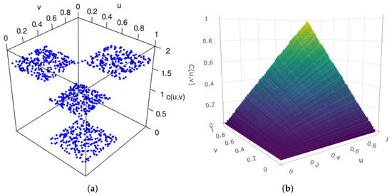
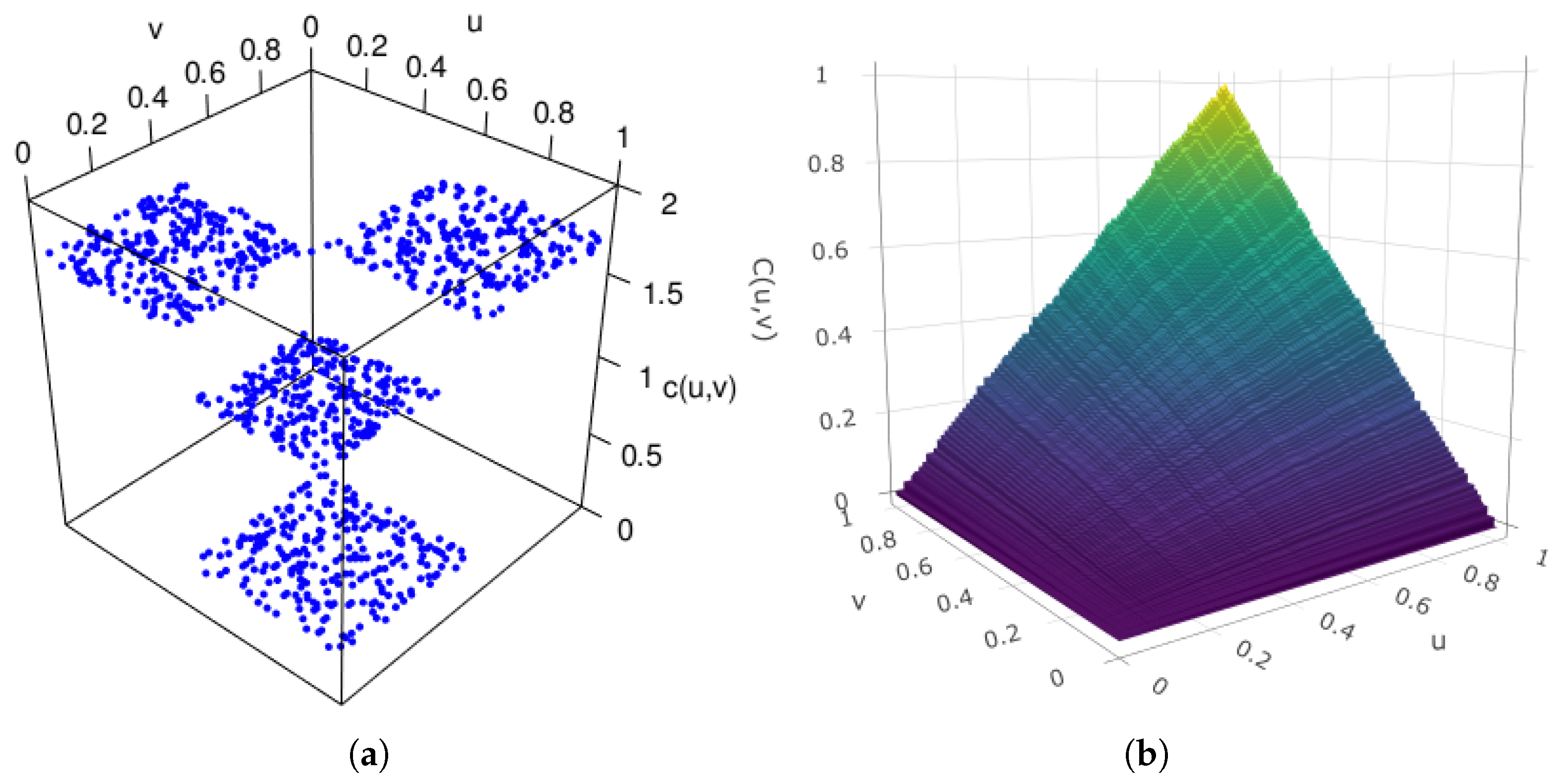
Moreover, ${\int }_0^1{\phi }_j\left(x\right)dx={\int }_0^1{\phi }_j^2\left(x\right)dx-1=0$ and for $j\ne l$, ${\int }_0^1{\phi }_j\left(x\right){\phi }_l\left(x\right)dx=0$. Copula (4) is part of the copulas introduced by Longla [5], known as the Type-I Longla copulas. It is important to note that the functions in (5) are eigen functions of the operator that the copula induces on $L^2(0,1)$, associated with ${\lambda }_j$. They have disjoint supports. These facts play a very important role in the study of the estimation method we are discussing.

For $k=1$, Formula (4) gives

$$\begin{array}{cc}\hfill C_1(u,v)& =uv+\lambda \left[uI\right(0\le u\le 0.5)-(u-1\left)I\right(0.5<u\le 1\left)\right]\hfill \\ \hfill & \left[uI\right(0\le u\le 0.5)-(u-1\left)I\right(0.5<u\le 1\left)\right],\hfill \end{array}$$

(6)

with $\left|\lambda \right|\le 1$. Copula (6) can also be written as

$$C_1(u,v)=uv+\lambda {(1-u)}^{1-\delta \left(u\right)}{u}^{\delta \left(u\right)}{(1-v)}^{1-\delta \left(v\right)}{v}^{\delta \left(v\right)},\mathrm{where}\delta \left(x\right)=I(x<0.5).$$

The copula density and graphs of this copula are given in Table 1 and Figure 1, respectively.

Table 1. Density copula of $C_1(u,v)$.

	${\mathit{u}}_{\mathit{i}-1}\le 0.5$	${\mathit{u}}_{\mathit{i}-1}>0.5$
$u_i>0.5$	$1-\lambda$	$1+\lambda$
$u_i\le 0.5$	$1+\lambda$	$1-\lambda$

Figure 1. (a) Plot of $c_1(u,v)$ and (b) surface plot of $C_1(u,v)$.

For $k=2$, the copula (4) gives

$$\begin{array}{c}\hfill C_2(u,v)=uv+2{\lambda }_0[uI(u\le {\displaystyle \frac{1}{4}})-(u-{\displaystyle \frac{1}{2}})I(u>{\displaystyle \frac{1}{4}})][vI(v\le {\displaystyle \frac{1}{4}})-(v-{\displaystyle \frac{1}{2}})I(v>{\displaystyle \frac{1}{4}})]I(0\le u,v\le {\displaystyle \frac{1}{2}})\\ \hfill +2{\lambda }_1[(u-{\displaystyle \frac{1}{2}})I(u\le {\displaystyle \frac{3}{4}})-(u-1)I(u>{\displaystyle \frac{3}{4}})][(v-{\displaystyle \frac{1}{2}})I(v\le {\displaystyle \frac{3}{4}})-(v-1)I(v>{\displaystyle \frac{3}{4}})]I({\displaystyle \frac{1}{2}}<u,v\le 1),\end{array}$$

(7)

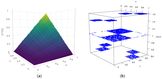
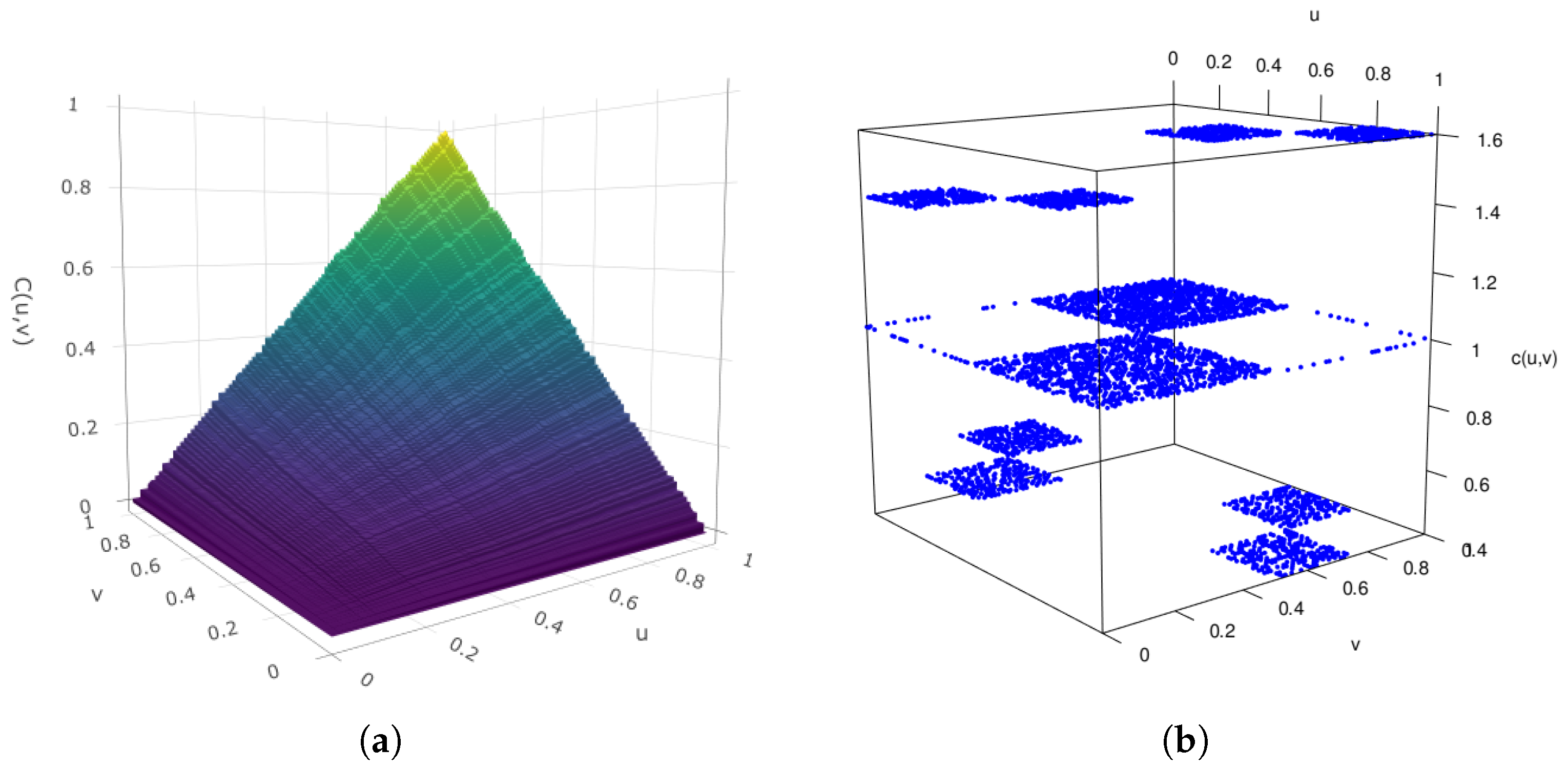
with $|{\lambda }_i|\le {\displaystyle \frac{1}{2}}$. The copula density and graphs of this copula are given in Table 2 and Figure 2, respectively.

Table 2. Density copula of $C_2(u,v)$.

	$0\le \mathit{u}\le 0.25$	$0.25<{\mathit{u}}_{\mathit{i}}\le 0.5$	$0.5<\mathit{u}\le 0.75$	$0.75<\mathit{u}\le 1$
$0.75<u_{i-1}\le 1$	1	1	$1-2{\lambda }_1$	$1+2{\lambda }_1$
$0.5<u_{i-1}\le 0.75$	1	1	$1+2{\lambda }_1$	$1-2{\lambda }_1$
$0.25<u_{i-1}\le 0.5$	$1-2{\lambda }_0$	$1+2{\lambda }_0$	1	1
$0\le u_{i-1}\le 0.25$	$1+2{\lambda }_0$	$1-2{\lambda }_0$	1	1

Figure 2. (a) Surface plot $C_2(u,v)$ and (b) plot of $c_2(u,v)$, both with ${\lambda }_1=0.2$ and ${\lambda }_2=0.3$.

3. Parameter Estimation Methods and Other Results

In this section, we discuss the three different estimation methods used for parameter estimation for stationary Markov chains. We assume that our Markov chains are based on copula (4) and have the uniform distribution on $[0,1]$ as marginals. We use EEF; the estimation method defined by Longla and Hamadou [31], the MLE, and the RE; as constructed by Longla and Peligrad [30]. We establish asymptotic normality of the estimators and construct related confidence intervals and regions. The test statistics for hypothesis testing for the test of independence are provided.

3.1. Estimation Using Eigen Functions (EEF)

Let $U_0,\dots ,U_n$ be a Markov chain with copula (4) and uniform distribution on $[0,1]$ which also serves as the stationary distribution. We consider the following estimators.

$$\begin{array}{cc}\hfill {\widehat{\lambda }}_j& ={\displaystyle \frac{k}{n}}\sum _{i=1}^n\left[I\left(u_i\le {\displaystyle \frac{2j+1}{2k}}\right)-I\left(u_i>{\displaystyle \frac{2j+1}{2k}}\right)\right]\hfill \\ \hfill & \left[I\left(u_{i-1}\le {\displaystyle \frac{2j+1}{2k}}\right)-I\left(u_{i-1}>{\displaystyle \frac{2j+1}{2k}}\right)\right]I_j\left(u_i\right)I_j\left(u_{i-1}\right),\hfill \end{array}$$

(8)

for $j=0,\dots ,k-1$. The EEF are an unbiased and consistent estimator of ${\lambda }_j$. The CLT for ${\widehat{\mathsf{\Lambda }}}^T=({\widehat{\lambda }}_0,\dots ,{\widehat{\lambda }}_{k-1})$ is obtained using results of Longla and Hamadou [31].

Theorem 1. 

For any stationary Markov chain $U_0,\dots ,U_n$ based on the copula (4) and the uniform $(0,1)$ marginal distribution, for the vector ${\mathsf{\Lambda }}^T=({\lambda }_0,\dots ,{\lambda }_{k-1})$, $\sqrt{n}({\widehat{\mathsf{\Lambda }}}^{eef}-\mathsf{\Lambda })\to N(0,\mathsf{\Sigma })$, where Σ is the symmetric positive definite covariance matrix given by

$$\begin{array}{cc}\hfill {\mathsf{\Sigma }}_{j\ell }& =\left\{\begin{array}{cc}1+(2k-3){\lambda }_i^2\hfill & ,\mathrm{when}j=\ell \hfill \\ -3{\lambda }_j{\lambda }_{\ell }\hfill & ,\mathrm{when}j\ne \ell .\hfill \end{array}\right.\hfill \end{array}$$

(9)

See the Appendix A.1 for the proof of Theorem 1.

Confidence regions/intervals for the parameters are given the following corollary.

Corollary 1. 

Let $U_0,\dots ,U_n$ be a stationary Markov chain based on the copula (4) and the uniform $(0,1)$ distribution then for $0<\alpha <1$, the $(1-\alpha )100\%$ confidence interval of each ${\lambda }_j$ is

$$\left({\widehat{\lambda }}_j-z_{{\displaystyle \frac{\alpha }{2}}}{\left[{\displaystyle \frac{1+(2k-3){\widehat{\lambda }}_j^2}{n}}\right]}^{{\displaystyle \frac{1}{2}}},{\widehat{\lambda }}_j+z_{{\displaystyle \frac{\alpha }{2}}}{\left[{\displaystyle \frac{1+(2k-3){\widehat{\lambda }}_j^2}{n}}\right]}^{{\displaystyle \frac{1}{2}}}\right),$$

such that $P(z>z_{\alpha /2})=\alpha /2$ where $z\sim N(0,1)$. Furthermore, for vector Λ, the $(1-\alpha )100\%$ confidence region consists of all the points that satisfy the following:

$$\left\{\mathsf{\Lambda }\in {\left[{\displaystyle \frac{-1}{k}},{\displaystyle \frac{1}{k}}\right]}^k:{(\widehat{\mathsf{\Lambda }}-\mathsf{\Lambda })}^T{\widehat{\mathsf{\Sigma }}}^{-1}(\widehat{\mathsf{\Lambda }}-\mathsf{\Lambda })<{\chi }_{\alpha }^2\left(k\right)\right\},$$

such that $P(X<{\chi }_{\alpha }^2\left(k\right))=1-\alpha$ where $X\sim {\chi }^2\left(k\right)$.

See the Appendix A.2 for the proof of Corollary 1.

3.2. Estimation Using Maximum Likelihood Estimation

Let $U_0,\dots ,U_n$ be a stationary Markov chain with a copula of consecutive states given by (4) and the uniform distribution on $[0,1]$ as its marginal. Based on the definition of ${\phi }_j\left(x\right)$, each of the intervals of $I_j$ splits into two sub-intervals. Let $\mathcal{E}={\left\{{\mathcal{E}}_p\right\}}_{p=0}^{2(k-1)}$ be the set of those sub-intervals, where each ${\mathcal{E}}_{2j}=({\displaystyle \frac{j}{k}},{\displaystyle \frac{2j+1}{2k}}]$ and ${\mathcal{E}}_{2j+1}=({\displaystyle \frac{2j+1}{2k}},{\displaystyle \frac{j+1}{k}}]$ for $j=1,\dots ,k-1$. See that for $j=0$, ${\mathcal{E}}_0=[0,{\displaystyle \frac{1}{2k}}]$ and ${\mathcal{E}}_1=({\displaystyle \frac{1}{2k}},{\displaystyle \frac{1}{k}}]$. Now we define the notation $n_{j\ell }$ which is

$$n_{j\ell }=\sum _{i=1}^{n}I(U_i\in {\mathcal{E}}_j,U_{i-1}\in {\mathcal{E}}_{\ell }).$$

(10)

Using the above the notation we get the likelihood function as

$$\begin{array}{c}\hfill L(\mathbb{U};\lambda )=\prod _{i=1}^{n}c(U_{i-1},U_i)=\prod _{j=0}^{k-1}{(1+k{\lambda }_j)}^{n_{\left(2j\right)\left(2j\right)}+n_{(2j+1)(2j+1)}}{(1-k{\lambda }_j)}^{n_{\left(2j\right)(2j+1)}+n_{(2j+1)\left(2j\right)}}.\end{array}$$

(11)

where $c(u,v)$ is the density copula and is given by

$$c(u,v)=1+\sum _{j=0}^{k-1}{\lambda }_j{\phi }_j\left(u_{i-1}\right){\phi }_j\left(u_i\right).$$

Thus, the MLE obtained by equating the first derivative of (11) to 0 is

$$\begin{array}{cc}\hfill {\widehat{\lambda }}_j^{mle}& ={\displaystyle \frac{n_{\left(2j\right)\left(2j\right)}+n_{(2j+1)(2j+1)}-n_{\left(2j\right)(2j+1)}-n_{(2j+1)\left(2j\right)}}{k(n_{\left(2j\right)\left(2j\right)}+n_{(2j+1)(2j+1)}+n_{\left(2j\right)(2j+1)}+n_{(2j+1)\left(2j\right)})}}.\hfill \end{array}$$

(12)

Remark 1. 

When $k=1$ in (4), the MLE of ${\lambda }_j$ is the same as the EEF of ${\lambda }_j$ obtained in Section 3.1.

We use Billingsley [17] to establish the asymptotic distribution of MLE. We demonstrate the existence and uniqueness of these estimators when the real parameters fall within the support region. Billingsley’s theorem establishes that subject to specific regularity conditions, the MLEs tend towards a normal distribution asymptotically, with variance derived from a variant of Fisher information. The following regularity conditions are satisfied and guaranty asymptotic normality of the MLE.

C1

The Markov chain is ergodic;

C2

The values of v for which $c(u,v)>0$ and $u\in [0,1]$ is independent of $\mathsf{\Lambda }$;

C3

For any $\xi$ and $\mathbb{A}$, $g(\xi ,\mathbb{A};\lambda )=logf(\xi ,\mathbb{A};\lambda )$ where $f(\xi ,\mathbb{A};\lambda )>0$ is the likelihood function, is well defined and the partial derivatives of $f(\xi ,\mathbb{A};\lambda )$ and $g(\xi ,\mathbb{A};\lambda )$ with respect to $\lambda$ exists. Then, for any neighbourhood n of $\lambda$,

$${\int }_X\underset{{\lambda }^{\prime }\in n}{sup}|f_i(\xi ,\mathbb{A};{\lambda }^{\prime })|\mu \left(d\mathbb{A}\right),{\int }_X\underset{{\lambda }^{\prime }\in n}{sup}|f_{ij}(\xi ,\mathbb{A};{\lambda }^{\prime })|\mu \left(d\mathbb{A}\right)\mathrm{and}{E}_{\lambda }\{\underset{{\lambda }^{\prime }\in n}{sup}|g_{ijk}(\xi ,\mathbb{A};{\lambda }^{\prime })|\mu \left(d\mathbb{A}\right)\}$$

are all finite;

C4

For $i,j,k=1,2,\dots ,r$, the Fisher information for each ${\lambda }_i$ is finite and if ${\sigma }_{ij}\left(\lambda \right)=E_{\lambda }({\displaystyle \frac{\partial }{\partial {\lambda }_i}}l(\mathbb{X},\lambda )\times {\displaystyle \frac{\partial }{\partial {\lambda }_j}}l(\mathbb{X},\lambda ))$, then the $r\times r$ matrix ${\sigma }_{ij}\left(\lambda \right)$ is non-singular;

C5

For all $\lambda \in \mathsf{\Lambda }$, the stationary distribution, which exists and is unique, satisfies, $p_{\lambda }(\xi ,·)<<p_{\lambda }(·)$ and for some $\delta >0$, $E_{\lambda }\left(\right|g_i(x_1,x_2;\lambda ){|}^{2+\delta })<\infty .$

The Markov chain generated by the copula (4) satisfies the conditions C1–C5. Thus, by Billingsley [17], the following theorem holds.

Theorem 2. 

For any Markov chain $U_0,\dots ,U_n$ generated by the copula (4) and the uniform $(0,1)$ distribution, for the vector ${\mathsf{\Lambda }}^T=({\lambda }_0,\dots ,{\lambda }_{k-1})$, $\sqrt{n}({\widehat{\mathsf{\Lambda }}}^{mle}-\mathsf{\Lambda })\to (0,\mathsf{\Sigma })$, where

$$\begin{array}{cc}\hfill {\mathsf{\Sigma }}_{j\ell }& =\left\{\begin{array}{cc}1-{\left(k{\lambda }_j\right)}^2\hfill & ,\mathrm{when}j=\ell \hfill \\ 0\hfill & ,\mathrm{when}j\ne \ell .\hfill \end{array}\right.\hfill \end{array}$$

(13)

See the Appendix A.3 for the proof of Theorem 2.

Following Theorem 2, we get the following corollary for the confidence intervals and regions for the ${\lambda }_j$ and $\mathsf{\Lambda }$, respectively.

Corollary 2. 

Let $U_0,\dots ,U_n$ be a stationary Markov chain based on the copula (4) and the uniform distribution on $[0,1]$ and let (12) be the MLE of ${\lambda }_i$. Then, for $0<\alpha <1$, the $(1-\alpha )100\%$ confidence interval of each ${\lambda }_j$ is

$$\left({\widehat{\lambda }}_j^{mle}-z_{{\displaystyle \frac{\alpha }{2}}}{\left[{\displaystyle \frac{1-{\left(k{\widehat{\lambda }}_j^{mle}\right)}^2}{n}}\right]}^{{\displaystyle \frac{1}{2}}},{\widehat{\lambda }}_j^{mle}+z_{{\displaystyle \frac{\alpha }{2}}}{\left[{\displaystyle \frac{1-{\left(k{\widehat{\lambda }}_j^{mle}\right)}^2}{n}}\right]}^{{\displaystyle \frac{1}{2}}}\right).$$

For the vector Λ the $(1-\alpha )100\%$ confidence region is given by

$$\left\{\mathsf{\Lambda }\in {\left[{\displaystyle \frac{-1}{k}},{\displaystyle \frac{1}{k}}\right]}^k:\sum _{j=0}^{k-1}{\displaystyle \frac{n{({\widehat{\lambda }}_j^{mle}-{\lambda }_j)}^2}{1-{\left(k{\widehat{\lambda }}_j^{mle}\right)}^2}}<{\chi }_{\alpha }^2\left(k\right)\right\},$$

where $P(X<{\chi }_{\alpha }^2\left(k\right))=1-\alpha$, $X\sim {\chi }^2\left(k\right)$.

See the Appendix A.4 for the proof of Corollary 2.

3.3. Hypothesis Testing for Independence

It is important to note that, in the copula (4), when the parameters are 0, we achieve independence in the data generated by the copula. The test statistics for the test of independence using the Maximum Likelihood Estimator is given in the following theorem.

Theorem 3. 

For any Markov chain generated by the copula (4) and the uniform distribution on $[0,1]$ as marginals, the test statistics under the null hypothesis, $H_0:{\lambda }_0=\cdots ={\lambda }_{k-1}=0$, is given by ${\displaystyle {\chi }^2=\sum _{j=0}^{k-1}\frac{n{\left({\widehat{\lambda }}_j^{mle}\right)}^2}{1-{\left(k{\widehat{\lambda }}_j^{mle}\right)}^2}}$ and has approximately a chi-square distribution with degrees of freedom k as $n\to \infty$.

3.4. Estimation Using Robust Estimation

Robust estimators have been used in the literature to find unbiased estimators that are not influenced by any discrepancies like outliers. This is especially the case when the data involve a stochastic process, such as a Markov chain, and their density function or the dependence structures are unknown. For our work, we use the method introduced by Longla and Peligrad [30]. They proposed a robust estimator for the mean of a sample of dependent observations. They also developed estimators for ergodic stochastic processes with long memory and finite second moments whose dependence structure is not known or when the density function is unknown. The kernel K and bandwidth $h_n$ needed for the estimator must satisfy the following conditions:

C8

The kernel should be a symmetric bounded density function.

C9

The bandwidth should satisfy $h_n\to 0$ and $n{h}_n\to \infty$ as $n\to \infty$.

C10

For the sequence ${\left\{U_i\right\}}_{i\in \mathbb{N}}$, $\sqrt{n{h}_n}({\overline{U}}_n-{\mu }_U)$ should converge to 0 in probability.

The following result is obtained by using the work of Longla and Peligrad [30] and gives the asymptotic normality and the confidence interval for the robust estimator for individual ${\lambda }_j$. Their estimator is

$${\widehat{\lambda }}_j^{re}={\displaystyle \frac{1}{n{h}_n}}\sum _{i=1}^n{Y}_{ij}exp(-0.5{\left({\displaystyle \frac{X_i}{{\widehat{h}}_n}}\right)}^2).$$

Theorem 4. 

For a stationary Markov chain $U_0,\dots ,U_n$ based on the copula (4) and the uniform $(0,1)$ distribution, ${\displaystyle \sqrt{\frac{n{h}_n}{\overline{Y_{ij}^2}}}({\widehat{\lambda }}_j^{re}\sqrt{1+h_n^2}-{\lambda }_j)\to N\left(0,\frac{1}{\sqrt{2}}\right)}$. Furthermore, for $0<\alpha <1$, the $(1-\alpha )100\%$ confidence intervals for $j=0,\dots ,k-1$ are given by

$$\left({\widehat{\lambda }}_j^{re}\left(\sqrt{1+h_n^2}\right)-z_{\alpha /2}{\left[{\displaystyle \frac{\overline{Y_{ij}^2}}{n{h}_n\sqrt{2}}}\right]}^{1/2},{\widehat{\lambda }}_j^{re}\left(\sqrt{1+h_n^2}\right)+z_{\alpha /2}{\left[{\displaystyle \frac{\overline{Y_{ij}^2}}{n{h}_n\sqrt{2}}}\right]}^{1/2}\right).$$

Remark 2. 

Note that $Y_{ij}={\phi }_j\left(u_i\right){\phi }_j\left(u_{i-1}\right)$, and since the expected value of $Y_{ij}$ can be estimated as average of $Y_{ij}$, which is the EEF given in Theorem 1, that is, $\widehat{E}\left(Y_{ij}\right)={\widehat{\lambda }}_j$. Similarly, the expected value of $Y_{ij}^2$ is estimated as

$$\widehat{E}\left(Y_{ij}^2\right)=E\left({\phi }_j{\left(u_i\right)}^2{\phi }_j{\left(u_{i-1}\right)}^2\right)=1+\sum _{z=1}^{m-1}{\widehat{\lambda }}_z{\left({\int }_0^1{\phi }_z\left(x\right){\phi }_j^2\left(x\right)dx\right)}^2=1.$$

The above expression of $E\left({\phi }_j{\left(u_i\right)}^2{\phi }_j{\left(u_{i-1}\right)}^2\right)$ is taken from Longla and Hamadou [31] and is calculated as shown in the proof of Theorem 1. For our choice of X and kernel, the optimal bandwidth is given as $h_n={\left[{\displaystyle \frac{E\left(Y^2\right)}{\sqrt{2}n{\left(EY\right)}^2}}\right]}^{1/5}$ and the estimator is ${\widehat{h}}_n={\left[{\displaystyle \frac{1}{\sqrt{2}n{\widehat{\lambda }}_j^2}}\right]}^{1/5}$. Thus, the robust estimator of ${\lambda }_j$ is now given by

$${\widehat{\lambda }}_j^{rewl}={\displaystyle \frac{1}{n{\widehat{h}}_n}}\sum _{i=1}^n{Y}_{ij}exp(-0.5{\left({\displaystyle \frac{X_i}{{\widehat{h}}_n}}\right)}^2)$$

and the confidence intervals are

$$\left({\widehat{\lambda }}_j^{rewl}\left(\sqrt{1+{\widehat{h}}_n^2}\right)-z_{\alpha /2}{\left[{\displaystyle \frac{1}{n{\widehat{h}}_n\sqrt{2}}}\right]}^{1/2},{\widehat{\lambda }}_j^{rewl}\left(\sqrt{1+{\widehat{h}}_n^2}\right)+z_{\alpha /2}{\left[{\displaystyle \frac{1}{n{\widehat{h}}_n\sqrt{2}}}\right]}^{1/2}\right).$$

3.5. Measures of Association and Their Estimators

We use the Formulas (2) and (3) to obtain the following expressions:

$${\rho }_S={\displaystyle \frac{3}{4k^3}}\sum _{j=0}^{k-1}{\lambda }_j\mathrm{and}\tau ={\displaystyle \frac{1}{2k^3}}\sum _{j=0}^{k-1}{\lambda }_j.$$

(14)

To obtain the estimator of the measures of associations, we plug in the MLE ${\widehat{\lambda }}_j$ in the place of ${\lambda }_j$, which gives us

$${\widehat{\rho }}_S={\displaystyle \frac{3}{4k^3}}\sum _{j=0}^{k-1}{\widehat{\lambda }}_j^{mle}\mathrm{and}\widehat{\tau }={\displaystyle \frac{1}{2k^3}}\sum _{j=0}^{k-1}{\widehat{\lambda }}_j^{mle}.$$

(15)

Theorem 5. 

For a stationary Markov chain $U_0,\dots ,U_n$ generated by the copula (4) and the uniform $(0,1)$ distribution, $\sqrt{n}({\widehat{\rho }}_S-{\rho }_S)\to N(0,{\sigma }_{{\rho }_S}^2),$ where ${\displaystyle {\sigma }_{{\rho }_S}^2=\frac{9}{16k^3}(1-k\sum _{j=0}^{k-1}\left({\lambda }_j^2\right))}$. For $0\le \alpha \le 1$, the $100(1-\alpha )\%$ confidence interval for ${\rho }_S$ is given by ${\displaystyle {\widehat{\rho }}_S\pm z_{\frac{\alpha }{2}}{\sigma }_{{\widehat{\rho }}_S}^2}$, where ${\sigma }_{{\widehat{\rho }}_S}^2$ is the estimate of ${\sigma }_{{\rho }_S}^2$ obtained by replacing ${\lambda }_j$ by their MLEs.

For the copula (4), ${\rho }_S={\displaystyle \frac{3}{2}}\tau$, thus the estimator, the asymptotic normality, and the $(1-\alpha )100\%$ confidence interval of $\tau$ follows from Theorem 5.

Nelsen [2], Joe [11], Durante, and Sempi [32] and many more have discussed the use of these measures of association to estimate the parameters of copula models. The method of estimations using measures of association does not work for copula (4) because ${\rho }_s=\tau =0$ may be true even when ${\lambda }_j$ are not 0. This is due to the presence of the sum of ${\lambda }_j$ in the expression of ${\rho }_s$ and $\tau$, which can be zero for non-zero ${\lambda }_j$. It can also be noted that, in our copula models, the data are independent if, and only if, ${\lambda }_j$ is 0. For example, for $k=2$, if ${\lambda }_0=-0.1$ and ${\lambda }_1=0.1$, then we get ${\rho }_s=\tau =0$, but the data have dependence. Thus, measures of association can not be used to estimate parameters of the copula (4), directing us to use different methods of estimation, which are discussed in this paper despite it being a robust method of estimation in other cases.

4. Examples and Simulations

We have provided four estimators of copula parameters in each of the cases, along with related asymptotic results.

For the simulations, we first generated the Markov chains from each of the copulas using the following steps:

• Generate two uniform variables $U_1$ and $T_t$ for all $t=1,\dots ,n$, which are independent of each other.
• Next, for each $t=2,\dots ,n$ we equate $T_t$ to the partial derivative of the copula with respect to u and solve for v, the expression for v obtained forms the next variable $U_t$ of the Markov chain.
• Repeat the above step for $t=2,\dots ,n$. The sequence ${\left\{U_t\right\}}_{t=0}^n$ forms the desired Markov chain and is said to be generated by the copula with a specific $\lambda$.

We generate Markov chains of three different sizes: n = 25,000, 50,000, and 75,000. We report coverage probabilities (CPs), confidence intervals mean lengths (CIMLs), and the joint coverage probabilities (in the case of two-parameter perturbation).

4.1. One Parameter Perturbation

The one parameter pertubation of copula (4) is copula (6), as discussed in Section 2. Since we only have one parameter, all calculations become very straightforward. All the estimators for the copula (6) are given below:

• The Estimator using Eigen Functions (EEF) of $\lambda$ is same as the MLE and is given by (16):

  $$\widehat{\lambda }={\displaystyle \frac{1}{n}}\sum _{i=1}^n(2I(0\le U_i\le 0.5)-1)(2I(0\le U_{i-1}\le 0.5)-1).$$

  (16)
  The CLT for the above estimator for $\lambda$ is $\sqrt{n}(\widehat{\lambda }-\lambda )\to N(0,1-{\lambda }^2)$ and the $(1-\alpha )100\%$ confidence interval is $(\widehat{\lambda }-z_{{\displaystyle \frac{\alpha }{2}}}{\left({\displaystyle \frac{1-{\widehat{\lambda }}^2}{n}}\right)}^{1/2},\widehat{\lambda }+z_{{\displaystyle \frac{\alpha }{2}}}{\left({\displaystyle \frac{1-{\widehat{\lambda }}^2}{n}}\right)}^{1/2})$.
• The expression of the robust estimator and the robust estimator with ${\widehat{\lambda }}_j$ is the same as in Section 3.4.

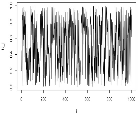
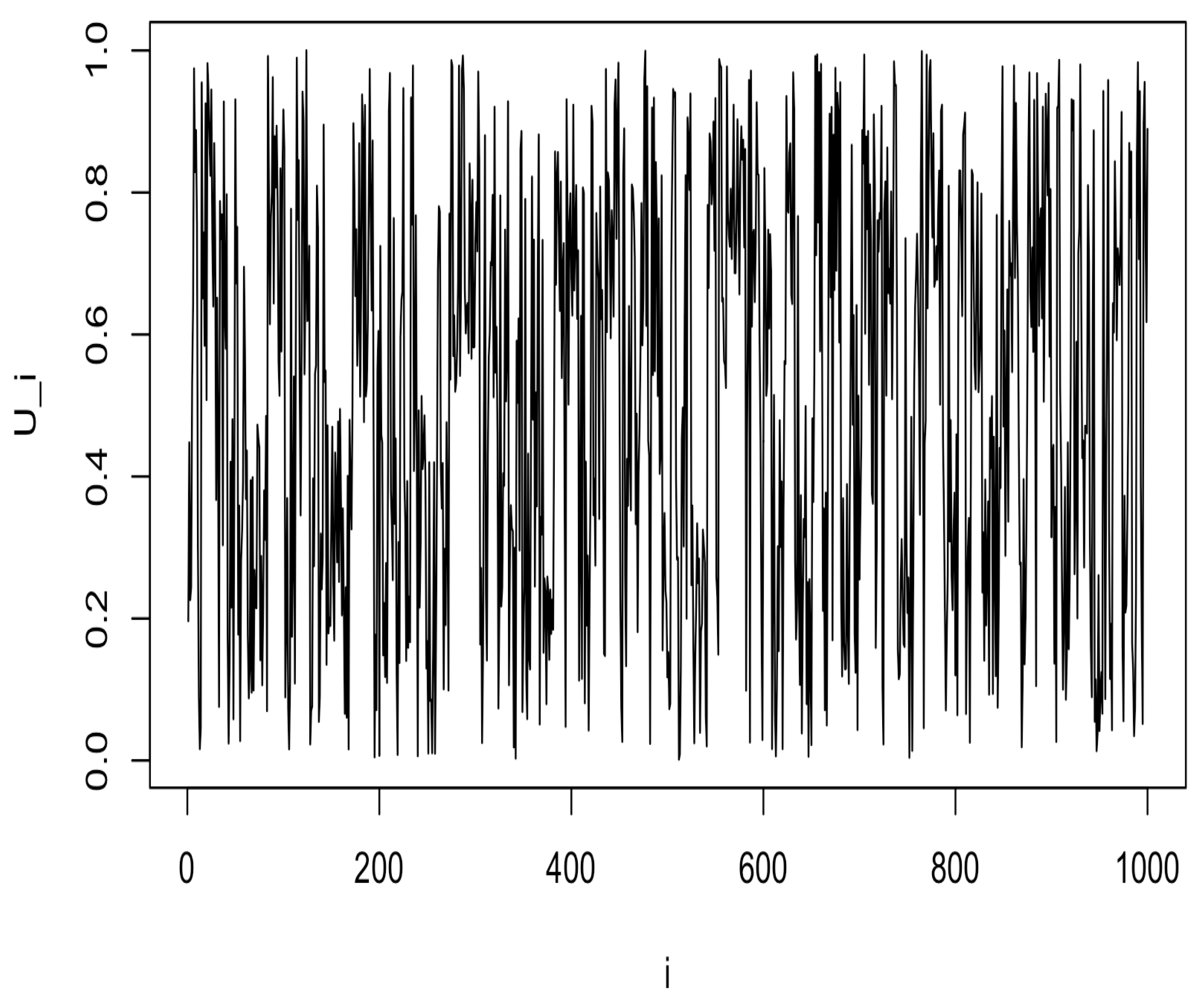
We generate the Markov chain following the steps at the beginning of Section 4. The Markov chain generated by this copula for $n=1000$ and $\lambda =0.6$ is shown in Figure 3. Table 3, Table 4 and Table 5 contain the EEF and RE of $\lambda$ for the following values: $\lambda =0.2,-0.5$, and $0.7$. We report the EEF only since MLE is the same as EEF in one parameter case.

Figure 3. Time series plot of the Markov chain generated by copula 1 with $n=1000$ and $\lambda =0.6$.

Table 3. Estimated values from simulation with $\lambda =0.2$.

$\mathit{\lambda }=0.2$
Estimators	n= 25,000		n= 50,000		n= 75,000
	CP	CIML	CP	CIML	CP	CIML
$\widehat{\lambda }$	93	0.019	94	0.017	95	0.014
${\widehat{\lambda }}^{re}$	89	0.049	90	0.047	91	0.043

Table 4. Estimated values from simulation with $\lambda =-0.5$.

$\mathit{\lambda }=-0.5$
Estimators	n= 25,000		n= 50,000		n= 75,000
	CP	CIML	CP	CIML	CP	CIML
$\widehat{\lambda }$	94	0.018	94	0.016	95	0.013
${\widehat{\lambda }}^{re}$	90	0.050	91	0.045	92	0.043

Table 5. Estimated values from simulation with $\lambda =0.7$.

$\mathit{\lambda }=0.7$
Estimators	n= 25,000		n= 50,000		n= 75,000
	CP	CIML	CP	CIML	CP	CIML
$\widehat{\lambda }$	94	0.019	95	0.017	95	0.014
${\widehat{\lambda }}^{re}$	89	0.055	90	0.049	90	0.045

For the test statistics for the hypothesis testing under the null hypothesis, $H_0:\lambda =0$, the test statistics is given as ${\chi }^2={\displaystyle \frac{n{\left({\widehat{\lambda }}^{mle}\right)}^2}{1-{\left({\widehat{\lambda }}^{mle}\right)}^2}}$; this approximately follows a chi-square distribution with 1 degree of freedom. We simulated a Markov chain based on copula (6), where the parameter was $\lambda =0$. A test for the hypothesis $H_0:\lambda =0$ against $H_{\alpha }:\lambda \ne 0$ was performed. The results of the hypothesis testing are listed in Table 6; based on the results, we fail to reject the null hypothesis.

Table 6. Test for the assumption of independence.

n = 10,000, $\mathit{\alpha }$ = 0.05
Using copula 1	test statistics	p-value
	1.2953	0.8651

The Spearman’s Rho for this copula is ${\rho }_S={\displaystyle \frac{3}{4}}\lambda$ and it is estimator obtained using the MLE is

$${\widehat{\rho }}_S={\displaystyle \frac{3}{4}}\widehat{\lambda }={\displaystyle \frac{3}{4}}(2\left({\displaystyle \frac{n_{11}+n_{22}}{n}}\right)-1).$$

The CLT is

$$\sqrt{n}({\widehat{\rho }}_S-{\rho }_S)\to N(0,{\displaystyle \frac{9}{16}}(1-{\lambda }^2))$$

and the $100(1-\alpha )\%$ confidence interval is given by $({\widehat{\rho }}_S-z_{{\displaystyle \frac{\alpha }{2}}}\sigma \left({\widehat{\rho }}_S\right),{\widehat{\rho }}_S+z_{{\displaystyle \frac{\alpha }{2}}}\sigma \left({\widehat{\rho }}_S\right))$. The results regarding Kendall’s Tau can be easily obtained from those of Spearman’s rho.

4.2. Two Parameter Perturbation

For the case $k=2$, we have two intervals (or $I_j$): $[0,{\displaystyle \frac{1}{2}}]$ and $({\displaystyle \frac{1}{2}},1]$. All the estimators for this copula are given below:

• The Estimator using Eigen Functions (EEF) of ${\lambda }_j$ is given by

  $$\begin{array}{cc}\hfill {\widehat{\lambda }}_j& ={\displaystyle \frac{2}{n}}\sum _{i=1}^n\left(I\left(u_i\le {\displaystyle \frac{2j+1}{4}}\right)-I\left(u_i>{\displaystyle \frac{2j+1}{4}}\right)\right)I_j\left(u_i\right)\hfill \\ \hfill & \left(I\left(u_{i-1}\le {\displaystyle \frac{2j+1}{4}}\right)-I\left(u_{i-1}>{\displaystyle \frac{2j+1}{4}}\right)\right)I_j\left(u_{i-1}\right),\hfill \end{array}$$

  for $j=0,1$. The CLT for the individual estimators is $\sqrt{n}(\widehat{\lambda }-\lambda )\to N(0,1+{\lambda }_i^2)$ and $\sqrt{n}(\widehat{\mathsf{\Lambda }}-\mathsf{\Lambda })\to N(0,\mathsf{\Sigma }),$ for the vector $\widehat{\mathsf{\Lambda }}={({\widehat{\lambda }}_0,{\widehat{\lambda }}_1)}^T$ where $\mathsf{\Sigma }=\left(\begin{array}{cc}1+{\lambda }_0^2& -3{\lambda }_0{\lambda }_1\\ -3{\lambda }_0{\lambda }_1& 1+{\lambda }_1^2\end{array}\right)$ is the covariance matrix.
  The $(1-\alpha )100\%$ confidence interval for ${\lambda }_j$ is

  $$\left({\widehat{\lambda }}_j-z_{{\displaystyle \frac{\alpha }{2}}}{\left({\displaystyle \frac{1+{\widehat{\lambda }}_j^2}{n}}\right)}^{{\displaystyle \frac{1}{2}}},{\widehat{\lambda }}_j+z_{{\displaystyle \frac{\alpha }{2}}}{\left({\displaystyle \frac{1+{\widehat{\lambda }}_j^2}{n}}\right)}^{{\displaystyle \frac{1}{2}}}\right).$$
  Furthermore, the $(1-\alpha )100\%$ confidence region for $\widehat{\mathsf{\Lambda }}={({\widehat{\lambda }}_0,{\widehat{\lambda }}_1)}^T$ is given by the ellipse,

  $$n\left({\displaystyle \frac{(1+{\widehat{\lambda }}_1^2){({\widehat{\lambda }}_0-{\lambda }_0)}^2+(1+{\widehat{\lambda }}_0^2){({\widehat{\lambda }}_1-{\lambda }_1)}^2+6{\widehat{\lambda }}_0{\widehat{\lambda }}_1({\widehat{\lambda }}_0-{\lambda }_0)({\widehat{\lambda }}_1-{\lambda }_1)}{(1+{\widehat{\lambda }}_0^2)(1+{\widehat{\lambda }}_1^2)-9{\left({\widehat{\lambda }}_0{\widehat{\lambda }}_1\right)}^2}}\right)<{\chi }_{\left(2\right)}^2.$$
• The MLE is given as

  $${\widehat{\lambda }}_j^{mle}={\displaystyle \frac{n_{\left(j\right)\left(j\right)}+n_{(j+1)(j+1)}-n_{\left(j\right)(j+1)}-n_{(j+1)\left(j\right)}}{2(n_{\left(j\right)\left(j\right)}+n_{(j+1)(j+1)}+n_{\left(j\right)(j+1)}+n_{(j+1)\left(j\right)})}},\mathrm{for}j=0,1.$$
  The asymptotic normality for ${\widehat{\mathsf{\Lambda }}}^{mle}={({\widehat{\lambda }}_0^{mle},{\widehat{\lambda }}_1^{mle})}^T$ is given as $\sqrt{n}({\widehat{\mathsf{\Lambda }}}^{mle}-\mathsf{\Lambda })\to (0,\mathsf{\Sigma })$, where $\mathsf{\Sigma }=\left(\begin{array}{cc}1-4{\lambda }_0^2& 0\\ 0& 1-4{\lambda }_1^2\end{array}\right)$ is the covariance matrix.
  The $(1-\alpha )100\%$ confidence interval the ${\lambda }_i$ is given by

  $$\left({\widehat{\lambda }}_i^{mle}-z_{{\displaystyle \frac{\alpha }{2}}}{\left({\displaystyle \frac{1-4{\left({\widehat{\lambda }}_i^{mle}\right)}^2}{n}}\right)}^{{\displaystyle \frac{1}{2}}},{\widehat{\lambda }}_i^{mle}+z_{{\displaystyle \frac{\alpha }{2}}}{\left({\displaystyle \frac{1-4{\left({\widehat{\lambda }}_i^{mle}\right)}^2}{n}}\right)}^{{\displaystyle \frac{1}{2}}}\right)$$

  where $z_{\alpha /2}$ is the critical value from the standard normal distribution for $0<\alpha <1$ level of significance.
  The confidence region for $\widehat{\mathsf{\Lambda }}$ is given by the rectangle,

  $$n\left({\displaystyle \frac{{({\widehat{\lambda }}_0^{mle}-{\lambda }_0)}^2}{1-4{\left({\widehat{\lambda }}_0^{mle}\right)}^2}}+{\displaystyle \frac{{({\widehat{\lambda }}_1^{mle}-{\lambda }_1)}^2}{1-4{\left({\widehat{\lambda }}_1^{mle}\right)}^2}}\right)<{\chi }_{\left(2\right)}^2.$$
• The expression of the robust estimator and the robust estimator with ${\widehat{\lambda }}_j$ is the same as in Section 3.4.

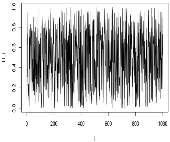
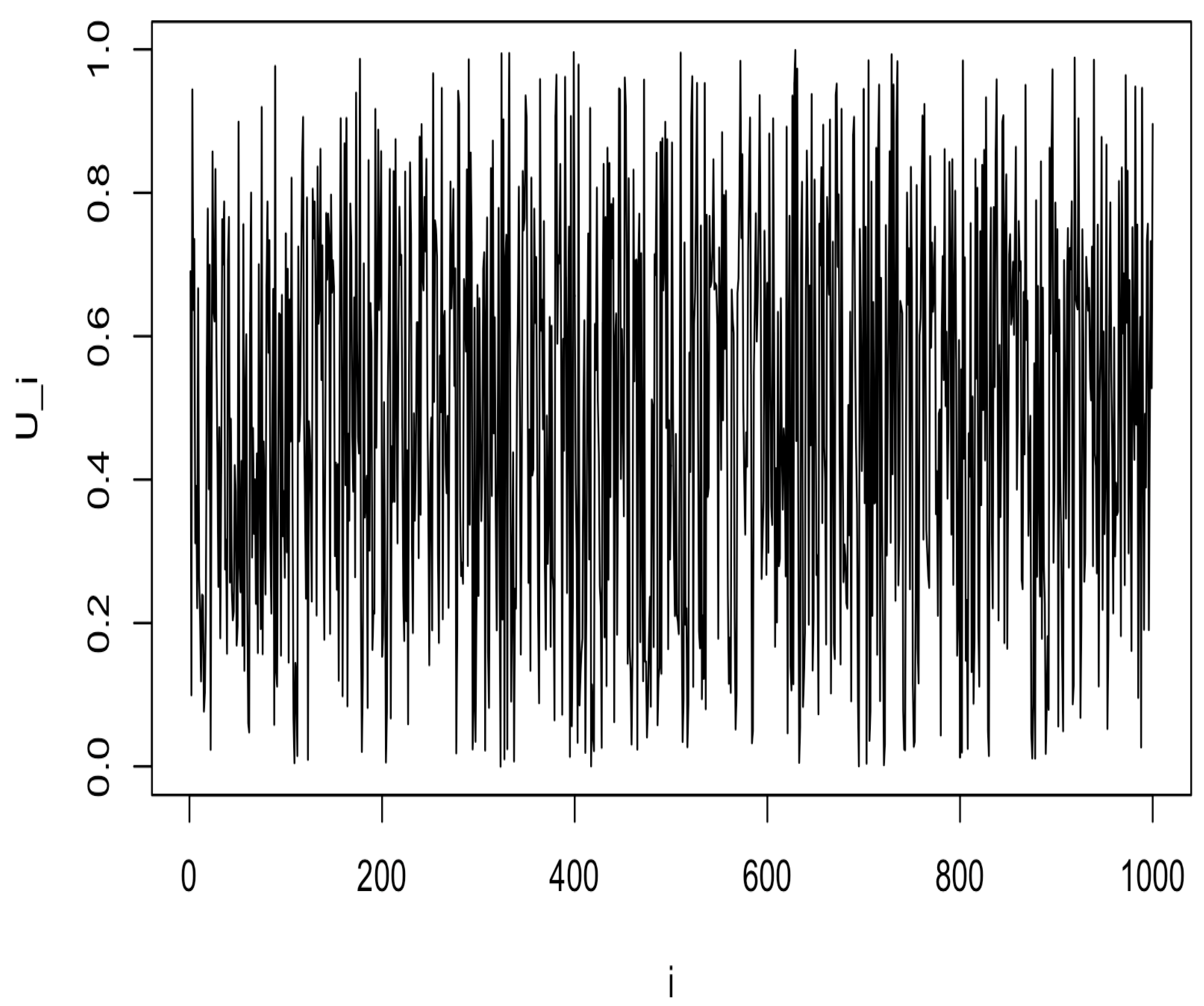
We generate the Markov chain following the steps in Section 4. The Markov chain generated by this copula for $n=1000$ and ${\lambda }_0=0.2$ and ${\lambda }_1=-0.3$ is shown in Figure 4.

Figure 4. Time series plot of the Markov chains with $n=1000$ and ${\lambda }_1=0.2$ and ${\lambda }_2=-0.3$.

Table 7, Table 8 and Table 9 contain the EEF, MLE, and RE of ${\lambda }_j$ for three different combinations: ${\lambda }_0=0.1,{\lambda }_1=0.4$, ${\lambda }_0=-0.2,{\lambda }_1=-0.3$ and ${\lambda }_0=-0.4,{\lambda }_1=0.2$. We do not report the REWL here as well for the same reason as stated in the case of one parameter.

Table 7. Individual coverage probabilities (CPs), confidence interval mean lengths (CIMLs), and joint coverage probabilities (Jnt CPs) for the estimated values from simulation with ${\lambda }_0=-0.2$ and ${\lambda }_1=-0.3$.

${\mathit{\lambda }}_0=0.1$ and ${\mathit{\lambda }}_1=0.4$
Estimators		n= 25,000			n= 50,000			n= 75,000
		CP	CIML	Jnt CP	CP	CIML	Jnt CP	CP	CIML	Jnt CP
$\widehat{\mathsf{\Lambda }}$	${\widehat{\lambda }}_0$	94.2	0.033	93.8	94.8	0.029	94.0	95.0	0.025	94.3
	${\widehat{\lambda }}_1$	96.8	0.032		95.9	0.031		95.1	0.030
${\widehat{\mathsf{\Lambda }}}^{mle}$	${\widehat{\lambda }}_0$	95.4	0.026	92.7	95.2	0.023	93.4	95.0	0.021	93.6
	${\widehat{\lambda }}_1$	95.9	0.021		95.6	0.019		95.2	0.017
${\widehat{\mathsf{\Lambda }}}^{re}$	${\widehat{\lambda }}_0$	90.8	0.037		91.6	0.045		92.9	0.036
	${\widehat{\lambda }}_1$	90.6	0.046		91.8	0.065		92.8	0.051

Table 8. Individual coverage probabilities (CPs), confidence interval mean lengths (CIMLs), and joint coverage probabilities (Jnt CPs) for the estimated values from simulation with ${\lambda }_0=0.1$ and ${\lambda }_1=0.4$.

${\mathit{\lambda }}_0=-0.2$ and ${\mathit{\lambda }}_1=-0.3$
Estimators		n= 25,000			n= 50,000			n= 75,000
		CP	CIML	Jnt CP	CP	CIML	Jnt CP	CP	CIML	Jnt CP
$\widehat{\mathsf{\Lambda }}$	${\widehat{\lambda }}_0$	95.8	0.029	92.2	95.5	0.026	93.4	95.1	0.025	93.8
	${\widehat{\lambda }}_1$	96.5	0.033		95.9	0.031		95.1	0.030
${\widehat{\mathsf{\Lambda }}}^{mle}$	${\widehat{\lambda }}_0$	94.7	0.032	92.9	94.9	0.028	93.1	95.1	0.025	93.5
	${\widehat{\lambda }}_1$	94.9	0.025		95.2	0.021		95.6	0.017
${\widehat{\mathsf{\Lambda }}}^{re}$	${\widehat{\lambda }}_0$	84.8	0.043		85.3	0.039		85.9	0.036
	${\widehat{\lambda }}_1$	83.6	0.056		83.9	0.051		84.5	0.045

Table 9. Individual coverage probabilities (CPs), confidence interval mean lengths (CIMLs), and joint coverage probabilities (Jnt CPs) for the estimated values from simulation with ${\lambda }_0=-0.4$ and ${\lambda }_1=0.2$.

${\mathit{\lambda }}_0=-0.4$ and ${\mathit{\lambda }}_1=0.2$
Estimators		n= 25,000			n= 50,000			n= 75,000
		CP	CIML	Jnt CP	CP	CIML	Jnt CP	CP	CIML	Jnt CP
$\widehat{\mathsf{\Lambda }}$	${\widehat{\lambda }}_0$	93.8	0.027	93.2	94.6	0.026	93.7	94.9	0.021	94.1
	${\widehat{\lambda }}_1$	93.5	0.027		93.9	0.022		94.8	0.020
${\widehat{\mathsf{\Lambda }}}^{mle}$	${\widehat{\lambda }}_0$	94.2	0.024	92.9	94.5	0.020	93.5	95.1	0.015	93.9
	${\widehat{\lambda }}_1$	94.4	0.021		95.0	0.017		95.1	0.014
${\widehat{\mathsf{\Lambda }}}^{re}$	${\widehat{\lambda }}_0$	84.6	0.044		85.4	0.037		85.8	0.031
	${\widehat{\lambda }}_1$	83.9	0.046		84.3	0.041		84.9	0.038

The test statistics for testing the null hypothesis, $H_0:{\lambda }_0={\lambda }_1=0$, is given by ${\chi }^2={\displaystyle \frac{n{({\widehat{\lambda }}_0^{mle}-{\lambda }_0)}^2}{1-4{\left({\widehat{\lambda }}_0^{mle}\right)}^2}}+{\displaystyle \frac{n{({\widehat{\lambda }}_1^{mle}-{\lambda }_1)}^2}{1-4{\left({\widehat{\lambda }}_1^{mle}\right)}^2}}$ and it asymptotically follows a chi-square distribution with 2 degrees of freedom. We simulated a Markov chain generated by the copula (7) where the parameters ${\lambda }_0$ and ${\lambda }_1$ are 0; then, we performed the test described above. The results for the test are listed in Table 10. Based on p-value we fail to reject the null hypothesis.

Table 10. Test for the assumption of independence.

n = 10,000, $\mathit{\alpha }$ = 0.05
Using copula 2	test statistics	p-value
	2.4373	0.5913

Similar to case 1, knowing the Spearman’s Rho $\rho$ is sufficient for us to derive the Kendall’s Tau $\tau$. The Spearman’s Rho for this copula is ${\rho }_S={\displaystyle \frac{3}{32}}({\lambda }_0+{\lambda }_1)$, and its estimator can be obtained using the MLE:

$${\widehat{\rho }}_S={\displaystyle \frac{3}{32}}({\widehat{\lambda }}_0+{\widehat{\lambda }}_1)={\displaystyle \frac{3}{64}}\left(\sum _{j=0}^1{\displaystyle \frac{n_{\left(j\right)\left(j\right)}+n_{(j+1)(j+1)}-n_{\left(j\right)(j+1)}-n_{(j+1)\left(j\right)}}{(n_{\left(j\right)\left(j\right)}+n_{(j+1)(j+1)}+n_{\left(j\right)(j+1)}+n_{(j+1)\left(j\right)})}}\right).$$

The CLT is

$$\sqrt{n}({\widehat{\rho }}_S-{\rho }_S)\to N(0,{\sigma }^2\left({\widehat{\rho }}_S\right)),$$

where ${\sigma }^2\left({\widehat{\rho }}_S\right)={\displaystyle \frac{9}{{64}^2}}(2-4({\lambda }_0^2+{\lambda }_1^2))$ and the $100(1-\alpha )\%$ confidence interval for ${\widehat{rho}}_S$ is given by $({\widehat{\rho }}_S-z_{{\displaystyle \frac{\alpha }{2}}}\sigma \left({\widehat{\rho }}_S\right),{\widehat{\rho }}_S+z_{{\displaystyle \frac{\alpha }{2}}}\sigma \left({\widehat{\rho }}_S\right))$.

Remark 3. 

Following are the conclusion from the simulation study:

• During simulation, we noticed that for increasing n, EEF was the most efficient method of estimation in terms of time-efficiency.
• The EEF is as accurate as MLE, judging based on the CIML, and its CPs start behaving well as n grows. Surprisingly, the MLE underperformed as compared to the EEF in terms of the joint CP.
• The confidence intervals obtained for the parameter using the EEF method and the MLE are narrower compared to the robust estimators.
• The performance of the robust estimator does not improve much by using the EEF, but it performs slightly better than the robust estimator itself.
• The choice/combination of values of ${\lambda }_j$ had no effect on the performances of the estimators or the estimation method used. The EEF performs best irrespective to the values of ${\lambda }_j$s.
• We have not reported the values for the robust estimator with ${\widehat{\lambda }}_j$ since it did not perform any better than the robust estimator itself.

5. Discussion

This paper focuses on stationary Markov chains generated by the copula given by (4) and the uniform distribution on $[0,1]$, which serves as its marginal and stationary distributions. For this copula, the estimation of the copula parameters along with their asymptotic normality is studied for the first time in this paper. Due to the copulas’ orthogonal and orthonormal properties, the deduction of their asymptotic behavior becomes relatively simple. From this work, we can see that the EEF method defined by Longla and Hamadou [31] captures the dependence between the parameters more accurately, and is a comparable estimator to the MLE, but performs much better than the RE. The importance of the EEF method is also seen when we compute expressions for the measures of dependence.

The simulations were carried out for Markov chains generated by the copula given by (6) and (7) for large values of n. The simulation study makes it evident that EEF can be considered a better and efficient estimation method for this family of copula than any other method. Even though MLE is a more common method of estimation, in copulas with non-continuous support, EEF proves to be a better method of estimation.

This work is the beginning of our explorations into the various Markov chains that could be generated using this family of copulas. Future research related to this copula family includes the use of non-uniform marginals that have parametric and non-parametric forms and unknown marginals. This work brings many other questions to light that might not be as straightforward to answer.

Appendix A.1. Proof of Theorem 1

Proof. 

Let $U_0,\dots ,U_n$ be a stationary Markov chain based on the copula (4) and the uniform distribution on $[0,1]$. The EEF of the parameters ${\lambda }_j$ are given by (8). Let $\widehat{\mathsf{\Lambda }}={({\widehat{\lambda }}_0,\dots ,{\widehat{\lambda }}_{k-1})}^T$, then by using Theorem 3.1 from Longla and Hamadou [31] we get the CLT as $\sqrt{n}(\widehat{\mathsf{\Lambda }}-\mathsf{\Lambda })\to N(0,\mathsf{\Sigma })$, where the variance ${\sigma }_j$ (or the diagonal elements) is

$$\begin{array}{cc}\hfill {\sigma }_j^2& =1-{\lambda }_j^2+\sum _{z=0}^1{\lambda }_z{\left({\int }_0^1{\phi }_z\left(x\right){\phi }_j^2\left(x\right)dx\right)}^2+2{\lambda }_j^2({\int }_0^1{\phi }_j^4\left(x\right)dx-1)\hfill \\ \hfill & +2\sum _{m=2}^{\infty }{\lambda }_j^2\sum _{z=0}^1{\lambda }_z^{m-1}{\left({\int }_0^1{\phi }_z\left(x\right){\phi }_j^2\left(x\right)dx\right)}^2\hfill \end{array}$$

(A1)

and the off-diagonal elements of $\mathsf{\Sigma }$ are given by

$$\begin{array}{cc}\hfill {\mathsf{\Sigma }}_{j\ell }& =\underset{n\to \infty }{lim}ncov({\widehat{\lambda }}_j,{\widehat{\lambda }}_{\ell })\hfill \\ \hfill & =cov({\phi }_j\left(U_0\right){\phi }_j\left(U_1\right),{\phi }_{\ell }\left(U_0\right){\phi }_{\ell }\left(U_1\right))+2\sum _{m=1}^{\infty }cov({\phi }_j\left(U_0\right){\phi }_j\left(U_1\right),{\phi }_{\ell }\left(U_m\right){\phi }_{\ell }\left(U_{m+1}\right))\hfill \\ \hfill & =\sum _{z=0}^1{\lambda }_z{\left({\int }_0^1{\phi }_z\left(x\right){\phi }_j\left(x\right){\phi }_{\ell }\left(x\right)dx\right)}^2-{\lambda }_j{\lambda }_{\ell }+2{\lambda }_j{\lambda }_{\ell }({\int }_0^1{\phi }_j^2\left(x\right){\phi }_{\ell }^2\left(x\right)dx-1)\hfill \\ \hfill & +2\sum _{m=2}^{\infty }{\lambda }_j{\lambda }_{\ell }\sum _{z=0}^1{\lambda }_z\left({\int }_0^1{\phi }_z\left(x\right){\phi }_j^2\left(x\right)dx\right)\left({\int }_0^1{\phi }_z\left(x\right){\phi }_{\ell }^2\left(x\right)dx\right)\hfill \end{array}$$

(A2)

For our case, the integrals in (A1) are

$$\begin{array}{cc}\hfill {\int }_j^1{\phi }_z\left(x\right){\phi }_j^2\left(x\right)dx& =\left\{\begin{array}{cc}{\int }_0^1{\phi }_j^3\left(x\right)dx={\int }_{{\displaystyle \frac{2j+1}{2n}}}^{{\displaystyle \frac{j+1}{n}}}{\left(\sqrt{k}\right)}^{3}dx-{\int }_{{\displaystyle \frac{2j+1}{2n}}}^{{\displaystyle \frac{j}{n}}}{\left(\sqrt{k}\right)}^{3}dx=0\hfill & ,z=j\hfill \\ {\int }_0^1{\phi }_z\left(x\right){\phi }_j^2\left(x\right)dx=0\hfill & ,z\ne j,\hfill \end{array}\right.\hfill \end{array}$$

${\int }_0^1{\phi }_j^4\left(x\right)dx={\int }_0^1{k}^{2}dx=k^2\left({\displaystyle \frac{1}{k}}\right)=k$ and ${\int }_0^1{\phi }_j^2\left(x\right){\phi }_{\ell }^2\left(x\right)dx=0$.

Using these integrals, we find that variance ${\sigma }_j^2=1+(2k-3){\lambda }_j^2$ for each ${\lambda }_j$ and the off diagonal elements ${\mathsf{\Sigma }}_{j\ell }$ given in (A2) are ${\mathsf{\Sigma }}_{j\ell }=-3{\lambda }_j{\lambda }_{\ell }$. □

Appendix A.2. Proof of Corollary 1

Proof. 

The confidence intervals for individual ${\lambda }_j$ are obtained by using the standard format of confidence interval, $(\mathrm{point}\mathrm{estimate}\pm \mathrm{critical}\mathrm{value}\times \mathrm{standard}\mathrm{error}\mathrm{of}\mathrm{point}\mathrm{estimate}).$ Since the point estimate, ${\widehat{\lambda }}_j$, is normally distributed, we use the critical value as $z_{\alpha /2}$. In Mukhopadhyay 2020 [33], we see that for a multivariate normal distribution, the confidence region of the parameters can be found using the Mahalanobis distance.

$$n{(\widehat{\mathsf{\Lambda }}-\mathsf{\Lambda })}^T{\mathsf{\Sigma }}^{-1}(\widehat{\mathsf{\Lambda }}-\mathsf{\Lambda }).$$

(A3)

By part (ii) of Theorem 4.6.1 of Mukhopadhyay 2020 [33], we know that (A3) follow ${\chi }^2$ distribution with k degrees of freedom. Using this result, we get the confidence region. □

Appendix A.3. Proof of Theorem 2

Proof. 

Let $U_0,\dots ,U_n$ be the Markov chain whose MLE is given by (12). To deduce the asymptotic normality of the MLE, we start by computing the transition densities, $p_{j\ell }$, where $j,\ell$ are the states.

$$\begin{array}{cc}\hfill P({\displaystyle \frac{j}{k}}<U_i\le {\displaystyle \frac{2j+1}{2k}},{\displaystyle \frac{j}{k}}<U_{i-1}\le {\displaystyle \frac{2j+1}{2k}})& ={\int }_{{\displaystyle \frac{j}{k}}}^{{\displaystyle \frac{2j+1}{2k}}}{\int }_{{\displaystyle \frac{j}{k}}}^{{\displaystyle \frac{2j+1}{2k}}}(1+k{\lambda }_j)d{u}_{i}d{u}_{i-1}\hfill \\ \hfill & ={\displaystyle \frac{1+k{\lambda }_0}{4k^2}}.\hfill \end{array}$$

Furthermore, $P({\displaystyle \frac{j}{k}}<U_{i-1}\le {\displaystyle \frac{2j+1}{2k}})={\displaystyle \frac{1}{2k}}$, since the marginals are Uniform (0, 1). Thus,

$$\begin{array}{cc}\hfill p_{\left(2j\right)\left(2j\right)}& =P({\displaystyle \frac{j}{k}}\le U_i\le {\displaystyle \frac{2j+1}{2k}}|{\displaystyle \frac{j}{k}}\le U_{i-1}\le {\displaystyle \frac{2j+1}{2k}})={\displaystyle \frac{P(\frac{j}{k}\le U_i\le \frac{2j+1}{2k},\frac{j}{k}\le U_{i-1}\le \frac{2j+1}{2k}}{P(\frac{j}{k}<U_{i-1}\le \frac{2j+1}{2k})}}\hfill \\ \hfill & ={\displaystyle \frac{\frac{1+k{\lambda }_j}{4k^2}}{\frac{1}{2k}}}\hfill \\ \hfill & ={\displaystyle \frac{1+k{\lambda }_j}{2k}}\hfill \end{array}$$

Similarly, it can be shown that $p_{(2j+1)(2j+1)}=P({\displaystyle \frac{2j+1}{2k}}<U_i\le {\displaystyle \frac{j+1}{k}}|{\displaystyle \frac{2j+1}{2k}}<U_{i-1}\le {\displaystyle \frac{j+1}{k}})$, $p_{\left(2j\right)(2j+1)}=P({\displaystyle \frac{j}{k}}<U_i\le {\displaystyle \frac{2j+1}{2k}}|{\displaystyle \frac{2j+1}{2k}}<U_{i-1}\le {\displaystyle \frac{j+1}{k}})$ and $p_{(2j+1)\left(2j\right)}=P({\displaystyle \frac{2j+1}{2k}}<U_i\le {\displaystyle \frac{j+1}{k}}|{\displaystyle \frac{j}{k}}<U_{i-1}\le {\displaystyle \frac{2j+1}{2k}})$, for all $j=0,\dots ,k-1$.

For this Markov chain, we use the result proven by Billingsley [17]. The conditions of the Theorem are checked for our Markov chain. They are satisfied since our sets are bounded and all the partial derivatives of the log of the density with respect to the parameters exist. Thus, the asymptotic normality for ${\widehat{\mathsf{\Lambda }}}^{mle}$ holds in the form $\sqrt{n}({\widehat{\mathsf{\Lambda }}}^{mle}-\mathsf{\Lambda })\to (0,\mathsf{\Sigma })$, where $\mathsf{\Sigma }$ is the inverse matrix of $\sigma \left(\lambda \right)$ with $n{\sigma }_{j\ell }\left(\lambda \right)=E_{\theta }({\displaystyle \frac{\partial }{\partial {\lambda }_j}}l(\mathbb{U},\mathsf{\Lambda })\times {\displaystyle \frac{\partial }{\partial {\lambda }_{\ell }}}l(\mathbb{U},\mathsf{\Lambda }))$, for $j,\ell =0,\dots ,k-1$ which is the same as $n{\sigma }_{j\ell }\left(\lambda \right)=-E_{\theta }\left({\displaystyle \frac{{\partial }^2}{\partial {\lambda }_j\partial {\lambda }_{\ell }}}l(\mathbb{U},\mathsf{\Lambda })\right)$ as shown in Section 6.4 of Hogg et al. [34] and for $j=\ell$, we obtain $n{\sigma }_{jj}$ as the Fishers information of ${\lambda }_j$, which is

$$\begin{array}{cc}\hfill & n{\sigma }_{jj}=I\left({\lambda }_j\right)=-E\left({\displaystyle \frac{{\partial }^{2}l(\mathbb{X},\mathsf{\Lambda })}{\partial {\lambda }_j^2}}\right)\hfill \\ \hfill & =-E(-k^2{\displaystyle \frac{n_{\left(2j\right)\left(2j\right)}+n_{(2j+1)(2j+1)}}{{(1+k{\lambda }_j)}^2}}-k^2{\displaystyle \frac{n_{\left(2j\right)(2j+1)}+n_{(2j+1)\left(2j\right)}}{{(1-k{\lambda }_j)}^2}})\hfill \\ \hfill & =k^2{\displaystyle \frac{E(n_{\left(2j\right)\left(2j\right)}+n_{(2j+1)(2j+1)})}{{(1+k{\lambda }_j)}^2}}+k^2{\displaystyle \frac{E(n_{\left(2j\right)(2j+1)}+n_{(2j+1)\left(2j\right)})}{{(1-k{\lambda }_j)}^2}}\hfill \\ \hfill & =k^2{\displaystyle \frac{n{p}_{\left(2j\right)\left(2j\right)}{P}_{\left(2j\right)}+n{p}_{(2j+1)(2j+1)}{P}_{(2j+1)}}{{(1+k{\lambda }_j)}^2}}+4{\displaystyle \frac{n{p}_{\left(2j\right)(2j+1)}{P}_{\left(2j\right)}+n{p}_{(2j+1)\left(2j\right)}{P}_{(2j+1)}}{{(1-k{\lambda }_j)}^2}}\hfill \\ \hfill & ={\displaystyle \frac{k^{2}n}{2k}}\ast {\displaystyle \frac{2\frac{(1+k{\lambda }_j)}{2k}}{{(1+k{\lambda }_j)}^2}}+{\displaystyle \frac{k^{2}n}{2k}}\ast {\displaystyle \frac{2\frac{(1-k{\lambda }_j)}{2k}}{{(1-k{\lambda }_j)}^2}}\hfill \\ \hfill & ={\displaystyle \frac{n}{1-k^2{\lambda }_j^2}}.\hfill \end{array}$$

where $P_{\left(2j\right)}=P_{(2j+1)}={\displaystyle \frac{1}{2k}}$ is the initial distribution and $p_{j\ell }$ are the transition densities. □

Appendix A.4. Proof of Corollary 2

Proof. 

Following the same steps used in Corollary 1, we get this result as well. Since the covariances for each combination of ${\widehat{\lambda }}_j$ are 0, we get the confidence region as listed. The resulting confidence region is a hyper-rectangle instead of an ellipsoid. □

Appendix A.5. Proof of Theorem 3

Proof. 

The vector of MLE of ${\widehat{\mathsf{\Lambda }}}^{mle}$ satisfies the following conditions:

• The mean of ${\widehat{\mathsf{\Lambda }}}^{mle}$ is $\mathsf{\Lambda }$.
• The variance-covariance matrix of ${\widehat{\mathsf{\Lambda }}}^{mle}$ is given by (13).
• Independence.
• Normality. The ${\widehat{\mathsf{\Lambda }}}^{mle}$ are multivariate normal as seen in Theorem 2.

Thus, the test statistic will also given by the expression $n{(\widehat{\mathsf{\Lambda }}-\mathsf{\Lambda })}^T{\widehat{\mathsf{\Sigma }}}^{-1}(\widehat{\mathsf{\Lambda }}-\mathsf{\Lambda })$. Since the sample size ‘n’ needs to be large for the point estimator, the test statistic follows a chi-square distribution. □

Appendix A.6. Proof of Theorem 4

Proof. 

Let $Y_{ij}=k[I(u_i\le {\displaystyle \frac{2j+1}{2k}})-I({\displaystyle \frac{2j+1}{2k}}<u_i)][I(u_{i-1}\le {\displaystyle \frac{2j+1}{2k}})-I({\displaystyle \frac{2j+1}{2k}}<u_{i-1})]I_{u_i,u_{i-1}}\left(j\right)$, for each $j=1,\dots ,k-1$ and $i\in \{1,\dots ,n\}$, and the $E\left(Y_{ij}\right)={\lambda }_j$. The $Y_{ij}$ are functions of the sequence ${\left\{(U_{i-1},U_i)\right\}}_{i=1}^n$ which forms a stationary Markov chain. Thus, the robust estimator, assuming that the kernel is Gaussian, is given by

$${\widehat{\lambda }}_j^{re}={\displaystyle \frac{1}{n{h}_n}}\sum _{i=1}^n{Y}_{ij}exp(-0.5{\left({\displaystyle \frac{X_i}{h_n}}\right)}^2).$$

(A4)

where the $X_i$ follow the standard normal distribution and are generated independently of the $Y_{ij}$ and $h_n={\left({\displaystyle \frac{{\overline{Y^2}}_{k,i}}{\sqrt{2}n{\overline{Y}}_{k,i}^2}}\right)}^{1/5}$ is the optimal bandwidth. The kernel and bandwidth satisfy conditions $C8,C9$, and $C10$, resulting in the CLT and the confidence intervals. □

Appendix A.7. Proof of Theorem 5

Proof. 

We start with Theorem 2; the MLE of ${\lambda }_j$ is used to estimate ${\rho }_S$. To get the variance of ${\widehat{\rho }}_S$, we use the delta method, which says that for a multivariate variable $Y_n$, such that $\sqrt{n}(Y_n-Y)\to N(0,\mathsf{\Sigma })$ and let $g(·)$ be a continuously differentiable function at Y; then, $\sqrt{n}(g\left(Y_n\right)-g\left(Y\right))\to N(0,\nabla g{\left(Y\right)}^T·\mathsf{\Sigma }·\nabla g\left(Y\right))$.

Using the above result, we get the results for ${\sigma }^2\left({\widehat{\rho }}_S\right)$ with the variance as ${\displaystyle \frac{9}{16k^3}}(1-k{\sum }_{j=0}^{k-1}\left({\lambda }_j^2\right))$. The confidence interval is found using the general formula of confidence intervals. □

References

- Sklar, M. Fonctions de répartition à n dimensions et leurs marges. Ann. l’ISUP 1959, 8, 229–231. [Google Scholar]
- Nelsen, R.B. An Introduction to Copulas; Springer: New York, NY, USA, 2006. [Google Scholar]
- Durante, F.; Sánchez, J.F.; Flores, M.Ú. Bivariate copulas generated by perturbations. Fuzzy Sets Syst. 2013, 228, 137–144. [Google Scholar] [CrossRef] [Scilit]
- Longla, M.; Nthiani, M.M.; Ndikwa, F.D. Dependence and mixing for perturbations of copula-based Markov chains. Stat. Probab. Lett. 2022, 180, 109239. [Google Scholar] [CrossRef] [Scilit]
- Longla, M. New copula families and mixing properties. Stat. Pap. 2024, 65, 4331–4363. [Google Scholar] [CrossRef] [Scilit]
- Longla, M.; Ndikwa, F.D.; Muia, M.N.; Takam, P.S. Perturbations of copulas and mixing properties. J. Korean Stat. Soc. 2022, 51, 149–171. [Google Scholar] [CrossRef] [Scilit]
- Longla, M. On dependence structure of copula-based Markov chains. ESAIM Probab. Stat. 2014, 18, 570–583. [Google Scholar] [CrossRef] [Scilit]
- Genest, C.; Rivest, L.P. Statistical inference procedures for bivariate Archimedean copulas. J. Am. Stat. Assoc. 1993, 88, 1034–1043. [Google Scholar] [CrossRef]
- Genest, C.; Ghoudi, K.; Rivest, L.P. A semiparametric estimation procedure of dependence parameters in multivariate families of distributions. Biometrika 1995, 82, 543–552. [Google Scholar] [CrossRef]
- Joe, H. Multivariate Models and Multivariate Dependence Concepts; CRC Press: Boca Raton, FL, USA, 1997. [Google Scholar]
- Joe, H. Dependence Modeling with Copulas; CRC Press: Boca Raton, FL, USA, 2014. [Google Scholar]
- Ota, S.; Kimura, M. Effective estimation algorithm for parameters of multivariate Farlie–Gumbel–Morgenstern copula. Jpn. J. Stat. Data Sci. 2021, 4, 1049–1078. [Google Scholar] [CrossRef] [Scilit]
- Huang, C.J.; Sloan, F.A.; Adamache, K.W. Estimation of seemingly unrelated Tobit regressions via the EM algorithm. J. Bus. Econ. Stat. 1987, 5, 425–430. [Google Scholar] [CrossRef] [Scilit]
- Darsow, W.F.; Nguyen, B.; Olsen, E.T. Copulas and Markov processes. Ill. J. Math. 1992, 36, 600–642. [Google Scholar] [CrossRef] [Scilit]
- Norris, J.R. Markov Chains; Cambridge University Press: Cambridge, UK, 1998. [Google Scholar]
- Gani, J. Some theorems and sufficiency conditions for the maximum-likelihood estimator of an unknown parameter in a simple Markov chain. Biometrika 1955, 42, 342–359. [Google Scholar] [CrossRef] [Scilit]
- Billingsley, P. Statistical Inference for Markov Processes; Statistical Research Monographs; University of Chicago Press: Chicago, IL, USA, 1961. [Google Scholar]
- Anderson, T.W.; Goodman, L.A. Statistical inference about Markov chains. Ann. Math. Stat. 1957, 28, 89–110. [Google Scholar] [CrossRef] [Scilit]
- Genest, C.; Nešlehová, J.; Ghorbal, N.B. Estimators based on Kendall’s tau in multivariate copula models. Aust. N. Z. J. Stat. 2011, 53, 157–177. [Google Scholar] [CrossRef] [Scilit]
- Daniels, H.E.; Kendall, M.G. The Significance of Rank Correlations Where Parental Correlation Exists. Biometrika 1947, 34, 197–208. [Google Scholar] [CrossRef] [Scilit]
- Hoffding, W. On the Distribution of the Rank Correlation Coefficient τ When the Variates are Not Independent. Biometrika 1947, 34, 183–196. [Google Scholar] [CrossRef] [Scilit]
- Sen, P.K. Estimates of the regression coefficient based on Kendall’s tau. J. Am. Stat. Assoc. 1968, 63, 1379–1389. [Google Scholar] [CrossRef]
- Kojadinovic, I.; Yan, J. Comparison of three semiparametric methods for estimating dependence parameters in copula models. Insur. Math. Econ. 2010, 47, 52–63. [Google Scholar] [CrossRef] [Scilit]
- Spearman, C. The proof and measurement of association between two things. Am. J. Psychol. 1987, 100, 441–471. [Google Scholar] [CrossRef] [Scilit]
- Borkowf, C.B. Computing the nonnull asymptotic variance and the asymptotic relative efficiency of Spearman’s rank correlation. Comput. Stat. Data Anal. 2002, 39, 271–286. [Google Scholar] [CrossRef] [Scilit]
- Pearson, K. On Further Methods of Determining Correlation; Dulau and Company: London, UK, 1907; Volume 16. [Google Scholar]
- Moran, P.A.P. Rank correlation and product-moment correlation. Biometrika 1948, 35, 203–206. [Google Scholar] [CrossRef] [Scilit]
- Cherubini, U.; Luciano, E.; Vecchiato, W. Copula Methods in Finance; John Wiley & Sons: Hoboken, NJ, USA, 2004. [Google Scholar]
- Joe, H. Multivariate concordance. J. Multivar. Anal. 1990, 35, 12–30. [Google Scholar] [CrossRef] [Scilit]
- Longla, M.; Peligrad, M. New robust confidence intervals for the mean under dependence. J. Stat. Plan. Inference 2021, 211, 90–106. [Google Scholar] [CrossRef] [Scilit]
- Longla, M.; Hamadou, M.A. Estimation problems for some perturbations of the independence copula. arXiv 2025, arXiv:2308.14282. [Google Scholar] [CrossRef] [Scilit]
- Durante, F.; Sempi, C. Principles of Copula Theory; CRC Press: Boca Raton, FL, USA, 2015. [Google Scholar]
- Mukhopadhyay, N. Probability and Statistical Inference; CRC Press: Boca Raton, FL, USA, 2020. [Google Scholar]
- Hogg, R.V.; McKean, J.W.; Craig, A.T. Introduction to Mathematical Statistics; Pearson: London, UK, 2019. [Google Scholar]
Disclaimer/Publisher’s Note: The statements, opinions and data contained in all publications are solely those of the individual author(s) and contributor(s) and not of MDPI and/or the editor(s). MDPI and/or the editor(s) disclaim responsibility for any injury to people or property resulting from any ideas, methods, instructions or products referred to in the content. |
© 2025 by the authors. Licensee MDPI, Basel, Switzerland. This article is an open access article distributed under the terms and conditions of the Creative Commons Attribution (CC BY) license (https://creativecommons.org/licenses/by/4.0/).