


Abstract
This paper investigates the dispersion of atmospheric pollutants in urban environments using a fractional-order convection–diffusion-reaction model with dynamic line sources associated with vehicle traffic. The model includes Caputo fractional time derivatives and Riesz fractional space derivatives to account for memory effects and non-local transport phenomena characteristic of complex urban air flows. Vehicle trajectories are generated stochastically on the road network graph using Dijkstra’s algorithm, and each moving vehicle acts as a mobile line source of pollutant emissions. To reflect the daily variability of emissions, a time-dependent modulation function determined by unknown parameters is included in the source composition. These parameters are inferred by solving an inverse problem using synthetic concentration measurements from several fixed observation points throughout the area. The study presents two main contributions. Firstly, a detailed numerical analysis of how fractional derivatives affect pollutant dispersion under realistic time-varying mobile source conditions, and secondly, an evaluation of the performance of the proposed parameter estimation method for reconstructing time-varying emission rates. The results show that fractional-order models provide increased flexibility for representing anomalous transport and retention effects, and the proposed method allows for reliable recovery of emission dynamics from sparse measurements.
Keywords:
convection–diffusion-reaction equation; Navier–Stokes equations; Caputo fractional derivative; Riesz fractional derivative; stochastic differential equation; inverse problem; parameter estimation MSC:
35R30
1. Introduction
In modern conditions of intensive anthropogenic impact on the environment, modeling the spread of pollutants in the atmosphere of large cities is becoming especially relevant. Increasing traffic flows lead to the formation of line emission sources, having a serious impact on air quality and public health [1,2,3,4,5,6,7].
When describing the transport of pollutants in the atmosphere, the convection–diffusion equation is a traditional tool [8,9,10,11,12,13] that allows for taking into account the features of the movement of the medium and the process of spontaneous equalization of concentrations [14,15]. In addition, it is used to analyze the movement of impurities in water bodies [16,17,18,19] and soil [20,21] and is also in demand in heat exchange tasks [22,23,24] and fluid dynamics, acting as a basic model for describing the flow of fluid or gas under various disturbances [25,26].
However, the rapid development of the urban environment, intensive transport traffic, and dense development often lead to abnormal processes of transfers of harmful substances [5,27], which go beyond the capabilities of classical convection–diffusion models. In order to adequately describe such phenomena, mathematical models with fractional derivatives have recently been increasingly used, allowing for memory effects, the fractal structure of the medium, and anomalous diffusion to be taken into account [28,29].
Fractional differential equations are actively used in modeling complex systems in fluid dynamics, geophysics, biology and other areas where classical models do not always adequately describe the observed phenomena [29,30,31]. In particular, to describe the phenomena of subdiffusion and superdiffusion, as well as processes that have a “memory” character, fractional derivatives of Caputo and Riesz are often introduced. The fractional Caputo derivative provides a flexible mechanism for accounting for temporal memory effects and historical influence [32,33,34], while the Riesz derivative is often used to describe spatial anomalous diffusion and fractal structures [35,36]. In the context of atmospheric processes, fractional derivatives can account for uneven mixing and turbulent fluctuations caused by the complex structure of urban developments, the presence of high-rise buildings, and the channeling of air flows along streets and avenues [37].
Along with deterministic models, the stochastic component plays an increasingly important role in describing urban processes, allowing for a quantitative assessment of uncertainties and variations in emission sources [38]. Thus, when modeling the spread of pollutants in the atmosphere, it is necessary to take into account fluctuations in the intensity of sources (for example, different traffic at different times of the day) or random selection of vehicle routes. To do this, stochastic terms are introduced into the right-hand side of the transfer equations, reflecting the corresponding disturbances [39,40]. This approach helps to take into account a wide range of uncertainties associated with both natural and anthropogenic factors: changing weather conditions, instability of model parameters, or the random nature of pollution sources [41].
A number of studies [42,43] note that ensemble approaches, coupled with stochastic descriptions of processes, are successfully used to analyze risks, determine probabilistic boundaries for the spread of impurities, and assess worst-case pollution scenarios. The combination of a fractional differential operator with a probabilistic description provides an even more complete understanding of the existing uncertainty [44], which is especially important in an urban environment with its dynamic and heterogeneous conditions. Modern studies demonstrate that the use of ensemble approaches for stochastic uncertainty assessment [45,46] allows for efficient coefficient recovery, which significantly improves the accuracy and reliability of pollutant transport modeling.
The classical approach to air pollution modeling is the combined consideration of convective–diffusion processes and the Navier–Stokes equations describing the dynamics of air flow [47]. At the same time, the real urban landscape, characterized by high-rise buildings and long highways, creates complex geometry for air flows and forms local zones of concentration of pollutants. Taking into account line sources located along highways, as well as cluster emissions in industrial areas, allows for a detailed analysis of the process of formation of spatial–temporal pollution fields [48].
The numerical solution of the Navier–Stokes equations in combination with the fractional differential convection–diffusion equation places increased demands on the methods of discretization in time and space. Finite volume, finite element, and finite difference methods are traditionally used for numerical solutions of hydrodynamic problems [49,50], which allow for modeling the complex geometry of urban development. At the same time, when taking into account anomalous diffusion and memory effect, an approximation of fractional derivatives is necessary, which is often implemented based on the Grünwald–Letnikov formulas [51,52], L1-schemes [53,54,55], or pseudospectral approaches [56,57].
The subject of this paper is a model of a pollutant dispersion in the atmosphere based on a fractional-order generalization of the convection–diffusion-reaction equation. The temporal derivative is formally replaced by the Caputo fractional derivative to take into account the hereditary properties of the process, non-Markovian dynamics, characteristic of the accumulation and retention of pollutants in the atmosphere under changing meteorological conditions. In addition, the first-order and second-order spatial derivatives in the convective and diffusion terms, respectively, are formally replaced by the Riesz fractional derivative to account for anomalous diffusion and non-local transport phenomena.
Unlike prior studies based on static point sources or uniform emission fields, this work models vehicular emissions as a dynamic line source that moves with traffic flow. The movement of vehicles is modeled using a road network represented as a graph, where the trajectory of each vehicle is determined by randomly selected start and end nodes and is calculated using Dijkstra’s shortest path algorithm. To account for the variability of urban traffic, we consider a stochastic ensemble of such vehicle routes.
It is assumed that every vehicle that traverses a city emits pollutants, with emissions varying over time, depending on daily activity cycles. This temporal modulation is described by a parametric function, the parameters of which are usually unknown in practice. To assess them, we formulate and solve an inverse problem using measurements of pollutant concentrations from several monitoring stations distributed throughout the urban area.
The traditional approach to solving inverse problems is to formulate an adjoint problem. However, when identifying a large number of parameters, this becomes impractical. Therefore, in this paper, an alternative approach based on parameter estimation technique is proposed.
The main contributions of this paper are twofold:
- (1)
- We systematically investigate how replacing the classical time and spatial derivatives in the convection–diffusion-reaction equation with fractional Caputo and Riesz derivatives, respectively, affects the dispersion of atmospheric pollutants. This analysis is carried out in a realistic setting involving dynamic line sources associated with vehicle motion, providing new insights into the memory and non-local transport effects that can be captured by fractional models.
- (2)
- We propose and evaluate a parameter estimation method for solving an inverse problem aimed at recovering unknown coefficients on the right-hand side of the governing equation. These coefficients modulate time-dependent pollutant emissions and are derived from realistic synthetic concentration measurements from spatially distributed observation points. Our results demonstrate the ability of the method to efficiently recover emission time profiles, even under model uncertainty caused by stochastic vehicle motion and fractional dynamics.
Until now, such a formulation of the problem, which simultaneously takes into account the Caputo and Riesz fractional derivatives, the Navier–Stokes equations, and stochastic disturbances from line pollution sources, has practically not been considered in the available literature. Moreover, the known studies are more often focused either on deterministic models with fractional derivatives or on standard stochastic approaches that do not cover the entire complex of the listed factors. The solution proposed in this paper is the first experience of such a comprehensive analysis of anomalous diffusion in combination with a full hydrodynamic description and probabilistic accounting of uncertainties, which opens up new prospects for modeling pollution in the urban environment.
2. Materials and Methods
2.1. Problem Statement
2.1.1. Statement of the Forward Problem
Let us formulate the fractional differential stochastic model of dispersion of a pollutant in the atmosphere emitted by vehicles moving along random routes. We adopt a two-dimensional model to describe the dispersion of a pollutant in the atmosphere. This simplification is justified by the nature of the emission sources (vehicles emitting pollutants near ground level) and the dominant horizontal transport in urban environments.
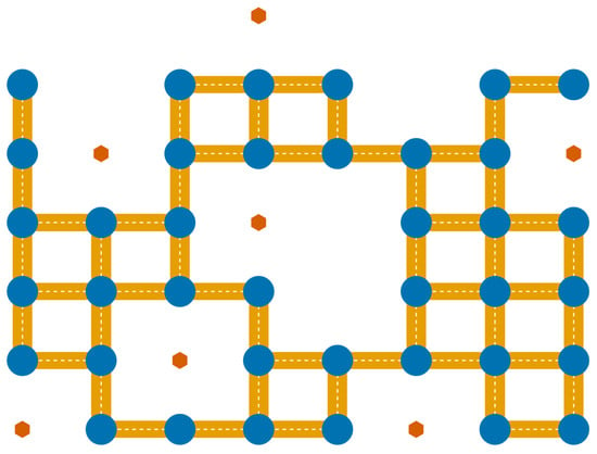
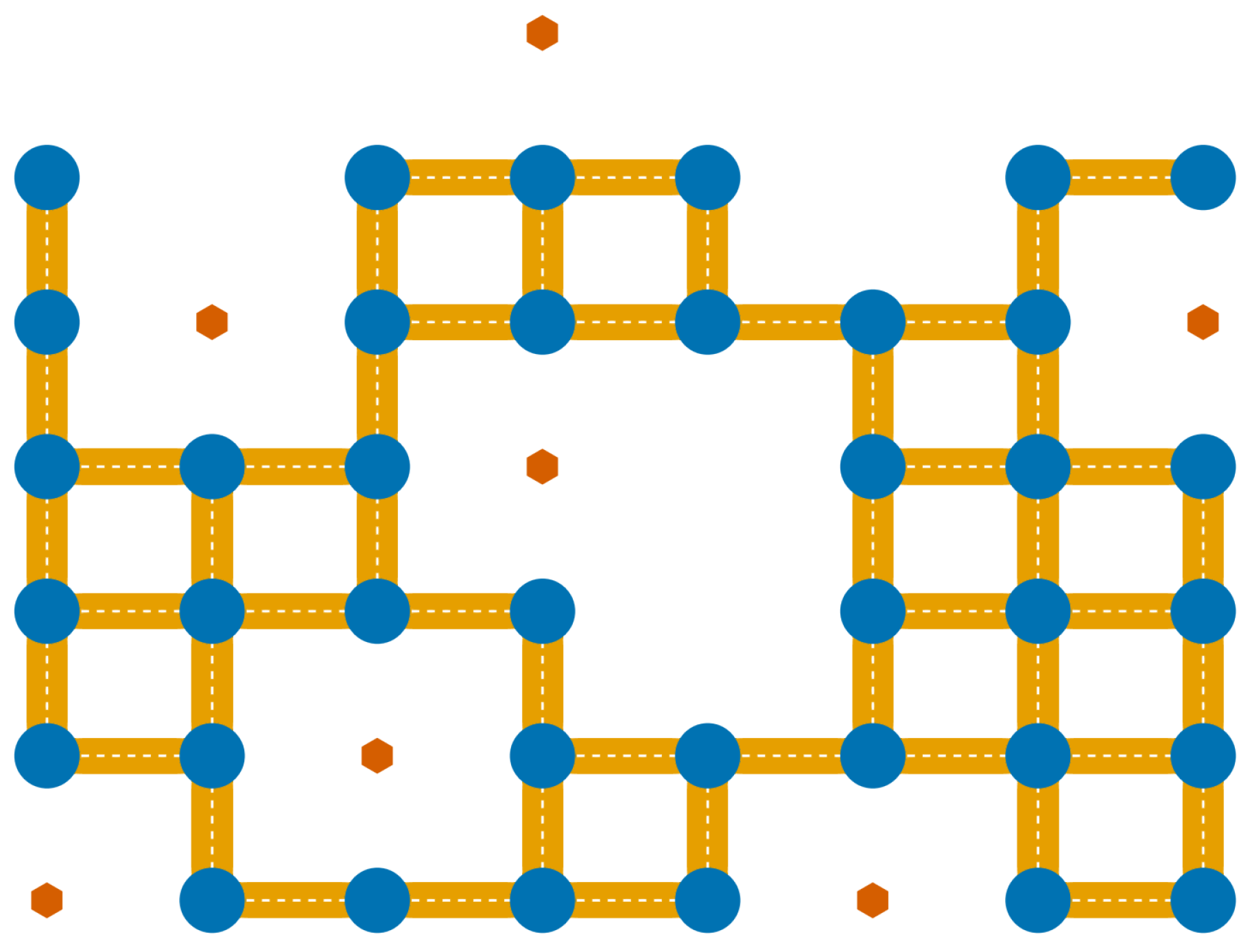
In , , we represent the road network as a directed graph , where is the set of nodes (intersections) and is the set of directed edges (roads) (Figure 1). Let be the complete probability space, where is the sample space, i.e., the set of all possible trajectories of a vehicle, is the -algebra on representing a set of measurable subsets of events, and is the probability measure on .
Figure 1.
An example of a road network. Blue color indicates the intersections, orange color indicates the roads, and red color indicates the stations monitoring the concentration of the pollutant.
Let the route of the mth vehicle be described by the function , where is time, , and M is the number of vehicles. Thus, the sample defines a set of trajectories , where .
In , we consider a fractional-order generalization of the convection–diffusion-reaction equation, which describes the dispersion of a pollutant in the atmosphere:
where is the pollutant concentration, , is the wind velocity field, is the vector of numerical parameters to be defined below, , and is the temporal Caputo fractional derivative:
and and are defined as follows:
where , , , is the atmospheric diffusion coefficient, and and are Riemann–Liouville fractional derivatives:
Including fractional derivatives with respect to the spatial variable in Equation (1) ensures that buildings and structures are taken into account, and including a fractional derivative with respect to the temporal variable ensures that the hereditary properties of the process are taken into account.
We note that the orders of fractional derivatives used in our study are representative of anomalous diffusion regimes observed in urban and turbulent atmospheric environments. Values of are commonly associated with subdiffusive memory effects, particularly in low-turbulence zones, where pollutants linger longer than predicted by classical models [36]. However, extremely low values of , particularly , correspond to excessively strong memory effects and subdiffusive behavior that are not representative of real atmospheric dispersion, even under stable or low-turbulence conditions. Such values tend to overly suppress temporal propagation and would lead to unrealistically slow dissipation of pollutants. Riesz spatial operators with have been shown to better capture heavy-tailed spatial dispersion patterns in field-scale experiments [58]. The use of in the first-order Riesz derivative reflects spatial nonlocality in advective transport, where influence is not limited to nearest neighbors, which is a feature often seen in urban atmospheric dynamics.
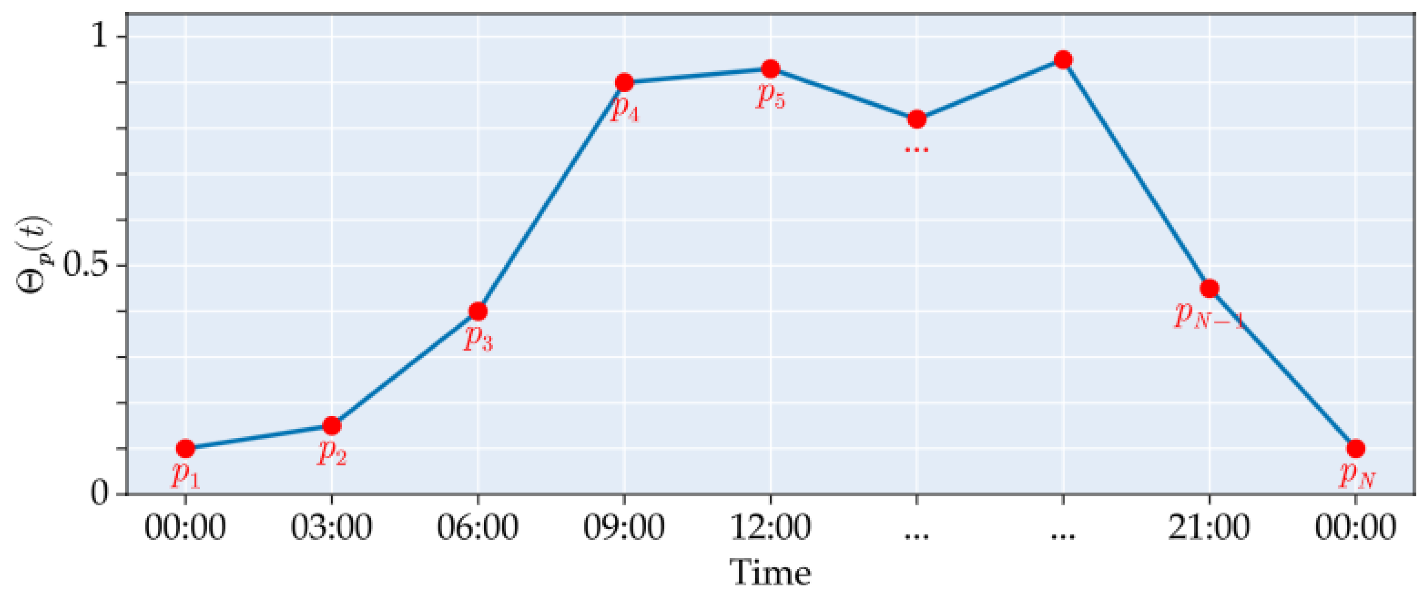
Now let us define the right-hand side of Equation (1). Each vehicle emits pollutants into the atmosphere as it moves, but their intensity may not be constant throughout the day. To take into account the time-varying activity of pollutant emissions, we introduce a scalar dimensionless modulation function , constructed as a piecewise linear function interpolating a sequence of points , where are discrete moments of time, and is the empirical representation of the temporal change in emission activity. Let and define the right-hand side of Equation (1) as follows:
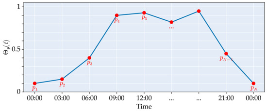
where is the pollution density of the mth vehicle. The physical meaning of the function is the normalized traffic intensity of vehicles over time (Figure 2). It scales emissions figures for all vehicles equally to reflect typical daily changes in traffic flow, such as morning and evening rush hours, lower traffic volumes at night, or possible temporary increases due to events.
Figure 2.
Schematic representation of the function .
The wind velocity field is determined from the Navier–Stokes equations for an incompressible fluid:
where is air pressure, and is the Reynolds number.
The choice of the boundary conditions is due to our use of a horizontal, depth-averaged two-dimensional urban model embedded in a large-scale atmospheric reservoir. We assume that the outer-boundary velocity equals the externally provided mesoscale wind , while the concentration is fixed to the observed background at the outer boundary.
Thus, the forward problem is formulated as follows:
Problem 1
Due to the stochastic nature of the problem, the statistical moments of the solution, such as expected concentration , concentration variance , or the probability of exceeding a certain threshold concentration , are of interest. This reduces to the need to repeatedly solve Problem 1 for randomly generated samples .
2.1.2. Statement of the Inverse Problem
In practice, the parameter vector is typically unknown and must be inferred. In this work, is estimated by formulating and solving an inverse problem constrained by observed pollutant concentration data.
Let us assume that contains S stations monitoring the concentration of a pollutant located at points (Figure 1). Let denote the concentration value measured by the sth station located at the point at time t.
We introduce the functional for quantitatively assessing the discrepancy between the predicted solution and the reference measurement data:
where denotes the expected value. Then, the inverse problem is formulated as follows:
Problem 2
(Inverse problem). Determine the parameter vector that minimizes the functional given in Equation (9).
2.2. Solution Method
2.2.1. Method of Solving the Deterministic Forward Problem
Let us start by discretizing Equation (1) at fixed and .
Let for , and . In addition, we introduce a uniform partition of the time interval for . Time will be referred to as the nth time layer. Let us denote by the value of the grid function at the node at time for fixed and . In addition, the vector of internal nodes will be used below:
To discretize the temporal fractional derivative in Equation (1), we use the approximation formula [59]:
where
There are several approximation formulas for discretizing the Riemann–Liouville fractional derivative. Since using the same Riemann–Liouville fractional derivative discretization formulas leads to an unstable scheme [35], we use different approximation formulas for the convective and diffusion parts. To discretize the convective term , we use the standard Grünwald–Letnikov formula, which for node has the following form [28]:
where the coefficients are defined as
To discretize the diffusion term, we use the L2-approximation method, which for node has the following form [60]:
To implement the algorithm numerically, it is convenient to switch to a matrix form. Let denote the Toeplitz matrix with the first column and the first row . Let us define the matrices
As a result, we arrive at the following matrix equation for the approximate solution of Equation (1) at the nth time layer:
where is the desired solution vector, defined as
and the matrix and the vector are defined as
where the properties of the coefficients are used [30], is the unit matrix, ⊗ stands for the Kronecker product, ⊕ denotes the Kronecker sum defined as , and . In addition, we use the upstream partition to discretize the convective term . Therefore, diagonal matrices are introduced that are formed from the positive and negative parts of the velocity components :
Let us now dwell on the implementation of the calculation of the right-hand-side vector . For each of the M simulated vehicles, we randomly assign a source–destination pair , , and compute the shortest path using Dijkstra’s algorithm.
To model the continuous movement of a vehicle along a discrete route , we apply linear interpolation between its successive nodes. Assuming that is the total duration of the vehicle’s trip, we divide it into intervals , where the time of the vehicle’s appearance on the road network is a random variable, and the subsequent time is determined as
where proportional to the length of the corresponding segment. Then, the trajectory is linearly defined piecewise as
The pollutant emitted by a vehicle is assumed to be distributed among nearby grid nodes by a discrete approximation of the Dirac delta function defined by a hat function centered at the vehicle position . Thus, the right-hand side function f is approximated as
and , and is a normalization parameter.
To solve Equations (3) and (4) we use the well-known approximation approach on a staggered grid according to the following algorithm, which includes three computational steps [61]:
where and are difference analogues of convective and turbulent exchange operators, is the discrete analogue of the del operator. The first computational step, expressed by Equation (15), takes into account only convective and turbulent exchange and calculates the intermediate velocity field . The second step (16) calculates the pressure field from the intermediate velocity field. In the third step (17), the velocity field is corrected taking into account the pressure gradient.
2.2.2. Method for Solving the Stochastic Forward Problem
Now let us fix the parameter vector . To solve the stochastic problem, we simulate independent realizations of and solve Problem 1 for each .
Note that the matrix in (13) is the same for all samples within a single time layer, which provides two key advantages. Firstly, this allows for solving the stochastic problem once for all samples at once, rather than solving it separately for each sample [62]. This comes down to solving a large number of systems of linear equations with the same coefficient matrix and different right-hand sides. Secondly, it makes it possible to use efficient factorization methods [44]. For this reason, an incomplete LU factorization preconditioner [63] is used to speed up the calculations.
2.2.3. Method for Solving the Inverse Problem
The parameter vector is identified through an iterative procedure based on the repeated solution of the forward problem and successive updates of the parameter values via an optimization algorithm. At each iteration j, the current estimate is used to solve Equation (1) subject to the boundary and initial conditions given in Equations (6) and (8) and with the corresponding right-hand side . The numerical solution obtained for this parameter set is then evaluated at the monitoring-station locations, and its deviation from the observed data is quantified by the discrepancy functional (9). This discrepancy provides a scalar objective value that guides the parameter update step. This process is repeated iteratively, forming a sequence , until a predefined convergence criterion is satisfied. Upon convergence, the final parameter vector is taken as the best-fit estimate with respect to the observed data and the given forward model.
In our previous paper [64], the applicability of a number of optimization algorithms, such as the conjugate gradient method [63], NEWUOA [65], BOBYQA [66], L-BFGS [67], and the Nelder–Mead method [68], was studied in detail. Based on numerous numerical tests, we came to the conclusion that the L-BFGS algorithm is more robust and allows identifying parameters in a wide class of functions and achieving greater accuracy. Moreover, its limited-memory structure makes it well-suited for high-dimensional problems, allowing for efficient handling of large parameter vectors without the need to store or invert full Hessian matrices. These advantages make L-BFGS particularly effective for the inverse problem considered in this study, where the parameter space is moderately large and the objective functional may be nonconvex.
2.2.4. Computational Algorithm
Thus, the proposed approach to solving the inverse Problem 2 consists of three stages, shown in Algorithm 1.
The algorithm takes the parameter L defining the domain, the final time T, the atmospheric diffusion coefficient , the Reynolds number , the initial and boundary conditions (5)–(8), the orders of fractional derivatives , the number of vehicles M, the number of parameters N, the number of realizations of the stochastic problem , the accuracy parameter and the maximum number of iterations as input parameters. We also assume that each component of the vector is bounded by positive numbers and .
Next, the algorithm consists of three main stages. At the first stage, the Navier–Stokes equations are solved to determine the velocity field at all time layers. The second preparatory stage involves generating the stochastic input data necessary for simulating multiple realizations. Specifically, random traffic routes are constructed for each realization , representing the spatial and temporal distribution of moving vehicles throughout the domain. Each vehicle is assigned a pollution density . Additionally, for each realization , an initial guess for the unknown parameter vector is randomly generated within the admissible parameter space. At the third stage, the iterative procedure described in Section 2.2.3 is carried out.
| Algorithm 1 Algorithm for solving the inverse problem |
|
3. Results
To analyze the model and computational algorithm for solving the inverse problem, a series of numerical tests has been carried out. All calculations were performed on a workstation with a 16-core AMD Ryzen 9 7950X3D processor with a clock frequency of 4.2 GHz, 128 GB of RAM, and a Gigabyte RTX 4090 graphics card with 24 GB of VRAM.
3.1. Analysis of the Forward Problem
3.1.1. Comparison of the Classical Convection–Diffusion Model with the Fractional Differential Model
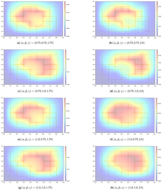
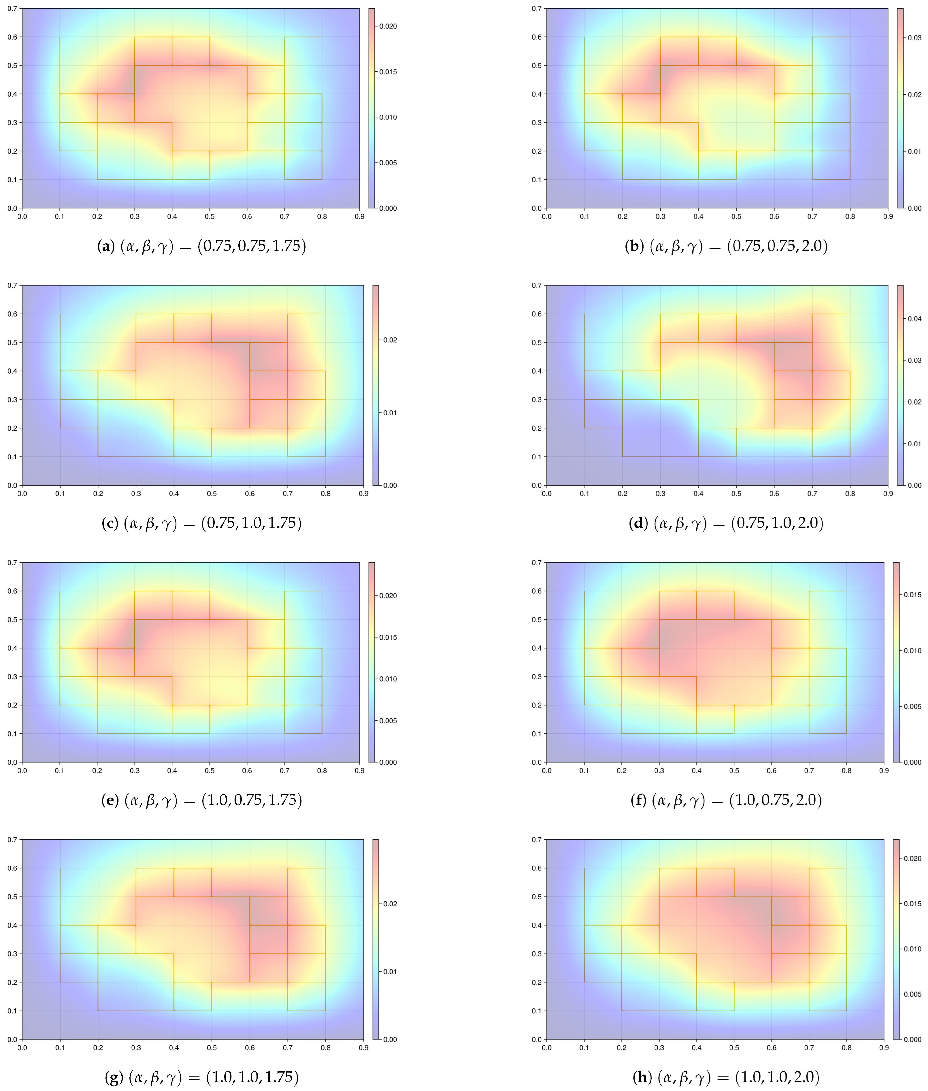
In the first computational experiment, an analysis of the forward problem was carried out. The aim of this computational experiment was to analyze the influence of fractional derivatives on the process of pollutant propagation. We considered a model problem in a unit square on a road network, which is represented by a graph shown in Figure 1. The following model parameters were adopted in this computational experiment: , . To focus on the influence of fractional derivatives, we chose a parameter vector in the form , which corresponds to the daily intensity profile of the pollutant sources, divided into eight three-hour intervals.
The classical case , shown in Figure 3h, serves as a reference, giving a smooth, centrally sharp concentration plume that spreads symmetrically with moderate gradients towards the boundaries. Deviations from this integer-order scenario clearly arise as the orders of fractional derivatives decrease.
Figure 3.
Effect of fractional derivatives on concentration at final time .
In cases where the temporal and spatial fractional orders are lower, the solution behavior reflects enhanced memory and reduced smoothing, which manifest as slower dissipation and more persistent pollutant presence at observation points. This aligns with known characteristics of anomalous transport processes: pollutants remain elevated longer and spread less uniformly, capturing realistic urban atmospheric effects, such as trapping in street canyons or delayed dispersion due to thermal inversions. Figure 3a–g clearly illustrate how variations in fractional orders shift not only the magnitude but also the temporal progression of concentration emphasizing that small deviations from integer-order behavior can lead to qualitatively different pollutant dynamics.
For example, when decreases to 0.75, the concentration dynamics slow down significantly, reflecting memory effects in time dynamics. Compared to the classical case, the jets for lower remain less developed at the same finite time, with lower-peak concentrations and smoother gradients. For example, comparing with shows that the former retains a broader, more diffuse appearance, indicating a slower accumulation of pollutants.
It can also be noted that decreasing from 1.0 to 0.75 reduces the intensity of convective transport. While the classic plume exhibits a pronounced directional tilt due to convection, a lower value yields a more symmetrical distribution. For example, the shape of the plume at appears more round and centered compared to the elongated structure in the classical case , which emphasizes the weakening of the directional drift.
Further, reducing from 2.0 to 1.75 shifts the system towards subdiffusion. This change limits spatial distribution and increases peak concentrations. For example, in the case of , the plume is more compact and maintains higher values in the center compared to the smoother, wider plume in the classical case. Thus, a lower concentrates the mass closer to the source, reflecting difficult scattering.
The cumulative effect of multiple order declines is particularly significant. In cases such as , highly localized plumes are observed with a noticeably smaller spatial spread and slower development compared to . In contrast, partial reductions, such as or , exhibit intermediate behavior: slower time evolution, reduced convection, or sharper peaks, depending on which order is decreasing.
3.1.2. Observation of Changes in Concentration at Stations: Transition from the Classical Model to the Fractional-Order Model
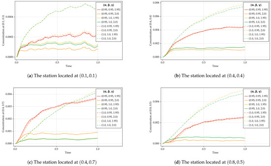
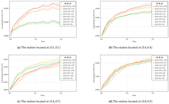
To evaluate the influence of integer-order and near-integer order derivatives on pollutant dispersion, we solved the forward problem for seven combinations of parameters , where , and . The change in concentration was monitored at four spatial points, , , , and , where stations were installed. The reason for choosing these points for analysis is that the first and fourth points are boundary points, the second is internal, and the third is external.
As can be seen from Figure 4, in all cases, the order of the fractional time derivative had the greatest impact on concentration levels. Even a moderate decrease in from 1 to 0.95 resulted in a significant increase in pollutant concentrations, indicating that the transition from fractional to integer time dynamics significantly accelerates pollutant accumulation. Integer-order time derivatives resulted in a two-fold increase in peak concentrations compared to fractional-order cases, especially in the inner region.
Figure 4.
The influence of orders of fractional derivatives on the process of dispersion of a pollutant in the atmosphere: comparison of classical and fractional-order models.
Spatial fractional orders and also influenced concentration profiles, but to a lesser extent. Higher and values tend to reduce peak concentrations, reflecting increased diffusive transport that more efficiently disperses pollutants. The differences between and were small but consistent, with slightly lower concentrations for the integer case . Changes in showed similar trends, with resulting in slightly less pollutant retention than .
At the boundary point , concentrations generally remained low, although integer-order time derivatives still yielded substantially higher values than fractional cases, demonstrating a persistent influence even near the domain edges. In the interior regions, such as at and , the combined effects of , , and become more pronounced, with higher values and lower spatial orders leading to greater pollutant accumulation. Further from the source, as at , the influence of spatial fractional orders remained evident but was comparatively diminished, while continued to dominate the concentration levels.
Note that the fluctuations observed in the concentration curves at low fractional orders arise because the fractional derivatives impose a strong memory and non-local transport effect that reduces the natural damping present in classical diffusion. As a result, even small physical or numerical perturbations can persist and propagate, leading to visible temporary fluctuations in predicted concentrations.
3.1.3. Analysis of the Influence of Lower Orders of Fractional Derivative on the Pollutant Dispersion Process
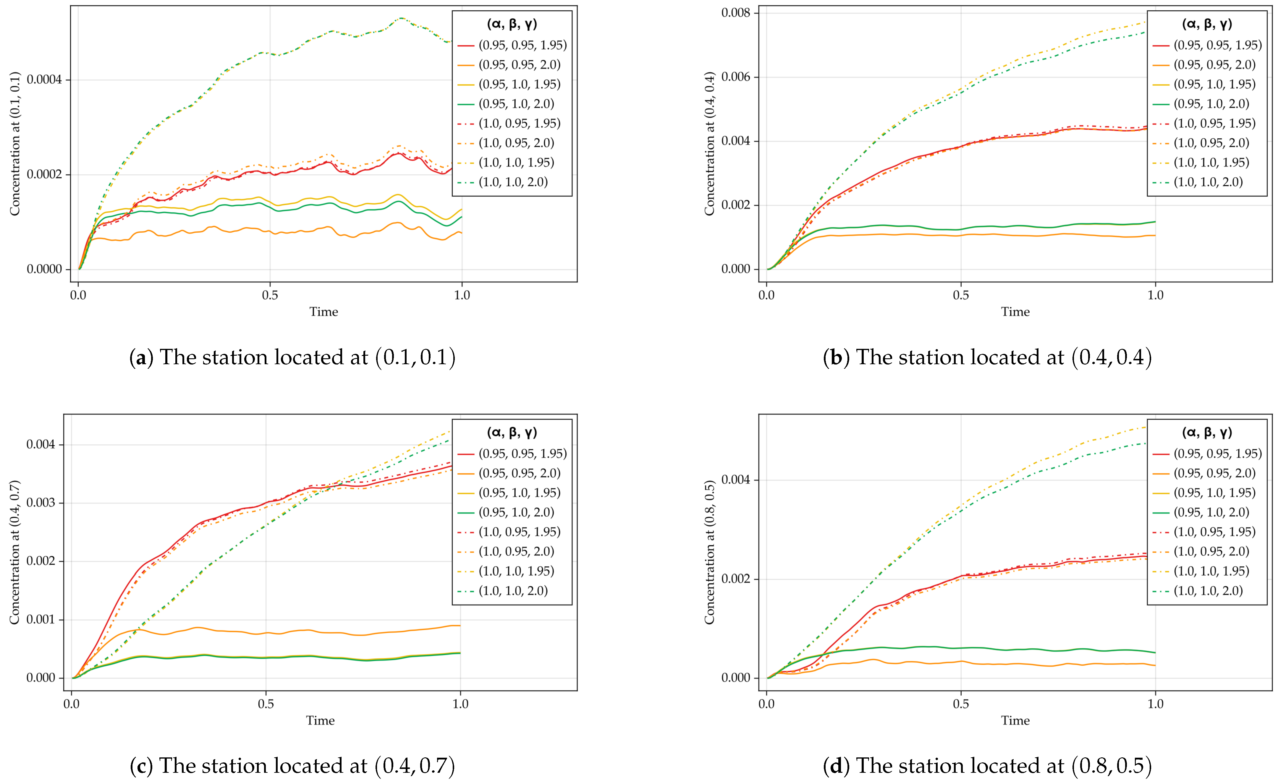
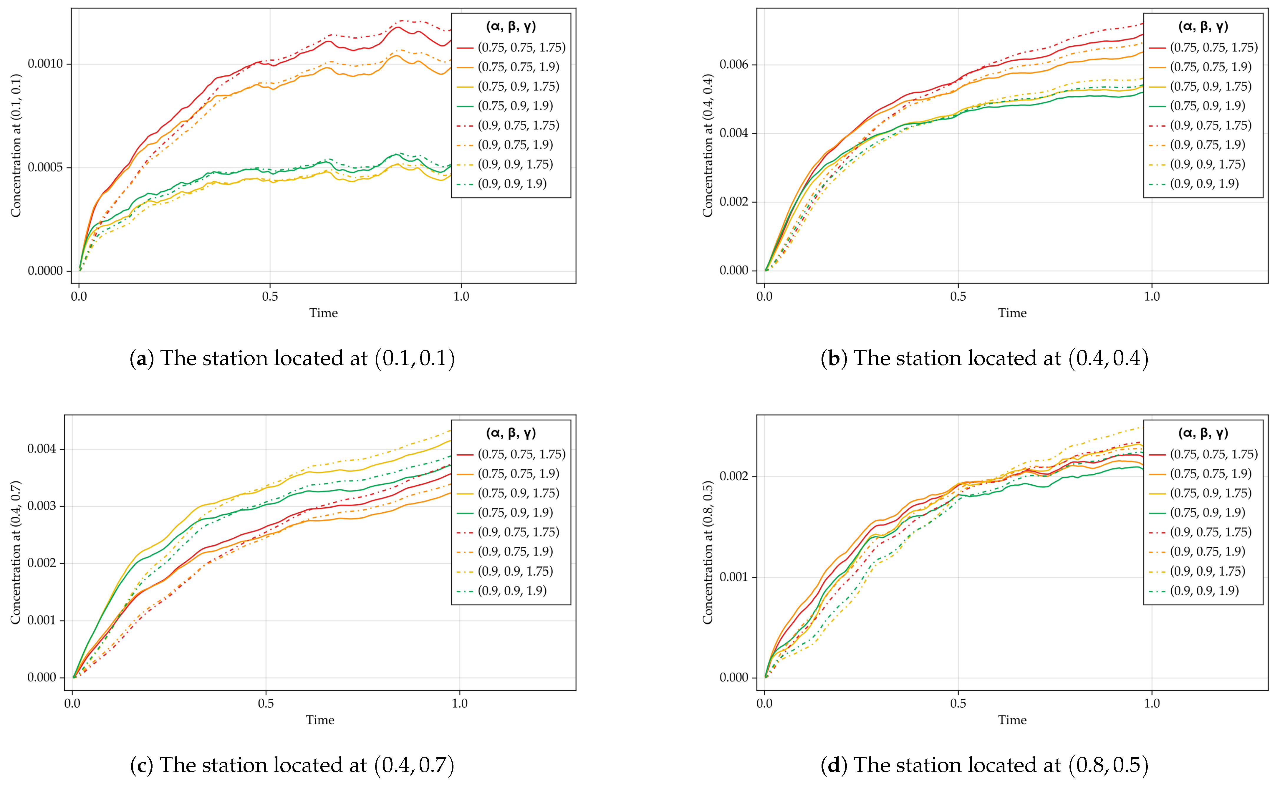
To investigate how lower fractional orders affect pollutant dispersion, we analyzed concentrations at four spatial points for eight combinations of with reduced orders compared to the classical case and the previously studied slightly fractional case .
It can be seen from Figure 5 that further reduction of the orders of the time derivative to 0.75 and the spatial derivatives and to 0.75 and 1.75, respectively, significantly slows down the dispersion process and leads to significantly higher concentrations of pollutants that persist over time.
Figure 5.
The influence of orders of fractional derivatives on the process of dispersion of a pollutant in the atmosphere.
At all four observation points, a lower causes a more pronounced memory effect, resulting in concentrations initially rising faster and remaining elevated longer, which is particularly noticeable in the curves for . Reducing from 1.95 to 1.75 reduces diffusion, further enhancing the retention of pollutant mass around the source. This is particularly noticeable at points close to the origin, such as , where peak concentrations exceed the values observed for and , confirming weaker scattering. Meanwhile, decreasing reduces the effect of convection, slightly delaying the outward transport of the pollutant, resulting in more localized peaks and slower propagation, especially at the periphery, for example, .
Overall, compared to the near-classical case , further decreasing orders leads to stronger localization of the pollutant plume and higher residual concentrations at all points, emphasizing that the choice of low fractional orders significantly changes both the dynamics and the possible spread of pollutants in the atmosphere.
Note that low fractional orders (especially ) lead to unrealistic concentrations of pollutants and excessive spatial distribution, which contradicts the physical processes of turbulent diffusion. Therefore, such low orders are not suitable for modeling the dispersion of atmospheric impurities within the framework of this model.
3.1.4. Influence of Parameters on the Spread of a Pollutant
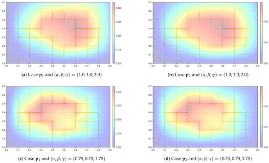
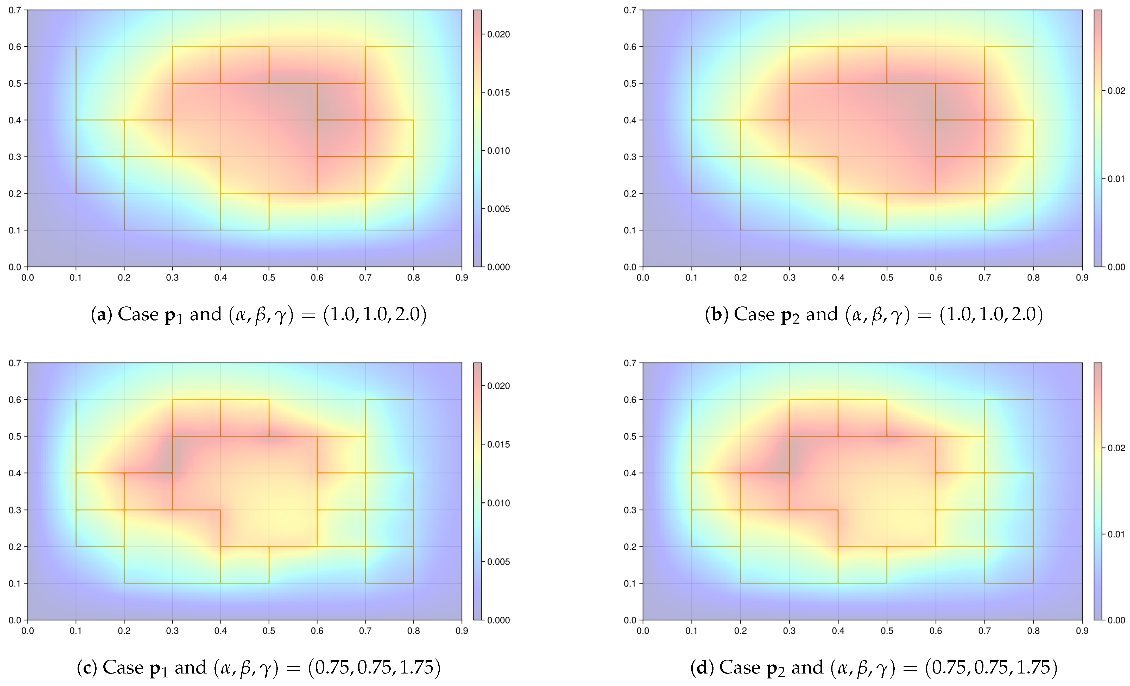
To analyze the influence of the parameters on the spread of the pollutant, a series of numerical experiments were carried out. We limited ourselves to considering two parameter vectors, and , that define the daily intensity profile of pollutant sources, divided into eight three-hour intervals.
It follows from Figure 6a that in the classical convection–diffusion equation the uniform vector leads to a spatially symmetric concentration distribution with a maximum at the center of the domain and relatively uniform gradients. On the contrary, the use of a non-uniform vector (Figure 6b) induces pronounced spatial inhomogeneities: the maximum concentration shifts to the region corresponding to the total contribution of time intervals with increased emission intensity values, forming local peaks and sharp gradients.
Figure 6.
Analysis of the influence of parameters on the spread of a pollutant under classical and fractional differential models.
For a fractional differential equation (Figure 6c,d), a characteristic smoothing of the spatial distribution of concentration is observed due to the memory effect and subdiffusion/superdiffusion behavior: maximum concentration values decrease, local extrema are leveled out, and the distribution takes on a more diffuse shape. Thus, fractional derivatives reduce the sensitivity of the solution to daily fluctuations in emission intensity, whereas in the classical formulation, fluctuations in the parameters are directly reflected in the spatial structure of the concentration field.
3.2. Stability and Convergence of the Numerical Method
The following numerical tests were aimed at determining the convergence order of the numerical method (13). Since the exact solution is unknown, the empirical convergence order was estimated using a self-consistency method based on successive mesh refinement. Numerical solutions were calculated on five grids with steps , , , , at a fixed spatial step . Next, the empirical convergence order was calculated using the following formula:
To determine the convergence order with respect to the spatial variable, a similar technique was used with a fixed time step .
We limited ourselves to considering one case of orders of fractional derivatives, , , . Due to the use of an approximation Formula (10) of order , the expected convergence order in the temporal variable was 1.2, and due to the use of an approximation Formula (11) of order , the expected convergence order in the spatial variable was 1.
The results of the computational experiments presented in Table 1 are in good agreement with theoretical assumptions.
Table 1.
Convergence analysis of the numerical scheme.
Since the scheme is fully implicit, it was expected to be unconditionally stable, and no CFL-type coupling between the time step and the grid size h was required. In practice, our calculations were stable over a wide range of and h. We did not observe any unphysical growth or oscillations in all the numerical tests we performed.
3.3. Evaluation of the Efficiency of the Algorithm for Solving the Inverse Problem
To evaluate the efficiency and reliability of the proposed method for solving the inverse problem, we conducted a series of numerical experiments. We generated 1000 random samples of the true parameter vector governing the right-hand side of the convection–diffusion equation modeling the dispersion of pollutants in the atmosphere. For each sample, we solved the forward problem and then applied our iterative inverse method, initialized based on a common initial guess, to infer the unknown coefficients. In this experiment, the vector consisted of six unknown coefficients, and the vector was chosen as the initial guess.
Our analysis focused on four key performance indicators.
3.3.1. Convergence Behavior
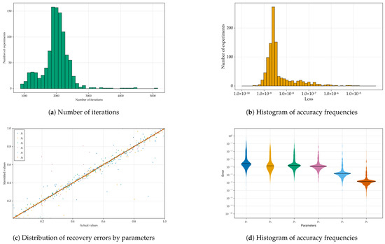
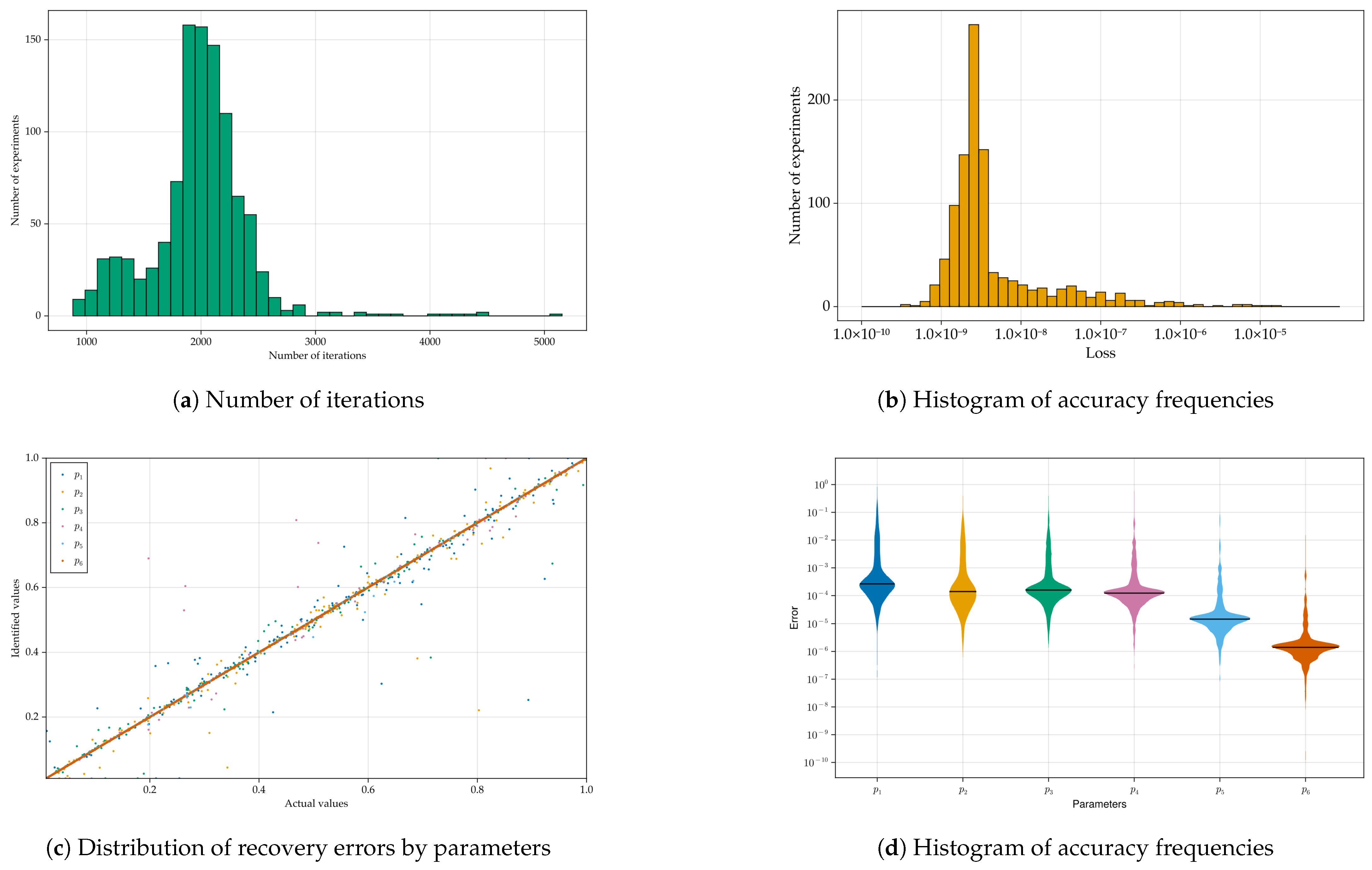
We recorded the number of iterations required for the L-BFGS algorithm to reach convergence for each of the 1000 inverse problems. The histogram shown in Figure 7a displays the frequency distribution of the number of iterations. In most cases, convergence was achieved within 1500–2500 iterations, indicating stable and efficient convergence. Only in a small proportion of cases did the number of iterations exceed 3000, suggesting sometimes slow convergence, possibly due to unfavorable initial approximations or poor conditioning in certain parameter regions.
Figure 7.
Analysis of efficiency of the algorithm for solving the inverse problem.
3.3.2. Accuracy of the Derived Coefficients
To assess the accuracy of the inferred parameters, we calculated the absolute and relative errors between the inferred coefficients and the corresponding true values for each sample. The histogram of relative errors (Figure 7b) shows that for most experiments the absolute error remained below , demonstrating the good ability of the algorithm to recover parameters. A small number of outliers with higher errors were found, which may indicate local minima or insensitivity of the forward model to certain parameter changes.
3.3.3. Scatter Plot of Actual and Expected Coefficients
Figure 7c shows a scatter plot comparing the true parameter values with the corresponding predicted values for all 1000 samples. Ideally, the points should lie along the identity line , indicating perfect parameter recovery. The graph shows a strong linear correlation, confirming that the inverse method reliably recovers the true coefficients in most cases. Deviations from the diagonal highlight the magnitude of the inference errors and reveal areas where the method could benefit from further regularization or more informative initial guesses.
3.3.4. Violin Plot of Accuracy Depending on the Parameter
To examine the variability of inference accuracy under different unknown parameters, we constructed violin plots of the relative errors in estimating each of the six unknown coefficients. The violin plots shown in Figure 7d, illustrate both the density distribution and the error spread for each parameter.
The graphs show that while most parameters are derived with consistently low relative errors, some parameters exhibit wider distributions, indicating higher uncertainty or variability in the estimation process. For example, the first parameters exhibit a somewhat wider distribution, suggesting that they may be less identifiable from the available data or more sensitive to initial guesses and measurement noise.
3.4. Sensitivity to Parameters Initialization
To investigate the sensitivity of the solution of the inverse problem to the choice of initial approximations, we conducted an additional series of experiments. In this case, we fixed a set of true parameters , shown in Table 2 and defining the right-hand side of the convection–diffusion equation, and solved the inverse problem 100 times, each time starting from a random initial guess. Our analysis included three key assessments.
Table 2.
The set of parameters used in the computational experiment of Section 3.4.
3.4.1. Histogram of the Number of Iterations
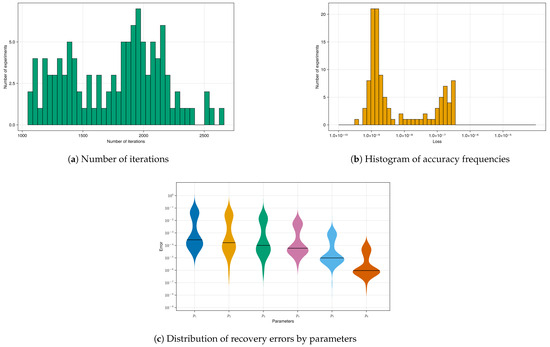
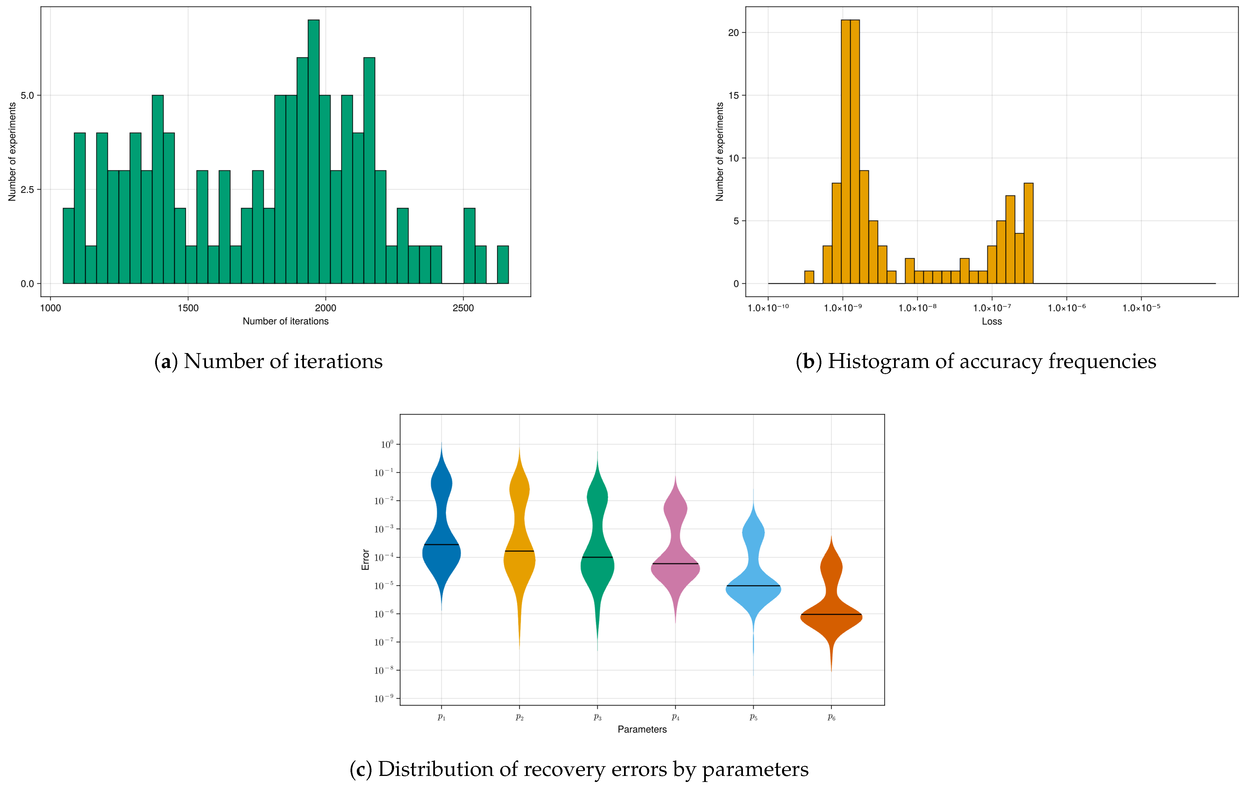
Figure 8a shows a histogram showing the number of iterations required to converge over 100 runs. The distribution shows that, while most runs converge in the same number of iterations, in some cases, significantly more iterations are required to achieve convergence. This suggests that while the algorithm is generally stable, some initial guesses may lead to longer optimization paths, possibly due to proximity to local minima or flat regions in the loss landscape.
Figure 8.
Analysis of sensitivity to parameter initialization.
3.4.2. Histogram of Inference Accuracy
Figure 8b shows a histogram of the relative errors between the inferred parameters and the fixed true parameters. Most runs achieve low levels of inference errors, indicating the ability of the method to recover the true parameters despite changing initial conditions.
3.4.3. Violin Plot of Parameter-Specific Accuracy
To investigate how sensitivity varies with different parameters, we plotted relative errors for each of the six unknown coefficients (Figure 8c). The violin plots show that while some parameters are consistently well recovered regardless of the starting point, others exhibit a wider distribution, indicating greater sensitivity to the initial guess.
4. Discussion
Let us make a few comments regarding the obtained results in the context of previous studies. First of all, our results obtained in Section 3.1 have noticeable similarities with the results of fractional modeling of transport through porous media [30,69,70], where fractional derivatives have been successfully used to account for anomalous diffusion, memory effects, and non-local transport. Just as porous structures result in long residence times and heavy tails in concentration profiles [30], urban atmospheres, characterized by complex geometries, flow barriers, and heterogeneous sources, exhibit slow dispersion and non-Gaussian spread of pollutants. In both cases, the Caputo time derivatives model memory-induced delays in response to sources, while the Riesz spatial derivatives reflect non-local spreading beyond what classical Fickian diffusion can represent.
However, a key difference is that in porous media flow paths are typically static and tortuous, whereas in urban atmospheres pollutant sources are mobile and emission patterns change over time. Such dynamic behavior, in particular the use of time-varying line sources associated with moving vehicles, has been largely absent from existing fractional transport models. Our work extends the applicability of fractional PDEs by including stochastic and time-modulated emissions, providing a more realistic basis for predicting urban air quality.
Our numerical results are consistent with previous studies, demonstrating that fractional derivatives offer a more flexible and accurate framework for modeling anomalous transport phenomena. Similar to the results of porous media flow studies (for example, [71]), we observe that the reduction in time order leads to memory effects that delay pollutant dispersion and result in maintenance of concentration levels, consistent with the results of [58,72,73]. Similarly, decreasing the spatial orders of and leads to a non-Gaussian spread and heavier concentration tails, consistent with observations in fractional atmospheric diffusion models [74]. However, unlike most previous studies that assume fixed or point sources of pollutants, our work includes dynamic line sources associated with vehicle traffic, resulting in more realistic and spatially heterogeneous concentration models.
While some earlier works have used fractional models exclusively in forward modeling, our study considers the inverse problem for reconstructing time-dependent emission profiles, an aspect that has been largely unexplored in the context of fractional PDEs for urban air pollution. These differences highlight the novelty of our approach in both source modeling and the integration of fractional dynamics with parameter inference.
Traditional inverse modeling of air pollutant emissions has largely relied on adjoint-based variational methods [75,76], ensemble Kalman filters [77], and Bayesian inference frameworks [78]. These methods are well-suited for large-scale or regional applications where Gaussian assumptions and integer-order transport models are appropriate. However, they require complex adjoint solvers or large ensemble sizes and often assume Markovian dynamics. In contrast, our approach integrates optimization-based parameter estimation with a fractional-order convection–diffusion-reaction model, enabling us to capture nonlocal transport effects and temporal memory without relying on detailed adjoints or covariance tuning.
Compared with previous studies, our approach to solving the inverse problem has a number of clear advantages. Although many studies focus on source identification within classical diffusion models (for example, [79]), they typically assume static or point sources and often use simplified time profiles. In contrast, our method successfully reconstructs the time-varying radiation intensity associated with moving line sources under the additional complexity of fractional-order dynamics. This situation introduces non-locality both in space and time, which makes the inverse problem more difficult. Despite this, our results show that the parameters governing the time-modulated emissions can still be recovered with good accuracy from sparse sensor data, highlighting the robustness of the proposed inference framework. To our knowledge, inverse modeling for such systems, combining fractional convection–diffusion equations with stochastic vehicle emissions, has not been considered in previous studies.
5. Conclusions
In conclusion, our study shows that a fractional-order convection–diffusion-reaction formulation with Caputo temporal memory and Riesz spatial nonlocality provides a physically interpretable representation of anomalous dispersion, heavy tails, and persistence in urban flows, features under-represented by classical integer-order convection–diffusion-reaction models. Our numerical results indicate that the fractional model captures long-range transport and persistent pollutant effects more effectively than the classical model, particularly near sources and at downwind receptors. Although our method is more computationally expensive compared to the integer-order model due to the need to discretize temporal Caputo fractional derivative, which makes identifiability more sensitive to sensor density and placement, it reduces structural model error and improves agreement with observations, yielding more reliable emission-activity estimates. By estimating time-varying emission activity via regularized optimization, we isolate the role of the forward physics and avoid the need to develop an adjoint for nonlocal, history-dependent operators. Overall, our main contributions are a systematic analysis of how fractional orders shape plume propagation and residual structure, and evidence that a compact time–activity parameterization suffices to reconcile observations at city scale.
Our research also contributes to several United Nations Sustainable Development Goals, particularly Goal 3 (Good Health and Well-Being), Goal 11 (Sustainable Cities and Communities), and Goal 13 (Climate Action), by advancing modeling techniques that can support urban air quality management and inform pollution mitigation strategies.
Although this study focuses on synthetic numerical experiments, future work will include validation of the proposed model using real-world data, such as urban air quality measurements and traffic flow records. This will enable a more rigorous assessment of predictive accuracy and parameter identifiability under realistic conditions. The authors also plan to combine the results of this work with the results of a previous paper [64], in which machine learning algorithms were used to predict concentrations at monitoring stations. It is expected that this approach will allow for achieving even more accurate results to solve the inverse problem under consideration. Further, the authors intend to explore the use of physics-informed neural networks [80] as an alternative framework for inferring model parameters, with the goal of improving scalability, accommodating sparse or noisy data, and enabling more flexible representations of time-varying emission activity.
Author Contributions
Conceptualization, M.M. and N.A.; methodology, M.M.; software, M.M.; validation, N.A. and A.B.; formal analysis, G.M.; investigation, M.M.; resources, M.M.; data curation, M.M.; writing—original draft preparation, N.A.; writing—review and editing, N.A.; visualization, Y.Y.; supervision, M.M.; project administration, M.M.; funding acquisition, M.M. All authors have read and agreed to the published version of the manuscript.
Funding
This research has been funded by the Science Committee of the Ministry of Science and Higher Education of the Republic of Kazakhstan (Grant No. AP19679550).
Institutional Review Board Statement
Not applicable.
Informed Consent Statement
Not applicable.
Data Availability Statement
Data are contained within the article.
Conflicts of Interest
The authors declare no conflicts of interest.
Nomenclature
| the spatial domain [] | |
| the finite difference grid introduced in the spatial domain | |
| the Caputo fractional differentiation operator | |
| the Riemann-Liouville fractional differentiation operator | |
| the set of edges | |
| the -algebra | |
| the directed graph | |
| the unit matrix | |
| h | the discretization parameter of the spatial domain |
| L | the side length of the spatial domain [m] |
| M | the number of vehicles |
| the number of nodes in each direction of the finite difference grid | |
| the number of nodes in the uniform partition of the time interval | |
| the probability measure | |
| the vector of parameters | |
| the parameter indicating the empirical representation of the temporal change in emission activity [dimensionless] | |
| T | the final time [s] |
| a uniform partition of the time interval | |
| the Toeplitz matrix with the first column and the first row | |
| the wind velocity field [m/s] | |
| the set of nodes | |
| the position of the mth vehicle | |
| the node of the finite difference grid | |
| the vector of internal nodes of the finite difference grid | |
| the order of the temporal Caputo fractional derivative | |
| the order of the spatial Riesz fractional derivative | |
| the order of the spatial Riesz fractional derivative | |
| the atmospheric diffusion coefficient [] | |
| the wind pressure [Pa] | |
| the pollutant emission rate of the mth vehicle [kg/s] | |
| the contaminant concentration [] | |
| the grid function representing the contaminant concentration | |
| the discretization parameter of the time segment (time step) | |
| the modulation function [dimensionless] | |
| the finite difference grid introduced in the segment | |
| the sample space | |
| a sample | |
| ⊗ | the Kronecker product |
| ⊕ | the Kronecker sum |
References
- Seesaard, T.; Kamjornkittikoon, K.; Wongchoosuk, C. A comprehensive review on advancements in sensors for air pollution applications. Sci. Total Environ. 2024, 951, 175696. [Google Scholar] [CrossRef] [Scilit]
- Samsudin, M.S.; Azid, A.; Razik, M.A.; Zaudi, M.A.; Shaharudin, S.M. Source of apportionment of air quality parameters at federal port of Malaysia with emphasis on ship emission. IOP Conf. Ser. Earth Environ. Sci. 2021, 810, 012052. [Google Scholar] [CrossRef] [Scilit]
- Sokhi, R.; Baklanov, A.; Mahura, A. Integrated Systems of Meso-Meteorological and Chemical Transport Models; Springer: Berlin/Heidelberg, Germany, 2011. [Google Scholar] [CrossRef] [Scilit]
- Stockie, J.M. The mathematics of atmospheric dispersion modeling. SIAM Rev. 2011, 53, 349–372. [Google Scholar] [CrossRef] [Scilit]
- Seinfeld, J.H.; Pandis, S.N. Atmospheric Chemistry and Physics: From Air Pollution to Climate Change, 3rd ed.; John Wiley & Sons: Hoboken, NJ, USA, 2016. [Google Scholar]
- Gireesh Kumar, P.; Lekhana, P.; Tejaswi, M.; Chandrakala, S. Effects of vehicular emissions on the urban environment—A state of the art. Mater. Today Proc. 2021, 45, 6314–6320. [Google Scholar] [CrossRef] [Scilit]
- Hassan, N.A.; Hashim, J.H.; Wan Puteh, S.E.; Wan Mahiyuddin, W.R.; Mohd, M.S.F.; Shaharudin, S.M.; Mohammad Aidid, E.; Sapuan, I. Investigation of the impacts of climate change and rising temperature on food poisoning cases in Malaysia. PLoS ONE 2023, 18, e0283133. [Google Scholar] [CrossRef] [Scilit]
- Ferragut, L.; Asensio, M.I.; Cascón, J.M.; Prieto, D.; Ramírez, J. An efficient algorithm for solving a multi-layer convection–diffusion problem applied to air pollution problems. Adv. Eng. Softw. 2013, 65, 191–199. [Google Scholar] [CrossRef] [Scilit]
- Ruhiat, Y.; Guntara, Y. Regional detection polluted with diffusion and convection models in Banten province. J. Phys. Conf. Ser. 2020, 1428, 012051. [Google Scholar] [CrossRef] [Scilit]
- Habingabwa, M.E.N.; Ndahayo, F.; Berntsson, F. Air pollution tracking using PDEs. Rwanda J. 2012, 27. [Google Scholar] [CrossRef] [Scilit]
- Ioannidis, G.; Li, C.; Tremper, P.; Riedel, T.; Ntziachristos, L. Application of CFD modelling for pollutant dispersion at an urban traffic hotspot. Atmosphere 2024, 15, 113. [Google Scholar] [CrossRef] [Scilit]
- Kafle, J.; Adhikari, K.P.; Poudel, E.P. Air pollutant dispersion using advection-diffusion equation. Nepal J. Environ. Sci. 2024, 12, 1–6. [Google Scholar] [CrossRef] [Scilit]
- Temirbekov, N.; Malgazhdarov, Y.; Tokanova, S.; Amenova, F.; Baigereyev, D.; Turarov, A. Information technology for numerical simulation of convective flows of a viscous incompressible fluid in curvilinear multiply connected domains. J. Theor. Appl. Inf. Technol. 2019, 97, 3166–3177. [Google Scholar]
- Patankar, S.V. Numerical Heat Transfer and Fluid Flow; CRC Press: Boca Raton, FL, USA, 2018. [Google Scholar]
- Bottoni, M. Numerical Methods for the Solution of the Convection-Diffusion Equation and QUICK Algorithm; Springer International Publishing: Cham, Switzerland, 2021; pp. 155–215. [Google Scholar] [CrossRef] [Scilit]
- Lapina, O.N.; Nesterenko, A.G.; Nikitin, Y.G.; Pavlova, A.V. Modelling of the diffusion-convection process of a pollutant with a periodic source. Ecol. Bull. Res. Centers Black Sea Econ. Coop. 2022, 19, 26–35. [Google Scholar] [CrossRef] [Scilit]
- Issakhov, A.; Alimbek, A.; Abylkassymova, A. Numerical modeling of water pollution by products of chemical reactions from the activities of industrial facilities at variable and constant temperatures of the environment. J. Contam. Hydrol. 2023, 252, 104116. [Google Scholar] [CrossRef] [Scilit]
- Li, L.; Yin, Z. Numerical simulation of groundwater pollution problems based on convection diffusion equation. Am. J. Comput. Math. 2017, 7, 350–370. [Google Scholar] [CrossRef] [Scilit]
- Rashidinia, J.; Momeni, A.; Molavi-Arabshahi, M. Solution of convection-diffusion model in groundwater pollution. Sci. Rep. 2024, 14, 2075. [Google Scholar] [CrossRef] [Scilit] [PubMed]
- Li, Z.; Lu, W.; Huang, J. Monitoring, diffusion and source speculation model of urban soil pollution. Processes 2020, 8, 1339. [Google Scholar] [CrossRef] [Scilit]
- Konshin, O.V. Applicability of the convection-diffusion mechanism for modeling migration of 137cs and 90sr in the soil. Health Phys. 1992, 63, 291–300. [Google Scholar] [CrossRef] [Scilit]
- Thenmozhi, D.; Eswara Rao, M.; Renuka Devi, R.L.V.; Nagalakshmi, C.; Selvi, P.D. Dynamics of heat transfer in complex fluid systems: Comparative analysis of Jeffrey, Williamson and Maxwell fluids with chemical reactions and mixed convection. Int. J. Thermofluids 2024, 24, 100896. [Google Scholar] [CrossRef] [Scilit]
- Zhao, B. Fundamental heat and entropy transfer mechanisms of convection underlying the first and second laws for an unsteady multiport system and their applications in parallel flow heat exchangers. Int. J. Heat Fluid Flow 2024, 107, 109400. [Google Scholar] [CrossRef] [Scilit]
- Meng, X.; Huang, M.; Wang, B.; Ouyang, X.; Huang, Y.; Chen, D.; Cheng, Y.; Li, Y. A numerical method for two-dimensional transient nonlinear convection-diffusion equations. Ann. Nucl. Energy 2024, 205, 110604. [Google Scholar] [CrossRef] [Scilit]
- Kanatani, K. Effects of convection and diffusion of the vapour in evaporating liquid films. J. Fluid Mech. 2013, 732, 128–149. [Google Scholar] [CrossRef] [Scilit]
- Kirsch, V.A. Numerical simulation of convective diffusion of point particles in a laminar flow past a row of profiled hollow fibers. Fibers 2022, 10, 77. [Google Scholar] [CrossRef] [Scilit]
- Pope, C.A.; Dockery, D.W. Health effects of fine particulate air pollution: Lines that connect. J. Air Waste Manag. Assoc. 2006, 56, 709–742. [Google Scholar] [CrossRef] [Scilit]
- Podlubny, I. Fractional Differential Equations; Academic Press: San Diego, CA, USA, 1999. [Google Scholar]
- Tarasov, V. Fractional Dynamics: Application of Fractional Calculus to Dynamics of Particles, Fields and Media; Springer: London, UK; New York, NY, USA, 2011. [Google Scholar]
- Baigereyev, D.; Alimbekova, N.; Berdyshev, A.; Madiyarov, M. Convergence analysis of a numerical method for a fractional model of fluid flow in fractured porous media. Mathematics 2021, 9, 2179. [Google Scholar] [CrossRef] [Scilit]
- Alimbekova, N.; Berdyshev, A.; Baigereyev, D. Parallel implementation of the algorithm for solving a partial differential equation with a fractional derivative in the sense of Riemann-Liouville. In Proceedings of the 2021 IEEE International Conference on Smart Information Systems and Technologies (SIST), Nur-Sultan, Kazakhstan, 28–30 April 2021; pp. 1–6. [Google Scholar] [CrossRef] [Scilit]
- Moreira, D.; Xavier, P.; Palmeira, A.; Nascimento, E. New approach to solving the atmospheric pollutant dispersion equation using fractional derivatives. Int. J. Heat Mass Transf. 2019, 144, 118667. [Google Scholar] [CrossRef] [Scilit]
- Troparevsky, M.I.; Muszkats, J.P.; Seminara, S.A.; Zitto, M.E.; Piotrkowski, R. Modeling particulate pollutants dispersed in the atmosphere using fractional turbulent diffusion. Phys. A Stat. Mech. Its Appl. 2022, 599, 127478. [Google Scholar] [CrossRef] [Scilit]
- Palmeira, A.; Xavier, P.; Moreira, D. Simulation of atmospheric pollutant dispersion considering a bi-flux process and fractional derivatives. Atmos. Pollut. Res. 2020, 11, 57–66. [Google Scholar] [CrossRef] [Scilit]
- Yang, Q.; Liu, F.; Turner, I. Numerical methods for fractional partial differential equations with Riesz space fractional derivatives. Appl. Math. Model. 2010, 34, 200–218. [Google Scholar] [CrossRef] [Scilit]
- Metzler, R.; Klafter, J. The random walk’s guide to anomalous diffusion: A fractional dynamics approach. Phys. Rep. 2000, 339, 1–77. [Google Scholar] [CrossRef] [Scilit]
- Metzler, R.; Klafter, J.; Sokolov, I.M. Anomalous transport in external fields: Continuous time random walks and fractional diffusion equations extended. Phys. Rev. E 1998, 58, 1621–1633. [Google Scholar] [CrossRef] [Scilit]
- Kallianpur, G.; Xiong, J. Stochastic models of environmental pollution. Adv. Appl. Probab. 1994, 26, 377–403. [Google Scholar] [CrossRef] [Scilit]
- Cheng, K.-C.; Acevedo-Bolton, V.; Jiang, R.-T.; Klepeis, N.E.; Ott, W.R.; Kitanidis, P.K.; Hildemann, L.M. Stochastic modeling of short-term exposure close to an air pollution source in a naturally ventilated room: An autocorrelated random walk method. J. Expo. Sci. Environ. Epidemiol. 2013, 24, 311–318. [Google Scholar] [CrossRef] [Scilit]
- Calvert, S.C. Stochastic Macroscopic Analysis and Modelling for Traffic Management. Ph.D. Thesis, Delft University of Technology, Delft, The Netherlands, 2016. [Google Scholar] [CrossRef] [Scilit]
- Xiu, D.; Karniadakis, G.E. The Wiener—Askey polynomial chaos for stochastic differential equations. SIAM J. Sci. Comput. 2002, 24, 619–644. [Google Scholar] [CrossRef] [Scilit]
- Li, W.; Duan, Q.; Miao, C.; Ye, A.; Gong, W.; Di, Z. A review on statistical postprocessing methods for hydrometeorological ensemble forecasting. WIREs Water 2017, 4, W01411. [Google Scholar] [CrossRef] [Scilit]
- Buyo, N.; Sheikh-Akbari, A.; Saleem, F. An ensemble approach to predict a sustainable energy plan for London households. Sustainability 2025, 17, 500. [Google Scholar] [CrossRef] [Scilit]
- Baishemirov, Z.; Berdyshev, A.; Baigereyev, D.; Boranbek, K. Efficient numerical implementation of the time-fractional stochastic Stokes–Darcy model. Fractal Fract. 2024, 8, 476. [Google Scholar] [CrossRef] [Scilit]
- Wu, H.; Levinson, D. The ensemble approach to forecasting: A review and synthesis. Transp. Res. Part C Emerg. Technol. 2021, 132, 103357. [Google Scholar] [CrossRef] [Scilit]
- Vrugt, J.A.; Robinson, B.A. Treatment of uncertainty using ensemble methods: Comparison of sequential data assimilation and Bayesian model averaging. Water Resour. Res. 2007, 43. [Google Scholar] [CrossRef] [Scilit]
- Vardoulakis, S.; Fisher, B.E.A.; Pericleous, K.; Gonzalez-Flesca, N. Modelling air quality in street canyons: A review. Atmos. Environ. 2003, 37, 155–182. [Google Scholar] [CrossRef] [Scilit]
- Samko, S.G.; Kilbas, A.A.; Marichev, O.I. Fractional Integrals and Derivatives: Theory and Applications; Gordon and Breach: Yverdon, Switzerland, 1993. [Google Scholar]
- Hussain, A.; Zheng, Z.; Eyaya, F.A. Numerical solution of convection-dominated diffusion problem using modified upwind finite volume method. Authorea 2024. [Google Scholar] [CrossRef] [Scilit]
- Wang, Y.; Liu, H. High-order finite difference Hermite weighted essentially nonoscillatory method for convection–diffusion equations. Math. Comput. Appl. 2025, 30, 3. [Google Scholar] [CrossRef] [Scilit]
- Scherer, R.; Kalla, S.L.; Tang, Y.; Huang, J. The Grünwald–Letnikov method for fractional differential equations. Comput. Math. Appl. 2011, 62, 902–917. [Google Scholar] [CrossRef] [Scilit]
- Hassan, S.K.; Ali Alazzawi, S.N.; Ibrahem, N.M.J. Some results in Grűnwald-Letnikov fractional derivative and its best approximation. J. Phys. Conf. Ser. 2021, 1818, 012020. [Google Scholar] [CrossRef] [Scilit]
- Stynes, M. A survey of the L1 scheme in the discretisation of time-fractional problems. Numer. Math. Theory Methods Appl. 2022, 15, 1173–1192. [Google Scholar] [CrossRef] [Scilit]
- Xiao, J.; Chen, Y.; Zeng, F.; Zhang, Z. L1 schemes for time-fractional differential equations: A brief survey and new development. Numer. Math. Theory Methods Appl. 2025, 18, 544–574. [Google Scholar] [CrossRef] [Scilit]
- Dimitrov, Y.; Georgiev, S.; Todorov, V. Approximation of Caputo fractional derivative and numerical solutions of fractional differential equations. Fractal Fract. 2023, 7, 750. [Google Scholar] [CrossRef] [Scilit]
- Ali, M.S.; Shamsi, M.; Khosravian-Arab, H.; Torres, D.F.M.; Bozorgnia, F. A space–time pseudospectral discretization method for solving diffusion optimal control problems with two-sided fractional derivatives. J. Vib. Control 2018, 25, 1080–1095. [Google Scholar] [CrossRef] [Scilit]
- Oloniiju, S.D.; Mukwevho, N.; Tijani, Y.O.; Otegbeye, O. Chebyshev pseudospectral method for fractional differential equations in non-overlapping partitioned domains. AppliedMath 2024, 4, 950–974. [Google Scholar] [CrossRef] [Scilit]
- Goulart, A.G.O.; Lazo, M.J.; Suarez, J.M.S.; Moreira, D.M. Fractional derivative models for atmospheric dispersion of pollutants. Phys. A Stat. Mech. Its Appl. 2017, 477, 9–19. [Google Scholar] [CrossRef] [Scilit]
- Zhang, Y.-N.; Sun, Z.-Z.; Liao, H.-L. Finite difference methods for the time fractional diffusion equation on non-uniform meshes. J. Comput. Phys. 2014, 265, 195–210. [Google Scholar] [CrossRef] [Scilit]
- Meerschaert, M.M.; Tadjeran, C. Finite difference approximations for two-sided space-fractional partial differential equations. Appl. Numer. Math. 2006, 56, 80–90. [Google Scholar] [CrossRef] [Scilit]
- Temirbekov, N.; Malgazhdarov, Y.; Tamabay, D.; Temirbekov, A. Mathematical and computer modeling of atmospheric air pollutants transformation with input data refinement. Indones. J. Electr. Eng. Comput. Sci. 2023, 32, 1405. [Google Scholar] [CrossRef] [Scilit]
- Berdyshev, A.; Baigereyev, D.; Boranbek, K. Numerical method for fractional-order generalization of the stochastic Stokes–Darcy model. Mathematics 2023, 11, 3763. [Google Scholar] [CrossRef] [Scilit]
- Saad, Y. Iterative Methods for Sparse Linear Systems, 2nd ed.; SIAM: Philadelphia, PA, USA, 2003. [Google Scholar]
- Madiyarov, M.; Temirbekov, N.; Alimbekova, N.; Malgazhdarov, Y.; Yergaliyev, Y. A combined approach for predicting the distribution of harmful substances in the atmosphere based on parameter estimation and machine learning algorithms. Computation 2023, 11, 249. [Google Scholar] [CrossRef] [Scilit]
- Powell, M.J.D. The NEWUOA software for unconstrained optimization without derivatives. In Large-Scale Nonlinear Optimization. Nonconvex Optimization and Its Applications; Di Pillo, G., Roma, M., Eds.; Springer: Boston, MA, USA, 2006; Volume 83. [Google Scholar] [CrossRef] [Scilit]
- Powell, M.J.D. The BOBYQA Algorithm for Bound Constrained Optimization Without Derivatives; Technical Report NA2009/06; Department of Applied Mathematics and Theoretical Physics, University of Cambridge: Cambridge, UK, 2009. [Google Scholar]
- Liu, D.C.; Nocedal, J. On the limited memory BFGS method for large scale optimization. Math. Program. 1989, 45, 503–528. [Google Scholar] [CrossRef] [Scilit]
- Nelder, J.A.; Mead, R. A simplex method for function minimization. Comput. J. 1965, 7, 308–313. [Google Scholar] [CrossRef] [Scilit]
- Beybalaev, V.D.; Abduragimov, E.I.; Yakubov, A.Z.; Meilanov, R.R.; Aliverdiev, A.A. Numerical research of non-isothermal filtration process in fractal medium with non-locality in time. Therm. Sci. 2021, 25, 465–475. [Google Scholar] [CrossRef] [Scilit]
- Gazizov, R.K.; Lukashchuk, S.Y. Fractional differential approach to modeling filtration processes in complex inhomogeneous porous media. Vestn. UGATU 2017, 21, 104–112. (In Russian) [Google Scholar]
- Benson, D.A.; Wheatcraft, S.W.; Meerschaert, M.M. Application of a fractional advection-dispersion equation. Water Resour. Res. 2000, 36, 1403–1412. [Google Scholar] [CrossRef] [Scilit]
- Goulart, A.G.; Lazo, M.J.; Suarez, J.M.S. A deformed derivative model for turbulent diffusion of contaminants in the atmosphere. Phys. A Stat. Mech. Its Appl. 2020, 557, 124847. [Google Scholar] [CrossRef] [Scilit]
- Koleva, M.N.; Vulkov, L.G. Numerical solution of fractional models of dispersion contaminants in the planetary boundary layer. Mathematics 2023, 11, 2040. [Google Scholar] [CrossRef] [Scilit]
- Sun, L.; Qiu, H.; Wu, C.; Niu, J.; Hu, B.X. A review of applications of fractional advection–dispersion equations for anomalous solute transport in surface and subsurface water. WIREs Water 2020, 7, e1448. [Google Scholar] [CrossRef] [Scilit]
- Vautard, R.; Beekmann, M.; Menut, L. Applications of adjoint modelling in atmospheric chemistry: Sensitivity and inverse modelling. Environ. Model. Softw. 2000, 15, 703–709. [Google Scholar] [CrossRef] [Scilit]
- Wang, Y.; Xue, Y.; Knievel, J.C.; Zhai, Z. A city-scale inverse modelling method for air pollutant source determination. Sustain. Cities Soc. 2022, 87, 104248. [Google Scholar] [CrossRef] [Scilit]
- Wu, H.; Tang, X.; Wang, Z.; Wu, L.; Li, J.; Wang, W.; Yang, W.; Zhu, J. High-spatiotemporal-resolution inverse estimation of CO and NOx emission reductions during emission control periods with a modified ensemble Kalman filter. Atmos. Environ. 2020, 236, 117631. [Google Scholar] [CrossRef] [Scilit]
- Zhang, H.-L.; Li, B.; Shang, J.; Wang, W.-W.; Zhao, F.-Y. Source term estimation for continuous plume dispersion in Fusion Field Trial-07: Bayesian inference probability adjoint inverse method. Sci. Total Environ. 2024, 915, 169802. [Google Scholar] [CrossRef] [Scilit] [PubMed]
- Kasenov, S.; Tleulesova, A.; Temirbekov, A.; Bektemessov, Z.; Asanova, R. Numerical solution of the inverse thermoacoustics problem using QFT and gradient method. Fractal Fract. 2025, 9, 370. [Google Scholar] [CrossRef] [Scilit]
- Raissi, M.; Perdikaris, P.; Karniadakis, G.E. Physics-informed neural networks: A deep learning framework for solving forward and inverse problems involving nonlinear partial differential equations. J. Comput. Phys. 2019, 378, 686–707. [Google Scholar] [CrossRef] [Scilit]

Disclaimer/Publisher’s Note: The statements, opinions and data contained in all publications are solely those of the individual author(s) and contributor(s) and not of MDPI and/or the editor(s). MDPI and/or the editor(s) disclaim responsibility for any injury to people or property resulting from any ideas, methods, instructions or products referred to in the content. |
© 2025 by the authors. Licensee MDPI, Basel, Switzerland. This article is an open access article distributed under the terms and conditions of the Creative Commons Attribution (CC BY) license (https://creativecommons.org/licenses/by/4.0/).