Dynamics of a Four-Dimensional Economic Model

Abstract

The interdependency between interest rates, investment demands and inflation rates in a given economy has a continuous dynamics. We propose a four-dimensional model which describes these interactions by imposing a control law on the interest rate. By a qualitative analysis based on tools from dynamical systems theory, we obtain in the new model that the three economic indicators can be stabilized to three equilibrium states.

1. Introduction

Many economic and financial phenomena are modeled by dynamical systems based on differential or difference Equations [1,2,3,4,5]. Financial exhibition can be seen as an elective, flexible and active inquiry field that can be used to modify the functions of any investigation method, strategy or inquiry center. According to [6], financial demonstration may be thought as a multi-discipline research strategy that encourages the consideration of a variety of socio-economic-political concerns which can have a negative impact on society anywhere and at any time. However, it shall be asserted that financial demonstration has become an essential technical-theoretical explanatory instrument for future academics, financial experts, strategy builders and transnational educators. The importance of “stabilizing an unsteady economy” through adequate macroeconomic stabilization measures implemented by government and central bank is highlighted. It is vital to understand how business emergencies arise and how they can be managed in order to be proficient in these tactics. As a result, studying dynamic nonlinear macroeconomic models could provide new insights in this area.

Various models and methods for examining economic indicators of an economy can be found in the literature. Modeling principles in economic environments is presented in [7]. A book dealing with economic models based on ordinary and partially differential equations is [8], where the following three topics of financial engineering are covered: control and stabilization in financial models, state estimation and forecasting and validation by statistical methods of decision-making tools. A macroeconomic model applied to three national economies is presented in [9], where approach is based on three main tools: the state-space modeling from control theory, fractional calculus and orthogonal distance fitting method. A model for studying the perspective of annual flow of inheritance (in level or as a share of national income) in a two-sector economy with one pure consumption good and one capital good was recently presented in [10]. Using tools from dynamical systems theory, two endogenous behaviors, which can operate independently or together, are obtained. It is shown that theoretical results provided by the model are consistent with some empirical data. In a recent paper [11], a deep learning method for matching the production of wind energy with consumers’ needs is presented. A neural ordinary differential equation is used to model the wind speed continuously. A mathematical model based on differential equations for studying epidemic and economic consequences of COVID-19 is presented in [12]. The model deals mainly with interactions between the disease transmission, the pandemic management, and the economic growth. A macroeconomic development model, known as the Grossman–Helpman model of endogenous product cycles, is presented in [13], where the stabilization problem is studied by a method based on optimal control.

A three-dimensional (3D) model to study the interactions of three macroeconomic indicators in a given economy is presented in [14]. This model is based on three ordinary differential equations and was designed to describe the relationships between three financial instruments: the interest rate $x\left(t\right)$, the investment demand $y\left(t\right)$ and the inflation rate $z\left(t\right)$. By studying the local behavior of the model around one of its equilibrium points, conditions to stabilize the economy around this steady state have been obtained in [14]. The finance system is an essential component of our economy that consist of interactions between the institutional units and markets, generally in a complex manner for the purpose of economic growth in investment and the demand of commercials. When an inflation occurs and a chaotic phenomenon appears in the finance system, the interest rate must be adjusted and controlled, regarding our model, it is possible by introducing a control function. The control of finance system goes to a quick and effective revival of the economy. This method is used when an economic crisis occurs. In order to find more economically relevant steady states to which the 3D model could be stabilized, we apply a control function to the model and study the resulting four-dimensional (4D) system. In addition, we consider in this work that $x\left(t\right)$ is the real interest rate, which is defined as the difference between the nominal interest rate and the inflation rate, thus, $x\left(t\right)$ may take positive or negative values.

A generalization to fractional order version of the 3D model is reported in [15], while in [16] the generalized model is studied in a new framework with delay. Moreover, Ref. [16] investigates by numerical simulations the effect of time delay to chaos in the model, while methods to suppress chaos in the model were presented in [17]. Fractional-order dynamical models and their bifurcations [18,19,20,21,22,23] are promising tools for studying economic models.

The paper is organized as follows: after the introduction, Section 2 describes the model to be studied and presents a local analysis of its behavior, where equilibrium points are characterized in terms of their type and stability properties. The occurrence of transcritical and pitchfork bifurcations when the system’s parameters vary is particularly pointed out. Section 3 provides bifurcation diagrams for several combinations of parameters, revealing the complex behavior of the system.

2. Local Analysis of the Model

The 3D system studied in [14] is given by

$$\dot{x}=z+x\left(y-a\right),\dot{y}=-x^2-by+1,\dot{z}=-x-cz,$$

(1)

where $\dot{x}=\frac{dx}{dt}$ denotes the usual derivative with respect to time. The system has been studied in the first octant given by $x\ge 0,$ $y\ge 0$ and $z\ge 0$, where $x=x\left(t\right)$ is the real interest rate, $y=y\left(t\right)$ the investment demand, $z=z\left(t\right)$ the inflation rate, $a\in \mathbb{R}$ the amount (of money) saved, $b\ge 0$ the cost per investment, $c>0$ the elasticity of the demand on the commercial market.

We propose in this work to apply a feedback control function $u\left(t\right)$ to the first equation of (1) in the form

$$\dot{x}\left(t\right)=z\left(t\right)+x\left(t\right)\left(y\left(t\right)-a\right)-u\left(t\right),$$

(2)

where $u\left(t\right)=u\left(0\right)e^{{\int }_0^t\left(m-dx\left(t\right)\right)dt},$ with $m,d\in \mathbb{R}$ and $d\ne 0.$ Then, u satisfies the equation $\dot{u}=u\left(m-dx\right),$ which, together with (2), lead to a new four-dimensional (4D) system, given by

$$\dot{X}=F\left(X,\mu \right),$$

(3)

where $X={\left(\begin{array}{cccc}x& y& z& u\end{array}\right)}^T,$ $F\left(X,\mu \right)={\left(\begin{array}{cccc}{f}_1& f_2& f_3& f_4\end{array}\right)}^T$, respectively,

$$f_1=z+x\left(y-a\right)-u,f_2=-x^2-by+1,f_3=-x-cz\mathrm{and}{f}_4=u\left(m-dx\right).$$

The parameter vector is $\mu =\left(a,b,c,d,m\right);$T stands for the transpose here.

Therefore, the four-dimensional system of differential equations to be studied is

$$\left\{\begin{array}{cc}& \dot{x}=z+x(y-a)-u\hfill \\ & \dot{y}=-x^2-by+1\hfill \\ & \dot{z}=-x-cz\hfill \\ & \dot{u}=u(m-dx)\hfill \end{array}\right..$$

The model (3) presents economic relevance whenever its state variables lie in the set

$$\Sigma =\left\{\left.\left(x,y,z,u\right)\right|x\in \mathbb{R},y\ge 0,z\ge 0,u\in \mathbb{R}\right\}.$$

The new differential equation in $\dot{u}\left(t\right)$ leads in general to a different behavior of all state variables in the 4D model compared to the 3D model. In what follows, a qualitative analysis of the new model is investigated by well-known tools from the dynamical systems theory, providing several bifurcation diagrams which describe the local dynamics of the model around its equilibrium points.

The control introduced in this work by (2) is far from being unique. More other different control laws can be proposed. They can be designed as equations of type (2) or other types of constraints applied to one or more of the basis equations of the model. Their final role is to determine different behaviors of the transformed 3D model, which have economic relevance and are desirable in an economy.

Remark 1.

The hyperplane $u=0$ is invariant with respect to the flow of (3). The model (3) with $u=0$ and $x\left(t\right)\ge 0$ was studied in [14].

Our next step is to determine the equilibrium points $(x^{*},y^{*},z^{*},u^{*})$ of system (3), which are the solutions of the algebraic system

$$\left\{\begin{array}{cc}& z+x(y-a)-u=0\hfill \\ & -x^2-by+1=0\hfill \\ & -x-cz=0\hfill \\ & u(m-dx)=0\hfill \end{array}\right..$$

The system (3) has four isolated equilibrium points: $P_1=\left(0,\frac{1}{b},0,0\right)$ for all $a,m\in \mathbb{R},$ $b>0,$ $c>0$ and $d\ne 0,$ the pair $P_2=\left(\sqrt{\alpha },\frac{ac+1}{c},-\frac{1}{c}\sqrt{\alpha },0\right)$ and $P_3=\left(-\sqrt{\alpha },\frac{ac+1}{c},\frac{1}{c}\sqrt{\alpha },0\right)$ for all $a,m\in \mathbb{R},$ $b\ge 0,$ $c>0,$ $d\ne 0$ and $\alpha =\frac{1}{c}\left(c-b-abc\right)\ge 0$, respectively, $P_4=\left(x_4,\frac{1-x_4^2}{b},-\frac{x_4}{c},x_4\frac{c-b-c{x}_4^2-abc}{bc}\right)$, where $x_4=\frac{m}{d},$ for all $a,m\in \mathbb{R},$$b>0,$$c>0$ and $d\ne 0.$

Remark 2.

Since $x\left(t\right)$ may be positive or negative in (3), three different equilibrium points $\left(P_1,P_3\mathrm{and}{P}_4\right)$ with economic relevance arise in the 4D model (3), while in the 3D model (1) only one equilibrium presented economic relevance and was studied in [14]. Notice that $P_4$ coincides with $P_1$ if $m=0$, respectively, $P_2$ and $P_3$ collide to $P_1$ on $\alpha =0$ and $b>0$.

In addition, the system has two more non-isolated equilibria for $b=0$, that is, $Q_y=\left(1,y,-\frac{1}{c},y-a-\frac{1}{c}\right)$ if $m=d\ne 0$, respectively, $S_y=\left(-1,y,\frac{1}{c},-y+a+\frac{1}{c}\right)$ if $m=-d\ne 0$.

If P is a saddle equilibrium point, denote by $\left(n_s,n_u\right)$ the dimensions of its stable and unstable manifolds. For $b>0,$ denote by ${\beta }_1=\frac{1}{2b}\left(1-ab-bc\right).$

Theorem 1.

Assume $m>0.$ Then:

(a) 

if $\alpha >0$, the equilibrium point $P_1$ is a saddle with $\left(n_s,n_u\right)=\left(2,2\right)$;

(b) 

if $\alpha <0$ and ${\beta }_1<0$, the equilibrium point $P_1$ is a saddle with $\left(n_s,n_u\right)=\left(3,1\right)$;

(c) 

if $\alpha <0$ and ${\beta }_1>0$, the equilibrium point $P_1$ is a saddle with $\left(n_s,n_u\right)=\left(1,3\right)$.

The next result gives us a characterization of the nature of the equilibrium point $P_1$ for the case when the parameter m involved in the differential equation of system (3) describing the control function u is negative. Moreover, the dimensions of the stable and unstable manifolds are established, respectively.

Theorem 2.

Assume $m<0.$ Then,

(a) 

$P_1$ is a saddle with $\left(n_s,n_u\right)=\left(3,1\right)$ if $\alpha >0$, respectively, $\left(n_s,n_u\right)=\left(2,2\right)$ if $\alpha <0$ and ${\beta }_1>0;$

(b) 

$P_1$ is an attractor whenever $\alpha <0$ and ${\beta }_1<0;$

(c) 

if $0<c<1,$ a Hopf bifurcation occurs at $P_1$ on $\left(H\right):1-ab-bc=0.$

Proof. 

The eigenvalues associated with the equilibrium point $P_1$ are $-b,$m and ${\lambda }_{p_1}^{\pm }={\beta }_1\pm \sqrt{{\mathsf{\Delta }}_1},$ where ${\beta }_1=\frac{1}{2b}\left(1-ab-bc\right)$ and ${\mathsf{\Delta }}_1=\frac{{\left(1-ab+bc\right)}^2}{4b^2}-1.$ Since ${\lambda }_{p_1}^{+}{\lambda }_{p_1}^{-}=-\frac{c-b-abc}{b}$ and ${\lambda }_{p_1}^{+}+{\lambda }_{p_1}^{-}=\frac{1-ab-bc}{b},$ the proofs of the above theorems follow (except the point c) of the last theorem.

For the case (c), assume ${\beta }_1$ is the bifurcation parameter. A necessary condition to have Hopf bifurcation at $P_1$ is ${\mathsf{\Delta }}_1<0,$ which is equivalent to $-\left(1+c\right)<{\beta }_1<1-c.$ It follows that ${\beta }_1$ can cross 0 from negative to positive values if and only if $0<c<1.$ At ${\beta }_1=0$ the obtained eigenvalues $\pm i\sqrt{1-c^2}$ are purely complex. Since ${\left.\frac{\partial \left(Re\left({\lambda }_{p_1}^{\pm }\right)\right)}{\partial {\beta }_1}\right|}_{{\beta }_1=0}=1$ if ${\mathsf{\Delta }}_1<0,$ a Hopf bifurcation occurs on $H.$ The bifurcation is non-degenerate if the first Lyapunov coefficient $l_1\left(0\right)$ is nonzero, in which case a limit cycle (stable or unstable) arises around the equilibrium $P_1$ when ${\beta }_1$ crosses $0.$ If $l_1\left(0\right)=0,$ the bifurcation becomes degenerate and more limit cycles may arise around $P_1$ when ${\beta }_1$ crosses $0.$ □

In the following we study how the equilibrium point $P_4$ bifurcates from the equilibrium point $P_1$ when the parameter m crosses 0, respectively, how equilibrium points $P_2$ and $P_3$ are born from $P_1$ when parameter $\alpha$ increases from 0. We will show that the equilibrium points bifurcate from $P_1$ through transcritical, respectively, pitchfork bifurcations.

Theorem 3.

Assume $b>0.$ The system undergoes a transcritical bifurcation at $m=0$ if $\alpha \ne 0$ and ${\beta }_1\ne 0$, respectively, a pitchfork bifurcation at $\alpha =0$ if $m\ne 0$ and $c\ne \pm 1.$

Proof. 

If $m=0,$ $\alpha \ne 0$ and ${\beta }_1\ne 0,$ the eigenvalues of $P_1$ are $-b,$ 0 and ${\lambda }_{p_1}^{\pm },$ with $Re\left({\lambda }_{p_1}^{\pm }\right)\ne 0;$ if ${\lambda }_{p_1}^{\pm }$ are real, this follows from ${\lambda }_{p_1}^{+}{\lambda }_{p_1}^{-}=-\frac{\alpha c}{b}\ne 0.$ To prove the transcritical bifurcation, we will use Sotomayor’s theorem [23]. Denote by ${\mu }_0=\left(a,b,c,d,0\right).$ The Jacobian matrix $J_0=DF\left(P_1,{\mu }_0\right)$ of the vector field $F,$ expressed at $P_1$ and $\mu ={\mu }_0,$ has an eigenvalue $\lambda =0$ with a corresponding eigenvector $v={\left(\begin{array}{cccc}-bc& 0& b& -c\alpha \end{array}\right)}^T.$ The value $\lambda =0$ is also an eigenvalue for the transpose matrix $J_0^T,$ which has a corresponding eigenvector $w={\left(\begin{array}{cccc}0& 0& 0& 1\end{array}\right)}^T;$T stands for the transpose here.

It is clear that $w^T·F_m\left(P_1,{\mu }_0\right)=0$ and $w^T·\left[D{F}_m\left(P_1,{\mu }_0\right)·v\right]=-c\alpha \ne 0,$ where $F_m=\frac{\partial F}{\partial m}={\left(\begin{array}{cccc}0& 0& 0& u\end{array}\right)}^T;$$D{F}_m$ is the Jacobian matrix of the vector field $F_m.$ It remains to determine $D^{2}F\left(P_1,{\mu }_0\right)\left(v,v\right),$ where, by definition $D^{2}F={\left(\begin{array}{cccc}{d}^2{f}_1& d^2{f}_2& d^2{f}_3& d^2{f}_4\end{array}\right)}^T.$ For a real-valued function $f:V\subset {\mathbb{R}}^4\to \mathbb{R},$ $x\mapsto f\left(x\right),$ $x=\left(x_1,x_2,x_3,x_4\right),$ V open, and a vector $v=\left(v_1,v_2,v_3,v_4\right),$ $d^{2}f\left(v,v\right)={\displaystyle \sum _{i,j=1}^4}\frac{{\partial }^{2}f}{\partial x_i{x}_j}{v}_i{v}_j$ denotes the differential of second order applied to the pair $\left(v,v\right).$ Taking into account the expression of $w,$ one needs to determine only $d^2{f}_4\left(v,v\right)$ at $\left(P_1,{\mu }_0\right),$ which is $-2d{v}_1{v}_4=-2b{c}^{2}d\alpha .$ Finally, $w^T·\left[D^{2}F\left(P_1,{\mu }_0\right)\left(v,v\right)\right]=-2b{c}^{2}d\alpha \ne 0.$

For the pitchfork bifurcation at $\alpha =0,$ we observe first that $\Sigma :=\left\{u=0\right\}$ is an invariant manifold of the system (3). Since $P_{2,3}\in \Sigma$ for all $\alpha \ge 0,$ the bifurcation takes place on $\Sigma$ and can be studied by restricting the system (3) to $\Sigma .$ Translating first $P_1$ to the origin $O\left(0,0,0\right)$ by $y\to y-\frac{1}{b},$ the system (3) restricted to $\Sigma$ reads

$$\dot{Y}=G\left(Y,\mu \right),$$

(4)

where $Y={\left(\begin{array}{ccc}x& y& z\end{array}\right)}^T,$ $G\left(Y,\mu \right)={\left(\begin{array}{ccc}{g}_1& g_2& g_3\end{array}\right)}^T$, respectively,

$$g_1=z+x\left(y-a+1/b\right),g_2=-x^2-by\mathrm{and}{g}_3=-x-cz.$$

$P_2^{\prime }=\left(-\sqrt{\alpha },\frac{ac+1}{c}-\frac{1}{b},\frac{1}{c}\sqrt{\alpha }\right)$ and $P_3^{\prime }=\left(\sqrt{\alpha },\frac{ac+1}{c}-\frac{1}{b},-\frac{1}{c}\sqrt{\alpha }\right),$$a\in \mathbb{R},$$b>0,$$c>0$ and $\alpha =\frac{1}{c}\left(c-b-abc\right)\ge 0,$ become equilibrium points of the system (4).

The stability of the equilibrium O in the system (4) has been studied in [14]. In addition to the results from [14], we show that the points $P_2^{\prime }$ and $P_3^{\prime }$ are born from O when $\alpha$ crosses 0 from negative to positive values by a bifurcation of type nondegenerate pitchfork. This bifurcation was not studied in [14].

Consider $\alpha$ the bifurcation parameter with $m\ne 0$ and $c\ne \pm 1.$ $P_2^{\prime }$ and $P_3^{\prime }$ collide to O at $\alpha =0.$ The eigenvalues of O in (4) at $\alpha =0$ are $0,$ $-b$ and $\frac{1}{c}-c,$ with the corresponding eigenvector to 0 given by $v={\left(\begin{array}{ccc}-c& 0& 1\end{array}\right)}^T.$

The system (4) is ${\mathbb{Z}}_2$—equivariant with the symmetry $R\left(Y\right)={\left(\begin{array}{ccc}-x& y& -z\end{array}\right)}^T.$ Indeed, $R\left(R\left(Y\right)\right)=Y$ and $R\circ G\left(Y,\mu \right)=G\circ R\left(Y,\mu \right).$ In other words, the system (4) remains unchanged by applying the transformation $\left(x,y,z\right)\stackrel{R}{\mapsto }\left(-x,y,-z\right).$ Notice that, we can write ${\mathbb{R}}^3=X^{+}\oplus X^{-},$ where $X^{+}=\left\{\left(0,y,0\right),y\in \mathbb{R}\right\}$ and $X^{-}=\left\{\left(x,0,z\right),x,z\in \mathbb{R}\right\},$ such that $R\left(Y\right)=Y$ if $Y\in X^{+}$ and $R\left(Y\right)=-Y$ if $Y\in X^{-}.$ With these notations, it follows that $v\in X^{-};$ when needed, we write a vector ${\left(\begin{array}{ccc}x& y& z\end{array}\right)}^T$ as $\left(x,y,z\right).$

Thus, applying a result from [24] page 284, the system (4) undergoes a pitchfork bifurcation at $\alpha =0,$ which can be degenerate or not. To determine which is the case, we proceed as it follows. Find first the normal form of (4). To this end, consider the transformation $Z=P^{-1}Y,$ where $P=\left(\begin{array}{ccc}{v}_1& v_2& v_3\end{array}\right)$ is a column matrix containing the eigenvectors corresponding to the eigenvalues $0,$ $-b$ and $\frac{1}{c}-c$ of O at $\alpha =0,$ that is, $v_1={\left(\begin{array}{ccc}-c& 0& 1\end{array}\right)}^T,$ $v_2={\left(\begin{array}{ccc}0& 1& 0\end{array}\right)}^T$ and $v_3={\left(\begin{array}{ccc}-1& 0& c\end{array}\right)}^T,$ and $Z={\left(\begin{array}{ccc}{z}_1& z_2& z_3\end{array}\right)}^T.$ The system (4) in the new variables $z_1,$ $z_2$ and $z_3$ reads

$${\dot{z}}_1=k\left(z_3+c{z}_1\right)z_2,{\dot{z}}_2=-b{z}_2-c^2{z}_1^2-2c{z}_1{z}_3-z_3^2,{\dot{z}}_3=-\frac{1}{k}{z}_3-k{z}_1{z}_2-\frac{k}{c}{z}_2{z}_3,$$

(5)

where $k=\frac{c}{c^2-1}.$ Since the eigenvalues of O in (4) at $\alpha =0$ are $0,$ $-b$ and $\frac{1}{c}-c$ (in this order), we consider the extended system of dimension 4 formed by $\dot{\alpha }=0$ and the three equations from (5). The new system has at $\alpha =0$ the eigenvalues $0,$ $0,$ $-b$ and $\frac{1}{c}-c,$ thus, applying the Center Manifold Theorem, there exists a two-dimensional center manifold $W_c^{\alpha }$ of class $C^{\infty }$ of the form $z_2=h_2\left(z_1,\alpha \right)$ and $z_3=h_3\left(z_1,\alpha \right),$ $h_2,h_3\in C^{\infty },$ which locally (in cubic terms) can be expressed by

$$z_2=\sum _{i+j\le 3}{c}_{ij}{z}_1^i{\alpha }^j\mathrm{and}{z}_3=\sum _{i+j\le 3}{d}_{ij}{z}_1^i{\alpha }^j.$$

Using the method of undetermined coefficients, we found $c_{20}=\frac{-c^2}{b},$ $d_{30}=\frac{c^4}{b{\left(c^2-1\right)}^2},$ while the other coefficients are all $0.$ Therefore, the system (5) on the center manifold $W_c^{\alpha }$ is of the form

$${\dot{z}}_1=\beta \left(\alpha \right)z_1+{\sigma }_0{z}_1^3+...$$

where $\beta \left(\alpha \right)$ is a smooth function of $\alpha$ with $\beta \left(0\right)=0$ and ${\sigma }_0=\frac{c^4}{b\left(1-c^2\right)}\ne 0,$ thus, the pitchfork bifurcation is non-degenerate. To find the function $\beta \left(\alpha \right),$ higher order terms are needed in the expressions of $h_2\left(z_1,\alpha \right)$ and $h_3\left(z_1,\alpha \right).$

We notice that the coefficient ${\sigma }_0$ could be obtained without considering the extended system, by finding the $1-$dimensional center manifold $W_c$ directly in the system (5) and then the restriction of (5) on $W_c.$ In this case, $W_c$ is given locally by $z_2={\displaystyle \sum _{i=1}^3}{c}_i{z}_1^i$ and $z_3={\displaystyle \sum _{i=1}^3}{d}_i{z}_1^i.$ Applying the method of undetermined coefficients, one can show $c_2=-\frac{c^2}{b}$ and $d_3=\frac{1}{b}\frac{c^4}{{\left(c^2-1\right)}^2},$ while the other coefficients are $0.$ These lead to ${\dot{z}}_1={\sigma }_0{z}_1^3+...$. The advantage of using the extended system is that $\beta \left(\alpha \right)$ may also be determined. □

Remark 3.

The Sotomayor’s theorem for pitchfork bifurcation gives no answer to the problem because $D^{3}F={\left(\begin{array}{cccc}0& 0& 0& 0\end{array}\right)}^T.$

The local behavior of the system (3) at $P_{2,3}.$ The characteristic polynomial at $P_2$ and $P_3$ with $\alpha >0$ is $P\left(\lambda \right)=\left(\lambda -m\pm d\sqrt{\alpha }\right)Q\left(\lambda \right),$ where

$$Q\left(\lambda \right)={\lambda }^3+s_2{\lambda }^2+s_1\lambda +2c\alpha ,$$

$s_2=\frac{1}{c}\left(c^2+bc-1\right)$ and $s_1=\frac{1}{c}\left(b{c}^2+2c\alpha -b\right);$ “$+$” corresponds to $P_2$ and “$-$” to $P_3.$ Denote by ${\lambda }_1,$ ${\lambda }_2$ and ${\lambda }_3$ the roots of $Q\left(\lambda \right)$, respectively, ${\lambda }_4^{P_2}=m-d\sqrt{\alpha }$ and ${\lambda }_4^{P_3}=m+d\sqrt{\alpha }.$ Since the roots of $Q\left(\lambda \right)$ satisfy ${\lambda }_1{\lambda }_2{\lambda }_3<0,$ $P_{2,3}$ are saddles or attractors. Denote by $s_3=s_2{s}_1-2c\alpha .$ By Routh–Hurwitz conditions, ${\lambda }_1,$ ${\lambda }_2$ and ${\lambda }_3$ have negative real parts if and only if

$$s_2>0\mathrm{and}{s}_3>0,$$

(6)

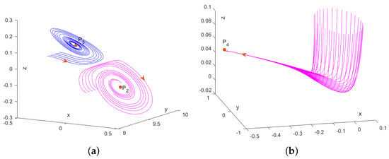
which are equivalent to $c\left(b+c\right)>1$ and $b\left(1-bc\right)\left(2ac+3\right)+b{c}^3\left(b+c\right)-2c>0.$ We notice that (6) are satisfied at least for $\alpha >0$ sufficiently small and $c^2>1.$ The results are summarized in the next Theorem 4. The attractors $P_2$ and $P_3$ with orbits converging to them are illustrated in Figure 1.

Figure 1. (a) Orbits around the attractors $P_2$ and $P_3$ in the system (3) projected in the $xyz$ space. The parameters are $a=9,$ $b=0.1,$ $c=2,$ $m=d=-1.$ The starting points for $P_2$ are $(0.2,9+i/2,-0.1,0.05),$ while for $P_3$ they are $(-0.2,9+i/2,0.1,0.05),$ for $i=0,1,2,3,4$. (b) Orbits around the attractor $P_4$ for $a=b=1,$ $c=10,$ $m=0.1$ and $d=-0.2$.

Theorem 4.

Assume $\alpha >0.$ Then, $P_2$ and $P_3$ are attractors if (6) is satisfied and ${\lambda }_4^{P_2}<0$ for $P_2,$ respectively, ${\lambda }_4^{P_3}<0$ for $P_3.$ In the other cases with ${\lambda }_4^{P_{2,3}}\ne 0,$ $P_2$ and $P_3$ are saddles.

The local behavior of the system (3) at $P_4.$ The characteristic polynomial at $P_4$ is

$$S\left(\lambda \right)={\lambda }^4+m_3{\lambda }^3+m_2{\lambda }^2+m_1\lambda +m_0,$$

where $m_3=a+b+c-\frac{1}{b}+\frac{m^2}{b{d}^2},$ $m_2=-\frac{c}{b}\alpha +\frac{m_0}{bc}+\frac{3b+c}{b{d}^2}{m}^2-2b{\beta }_1,$ $m_1=-c\frac{b+m}{b}\alpha +\frac{1}{c}{m}_0+c{m}^2\frac{3b+m}{b{d}^2}$ and $m_0=cm\frac{m^2-d^2\alpha }{d^2};$ $\alpha =\frac{1}{c}\left(c-b-abc\right)$ and ${\beta }_1=\frac{1}{2b}\left(1-ab-bc\right).$

Remark 4.

Denote by ${\beta }_2=bc+bm+cm$ and ${\beta }_3=b+c+m.$ Then $m_1$ and $m_2$ can be written in the forms

$$m_1=a{\beta }_2+N_1\mathrm{and}{m}_2=a{\beta }_3+N_2,$$

(7)

where $N_1=m^2\frac{2bc+{\beta }_2}{b{d}^2}+\left(b-c\right)\frac{{\beta }_2}{bc}$ and $N_2=m^2\frac{2b+{\beta }_3}{b{d}^2}+\frac{1}{bc}\left(b-c\right)m+\frac{c}{b}\left(b^2-1\right).$

For $c>0$ arbitrary fixed, define the following curves lying in the $ba-$parametric plane: $A=\left\{\left(b,a\right),\alpha =0,b>0\right\},$ $H=\left\{\left(b,a\right),{\beta }_1=0,b>0\right\},$ $S_2=\left\{\left(b,a\right),s_2=0,b>0\right\},$ $S_3=\left\{\left(b,a\right),s_3=0,b>0\right\},$ $L_1=\left\{\left(b,a\right),{\lambda }_4^{P_2}=0,b>0\right\},$ $L_2=\left\{\left(b,a\right),{\lambda }_4^{P_3}=0,b>0\right\}$ and $M_i=\left\{\left(b,a\right),m_i=0,b>0\right\},$ $i=1,2,3.$ Notice that b corresponds to the $x$-axis, while a to the $y$-axis, and all curves are included in the region $b>0.$

Theorem 5.

If $m_0<0,$ then $P_4$ is a saddle. Assume $m_0>0.$ Then,

(a) 

$P_4$ is a saddle or an attractor for all $d>0$ and $m\ne 0.$

(b) 

$P_4$ is an attractor if and only if $m_3>0,$ $k_0=m_3{m}_2-m_1>0$ and $k_1=\left(m_3{m}_2-m_1\right)m_1-m_3^2{m}_0>0.$ In particular, if $\alpha <0,$ ${\beta }_1<0,$ $b\left(b+c\right)\left(a+b\right)>c$ and $m>0$ sufficiently small, $P_4$ is an attractor, as shown in Figure 1.

Proof. 

It is clear that $P_4$ is a saddle if $m_0<0,$ since the product of its eigenvalues is negative.

(a)

Let further be $m_0>0.$ Assume first $m>0,$ thus, $m^2>\alpha d^2.$ It is clear that $m_1>0$ if $\alpha \le 0,$ thus,

$$E_2={\lambda }_1{\lambda }_2\left({\lambda }_3+{\lambda }_4\right)+{\lambda }_2{\lambda }_3{\lambda }_4=-m_1<0.$$

Let $\alpha >0.$ Then, $m^2>\alpha d^2$ yields $m_1>2c\alpha +\frac{1}{c}{m}_0>0,$ thus, $E_2<0.$

Secondly, assume $m<0.$ Then $m^2<\alpha d^2$ and $\alpha >0$ follow from $m_0>0.$ For an arbitrary fixed $b>0,$ denote by $\left(b,a_{l_2}\right)\in L_2,$ $\left(b,a_{m_1}\right)\in M_1,$ $\left(b,a_{m_2}\right)\in M_2$ and $\left(b,a_{m_3}\right)\in M_3$ four points from the corresponding curves. Then,

$$a_{m_1}=-\frac{N_1}{{\beta }_2},a_{m_2}=-\frac{N_2}{{\beta }_3},a_{l_2}-a_{m_1}=\frac{2c{m}^2}{d^2{\beta }_2}\mathrm{and}{a}_{m_2}-a_{m_1}=N_3,$$

(8)

where $N_3=\left(1-c^2\right)\frac{b}{c{\beta }_3}+2m^2\frac{c^2-bm}{d^2{\beta }_2{\beta }_3}.$ Notice that $a_{m_3}=\frac{1}{b}-c-b-\frac{m^2}{b{d}^2}$ and $a_{l_2}=\frac{1}{b}-\frac{1}{c}-\frac{m^2}{b{d}^2}.$ More cases need to be considered further.

(a1)

Assume ${\beta }_2\le 0.$ The curve $L_2$ is given by

$$a=a_{l_2},$$

(9)

with $b>0$ and $c>0.$ One can show that $m_0>0$ is equivalent to $a<a_{l_2}.$ If ${\beta }_2=0,$ then $m_1=\frac{2b^2{c}^3}{d^2{\left(b+c\right)}^2}>0,$ thus, $E_2=-m_1<0.$ If ${\beta }_2<0,$ then, from $m_1=a{\beta }_2+N_1$ and $a<a_{l_2},$ one gets $m_1>\frac{2c}{d^2}{m}^2,$ which leads to $E_2<0.$

(a2)

Assume ${\beta }_2>0$ and $0<c\le 1.$ Then ${\beta }_3>0$ as well. Since ${\left.m_1\right|}_{L_2}=\frac{2c{m}^2}{d^2}\ne 0$ and ${\left.m_2\right|}_{M_1}=-N_3{\beta }_3\ne 0,$ it follows that $L_2\cap M_1=\varnothing$ and $M_2\cap M_1=\varnothing ;$ we denoted as usual by ${\left.m_1\right|}_{L_2}=m_1\left(b,a\right)$ for $\left(b,a\right)\in L_2.$ From (8), one get $a_{l_2}>a_{m_1}$ and $a_{m_2}>a_{m_1},$ since $N_3>0$ if $0<c\le 1.$

For $b>0,$ denote by $M_1^{+}=\left\{\left(b,a\right),m_1>0,m_0\ge 0\right\}$ and $M_1^{-}=\{\left(b,a\right),m_1\le 0,$ $m_0\ge 0\},$ the two regions from $m_0\ge 0$ corresponding to $m_1>0,$ respectively, $m_1\le 0.$ Then $E_2=-m_1<0$ on the region $M_1^{+}.$ Notice that $L_2\subset M_1^{+},$ because ${\left.m_1\right|}_{L_2}=\frac{2c{m}^2}{d^2}>0$ and $L_2\cap M_1=\varnothing .$

If $m_1\le 0,$ which is equivalent to $a\le a_{m_1},$ one can show

$$m_2\le -N_3{\beta }_3<0,$$

whenever $0<c\le 1.$ It follows that

$$E_3={\lambda }_1\left({\lambda }_2+{\lambda }_3+{\lambda }_4\right)+{\lambda }_2\left({\lambda }_3+{\lambda }_4\right)+{\lambda }_3{\lambda }_4=m_2<0,$$

on $M_1^{-}.$ Therefore, $E_2<0$ or $E_3<0$ on $m_0>0,$ whenever ${\beta }_2>0$ and $0<c\le 1.$

(a3)

Assume ${\beta }_2>0$ and $c>1,$ thus, ${\beta }_3>0.$ Since

$${\left.m_1\right|}_{L_2}=\frac{2c{m}^2}{d^2}\ne 0,{\left.m_2\right|}_{L_2}>\frac{b}{c}\left(c^2-1\right)\ne 0\mathrm{and}{\left.m_3\right|}_{L_2}=b+c-\frac{1}{c}\ne 0,$$

it follows that $L_2\cap M_1=\varnothing ,$ $L_2\cap M_2=\varnothing$ and $L_2\cap M_3=\varnothing .$ Notice that $a_{l_2}-a_{m_2}=\frac{b{d}^2\left(c^2-1\right)+2c{m}^2}{c{d}^2{\beta }_3}>0.$

In the region $b>0,$ denote by $M_2^{+}=\left\{\left(b,a\right),m_2\ge 0,m_0\ge 0\right\}$ and $M_2^{-}=\left\{\left(b,a\right),m_2<0,m_0\ge 0\right\}.$ Then $E_3=m_2<0$ on the region $M_2^{-}.$ Notice that $L_2\subset M_2^{+},$ because ${\left.m_2\right|}_{L_2}>\frac{b}{c}\left(c^2-1\right)>0$ and $L_2\cap M_2=\varnothing .$

Assume further $m_2\ge 0.$ If $m_1>0,$ then $E_2=-m_1<0.$ It remains the case $m_1\le 0.$ We notice that $M_2$ may intersect $M_1$ in the region $m_0\ge 0,$ since

$${\left.m_2\right|}_{M_1}=2m^2\frac{bm-c^2}{d^2{\beta }_2}+\frac{b}{c}\left(c^2-1\right),$$

may be zero. The inequalities $m_2\ge 0$ and $m_1\le 0$ yield $-\frac{N_2}{{\beta }_3}\le a\le -\frac{N_1}{{\beta }_2},$ thus, $N_2{\beta }_2>N_1{\beta }_3,$ which, in turns, leads to

$$\frac{m^2}{d^2}<\frac{{\beta }_{2}b\left(c^2-1\right)}{2c\left(c^2-bm\right)}.$$

(10)

Then, $-\frac{N_2}{{\beta }_3}\le a$ and (10) yield

$$m_3>\frac{-bcm\left(b+c\right)+c^2\left(c^2-1\right)+bc+mb}{c\left(c^2-bm\right)},$$

which implies $m_3>0,$ because $bc+mb>-mc>0$ follows from ${\beta }_2>0$ and $m<0.$ Therefore,

$$E_4={\lambda }_1+{\lambda }_2+{\lambda }_3+{\lambda }_4=-m_3<0.$$

It follows that, $E_2<0$ or $E_3<0$ or $E_4<0$ whenever $m_0>0,$ if $c>0,$ $d>0$ and $m\ne 0,$ which, in turn, imply that at least one eigenvalue ${\lambda }_i$ has $Re\left({\lambda }_i\right)<0.$ This confirms the proof.

(b)

The result follows from Routh–Hurwitz conditions for $S\left(\lambda \right),$ which are $m_0>0,$ $m_3>0,$ $m_3{m}_2>m_1$ and $k_1>0.$ For the particular case, we write the expression $k_1$ as a polynomial in $m,$

$$k_1\left(m\right)=\sum _{i=1}^8{c}_i^{\prime }{m}^i+\alpha {\beta }_1\left(b\left(b+c\right)\left(a+b\right)-c\right)\frac{2c}{b}$$

for some coefficients $c_i^{\prime },$ thus, $k_1>0.$ The condition $m_3{m}_2>m_1$ follows from $k_1>0$ and $m_1>0.$

□

Example 1.

The equilibrium point $P_4$ does not exist in the 3D model. This happens due to the control function $u\left(t\right)$, defined by the two constraints in the new 4D model. When $P_4$ is an attractor and $P_4\in \Sigma$, the three state variables, namely the real interest rate $x=x\left(t\right)$, the investment demand $y=y\left(t\right)$ and the inflation rate $z=z\left(t\right)$, can be stabilized at least locally around three fixed values $\frac{m}{d},$ $\frac{d^2-m^2}{b{d}^2}$ and $-\frac{m}{cd},$ respectively, which are economically relevant if $md<0$ and $d^2>m^2.$ This scenario does not arise in the 3D model since $P_4$ is not a steady state of the model.

3. Bifurcation Diagrams

Denote by R the region

$$R=\left\{\left(b,a\right),b\ge 0\right\}.$$

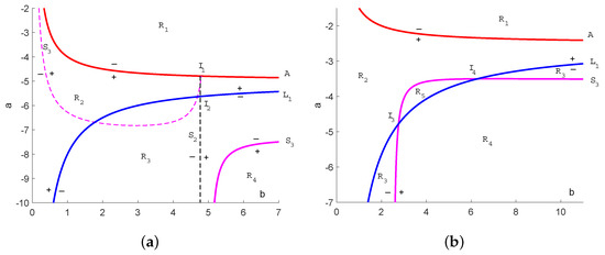
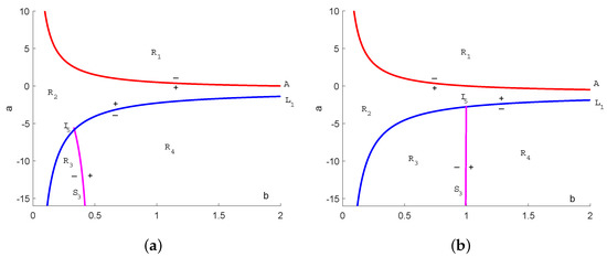
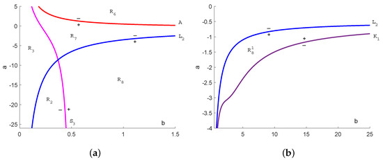
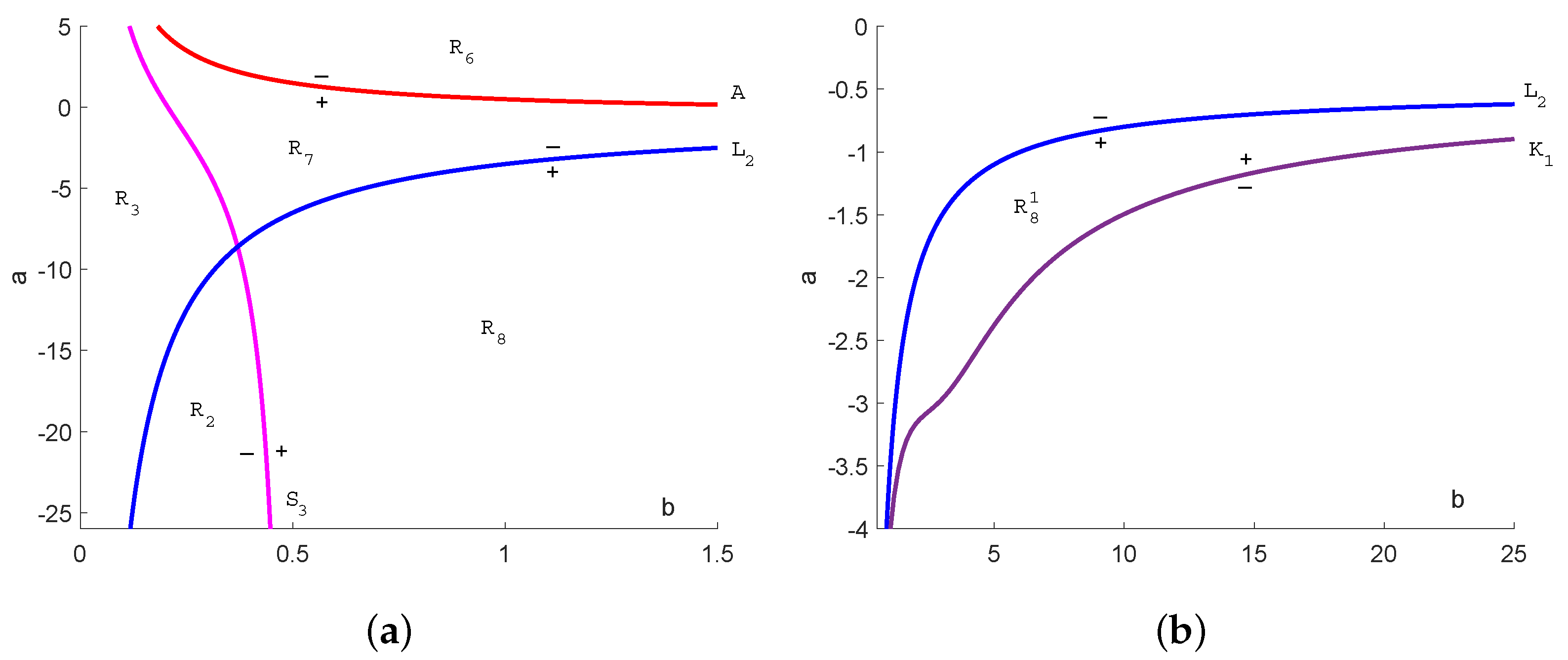
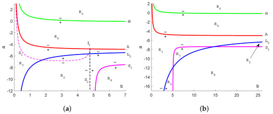
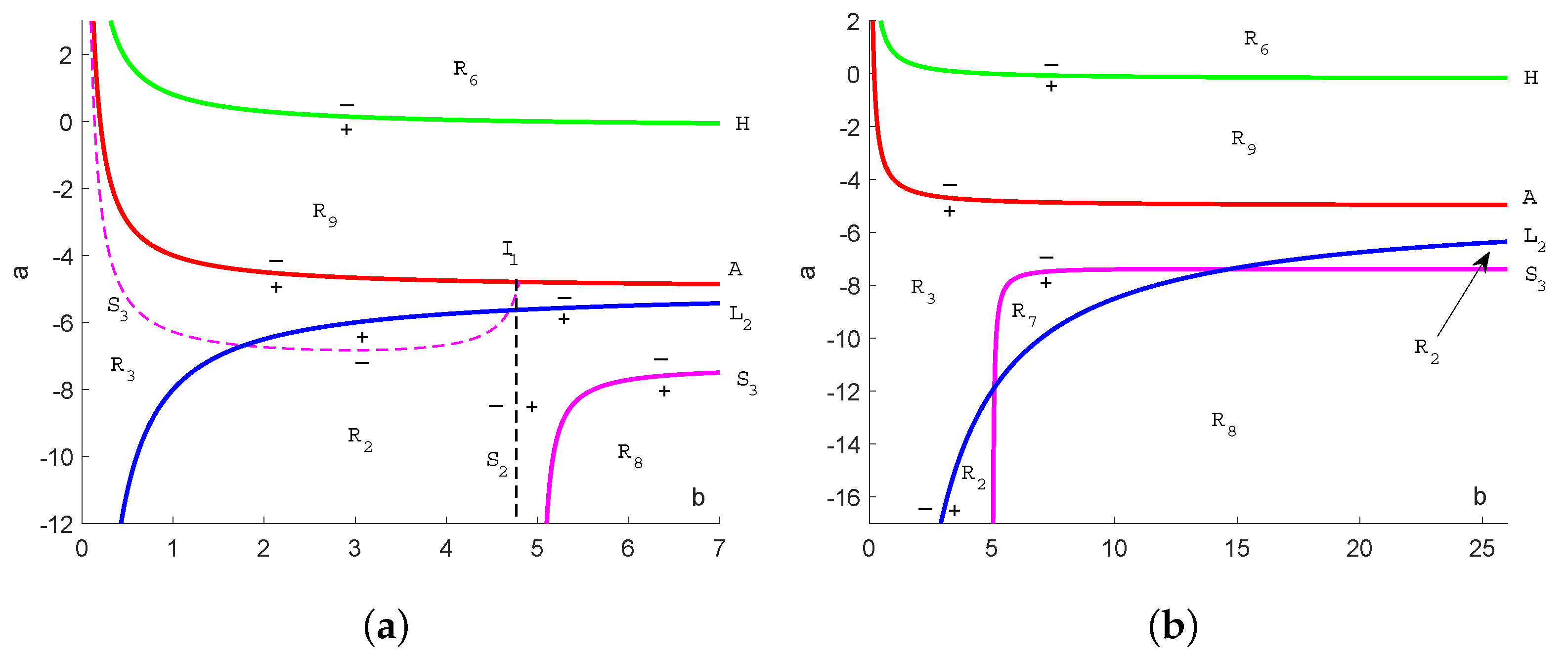
The curve A has a unique branch of the form $a=\frac{1}{b}-\frac{1}{c}$ lying in $R,$ for all $c>0$ arbitrary fixed, which splits the region R into two parts: $\alpha >0$ in the region from R that contains the origin $\left(0,0\right),$ and $\alpha <0$ in the other region, as shown in Figure 2, Figure 3, Figure 4 and Figure 5.

Figure 2. Bifurcation diagrams of the system (3) for $0<c<1$ and (a) $0<m<c_{0}d$, respectively, (b) $m>c_{0}d>0$, where $c_0=\frac{c+1}{c\sqrt{2}}\sqrt{1-c^2}$.

Figure 3. Bifurcation diagrams of the system (3) for $m>0,$ $d>0$ and (a) $c>1$, respectively, (b) $c=1$.

Figure 4. Bifurcation diagrams of the system (3) for $m<0,$ $d>0$ and $c>1,$ (a,b). A region $R_8^1$ where $P_4$ is an attractor is presented in (b).

Figure 5. Bifurcation diagrams of the system (3) for $0<c<1,$ $d>0$ and (a) $-c_{0}d<m<0$, respectively, (b) $m<-c_{0}d<0$.

$S_2$ is the vertical line $b=\frac{1}{c}-c,$ thus, $s_2<0$ on the left of $S_2$ and $s_2>0$ on the right of $S_2,$ for all $c>0$ arbitrary fixed. If $c=1,$ $s_2=b.$ If $c>1,$ the curve $S_2$ lies on $b<0,$ thus, it is outside the region of interest. However, the sign of $s_2$ is important if $c>1$ as well.

If $c\ne 1,$ the curve $S_3$ has in R two branches asymptotically to the vertical line $b=\frac{1}{c}$ (on the left and right of the line) given by $s_3=2b\frac{1-bc}{c}a+\left(c-\frac{3}{c}\right)b^2+\left(\frac{3}{c^2}+c^2\right)b-\frac{2}{c}=0.$ Notice that $s_3=\frac{c^2-1}{c}\ne 0$ if $b=\frac{1}{c}.$ It follows that $s_3<0$ in the region from R that contains $(0,0).$ The sign of $s_3$ changes when $\left(b,a\right)$ crosses a branch of $S_3,$ as shown in Figure 2, Figure 3, Figure 4 and Figure 5. Notice that a branch of the curve $S_3$ may lie on $\alpha <0,$ especially if $c>1,$ and this branch is not taken into account (it is not depicted in Figure 3 and Figure 4) because $P_{2,3}$ do not exist on $\alpha <0.$

If $c=1,$ then $s_3=2\left(1-b\right)\left(b+ab-1\right),$ thus, $S_3$ has two branches in R as well: one is the vertical line $b=1$ and the other is the curve $A,$ as shown in Figure 3b. It is clear that $s_3<0$ in the region from R that contains $(0,0).$

If $0<c<1,$ the curves $A,$ $S_2$ and $S_3$ intersect at the same point $I_1=\left(b_1,a_1\right),$ with $b_1=\frac{1}{c}-c>0$ and $a_1=\frac{2c^2-1}{c-c^3}.$ If in addition $md>0,$ then $L_1\cap S_2=\left\{I_2\right\},$ $I_2=\left(b_2,a_2\right),$ where $b_2=b_1$ and $a_2=a_1-\frac{m^{2}c}{d^2\left(1-c^2\right)},$ thus, $a_2<a_1.$ If $md<0,$ then $L_2\cap S_2=\left\{I_2\right\}.$

Since $m_0=cm\frac{m^2-d^2\alpha }{d^2},$ ${\lambda }_4^{P_2}=m-d\sqrt{\alpha }$ and ${\lambda }_4^{P_3}=m+d\sqrt{\alpha },$ by Theorem 5, the curves $L_1:{\lambda }_4^{P_2}=0$ and $L_2:{\lambda }_4^{P_3}=0$ devide the region R into two disjoint subregions (on the left and right of $L_1$, and the same for $L_2$), as shown in Figure 2, Figure 3, Figure 4 and Figure 5. On one subregion $P_4$ is a saddle, while on the other $P_4$ is a saddle or an attractor.

The following theorem clarifies the intersection of the bifurcation curves $L_1$ and $S_3.$ Since ${\lambda }_4^{P_2}$ has constant sign on $\alpha >0$ if $md<0,$ only the case $md>0$ is needed. We assume further $m>0$ and $d>0.$ The case $m<0$ and $d<0$ is similar.

Theorem 6.

Assume $m>0$ and $d>0.$ The following assertions are true.

(1) 

If $0<c<1$ and $b>\frac{1}{c},$ the intersection $L_1\cap S_3$ on $\alpha >0$ has zero points if $0<m<d{c}_0,$ one point if $m=d{c}_0$, respectively, two points if $m>d{c}_0,$ where $c_0=\frac{c+1}{c\sqrt{2}}\sqrt{1-c^2}.$

(2) 

If $0<c<1$ and $0<b\le \frac{1}{c},$ then either $s_2<0$ or $s_3<0$ on $\alpha >0.$

(3) 

If $c\ge 1,$ the intersection $L_1\cap S_3$ has a single point on $\alpha >0$ and $b>0.$

Proof. 

Since ${\lambda }_4^{P_2}=m-d\sqrt{\alpha },$ the curve $L_1$ is defined only on $\alpha >0$ and is given by $a=\frac{1}{b}-\frac{1}{c}-\frac{m^2}{b{d}^2},$ with $b>0.$ The intersection $L_1\cap S_3$ satisfies $s_3=0$ and ${\lambda }_4^{P_2}=0,$ which lead to an equation in b of the form

$$\left(c-\frac{1}{c}\right)b^2+\left(\frac{2m^2}{d^2}+\frac{1}{c^2}+c^2-2\right)b-\frac{2m^2}{c{d}^2}=0.$$

(11)

(1)

By $w=b-\frac{1}{c},$ (11) reads $p_0{w}^2+p_{1}w+p_0=0,$ where $p_0=c-\frac{1}{c}$ and $p_1=\frac{2m^2}{d^2}-\frac{1}{c^2}+c^2.$ Its roots $w_{1,2}$ satisfy $w_1{w}_2=1.$ Thus, $w_1>0$ and $w_2>0$ iff $w_1+w_2>0$ and $\mathsf{\Delta }>0$ (the discriminant). Since $p_0<0,$ the inequalities lead to $p_1>0$ and $\mathsf{\Delta }=\left(p_1-2p_0\right)\left(p_1+2p_0\right)>0,$ that is, $p_1>0$ and $p_1+2p_0>0.$ However, $p_1+2p_0=2\left(\frac{m^2}{d^2}-c_0^2\right)>0,$ where $c_0=\frac{c+1}{c\sqrt{2}}\sqrt{1-c^2}>0,$ and $m>0,$ lead to $m>d{c}_0.$ Moreover, $p_1+2p_0>0$ leads to $\frac{2m^2}{d^2}>2c_0^2>\frac{1}{c^2}-c^2>0,$ which, in turn, leads to $p_1>0.$ Therefore, $w_1>0$ and $w_2>0$ iff $m>d{c}_0.$ In this case $L_1\cap S_3=\left\{I_3,I_4\right\},$ where $I_i=\left(b_i,a_i\right),$ $a_i=\frac{1}{b_i}-\frac{1}{c}-\frac{m^2}{b_i{d}^2},$ $i=3,4$, respectively, $b_3=w_1+\frac{1}{c}$ and $b_4=w_2+\frac{1}{c}.$ It is clear that $I_3=I_4$ if $m=d{c}_0.$ If $0<m<d{c}_0$ and $p_1>0,$ then $\mathsf{\Delta }<0,$ thus $L_1\cap S_3$ is the empty set.

(2)

If $0<b<\frac{1}{c}-c,$ then $s_2<0.$ If $b=\frac{1}{c}-c,$ then $s_2=0$ and $s_3=-2c\alpha <0$ on $\alpha >0,$ while, $s_3=\frac{c^2-1}{c}<0$ if $b=\frac{1}{c}.$ Let $\frac{1}{c}-c<b<\frac{1}{c}$ and $\alpha >0.$ Then $s_2>0$ and

$$s_3=2\alpha \frac{bc-1}{c}-\frac{b}{c}{s}_2\left(1-c^2\right)<0.$$

(3)

Assume $c>1.$ Then, the roots $b_{5,6}$ of (11) satisfy $b_5{b}_6<0,$ thus, $b_5>0$ and $b_6<0;$ notice that the discriminant of Equation (11) is positive. It follows that $L_1\cap S_3=\left\{I_5\right\},$ where $I_5=\left(b_5,a_5\right)$ and $a_5=\frac{1}{b_5}-\frac{1}{c}-\frac{m^2}{b_5{d}^2}.$ If $c=1,$ then $L_1\cap S_3=\left\{I_5\right\},$ where $I_5=\left(1,-\frac{m^2}{d^2}\right).$

The theorem is now proved. □

A similar result can be obtained for the intersection of the curve $L_2$ with $S_3.$ Since ${\lambda }_4^{P_3}=m+d\sqrt{\alpha }$ has constant sign on $\alpha >0$ if $md>0,$ only the case $md<0$ is needed. We present the result for $m<0$ and $d>0,$ while the remaining case $m>0$ and $d<0$ can be treated similarly. A proof of the next theorem can be obtained as above.

Theorem 7.

Assume $m<0$ and $d>0.$ The following assertions are true.

(1) 

If $0<c<1$ and $b>\frac{1}{c},$ the intersection $L_2\cap S_3$ on $\alpha >0$ has zero points if $-d{c}_0<m<0,$ one point if $m=-d{c}_0$, respectively, two points if $m<-d{c}_0<0.$

(2) 

If $0<c<1$ and $0<b\le \frac{1}{c},$ then either $s_2<0$ or $s_3<0$ on $\alpha >0.$

(3) 

If $c\ge 1,$ the intersection $L_2\cap S_3$ has a single point on $\alpha >0$ and $b>0.$

Remark 5.

For $d>0$ and $m\in \mathbb{R}$ we obtain:

(1) 

If $m>0$ and $d>0,$ then ${\lambda }_4^{P_3}=m+d\sqrt{\alpha }>0$ and $m_0=cm\frac{{\lambda }_4^{P_2}{\lambda }_4^{P_3}}{d^2}$ has the same sign as ${\lambda }_4^{P_2}$ on $\alpha >0,$ and $m_0>0$ if $\alpha \le 0.$ The curves $\left\{m_0=0\right\}$ and $L_1$ coincide.

(2) 

If $m<0$ and $d>0,$ then ${\lambda }_4^{P_2}=m-d\sqrt{\alpha }<0$ and $m_0$ has the same sign as ${\lambda }_4^{P_3}$ on $\alpha >0,$ and $m_0<0$ if $\alpha \le 0.$ The curve $\left\{m_0=0\right\}$ coincides to $L_2$ in this case.

Remark 6.

In the following cases, we will determine the bifurcation diagrams of the system (3) when $m>0$ and $d>0$, respectively, $m<0$ and $d>0.$ One can proceed similarly in other cases.

Case 1. Assume first $0<c<1,$ $m>0$ and $d>0.$ Notice that ${\lambda }_4^{P_3}>0,$ whenever $P_3$ exists, and $\left\{m_0=0\right\}$ coincides to $L_1.$ Based on Theorem 6, two main bifurcation diagrams arise to describe the system’s dynamics, as shown in Figure 2a,b. The bifurcation curves in the two diagrams are illustrated in Matlab: Figure 2a uses $c=0.2,$ $m=1$ and $d=0.5,$ while Figure 2b $c=0.4,$ $m=2.7$ and $d=1.$

Case 2. Assume $c>1,$ $m>0$ and $d>0.$ Then $S_2$ lies on $b<0$ and $s_2>0$ on $b>0.$ By Theorem 6, $L_1\cap S_3=\left\{I_5\right\}$ in the region $\alpha >0$ from $R.$ One can show $A\cap S_3=\varnothing$ on $b>0$ and ${\beta }_1<0$ in the region R where $\alpha <0.$ As in case 1, ${\lambda }_4^{P_3}>0$ on $\alpha >0$ and $\left\{m_0=0\right\}$ coincides to $L_1.$ In particular, if $c=1,$ then $s_2=b>0$ and $s_3=2\left(b-1\right)\alpha .$ Two main bifurcation diagrams emerge in this case, which are depicted in Figure 3a,b. The curves are illustrated for $c=2,$ $m=1$ and $d=0.6$ in Figure 3a, respectively, $c=1,$ $m=1$ and $d=0.6$ in Figure 3b.

Case 3. Assume $c>1,$ $m<0$ and $d>0.$ The curve $L_2$ is given by the same expression as $L_1.$ The curve $\left\{m_0=0\right\}$ coincides to $L_2$ in this case; ${\lambda }_4^{P_2}<0$ whenever $P_2$ exists. Furthermore, $sign\left(m_0\right)=sign\left({\lambda }_4^{P_3}\right)$ on $\alpha >0$ and $m_0<0$ if $\alpha \le 0,$ respectively, ${\beta }_1<0$ in the region R where $\alpha <0.$ Using Theorem 7, a bifurcation diagram is presented in Figure 4a. Figure 4b presents a region $R_8^1$ where $P_4$ is an attractor, in a typical case $m=-1,$ $d=0.5$ and $c=2.$ The strip $R_8^1$ is quite large, it extends to infinity along the horizontal axis when $b>0$ is large. We denoted by $K_1$ the curve $\left\{\left(b,a\right),k_1=0\right\}.$

Case 4. Assume $0<c<1,$ $m<0$ and $d>0,$ thus, ${\lambda }_4^{P_2}<0$ if $\alpha >0.$ By Theorem 7, two main bifurcation diagrams arise to describe the system’s dynamics, as shown in Figure 5a,b. Figure 5a is illustrated for $c=0.2,$ $m=-1$ and $d=0.5,$ while Figure 5b for $c=0.2,$ $m=-3$ and $d=0.5.$

Remark 7.

The type of the equilibria $P_1,$ $P_{2,3}$ and $P_4$ as they appear in different regions from the above bifurcation diagrams presented in Figure 2, Figure 3, Figure 4 and Figure 5, are described in Table 1.

Table 1. The type of the equilibria $P_1,$ $P_2,$ $P_3$ and $P_4$ on different regions from bifurcation diagrams; s stands for saddle, while a for attractor.

	${\mathit{R}}_1$	${\mathit{R}}_2$	${\mathit{R}}_3$	${\mathit{R}}_4$	${\mathit{R}}_5$	${\mathit{R}}_6$	${\mathit{R}}_7$	${\mathit{R}}_8$	${\mathit{R}}_9$
$P_1$	s	s	s	s	s	a	s	s	s
$P_2$	−	s	s	a	a	−	a	s	−
$P_3$	−	s	s	s	s	−	a	a	−
$P_4$	$a,s$	$a,s$	s	s	$a,s$	s	s	$a,s$	s

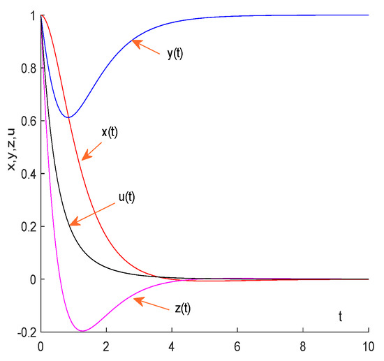
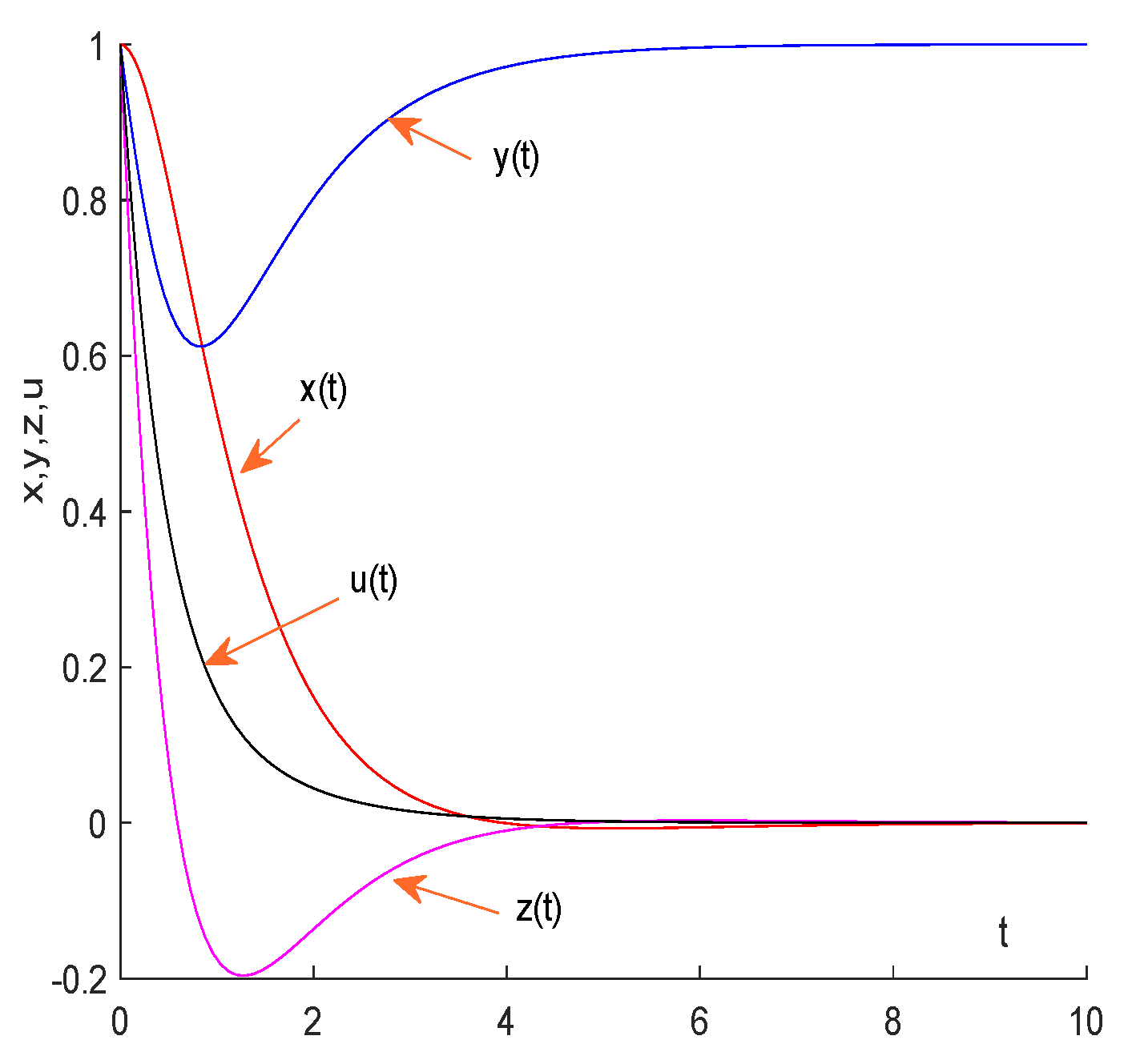
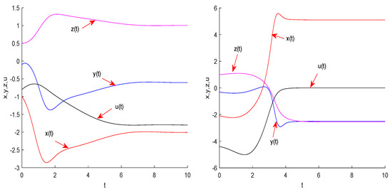
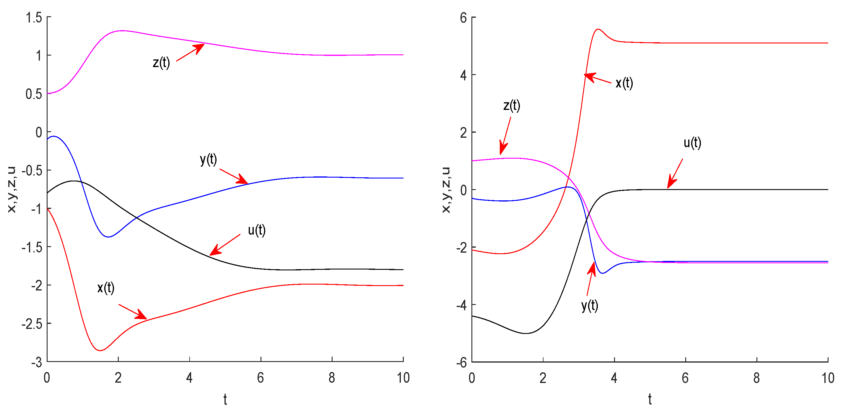
The different behavior of $P_1$ as an attractor on the region $R_6$ is presented in Figure 6, while the two possible states of $P_4$ as an attractor or saddle are depicted in Figure 7.

Figure 6. The time series of the four variables around the attractor $P_1$ in the system (3). The parameters are $a=1,$ $b=1,$ $c=2,$ $m=-1$ and $d=1.$ The starting point of these series is $(1,1,1,1)$.

Figure 7. (Left). The time series of the four variables when $P_4$ is an attractor within the region $R_8.$ The parameters are $a=-2,$ $b=5,$ $c=2,$ $m=-1,$ $d=0.5$ and $P_4(-2,-0.6,1,-1.8).$ The starting point of these series is $(-1,-0.1,-0.5,-0.8).$ One may notice that the four series converge correspondingly to the four coordinates of $P_4$ as t increases, that is, $x\left(t\right)\to -2,$ $y\left(t\right)\to -0.6,$ $z\left(t\right)\to 1,$ and $u\left(t\right)\to -1.8.$ (Right). The time series of the four variables when $P_4$ is a saddle within the region $R_8.$ The parameters are $a=-3,$ $b=10,$ $c=2,$ $m=-1,$ $d=0.5$ and $P_4(-2,-0.3,1,-4.4).$ The starting point of these series is $(-2.1,-0.3,1,-4.4).$ One may notice that the four series do not converge correspondingly to the four coordinates of $P_4$ as t increases.

4. Conclusions

An economic model based on differential equations with four variables, the real interest rate, the investment demand, the inflation rate and a control function of the system, has been investigated. The model builds upon a three-dimensional model studied earlier in [14], to which a new variable and equation related to the real interest rate are added. A qualitative analysis has been performed and more bifurcation diagrams were obtained for understanding its local behavior, which undergoes three bifurcations: transcritical, pitchfork and Hopf. Bifurcation diagrams are used to illustrate how the dynamics of the 4D system alters with the increasing value of the parameters m and c. The occurrence of Hopf bifurcation means that the system’s equilibrium points can evolve into predictable economic cycle.

The system (3) proposed in this work has three equilibrium points with economic relevance, $P_1,$ $P_3$ and $P_4,$ while the initial system studied in [14], which corresponds to $u=0$ in (3), has only one steady state with economic relevance, the point $P_1.$ Thus, the control function u proposed in this work increases the relevance of the initial model. This could lead to a better understanding of economical prediction for more complex financial phenomena and also explain complex and dynamic behaviour of various economic systems. When the control function is null, we notice that the saving amount variable a is inversely proportional with the fluctuation of the system, meaning the smaller the saving amount is, the bigger the fluctuation of the system is, so the saving amount has to keep a balance because a too small saving amount means chaotic phenomenon and a too large saving amount means a slow economy. When the control function is different from zero, the Routh-Hurwitz criterion is used to study the properties of the asymptotic stability of the economic model with control. This control function can improve the economic vigor and become a necessary condition, in order to make the economy develop well. Numerical simulations are provided using Matlab in order to illustrate the effectiveness of the proposed approaches.

References

- Angeli, D.; Rishi, A.; Rawlings, J. On average performance and stability of economic model predictive control. IEEE Trans. Autom. Control 2011, 57, 1615–1626. [Google Scholar] [CrossRef] [Scilit]
- Aizawa, H.; Ikeda, K.; Osawa, M.; Gaspar, J.M. Breaking and sustaining bifurcations in SN -invariant equidistant economy. Int. J. Bifurc. Chaos 2020, 30, 2050240. [Google Scholar] [CrossRef] [Scilit]
- Danca, M.F. Coexisting hidden and self-excited attractors in an economic model of integer or fractional order. Int. J. Bifurc. Chaos 2021, 31, 2150062. [Google Scholar] [CrossRef] [Scilit]
- Guerrini, L. Bifurcation analysis of an economic model. Int. J. Math. Anal. 2012, 6, 2779–2787. [Google Scholar]
- Medio, A.; Pireddu, M.; Zanolin, F. Chaotic dynamics for maps in one and two dimensions: A geometrical method and applications to economics. Int. J. Bifurc. Chaos 2009, 19, 3283–3309. [Google Scholar] [CrossRef] [Scilit]
- Minsky, H. Stabilizing an Unstable Economy: A Twentieth Century Fund Report; Yale University Press: London, UK, 1986. [Google Scholar]
- Romer, D. Advanced Macroeconomics; McGraw-Hill: New York, NY, USA, 2012. [Google Scholar]
- Rigatos, G. State-Space Approaches for MODELLING and control in Financial Engineering; Springer: Cham, Switzerland, 2017. [Google Scholar]
- Skovranek, T.; Podlubny, I.; Petras, I. Modeling of the national economies in state-space: A fractional calculus approach. Econ. Model. 2012, 29, 1322–1327. [Google Scholar] [CrossRef] [Scilit]
- Pelgrin, F.; Venditti, A. On the long-run fluctuations of inheritance in two-sector OLG models. J. Math. Econ. 2022, 101, 102670. [Google Scholar] [CrossRef] [Scilit]
- Ye, R.; Li, X.; Ye, Y.; Zhang, B. DynamicNet: A time-variant ODE network for multi-step wind speed prediction. Neural Netw. 2022, 152, 118–139. [Google Scholar] [CrossRef] [Scilit] [PubMed]
- Bai, J.; Wang, X.; Wang, J. An epidemic-economic model for COVID-19. Math. Biosci. Eng. 2022, 19, 9658–9696. [Google Scholar] [CrossRef] [Scilit] [PubMed]
- Rigatos, G.; Siano, P.; Ghosh, T.; Sarno, D. A nonlinear optimal control approach to stabilization of a macroeconomic development model. Quant. Financ. Econ. 2018, 2, 373–387. [Google Scholar] [CrossRef] [Scilit]
- Ma, J.; Chen, Y. Study for the bifurcation topological structure and the global complicated character of a kind of nonlinear finance system. Appl. Math. Mech. 2001, 22, 1240–1251. [Google Scholar] [CrossRef] [Scilit]
- Chen, W.C. Nonlinear dynamics and chaos in a fractional-order financial system. Chaos Solitons Fractals 2008, 36, 1305–1314. [Google Scholar] [CrossRef] [Scilit]
- Zhen, W.; Xia, H.; Guodong, S. Analysis of nonlinear dynamics and chaos in a fractional order financial system with time delay. Comput. Math. Appl. 2011, 62, 1531–1539. [Google Scholar]
- Jajarmi, A.; Hajipour, M.; Baleanu, D. New aspects of the adaptive synchronization and hyperchaos suppression of a financial model. Chaos Solitons Fractals 2017, 99, 285–296. [Google Scholar] [CrossRef] [Scilit]
- Alidousti, J.; Ghahfarokhi, M.M. Stability and bifurcation for time delay fractional predator prey system by incorporating the dispersal of prey. Appl. Math. Model. 2019, 72, 385–402. [Google Scholar] [CrossRef] [Scilit]
- Alidousti, J. Stability and bifurcation analysis for a fractional prey-predator scavenger model. Appl. Math. Model. 2020, 81, 342–355. [Google Scholar] [CrossRef] [Scilit]
- Huang, C.; Wang, J.; Chen, X.; Cao, J. Bifurcations in a fractional-order BAM neural network with four different delays. Neural Netw. 2021, 141, 344–354. [Google Scholar] [CrossRef] [Scilit] [PubMed]
- Huang, C.; Liu, H.; Chen, X.; Zhang, M.; Ding, L.; Cao, J.; Alsaedi, A. Dynamic optimal control of enhancing feedback treatment for a delayed fractional order predator-prey model. Phys. A Stat. Mech. Appl. 2020, 554, 124136. [Google Scholar] [CrossRef] [Scilit]
- Xu, C.; Liu, Z.; Liao, M.; Yao, L. Theoretical analysis and computer simulations of a fractional order bank data model incorporating two unequal time delays. Expert Syst. Appl. 2022, 199, 116859. [Google Scholar] [CrossRef] [Scilit]
- Perko, L. Differential Equations and Dynamical Systems, 3rd ed.; Springer: New York, NY, USA, 2001. [Google Scholar]
- Kuznetsov, Y.A. Elements of Applied Bifurcation Theory, 3rd ed.; Springer: New York, NY, USA, 2004. [Google Scholar]
Disclaimer/Publisher’s Note: The statements, opinions and data contained in all publications are solely those of the individual author(s) and contributor(s) and not of MDPI and/or the editor(s). MDPI and/or the editor(s) disclaim responsibility for any injury to people or property resulting from any ideas, methods, instructions or products referred to in the content. |
© 2023 by the authors. Licensee MDPI, Basel, Switzerland. This article is an open access article distributed under the terms and conditions of the Creative Commons Attribution (CC BY) license (https://creativecommons.org/licenses/by/4.0/).