The Specific Behavior of Economic Agents with Heterogeneous Expectations in the New Keynesian Model with Rigid Prices and Wages

Abstract

The purpose and scientific novelty of this work is to analyze the changes and features of economic agents’ behavior when incorporating wage rigidity into a new Keynesian model under cognitive constraints of agents. The working hypothesis is the assumption that the forecasting of the output gap, inflation of prices and wages occurs with the help of fundamentalist and extrapolation rules. The first rule is based on forecasting the variables under study on the basis of their stationary values. The second rule is based on extrapolation of the latest available data on inflation and the output gap. The weight shares of agents applying these heuristic rules change endogenously, which is the source of endogenous waves of optimism and pessimism. An analysis of the impulse responses of interest rate and technology shocks suggests that a more flexible economy (an economy with flexible wages and rigid prices) is less prone to a spike in the economic cycle caused by waves of optimism and pessimism than a more rigid economy (an economy with rigid prices and wages) due to the inability of agents to respond immediately to exogenous disturbances in rigid conditions. Thus, these shocks cause wave effects in the economy, i.e., cyclical movements, i.e., a rigid economy will be more prone to booms and busts caused by alternating optimism and pessimism than a flexible economy. The model with an imperfect labor market is characterized by an increased concentration of vital forces at the values of 0 and 1, as well as in the mid-distribution compared to the base model. This feature provides a key explanation for the abnormal dynamics of the evolution of variables in this model. It is concluded that the difference between the degree of optimism and pessimism in the base model and in the model with rigid wages and prices is the full trust of agents in the central bank in targeting wage inflation in the absence of the stabilization of this inflation by the bank.

1. Introduction

In recent decades, theoretical contributions to macroeconomics have mainly been based on dynamic stochastic general equilibrium models (DSGE models) with rational expectations, where a representative agent is able to understand the complexity of the underlying mathematical model [1,2,3]. The advantage of these models is, firstly, that they have microeconomic justifications, that is, it is assumed that consumers maximize the expected discounted sum of utility function values, and producers maximize their profits in dynamics. This implies that macroeconomic equations must be derived from this optimizing behavior of consumers and producers.

Secondly, it is assumed that consumers and producers have rational expectations, i.e., make predictions using all available information, including information embedded in the model [4,5,6]. This assumption also means that agents know the true statistical distribution of all shocks hitting the economy. They then use this information in their optimization procedure. Because consumers and all producers share the same information, we can take only one representative consumer and one representative producer and model the entire economy. There is no heterogeneity in the behavior of consumers and producers.

Thirdly, there is a new Keynesian feature; it is assumed that prices are not set instantly. This feature contrasts with the new classical model (sometimes also called the “real business cycle” model), which assumes ideal price flexibility.

The global financial crisis, however, has shown that agents are not fully aware of the complexity of the world in which they live. Instead, their cognitive capacity seems to be very limited. Numerous data and pieces of evidence indicate the importance of including heterogeneous expectations in general equilibrium models [7,8,9,10,11].

It should be noted that the DSGE-stylized model with rational expectations cannot capture the typical features of real business cycle movement, i.e., the correlation between subsequent observations of the output gap (auto-correlation) and the occurrence of large booms and busts (fat-tailed distributions of variables) without incorporating unsubstantiated assumptions. Therefore, it is necessary to develop macroeconomic models that do not impose implausible cognitive abilities on individual agents.

The vast majority of research is devoted to the analysis of behavioral models with rigid prices and flexible wages (references to these studies, both theoretical and using laboratory experiments, are given in the literature review). Therefore, it is of interest to study the influence of wage rigidity (along with price rigidity) on the behavior of agents with irrational expectations.

The integrative value of the paper, on the one hand, lies in the fact that, unlike behavioral models studied recently [8,12,13,14,15,16], the model proposed in the publication has imperfections in the form of wage rigidity, which cannot but impose changes in the behavior of agents in the context of their animal spirits and changes in the response of macro variables to impulse responses. In particular, the paper shows that incorporating wage rigidity in the model under study as compared to the baseline model leads to changes in the monetary policy of the authorities. On the other hand, the integrative value of the paper lies in its undeniable contribution to the analysis of the impact of price rigidity on monetary and fiscal policy changes in New Keynesian models. As noted above, all studies in this area refer to models with rational expectations of agents [17,18,19] (the authors cite references to the most recent work in this field). The incremental knowledge in the proposed paper compared to those cited is that households offer differential labor. This imperfect interchangeability between types of labor gives them some market power and allows researchers to reflect on the consequences of wage rigidity.

Thus, the purpose and scientific novelty of the work is to analyze the changes and features of the economic agents’ behavior when incorporating labor market imperfections (wage rigidity) into a new Keynesian model compared to a model with flexible wages and rigid prices under cognitive constraints of agents. At the same time, the formation of expectations in these models will be considered as an interactive process between fundamentalist agents, who predict the output gap and inflation of prices and wages based on their stationary values, and agents who use the forecasting rule based on the extrapolation of the latest available data on inflation and the output gap.

Literature Review

The heterogeneity of the agents as well as their cognitive abilities have been verified using surveys as well as research data [20,21,22,23,24,25]. Researchers have only recently begun to incorporate elements of behavioral economics into dynamic macromodels [26]. It is worth noting that some studies point out that the linearity inherent in DSGE models with rational expectations makes them of limited suitability for monetary and fiscal policy analysis. The use of macroeconomic models that take into account the cognitive limitations of agents can improve our understanding of the economic agents’ behavior in the real world. The studies [27,28,29] consider dynamic macroeconomic models under the hypothesis that agents form expectations based on simple rules and have bounded rationality. Two types of agents are considered. The first type of agents predict the output gap and inflation based on their equilibrium (stationary) values. In the following, these agents will be referred to as fundamentalist agents. For the second type of agents, a forecasting rule is used which extrapolates the latest data on inflation and the output gap. In what follows, these agents will be referred to as extrapolator agents. De Grauwe [29] implements these heterogeneous expectations in a standard new Keynesian model with fixed prices, consisting of three equations, and shows how such a structure is able to generate endogenous waves of agents’ optimistic and pessimistic beliefs (“animal spirit”), which are closely related to the business cycle. At the same time, in the studied models, agents are ready to learn, that is, they constantly evaluate the effectiveness of their forecast. At the same time, in the models under study, agents are willing to learn, i.e., they constantly evaluate the effectiveness of their forecast, and this ability is a fundamental definition of rational behavior. Thus, the agents analyzed in these models are rational because they learn from their mistakes. To characterize such behavior, the concept of “bounded rationality” is often used, which will be used in the following research.

In addition, agents can use simpler rules (heuristics) to predict future output and inflation. It is also noted that agents’ forecasts are biased because they do not understand how inflation and the output gap are determined. At the same time, it is believed that some agents are optimistic and regularly increase the output gap and inflation, while others are pessimistic and regularly underestimate these variables.

In all publications (including those listed above) that analyze the cognitive limitations of agents, the labor market is modeled as a market of perfect competition with flexible wages. The imperfections of the labor market and their consequences, in particular, for monetary policy are not considered there. Meanwhile, a feature of models with rigid wages and prices is that the full stabilization of price inflation is no longer considered optimal [30,31]. The central bank is therefore concerned about the stability of wages and prices because fluctuations in inflation and the output gap are a source of inefficient resource allocation, making households poorer.

The distribution of heterogeneity of agents changes over time, which is confirmed by many empirical data. For example, in [32], various studies of inflation expectations show a wide, time-varying range of opinions. Results of research [23,33] confirm the time-varying distribution of agents with discrete (exogenous) predictors. The proposed model is an extension of the last listed publications, in which the ratio of fundamentalist agents and extrapolator agents, by analogy with [34], is endogenous. Additionally, this article expands publications [27,28,29] including the endogenous choice of predictors in a new Keynesian model with an imperfect labor market, which is the scientific novelty of the work.

The approach presented in this study is not the only one possible. There are now a large number of studies that use macroeconomic models with imperfect data. These studies are based on the statistical learning approach proposed in [35,36]. This approach leads to important new conclusions [37,38,39]. Nevertheless, the authors believe that this approach overloads individual agents with an excessively large set of cognitive skills that they probably do not possess in the real world.

2. Materials and Methods

2.1. Model Description

The model under study is a new Keynesian model in which nominal wages and prices are rigid. A detailed description of the model is presented in [30]. The main assumptions of the model are as follows.

Firms produce differentiable products according to a linear production function (1)

$$Y_t(i)=A_t{N}_t{(i)}^{1-\alpha }$$

(1)

where $A_t$ is the total factor productivity; $a_t\equiv \log A_t$; (1 − α) is the elasticity of output with respect to labor; $Y_t\left(i\right)$—the volume of output of the i-th product and good $\left(I\in \left[0,1\right]\right)$; $N_t\left(i\right)$ is the amount of labor expended by the i-th firm in the production of this product, defined as (2)

$$N_t(i)={\left[{\displaystyle {\int }_0^1{N}_t}{(i,j)}^{1-1/{\epsilon }_w}dj\right]}^{\frac{{\epsilon }_w}{{\epsilon }_w-1}},$$

(2)

where $N_t\left(i,j\right)$ is the number of labor resources $j \left(j\in \left[0,1\right]\right)$ used by the i-th firm. The parameter ${\epsilon }_W$ is the elasticity of substitution between different types of labor.

Firms set prices according to the Calvo approach [40,41]. Some firms $\left(1-{\theta }_p\right)$ revise prices in each period, the other part ${\theta }_p$, which does not change prices, indexes them in each period. The pricing problem for a firm that is able to update its price in period t is dynamic: the price it chooses today will affect the profits it earns both today and in the future. A firm that adjusts its price in period t solves the profit optimization problem while limiting demand for products (3)

$$Y_{t+k,t}={\left(\frac{P_t^{*}}{P_{t+k}}\right)}^{-{\epsilon }_p}{C}_{t+k},$$

(3)

for k = 0, 1, 2,…..; where $Y_{t+k,t}$—the volume of output in period t + k by firms that last adjusted their price in period t; $C_{t+k}$—volume of consumption in period t + k;${\epsilon }_p$– elasticity of substitution for differentiated goods.

The economy is populated by a unit continuum of representative j- households, $\left(j\in \left[0,1\right]\right)$, seeking to maximize the expected discounted sum of the values of the utility function and the function of time spent on labor (4)

$$\max {\tilde{E}}_0\{{\displaystyle \sum _{t=0}^{\infty }{\beta }^t}[U(C_t(j))-V(N_t(j))]\},$$

(4)

where $U(C_t(j))\equiv C_t^{1-\sigma }(j)/(1-\sigma )$—the utility function; $V(N_t(j))\equiv N_t^{1+\varphi }(j)/(1+\varphi )$—the function of time spent on labor; ${\tilde{E}}_0$—operator of boundedly rational expectations of economic agents (in this case, households); $\beta$—discount factor (0 < $\beta$ < 1), $\sigma$—parameter inverse to the elasticity of intertemporal substitution; $\varphi$—parameter inverse to the elasticity of labor supply; $N_t\left(j\right)$—the amount of labor offered by the j-household and (5)

$$C_t(j)={\left({\displaystyle \underset{0}{\overset{1}{\int }}{C}_t{(i,j)}^{1-\frac{1}{{\epsilon }_p}}di}\right)}^{\frac{{\epsilon }_p}{{\epsilon }_p-1}},$$

(5)

is the consumption index of the i-th product.

Similar to the constraints firms face when setting prices, assume that in each period only a subset $\left(1-{\theta }_w\right)$ of households, selected at random from the population, reoptimize their stated nominal wages. The other part ${\theta }_w$, which does not change wages, indexes it in each period. The wage-setting problem for households that obtain the opportunity to upgrade in period t is also dynamic: the wage one chooses today will affect the expected number of discounted utilities generated over the period over which wages remain the same.

The log-linearized system of equations of the new Keynesian model with rigid nominal wages and prices in a state of general equilibrium in accordance with [30] is presented in the following way (6)

$${\pi }_t^p=\beta {\tilde{E}}_t\left\{{\pi }_{t+1}^p\right\}+{\kappa }_p{\tilde{y}}_t+{\lambda }_p{\tilde{w}}_t+u_t{u}_t~N(0,{\sigma }_u^2)$$

(6)

$${\pi }_t^w=\beta {\tilde{E}}_t\left\{{\pi }_{t+1}^w\right\}+{\kappa }_w{\tilde{y}}_t-{\lambda }_w{\tilde{w}}_t+{\delta }_t,\hspace{1em}{\delta }_t~N(0,{\sigma }_{\delta }^2),$$

(7)

$${\tilde{y}}_t=-1/\sigma (i_t-{\tilde{E}}_t\{{\pi }_{t+1}^p\}-r_t^n)+{\tilde{E}}_t\left\{{\tilde{y}}_{t+1}\right\}+{\mu }_t,\hspace{1em}{\mu }_t~N(0,{\sigma }_{\mu }^2),$$

(8)

$${\tilde{w}}_t={\tilde{w}}_{t-1}+{\pi }_t^w-{\pi }_t^p-\mathsf{\Delta }{w}_t^n,$$

(9)

$$i_t=\rho i_{t-1}+(1-\rho )({\varphi }_{\pi }{\pi }_t^p+{\varphi }_w{\pi }_t^w+{\varphi }_y{\tilde{y}}_t)+{\eta }_t,{\eta }_t~N(0,{\sigma }_{\eta }^2),$$

(10)

where $\widetilde{E_t}$—expectation operator characterizing the bounded rationality of agents.

It should be noted that the system of Equation (6) is written in the variables of the output gap $\widetilde{y_t}=y_t-y_t^n$ and the real wage gap $\widetilde{w_t}=w_t-w_t^n$, where the natural level of output is determined under flexible prices and wages. The natural wage level $w_t^n$ is determined similarly (in the absence of nominal rigidities).

Thus, the system of equations includes Equation (6) for price inflation ${\pi }_t^p$; Equation (7) for wage inflation ${\pi }_t^w$; the standard demand Equation (8) for the output gap $\widetilde{y_t}$; Equation (9) for the real wage gap $\widetilde{w_t}$; Equation (10) for the nominal interest rate $i_t$ (Taylor’s rule).

In this case, the natural level of output is determined by Formula (7). References to the definition of the parameters in Equation (6)–(12) are given in

Table 1. Values of the parameters of the system of Equation (6).

Parameters of the System of Equations	Values
${\kappa }_p$	$\frac{\alpha {\lambda }_p}{1-\alpha }$
${\kappa }_w$	${\lambda }_w(\sigma +\frac{\varphi }{1-\alpha })$
${\lambda }_p$	$\frac{(1-{\theta }_p)(1-\beta {\theta }_p)}{{\theta }_p}\frac{1-\alpha }{1-\alpha +\alpha {\epsilon }_p}$
${\lambda }_w$	$\frac{(1-{\theta }_w)(1-\beta {\theta }_w)}{{\theta }_w(1+{\epsilon }_w\varphi )}$
${\psi }_{ya}^n$	$\frac{1+\varphi }{\alpha (1-\alpha )+\varphi +\alpha }$
${\psi }_{wa}^n$	$\frac{1-\alpha {\psi }_{ya}^n}{1-\alpha }$
${\vartheta }_y^n$	$-\frac{(1-\alpha )[{\mu }_p-\log (1-\alpha )]}{(1-\alpha )\sigma +\varphi +\alpha }$

.

$$y_t^n={\psi }_{ya}^n{a}_t+{\vartheta }_y^n$$

(11)

The natural wage rate is determined by (12)

$$w_t^n=\log (1-\alpha )+{\psi }_{wa}^n{a}_t-{\mu }_p$$

(12)

where ${\mu }_p$—is the stationary value of the price premium.

In addition, in Equation (8), there is a natural level of interest rate $r_t^n$ defined as (13)

$$r_t^n=1/\beta +\sigma {\psi }_{ya}^n{\tilde{E}}_t\left\{\mathsf{\Delta }{a}_{t+1}\right\}.$$

(13)

Thus, there is a logarithm of the total factor productivity ${\eta }_t$ in Equations (11)–(13). Therefore, to the system of Equation (6) one should add the autoregressive Equation (14) for the technological factor

$$a_t={\rho }_a{a}_{t-1}+{\epsilon }_t,\hspace{1em}{\epsilon }_t~N(0,{\sigma }_{\epsilon }^2).$$

(14)

Equations (10) and (14) contain five exogenous shocks to the interest rate ${\eta }_t$, price inflation $u_t$, wage inflation ${\delta }_t$, aggregate demand ${\mu }_t$, and total factor productivity ${\epsilon }_t$.

Table 1 shows the values of the parameters of the system of Equation (6), expressed in terms of model coefficients.

Substituting the expression for the interest rate from Equation (10) into Equation (8), the expression for the real wage gap from Equation (9) into Equation (6) and (7), and the expression for the technological factor from Equation (14) into Equation (6)–(9), we obtain in matrix form (15)

$$\begin{gathered} \left[\begin{array}{ccc}1+{\lambda }_p& -{\lambda }_p& -{\kappa }_p\\ -{\lambda }_w& 1+{\lambda }_w& -{\kappa }_w\\ (1/\sigma )\rho {\varphi }_{\pi }& (1/\sigma )\rho {\varphi }_w& 1+(1/\sigma )\rho {\varphi }_y\end{array}\right]\left[\begin{array}{c}{\pi }_t^p\\ {\pi }_t^w\\ {\tilde{y}}_t\end{array}\right]=\left[\begin{array}{ccc}\beta & 0& 0\\ 0& \beta & 0\\ 1/\sigma & 0& 1\end{array}\right]\left[\begin{array}{c}{\tilde{E}}_t{\pi }_{t+1}^p\\ {\tilde{E}}_t{\pi }_{t+1}^w\\ {\tilde{E}}_t{\tilde{y}}_{t+1}\end{array}\right] \\ +\left[\begin{array}{c}{\lambda }_p\\ -{\lambda }_w\\ 0\end{array}\right]{\tilde{w}}_{t-1}+\left[\begin{array}{c}0\\ 0\\ -(1/\sigma )(1-\rho )\end{array}\right]i_{t-1}+\left[\begin{array}{c}-{\lambda }_p({\rho }_a-1)\\ {\lambda }_w({\rho }_a-1)\\ {\psi }_{ya}^n({\rho }_a-1){\rho }_a\end{array}\right]a_{t-1}+ \\ \left[\begin{array}{c}{u}_t-{\lambda }_p{\epsilon }_t\\ {\lambda }_w{\epsilon }_t+{\delta }_t\\ {\psi }_{ya}^n({\rho }_a-1){\epsilon }_t-(1/\sigma ){\eta }_t+{\mu }_t\end{array}\right], \end{gathered}$$

(15)

or

$$A{Z}_t=B{\tilde{E}}_t{Z}_{t+1‘}+b{\tilde{w}}_{t-1}+c{i}_{t-1}+d{a}_{t-1}+v_t$$

(16)

The solution for $Z_t$ is defined as:

$$Z_t=A^{-1}(B{\tilde{E}}_t{Z}_{t+1‘}+b{\tilde{w}}_{t-1}+c{i}_{t-1}+d{a}_{t-1}+v_t)$$

(17)

2.2. Formation of Boundedly Rational Expectations of the Output Gap

When describing the formation of heuristics of the studied variables by economic agents, we will follow [27,28,29]. As it was already noted in the Introduction, agents use simple rules (heuristics) to predict future output. Two types of prediction rules are assumed. The first rule can be called a “fundamentalist” one. Agents estimate a stationary equilibrium value of the output gap (which is normalized to zero) and use it to predict the future value of this variable. The second prediction rule is extrapolative. This rule does not assume that agents know the steady state output gap. Instead, they extrapolate the previous observed output gap to the future unobserved value of the variable.

The given rules are specified as follows: the fundamentalist rule is defined as follows (18)

$${\tilde{E}}_t^f{y}_{t+1}=0$$

(18)

the extrapolation rule is defined as (19)

$${\tilde{E}}_t^e{y}_{t+1}=y_{t-1}.$$

(19)

These rules are often applied in research on behavioral finance [34,42]. The simplest assumption regarding the cognitive constraints of agents is that they should only use information that they understand.

The market output gap forecast is defined as the weighted average of these two forecasts described, i.e., (20)

$${\tilde{E}}_t{y}_{t+1}={\alpha }_{f,t}{\tilde{E}}_t^f{y}_{t+1}+{\alpha }_{e,t}{\tilde{E}}_t^e{y}_{t+1},{\alpha }_{f,t}+{\alpha }_{e,t}=1,$$

(20)

where ${\alpha }_{f, t}, {\alpha }_{e, t}$ are the probabilities of agents choosing the fundamentalist or extrapolation rule, respectively.

As it was already noted, the agents in the model under study are ready to learn from their mistakes, i.e., they constantly evaluate the effectiveness of their forecast. This willingness to learn and change their behavior is the most fundamental characteristic of boundedly rational agents. In this case, the first step in their analysis is to predict the effectiveness of a particular rule, which they calculate as follows (21), (22)

$$U_{f,t}=-{\displaystyle \sum _{q=0}^{\infty }{w}_q(y_{t-q-1}}-{\tilde{E}}_{t-q-2}^f{y}_{t-q-1}{)}^2$$

(21)

$$U_{e,t}=-{\displaystyle \sum _{q=0}^{\infty }{w}_q(y_{t-q-1}}-{\tilde{E}}_{t-q-2}^e{y}_{t-q-1}{)}^2$$

(22)

where $U_{f,t},U_{e,t}$ are defined as mean square errors (MSFE) of prediction rules; $w_q$ are geometrically decreasing weights.

The $w_q$ weights decrease because agents are assumed to place less importance on mistakes made far in the past compared to mistakes made recently. The degree of forgetting plays an important role in the model under study. Assuming that the weights $w_q=(1-{\rho }_q){\rho }_q^q(0\le {\rho }_q\le 1)$ of expressions (21) and (22) can be rewritten (23), (24)

$$U_{f,t}={\rho }_q{U}_{f,t-1}-(1-{\rho }_q){(y_{t-1}-{\tilde{E}}_{t-2}^f{y}_{t-1})}^2$$

(23)

$$U_{e,t}={\rho }_q{U}_{e,t-1}-(1-{\rho }_q){(y_{t-1}-{\tilde{E}}_{t-2}^e{y}_{t-1})}^2$$

(24)

Applying discrete choice theory, the probability that an agent will use a fundamentalist prediction rule is given by (25) [34]

$${\alpha }_{f,t}=\frac{\exp (\gamma U_{f,t})}{\exp (\gamma U_{f,t})+\exp (\gamma U_{e,t})}$$

(25)

The probability of an agent using extrapolation forecasting is defined as (26)

$${\alpha }_{e,t}=\frac{\exp (\gamma U_{e,t})}{\exp (\gamma U_{f,t})+\exp (\gamma U_{e,t})}=1-{\alpha }_{f,t}$$

(26)

Equation (25) reflects the fact that as fundamentalists’ past forecasts improve relative to extrapolators, agents are more likely to choose the fundamentalist output gap rule for their future forecasts. Therefore, the likelihood that agents use the fundamentalist rule increases. Equation (26) is interpreted similarly. The parameter $\gamma$ shows “selection intensity”, i.e., the intensity of an agent’s choice of a particular heuristic, depending on past forecast performance. In the limit when $\gamma =\infty$, only one, the most efficient heuristic, will be chosen.

The above selection mechanism is a disciplinary tool introduced into the model in relation to acceptable rules of behavior. Only those rules that have passed the suitability test remain valid. The rest are weeded out. This mechanism should be understood as a learning mechanism based on “trial and error”. Agents avoid systematic errors by constantly seeking to learn from past mistakes and change their behavior. The mechanism that governs the choice of rules introduces self-organizing dynamics into the model.

2.3. Formation of Boundedly Rational Expectations of Price and Wage Inflation

Agents must also forecast price and wage inflation. As in the case of output gap forecasting, a simple heuristic is applied, where a fundamental and an extrapolation rule are used [43]. The first rule is based on the announced target inflation rate, that is, agents using the fundamentalist rule are confident in its validity and use this confidence to predict inflation. Agents have full confidence in the central bank, even though there are no rules for commitment. For agents who do not trust the announced inflation targets, extrapolation heuristics are used. Instead, they extrapolate past the observed price and wage inflation to the future unobserved value of these variables.

The fundamentalist rule will be called the “inflation targeting” rule. It consists in using the inflation target of the central bank to forecast price and wage inflation, i.e., price inflation (27)

$${\tilde{E}}_t^{tar,p}{\pi }_{t+1}={\pi }^{*},$$

(27)

and for wage inflation (28)

$${\tilde{E}}_t^{tar,w}{\pi }_{t+1}^w={\pi }^{w*},$$

(28)

where the target values ${\pi }^{*},{\pi }^{w*}$ are assumed to be zero.

The extrapolation rule for price inflation is defined as (29)

$${\tilde{E}}_t^{ext}{\pi }_{t+1}={\pi }_{t-1},$$

(29)

and for wage inflation (30)

$${\tilde{E}}_t^{ext,w}{\pi }_{t+1}^w={\pi }_{t-1}^w.$$

(30)

The market price inflation forecast is defined as the weighted average of the two forecasts, i.e., (31)

$${\tilde{E}}_t{\pi }_{t+1}={\beta }_{tar,t}{\tilde{E}}_t^{tar}{\pi }_{t+1}+{\beta }_{ext,t}{\tilde{E}}_t^{ext}{\pi }_{t+1},{\beta }_{tar,t}+{\beta }_{ext,t}=1,$$

(31)

and for wage inflation (32)

$${\tilde{E}}_t{\pi }_{t+1}^w={\beta }_{tar,t}^w{\tilde{E}}_t^{tar,w}{\pi }_{t+1}^w+{\beta }_{ext,t}^w{\tilde{E}}_t^{ext,w}{\pi }_{t+1}^w,{\beta }_{tar,t}^w+{\beta }_{ext,t}^w=1.$$

(32)

As in the case of output gap forecasting, a similar selection mechanism is applied to determine the probability that agents will trust the inflation target or that they will not (in this case, past inflation extrapolation is used) (33) and (34)

$${\beta }_{tar,t}=\frac{\exp (\gamma U_{tar,t})}{\exp (\gamma U_{tar,t})+\exp (\gamma U_{ext,t})},$$

(33)

$${\beta }_{ext,t}=\frac{\exp (\gamma U_{ext,t})}{\exp (\gamma U_{tar,t})+\exp (\gamma U_{ext,t})},$$

(34)

where $U_{tar,t}$ and $U_{ext,t}$ are the weighted average squares of past price inflation forecast errors using the fundamentalist and extrapolator rules, respectively. They are defined in the same way as in (23) and (24). For wage inflation, similar probabilities are defined as (35) and (36)

$${\beta }_{tar,t}^w=\frac{\exp (\gamma U_{tar,t}^w)}{\exp (\gamma U_{tar,t}^w)+\exp (\gamma U_{ext,t}^w)},$$

(35)

$${\beta }_{ext,t}^w=\frac{\exp (\gamma U_{ext,t}^w)}{\exp (\gamma U_{tar,t}^w)+\exp (\gamma U_{ext,t}^w)}.$$

(36)

The heuristic data for forecasting price and wage inflation can be defined as an agent’s procedure for finding out how much confidence can be placed in the central bank. If confidence in the central bank is high, the use of an inflation target yields good forecasts. However, if the inflation target does not give good forecasts, the probability that agents will use it is low.

3. Research Results and Discussion

To solve Equation (17), the model coefficients were calibrated and their values corresponded to the values of these parameters in [30]. The same coefficient values are used in the rigid price-flexible wage model being compared, which we will hereafter consider as the base model. The values of the model coefficients are given in

Table 2. Values of the coefficients of the studied model.

Coefficients *	Value
$\sigma$	1
$\varphi$	2
$\alpha$	0.4
$\beta$	0.99
${\theta }_p^{}$	0.75
${\theta }_w$	0.75
${\epsilon }_p$	6
${\epsilon }_w$	4.5
$\rho$	0.5
${\rho }_a$	0.7
${\varphi }_{\pi }$	1.5
${\varphi }_{{}_w}$	0.5
${\varphi }_y$	0.5

* The meaning of the coefficients is given in the description of the model.

. Note that the standard deviations of all shocks in Equation (17) are 0.5.

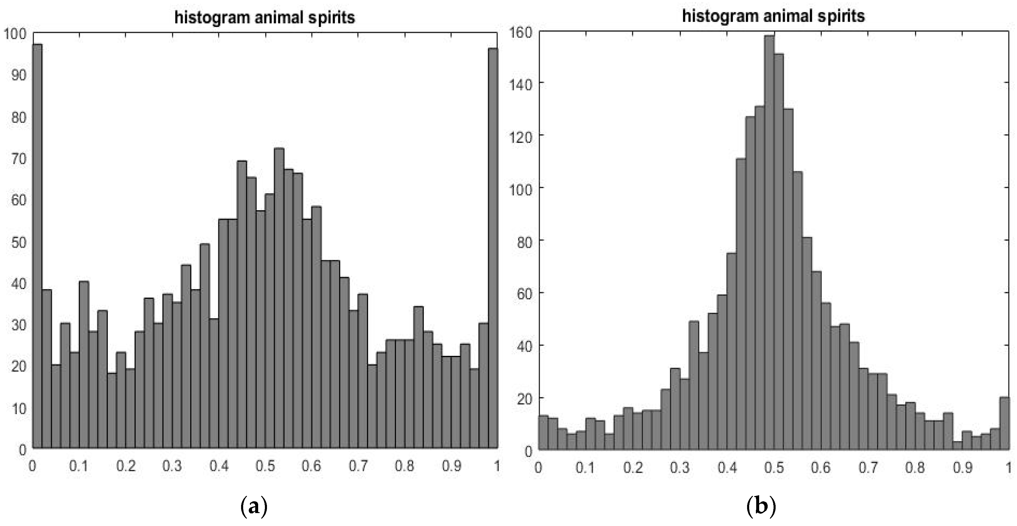
De Grauwe in his works [27,28,29] introduced a variable called the degree of animal spirit, characterizing the concentration of vitality. It shows the evolution of the number of agents that extrapolate a positive output gap. Thus, when the curve reaches 1 (Figure 1), all agents extrapolate a positive output gap and are optimists; when the curve reaches 0, no agent extrapolates a positive output gap. Such agents are pessimists. In fact, in this case, they all extract a negative output gap. Thus, the curve shows the degree of optimism and pessimism of the agents predicting the output gap.

Figure 1 shows histograms of the frequency distribution of this variable for two compared models with coefficients from Table 2. From a comparison of the histograms, it can be seen that the first model (with an imperfect labor market) is characterized by an increased concentration of vital forces at values of 0 and 1, as well as in the middle of the distribution. This feature provides a key explanation for the abnormal dynamics of variable evolution. The basic model is characterized by a lesser degree of concentration of vital forces at extreme values and in the middle of the distribution. However, the distribution of the concentration of the vital forces of this model, like the first one, has “fat tails”, which characterize the abnormality. Since the degree of optimism and pessimism of the agents of the first model is much higher than the second one, the model with an imperfect labor market is more subject to cyclical behavior compared to the base model.

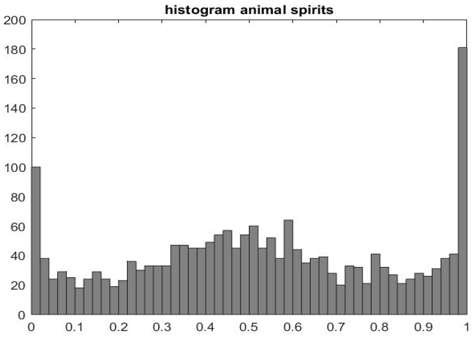
From Table 1 and Equation (8), it follows that the degree of wage rigidity depends on the parameter ${\lambda }_w$. The value of this parameter, corresponding to the values of the coefficients in Table 1, is 0.008. With an increase in the value of this parameter, the degree of wage rigidity decreases and its flexibility increases accordingly. Therefore, for an example, Figure 2 shows a histogram of the frequency distribution of the degree of animal spirits for the model under study with an imperfect labor market at ${\lambda }_w=0.1$, that is, for a model with more flexible wages compared to the model shown in Figure 1a.

The given histogram is characterized by an increased degree of agents’ optimism compared to the histogram for the base model. The degree of agents’ pessimism remained at the same level. In addition, the concentration of the vitality of agents in the middle of the distribution has decreased, and the above model with more flexible wages still reflects the abnormality of the dynamics of variables and is subject to cyclical behavior.

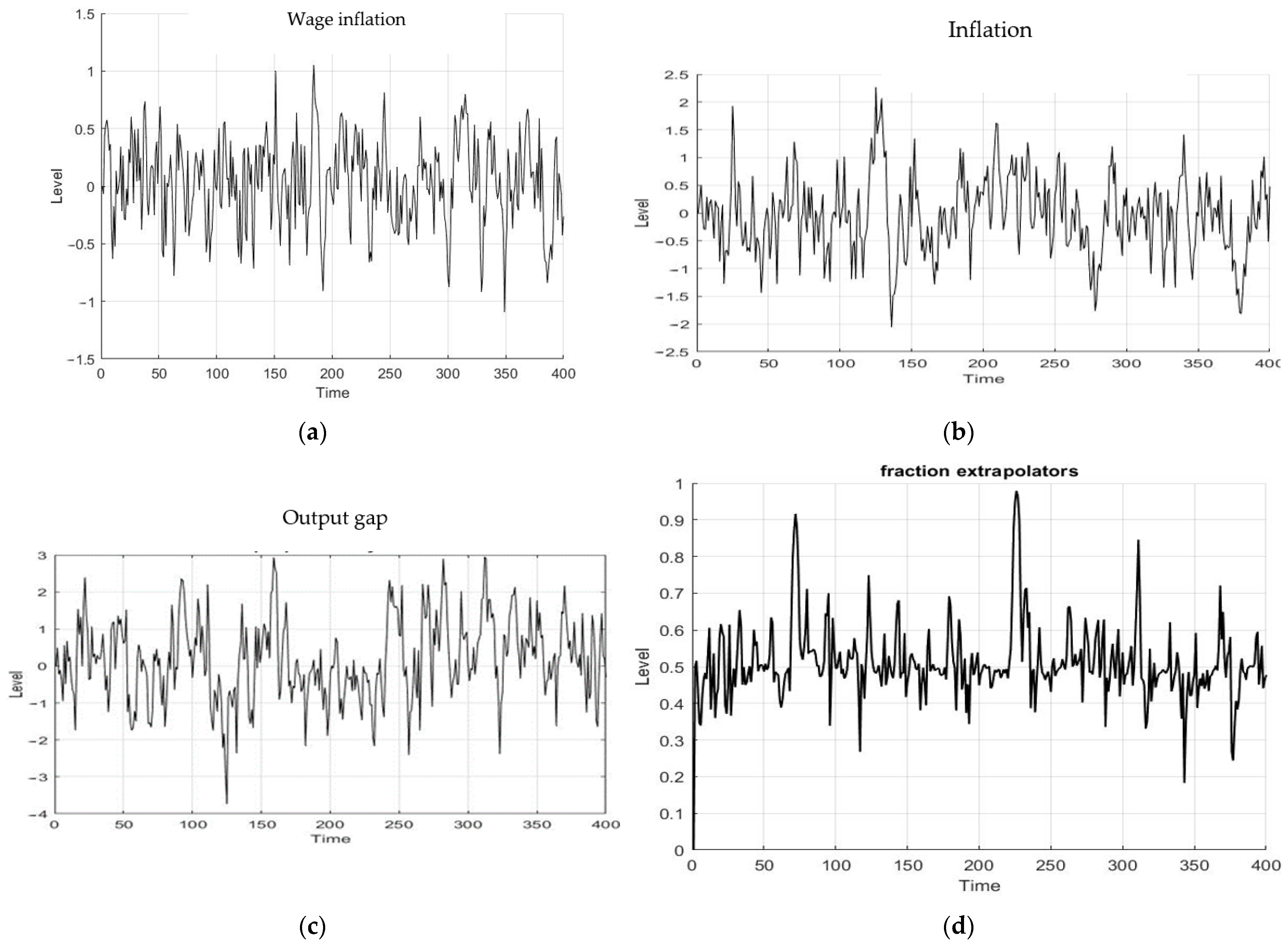
Figure 3 shows a strong cyclical movement of wage inflation, price inflation (hereinafter simply inflation) and the output gap in the studied behavioral model, the degree of cheerfulness of the agents of which corresponds to Figure 1a.

The source of these cyclical movements is the weighting of optimists and pessimists in the market. In fact, the model generates endogenous waves of optimism and pessimism. In some periods, pessimists predominate, leading to below-average output growth. These pessimistic periods are followed by optimistic ones, where optimistic forecasts prevail and the output growth rate is above average. These waves of optimism and pessimism are inherently unpredictable. Note that this figure shows the results of a simulation in which the five shocks present in Equations (6) and (14) are independent and equally distributed with a standard deviation of 0.5. Other implementations of shocks produce other cycles with the same overall characteristics.

These endogenously generated output cycles are made possible by a self-fulfilling mechanism, which can be described as follows. A series of random exogenous shocks creates the possibility that one of the two forecasting rules, say the optimistic one, provides a higher return, i.e., a lower mean-square forecast error. This attracts agents who used the pessimistic rule. The “contagion effect” leads to an increasing use of optimistic beliefs to predict, for example, an output gap, and this stimulates aggregate demand. Thus, optimistic moods are self-fulfilling. At some point, negative stochastic shocks are detrimental to optimistic forecasts. Pessimistic moods become attractive again and the economy is in recession. It can be shown that the periods of economic growth and recession coincide with the share of extrapolators and fundamentalists in the market. In Figure 2, under the output gap graph, there is a graph characterizing the change in the share of extrapolators in the market. It can be seen from this graph that the peaks in the output gap dynamics graph correspond to the peaks in the graph of changes in the share of extrapolators.

An analysis of the cycles shown in Figure 3 shows that the volatility of the output gap exceeds the volatility of price inflation and wage inflation. The volatility of the latter is less than the volatility of price inflation.

In macroeconomic models with rational expectations, only exogenous shocks matter to explain changes in output and inflation. There are important endogenously generated dynamics in the behavioral model that explain changes in output and inflation and influence the transmission of these exogenous shocks. Therefore, it is relevant to consider the transmission mechanism of action of some exogenous shocks in the model under study.

The behavioral model is non-linear. Therefore, in the post-shock period, it is necessary to take into account random perturbations, which are the same for a series with and without a shock. The simulations were repeated 1000 times with 1000 different implementations of random perturbations. Following this, the average impulse response was calculated along with the standard deviation. The shock sizes were equal to one standard deviation.

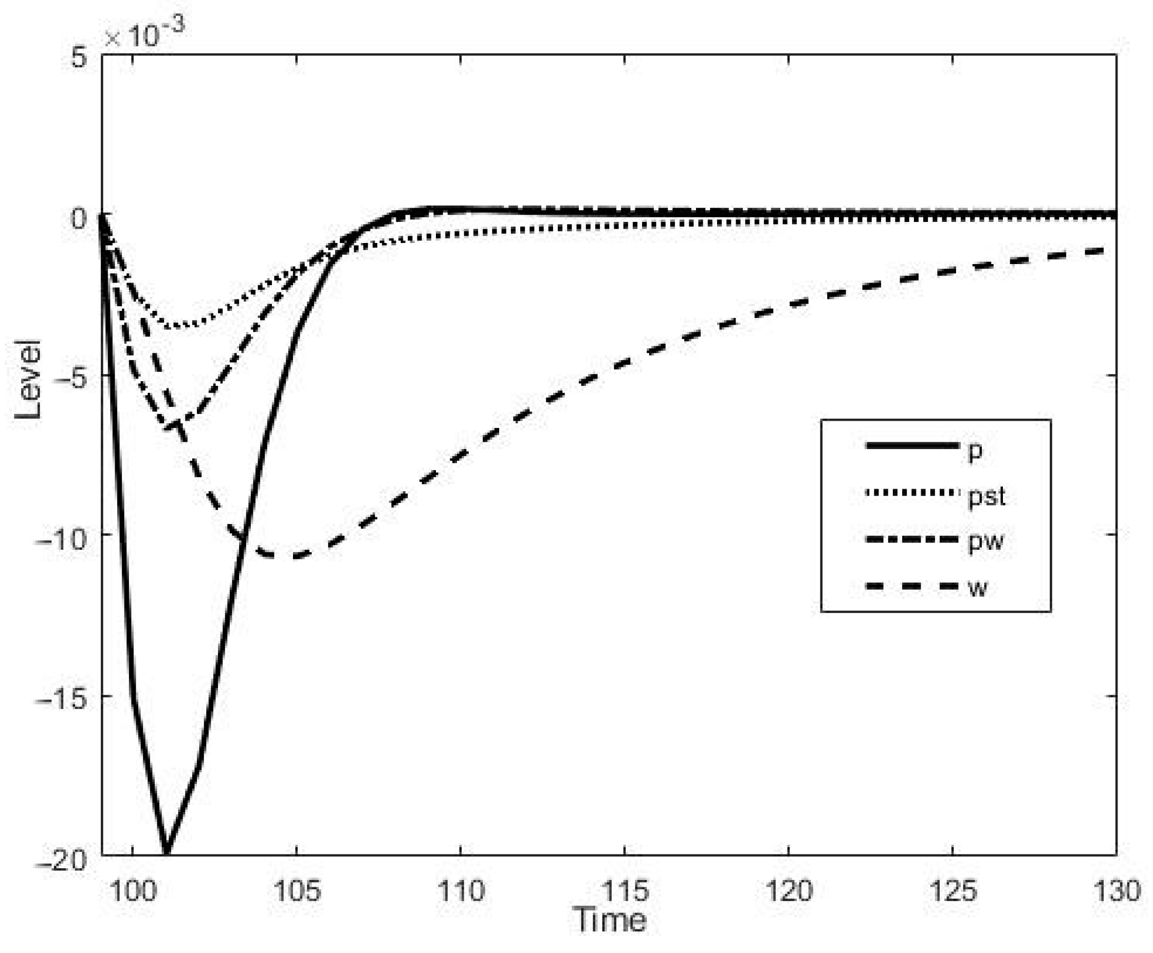
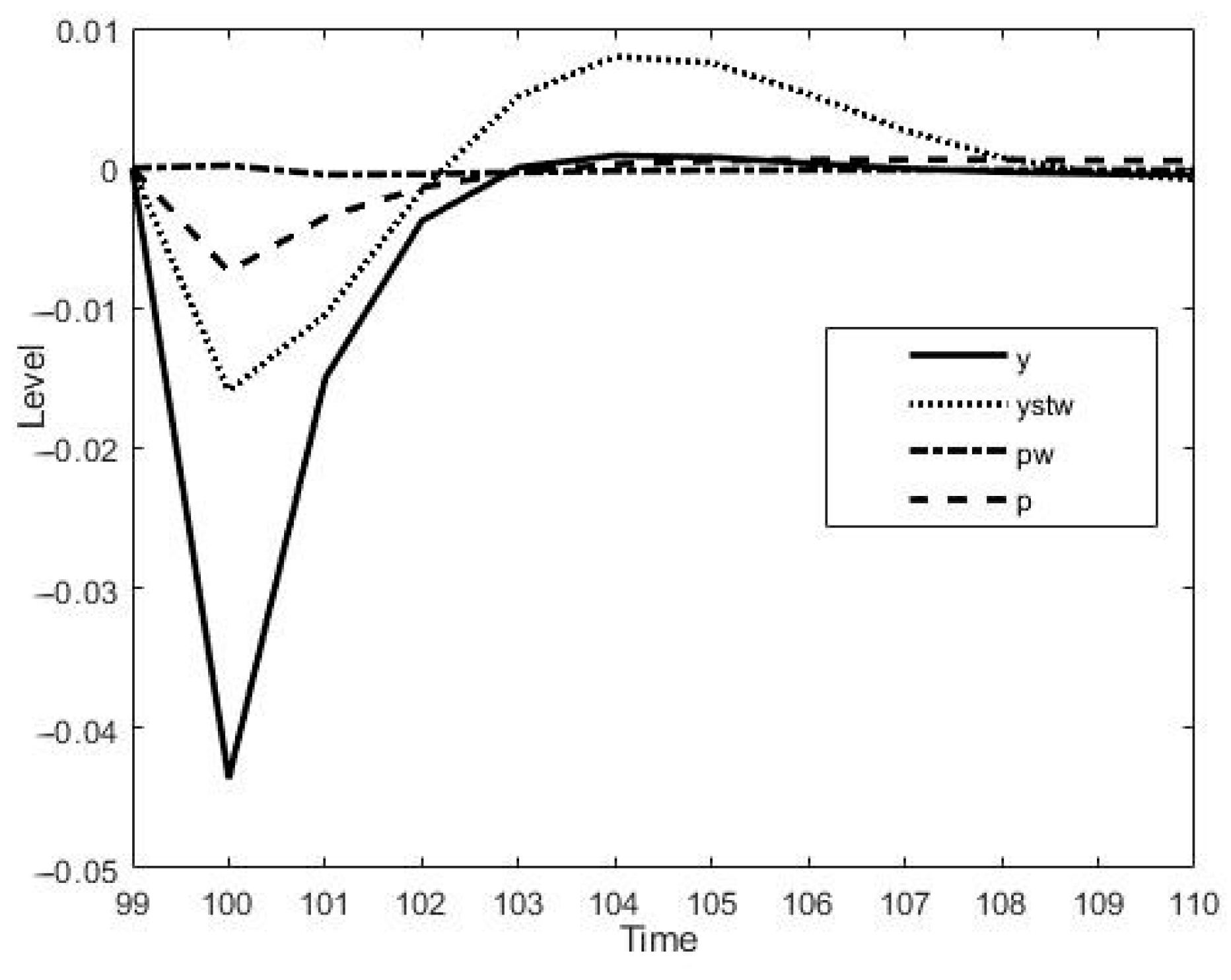
Figure 4 shows the effect of a temporary positive interest rate shock on the variables of the imperfect labor market model (wage inflation—pw, price inflation—pst, wage gap—w) and on the price inflation variable—p for the model with rigid prices and flexible wages.

The presence of both rigid wages and prices (the response shown by dashed lines) generates, unsurprisingly, a more muted wage inflation response compared to the price inflation of the underlying model with flexible wages and rigid prices (solid line) and compared to the gap response real wages of the first model (dotted lines). Finally, the most sluggish is the price inflation response (dotted lines) in the model with rigid wages and prices. As a result, the monetary authorities’ endogenous response to lower inflation implies higher interest rates. The sharper price inflation response in an economy with flexible wages (and rigid prices) is explained by the fact that the decline in activity as a response to a positive interest rate shock leads to a significant and permanent reduction in real wages, which increases the size of the fall in price inflation.

Figure 5 shows the impact of a temporary technology shock on the variables of the imperfect labor market model (wage inflation—pw, output gap ystw) and on the variables of the flexible wage and rigid price model (price inflation—p, output gap y).

From the analysis of the impulse responses of a positive technological shock, it follows that the wage inflation of a behavioral model with an imperfect labor market and rigid prices (dash-dotted line) practically does not change (and even slightly increases) as a result of a technological shock. Fairly sluggish response is also observed in the price inflation model with flexible wages and rigid prices (dashed line). The negative output gap response of the model with a perfect labor market and rigid prices is significant (solid line) and the output gap response of the model with an imperfect labor market and rigid prices is less profound (dotted line). The negative output gap is due to the fact that, as a result of a technological shock, the actual volume of output grows more slowly than the potential one for a given monetary policy. It is, however, true that in a model with an imperfect labor market, after several periods, the output gap becomes positive, in contrast to the base model.

When both prices and wages are rigid, monetary policy must strike a balance between achieving output and adjusting real wages due to productivity growth and, on the other hand, keeping wage and price inflation close to zero to avoid distortions associated with nominal volatility. Therefore, given the convexity of welfare losses in price and wage inflation, the monetary authorities and the government should increase real wages smoothly, combining negative price inflation and positive wage inflation, which is observed in Figure 5.

The resulting impulse responses are important. Based on their analysis, we can conclude that a more flexible economy is less prone to an economic cycle caused by abrupt waves of optimism and pessimism, different in nature to a more rigid economy. As mentioned above, the results obtained are original. The authors found confirmation of these results only in [28] for the New Keynesian model with rigid prices and flexible wages and in [44] for the neoclassical model. Thus, in the model under study, price flexibility is a determining factor in the self-organization of expectations and the self-development of this self-organization. The reason for this is as follows. Suppose there is a boom in economic activity: the output gap turns a positive. In a flexible economy, this increase in the output gap has a strong positive effect on inflation. Since the central bank places a high value on inflation in the Taylor rule, it reacts strongly by raising the interest rate. This tends to reduce the intensity of the boom. When the output gap widens in a rigid economy, this will have a weaker effect on inflation, forcing the central bank to raise interest rates less than in an elastic economy. The resulting boom in economic activity is stronger, which reinforces positive vitality, so that in a tight economy, the same initial shock in the output gap is more likely to cause an intense boom followed by a recession. Thus, a rigid economy will be more prone to booms and busts caused by a greater degree of animal spirits than a flexible economy. In other words, an economy with rigid prices and wages returns to a stationary state more slowly, having been brought out of it by exogenous shocks.

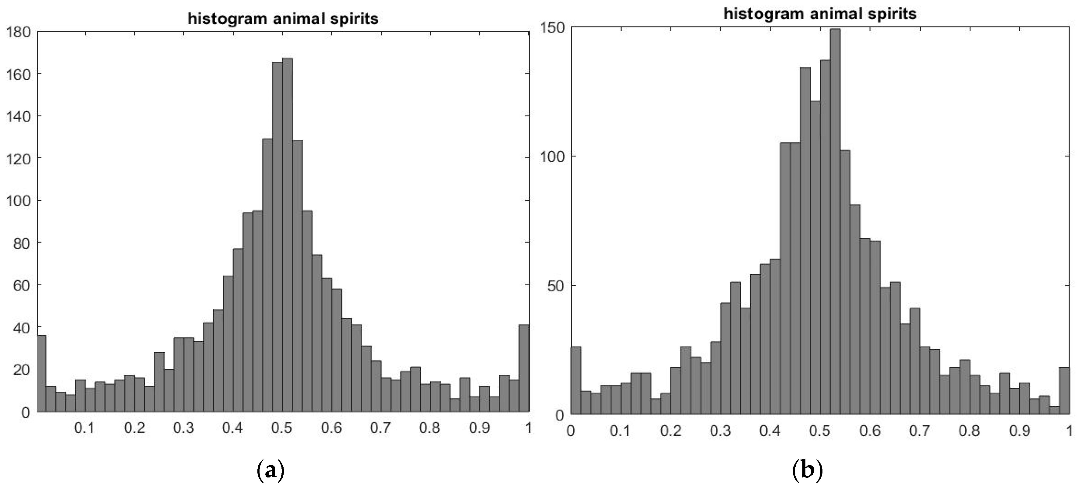
It is also very interesting to investigate what factors are the drivers of differences in the degree of vitality in the base model and in the model with rigid wages and prices (Figure 1). In other words, what factors are responsible for these differences when incorporating wage rigidity into the base model. Figure 6a shows a histogram of the frequency distribution of the degree of vitality for a model with an imperfect labor market when forecasting wage inflation using only the fundamentalist rule ${\tilde{E}}_t^{tar,w}{\pi }_{t+1}^w={\pi }^{w*}=0$ and with a coefficient of zero ${\varphi }_w$ in the Taylor rule for the interest rate. Figure 6b shows the histogram for the base model with fixed prices and flexible wages when predicting price inflation and the output gap using fundamental and extrapolation rules and non-zero coefficients ${\varphi }_{\pi },{\varphi }_y$ in the Taylor rule.

As follows from the figure, the histograms of the distribution of vital forces of both models are almost the same. From this we can conclude that the difference in the degree of vitality in the base model and in the model with fixed wages and prices is responsible for the complete trust of agents in the central bank in targeting wage inflation in the absence of the stabilization of this inflation by the bank.

Thus, the difference between the degree of optimism and pessimism in the baseline model and in the rigid wage and price model is due to the full confidence of agents in the central bank’s ability to target wage inflation. The central bank achieves this confidence in agents by responding more intensively to changes in inflation. This reduces the likelihood that the market will be dominated by extrapolators and, as a consequence, reduces the likelihood that agents will lose confidence in inflation targeting.

It should be noted that such a loss of confidence destabilizes both inflation and output. Thus, maintaining confidence in inflation targeting is an important source of macroeconomic stability in behavioral models.

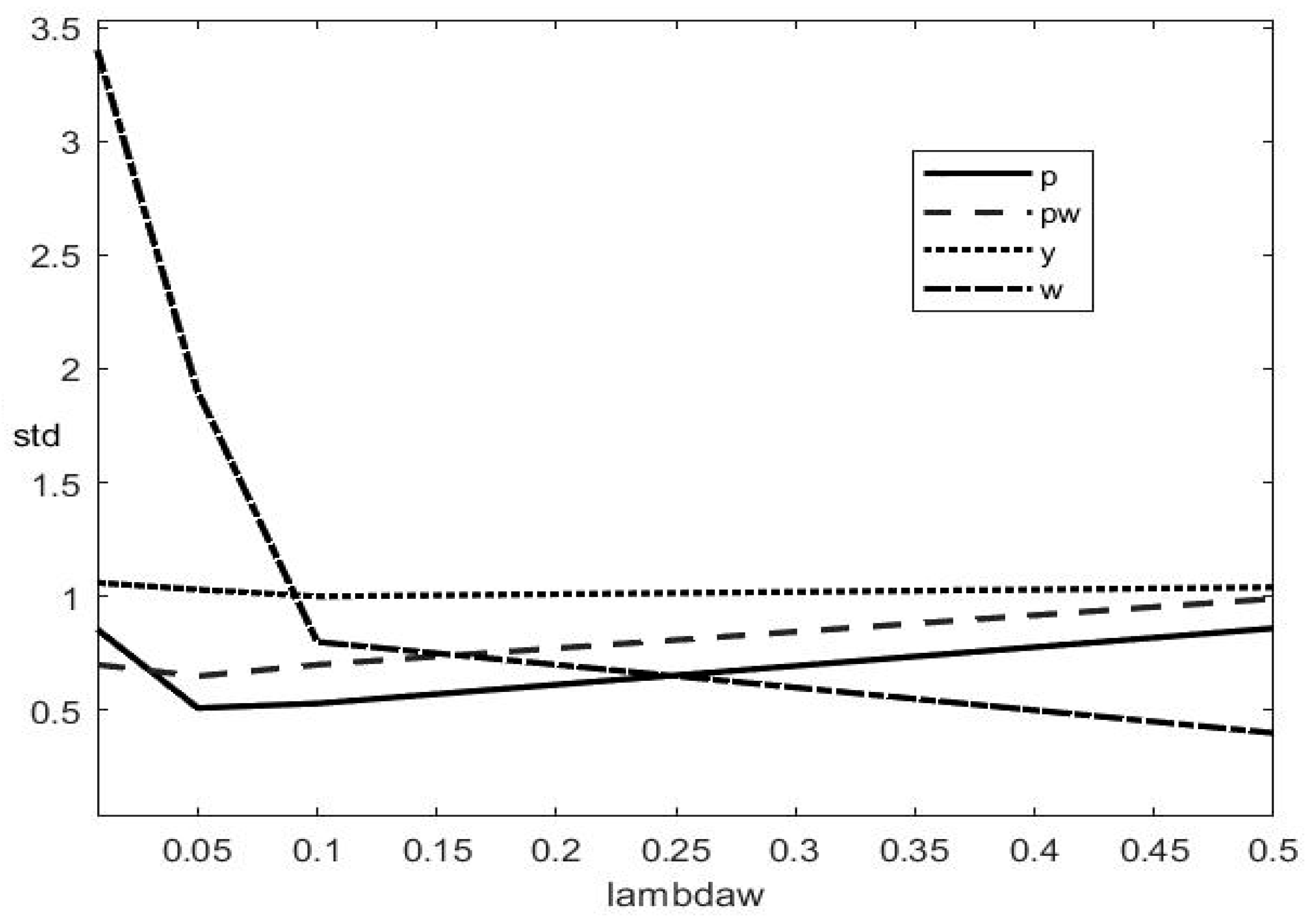
As it was mentioned above, the degree of wage rigidity depends on the parameter ${\lambda }_w$. The value of this parameter, corresponding to the values of the coefficients in Table 1, is 0.008. With an increase in the value of this parameter, the degree of wage rigidity decreases and its flexibility increases accordingly. Figure 7 plots the standard deviation (the standard deviation was calculated as the mean value obtained from 1000-fold simulations with 1000 different realizations of random exogenous shocks) of price inflation (p), wage inflation (pw), and output gap (y) against the degree of wage flexibility (lambdaw = ${\lambda }_w$) for a behavioral model with rigid wages and prices. The standard deviation is a measure of the volatility of the respective variables. At ${\lambda }_w=0.008$, the volatility of the output gap exceeds the volatility of price inflation and especially wage inflation. This exactly corresponds to the data in Figure 3. As follows from Figure 7, the volatility of the output gap remains almost unchanged with increasing wage flexibility. Wage inflation volatility increases with a small minimum around ${\lambda }_w=0.05$. The volatility of the wage gap decreases very sharply in the initial period and then gradually falls. The authors believe that this behavior is due to a decrease in real wages. An interesting dynamic is shown by the graph of price inflation with an initial sharp drop and a subsequent gradual increase in volatility. According to the authors, the sharp decline in the volatility of price inflation is due to a sharp drop in real wages. Wage inflation also reacts to the decline in real wages, but to a lesser extent.

The increase in the volatility of inflation in wages and prices with an increase in the parameter ${\lambda }_w$ is associated with the monetary policy of the central bank. As has been already noted, in the presence of two distortions—inflexible prices and inflexible wages—a single instrument of monetary policy cannot simultaneously compensate for both distortions. This can be shown that with an increase in the parameter ${\varphi }_{\pi }$ in the Taylor rule. Due to the limited publication format, these graphs are not shown. According to Equation (6), price inflation stabilizes (volatility becomes constant or decreases) in the absence of the stabilization of wage inflation and the output gap (its stabilization will be violated), the volatility of which will continue to increase, as in Figure 7.

The excess of the volatility of wage inflation as wage flexibility increases relative to the volatility of price inflation may suggest that the welfare cost of nominal rigidity is more related to wage rigidity than to price rigidity. The results shown in Figure 7 may be useful in stabilizing the considered variables.

4. Conclusions

In accordance with the purpose of the work, the changes and features of the economic agents’ behavior are analyzed when incorporating labor market imperfections (wage rigidity) into a new Keynesian behavioral model in comparison with a model with flexible wages and rigid prices (the basic model) with cognitive limitations of agents. At the same time, the forecasting of the output gap and the inflation of prices and wages occurs with the help of fundamentalist and extrapolation rules. The weight shares of agents applying these heuristics change endogenously generate endogenous waves of optimism and pessimism. An analysis of the impulse responses of interest rate and technology shocks suggests that a more flexible economy (an economy with flexible wages and rigid prices) is less prone to an abrupt economic cycle caused by waves of optimism and pessimism than a more rigid economy (an economy with an imperfect market labor). Thus, a rigid economy will be more prone to booms and busts caused by alternating optimism and pessimism than a flexible economy. The model with an imperfect labor market is characterized by an increased concentration of vital forces at the extreme values of 0 and 1, as well as in the middle of the distribution compared to the base model. This feature provides a key explanation for the non-normality of the dynamics of the evolution of variables. An original finding is that the entity responsible for the difference between the degree of optimism and pessimism in the baseline model and in the model with rigid wages and prices is the agents’ full confidence in the central bank in targeting wage inflation in the absence of the bank stabilization of this inflation. The dependence of the standard deviation of price inflation, wage inflation, and output gap on the degree of wage flexibility shows an increase in the volatility of all variables, except for the output gap, with a decrease in wage rigidity. These results may be useful in stabilizing the variables considered.

As it was already noted, the results obtained are original. Therefore, the authors cannot compare their results with others in terms of specific data for better integrative value of the study. The authors are aware that with other heuristic prediction rules, the results of the study may change. Therefore, the next step of the work is to collect and analyze data for a deeper and more comprehensive discussion of the findings in order to develop and deepen the research methodology.

References

1. Kydland, F.; Prescott, E. Time to build and aggregate fluctuations. Econometrica 1982, 50, 1345–1370. [Google Scholar] [CrossRef]
2. An, S.; Schorfheide, F. Bayesian analysis of DSGE models. Econom. Rev. 2007, 26, 113–172. [Google Scholar] [CrossRef]
3. Dubrovskaya, J.; Shults, D.; Kozonogova, E. Constructing a Region DSGE Model with Institutional Features of Territorial Development. Computation 2022, 10, 105. [Google Scholar] [CrossRef]
4. Muth, J.F. Rational expectations and the theory of price movements. Econometrica 1961, 29, 315–335. [Google Scholar] [CrossRef]
5. Sims, C. Solving rational expectations models. Comput. Econ. 2002, 20, 1–20. [Google Scholar] [CrossRef]
6. Sargent, T.; Wallace, N. Rational expectation and the theory of economic policy. J. Monet. Econ. 1976, 2, 169–183. [Google Scholar] [CrossRef]
7. Adam, K. Optimal monetary policy with imperfect common knowledge. J. Monet. Econ. 2007, 54, 267–301. [Google Scholar] [CrossRef]
8. Hommes, C. Behavioral and experimental macroeconomics and policy analysis: A complex systems approach. J. Econ. Lit. 2021, 1, 149–219. [Google Scholar] [CrossRef]
9. Massaro, D. Heterogeneous expectations in monetary DSGE models. J. Econ. Dyn. Control 2013, 37, 680–692. [Google Scholar] [CrossRef]
10. Andrade, P.; Bihan, H. Inattentive professional forecasters. J. Monet. Econ. 2013, 60, 967–982. [Google Scholar] [CrossRef] [Green Version]
11. Cornea-Madeira, A.; Hommes, C.; Massaro, D. Behavioral heterogeneity in U.S. inflation dynamics. J. Bus. Econ. Stat. 2019, 37, 288–300. [Google Scholar] [CrossRef]
12. Poledna, S.; Miess, M.G.; Hommes, C.; Rabitsch, K. Economic forecasting with an agent-based model. Eur. Econ. Rev. 2023, 151, 104306. [Google Scholar] [CrossRef]
13. Evans, G.W.; Hommes, C.; McGough, B.; Salle, I. Are long-horizon expectations (de-)stabilizing? Theory and experiments. J. Monet. Econ. 2022, 132, 44–63. [Google Scholar] [CrossRef]
14. Assenza, T.; Heemeijer, P.; Hommes, C.H.; Massaro, D. Managing self-organization of expectations through monetary policy: A macro experiment. J. Monet. Econ. 2021, 117, 171–186. [Google Scholar] [CrossRef]
15. Bao, T.; Hommes, C.; Pei, J. Expectation formation in finance and macroeconomics: A review of new experimental evidence. J. Behav. Exp. Financ. 2021, 32, 100591. [Google Scholar] [CrossRef]
16. Anufriev, M.; Hommes, C.; Makarewicz, T. Simple Forecasting Heuristics that Make us Smart: Evidence from Different Market Experiments. J. Eur. Econ. Assoc. 2019, 17, 1538–1584. [Google Scholar] [CrossRef]
17. Lennard, J. Sticky wages and the Great Depression: Evidence from the United Kingdom. Eur. Rev. Econ. Hist. 2022, heac014. [Google Scholar] [CrossRef]
18. Barattieri, A.; Basu, S.; Gottschalk, P. Some Evidence on the Importance of Sticky Wages. Am. Econ. J. Macroecon. 2014, 6, 70–101. [Google Scholar] [CrossRef]
19. Adrian, T.; Gaspar, V.; Vitek, F. A Medium-Scale DSGE Model for the Integrated Policy Framework. IMF Work. Pap. 2022, 2022, 99. [Google Scholar] [CrossRef]
20. Frenkel, J.; Froot, K. Using survey data to test standard propositions regarding exchange rate expectations. Am. Econ. Rev. 1987, 77, 133–153. [Google Scholar]
21. Frenkel, J.; Froot, K. Chartists, fundamentalists, and trading in the foreign exchange market. Am. Econ. Rev. 1988, 80, 181–185. [Google Scholar]
22. Carroll, C.D. Macroeconomic expectations of households and professional forecasters. Q. J. Econ. 2003, 118, 269–298. [Google Scholar] [CrossRef] [Green Version]
23. Branch, W.A. The theory heterogeneous expectations: Evidence from survey data on inflation expectations. Econ. J. 2004, 114, 592–621. [Google Scholar] [CrossRef]
24. Pfajfar, D.; Santoro, E. Heterogeneity, learning and information stickiness in inflation expectations. J. Econ. Behav. Organ. 2010, 75, 426–444. [Google Scholar] [CrossRef]
25. Hommes, C. The heterogeneous expectations hypothesis: Some evidence from the lab. J. Econ. Dyn. Control 2011, 35, 1–24. [Google Scholar] [CrossRef]
26. Driscoll, J.C.; Holden, S. Behavioral economics and macroeconomic models. J. Macroecon. 2014, 41, 133–147. [Google Scholar] [CrossRef]
27. De Grauwe, P. Animal spirits and monetary policy. Econ. Theory 2011, 47, 423–457. [Google Scholar] [CrossRef]
28. De Grauwe, P. Booms and busts in economic activity: A behavioral explanation. J. Econ. Behav. Organ. 2012, 83, 484–501. [Google Scholar] [CrossRef]
29. De Grauwe, P. Lectures on Behavioral Macroeconomics; Princeton University Press: Princeton, NJ, USA, 2012. [Google Scholar]
30. Galí, J. Monetary Policy, Inflation and the Business Cycle. An Introduction to the New Keynesian Framework and Its Applications, 2nd ed.; Princeton University Press: Princeton, NJ, USA, 2015. [Google Scholar]
31. Erceg, C.; Dale, W.; Levin, A. Optimal monetary policy with staggered wage and price contracts. J. Monet. Econ. 2000, 46, 281–313. [Google Scholar] [CrossRef]
32. Mankiw, N.; Reis, R.; Wolfers, J. Disagreement About Inflation Expectations, NBER. Macroecon. Annu. 2004, 18, 209–270. [Google Scholar] [CrossRef]
33. Branch, W.; McGough, B. A New Keynesian model with heterogeneous expectations. J. Econ. Dyn. Control 2009, 33, 1036–1051. [Google Scholar] [CrossRef]
34. Brock, W.; Hommes, C. A rational route to randomness. Econometrica 1997, 65, 1059–1095. [Google Scholar] [CrossRef]
35. Sargent, T. Bounded Rationality in Macroeconomic; Oxford University Press: Oxford, UK, 1993. [Google Scholar]
36. Evans, G.; Honkapohja, S. Learning and Expectations in Macroeconomics; Princeton University Press: Princeton, NJ, USA, 2001; 421p. [Google Scholar]
37. Gaspar, V.; Smets, F.; Vestin, D. Adaptive Learning, Persistence and Optimal Monetary Policy. J. Eur. Econ. Assoc. 2006, 4, 376–385. [Google Scholar] [CrossRef]
38. Orphanides, A.; Williams, J. Robust Monetary Policy with Imperfect Information; Board of Governors of the Federal Reserve System: Washington, DC, USA, 2004. [Google Scholar]
39. Milani, F. Learning and Time-Varying Macroeconomic Volatility. J. Econ. Dyn. Control 2014, 47, 94–114. [Google Scholar] [CrossRef]
40. Calvo, A. Staggered Prices in a Utility-Maximizing Framework. J. Monet. Econ. 1983, 12, 383–398. [Google Scholar] [CrossRef]
41. Christiano, L.; Eichenbaum, M.; Evans, C. Nominal Rigidities and the Dynamic Effects of a Shock to Monetary Policy. J. Political Econ. 2005, 113, 1–45. [Google Scholar] [CrossRef]
42. Branch, W.; Evans, G. A simple recursive forecasting model. Econ. Lett. 2006, 91, 158–166. [Google Scholar] [CrossRef]
43. Brazier, J.; Tumur, I.; Holmes, M.; Ferriter, M.; Parry, G. Psychological therapies including dialectical behaviour therapy for borderline personality disorder: A systematic review and preliminary economic evaluation. Health Technol. Assess. 2006, 10, 1–117. [Google Scholar] [CrossRef] [PubMed] [Green Version]
44. Serkov, L.A. Self-organization of expectations as a factor of self-development of economic systems. J. New Econ. 2014, 53, 100–106. [Google Scholar]
Figure 1. The histogram of the frequency distribution of the degree of optimism and pessimism: (a) for the model under study with an imperfect labor market and rigid prices; (b) for the basic model with fixed prices and flexible wages.
Mathematics 11 00796 g001
Figure 2. Histogram of the frequency distribution of the degree of animal spirits for the model under study with an imperfect labor market at a value λ w = 0.1 .
Mathematics 11 00796 g002
Figure 3. Schedules of cyclical movement: (a) wage inflation; (b) price inflation; (c) output gap; (d) shares of extrapolators in the studied behavioral model.
Mathematics 11 00796 g003
Figure 4. The effect of a positive interest rate shock on the variables of the behavioral model with an imperfect labor market (pw is wage inflation, pst is price inflation, w is the wage gap) and on the price inflation variable p of the model with fixed prices and flexible wages. The shock value is equal to one standard deviation.
Mathematics 11 00796 g004
Figure 5. The impact of a positive technology shock on the variables of the behavioral model with an imperfect labor market (pw is wage inflation; ystw is the output gap) and on the variables of the model with flexible wages and rigid prices (p is price inflation, y is the output gap). The shock value is equal to one standard deviation.
Mathematics 11 00796 g005
Figure 6. (a) a histogram of the frequency distribution of the degree of vitality for a model with an imperfect labor market when forecasting wage inflation only using the fundamentalist rule (24) and with a zero coefficient ϕ w in the Taylor rule for the interest rate; (b) Histogram for the base model with fixed prices and flexible wages for price inflation and output gap forecasting using two rules and non-zero coefficients ϕ π , ϕ y in the Taylor rule. The coefficients for both models correspond to those of Table 2.
Mathematics 11 00796 g006
Figure 7. Standard deviation (std) of price inflation (p), wage inflation (pw), output gap (y), and real wage gap (w) as a function of wage flexibility (lambdaw). Model with rigid wages and prices with monetary policy parameters given in Table 2 ( ϕ π = 1.5 ,   ϕ w = ϕ y = 0.5 ) .
Mathematics 11 00796 g007