Time-Optimal Problem in the Roto-Translation Group with Admissible Control in a Circular Sector

Abstract

We study a time-optimal problem in the roto-translation group with admissible control in a circular sector. The problem reveals the trajectories of a car model that can move forward on a plane and turn with a given minimum turning radius. Our work generalizes the sub-Riemannian problem by adding a restriction on the velocity vector to lie in a circular sector. The sub-Riemannian problem is given by a special case when the sector is the full disc. The trajectories of the system are applicable in image processing to detect salient lines. We study the local and global controllability of the system and the existence of a solution for given arbitrary boundary conditions. In a general case of the sector opening angle, the system is globally but not small-time locally controllable. We show that when the angle is obtuse, a solution exists for any boundary conditions, and when the angle is reflex, a solution does not exist for some boundary conditions. We apply the Pontryagin maximum principle and derive a Hamiltonian system for extremals. Analyzing a phase portrait of the Hamiltonian system, we introduce the rectified coordinates and obtain an explicit expression for the extremals in Jacobi elliptic functions. We show that abnormal extremals are of circular type, and they correspond to motions of a car along circular arcs of minimal possible radius. The normal extremals in a general case are given by concatenation of segments of sub-Riemannian geodesics in ${SE}_2$ and arcs of circular extremals. We show that, in a general case, the vertical (momentum) part of the extremals is periodic. We partially study the optimality of the extremals and provide estimates for the cut time in terms of the period of the vertical part.

1. Introduction

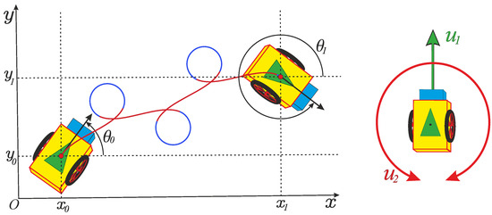
Consider a car model that can move forward on a plane and turn with a given minimum turning radius (see Figure 1). The car has two wheels, equidistant from the axle of the wheelset. Both wheels have independent drives that can rotate so that the corresponding rolling of the wheels occurs without slipping. The configuration of the system is described by the triple $q=(x,y,\theta )={\mathbb{R}}^2\times S^1$, where $(x,y)\in {\mathbb{R}}^2$ is the central point, and $\theta \in S^1$ is the orientation angle of the car. In such a way, the configuration space forms the Lie group of roto-translations ${SE}_2\simeq {\mathbb{R}}^2\times S^1.$

Figure 1. A model of a car that can move forward and turn within a given minimal radius. The control $u_1$ is responsible for moving forward and $u_2$ for the turn.

The car has two controls: the tangential velocity $u_1$ and the angular velocity $u_2$. Consider the configuration $Id=(0,0,0)$, when the car is located at the origin and oriented along the positive direction of $Ox$. An infinitesimal translation is generated by the vector ${\partial }_x$ and rotation by the vector ${\partial }_{\theta }$. They are possible motions controlled by $u_1$ and $u_2$. The remaining direction ${\partial }_y$ is forbidden since the immediate motion of the car in a direction perpendicular to its wheels is not possible. Thus, the dynamics of the car at the origin is given by $\dot{x}=u_1$, $\dot{y}=0$, and $\dot{\theta }=u_2$.

The origin Id is the unit element of the group ${SE}_2$ (see Section 2). Any element $q\in {SE}_2$ is generated by the left translation $L_q$ Id. The dynamics at an arbitrary configuration q are

$$\dot{q}=u_1{X}_1\left(q\right)+u_2{X}_2\left(q\right),$$

(1)

where $X_i$ represents left-invariant vector fields (see Section 2).

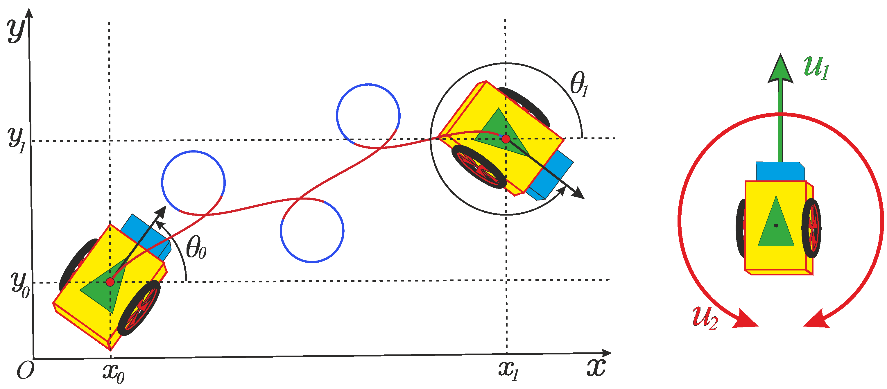
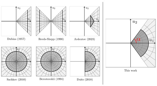
Various sets of admissible controls $U\ni (u_1,u_2)$ lead to different models (see Figure 2). The time-optimal problem for

Figure 2. Set of admissible controls for various models of a car on a plane: Dubins car [1]; Reeds–Shepp car [2]; Ardentov model [3] (generalized Dubins car); Sachkov model [4] (sub-Riemannian problem); Berestovskii model [5]; Duits model [6]; our model with control in a sector.

• $u_1=1$, $|u_2|\le \kappa$, $\kappa >0$ leads to Dubins car [1];
• $|u_1|=1$, $|u_2|\le \kappa$, $\kappa >0$ leads to Reeds–Shepp car [2];
• $u_1\ge 1$, $u_1+\left|u_2\right|\le \kappa <1$ leads to a generalized Dubins car, studied by Ardentov [3];
• $u_1^2+u_2^2\le 1$ leads to the model whose solutions are sub-Riemannian length minimals, studied by Sachkov [4];
• $u_1^2+u_2^2\le 1$, $u_1\ne 0$ leads to the model studied by Berestovskii [5];
• $u_1\ge 0$, $u_1^2+u_2^2\le 1$ leads to the model of a car moving forward and turning in place, proposed by Duits [6];
• $u_1=rcos\varphi$, $u_2=rsin\varphi$, $0\le r\le 1$, $\left|\varphi \right|\le \alpha$ leads to the general model of a car with control in a circular sector, which is studied in this paper.

In 1957, Dubins described [1] the problem of finding the shortest path for a car in plane moving with no reverse gear from an initial configuration (position and direction) to a final configuration penalizing the curvature of its trajectory in the plane. Later in 1990, Reeds and Shepp studied [2] the same problem, but for a car that has reverse gear. Both papers are devoted to a description of the general shape of the optimal paths, without providing explicit solutions for given boundary conditions. It was shown that the optimal trajectories of Dubins and Reeds–Shepp cars are given by concatenation of arcs of a circle of minimum possible radius (circular trajectories) and segments of a straight line (straight trajectories). In a recent study [3], Ardentov refines the Dubins model by considering the bounded angular speed of two wheels, which results in maximal tangential speed when the car is moving straight. For the refined model, extremal trajectories have been found. They are also given by concatenation of circular and straight trajectories. Note that such trajectories have bounded curvature: the upper bound is given by reciprocal to the minimal turning radius.

In 2011, Sachkov [4] obtained optimal synthesis in a sub-Riemannian problem in ${SE}_2$. This problem can be seen as the shortest path problem for a car that can move forward/backward and turn in place. In such a model, the curvature of trajectories is unbounded, and it was shown that optimal trajectories may contain cusp points, the points where the direction of motions is switching to the opposite one. Berestovskii [5] studied segments of the trajectories that contain no cusps and can be parameterized by the length of the planar projection.

In 2018, Duits and coauthors [6] studied a modification of the sub-Riemannian problem obtained by the restriction of the reverse gear. In the Duits model, the car can move forward and rotate in place, but it cannot move backward. Motivation came from image analysis applications, where the trajectories of the car are used to detect salient lines in images. An exact expression for the extremals was obtained in [7]. The original idea of the Duits model was to reduce the number of undesirable cusp points by suppressing the backward motions. However, it turned out that the cusp points are replaced by turning points (the points of in-place rotation on $\pi$ radians), and the projection of extremal trajectories of the Duits car to the image plane coincide with the projection of sub-Riemannian geodesics in ${SE}_2$. This observation shows that in order to entirely solve the “cusp problem”, the model needs further adaptation. In the present paper, we propose a model of a car that can move forward, stay in place, and turn with a given minimal turning radius. Trajectories of this system a priori cannot have cusp points in the planar projection.

The problem of transferring the car between the given initial and final configurations is known in robotics as a motion planning problem. There are different approaches to tackle this problem [8]. Introducing a cost function for the system leads to an optimal control problem. Such optimal control problems are tackled by various numerical methods, see, e.g., [9]. However, exact solutions (optimal synthesis) are known only for a few of the simplest models in robotics [4,10]. In the present paper, we obtain explicit expressions for extremals in a more complicated model with control in a circular sector.

System (1) arises in the modeling of the human visual system. An important discovery of the neurophysiology of vision was made by Hubel and Wiesel in 1959 [11], who showed that in the striate cortex of a cat, there exist groups of neurons sensitive to positions and directions (orientations). In the first stage of processing, the image is lifted by the brain to the extended space of positions and directions. In [12], a sub-Riemannian structure on the Heisenberg group was proposed for contour perception and completion. The model was refined in [13] by taking into account the global nature of the orientation angle. The roto-translation group ${SE}_2$ endowed with a sub-Riemannian metric has been proposed to model the functional architecture of the primary visual cortex. This model is known as the Petiot–Citti–Sarti model, where sub-Riemannian geodesics (extremal trajectories) are used for the completion of occluded contours. The usage of sub-Riemannian geodesics for modeling the association field in the psychophysiology of vision was studied in [14]. It was shown that good candidates for the association field lines are given by sub-Riemannian geodesics with cuspless planar projection. Application of sub-Riemannian geodesics for modeling illusory contours in geometrical optical illusions has been studied in [15,16].

The principles of biological visual systems are actively used in computer vision. Based on these principles, effective image processing methods are created, e.g., image reconstruction [17] and detection of salient lines in images [18,19]. In [18], optimal trajectories of a System (1) are used to detect salient lines in images. The motivation for our study is to solve the problem of cusp points that appear in the salient line detection method [18], which is based on tracking via sub-Riemannian geodesics. At such points, the car reverses its direction of motion, and a detected salient line has an undesirable cusp point. In our model with control in a circular sector with an acute opening angle, the cusp points are impossible.

Our work generalizes the sub-Riemannian problem [4] by adding a restriction on the velocity vector to lie in a circular sector. The sub-Riemannian problem is given by a special case when the sector is the full disc. In addition to its importance for applications, the problem under study is of independent interest in geometric control theory [20] as a model example of an optimal control problem in which zero control lies on the boundary of the set of control parameters.

The problem can be seen as a rolling geodesic problem [21,22], where a disc is rolling on a plane. We explicitly derive the geodesics and analyze their optimality.

In the present paper, we study the time-optimal problem for System (1) with control in a circular sector. We generalize the results [7], where we studied the special case of admissible controls in a half-disc. The present paper is an extended version of the preliminary work [23], where we studied the case of the sector opening angle less than $\pi$ and parameterized the extremal trajectories by the length of their planar projection (s–parametrization). Now we study the general case of the sector opening angle and derive the explicit formulas for the time-parameterized extremals (t–parametrization), which is natural for time-optimal problems. We also provide an analysis of their optimality.

The present paper is organized as follows. In Section 2, we give preliminary materials on the Lie group ${SE}_2$. In Section 3, we formulate an optimal control problem under consideration. In Section 4, we study local and global controllability (see Definitions 1–3) of the system and the existence of a solution for given arbitrary boundary conditions. In Section 5, we apply a necessary optimality condition, the Pontryagin maximum principle (PMP), and describe a phase portrait of the Hamiltonian system of PMP. In Section 6, we integrate the Hamiltonian system and obtain an explicit expression for the extremals. In Section 7, we partially study the optimality of the extremals and provide estimates for the cut time.

2. Preliminaries

The roto-translation group ${SE}_2$ is the group of proper motions of the Euclidean plane. Any such motion $q=(x,y,\theta )\in {SE}_2$ consists of a rotation around a given point on angle $\theta \in S^1=\mathbb{R}/2\pi \mathbb{Z}$ and a parallel translation on a vector $(x,y)\in {\mathbb{R}}^2$.

The composition of two motions results in the product of two elements $q^{\prime },q\in {SE}_2$:

$$q^{\prime }·q=(xcos{\theta }^{\prime }-ysin{\theta }^{\prime }+x^{\prime },xsin{\theta }^{\prime }+ycos{\theta }^{\prime }+y^{\prime },\theta +{\theta }^{\prime }).$$

The identical transformation of the plane is the unit element $Id=(0,0,0)\in {SE}_2$.

For any $q\in {SE}_2$, there exists $q^{-1}\in {SE}_2$ such that $q^{-1}·q=q·q^{-1}=Id$ given by

$$q^{-1}=(-xcos\theta -ysin\theta ,xsin\theta -ycos\theta ,-\theta ).$$

Note that the group operation is not commutative. The left translation is defined as

$$L_{q^{\prime }}q=q^{\prime }·q.$$

The tangent space $T_{Id}{SE}_2=span({\partial }_x,{\partial }_y,{\partial }_{\theta })$ with the Lie bracket operation

$$[{\partial }_x,{\partial }_y]=0,[{\partial }_x,{\partial }_{\theta }]=-{\partial }_y,[{\partial }_y,{\partial }_{\theta }]={\partial }_x$$

forms the Lie algebra ${\mathfrak{se}}_2$. It is isomorphic to the Lie algebra of the left-invariant vector field $span(X_1,X_2,X_3)$, where the vector fields $X_i$ are obtained via push-forward

$$\begin{array}{ccc}& & X_1\left(q\right)=L_{q\ast }{\partial }_x=cos\theta {\partial }_x+sin\theta {\partial }_y,\hfill \\ & & X_2\left(q\right)=L_{q\ast }{\partial }_{\theta }={\partial }_{\theta },\hfill \\ & & X_3\left(q\right)=L_{q\ast }(-{\partial }_y)=sin\theta {\partial }_x-cos\theta {\partial }_y.\hfill \end{array}$$

3. Statement of the Problem

For a given angle $\alpha \in [0,\pi ]$, consider the following control system:

$$\left\{\begin{array}{c}\dot{x}=u_{1}cos\theta ,\hfill \\ \dot{y}=u_{1}sin\theta ,\hfill \\ \dot{\theta }=u_2,\hfill \end{array}\right.\begin{array}{c}(x,y,\theta )=q\in {SE}_2,\hfill \\ (u_1,u_2)\in U,\hfill \\ U=\left\{\right(rcos\varphi ,rsin\varphi \left)\right|0\le r\le 1,\left|\varphi \right|\le \alpha \}.\hfill \end{array}$$

(2)

For given boundary conditions $q_0$, $q_1\in {SE}_2$, we aim to find the controls $u_1\left(t\right)$, $u_2\left(t\right)\in L^{\infty }([0,T],\mathbb{R})$ such that the corresponding trajectory $q:[0,T]\to {SE}_2$ transfers the system from the initial $q_0$ to the final configuration $q_1$ in minimal time:

$$q\left(0\right)=q_0,q\left(T\right)=q_1,T={\int }_0^T\mathrm{d}t\to min.$$

(3)

Remark 1. 

The problem is invariant under the left action of ${SE}_2$ since the vector fields $X_1$ and $X_2$ are left-invariant. Due to this property without loss of generality, we set $q\left(0\right)=Id$.

4. Existence of the Solution

4.1. Controllability and Existence of Optimal Controls

In this section, we study the existence of the solution in Problem (2), (3). First, we give some necessary definitions.

Denote by $\mathcal{A}$ the attainable set [20] of System (2) from Id for any non-negative time.

Definition 1. 

System (2) is called globally controllable if $\mathcal{A}={SE}_2$.

In other words, a control system is globally controllable if any two points of its configuration space can be connected by an admissible trajectory.

Let $t\ge 0$. Denote by ${\mathcal{A}}_{\le t}$ the attainable set of System (2) from $Id\in {SE}_2$ for time $\le t$. Denote by $int{\mathcal{A}}_{\le t}$ the interior of the set ${\mathcal{A}}_{\le t}$.

Definition 2. 

System (2) is called small-time locally controllable at Id if for all $t>0$, there holds the inclusion $int{\mathcal{A}}_{\le t}\ni Id.$

Definition 3. 

System (2) is called locally controllable for time $t>0$ at Id if $int{\mathcal{A}}_{\le t}\ni Id.$

Next, we provide an analysis of global and small-time local controllability of System (2) and study the existence of optimal control. We show that there are four different possible cases depending on the domain of angle $\alpha$. The result is gathered in Theorem 1.

Theorem 1. 

Consider Problem (2), (3) with $q_0=Id$. The following statements hold:

1.

For $\alpha =0$, the system is not globally controllable. The attainable set is $\mathcal{A}=\left\{\right(x,0,0\left)\right|x\ge 0\}$. For any $q_1\in \mathcal{A}$, there exists a unique optimal trajectory;

2.

For $\alpha \in (0,\frac{\pi }{2}]$, the system is globally controllable, but not small-time locally controllable. For any $q_1\in {SE}_2$, there exists an optimal trajectory;

3.

For $\alpha \in (\frac{\pi }{2},\pi )$, the system is globally controllable and small-time locally controllable. An optimal trajectory does not exist for some boundary conditions;

4.

For $\alpha =\pi$, the system is globally and small-time locally controllable. For any $q_1\in {SE}_2$, there exists an optimal trajectory.

Proof. 

First, we show that the system is not globally controllable if $\alpha =0$. Indeed, when $\alpha =0$, System (2) is reduced to $\dot{q}=u_1{X}_1\left(q\right)$, $u_1\in [0,1]$, $q\left(0\right)=Id$, and the attainable set ${\mathcal{A}}_{\le t}$ is a segment of the trajectory $e^{\tau X_1}(Id)=(\tau ,0,0)$, $0\le \tau \le t$. Consequently, the attainable set for any non-negative time is a ray $\mathcal{A}=\left\{\right(x,0,0\left)\right|x\ge 0\}$. The optimal control is given by $u_1\equiv 1$, and there exists a unique optimal trajectory, a segment of a straight line, which transfers the system from Id to any element $q_1\in \mathcal{A}$.

Next, we provide three different proofs of global controllability for $\alpha \ne 0$. The global controllability of System (2) for $\alpha \ne 0$ follows from the global controllability of Dubins car (see [1]). Indeed, the sets of admissible trajectories of the two systems are the same, since the convex cones of the sets of admissible controls in these problems coincide with one another. Thus, the controllability of the Dubins car is equivalent to the controllability of our problem. The second proof follows from the general statement in [24]. According to [24], a left-invariant system is globally controllable on ${SE}_2$ if and only if the system is full-rank (bracket generating), i.e., the Lie algebra at every point forms the full tangent space. We have $Lie(cos\alpha X_1+sin\alpha X_2,cos\alpha X_1-sin\alpha X_2)=span(X_1,X_2,X_3)$, thus System (2) is globally controllable. The third proof of controllability is given in [23]. It relies on the Lie saturation method (see [20]), which is standard in geometric control theory.

Now we study the case $\alpha \in (0,\frac{\pi }{2}]$. For any $u\in U$, we have $u_1\ge 0$. Thus,

$$x\left(t\right)={\int }_0^t{u}_1\left(\tau \right)cos\theta \left(\tau \right)\mathrm{d}\tau \ge 0\mathrm{for}\mathrm{small}t>0.$$

Consequently, System (2) is not small-time locally controllable for $\alpha \in (0,\frac{\pi }{2}]$. Further, in Theorem 2, we give a precise time estimate for local controllability in this case. The existence of an optimal trajectory that transfers the system for $\alpha \in (0,\frac{\pi }{2}]$ from Id to any $q_1\in {SE}_2$ is guaranteed by the Filippov theorem [20]. Indeed, all the conditions of the Filippov theorem hold due to the compactness and convexity of U and the global controllability of the system.

Next, we analyze the case $\alpha \in (\frac{\pi }{2},\pi )$. First, we show that the system is small-time locally controllable. To this end, we consider a convex closure $V=co\left(U\right)$ of the set U and the corresponding relaxed control system (2) with the set of admissible controls $V\ni (u_1,u_2)$. Denote by ${\mathcal{B}}_{\le t}$ the attainable set of the relaxed system by time $\le t$. Since $0\in intV$ and the relaxed system is full-rank, it is small-time locally controllable, i.e., for all $t>0$, we have $int{\mathcal{B}}_{\le t}\ni Id$. By Thm. 8.2 of [20], the attainable sets of the original and the relaxed systems are related by ${\mathcal{B}}_{\le t}\subset \overline{{\mathcal{A}}_{\le t}}$, where $\overline{S}$ is the closure of a set S. Thus, $int\overline{{\mathcal{A}}_{\le t}}\ni Id$. Since the original system is full-rank, we have $int{\mathcal{A}}_{\le t}\ni Id$, and hence we prove that the system is small-time locally controllable.

In the case $\alpha \in (\frac{\pi }{2},\pi )$, the set U is not convex. Now we show that there exists a boundary condition $q_1$ for which an optimal trajectory does not exist. Consider $q_1=(cos\alpha ,0,0)$. We show that it satisfies the following conditions:

(a)

$inf\{t_1>0|\mathrm{there}\mathrm{exists}\mathrm{a}\mathrm{trajectory}q(·),\mathrm{s}.\mathrm{t}.q\left(0\right)=Id,q\left(t_1\right)=q_1\}\le 1$;

(b)

A trajectory $q(·)$, s.t. $q\left(0\right)=Id,q\left(1\right)=q_1$ does not exist.

It is obvious that Conditions (a) and (b) imply the nonexistence of optimal trajectory connecting Id and $q_1$. Let us prove Item (a). Let $n\in \mathbb{N}$. Consider the following control:

$$\begin{array}{ccc}& & t\in \left[\frac{i}{n},\frac{2i+1}{2n}\right)\Rightarrow u_1\left(t\right)=cos\alpha ,u_2\left(t\right)=sin\alpha ,\hfill \end{array}$$

(4)

$$\begin{array}{ccc}& & t\in \left[\frac{2i+1}{2n},\frac{i+1}{n}\right]\Rightarrow u_1\left(t\right)=cos\alpha ,u_2\left(t\right)=-sin\alpha .\hfill \end{array}$$

(5)

For $u_1=cos\alpha$, $u_2=\pm sin\alpha$, the corresponding trajectory satisfies the following ODE:

$$\dot{x}=cos\alpha cos\theta ,\dot{y}=cos\alpha sin\theta ,\dot{\theta }=\pm sin\alpha ,(x,y,\theta )\left(0\right)=(x_0,y_0,{\theta }_0),$$

and is given by

$$\begin{array}{ccc}& & x\left(t\right)=x_0\pm cot\alpha \left(sin({\theta }_0\pm tsin\alpha )-sin{\theta }_0\right),\hfill \\ & & y\left(t\right)=y_0\mp \left(cos({\theta }_0\pm tsin\alpha )-cos{\theta }_0\right),\hfill \\ & & \theta \left(t\right)={\theta }_0\pm tsin\alpha .\hfill \end{array}$$

Thus, the trajectory $(x,y,\theta )\left(t\right)$ with Controls (4) and (5) departing from Id has an end point

$$\begin{array}{ccc}& & x\left(1\right)=x^n=2ncot\alpha sin\left(\frac{sin\alpha }{2n}\right)\to cos\alpha ,n\to +\infty ,\hfill \\ & & y\left(1\right)=y^n=2n\left(1-cos\left(\frac{sin\alpha }{2n}\right)\right)\to 0,n\to +\infty ,\hfill \\ & & \theta \left(t\right)=0.\hfill \end{array}$$

Therefore, point $q^n=(x^n,y^n,0)$ is attainable from Id by time $t_1=1$, and we have $q^n\to q_1$ when $n\to +\infty$. However, the system is small-time locally controllable at any point, thus for any $\epsilon >0$, an attainable set in reverse time from point $q_1$ for time $\le \epsilon$ contains a neighborhood of point $q_1$. Therefore, for any $\epsilon >0$, point $q_1$ is attainable from $q_0$ by time $1+\epsilon$, and Item (a) is proved.

Now we prove Item (b). Assume that there exists a trajectory that transfers the system from Id to $q_1$ for time $t_1=1$. The corresponding control has the form

$$u_1\left(t\right)=r\left(t\right)cos\varphi \left(t\right),u_2\left(t\right)=r\left(t\right)sin\varphi \left(t\right),r\left(t\right)\in [0,1],\varphi \left(t\right)\in [-\alpha ,\alpha ].$$

Then,

$$\begin{array}{ccc}& & x\left(1\right)=cos\alpha ={\int }_0^{1}r\left(t\right)cos\varphi \left(t\right)cos\theta \left(t\right)\mathrm{d}t,\hfill \end{array}$$

(6)

$$\begin{array}{ccc}& & \theta \left(1\right)=0={\int }_0^{1}r\left(t\right)sin\varphi \left(t\right)\mathrm{d}t.\hfill \end{array}$$

(7)

Assume that the function $cos\theta \left(t\right)$ changes its sign on the segment $t\in [0,1]$. Then, for some $t\in [0,1]$, we have $\theta \left(t\right)\in \left(\frac{\pi }{2},\pi \right]\cup [-\pi ,-\frac{\pi }{2})$. However, $|\dot{\theta }|=|u_2|\le 1$; therefore, $t>\frac{\pi }{2}>1$, and we obtain a contradiction. Thus, $cos\theta \left(t\right)>0$ for $t\in [0,1]$. Then, we have $r\left(t\right)cos\theta \left(t\right)cos\varphi \left(t\right)\ge cos\alpha$, and from (6), we conclude that $\left|\varphi \right(t\left)\right|\equiv \alpha$, $r\left(t\right)\equiv 1$, $\theta \left(t\right)\equiv 0$, which contradicts (7), and Item (b) is proved.

The case $\alpha =\pi$ coincides with the well-known sub-Riemannian problem in ${SE}_2$ studied in [4]. In this case, the system is globally and small-time locally controllable. For any $q_1\in {SE}_2$, there exists an optimal trajectory (sub-Riemannian length minimizer) from Id to $q_1$, which is explicitly computed in [4]. Note that for some boundary conditions $q_1\in {SE}_2$, there exist two distinct length minimizers. Such points are located on the so-called Maxwell set. In the general case, when $q_1$ does not belong to the Maxwell set, there exists a unique optimal trajectory from Id to $q_1$. □

Remark 2. 

In Theorem 1, we showed that $\alpha =0$ and $\alpha \in \left(\frac{\pi }{2},\pi \right)$, Problem (2), (3) is ill-posed, and the case $\alpha =\pi$ gives rise to a well-known sub-Riemannian problem in ${SE}_2$ where the optimal synthesis is known. In the remainder of this paper, we consider the case $\alpha \in \left(0,\frac{\pi }{2}\right]$, which is an open, well-posed problem.

Remark 3. 

For $\alpha \in \left(\frac{\pi }{2},\pi \right)$, a natural modification of the ill-posed time minimization problem in a circular sector is given by replacing the set of admissible controls U by its convex closure.

4.2. Local Controllability

In this subsection, we study the local controllability of System (2) for $\alpha \in \left(0,\frac{\pi }{2}\right]$. In Theorem 1, we showed that the system is not small-time locally controllable. In this subsection, we find an instant of time $T>0$ at which the local controllability is attained.

We denote

• By ${\mathcal{A}}_t$, the attainable set of System (2) from Id for a time $t>0$;
• By ${\mathcal{A}}_{\le t}$, the attainable set of System (2) from Id for time not greater than t;
• By ${\mathcal{A}}_{\le t}^q$, the attainable set of System (2) from $q\in {SE}_2$ for time not greater than t.

Theorem 2. 

Let $\alpha \in \left(0,\frac{\pi }{2}\right]$, and let $T=\frac{2\pi }{sin\alpha }$. Then, for any $\epsilon >0$, System (2) is locally controllable at Id for time not greater than $T+\epsilon$, i.e.,

$$Id\in int{\mathcal{A}}_{\le T+\epsilon }.$$

The proof of this theorem follows from the next Lemmas 1–3.

Lemma 1. 

For any $t>0$, the point $(-t,0,0)\in {\mathcal{A}}_{T+t}$.

Lemma 2. 

For any $t>0$ and any $\epsilon >0$, the point $(t,0,0)\in int{\mathcal{A}}_{\le t+\epsilon }$.

Lemma 3. 

For any $t>0$ and any $\epsilon >0$, the point $Id\in int{\mathcal{A}}_{\le t+\epsilon }^{(-t,0,0)}$.

Now we prove Theorem 2 on the basis of Lemmas 1–3.

Proof. 

Fix any $\epsilon >0$, and denote $q_1=\left(-\epsilon /2,0,0\right)\in {SE}_2$. It follows from Lemma 1 that $q_1\in {\mathcal{A}}_{T+\epsilon /2}$. Further, it follows from Lemma 3 that $Id\in {\mathcal{A}}_{\le \epsilon /2}^{q_1}$. However

$${\mathcal{A}}_{\le \epsilon /2}^{q_1}\subset {\mathcal{A}}_{\le T+\epsilon /2+\epsilon /2}={\mathcal{A}}_{\le T+\epsilon },$$

thus $Id\in int{\mathcal{A}}_{\le T+\epsilon }$. □

Now we prove Lemma 1.

Proof. 

Fix any $t>0$. Consider the following admissible control:

$$u\left(s\right)=\left\{\begin{array}{cc}(cos\alpha ,sin\alpha ),\hfill & s\in [0,T/2]\cup [T/2+t,T+t],\hfill \\ (1,0),\hfill & s\in (T/2,T/2+t).\hfill \end{array}\right.$$

Then, immediate computation shows that the corresponding trajectory $q\left(s\right)$ passes through the points

$$q(T/2)=(0,2cot\alpha ,\pi ),q(T/2+t)=(-t,2cot\alpha ,\pi ),q(T+t)=(-t,0,0).$$

□

Further, we prove Lemma 2.

Proof. 

Denote the vector field $X^{\phi }=cos\phi X_1+sin\phi X_2$, $\left|\phi \right|\le \alpha$. Consider the mapping

$$F(s,{\phi }_1,{\phi }_2)=exp\left(s{X}^{{\phi }_2}\right)\circ exp\left(s{X}^{{\phi }_1}\right)(Id)\in {\mathcal{A}}_{2s},s>0,\left|{\phi }_i\right|\le \alpha .$$

(8)

Let $t>0$, $p=\left(\frac{t}{2},0,0\right)\in {(0,+\infty )}_s\times {[-\alpha ,\alpha ]}_{{\phi }_1}\times {[-\alpha ,\alpha ]}_{{\phi }_2}$, and let $q=F\left(p\right)=exp\left(t{X}_1\right)(Id)=(t,0,0)\in {SE}_2$. Then

$$\begin{array}{cc}\hfill & \frac{\partial F}{\partial s}\left(p\right)=X_1\left(q\right),\hfill \\ \hfill & \frac{\partial F}{\partial {\phi }_1}\left(p\right)=\frac{t}{2}{X}_2\left(q\right),\hfill \\ \hfill & \frac{\partial F}{\partial {\phi }_2}\left(p\right)=\left(X_2-\frac{t}{2}{X}_3\right)\left(q\right),\hfill \end{array}$$

thus

$$\frac{\partial F}{\partial (s,{\phi }_1,{\phi }_2)}\left(p\right)=-\frac{t^2}{4}\ne 0.$$

(9)

Fix any $\epsilon \in (0,t/2)$. Consider the mapping

$$F:D\to {SE}_2,D={\left(\frac{t-\epsilon }{2},\frac{t+\epsilon }{2}\right)}_s\times {[-\alpha ,\alpha ]}_{{\phi }_1}\times {[-\alpha ,\alpha ]}_{{\phi }_2}$$

given by (8). Notice that $p\in intD$. In view of (9), by the inverse function theorem, F is a local diffeomorphism from a neighborhood of p onto a neighborhood of $F\left(p\right)=q\in {SE}_2$. Thus, $q\in intF\left(D\right)$. However $F\left(D\right)\subset {\mathcal{A}}_{\le t+\epsilon }$, so $q=(t,0,0)\in int{\mathcal{A}}_{\le t+\epsilon }$. □

Finally, we prove Lemma 3.

Proof. 

Fix any $t>0$ and any $\epsilon \in (0,t/2)$. By Lemma 2, the point $q_2:=(t,0,0)\in int{\mathcal{A}}_{\le t+\epsilon }$. System (2) is invariant with regard to left translations $L_q:{SE}_2\to {SE}_2$, $q\in {SE}_2$, thus

$$L_{q_2}^{-1}\left(q_2\right)=Id\in int{\mathcal{A}}_{\le t+\epsilon }^{q_3},q_3=L_{q_2}^{-1}(Id)=(-t,0,0)\in {SE}_2.$$

□

Remark 4. 

There is numerical evidence that the lower bound $T+\epsilon$, $\epsilon >0$, of the time at which the local controllability is attained (see Theorem 2) is exact, i.e., $Id\notin int{\mathcal{A}}_{\le T}$.

5. Pontryagin Maximum Principle

5.1. Hamiltonian System and Maximality Condition

A necessary optimality condition is given by the Pontryagin maximum principle (PMP) [20,25]. In this section, we apply the PMP to Problem (2), (3).

Let $p\in T_q^{\ast }{SE}_2$. Define the Pontryagin function

$$H_u(p,q)=⟨p,u_1{X}_1\left(q\right)+u_2{X}_2\left(q\right)⟩=u_1(p_{1}cos\theta +p_{2}sin\theta )+u_2{p}_3,$$

where $(p_1,p_2,p_3)$ are canonical coordinates in the cotangent space $T_q^{\ast }{SE}_2$ corresponding to the coordinates $(x,y,\theta )$ in ${SE}_2$.

The PMP states the following. Let $u\left(t\right)$, $q\left(t\right)$, $t\in [0,T]$ be an optimal control and the corresponding optimal trajectory. Then, there exists a Lipshitzian curve $p\left(t\right)$ for which $p_1^2\left(t\right)+p_2^2\left(t\right)+p_3^2\left(t\right)\ne 0$ for $t\in [0,T]$ (the nontriviality condition), and the following conditions hold for almost every $t\in [0,T]$:

1.

The Hamiltonian system

$${\displaystyle \dot{p}\left(t\right)=-\frac{\partial H_u}{\partial q}(p\left(t\right),q\left(t\right)),\dot{q}\left(t\right)=\frac{\partial H_u}{\partial p}(p\left(t\right),q\left(t\right));}$$

2.

The maximality condition

$$H_{u\left(t\right)}(p\left(t\right),q\left(t\right))=\underset{u\in U}{max}{H}_u(p\left(t\right),q\left(t\right))=H(p\left(t\right),q\left(t\right))\ge 0.$$

The maximized Pontryagin function $H(p,q)$ is called the Hamiltonian. It is the first integral of the Hamiltonian system. The case $H=0$ is called abnormal, and the case $H>0$ is called normal.

Natural coordinates for left-invariant systems [20] are given linearly on fibers of cotangent bundle Hamiltonians $h_i$ associated with the basis left-invariant vector fields: $h_i(p,q)=⟨p,X_i\left(q\right)⟩$, $p\in T_q^{\ast }{SE}_2$. In canonical coordinates, they read as

$$h_1=p_{1}cos\theta +p_{2}sin\theta ,h_2=p_3,h_3=p_{1}sin\theta -p_{2}cos\theta .$$

The Pontryagin function takes the form

$$H_u=u_1{h}_1+u_2{h}_2.$$

(10)

The Hamiltonian system is given by

$$\left\{\begin{array}{c}\dot{x}=u_{1}cos\theta ,\hfill \\ \dot{y}=u_{1}sin\theta ,\hfill \\ \dot{\theta }=u_2,\hfill \end{array}\right.\left\{\begin{array}{c}{\dot{h}}_1=-u_2{h}_3,\hfill \\ {\dot{h}}_2=u_1{h}_3,\hfill \\ {\dot{h}}_3=u_2{h}_1.\hfill \end{array}\right.$$

(11)

The subsystem for state variables x, y, and $\theta$ is called the horizontal part, and the subsystem for adjoint variables $h_1$, $h_2$, and $h_3$ is called the vertical part of the Hamiltonian system.

Now we analyze the maximum condition

$$H=\underset{u\in U}{max}{H}_u=\underset{u\in U}{max}\left(h_1{u}_1+h_2{u}_2\right).$$

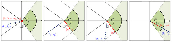
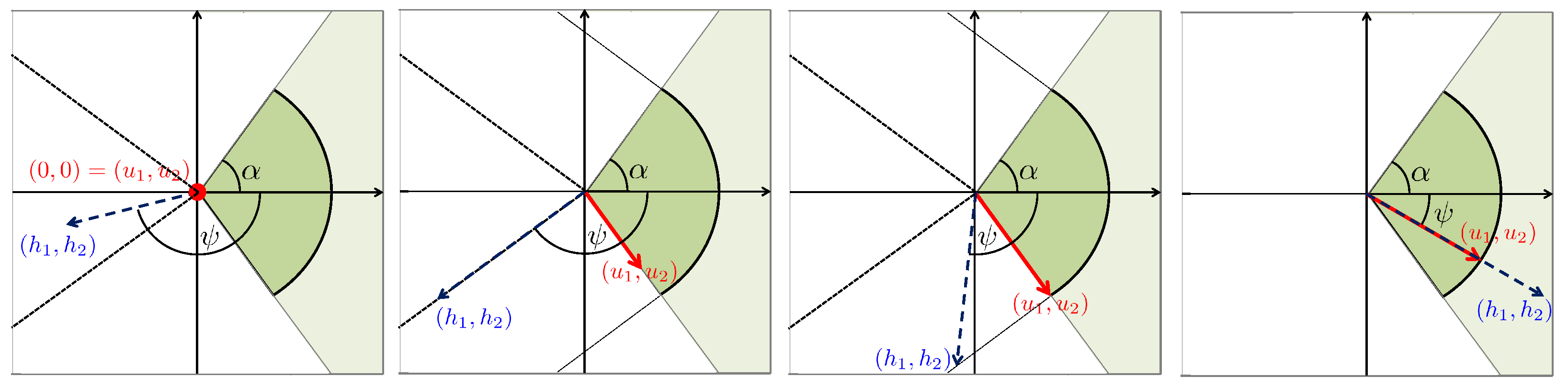
Note that the Pontryagin function $H_u$ can be seen as a scalar product of two vectors $(h_1,h_2)\in {\mathbb{R}}^2$ and $(u_1,u_2)\in U\subset {\mathbb{R}}^2$. From this point of view, the maximum condition has a clear geometric interpretation (see Figure 3).

Figure 3. The maximum condition.

Introduce polar coordinates in the planes $O{h}_1{h}_2$ and $O{u}_1{u}_2$:

$$\begin{array}{cc}{h}_1=\rho cos\psi ,h_2=\rho sin\psi ,\hfill & \psi \in (-\pi ,\pi ],\rho \ge 0;\hfill \\ u_1=rcos\varphi ,u_2=rsin\varphi ,\hfill & \varphi \in (0,\alpha ]\subset (0,\frac{\pi }{2}),r\in [0,1].\hfill \end{array}$$

For $\left|\psi \right|\in (\frac{\pi }{2}+\alpha ,\pi ]$, we have $H=0$ and $u_1=u_2=0$. In this case, we have trivial abnormal extremals.

For $\psi =\pm \left(\frac{\pi }{2}+\alpha \right)$, we have $H=0$, $u_1=rcos\alpha$, and $u_2=\pm rsin\alpha$. In this case, we have nontrivial abnormal extremals. We study them in detail in Section 5.2.

For $\rho =0$, we have $H=0$ for any $(u_1,u_2)\in U$. In this case, we have abnormal extremals. Since the Hamiltonian $H=0$ is constant along the extremals, the point $\rho =0$ can lie on a trivial or a nontrivial abnormal extremal that we listed in the two cases above. Further, we consider $\rho >0$.

For $\pm \psi \in (\alpha ,\frac{\pi }{2}+\alpha )$, we have $u_1=cos\alpha$, $u_2=\pm sin\alpha .$ In this case, we have $H=\rho cos\left(\alpha \mp \psi \right)>0$ and the normal extremals corresponding to the motion of a car along a circle of minimal possible radius, as we will show in Section 5.3.

For $\left|\psi \right|\le \alpha$, we have $u_1=cos\psi ,u_2=sin\psi$. In this case, we have $H=\rho >0$ that and the normal extremals corresponding to the motion of a car along sub-Riemannian geodesics, as we will show in Section 5.3.

5.2. Abnormal Case $H=0$

Trivial abnormal extremal control $(u_1,u_2)\equiv 0$ corresponds to the fixed point of the Hamiltonian system.

Nontrivial abnormal extremal controls are given by

$$u_1\left(t\right)=r\left(t\right)cos\alpha ,u_2\left(t\right)=sign\left(\psi \left(t\right)\right)r\left(t\right)sin\alpha ,\mathrm{where}0\le r\left(t\right)\le 1.$$

Proposition 1. 

If an admissible control $u\left(t\right)=(u_1,u_2)\left(t\right)\in U$, $t\in [0,T]$ is not arc length parameterized, i.e., there exists a positive measure set $\sigma \subset [0,T]$ such that $u_1^2\left(t\right)+u_2^2\left(t\right)<1$ for $t\in \sigma$, then $u\left(t\right)$ is not optimal.

Proof. 

Let $r\left(t\right)=\sqrt{u_1^2\left(t\right)+u_2^2\left(t\right)}$ for a given trajectory. Let us show that if $0\le r\left(t\right)<1$ on a set $\sigma \subset [0,T]$ of measure $\mu \left(\sigma \right)>0$, then the trajectory is not optimal. First, note that if $r\left(t\right)=0$ for all $t\in \sigma$, then this part of the trajectory is a fixed point. Staying in place is not optimal in a time minimization problem. Now, if $r\left(t\right)\in (0,1)$ for $t\in \sigma$, then one can reparametrize the trajectory with $\mathrm{d}s=r\left(t\right)\mathrm{d}t$. In this case, the support of the trajectory stays the same, new controls are also admissible, but the new motion time S becomes strictly less than the original one:

$$S={\int }_0^S\mathrm{d}s={\int }_0^{T}r\left(t\right)\mathrm{d}t={\int }_{\sigma }r\left(t\right)\mathrm{d}t+{\int }_{[0,T]\setminus \sigma }r\left(t\right)\mathrm{d}t<\mu \left(\sigma \right)+\mu ([0,T]\setminus \sigma )=T.$$

□

Further, we consider arclength parameterized abnormal extremals.

Theorem 3. 

Abnormal arclength parameterized extremal controls are piecewise constant

$$u_1\left(t\right)=cos\alpha ,u_2\left(t\right)=s_2\left(t\right)sin\alpha ,\mathrm{where}{s}_2\left(t\right)\in \{-1,1\},$$

with switching times (discontinuity points of $s_2\left(t\right)$) differing by $\frac{\pi }{sin\alpha }$. The corresponding trajectories are motions of a car along circular arcs of the minimal possible radius by angle π (except the first and the last arcs, which may have angles not greater than π).

Proof. 

Abnormal extremals satisfy the statements of the PMP: the maximum condition, the Hamiltonian system (11), and nontriviality condition $h_1^2\left(t\right)+h_2^2\left(t\right)+h_3^2\left(t\right)\ne 0$ for all $t\in [0,T]$.

From the maximum condition we have

$$h_1\left(t\right)=-R\left(t\right)sin\alpha ,h_2\left(t\right)=s_2\left(t\right)R\left(t\right)cos\alpha ,R\left(t\right)\ge 0.$$

(12)

Here, $s_2\left(t\right)=sign{h}_2\left(t\right)$.

The vertical part of the Hamiltonian system (11) is given by

$$\left\{\begin{array}{c}{\dot{h}}_1\left(t\right)=-s_2\left(t\right)sin\alpha h_3\left(t\right),\hfill \\ {\dot{h}}_2\left(t\right)=cos\alpha h_3\left(t\right),\hfill \\ {\dot{h}}_3\left(t\right)=s_2\left(t\right)sin\alpha h_1\left(t\right).\hfill \end{array}\right.$$

(13)

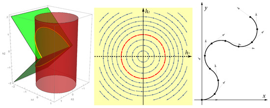
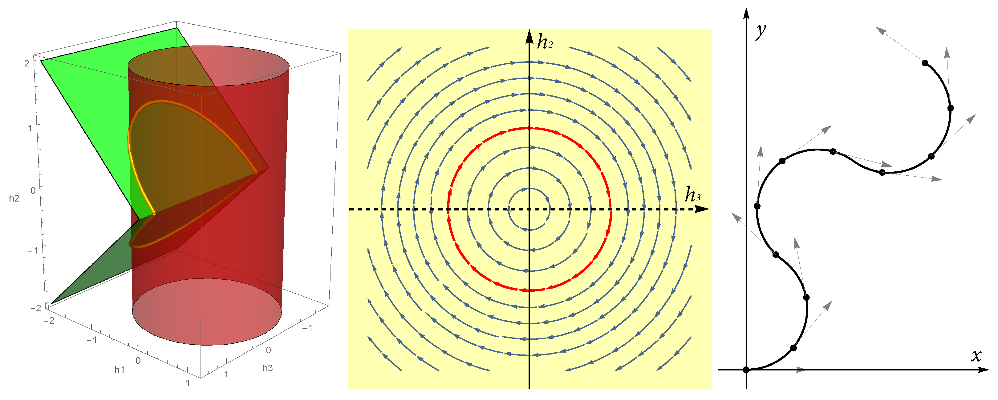
This system preserves the Hamiltonian $H=cos\alpha h_1+sin\alpha \left|h_2\right|$ and the Casimir $E=\frac{h_1^2+h_3^2}{2}$ (see Figure 4). Since $H=0$ for abnormal extremals, the nontriviality condition implies $E>0$.

Figure 4. Abnormal case. (Left) Level surfaces of the Hamiltonian $H=0$ (in green) and the Casimir $E>0$ (in red). (Center) Phase portrait on the surface $H=0$. (Right) An abnormal extremal trajectory.

Denote $a=\sqrt{2E}>0$. Let $h_1=acos\phi$, $h_3=asin\phi$, and $c=h_2$, where $\phi \in [\frac{\pi }{2},\frac{3\pi }{2}]$ as we have $h_1\le 0$ (see (12)). System (13) reads

$$\left\{\begin{array}{c}\dot{\phi }\left(t\right)=sin\alpha s_2\left(t\right),\hfill \\ \dot{c}\left(t\right)=acos\alpha sin\phi \left(t\right).\hfill \end{array}\right.$$

If $c\left(t_1\right)=0$, for some $t_1\in [0,T]$, then $H=0$ implies $h_1\left(t_1\right)=0$ and $\phi \left(t_1\right)=\pi \pm \frac{\pi }{2}$. Thus, $sin\phi \left(t_1\right)=\pm 1$ and from the second equation of the system, we have $\dot{c}\left(t\right)\ne 0$ for $[t_1-\epsilon ,t_1+\epsilon ]$ for sufficiently small $\epsilon >0$. Thus, the function $c\left(t\right)$ changes its sign in a neighborhood of $t_1$. We see that $t_1$ is an isolated point where $c\left(t\right)$ changes its sign.

If $c\left(t\right)\ne 0$, then $s_2\left(t\right)=signc\left(t\right)$ (see (12)). The extremal control $u_2\left(t\right)=signc\left(t\right)sin\alpha$ is piecewise constant with interval between switchings $\Delta t=t_2-t_1=\frac{\pi }{sin\alpha }$, as it follows from the first equation of the system with boundary values $\phi \left(t_1\right)=\pi \pm \frac{\pi }{2}$, $\phi \left(t_2\right)=\pi \mp \frac{\pi }{2}$.

The corresponding trajectory of the horizontal part of (11) is easy to find by direct integration. For time intervals between switchings, the point $\left(x\right(t),y(t\left)\right)$ moves along the circular arc with increments of angle $\Delta \theta =\pm sin\alpha \Delta t=\pm \pi$. □

5.3. Normal Case $H>0$

In this section, we provide a qualitative analysis of the dynamics in the normal case $H>0$. Note that the normal case appears iff $\left|\psi \right|<\frac{\pi }{2}+\alpha$. In the normal case, we set the Hamiltonian value $H=1$ without loss of generality (see [20]).

The vertical part has the first integrals: the Hamiltonian

$$1=H=\left\{\begin{array}{cc}{h}_{1}cos\alpha +\left|h_2\right|sin\alpha ,\hfill & \mathrm{for}\alpha <\left|\psi \right|<\frac{\pi }{2}+\alpha ,\hfill \\ \sqrt{h_1^2+h_2^2},\hfill & \mathrm{for}\left|\psi \right|\le \alpha ,\hfill \end{array}\right.$$

(14)

and the Casimir

$$E=\frac{h_1^2}{2}+\frac{h_3^2}{2}.$$

(15)

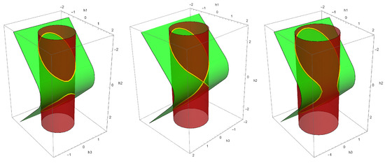
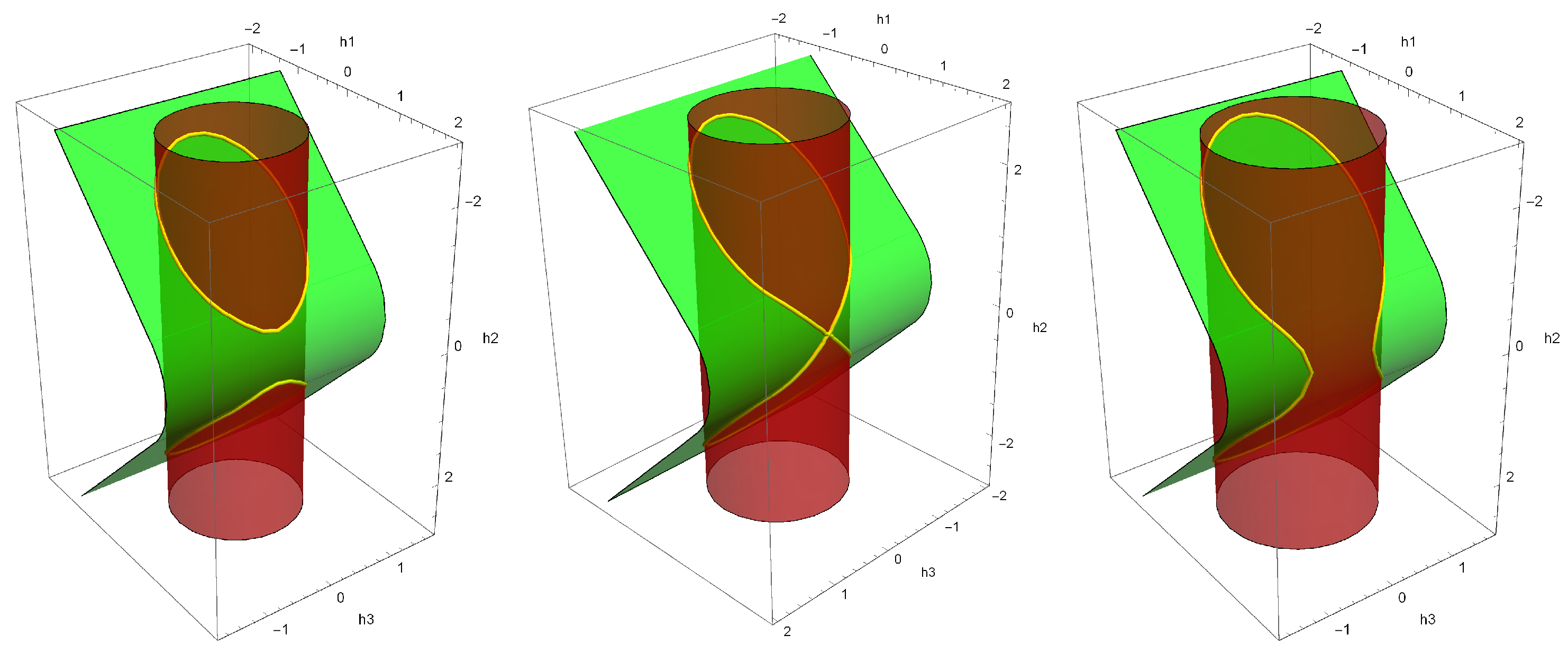
In Figure 5, we show variants of the mutual arrangement of the level surface of the Hamiltonian $H=1$, which consists of two half-planes glued with a segment of the cylinder, and the level surface of the Casimir $E\ge 0$, which is a cylinder.

Figure 5. Level surfaces of the Hamiltonian H (in green) and the Casimir E (in red). (Left) $E<\frac{1}{2}$. (Center) $E=\frac{1}{2}$. (Right) $E>\frac{1}{2}$.

For the description of the phase portrait of the vertical part, we use techniques of convex trigonometry [26]. The polar set to U is

$$\begin{array}{ccc}& & U^o=\left\{\left.(h_1,h_2)\in {\mathbb{R}}^{2\ast }\right|u_1{h}_1+u_2{h}_2\le 1,(u_1,u_2)\in U\right\}=\hfill \\ & & \left\{\left(h_1,h_2\right)=(\rho cos\psi ,\rho sin\psi )\left|\begin{array}{c}\mathrm{for}\left|\psi \right|\le \alpha :\sqrt{h_1^2+h_2^2}\le 1,\hfill \\ \mathrm{for}\alpha <\psi <\alpha +\frac{\pi }{2}:h_{1}cos\alpha +h_{2}sin\alpha \le 1,\hfill \\ \mathrm{for}-\alpha -\frac{\pi }{2}<\psi <-\alpha :h_{1}cos\alpha -h_{2}sin\alpha \le 1\hfill \end{array}\right.\right\}.\hfill \end{array}$$

The corresponding functions of convex trigonometry are

$$\begin{array}{ccc}& & {cos}_{U^o}{\varphi }^o=\left\{\begin{array}{cc}cos{\varphi }^o,\hfill & \mathrm{for}|{\varphi }^o|\le \alpha ,\hfill \\ cos\alpha -({\varphi }^o-\alpha )sin\alpha ,\hfill & \mathrm{for}|{\varphi }^o|>\alpha ,\hfill \end{array}\right.\hfill \\ & & {sin}_{U^o}{\varphi }^o=\left\{\begin{array}{cc}sin{\varphi }^o,\hfill & \mathrm{for}|{\varphi }^o|\le \alpha ,\hfill \\ \pm (sin\alpha +({\varphi }^o-\alpha )cos\alpha ),\hfill & \mathrm{for}|{\varphi }^o|>\alpha ,\hfill \end{array}\right.\hfill \end{array}$$

where $\pm =sign\left({\varphi }^o\right)$.

Along the extremal trajectories, we have

$$\begin{array}{c}\hfill u_1=cos\varphi ,u_2=sin\varphi ,h_1={cos}_{U^o}{\varphi }^o,h_2={sin}_{U^o}{\varphi }^o.\end{array}$$

Denote $K\left({\varphi }^o\right)=\frac{1}{2}{cos}_{U^o}^2{\varphi }^o$. The Casimir E can be seen as a total energy integral (sum of potential and kinetic energy)

$$E=\frac{h_1^2}{2}+\frac{h_3^2}{2}=\frac{h_3^2}{2}+K\left({\varphi }^o\right)$$

of conservative system with one degree of freedom [27]

$$\dot{{\varphi }^o}=h_3,{\dot{h}}_3=-K^{\prime }\left({\varphi }^o\right).$$

(16)

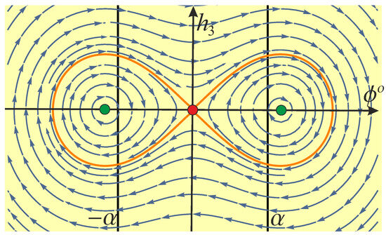
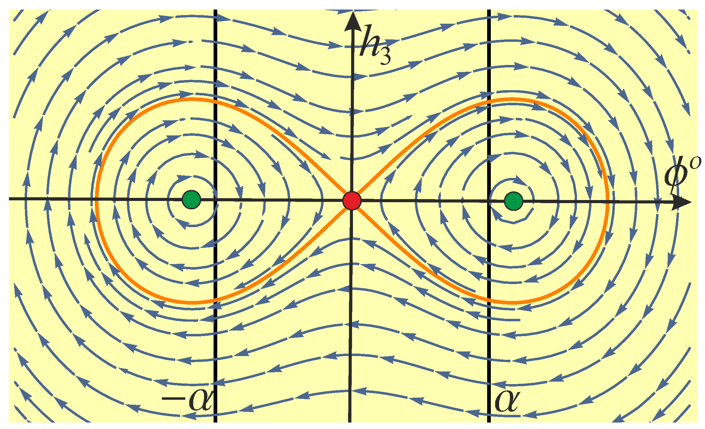
The phase portrait of this system is depicted in Figure 6.

Figure 6. The phase portrait on the level surfaces of the Hamiltonian $H=1$.

Analyzing the phase portrait of (16), we conclude:

$E=0\Rightarrow ({\varphi }^o,h_3)\equiv (\pm (\alpha +cot\alpha ),0)$ is stable equilibrium;

$E\in (0,\frac{1}{2})\cup (\frac{1}{2},+\infty )\Rightarrow$ the trajectory $({\varphi }^o,h_3)\left(t\right)$ is periodic;

$E=\frac{1}{2}\Rightarrow$ either $({\varphi }^o,h_3)\equiv (0,0)$ is unstable equilibrium or $({\varphi }^o,h_3)\left(t\right)$ is a separatrix of the saddle point.

6. Explicit Expression for Normal Extremals

6.1. Stratification of the Hamiltonian System Adjoint Variables Domain

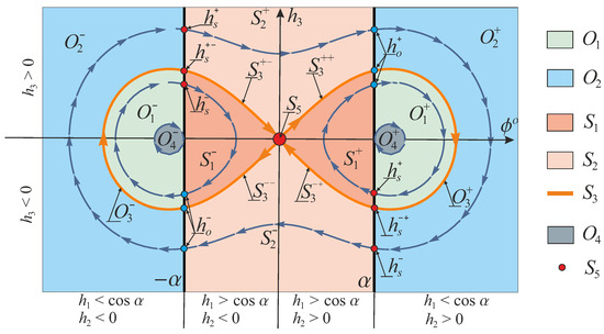
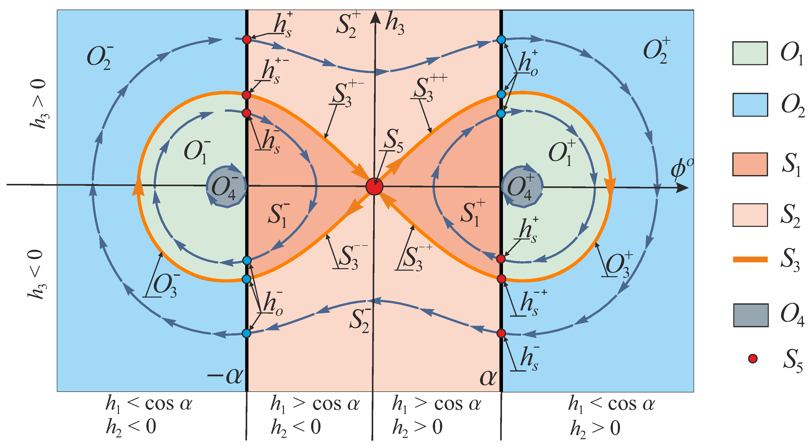
In this section, we derive explicit expressions for the normal extremals. To this end, we stratify the domain of adjoint variables $h_1$, $h_2$, and $h_3$ into five subdomains and introduce the coordinates $(\xi ,k)$ that rectify the phase portrait of the vertical part in each subdomain. Next, we integrate the horizontal part and derive explicit expressions for the extremal trajectories. This method was applied for the construction of optimal synthesis in several optimal control problems [28].

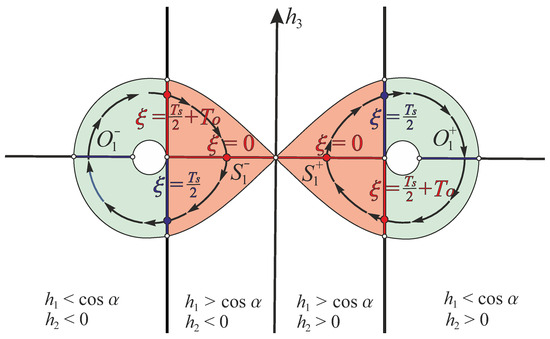
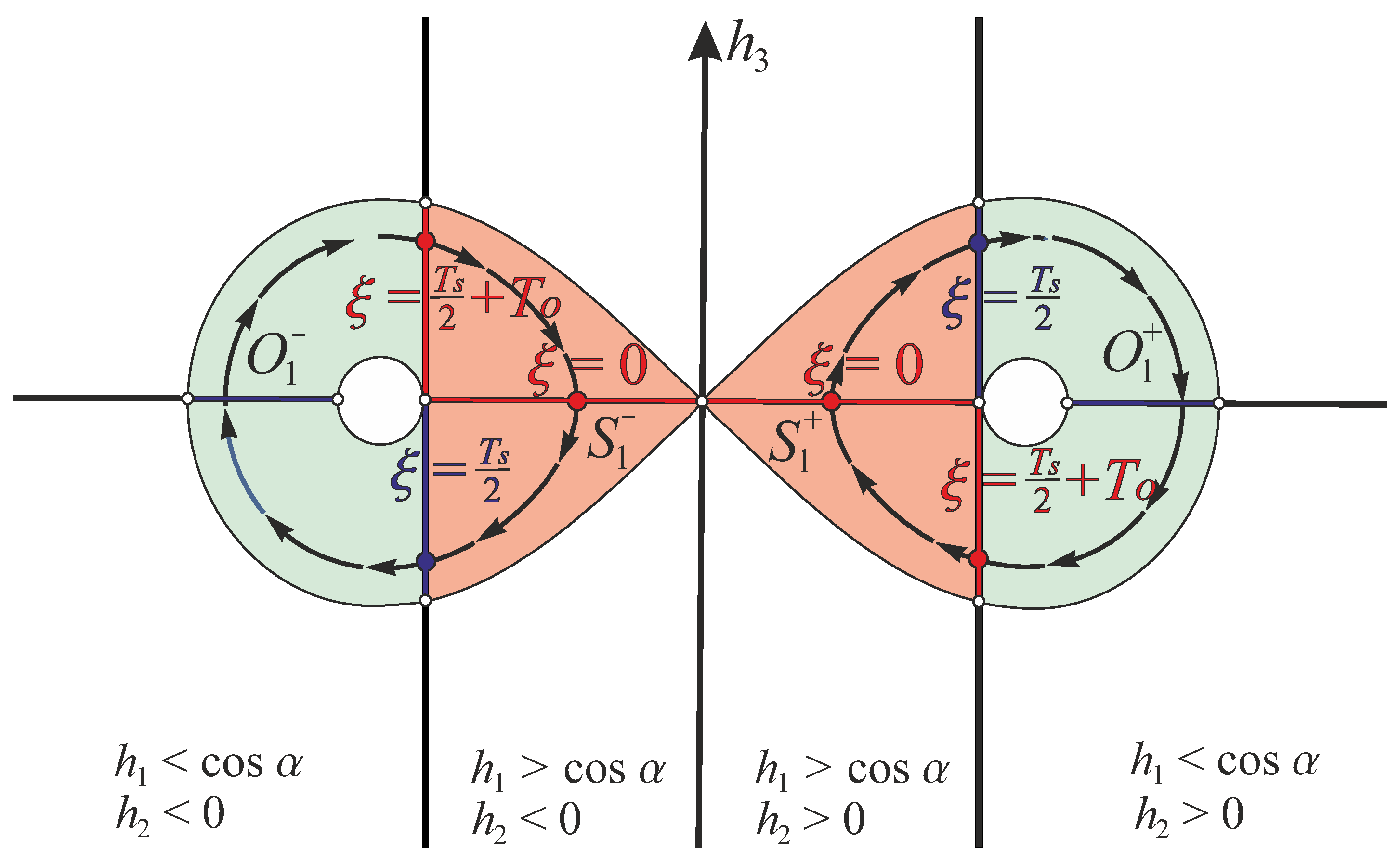
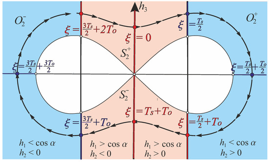
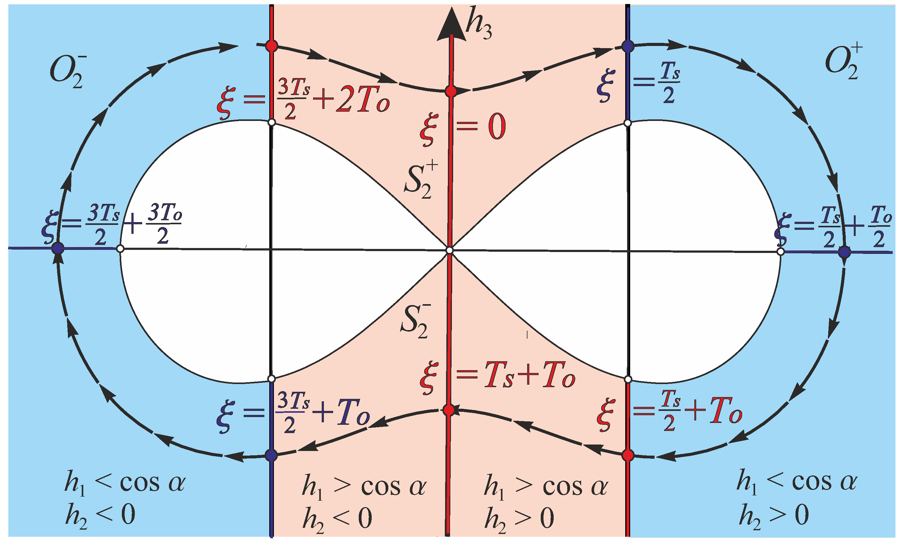
In Figure 7, we stratify the domain of the vertical part with respect to the value of the Casimir E, the value of ${\varphi }^o$, and the sign $s_i=sign{h}_i$, $i=2,3$. From the analysis in the previous section, we know that there are two generic types of motion: $|{\varphi }^0|<\alpha$ and $|{\varphi }^0|>\alpha$, which are equivalent to $h_1>cos\alpha$ and $h_1<cos\alpha$, respectively. We denote by the letter S the domain with the first type of motion and by O the domain with the second type of motion. Such notions are motivated by S — sub-Riemannian, and O — circle, as we will show next that the corresponding extremal trajectory (solution to the horizontal part) is given by arcs of sub-Riemannian geodesics in ${SE}_2$ [4] and arcs of circular extremals (which correspond to motion of a car along circles of minimal possible radius).

Figure 7. Stratification of the domain of the vertical part.

Denote $\mathcal{E}=\sqrt{2E}$. There are five qualitative types of normal extremal trajectories:

1.

Arcs of noninflectional sub-Riemannian geodesics in ${SE}_2$, joined by arcs of the circular extremals, when $cos\alpha <\mathcal{E}<1$ (the subdomain $S_1^{\pm }\cup O_1^{\pm }$; $\pm =sign{h}_2$);

2.

Arcs of inflectional sub-Riemannian geodesics in ${SE}_2$ joined by arcs of the circular extremals, when $\mathcal{E}>1$ (the subdomain $S_2^{\pm }\cup O_2^{\pm }$; here, $\pm =sign{h}_3$ in the S-domain, and $\pm =sign{h}_2$ in the O-domain);

3.

Arcs of the separatrix sub-Riemannian geodesics in ${SE}_2$ joined by an arc of the circular extremal, when $\mathcal{E}=1$ and $h_1<1$ (the subdomain $S_3^{\pm \pm }\cup O_3^{\pm }$; here, $(\pm ,\pm )=(sign{h}_3,sign{h}_2)$ in the S-domain, and $\pm =sign{h}_2$ in the O-domain);

4.

The circular extremals, when $\mathcal{E}\le cos\alpha$ (the subdomains $O_4^{\pm }$; here, $\pm =sign{h}_2$ correspond to the motion of the car clockwise or counterclockwise);

5.

The straight extremal (the ray), when $\mathcal{E}=1$ and $h_1=1$ (the subdomain $S_5$).

Next, we derive explicit formulas for the extremals in each case. In order to avoid difficulties in the interpretation of formulas of convex trigonometry, which appeared very useful for qualitative analysis of the Hamiltonian system in the previous section, we return to the classical coordinates $(h_1,h_2,h_3)\in C\subset {\mathbb{R}}^3$, where the vertical part (16) takes the form

$$\left\{\begin{array}{c}{\dot{h}}_1=-h_2{h}_3,\hfill \\ {\dot{h}}_2=h_1{h}_3,\hfill \\ {\dot{h}}_3=h_2{h}_1,\hfill \end{array}\right.\mathrm{for}{h}_1>cos\alpha ;\left\{\begin{array}{c}{\dot{h}}_1=-s_{2}sin\alpha h_3,\hfill \\ {\dot{h}}_2=cos\alpha h_3,\hfill \\ {\dot{h}}_3=s_{2}sin\alpha h_1,\hfill \end{array}\right.\mathrm{for}{h}_1<cos\alpha ;$$

(17)

where $s_2=sign{h}_2$. The extremal controls are given by

$$(u_1,u_2)=(h_1,h_2),\mathrm{for}{h}_1>cos\alpha ;(u_1,u_2)=(cos\alpha ,s_{2}sin\alpha ),\mathrm{for}{h}_1<cos\alpha ;$$

(18)

and the horizontal part is given by

$$\left\{\begin{array}{c}\dot{x}=u_{1}cos\theta ,\hfill \\ \dot{y}=u_{1}sin\theta ,\hfill \\ \dot{\theta }=u_2.\hfill \end{array}\right.$$

(19)

Note that for $h_1>cos\alpha$, System (17)–(19) coincides with the system for sub-Riemannian geodesics in ${SE}_2$ [4]. Thus, the solutions in the S-domains are given by arcs of sub-Riemannian geodesics. Denote by $\sigma :\mathbb{R}\times C\to {SE}_2:(t,h^0)\mapsto \sigma (t,h^0)$ the flow from Id along the sub-Riemannian geodesic with the initial covector $h^0\in C$. The exact formula for the operator $\sigma$ in the different domains is presented in the subsections below.

For $h_1<cos\alpha$, System (17)–(19) is easily integrated, and the solutions are given by arcs of circles of radius $cot\alpha$, which is the minimal possible turning radius for the car model. Denote by $\omega :\mathbb{R}\times C\to {SE}_2:(t,h^0)\mapsto \omega (t,h^0)$ the corresponding flow from Id:

$$\omega (t,h^0)=\left(cot\alpha sin(tsin\alpha ),s_{2}cot\alpha (1-cos(tsin\alpha )),s_{2}tsin\alpha \right).$$

(20)

The case $h_1=cos\alpha$ is joined to the case $h_1>cos\alpha$ when $s_2{s}_3<0$, and joined to the case $h_1<cos\alpha$, when $s_2{s}_3>0$ (see Figure 7). Here, $s_2=sign{h}_2$, and $s_3=sign{h}_3$.

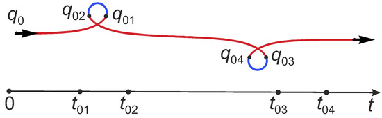
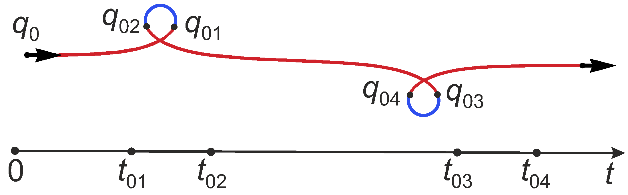
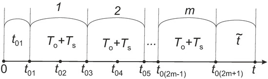
To obtain a general solution for the horizontal part we separate the timeline by the intervals, in which the S or the O mode holds. We denote by $t_{0i}$, $i\in \mathbb{N}$, the instances of time when the dynamics switches (see Figure 8). Denote by $h^{0i}\in C$ the corresponding value of the adjoint covector, and by $q_{0i}=q\left(t_{0i}\right)\in {SE}_2$ the corresponding point of the extremal trajectory. Due to left-invariance (see Remark 1), the arc of the trajectory starting from $q_{0i}$ is given by

$$\begin{array}{cc}q\left(t\right)=L_{q_{0i}}\sigma (t-t_{0i},h^{0i})=q_{0i}·\sigma (t-t_{0i},h^{0i}),\hfill & \mathrm{in}\mathrm{S-domain},\hfill \\ q\left(t\right)=L_{q_{0i}}\omega (t-t_{0i},h^{0i})=q_{0i}·\omega (t-t_{0i},h^{0i}),\hfill & \mathrm{in}\mathrm{O-domain}.\hfill \end{array}$$

(21)

Figure 8. Timeline with indicated instances of switching and the corresponding trajectory.

6.2. The Domain $cos\alpha <\mathcal{E}<1$

Here, we consider the case when the initial covector $h^0$ belongs to the subdomain $S_1^{\pm }\cup O_1^{\pm }$, where $\pm =sign{h}_2=:s_2$. Notice that in this case, the trajectory of the vertical part is periodic, and $s_2$ is constant (see Figure 7). Denote the period by $T_o+T_s$, where $T_o$ is the full time of motion in the O-domain, and $T_s$ is the full time of motion in the S-domain.

Denote $k:=\mathcal{E}$. Introduce the coordinates $(\xi ,k)\in [-\frac{T_s}{2},\frac{T_s}{2}+T_o]\times (cos\alpha ,1)$ (see Figure 9). Here, $\xi$ is periodic with the period $T_s+T_o$.

Figure 9. Rectified coordinates in the domain $cos\alpha <\mathcal{E}<1$.

For $h^0=(h_{10},h_{20},h_{30})$ in $S_1^{\pm }$, where $\pm =s_2=sign{h}_{20}$:

$$\left\{\begin{array}{c}{h}_1=ksn({\xi }_c+\xi ),\hfill \\ h_2=s_{2}dn({\xi }_c+\xi ),\hfill \\ h_3=-s_{2}ksn({\xi }_c+\xi ),\hfill \end{array}\right.$$

(22)

where ${\xi }_c=K$, $\xi \in \left[-\frac{T_s}{2},\frac{T_s}{2}\right]$. The time $T_s$ of the full motion is computed as

$$T_s=2\left(F\left(arg\left(-\sqrt{k^2-{cos}^2\alpha }+\mathbf{i}cos\alpha \right)\right)-K\right),\mathrm{where}arg\in \left(\frac{\pi }{2},\pi \right),$$

(23)

and the initial value ${\xi }_0$ is expressed via $h^0$ as follows:

$${\xi }_0=F\left(arg\left(-s_2{h}_{30}+\mathbf{i}{h}_{10}\right)\right)-{\xi }_c,\mathrm{where}arg\in (0,\pi ).$$

Here, sn, cn, and dn are Jacobi elliptic functions; F is the elliptic integral of the first kind; and $K=F\left(\frac{\pi }{2}\right)$ is the complete elliptic integral of the first kind.

For $h^0=(h_{10},h_{20},h_{30})$ in $O_1^{\pm }$, where $\pm =s_2=sign{h}_{20}$:

$$\left\{\begin{array}{c}{h}_1=kcos(sin\alpha ({\xi }_c+\xi )),\hfill \\ h_2=\frac{s_2}{sin\alpha }\left(1-kcos\alpha cos(sin\alpha ({\xi }_c+\xi ))\right),\hfill \\ h_3=s_{2}ksin(sin\alpha ({\xi }_c+\xi )),\hfill \end{array}\right.$$

(24)

where ${\xi }_c=\frac{\phi }{sin\alpha }-\frac{T_s}{2}$, $\xi \in \left[\frac{T_s}{2},\frac{T_s}{2}+T_o\right]$. The time $T_o$ of the full motion is computed as

$$T_o=\frac{2}{sin\alpha }\left(\pi -\phi \right),\mathrm{where}\phi =arg\left(cos\alpha +\mathbf{i}\sqrt{k^2-{cos}^2\alpha }\right)\in \left(0,\frac{\pi }{2}\right),$$

(25)

and the initial value ${\xi }_0$ is expressed via $h^0$ as follows:

$${\xi }_0=arg\left(h_{10}+\mathbf{i}{s}_2{h}_{30}\right)/sin\alpha -{\xi }_c,\mathrm{where}arg\in \left(0,\frac{\pi }{2}\right)\cup \left(\frac{3\pi }{2},2\pi \right).$$

The direct computation shows that (17) is rectified in the coordinates $(\xi ,k)$:

$$\xi \left(t\right)={\xi }_t={\xi }_0+t,k=const.$$

Remark 5. 

There is a symmetry between the solutions for $s_2=1$ and $s_2=-1$: the substitution $(h_1,h_2,h_3)\to (h_1,-h_2,-h_3)$ translates a trajectory in $S_1^{\pm }\cup O_1^{\pm }$ to the trajectory in $S_1^{\mp }\cup O_1^{\mp }$.

Remark 6. 

The values $T_s$ and $T_o$ are computed as the minimal positive time instances when

$$\begin{array}{cc}\left(h_1\left(0\right),h_3\left(0\right)\right)=\left(cos\alpha ,-\sqrt{k^2-h_1^2\left(0\right)}\right),\hfill & \left(h_1\left(T_s\right),h_3\left(T_s\right)\right)=\left(cos\alpha ,\sqrt{k^2-h_1^2\left(0\right)}\right),\hfill \\ \left(h_1\left(0\right),h_3\left(0\right)\right)=\left(cos\alpha ,\sqrt{k^2-h_1^2\left(0\right)}\right),\hfill & \left(h_1\left(T_o\right),h_3\left(T_o\right)\right)=\left(cos\alpha ,-\sqrt{k^2-h_1^2\left(0\right)}\right).\hfill \end{array}$$

Now we integrate the horizontal part and find the exact expression for the extremal trajectories. Recall that in the O-domain, the extremal trajectories $q\left(t\right)=\omega (t,h^0)$ are given by arcs of the circles (20), and in the S-domain, the extremal trajectories $q\left(t\right)=\sigma (t,h^0)$ are given by arcs of sub-Riemannian geodesics. Exact formulas for the sub-Riemannian geodesics are found in [4]. In our notation, they read as:

$$\begin{array}{c}\sigma (t,h^0)=\left(x\left(t\right),y\left(t\right),\theta \left(t\right)\right),\hfill \\ x\left(t\right)=\frac{1}{k}\left(s\beta \left(t-E\left(am\left({\xi }_c+{\xi }_t\right)\right)+E\left(\beta \right)\right)-c\beta \left(dn\left({\xi }_c+{\xi }_t\right)-\sqrt{1-k^{2}s{\beta }^2}\right)\right),\hfill \\ y\left(t\right)=\frac{s_2}{k}\left(c\beta \left(t-E\left(am\left({\xi }_c+{\xi }_t\right)\right)+E\left(\beta \right)\right)+s\beta \left(dn\left({\xi }_c+{\xi }_t\right)-\sqrt{1-k^{2}s{\beta }^2}\right)\right),\hfill \\ \theta \left(t\right)=s_2\left(-\beta +am\left({\xi }_c+{\xi }_t\right)\right),\hfill \end{array}$$

(26)

where

$$\beta =am\left({\xi }_0+{\xi }_c\right),s\beta =sin\beta =sn\left({\xi }_0+{\xi }_c\right),c\beta =cos\beta =cn\left({\xi }_0+{\xi }_c\right).$$

Here, am, sn, cn, and dn are Jacobi elliptic functions, and E is the elliptic integral of the second kind.

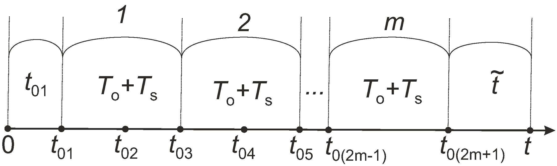
To obtain a general solution for the horizontal part, we separate the timeline by the intervals

$$[0,t]=[0,t_{01})\cup [t_{01},t_{02})\cup [t_{02},t_{03})\cup \dots \cup [t_{0(2m-1)},t_{0(2m+1)})\cup [t_{0(2m+1)},t_{0(2m+1)}+\tilde{t}],$$

in which the S or the O mode holds (see Figure 10). Here, we have

$$\tilde{t}=t-t_{01}-m\left(T_o+T_s\right),m=\left[\frac{t-t_{01}}{T_o+T_s}\right],t_{01}=min\left\{t>0|h_1\left(t\right)=cos\alpha \right\},$$

(27)

where the square brackets denote the integer part.

Figure 10. Timeline for the trajectory with indicated instances of switches.

Denote

$$h_o^{\pm }=\left(cos\alpha ,\pm sin\alpha ,\pm \sqrt{k^2-{cos}^2\alpha }\right),h_s^{\pm }=\left(cos\alpha ,\pm sin\alpha ,\mp \sqrt{k^2-{cos}^2\alpha }\right)$$

(28)

the initial covector for the full arc of O and S segment of the extremals (see Figure 7), and

$$q_{\omega }^{\pm }=\omega (T_o,h_o^{\pm }),q_{\sigma }^{\pm }=\sigma (T_s,h_s^{\pm })$$

(29)

the end point of the corresponding extremal trajectory.

Now we obtain the resulting formula for the extremal trajectories by usage of (21).

Theorem 4. 

For $h^0\in S_1^{\pm }$, the corresponding extremal trajectory is given by

$$q\left(t\right)=\left\{\begin{array}{cc}\sigma (t,h^0),\hfill & \mathit{for}t\in [0,t_{01}),\hfill \\ q_{01}·{\left(q_{\sigma }^{\pm }·q_{\omega }^{\pm }\right)}^m·\omega \left(\tilde{t},h_o^{\pm }\right),\hfill & \mathit{for}0\le \tilde{t}<T_o,\hfill \\ q_{01}·{\left(q_{\sigma }^{\pm }·q_{\omega }^{\pm }\right)}^m·q_{\omega }^{\pm }·\sigma \left(\tilde{t}-T_o,h_s^{\pm }\right),\hfill & \mathit{for}{T}_o\le \tilde{t}<T_o+T_s,\hfill \end{array}\right.$$

where $q_{01}=\sigma \left(t_{01},h^0\right)$.

For $h^0\in O_1^{\pm }$, the corresponding extremal trajectory is given by

$$q\left(t\right)=\left\{\begin{array}{cc}\omega (t,h^0),\hfill & \mathit{for}t\in [0,t_{01}),\hfill \\ q_{01}·{\left(q_{\sigma }^{\pm }·q_{\omega }^{\pm }\right)}^m·\sigma \left(\tilde{t},h_s^{\pm }\right),\hfill & \mathit{for}0\le \tilde{t}<T_s,\hfill \\ q_{01}·{\left(q_{\sigma }^{\pm }·q_{\omega }^{\pm }\right)}^m·q_{\sigma }^{\pm }·\omega \left(\tilde{t}-T_s,h_o^{\pm }\right),\hfill & \mathit{for}{T}_s\le \tilde{t}<T_o+T_s,\hfill \end{array}\right.$$

where $q_{01}=\omega \left(t_{01},h^0\right)$.

For both cases, the operators σ and ω are defined by (26) and (20); the values $T_s$ and $T_o$ are defined by (23) and (25); the values $\tilde{t}$, m, and $t_{01}$ are defined by (27); and the initial covectors $h_o^{\pm }$ and $h_s^{\pm }$ and the corresponding end points $q_{\sigma }^{\pm }$ and $q_{\omega }^{\pm }$ are defined by (28) and (29).

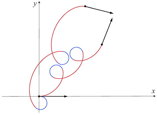
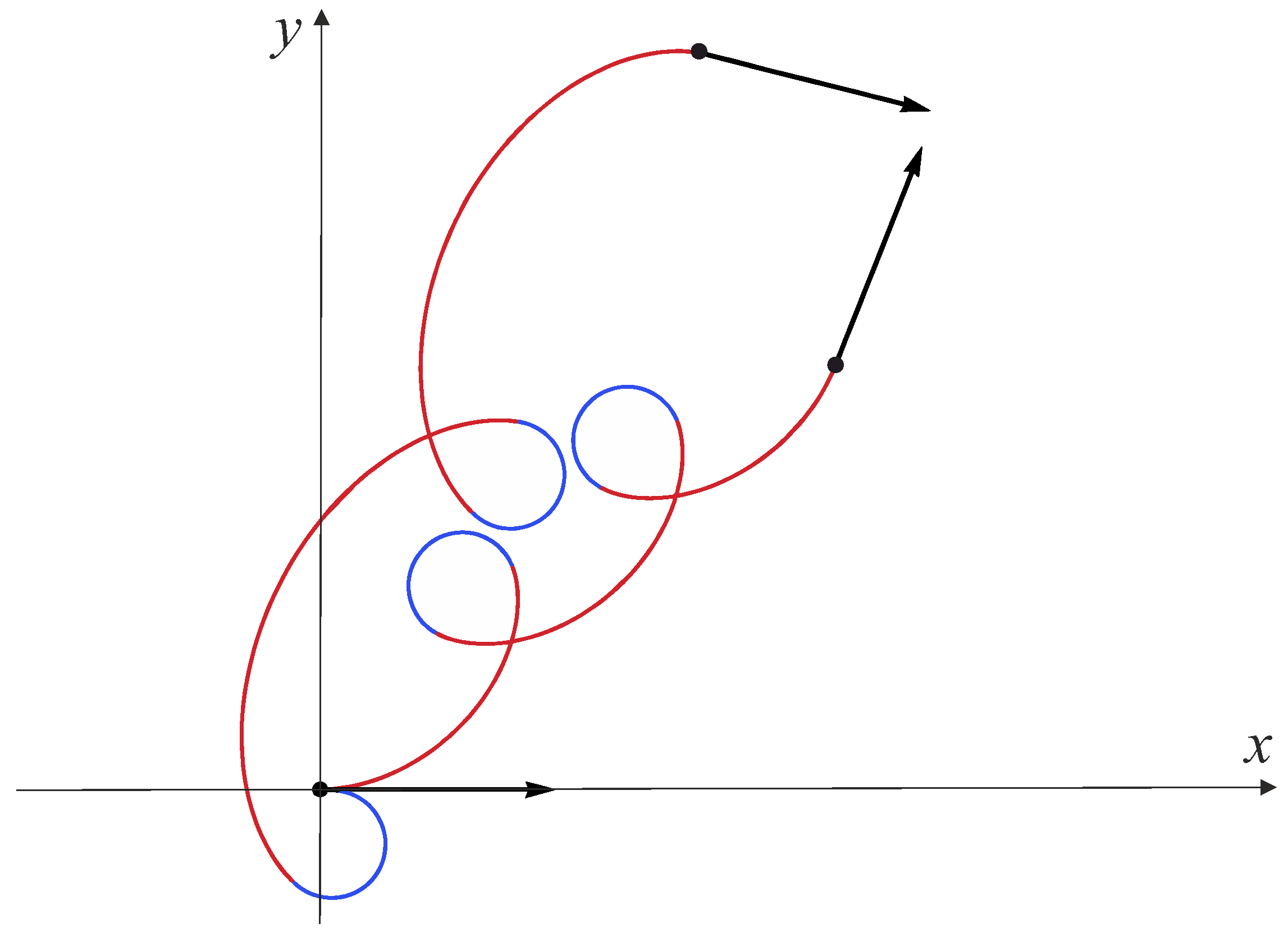
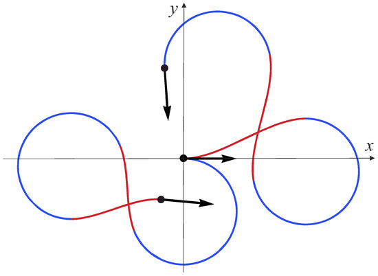
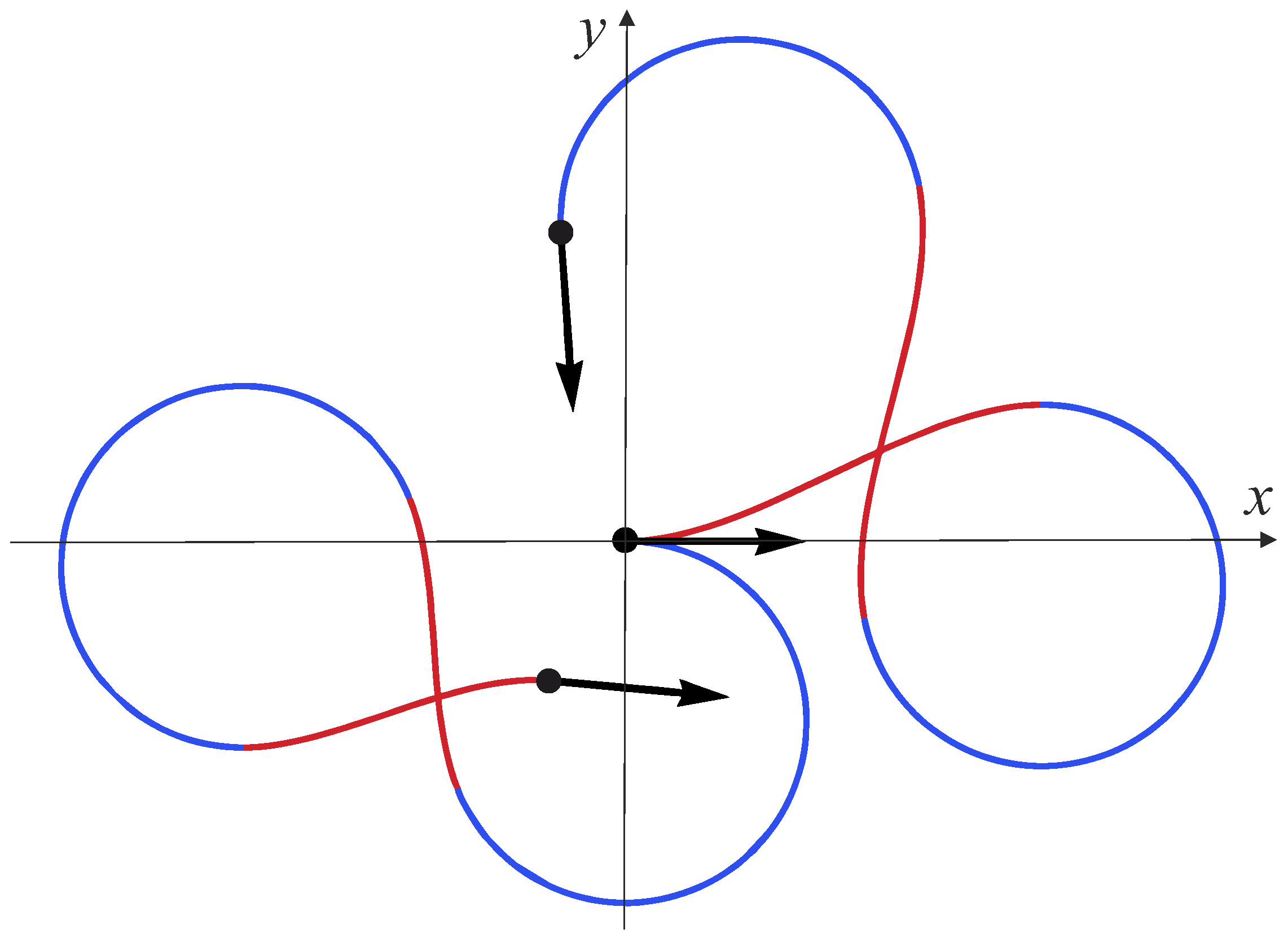
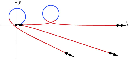
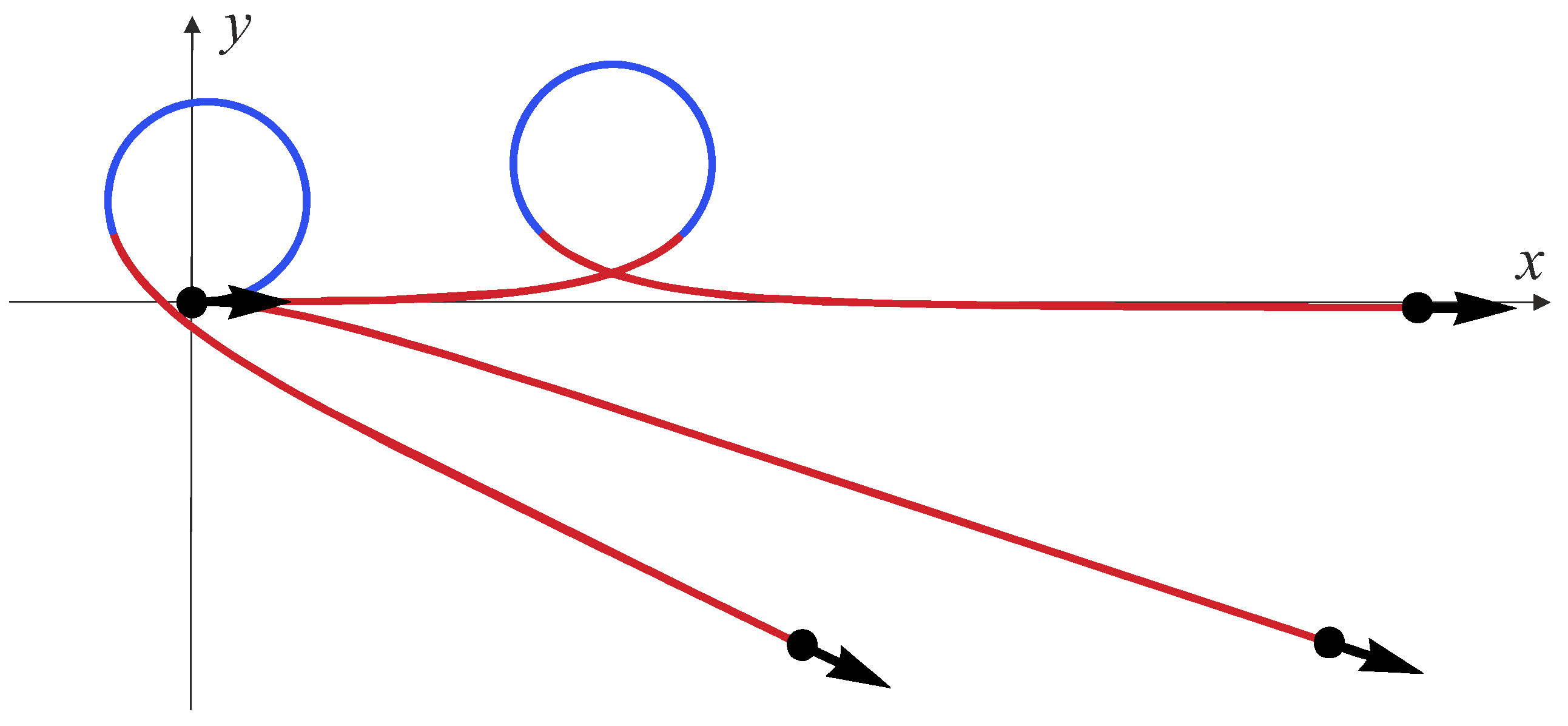
In Figure 11, we show an example of the extremal trajectories in the domain $S_1^{\pm }\cup O_1^{\pm }$.

Figure 11. Two extremal trajectories in $S_1^{\pm }\cup O_1^{\pm }$ with $\alpha =\frac{3\pi }{7}$ for $t\in [0,15.4]$: for $h^0=(0.32,-0.85,-0.66)$ and $h^0=(0.52,0.85,-0.46)$. The sub-Riemannian arcs are depicted in red, and arcs of the circles are depicted in blue.

Remark 7. 

The power of an element $q\in {SE}_2$ is defined as

$$q^m=\left\{\begin{array}{cc}Id,\hfill & \mathit{for}m=0,\hfill \\ \stackrel{m\mathrm{times}}{\overbrace{q·\dots ·q}},\hfill & \mathit{for}m\ge 1.\hfill \end{array}\right.$$

6.3. The Domain $\mathcal{E}>1$

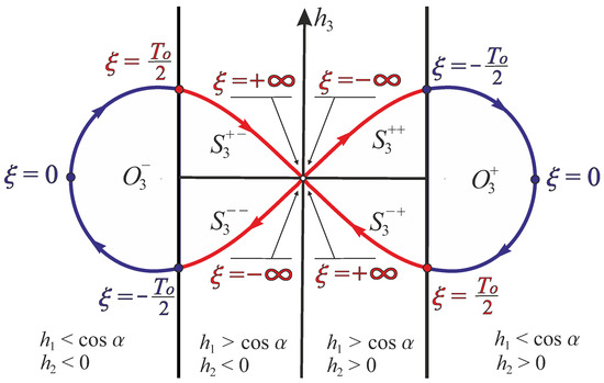
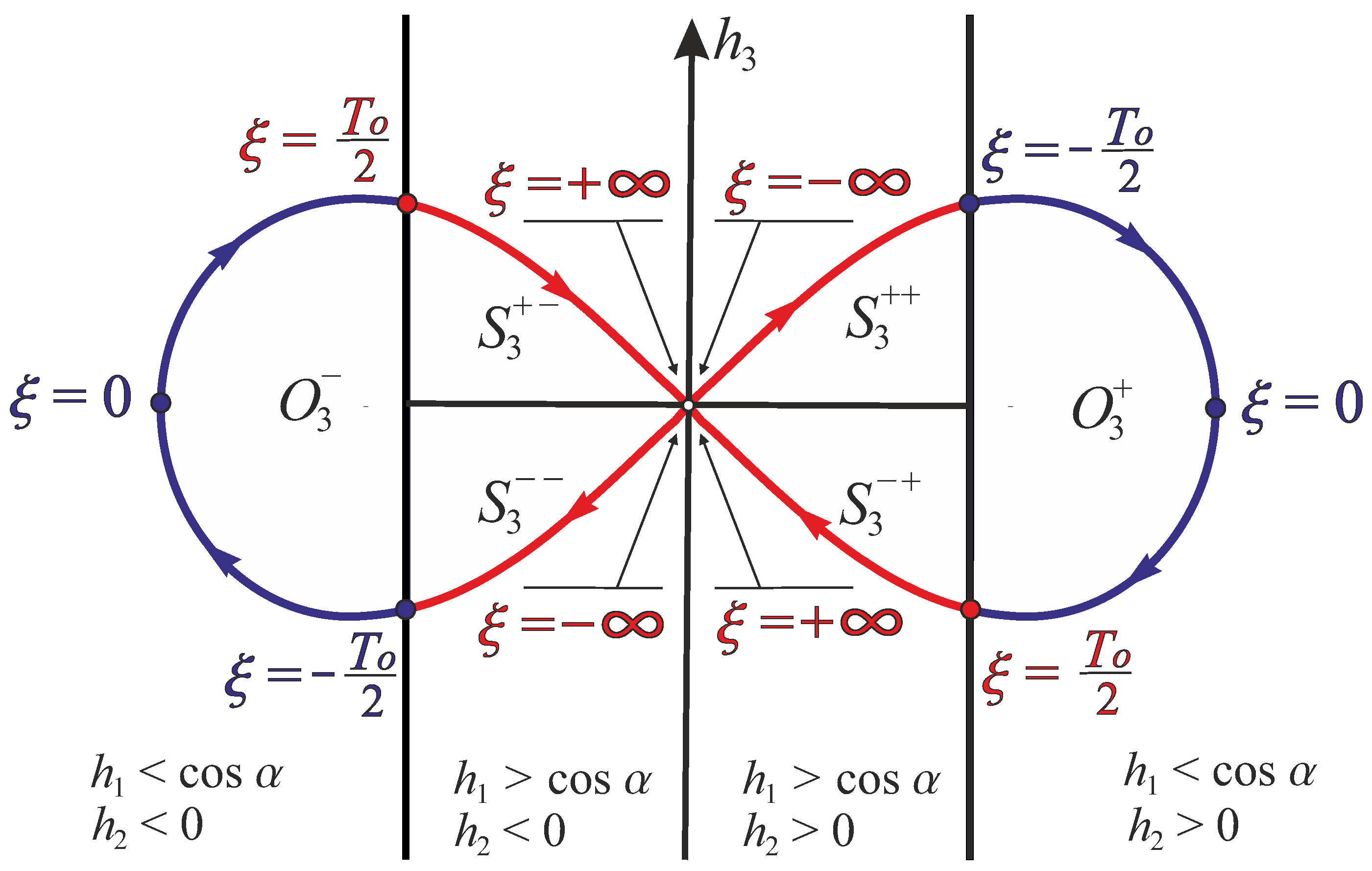
Here, we consider the case when the initial covector $h^0$ belongs to the subdomain $S_2^{\pm }\cup O_2^{\pm }$, where $\pm =sign{h}_3=:s_3$ in the S-domain, and $\pm =sign{h}_2=:s_2$ in the O-domain. Notice that in this case, the trajectory of the vertical part is periodic (see Figure 7). Denote the period by $2(T_o+T_s)$, where $T_o$ is the full time of motion in the O-domain, and $T_s$ is the full time of motion in the S-domain.

Denote $k:=\frac{1}{\mathcal{E}}$. Introduce the coordinates $(\xi ,k)\in [-\frac{T_s}{2},\frac{3T_s}{2}+2T_o]\times (0,1)$ (see Figure 12). Here, $\xi$ is periodic with the period $2(T_s+T_o)$.

Figure 12. Rectified coordinates in the domain $\mathcal{E}>1$.

For $h^0=(h_{10},h_{20},h_{30})$ in $S_2^{\pm }$, where $\pm =s_3=sign{h}_{30}$:

$$\left\{\begin{array}{c}{h}_1=s_{3}sn\left(\frac{{\xi }_c+\xi }{k}\right),\hfill \\ h_2=-cn\left(\frac{{\xi }_c+\xi }{k}\right),\hfill \\ h_3=\frac{s_3}{k}dn\left(\frac{{\xi }_c+\xi }{k}\right),\hfill \end{array}\right.$$

(30)

where the time $T_s$ of the full motion is computed as

$$T_s=2k\left(F\left(\alpha +\frac{\pi }{2}\right)-K\right).$$

(31)

For $h^0\in S_2^{+}$, we have

$${\xi }_c=kK,\xi \in \left[-\frac{T_s}{2},\frac{T_s}{2}\right],$$

and the initial value ${\xi }_0$ is expressed via $h^0$ as follows:

$${\xi }_0=kF\left(arg\left(-h_{20}+\mathbf{i}{h}_{10}\right)\right)-{\xi }_c,\mathrm{where}arg\in (0,\pi ).$$

For $h^0\in S_2^{-}$, we have

$${\xi }_c=k\left(F\left(\frac{\pi }{2}-2K\right)\right)-\left(T_o+\frac{T_s}{2}\right),\xi \in \left[\frac{T_s}{2}+T_o,\frac{3T_s}{2}+T_o\right],$$

and the initial value ${\xi }_0$ is expressed via $h^0$ as follows:

$${\xi }_0=kF\left(arg\left(-h_{20}-\mathbf{i}{h}_{10}\right)\right)-{\xi }_c,\mathrm{where}arg\in (-\pi ,0).$$

For $h^0=(h_{10},h_{20},h_{30})$ in $O_2^{\pm }$, where $\pm =s_2=sign{h}_{20}$:

$$\left\{\begin{array}{c}{h}_1=\frac{1}{k}cos(sin\alpha ({\xi }_c+\xi )),\hfill \\ h_2=\frac{s_2}{sin\alpha }\left(1-\frac{cos\alpha }{k}cos(sin\alpha ({\xi }_c+\xi ))\right),\hfill \\ h_3=\frac{s_2}{k}sin(sin\alpha ({\xi }_c+\xi )),\hfill \end{array}\right.$$

(32)

where the time $T_o$ of the full motion is computed as

$$T_o=\frac{2}{sin\alpha }\left(\pi -\phi \right),\mathrm{where}\phi =arg\left(kcos\alpha +\mathbf{i}\sqrt{1-k^2{cos}^2\alpha }\right)\in \left(0,\frac{\pi }{2}\right).$$

(33)

For $h^0\in O_2^{+}$, we have

$${\xi }_c=\frac{\phi }{sin\alpha }-\frac{T_s}{2},\xi \in \left[\frac{T_s}{2},\frac{T_s}{2}+T_o\right],$$

and the initial value ${\xi }_0$ is expressed via $h^0$ as follows:

$${\xi }_0=arg\left(h_{10}+\mathbf{i}{h}_{30}\right)/sin\alpha -{\xi }_c,\mathrm{where}arg\in \left(-\frac{\pi }{2},\frac{\pi }{2}\right).$$

For $h^0\in O_2^{-}$, we have

$${\xi }_c=\frac{\phi }{sin\alpha }-\left(\frac{T_s}{2}+T_o\right),\xi \in \left[\frac{3T_s}{2}+T_o,\frac{3T_s}{2}+2T_o\right],$$

and the initial value ${\xi }_0$ is expressed via $h^0$ as follows:

$${\xi }_0=arg\left(h_{10}-\mathbf{i}{h}_{30}\right)/sin\alpha -{\xi }_c,\mathrm{where}arg\in \left(0,\frac{\pi }{2}\right)\cup \left(\frac{3\pi }{2},2\pi \right).$$

The direct computation shows that (17) is rectified in the coordinates $(\xi ,k)$:

$$\xi \left(t\right)={\xi }_t={\xi }_0+t,k=const.$$

Now we integrate the horizontal part and find the exact expression for the extremal trajectories. Recall that in the O-domain, the extremal trajectories $q\left(t\right)=\omega (t,h^0)$ are given by arcs of the circles (20), and in the S-domain, the extremal trajectories $q\left(t\right)=\sigma (t,h^0)$ are given by arcs of sub-Riemannian geodesics. Exact formulas for the sub-Riemannian geodesics are found in [4]. In our notation, they read as:

$$\begin{array}{c}\sigma (t,h^0)=\left(x\left(t\right),y\left(t\right),\theta \left(t\right)\right),\hfill \\ x\left(t\right)=s_{3}k\left(s\beta \left(E\left(\beta \right)-E\left(am\left(\frac{{\xi }_c+{\xi }_t}{k}\right)\right)+\frac{t}{k}\right)+\sqrt{1-k^{2}s{\beta }^2}\left(c\beta -cn\left(\frac{{\xi }_c+{\xi }_t}{k}\right)\right)\right),\hfill \\ y\left(t\right)=s_3\left(k^{2}s\beta \left(c\beta -cn\left(\frac{{\xi }_c+{\xi }_t}{k}\right)\right)-\sqrt{1-k^{2}s{\beta }^2}\left(E\left(\beta \right)-E\left(am\left(\frac{{\xi }_c+{\xi }_t}{k}\right)\right)+\frac{t}{k}\right)\right),\hfill \\ cos\theta \left(t\right)=k^{2}s\beta sn\left(\frac{{\xi }_c+{\xi }_t}{k}\right)+\sqrt{1-k^{2}s{\beta }^2}dn\left(\frac{{\xi }_c+{\xi }_t}{k}\right),\hfill \\ sin\theta \left(t\right)=k\left(s\beta dn\left(\frac{{\xi }_c+{\xi }_t}{k}\right)-\sqrt{1-k^{2}s{\beta }^2}sn\left(\frac{{\xi }_c+{\xi }_t}{k}\right)\right),\hfill \end{array}$$

(34)

where

$$\beta =am\left(\frac{{\xi }_0+{\xi }_c}{k}\right),s\beta =sin\beta =sn\left(\frac{{\xi }_0+{\xi }_c}{k}\right),c\beta =cos\beta =cn\left(\frac{{\xi }_0+{\xi }_c}{k}\right).$$

Here, am, sn, cn, and dn are Jacobi elliptic functions, and E is the elliptic integral of the second kind.

To obtain a general solution for the horizontal part, we separate the timeline by the intervals

$$[0,t]=[0,t_{01})\cup [t_{01},t_{02})\cup [t_{02},t_{03})\cup \dots \cup [t_{0(2m-1)},t_{0(2m+1)})\cup [t_{0(2m+1)},t_{0(2m+1)}+\tilde{t}],$$

in which the S or the O mode holds (see Figure 10). Here, we have

$$\tilde{t}=t-t_{01}-\left[\frac{m}{2}\right]\left(2T_o+2T_s\right),m=\left[\frac{t-t_{01}}{T_o+T_s}\right],t_{01}=min\left\{t>0|h_1\left(t\right)=cos\alpha \right\},$$

(35)

where the square brackets denote the integer part.

Denote

$$h_o^{\pm }=\left(cos\alpha ,\pm sin\alpha ,\pm \sqrt{\frac{1}{k^2}-{cos}^2\alpha }\right),h_s^{\pm }=\left(cos\alpha ,\pm sin\alpha ,\mp \sqrt{\frac{1}{k^2}-{cos}^2\alpha }\right)$$

(36)

the initial covector for the full arc of O and S segment of the extremals (see Figure 7), and denote

$$q_{\omega }^{\pm }=\omega (T_o,h_o^{\pm }),q_{\sigma }^{\pm }=\sigma (T_s,h_s^{\pm })$$

(37)

the end point of the corresponding extremal trajectory.

Now we obtain the resulting formula for the extremal trajectories by usage of (21).

Theorem 5. 

For $h^0\in S_2^{\pm }$, the corresponding extremal trajectory is given by

$$q\left(t\right)=\left\{\begin{array}{cc}\sigma (t,h^0),\hfill & \mathit{for}t\in [0,t_{01}),\hfill \\ q_{01}·q_m·\omega \left(\tilde{t},h_o^{\pm }\right),\hfill & \mathit{for}0\le \tilde{t}<T_o,\hfill \\ q_{01}·q_m·q_{\omega }^{\pm }·\sigma \left(\tilde{t}-T_o,h_s^{\mp }\right),\hfill & \mathit{for}{T}_o\le \tilde{t}<T_o+T_s,\hfill \\ q_{01}·q_m·q_{\omega }^{\pm }·q_{\sigma }^{\mp }·\omega \left(\tilde{t}-T_o-T_s,h_o^{\mp }\right),\hfill & \mathit{for}{T}_o+T_s\le \tilde{t}<2T_o+T_s,\hfill \\ q_{01}·q_m·q_{\omega }^{\pm }·q_{\sigma }^{\mp }·q_{\omega }^{\mp }·\sigma \left(\tilde{t}-2T_o-T_s,h_s^{\pm }\right),\hfill & \mathit{for}2T_o+T_s\le \tilde{t}<2T_o+2T_s,\hfill \end{array}\right.$$

where $q_{01}=\sigma (t_{01},h^0)$, and $q_m={\left(q_{\omega }^{\pm }·q_{\sigma }^{\mp }·q_{\omega }^{\mp }·q_{\sigma }^{\pm }\right)}^{\left[\frac{m}{2}\right]}$.

For $h^0\in O_2^{\pm }$, the corresponding extremal trajectory is given by

$$q\left(t\right)=\left\{\begin{array}{cc}\omega (t,h^0),\hfill & \mathit{for}t\in [0,t_{01}),\hfill \\ q_{01}·q_m·\sigma \left(\tilde{t},h_s^{\mp }\right),\hfill & \mathit{for}0\le \tilde{t}<T_s,\hfill \\ q_{01}·q_m·q_{\sigma }^{\mp }·\omega \left(\tilde{t}-T_s,h_o^{\mp }\right),\hfill & \mathit{for}{T}_s\le \tilde{t}<T_s+T_o,\hfill \\ q_{01}·q_m·q_{\sigma }^{\mp }·q_{\omega }^{\mp }·\sigma \left(\tilde{t}-T_s-T_o,h_s^{\pm }\right),\hfill & \mathit{for}{T}_s+T_o\le \tilde{t}<2T_s+T_o,\hfill \\ q_{01}·q_m·q_{\sigma }^{\mp }·q_{\omega }^{\mp }·q_{\sigma }^{\pm }·\omega \left(\tilde{t}-2T_s-T_o,h_o^{\pm }\right),\hfill & \mathit{for}2T_s+T_o\le \tilde{t}<2T_s+2T_o,\hfill \end{array}\right.$$

where $q_{01}=\omega (t_{01},h^0)$, and $q_m={\left(q_{\sigma }^{\mp }·q_{\omega }^{\mp }·q_{\sigma }^{\pm }·q_{\omega }^{\pm }\right)}^{\left[\frac{m}{2}\right]}.$

For both cases, the operators σ and ω are defined by (34) and (20); the values $T_s$ and $T_o$ are defined by (31) and (33); the values $\tilde{t}$, m, and $t_{01}$ are defined by (35); and the initial covectors $h_o^{\pm }$ and $h_s^{\pm }$ and the corresponding end points $q_{\sigma }^{\pm }$ and $q_{\omega }^{\pm }$ are defined by (36) and (37).

In Figure 13, we show an example of the extremal trajectories in the domain $S_2^{\pm }\cup O_2^{\pm }$.

Figure 13. Two extremal trajectories in $S_2^{\pm }\cup O_2^{\pm }$ with $\alpha =\frac{\pi }{4}$: for $h^0=(0.7,-0.714,-1.05)$ and $h^0=(0.7,0.714,-0.85)$, for $t\in [0,16]$. The sub-Riemannian arcs are depicted in red, and arcs of the circles are depicted in blue.

6.4. The Domain $\mathcal{E}=1$ and $h_1<1$

In this subsection, we consider the case when the initial covector $h^0=(h_{10},h_{20},h_{30})$ belongs to the subset $S_3^{s_3{s}_2}\cup O_3^{s_2}$, where $(s_2,s_3)=(sign{h}_2,sign{h}_3)$. Notice that in this case, the trajectory of the vertical part is a separatrix of the saddle point (see Figure 7). It consists of not greater than three arcs of the types S, O, and S.

Introduce the coordinate $\xi \in (-\infty ,\infty )$ by (39), (40), and (39) (see Figure 14) in the domains

$$\left\{\begin{array}{cc}\xi \in \left(-\infty ,-\frac{T_o}{2}\right),\hfill & \mathrm{for}{s}_2{s}_3>0,h_{10}>cos\alpha ;\hfill \\ \xi \in \left[-\frac{T_o}{2},\frac{T_o}{2}\right],\hfill & \mathrm{for}{h}_{10}\le cos\alpha ;\hfill \\ \xi \in \left(\frac{T_o}{2},\infty \right),\hfill & \mathrm{for}{s}_2{s}_3<0,h_{10}>cos\alpha ,\hfill \end{array}\right.$$

where

$$T_o=\frac{2}{sin\alpha }\left(\pi -\alpha \right),T_s=-arctanh\left(cos\alpha \right).$$

(38)

Figure 14. Rectified coordinates in the domain $\mathcal{E}=1$, $h_1<1$.

For $h^0\in S_3^{s_2{s}_3}$, we have:

$$\left\{\begin{array}{c}{h}_1=-s_2{s}_{3}tanh\left({\xi }_c+\xi \right),\hfill \\ h_2=s_{2}sech\left({\xi }_c+\xi \right),\hfill \\ h_3=s_{3}sech\left({\xi }_c+\xi \right),\hfill \end{array}\right.$$

(39)

where

$${\xi }_c=s_2{s}_3\left(\frac{T_o}{2}+T_s\right).$$

For $h^0\in O_3^{s_2}$:

$$\left\{\begin{array}{c}{h}_1=cos(sin\alpha ({\xi }_c+\xi )),\hfill \\ h_2=\frac{s_2}{sin\alpha }\left(1-cos\alpha cos(sin\alpha ({\xi }_c+\xi ))\right),\hfill \\ h_3=s_{2}sin(sin\alpha ({\xi }_c+\xi )),\hfill \end{array}\right.$$

(40)

where

$${\xi }_c=\frac{\pi }{sin\alpha }.$$

The direct computation shows that (17) is rectified:

$$\xi \left(t\right)={\xi }_t={\xi }_0+t,$$

where

$${\xi }_0=\left\{\begin{array}{cc}-s_2{s}_{3}arctanh\left(h_{10}\right)-\left(\frac{T_o}{2}+T_s\right),\hfill & \mathrm{for}{h}_{10}>cos\alpha ;\hfill \\ arg\left(h_{10}+\mathbf{i}{s}_2{s}_3\sqrt{1-h_{10}^2}\right)/sin\alpha -{\xi }_c,\hfill & \mathrm{for}{h}_{10}\le cos\alpha ,\hfill \end{array}\right.$$

where $arg\in (0,2\pi ).$

Now we integrate the horizontal part and find the exact expression for the extremal trajectories. Recall that in the O-domain, the extremal trajectories $q\left(t\right)=\omega (t,h^0)$ are given by arcs of the circles (20), and in the S-domain, the extremal trajectories $q\left(t\right)=\sigma (t,h^0)$ are given by arcs of sub-Riemannian geodesics. Exact formulas for the sub-Riemannian geodesics are found in [4]. In our notation, they read as:

$$\begin{array}{c}\sigma (t,h^0)=\left(x\left(t\right),y\left(t\right),\theta \left(t\right)\right),\hfill \\ x\left(t\right)=-s_2{s}_3\left(sech\left(\overline{{\xi }_0}\right)\tilde{x}\left(t\right)+tanh\left(\overline{{\xi }_0}\right)\tilde{y}\left(t\right)\right),\hfill \\ y\left(t\right)=s_3\left(tanh\left(\overline{{\xi }_0}\right)\tilde{x}\left(t\right)-sech\left(\overline{{\xi }_0}\right)\tilde{y}\left(t\right)\right),\hfill \\ cos\theta \left(t\right)=sech\left(\overline{{\xi }_0}\right)sech\left(\overline{{\xi }_0}+t\right)+tanh\left(\overline{{\xi }_0}\right)tanh\left(\overline{{\xi }_0}+t\right),\hfill \\ sin\theta \left(t\right)=sech\left(\overline{{\xi }_0}\right)sech\left(\overline{{\xi }_0}+t\right)-sech\left(\overline{{\xi }_0}+t\right)tanh\left(\overline{{\xi }_0}\right),\hfill \end{array}$$

(41)

where

$$\begin{array}{c}\tilde{x}\left(t\right)=sech\left(\overline{{\xi }_0}\right)-sech\left(\overline{{\xi }_0}+t\right),\hfill \\ \tilde{y}\left(t\right)=t+tanh\left(\overline{{\xi }_0}\right)-tanh\left(\overline{{\xi }_0}+t\right),\hfill \\ \overline{{\xi }_0}={\xi }_0+s_2{s}_3\left(\frac{T_o}{2}+T_s\right).\hfill \end{array}$$

Denote the first switching time by

$$t_{01}=min\left\{t>0|h_1\left(t\right)=cos\alpha \right\}.$$

(42)

The initial covector for the full O segment of the extremals (see Figure 7), denoted by

$$h_o^{\pm }=\left(cos\alpha ,\pm sin\alpha ,\pm sin\alpha \right)$$

(43)

and the end point of the corresponding trajectory denoted by

$$q_{\omega }^{\pm }=\omega (T_o,h_o^{\pm }).$$

(44)

Denote

$$h_s^{\pm }=\left(cos\alpha ,\pm sin\alpha ,\mp sin\alpha \right)$$

(45)

the covector, when switching from the O to the S segment appears.

Now we obtain the resulting formula for the extremal trajectories by usage of (21).

Theorem 6. 

For $h^0\in S_3^{s_3{s}_2}$, $s_3{s}_2>0$, the corresponding extremal trajectory is given by

$$q\left(t\right)=\left\{\begin{array}{cc}\sigma (t,h^0),\hfill & \mathit{for}t\in [0,t_{01}),\hfill \\ q_{01}·\omega \left(t-t_{01},h_o^{s_2}\right),\hfill & \mathit{for}{t}_{01}\le t<t_{01}+T_o,\hfill \\ q_{01}·q_{\omega }^{s_2}·\sigma \left(t-T_o-t_{01},h_s^{s_2}\right),\hfill & \mathit{for}t\ge t_{01}+T_o,\hfill \end{array}\right.$$

where $q_{01}=\sigma (t_{01},h^0)$.

For $h^0\in O_3^{s_2}$, the corresponding extremal trajectory is given by

$$q\left(t\right)=\left\{\begin{array}{cc}\omega (t,h^0),\hfill & \mathit{for}t\in [0,t_{01}),\hfill \\ q_{01}·\sigma \left(t-t_{01},h_s^{s_2}\right),\hfill & \mathit{for}t\ge t_{01},\hfill \end{array}\right.$$

where $q_{01}=\omega (t_{01},h^0)$.

For $h^0\in S_3^{s_3{s}_2}$, $s_3{s}_2<0$, the corresponding extremal trajectory is given by

$$\begin{array}{cc}q\left(t\right)=\sigma (t,h^0),\hfill & \mathit{for}t\ge 0.\hfill \end{array}$$

For all cases, the operators σ and ω are defined by (41) and (20), the values $T_s$ and $T_o$ are defined by (38), the value $t_{01}$ is defined by (42), the initial covectors $h_o^{\pm }$ and $h_s^{\pm }$ are defined by (43) and (45), and the corresponding end point $q_{\omega }^{\pm }$ is defined by (44).

In Figure 15, we show an example of the extremal trajectories in the set $S_3\cup O_3$.

Figure 15. Three extremal trajectories in $S_3^{\pm \pm }\cup O_3^{\pm }$ with $\alpha =\frac{\pi }{4}$: for $(h_{10},s_{20},s_{30})=(0.95,-1,1)$ and $T=12$; for $(h_{10},s_{20},s_{30})=(0.99999,1,1)$ and $T=21$; for $(h_{10},s_{20},s_{30})=(0.9,1,1)$ and $T=15.5$. The sub-Riemannian arcs are depicted in red, and arcs of the circles are depicted in blue.

6.5. The Domain $\mathcal{E}\le cos\alpha$

When $h^0\in O_4^{\pm }=O_4^{s_2}$, the Hamiltonian system (17)–(19) is easily integrated:

$$\left\{\begin{array}{cc}{h}_1\left(t\right)\hfill & =h_{10}cos\left(sin\alpha t\right)-h_{30}{s}_{2}sin\left(sin\alpha t\right),\hfill \\ h_2\left(t\right)\hfill & =s_{2}cot\alpha \left(h_{10}+h_{20}{s}_{2}tan\alpha -h_{10}cos\left(sin\alpha t\right)+s_2{h}_{30}sin\left(sin\alpha t\right)\right),\hfill \\ h_3\left(t\right)\hfill & =h_{30}cos\left(sin\alpha t\right)+h_{10}{s}_{2}sin\left(sin\alpha t\right),\hfill \end{array}\right.$$

(46)

$$\left(x\left(t\right),y\left(t\right),\theta \left(t\right)\right)=\left(cot\alpha sin(tsin\alpha ),s_{2}cot\alpha (1-cos(tsin\alpha )),s_{2}t\right).$$

The extremal trajectories are given by circles (20) (see Figure 16).

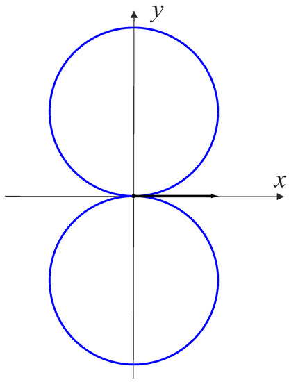
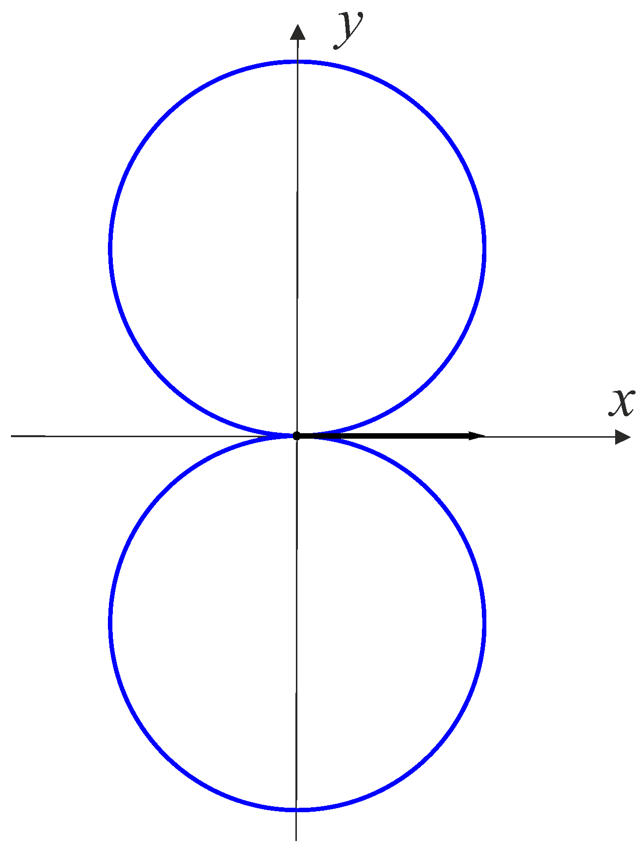
Figure 16. Extremal trajectories in $O_4^{\pm }$.

Theorem 7. 

For $h^0\in O_4^{s_2}$, the corresponding extremal trajectory is given by the circle

$$x\left(t\right)=cot\alpha sin(tsin\alpha ),y\left(t\right)=s_{2}cot\alpha (1-cos(tsin\alpha )),\theta \left(t\right)=s_{2}tsin\alpha ,t\ge 0.$$

6.6. The Domain $\mathcal{E}=1$ and $h_1=1$

When $h^0\in S_5$, i.e., $h^0=(1,0,0)$, the Hamiltonian system (17)–(19) is reduced to

$$\dot{x}=1,\dot{y}=\dot{\theta }=0,{\dot{h}}_1={\dot{h}}_2={\dot{h}}_3=0,$$

which is easily integrated

$$x\left(t\right)=t,y\left(t\right)=0,\theta \left(t\right)=0,h_1\left(t\right)=1,h_2\left(t\right)=0,h_3\left(t\right)=0.$$

Theorem 8. 

For $h^0\in S_5$, i.e., $h^0=(1,0,0)$, the corresponding extremal trajectory is the ray

$$x\left(t\right)=t,y\left(t\right)=\theta \left(t\right)=0,t\ge 0.$$

(47)

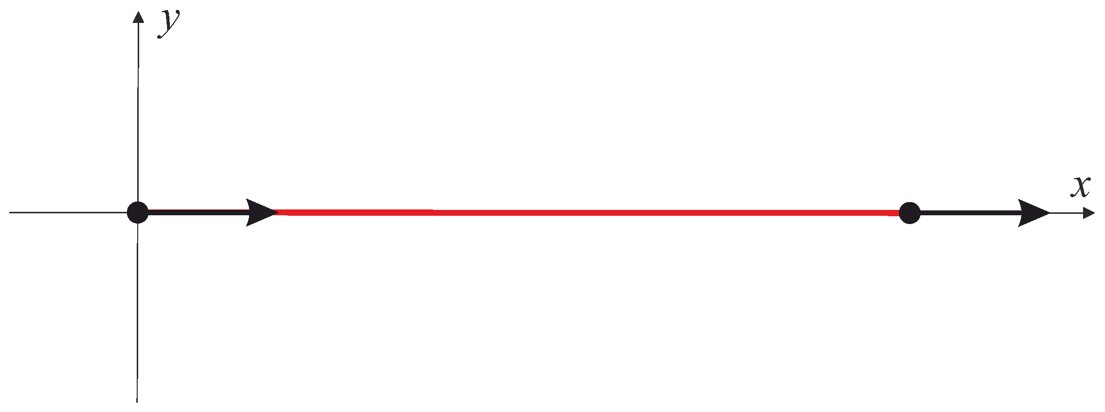
The extremal trajectory for $h^0\in S_5$ is depicted in Figure 17.

Figure 17. Extremal trajectory in $S_5$.

7. Optimality of Extremal Trajectories

7.1. General Upper Bound of Cut Time

The limitation of the Pontryagin maximum principle is that it is only a necessary but not a sufficient condition of optimality. It provides a Hamiltonian system for the extremals, which are first-order candidates for being optimal among all admissible trajectories of a control system. An extremal loses its optimality at a cut point [20].

In this section, we provide an upper bound of the cut time for a time-optimal problem

$$\begin{array}{cc}\hfill & \dot{q}=u_1{X}_1+u_2{X}_2,q=(x,y,\theta )\in {SE}_2,u=(u_1,u_2)\in U\subset {\mathbb{R}}^2,\hfill \end{array}$$

(48)

$$\begin{array}{cc}\hfill & X_1=cos\theta \frac{\partial }{\partial x}+sin\theta \frac{\partial }{\partial y},X_2=\frac{\partial }{\partial \theta },\hfill \end{array}$$

(49)

$$\begin{array}{cc}\hfill & q\left(0\right)=q_0,q\left(t_1\right)=q_1,\hfill \end{array}$$

(50)

$$\begin{array}{cc}\hfill & t_1\to min.\hfill \end{array}$$

(51)

Recall that the cut time for a trajectory $q(·)$ of an optimal control problem is defined as

$$t_{cut}\left(q(·)\right)=sup\left\{T>0\mid {\left.q\right|}_{[0,T]}\mathrm{is}\mathrm{optimal}\right\}.$$

A trajectory $q\left(t\right)=\left(x\right(t),y(t),\theta (t\left)\right)$, $t\in \mathbb{R}$, of the control system (48) is called quasiperiodic with a period $T>0$ if the following two conditions hold:

(1)

$\theta \left(t\right)=\theta (t+T)$ for all $t\in \mathbb{R}$;

(2)

There exists a linear function $l:{\mathbb{R}}^2\to \mathbb{R}$, $l\ne 0$ such that

$$l\left(x\right(t+T),y(t+T\left)\right)=l\left(x\right(t),y(t\left)\right)\mathrm{for}\mathrm{all}t\in \mathbb{R}.$$

(52)

Proposition 2. 

Let the time-optimal Problem (48)–(51) satisfies the hypotheses:

(1)

$u_1^2+u_2^2\le 1$ and $u_1>0$ for any $u=(u_1,u_2)\in U$;

(2)

$(1,0)\in U$.

Let a trajectory $q\left(t\right)=\left(x\right(t),y(t),\theta (t\left)\right)$, $t\in \mathbb{R}$, of the control system (48) be quasiperiodic with a period $T>0$. Assume moreover that the curve $\gamma \left(t\right)=\left(x\right(t),y(t\left)\right)$, $t\in \mathbb{R}$, is not a straight line.

Then, the cut time of the trajectory $q(·)$ for the time-optimal problem (48)–(51) admits an upper bound

$$t_{cut}\left(q(·)\right)\le 2T.$$

(53)

Proof. 

Consider the function l from Condition (52). The function $f\left(t\right)=l\left(x\right(t),y(t\left)\right)$ is T-periodic and continuous, thus it attains a maximum $M=f\left(\tau \right)$, $\tau \in [0,T]$. The curve $\gamma \left(t\right)$ is tangent to the straight line $l^{-1}\left(M\right)$ for each value of the parameter $t=\tau +nT$, $n\in \mathbb{Z}$. Moreover, $\gamma$ is distinct from the line $l^{-1}\left(M\right)$, thus the control $u(·)$ corresponding to the trajectory $q(·)$ satisfies the inequality $u\left(t\right)\not\equiv 1$. On the other hand, the vector ${\left.(\dot{x},\dot{y})\right|}_{\tau }={\left.u_1(cos\theta ,sin\theta )\right|}_{\tau }$ is collinear with the line $l^{-1}\left(M\right)$, as well as the vector ${\left.(cos\theta ,sin\theta )\right|}_{\tau }$.

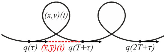
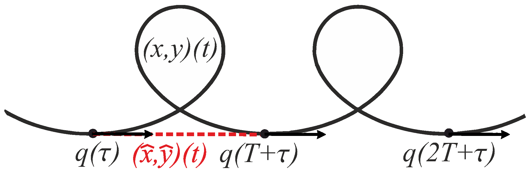
Consider now the trajectory $\widehat{q}(·)$ of the control system (48) with the initial condition $\widehat{q}\left(0\right)=q\left(\tau \right)$ and the control $u\equiv (1,0)$. There exists ${\widehat{t}}_1>0$ such that $\widehat{q}\left({\widehat{t}}_1\right)=q(\tau +T)$. Since $u\left(t\right)\not\equiv 1$, then ${\widehat{t}}_1<T$. Indeed, $(\widehat{x},\widehat{y})\left(t\right)$, $t\in [0,{\widehat{t}}_1]$, is a straight line segment connecting the points $(x,y)\left(\tau \right)$ and $(x,y)(\tau +T)$, while $(x,y)\left(t\right)$, $t\in [\tau ,\tau +T]$, is a curvilinear arc connecting the same points (see Figure 18). Thus, the trajectory ${\left.q\right|}_{[\tau ,\tau +T]}$ is not optimal for Problem (48)–(51).

Figure 18. Nonoptimal arc of the extremal trajectory.

The arc ${\left.q\right|}_{[0,2T]}$ is not optimal as well since it contains a non-optimal arc ${\left.q\right|}_{[\tau ,\tau +T]}$. The required bound (53) follows. □

Remark 8. 

It is obvious that Proposition 2 is applicable to the time-optimal Problem (2), (3) on ${SE}_2$ with control in a circular sector.

7.2. Optimality of Extremals for $cos\alpha <\mathcal{E}<1$

In this subsection, we analyze optimality of the extremal trajectories for $h^0\in S_1^{\pm }\cup O_1^{\pm }$, described in Section 6.2.

Proposition 3. 

Let $q\left(t\right)$, $t\in {\mathbb{R}}^{+}$, be an extremal trajectory in the time-optimal Problem (2), (3). Assume that the corresponding initial covector $h^0\in S_1^{\pm }\cup O_1^{\pm }$, and let $T_o$ and $T_s$ be the traveling time along full O and full S arc, given by (25) and (23).

The trajectory $q\left(t\right)$, $t\in [0,t_1]$, is not optimal if $t_1>2(T_o+T_s)$. In particular,

$$t_{cut}\left(q(·)\right)\le 2(T_o+T_s).$$

Proof. 

First, we fix the sign $h^0\in S_1^{+}\cup O_1^{+}$. The proof for $h^0\in S_1^{-}\cup O_1^{-}$ follows by Remark 5.

To prove the proposition, we rely on the general upper bound of cut time in Proposition 2, where obviously the Hypotheses (1) and (2) hold. Let us show that the extremal trajectory $q\left(t\right)$ is quasiperiodic with the period $T=T_o+T_s$. To this end, without loss of generality, we fix the initial covector $h^0=h_o^{+}=\left(cos\alpha ,sin\alpha ,\sqrt{k^2-{cos}^2\alpha }\right)$ corresponding to the beginning of the circular arc of the extremal $q\left(t\right)$. The result for another choice of initial covector follows by left-invariance (21). Denote by $h_s^{+}=\left(cos\alpha ,sin\alpha ,-\sqrt{k^2-{cos}^2\alpha }\right)$ the covector at the end of the circular arc (see Figure 7). Periodicity by $\theta$ follows by direct computation from Theorem 4:

$${\omega }^{\theta }(T_o,h_o^{+})+{\sigma }^{\theta }(T_s,h_s^{+})=2\pi ,$$

where by ${\omega }^{\theta }(t,h_o^{+})$ and ${\sigma }^{\theta }(t,h_s^{+})$, we denote the $\theta$-component of the operators $\omega (t,h_o^{+})$ and $\sigma (t,h_s^{+})$, which are the flows from Id along the O and S arcs, respectively. Thus,

$$\theta \left(T\right)-\theta \left(0\right)=2\pi \Rightarrow \theta \left(T\right)=\theta \left(0\right)\left(mod2\pi \right),\sin \mathrm{ce}\theta \in S^1=\mathbb{R}/2\pi \mathbb{Z}.$$

Now, note that the extremal control $(u_1,u_2)\left(t\right)$ is periodic with the period $T=T_o+T_s$, and thus the components $(x,y)\left(t\right)$ of the corresponding extremal trajectory satisfy

$$(x,y)\left(2T\right)-(x,y)\left(T\right)=(x,y)\left(T\right)-(x,y)\left(0\right).$$

Thus, by Proposition 2, the extremal trajectory $q\left(t\right)$ is quasiperiodic and admits the upper bound for the cut time $t_{cut}\left(q(·)\right)\le T=2(T_o+T_s)$. □

7.3. Optimality of Extremals for $\mathcal{E}>1$

In this subsection, we analyze optimality of the extremal trajectories for $h^0\in S_2^{\pm }\cup O_2^{\pm }$, described in Section 6.3.

Proposition 4. 

Let $q\left(t\right)$, $t\in {\mathbb{R}}^{+}$, be an extremal trajectory in the time-optimal Problem (2), (3). Assume that the corresponding initial covector $h^0\in S_2^{\pm }\cup O_2^{\pm }$, and let $T_o$ and $T_s$ be the traveling time along full O and full S arc, given by (33) and (31).

The trajectory $q\left(t\right)$, $t\in [0,t_1]$, is not optimal if $t_1>4(T_o+T_s)$. In particular,

$$t_{cut}\left(q(·)\right)\le 4(T_o+T_s).$$

Proof. 

The proof is similar to the proof of Proposition 4. The only difference appears in the periodicity by $\theta$. In the case $h^0\in S_2^{\pm }\cup O_2^{\pm }$, we have $\theta \left(T\right)-\theta \left(0\right)=0$, $T=2(T_o+T_s)$, which follows from Theorem 5. □

7.4. Optimality of Separatrix Extremals ($\mathcal{E}=1$, $h_{10}\ne 1$)

In this subsection, we analyze optimality of extremal trajectories for $h^0\in S_3\cup O_3$, described in Section 6.4.

Proposition 5. 

Let $q\left(t\right)$, $t\in {\mathbb{R}}^{+}$, be an extremal trajectory in Problem (2), (3). Assume that the initial covector $h^0\in S_3\cup O_3$. The trajectory $q\left(t\right)$ is optimal for $t\in [0,t_{01}]$, i.e, it is optimal before the first switching. In particular, for $h^0\in S_3^{\pm \mp }$, the trajectory $q\left(t\right)$ is optimal up to infinity.

Proof. 

The extremal trajectory $q\left(t\right)$ is given by Theorem 6. For $h^0\in O_2^{\pm }$, the corresponding trajectory $q\left(t\right)$, $t\in [0,t_{01}]$ is given by an arc of circular extremal, which is optimal as we prove in Proposition 6. For $h^0\in S_3$, the corresponding extremal trajectory before the first switching is given by an arc of separatrix sub-Riemannian geodesic in ${SE}_2$, which is optimal, as proved in [4]. In particular, for $h^0\in S_3^{\pm \mp }$, the trajectory $q\left(t\right)$ is optimal up to infinity since it has no switchings. □

Remark 9. 

An upper bound of the cut time for the separatrix extremals of general type, which have the switching points, remains an open problem.

7.5. Optimality of Circular Trajectories, $\mathcal{E}\le$ cos $\alpha$

In this subsection, we analyze optimality of circular extremals described in Section 6.5.

Proposition 6. 

Let $q\left(t\right)$, $t\in \mathbb{R}$, be an extremal trajectory in the time-optimal Problem (2), (3). Assume that $q(·)$ is of circular type and let $T_o=\frac{2\pi }{sin\alpha }$ be its period.

A trajectory $q\left(t\right)$, $t\in [0,t_1]$, is optimal iff $t_1\in [0,T_o)$. In particular,

$$t_{cut}\left(q(·)\right)=T_o.$$

Moreover, for any $t_1\in [0,T_o)$, the trajectory $q\left(t\right)$, $t\in [0,t_1]$, is a unique optimal trajectory connecting $q_0$ to $q\left(t_1\right)$.

Proof. 

First of all, a full circular arc $q\left(t\right)$, $t\in [0,T_o]$, is not optimal since it connects the same points $q\left(0\right)=q\left(T_o\right)$ in a positive time $T_o$.

Now we prove that for any $t_1\in (0,T_o)$, the trajectory $q\left(t\right)$, $t\in [0,t_1]$, is a unique optimal trajectory connecting $q_0$ to $q\left(t_1\right)$. By contradiction, suppose that there is another trajectory $\tilde{q}\left(t\right)=(\tilde{\theta },\tilde{x},\tilde{y})\left(t\right)$, $t\in [0,{\tilde{t}}_1]$, with a control $({\tilde{u}}_1,{\tilde{u}}_2)\left(t\right)$ such that ${\tilde{t}}_1\le t_1$ and $\tilde{q}\left(0\right)=q_0$, $\tilde{q}\left({\tilde{t}}_1\right)=q\left(t_1\right)$. We have $\dot{\tilde{\theta }}\left(t\right)={\tilde{u}}_2\left(t\right)\le sin\alpha$, moreover, this inequality becomes strict on a nonempty interval since the trajectory $\tilde{q}(·)$ is not circular. Thus,

$$t_{1}sin\alpha =\theta \left(t_1\right)=\tilde{\theta }\left({\tilde{t}}_1\right)={\int }_0^{{\tilde{t}}_1}{\tilde{u}}_2\left(t\right)dt<{\tilde{t}}_{1}sin\alpha \le t_{1}sin\alpha ,$$

whence $t_{1}sin\alpha <t_{1}sin\alpha$, a contradiction. □

7.6. Optimality of the Straight Trajectory ($\mathcal{E}=1$, $h_{10}=1$)

In this subsection, we analyze the optimality of the straight extremal (47) (see Section 6.6).

Proposition 7. 

The straight extremal trajectory (47) in Problem (2), (3) is optimal up to infinity.

Proof. 

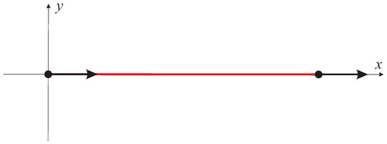
Since $u_1\le 1$, an end point $(t,0,0)$ cannot be reached from Id by time $<t$. □

7.7. Lower Bound of Cut Time

Proposition 8. 

Let $q\left(t\right)$, $t\in [0,t_1]$, be an extremal trajectory in the time-optimal problem on ${SE}_2$ with control in a circular sector. Assume that $q(·)$ is of sub-Riemannian type.

If $q(·)$ is optimal for the sub-Riemannian problem on ${SE}_2$, then it is optimal in the time-optimal problem on ${SE}_2$ with control in a circular sector. Thus,

$$t_{cut}\left(q(·)\right)\ge t_{cut}^{SR}\left(q(·)\right),$$

where$t_{cut}^{SR}\left(q(·)\right)$ is the cut time of the trajectory $q(·)$ for the sub-Riemannian problem on ${SE}_2$ (see [4]).

In particular, there exists $\epsilon >0$ such that $t_{cut}\left(q(·)\right)>\epsilon$.

Proof. 

The sub-Riemannian problem on ${SE}_2$ can be stated as a time-optimal problem with a set of control parameters given by the full disc. Now the statements of this proposition are obvious since if a trajectory is optimal for a problem with a bigger set of control parameters, then it is also optimal for a problem with a smaller set of control parameters. □

Now, Propositions 6 and 8 imply the following.

Corollary 1. 

Let $q\left(t\right)$, $t\in [0,t_1]$, be an extremal trajectory in the time-optimal problem on ${SE}_2$ with control in a circular sector. Then, there exists $\epsilon >0$ such that $t_{cut}\left(q(·)\right)>\epsilon$.

8. Conclusions

We considered the time minimization Problem (2), (3) in the roto-translation group ${SE}_2$ with admissible control in a circular sector. The problem reveals the trajectories of a car model that can move forward on a plane and turn with a given minimum turning radius. The model generalizes the sub-Riemannian length minimizers problem by adding a restriction on the velocity vector to lie in a circular sector with the opening angle $2\alpha \in S^1$.

We studied the local and global controllability of the system and the existence of the solution for given arbitrary boundary conditions in Theorem 1. We obtained the following.

1.

For $\alpha =0$, the system is not globally controllable.

2.

For $\alpha \in (0,\frac{\pi }{2}]$, the system is globally but not small-time locally controllable.

3.

For $\alpha \in (\frac{\pi }{2},\pi )$, the problem is ill-posed. The system is globally and small-time locally controllable, but an optimal trajectory does not exist for some boundary conditions.

4.

For $\alpha =\pi$, the system is globally and small-time locally controllable. This case coincides with the sub-Riemannian length minimizers problem in ${SE}_2$.

Then, we considered the well-posed case $\alpha \in (0,\frac{\pi }{2}]$.

We obtained a lower bound for local controllability time $T=\frac{2\pi }{sin\alpha }$ (see Theorem 2).

We applied PMP and obtained explicit expressions for the extremals.

We showed that arclength parameterized abnormal extremals are given by joining of the half period arcs of the circular extremals (see Theorem 3).

We showed that there are five qualitative types of normal extremal trajectories.

1.

Arcs of noninflectional sub-Riemannian geodesics in ${SE}_2$, joined by arcs of circular extremals. The exact expression is given by Theorem 4. An upper bound for the cut time is given by Proposition 3.

2.

Arcs of inflectional sub-Riemannian geodesics in ${SE}_2$, joined by arcs of circular extremals. The exact expression is given by Theorem 5. An upper bound for the cut time is given by Proposition 4.

3.

Arcs of the separatrix sub-Riemannian geodesics in ${SE}_2$ joined by an arc of the circular extremal. The exact expression is given by Theorem 6. The extremals before the first switching are optimal (see Proposition 5).

4.

The circular extremals. The exact expression is given by Theorem 7. The cut time is given by Proposition 6.

5.

The straight extremal. The exact expression is given by Theorem 8. It is optimal up to infinity (see Proposition 7).

We showed that small arcs of the normal extremals are optimal (see Corollary 1).

As a further extension of the present work, we plan to use the obtained exact expressions for the extremals and the bounds for the cut time to construct the optimal synthesis; similarly, it is performed for the sub-Riemannian length minimizer problem in ${SE}_2$ [4].

References

- Dubins, L.E. On Curves of Minimal Length with a Constraint on Average Curvature, and with Prescribed Initial and Terminal Positions and Tangents. Am. J. Math. 1975, 79, 497–516. [Google Scholar] [CrossRef] [Scilit]
- Reeds, J.A.; Shepp, L.A. Optimal paths for a car that goes both forwards and backwards. Pac. J. Math. 1990, 145, 367–393. [Google Scholar] [CrossRef] [Scilit]
- Ardentov, A.A. Markov–Dubins problem with Control on a Triangle. In Proceedings of the International Voronezh Spring Mathematical School Dedicated to the 115th Anniversary of the Birth of Academician L.S. Pontryagin, Voronezh, Russia, 3–9 May 2023; pp. 43–44. (In Russian) [Google Scholar]
- Sachkov, Y.L. Cut locus and optimal synthesis in the sub-Riemannian problem on the group of motions of a plane. ESAIM: Control. Optim. Calc. Var. 2011, 17, 293–321. [Google Scholar] [CrossRef] [Scilit]
- Berestovskii, V.N. Geodesics of a left-invariant nonholonomic Riemannian metric on the group of motions of the Euclidean plane. Sib. Math. J. 1994, 35, 1083–1088. [Google Scholar] [CrossRef] [Scilit]
- Duits, R.; Meesters, S.P.L.; Mirebeau, J.-M.; Portegies, J.M. Optimal Paths for Variants of the 2D and 3D Reeds–Shepp Car with Applications in Image Analysis. J. Math. Imaging Vis. 2018, 60, 816–848. [Google Scholar] [CrossRef] [Scilit]
- Mashtakov, A.P. Time minimization problem on the group of motions of a plane with admissible control in a half-disk. Mat. Sb. 2022, 213, 100–122. (In Russian) [Google Scholar]
- Lynch, K.M.; Park, F.C. Modern Robotics. Mechanics, Planning, and Control; Cambridge University Press: Cambridge, UK, 2017. [Google Scholar]
- Arismendi, C.; Alvarez, D.; Garrido, S.; Moreno, L. Nonholonomic Motion Planning Using the Fast Marching Square Method. Int. J. Adv. Robot. Syst. 2015, 12, 60129. [Google Scholar] [CrossRef] [Scilit]
- Boscain, U.V.; Chitour, Y. Time-Optimal Synthesis for Left-Invariant Control Systems on SO(3). SIAM J. Control Optim. 2005, 44, 111–139. [Google Scholar] [CrossRef] [Scilit]
- Hubel, D.H.; Wiesel, T.N. Receptive fields of single neurones in the cat’s striate cortex. J. Physiol. 1959, 148, 574. [Google Scholar] [CrossRef] [Scilit]
- Petitot, J. The neurogeometry of pinwheels as a sub-Riemannian contact structure. J. Physiol. 2003, 97, 265–309. [Google Scholar] [CrossRef] [Scilit]
- Citti, G.; Sarti, A. A cortical based model of perceptual completion in the roto-translation space. J. Math. Imaging Vis. 2006, 24, 307–326. [Google Scholar] [CrossRef] [Scilit]
- Duits, R.; Boscain, U.; Rossi, F.; Sachkov, Y.L. Association Fields via Cuspless Sub-Riemannian Geodesics in SE(2). J. Math. Imaging Vis. 2014, 49, 384–417. [Google Scholar] [CrossRef] [Scilit] [PubMed]
- Franceschiello, B.; Mashtakov, A.; Citti, G.; Sarti, A. Geometrical optical illusion via sub-Riemannian geodesics in the roto-translation group. Differ. Geom. Appl. 2019, 65, 55–77. [Google Scholar] [CrossRef] [Scilit]
- Baspinar, E.; Calatroni, L.; Franceschi, V.; Prandi, D. A Cortical-Inspired Sub-Riemannian Model for Poggendorff-Type Visual Illusions. J. Imaging 2021, 7, 41. [Google Scholar] [CrossRef] [Scilit] [PubMed]
- Boscain, U.; Gauthier, J.; Prandi, D.; Remizov, A. Image reconstruction via non-isotropic diffusion in Dubins/Reed-Shepp-like control systems. In Proceedings of the 53rd IEEE Conference on Decision and Control, Los Angeles, CA, USA, 15–17 December 2014; pp. 4278–4283. [Google Scholar]
- Bekkers, E.J.; Duits, R.; Mashtakov, A.; Sanguinetti, G.R. A PDE Approach to Data-driven Sub-Riemannian Geodesics in SE(2). Siam J. Imaging Sci. 2015, 8, 2740–2770. [Google Scholar] [CrossRef] [Scilit]
- Chen, D.; Mirebeau, J.-M.; Shu, M.; Cohen, L.D. Computing geodesic paths encoding a curvature prior for curvilinear structure tracking. Proc. Natl. Acad. Sci. USA 2023, 120, e2218869120. [Google Scholar] [CrossRef] [Scilit]
- Agrachev, A.A.; Sachkov, Y.L. Control Theory from the Geometric Viewpoint; Springer: Berlin/Heidelberg, Germany, 2004. [Google Scholar]
- Jurdjevic, V. Rolling Geodesics, Mechanical Systems and Elastic Curves. Mathematics 2022, 10, 4827. [Google Scholar] [CrossRef] [Scilit]
- Jurdjevic, V. Integrable Systems: In the Footprints of the Greats. Mathematics 2023, 11, 1063. [Google Scholar] [CrossRef] [Scilit]
- Mashtakov, A.P.; Sachkov, Y.L. Extremal Trajectories in a Time Minimization Problem on the Group of Motions of a Plane with Admissible Control in a Circular Sector. Tr. Mat. Instituta Im. V.A. Steklova 2023, 321, 215–222. [Google Scholar]
- Bonnard, B.; Jurdjevic, V.; Kupka, I.; Sallet, G. Transitivity of families of invariant vector fields on the semidirect products of Lie groups. Trans. Am. Math. Soc. 1982, 271, 525–535. [Google Scholar] [CrossRef]
- Agrachev, A.; Barilari, D.; Boscain, U. A Comprehensive Introduction to Sub-Riemannian Geometry; Cambridge Studies in Advanced Mathematics; Cambridge University Press: Cambridge, UK, 2019. [Google Scholar]
- Lokutsievskiy, L.V. Convex trigonometry with applications to sub-Finsler geometry. Sb. Math. 2019, 210, 1179–1205. [Google Scholar] [CrossRef] [Scilit]
- Arnold, V.I. Ordinary Differential Equations; Springer: Berlin/Heidelberg, Germany, 1992. [Google Scholar]
- Sachkov, Y.L. Left-invariant optimal control problems on Lie groups that are integrable by elliptic functions. Uspekhi Mat. Nauk. 2023, 78, 67–166. [Google Scholar] [CrossRef] [Scilit]
Disclaimer/Publisher’s Note: The statements, opinions and data contained in all publications are solely those of the individual author(s) and contributor(s) and not of MDPI and/or the editor(s). MDPI and/or the editor(s) disclaim responsibility for any injury to people or property resulting from any ideas, methods, instructions or products referred to in the content. |
© 2023 by the authors. Licensee MDPI, Basel, Switzerland. This article is an open access article distributed under the terms and conditions of the Creative Commons Attribution (CC BY) license (https://creativecommons.org/licenses/by/4.0/).