Stochastic Strike-Slip Fault as Earthquake Source Model

Abstract

It is known that the source of a tectonic earthquake in the framework of the theory of elasticity and viscoelasticity is considered to be displacement along a certain fault surface. Usually, when describing a source, the geometry of the fault surface is simplified to a flat rectangular area. The displacement vector is assumed to be constant. In this paper, we propose a model of an earthquake source in the form of a displacement with a constant vector along a stochastic uneven surface. A number of standard assumptions are made during the modeling. We take into account only the elastic properties of the medium. We consider the Earth’s crust as a half-space and assume that the medium is homogeneous and isotropic. For the mathematical description of the earthquake source, we use the classical force equivalent of displacement along the fault. This is the distribution of double pairs of forces. The field of displacements under the action of body forces is found through a combination of Mindlin nuclei of strain. The paper presents numerical analytic solutions for displacement along the strike-slip fault corresponding to one of an earthquake source mechanism. We propose to introduce a random deformation of a rectangular flat fault surface. The paper shows the results of a computational experiment comparing the levels and regions of relative deformations of the Earth’s crust in the case of displacement along a flat fault surface and along a stochastic uneven one. In the case of a stochastic fault surface, the regions of relative deformations become asymmetric. Such differences from the classical case can be useful for an explanation as to why in some cases the simulation results differ from the results of observations.

1. Introduction

The source of a tectonic earthquake occurs as a result of the complete or partial relaxation of stress accumulated by the Earth’s material during tectonic deformation. At this time, there is a local loss of stability of the medium; its continuity is violated [1,2]. As a result, the accumulated elastic strain energy transforms into an inelastic one. In the framework of the theory of elasticity and viscoelasticity, the earthquake source is considered a dislocation, i.e., displacement along a certain fault surface [3]. In addition to the geometry of this surface, the earthquake source is characterized by its orientation and position in space, as well as by the field of the slip vector along the rupture surface. When describing the source, the following assumptions are most often used: the surface geometry is simplified to a flat rectangular area [4,5,6], and the displacement vector is assumed to be constant [7,8]. Such simplifications make it possible to obtain analytical solutions to the problem of determining the displacement field of the Earth’s crust at the time of an earthquake [9].

The Earth’s crust consists of separate layers of rocks. They have various mechanical properties. The direct consideration of these properties when constructing models of mechanical processes occurring in rocks is difficult. It is possible to indirectly take into account the mechanical properties of rocks by introducing stochastic components. Thus, the problem of the probabilistic characteristics of the displacement vector in the earthquake source was previously investigated [10]. It was shown that the probability distribution of the normalized displacement value has stability. It is similar to the exponential one, but has a heavy tail. In addition, a compact description of the distribution was proposed using the lognormal law with a negative shift of the density function and winsorization at zero. The described approach, as well as similar ones, were used in modeling displacements of the Earth’s surface to calculate the strength of engineering structures [11,12,13]. Also, the effect of adding a slip deficit to the stochastic fault model on the slip distribution in the subduction zone was considered [14]. An overview of the methods for adding stochastic components into the earthquake source model is presented in Gusev’s paper [15].

The geometric shape of the fault surface is one of the main characteristics of the earthquake source. Usually, when modeling a source, the fault surface is considered a plane bounded by a rectangular region or as a composition of such regions [16,17,18]. In this paper, we propose a modified dislocation model of an earthquake source in the form of displacement along a stochastic surface. By the term ”stochastic surface”, we understand it to be an uneven fault surface formed by the random deformation of the plane fault surface. We obtain new numerical analytic solutions for the displacement along the stochastic strike-slip fault.

The structure of the main part of the paper is as follows. Section 2 is devoted to the mathematical formulation of the problem of the stress–strain state of the Earth’s crust in the elastic half-space approximation based on Navier equations. Earthquake source modeling based on systems of equivalent forces is carried out. Solutions are derived for determining the deformations of an elastic half-space under the action of a dislocation along an arbitrary smooth surface. A method for constructing a stochastic displacement surface in an earthquake source is described. Section 3 contains the results of the numerical modeling of the Earth’s crust deformations. The main findings and conclusion are contained in Section 4. Appendix A contains a list of the main symbols, including their physical dimensions, while Appendix B contains values for verification computational experiments.

2. Mathematical Formulation

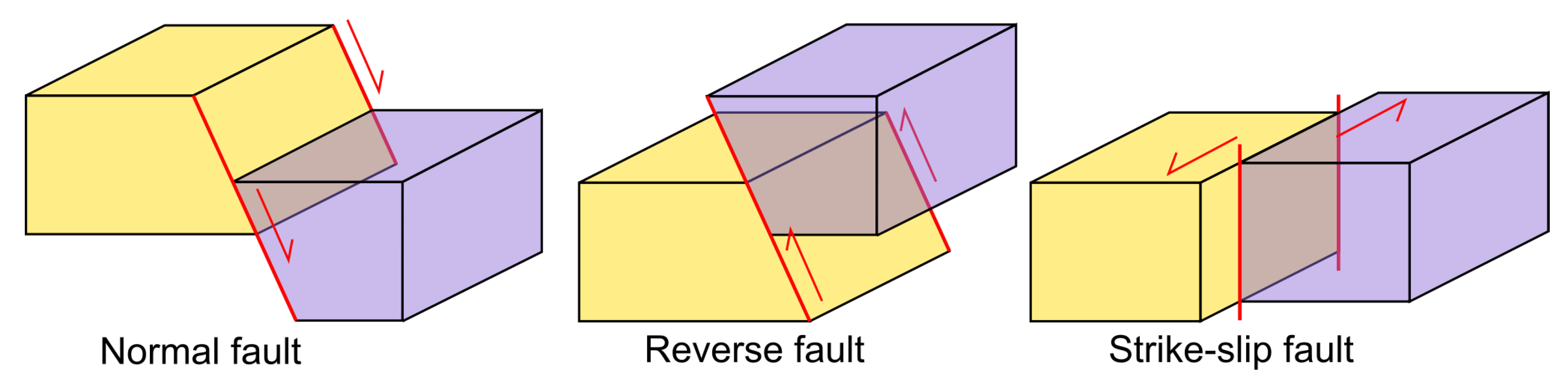
2.1. Earthquake Fault Model

According to modern concepts, a tectonic earthquake source occurs as a result of sliding along the inner surface—the fault plane [19]. There are three types of faults: normal, reverse and strike-slip (Figure 1). Strike-slip faults are associated with dominantly horizontal displacement, and normal and reverse faults with vertical displacement.

Mathematically, earthquake sources are described by a body force within the excitation area, a displacement jump on the fault surface, or deformation. Note that displacement along the fault excites the same seismic waves as some system of forces distributed over the fault with zero total moment. In general, the distribution of forces can have a different form, but in the case of an isotropic medium, it can always be chosen as the surface distribution of double pairs of forces. The classical force equivalent of displacement along a fault is the distribution of double pairs of forces. In this work, we will limit to the derivation of a solution for strike-slip earthquake.

2.2. Stress–Strain State of the Earth’s Crust

We make a number of standard assumptions during the modeling [1]. We will take into account only the elastic properties of the medium, we simplify the geometry of the Earth’s crust to a half-space, and we assume that the medium is homogeneous and isotropic. To describe such a model in a Cartesian coordinate system $(x_1,x_2,x_3)$, let us use Navier equations [20]:

$$\mu \frac{{\partial }^2{u}_i}{\partial x_j^2}+(\lambda +\mu )\frac{{\partial }^2{u}_i}{\partial x_i\partial x_j}+X_i=0,i,j=1..3,$$

(1)

where $u_i$ are the displacement vector components, $X_i$ are body forces, $\lambda ,\mu$ are Lame coefficients.

The boundary conditions of problem (1) are defined on the surface $x_3=0$ and consist in the equality of the following components of the stress tensor to zero:

$${\sigma }_{31}{|}_{x_3=0}={\sigma }_{32}{{|}_{x_3=0}={\sigma }_{33}|}_{x_3=0}=0.$$

(2)

2.3. Point Source: Mindlin Solutions

Mindlin [21,22] was engaged in solving the problem of determining the displacement field under the action of body forces located inside an elastic half-space and applied to one point. In his works, he solved this problem for differently directed single and double forces, including double forces with moments. Mindlin expressed his solutions in terms of combinations of strain nuclei for elastic space proposed by Kelvin. Mindlin solutions can also be called strain nuclei for an elastic half-space by analogy with Kelvin solutions. Solutions of differential equations system (1) with boundary conditions (2) can be expressed through these nuclei. Mindlin expressed the solutions in terms of the Galerkin vector. In the present work, equivalent solutions are constructed in the form of displacement vector components.

We take a Cartesian coordinate system. Let $u_i^j$ be the i-th component of the displacement vector at point $(x_1,x_2,x_3)$, corresponding to the single force of magnitude F at point $({\xi }_1,{\xi }_2,{\xi }_3)$ in direction j. According to Mindlin’s works, $u_i^j$ can be represented as follows:

$$\begin{array}{cc}\hfill {\displaystyle u_i^j(x_1,x_2,x_3)=}& u_{iA}^j(x_1,x_2,-x_3)-u_{iA}^j(x_1,x_2,x_3)+\hfill \\ \hfill & {\displaystyle +u_{iB}^j(x_1,x_2,x_3)+x_3{u}_{iC}^j(x_1,x_2,x_3)}\hfill \end{array}$$

(3)

$$\begin{array}{cc}\hfill & \left\{\begin{array}{c}{\displaystyle u_{iA}^j=\frac{F}{8\pi \mu }\left[(2-\alpha )\frac{{\delta }_{ij}}{R}+\alpha \frac{R_i{R}_j}{R^3}\right]}\hfill \\ {\displaystyle u_{iB}^j=\frac{F}{4\pi \mu }[\frac{{\delta }_{ij}}{R}+\frac{R_i{R}_j}{R^3}+\frac{1-\alpha }{\alpha }(\frac{{\delta }_{ij}}{R+R_3}+\frac{R_i{\delta }_{j3}-R_j{\delta }_{i3}(1-{\delta }_{j3})}{R(R+R_3)}-}\hfill \\ {\displaystyle -\frac{R_i{R}_j}{R{(R+R_3)}^2}(1-{\delta }_{i3})(1-{\delta }_{j3})\left)\right]}\hfill \\ {\displaystyle u_{iC}=\frac{F}{4\pi \mu }(1-2{\delta }_{i3})\left[(2-\alpha )\frac{R_i{\delta }_{j3}-R_j{\delta }_{i3}}{R^3}+\alpha {\xi }_3\left(\frac{{\delta }_{ij}}{R^3}-\frac{3R_i{R}_j}{R^5}\right)\right],}\hfill \end{array}\right.\hfill \end{array}$$

(4)

where $\alpha =(\lambda +\mu )/(\lambda +2\mu )$, ${\delta }_{ij}$ is Kronecker delta, $R_1=x_1-{\xi }_1$, $R_2=x_2-{\xi }_2$, $R_3=-x_3-{\xi }_3$, $R^2=R_1^2+R_2^2+R_3^2$.

To obtain solutions in the form of strain nuclei, we take the corresponding partial ${\xi }_k$ derivatives of $u_i^j(x_1,x_2,x_3)$:

$$\begin{array}{c}\hfill \frac{\partial u_i^j(x_1,x_2,x_3)}{\partial {\xi }_k}=\frac{\partial u_{iA}^j(x_1,x_2,-x_3)}{\partial {\xi }_k}-\frac{\partial u_{iA}^j(x_1,x_2,x_3)}{\partial {\xi }_k}+\\ \hfill +\frac{u_{iB}^j(x_1,x_2,x_3)}{\partial {\xi }_k}+x_3\frac{\partial u_{iC}^j(x_1,x_2,x_3)}{\partial {\xi }_k}\end{array}$$

(5)

$$\begin{array}{c}\hfill \left\{\begin{array}{c}{\displaystyle \frac{\partial u_{iA}^j}{\partial {\xi }_k}=\frac{F}{8\pi \mu }\left\{(2-\alpha )\frac{R_k}{R^3}{\delta }_{ij}-\alpha \frac{R_i{\delta }_{jk}+R_j{\delta }_{ik}}{R^3}+3\alpha \frac{R_i{R}_j{R}_k}{R^5}\right\}}\hfill \\ {\displaystyle \frac{\partial u_{iB}^j}{\partial {\xi }_k}=\frac{F}{4\pi \mu }\{-\frac{R_i{\delta }_{jk}+R_j{\delta }_{ik}-R_k{\delta }_{ij}}{R^3}+\frac{3R_i{R}_j{R}_k}{R^5}+}\hfill \\ {\displaystyle +\frac{1-\alpha }{\alpha }[\frac{{\delta }_{3k}R+R_k}{R{(R+R_3)}^2}{\delta }_{ij}-\frac{{\delta }_{ik}{\delta }_{j3}-{\delta }_{jk}{\delta }_{i3}(1-{\delta }_{j3})}{R(R+R_3)}+}\hfill \\ {\displaystyle +[R_i{\delta }_{j3}-R_j{\delta }_{i3}(1-{\delta }_{j3})]\frac{{\delta }_{3k}{R}^2+R_k(2R+R_3)}{R^3{(R+R_3)}^2}+[\frac{R_i{\delta }_{jk}+R_j{\delta }_{ik}}{R{(R+R_3)}^2}-}\hfill \\ {\displaystyle -R_i{R}_j\frac{2{\delta }_{3k}{R}^2+R_k(3R+R_3)}{R^3{(R+R_3)}^3}\left](1-{\delta }_{i3})(1-{\delta }_{j3})\right]\}}\hfill \\ {\displaystyle \frac{\partial u_{iC}^j}{\partial {\xi }_k}=\frac{F}{4\pi \mu }(1-2{\delta }_{i3})\left\{(2-\alpha )\right[\frac{{\delta }_{jk}{\delta }_{i3}-{\delta }_{ik}{\delta }_{j3}}{R^3}+}\hfill \\ {\displaystyle +\frac{3R_k(R_i{\delta }_{j3}-R_j{\delta }_{i3})}{R^5}]+\alpha \left[\frac{{\delta }_{ij}}{R^3}-\frac{3R_i{R}_j}{R^5}\right]{\delta }_{3k}+}\hfill \\ {\displaystyle +3\alpha {\xi }_3\left[\frac{R_i{\delta }_{jk}+R_j{\delta }_{ik}+R_k{\delta }_{ij}}{R^5}-\frac{5R_i{R}_j{R}_k}{R^7}\right]\}}\hfill \end{array}\right.\end{array}$$

(6)

2.4. Distributed Source

Using the Volterra dislocation principle, Steketee showed [3] that the displacement field caused by movement along the fault plane $\Sigma$ in an elastic half-space can be found through a surface integral of the following form:

$$u_i=\frac{1}{F}\underset{\Sigma }{\int \int }\Delta u_j[\lambda {\delta }_{kj}\frac{\partial u_i^n}{\partial {\xi }_n}+\mu (\frac{\partial u_i^k}{\partial {\xi }_j}+\frac{\partial u_i^j}{\partial {\xi }_k}\left)\right]n_{j}d\Sigma ,$$

(7)

where $\Delta u_j$ is a dislocation in the j-th direction across the fault surface $\Sigma$, and $n_j$ is the direction cosines of the normal to the surface element $d\Sigma$. If $k=j$, then $\partial u_i^k/\partial {\xi }_j$ are strain nuclei corresponding to double forces without moment (Figure 2a), and $\partial u_i^n/\partial {\xi }_n$ is the strain nuclei combination corresponding to the dilation center. If $k\ne j$, then $(\partial u_i^k/\partial {\xi }_j+\partial u_i^j/\partial {\xi }_k)$ are strain nuclei corresponding to two perpendicular pairs of double forces with moments (Figure 2b). Figure 2 shows the systems of forces corresponding to strain nuclei combinations $\partial {\mathbf{u}}^k/\partial {\xi }_j+\partial {\mathbf{u}}^j/\partial {\xi }_k$.

In this paper, we consider earthquake source of strike-slip type. The strain nuclei combination for such an earthquake source is as follows:

$$\begin{array}{c}\hfill u_i=\frac{1}{F}\underset{\Sigma }{\int \int }\Delta u_1\lambda \left(\frac{\partial u_i^2}{\partial {\xi }_2}+\frac{\partial u_i^3}{\partial {\xi }_3}\right)+(\lambda +2\mu )\frac{\partial u_1^n}{\partial {\xi }_1}]n_1+\\ \hfill +\left[\mu \left(\frac{\partial u_i^1}{\partial {\xi }_2}+\frac{\partial u_i^2}{\partial {\xi }_1}\right)\right]n_2+\left[\mu \left(\frac{\partial u_i^1}{\partial {\xi }_3}+\frac{\partial u_i^3}{\partial {\xi }_1}\right)\right]n_3\}d\Sigma .\end{array}$$

(8)

Let the fault surface $\Sigma$ be explicitly given by the equation ${\xi }_2=f({\xi }_1,{\xi }_3)$. In this case, the unit normal $\mathbf{n}$ at each point $\xi ({\xi }_1,{\xi }_2,{\xi }_3)$ of the surface can be found as follows:

$$\mathbf{n}({\xi }_1,{\xi }_2,{\xi }_3)=\frac{\left({\displaystyle \frac{df}{d{\xi }_1}},-1,{\displaystyle \frac{df}{d{\xi }_3}}\right)}{\sqrt{{\left({\displaystyle \frac{df}{d{\xi }_1}}\right)}^2+1+{\left({\displaystyle \frac{df}{d{\xi }_3}}\right)}^2}}.$$

(9)

We denote integrand (8) by ${\mathsf{\Omega }}_{strike}({\xi }_1,{\xi }_2,{\xi }_3)$:

$$\begin{array}{c}\hfill {\mathsf{\Omega }}_{strike}^i({\xi }_1,{\xi }_2,{\xi }_3)=\Delta u_1\left\{\right[\lambda (\frac{\partial u_i^2}{\partial {\xi }_2}+\frac{\partial u_i^3}{\partial {\xi }_3})+(\lambda +2\mu )\frac{\partial u_1^n}{\partial {\xi }_1}]n_1+\\ \hfill +\left[\mu \left(\frac{\partial u_i^1}{\partial {\xi }_2}+\frac{\partial u_i^2}{\partial {\xi }_1}\right)\right]n_2+\left[\mu \left(\frac{\partial u_i^1}{\partial {\xi }_3}+\frac{\partial u_i^3}{\partial {\xi }_1}\right)\right]n_3\}\end{array}$$

(10)

We place the fault surface $\Sigma$ at the depth $C<0$. The projection $D_{x_1{x}_3}$ of this surface onto the plane $x_2=0$ is a rectangular area (Figure 3).

Let us perform parametrization and move from the surface integral to a double, and then to an iterated one:

$$u_i=\frac{1}{F}\underset{-L/2}{\overset{L/2}{\int }}d{\xi }_1\underset{C-W/2}{\overset{C+W/2}{\int }}{\mathsf{\Omega }}_{slip}^i({\xi }_1,f({\xi }_1,{\xi }_3),{\xi }_3)\sqrt{{\left(\frac{df}{d{\xi }_1}\right)}^2+1+{\left(\frac{df}{d{\xi }_3}\right)}^2}d{\xi }_3.$$

(11)

Expression (11) allows us to calculate the components of the displacement field vector. The field arises as a result of displacement along the fault surface inside the elastic half-space in the strike direction.

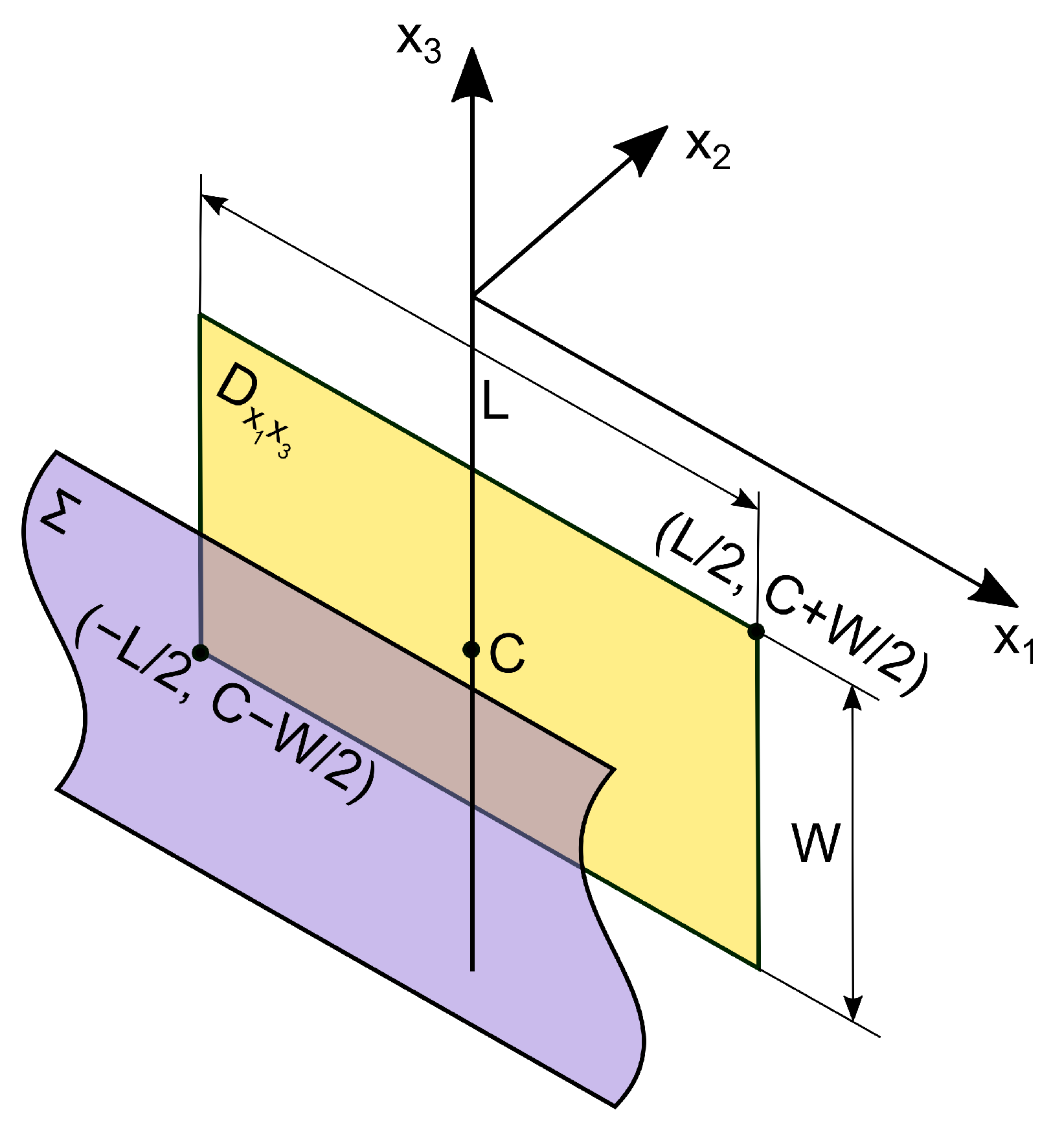
2.5. Dislocation with a Constant Displacement Vector along a Finite Rectangular Surface

We represent the displacement surface $\Sigma$ as a plane bounded by a rectangular region with dip angle $\delta$. In this case, the unit normal is $\mathbf{n}=(0,-sin(\delta ),cos(\delta \left)\right)$. The displacement vector $\Delta \mathbf{u}$ is assumed to be constant. Its components in the case of displacement along the strike are equal to $\Delta \mathbf{u}=(U,0,0)$, and in the case of displacement, along the dip $\Delta \mathbf{u}=(0,Ucos(\delta ),Usin(\delta \left)\right)$.

In this case, integral (8) will take the form

$$\begin{array}{c}\hfill u_i=\frac{\mu U}{F}\underset{\Sigma }{\int \int }\left[-\left(\frac{\partial u_i^1}{\partial {\xi }_2}+\frac{\partial u_i^2}{\partial {\xi }_1}\right)sin\left(\delta \right)+\left(\frac{\partial u_i^1}{\partial {\xi }_3}+\frac{\partial u_i^3}{\partial {\xi }_1}\right)cos\left(\delta \right)\right]d\Sigma .\end{array}$$

(12)

Given that the surface $\Sigma$ is defined by the relation ${\xi }_2=({\xi }_3-C)·\mathrm{ctg}\left(\delta \right)$, the surface integral will look like this:

$$\begin{array}{c}\hfill u_i=\frac{1}{sin\left(\delta \right)F}\underset{-L/2}{\overset{L/2}{\int }}d{\xi }_1\underset{C-\frac{Wsin\left(\delta \right)}{2}}{\overset{C+\frac{Wsin\left(\delta \right)}{2}}{\int }}{\mathsf{\Omega }}_{slip}^i({\xi }_1,({\xi }_3-C)·\mathrm{ctg}\left(\delta \right),{\xi }_3)d{\xi }_3.\end{array}$$

(13)

2.6. Stochastic Geometry of the Fault Surface

To obtain a stochastic fault surface $\Sigma$, we propose to introduce a random deformation of a rectangular flat surface $\mathsf{\Theta }$. To do that we do the following:

• We build a two-dimensional grid on the plane $\mathsf{\Theta }$ with horizontal and vertical steps $h_1$ and $h_2$, respectively (Figure 4a).
• We define a random function $\eta =\eta ({\xi }_1,{\xi }_3)$. For simplicity, we assume that $\eta ({\xi }_1,{\xi }_3)$ is characterized by a single distribution function for all values of the arguments ${\xi }_1,{\xi }_3$. Function $\eta ({\xi }_1,{\xi }_3)$ at each grid node ($a_i,c_j$) determines the value $b_{ij}=\eta (a_i,c_j)$. These values are the stochastic deformation components of the original plane $\mathsf{\Theta }$ (Figure 4b).
• The resulting fault surface $\Sigma$ is determined by the two-dimensional Lagrange interpolation polynomial $P({\xi }_1,{\xi }_3)$ constructed from the points $(a_i,b_{ij},c_j)$ as follows:

  $$P({\xi }_1,{\xi }_3)=\sum _{j=1}^n\sum _{k=1}^m{b}_{ik}\frac{W_j\left({\xi }_1\right)}{W_j\left(a_i\right)}\frac{V_k\left({\xi }_3\right)}{V_k\left(c_k\right)},$$

  (14)

  where $W_j\left({\xi }_1\right)$ and $V_k\left({\xi }_3\right)$ are functions defined in terms of polynomials $W\left({\xi }_1\right)=({\xi }_1-a_1)({\xi }_2-a_2)·...·({\xi }_1-a_n)$ and $V\left({\xi }_3\right)=({\xi }_3-c_1)({\xi }_2-c_2)·...·({\xi }_1-c_n)$:

  $$\begin{array}{cc}\hfill & W_j\left({\xi }_1\right)=\frac{W\left({\xi }_1\right)}{{\xi }_1-a_j}=({\xi }_1-a_i)·...·({\xi }_1-a_{j-1})·({\xi }_1-a_{j+1})·...·({\xi }_1-a_n),\hfill \end{array}$$

  (15)

  $$\begin{array}{cc}\hfill & V_k\left({\xi }_3\right)=\frac{V\left({\xi }_3\right)}{{\xi }_3-c_k}=({\xi }_3-c_i)·...·({\xi }_3-c_{j-1})·({\xi }_3-c_{j+1})·...·({\xi }_3-c_m).\hfill \end{array}$$

  (16)

Solutions for displacement on such a surface $\Sigma$ in the strike direction can be obtained using integral (11), setting the function $f({\xi }_1,{\xi }_3)=P({\xi }_1,{\xi }_3)$. The internal strain and stress fields can be evaluated using the following relations:

$$\begin{array}{c}\hfill e_{ij}=\frac{1}{2}\left(\frac{\partial u_i}{\partial x_j}+\frac{\partial u_j}{\partial x_i}\right),\end{array}$$

(17)

$$\begin{array}{c}\hfill {\sigma }_{ij}=\lambda e_{kk}{\delta }_{ij}+2\mu e_{ij}.\end{array}$$

(18)

Shear stresses [23,24,25] make the greatest contribution to the destruction of rocks. Therefore, to assess the deformations of the Earth’s crust, we use the criterion of maximum shear stresses:

$${\tau }_{max}=\frac{1}{2}max\left(\right|{\sigma }_1-{\sigma }_2|,|{\sigma }_2-{\sigma }_3|,|{\sigma }_3-{\sigma }_1\left|\right),$$

(19)

where ${\sigma }_1,{\sigma }_2,{\sigma }_3$ are the principle stresses.

We calculate the deformations corresponding to ${\tau }_{max}$:

$${\epsilon }_{max}=\frac{(1+\nu )}{E}{\tau }_{max},$$

(20)

where $\nu$ is Poisson’s ratio, and E is Young’s modulus.

3. Numerical Results

It is difficult to solve integral (11) for an arbitrary smooth surface in an analytical form. Therefore, in the course of numerical calculations, the Clenshaw–Curtis quadrature method [26] was used.

3.1. Computational Experiment No. 1

The strike-slip fault surface was located at the depth of $C=5000$ m, its linear dimensions were $L=4000$ m, $W=3000$ m, and the displacement value $\Delta u_1$ was assumed to be constant and equal to 0.8 m. Angles of orientation in space for the fault surface were chosen as follows: the dip angle equal to 90°, the slip angle equal to 0°. On the free surface $x_3=0$, the calculation was performed on a two-dimensional grid $10\times 10$ km with a step equal to 500 m. The random values $b_{ij}$ defining stochastic fault surface are presented in

−151.575662	−167.2501849	86.02206964	350.6734393	−182.1638785
303.8948632	−245.7829534	482.6726622	30.68377715	108.2363553
−59.72560829	−160.705628	14.25973541	54.62442853	112.2277064
588.2951885	653.4678239	−114.36393	−148.4616588	−166.7357272
−175.1326393	176.655831	−290.0019462	−346.9933307	2.728991464

. These values are normally distributed with the mean equal to 0 m and standard deviation equal to 350 m. The isolines of the stochastic fault surface are shown in Figure 5.

Figure 6 shows the relative deformations ${\epsilon }_{max}$ on the surface $x_3=0$, which are formed under the action of displacement along the stochastic surface. Figure 7 shows the relative deformations, which are formed under the action of displacement along the rectangular part of the plane.

In the case of a stochastic surface, the regions of relative deformations acquire a pronounced asymmetry. There is an increase in the deformation level in the center.

In addition, there are pronounced changes in the derivatives variations of the displacement field with a change in depth. For example, Figure 8 shows variations at depths up to 20 km ($x_1=-2000$ m, $x_2=100$ m, $x_3$ varies from 0 to −20,000 m).

3.2. Computational Experiment No. 2

The strike-slip fault surface was located at the depth of $C=5000$ m, its linear dimensions were $L=6000$ m, $W=3000$ m, and the displacement value $\Delta u_1$ was assumed to be constant and equal to $1.5$ m. Angles of orientation in space for fault surface were chosen as follows: the dip angle equal to 90°, and the slip angle equal to 0°. On the free surface $x_3=0$, the calculation was performed on a two-dimensional grid $10\times 10$ km with the step equal to 500 m. The random values $b_{ij}$ defining stochastic fault surface are presented in

−51.77557155	276.9250111	233.9080196	−175.8669899	−765.4548334
239.6292914	−427.8632821	486.255464	126.8461625	229.7749523
−436.943723	−220.3490067	−215.757756	−13.15225722	380.5576059
96.11786833	255.8154879	−518.2024406	−132.5533594	−670.5679676
−609.451099	554.4508372	−380.6856921	−604.8762498	−2.250633035
−124.1006191	−237.508935	170.5411082	−242.9299812	−292.624739

. These values are normally distributed with the mean equal to 0 m and standard deviation equal to 300 m. The isolines of the stochastic fault surface are shown in Figure 9.

Figure 10 shows the relative deformations ${\epsilon }_{max}$ on the surface $x_3=0$, which are formed under the action of displacement along the stochastic surface. Figure 11 shows the relative deformations, which are formed under the action of displacement along the rectangular part of the plane.

As in the previous experiment, in the case of a stochastic surface, the regions of relative deformations acquire a pronounced asymmetry. There is a significant decrease in the deformation level in the area $-8<x_1<-5,-8<x_2<8$. There are also differences in the rate of change of the displacement field vector components in different directions. Figure 12 shows variations in displacement field derivatives; the coordinates are similar to the previous experiment.

3.3. Computational Experiment No. 3

As an example, we consider the distribution of relative deformation areas caused by the displacement value equal to 0.76 m along the $7.9\times 6.3$ km strike-slip fault surface located at the depth of 15 km. Such dimensions correspond to an earthquake with a moment magnitude of approximately $M_w=6$ [27]. The isolines of the stochastic fault surface are shown in Figure 13. Values $b_{ij}$, which define the surface, are presented in

−154.8061296	−557.7516502	125.7641039	248.990626	288.8774588
−101.6265996	−88.81333909	300.1738999	17.92761169	−200.1037148
130.7396886	−519.9234898	−30.36251049	−399.3414365	310.1585568
337.0176471	−204.7378636	−454.7613229	270.9554677	64.18209765
25.63449076	239.316592	−295.6241063	−100.4050599	−3.649509249

.

Figure 14 shows a fragment of the Kamchatka Peninsula. This is one of the most seismically active regions of the planet. Most Kamchatka earthquakes occur at a distance of 30–150 km from the eastern coast of the peninsula, in the subduction zone adjacent to the Kuril–Kamchatka Trench [28]. Let us assume that the epicenter of this hypothetical earthquake was located near the peninsula in the subduction zone (the epicenter coordinates are 52.85° N, 158.75° E; red dots in Figure 14 and Figure 15). The angles characterizing fault surface were chosen as follows: dip angle equal to 90°, strike angle equal to 0°, and slip angle equal to 125°. The slip angle corresponds to the main direction of the tectonic stresses action near the coast of Southern Kamchatka [29]. It can be seen from Figure 14b that the spatial distribution of deformations in the case of a stochastic fault surface differs significantly on the Earth’s surface. Figure 15 shows the displacement field caused by the hypothetical earthquake.

Such differences from the classical case can be useful for providing an explanation as to why in some cases the simulation results differ from the results of observations, for example, when analyzing seismic emission [8] or the estimation of the parameters of an imminent seismic event source [30].

4. Conclusions

In this paper, we propose a model of an earthquake source in the form of a strike-slip displacement along a stochastic surface. To do this, a random component is introduced into the classical model, according to which the fault surface is represented as a flat rectangular area. It determines the random deformation of this area. The displacement vector is assumed to be constant. In the case of a stochastic fault surface, the regions of relative deformations acquire pronounced asymmetry. Thus, adding a stochastic component will help to indirectly take into account the heterogeneity of rocks when modeling deformations caused by earthquakes.

In the perspective of further research, we will consider a way to add a stochastic component to the geometry of the discontinuity plane. The presence of common statistical characteristics of the geometry of the surfaces of all earthquake sources seems unlikely. However, the presence of characteristics that directly or indirectly affect the shape of the fault surface is quite possible. In addition, the model can be complicated by adding a random displacement vector.

References

1. Aki, K.; Richards, P. Quantitative Seismology, 2nd ed.; University Science Books: Cambridge, UK, 2002. [Google Scholar]
2. Sholz, C. The Mechanics of Earthquakes and Faulting, 3rd ed.; Cambridge University Press: Cambridge, UK, 2019. [Google Scholar]
3. Steketee, J. On Volterra’s dislocations in a semi-infinity elastic medium. Can. J. Phys. 1958, 36, 192–205. [Google Scholar] [CrossRef]
4. Kundu, P.; Sarkar, S.; Mondal, D. Creeping effect across a buried, inclined, finite strike-slip fault in an elastic-layer overlying an elastic half-space. GEM—Int. J. Geomath. 2021, 12, 1–33. [Google Scholar] [CrossRef]
5. Liu, T.; Fu, G.; She, Y.; Zhao, C. Co-seismic internal deformations in a spherical layered earth model. Geophys. J. Int. 2020, 221, 1515–1531. [Google Scholar] [CrossRef]
6. Mondal, D.; Debnath, P. An application of fractional calculus to geophysics: Effect of a strike-slip fault on displacement, stresses and strains in a fractional order Maxwell type visco-elastic half-space. Int. J. Appl. Math. 2021, 34, 873–888. [Google Scholar] [CrossRef]
7. Press, F. Displacements, strains, and tilts at teleseismic distances. J. Geophys. Res. 1965, 70, 2395–2412. [Google Scholar] [CrossRef]
8. Saltykov, V.A.; Kugaenko, Y.A. Development of near-surface dilatancy zones as a possible cause for seismic emission anomalies before strong earthquakes. Russ. J. Pac. Geol. 2012, 6, 86–95. [Google Scholar] [CrossRef]
9. Okada, Y. Internal deformation due to shear and tensile faults in a half-space. Bull. Seismol. Soc. Am. 1992, 82, 1018–1040. [Google Scholar] [CrossRef]
10. Gusev, A. Statistics of the values of the normalized movement at the points of the fault-the focus of the earthquake. Phys. Earth 2011, 3, 24–33. (In Russian) [Google Scholar]
11. Lekshmy, P.; Raghukanth, S. Stochastic earthquake source model for ground motion simulation. Earthq. Eng. Eng. Vib. 2019, 18, 1–34. [Google Scholar] [CrossRef]
12. Zhang, G.; Wang, Z.; Sang, W.; Zhou, B.; Wang, Z.; Yao, G.; Bi, J. Research on Dynamic Deformation Laws of Super High-Rise Buildings and Visualization Based on GB-RAR and LiDAR Technology. Remote Sens. 2023, 15, 3651. [Google Scholar] [CrossRef]
13. Ding, Y.; Xu, Y.; Ding, S. A Stochastic Earthquake Ground Motion Database and Its Application in Seismic Analysis of an RC Frame-Shear Wall Structure. Buildings 2023, 13, 1637. [Google Scholar] [CrossRef]
14. Small, D.T.; Melgar, D. Geodetic coupling models as constraints on stochastic earthquake ruptures: An example application to PTHA in Cascadia. J. Geophys. Res. Solid Earth 2021, 126, e2020JB021149. [Google Scholar] [CrossRef]
15. Gusev, A. Doubly stochastic earthquake source model: “Omega-Square” spectrum and low high-frequency directivity revealed by numerical experiments. Pure Appl. Geophys. 2014, 171, 2581–2599. [Google Scholar] [CrossRef]
16. Peng, W.; Huang, X.; Wang, Z. Focal Mechanism and Regional Fault Activity Analysis of 2022 Luding Strong Earthquake Constraint by InSAR and Its Inversion. Remote Sens. 2023, 15, 3753. [Google Scholar] [CrossRef]
17. Zhao, J.-J.; Chen, Q.; Yang, Y.-H.; Xu, Q. Coseismic Faulting Model and Post-Seismic Surface Motion of the 2023 Turkey–Syria Earthquake Doublet Revealed by InSAR and GPS Measurements. Remote Sens. 2023, 15, 3327. [Google Scholar] [CrossRef]
18. Yu, S.; Su, X. A Crustal Deformation Pattern on the Northeastern Margin of the Tibetan Plateau Derived from GPS Observations. Remote Sens. 2023, 15, 2905. [Google Scholar] [CrossRef]
19. Rebetsky, Y.L. Regularities of crustal faulting and tectonophysical indicators of fault metastability. Geodyn. Tectonophys. 2018, 9, 629–652. [Google Scholar] [CrossRef]
20. Molotnikov, V.; Molotnikova, A. Theory of Elasticity and Plasticity; Springer International Publishing: Cham, Switzerland, 2021. [Google Scholar]
21. Mindlin, R. Force at a point in the interior of a Semi-Infinite solid. J. Appl. Phys. 1936, 195, 195–292. [Google Scholar] [CrossRef]
22. Mindlin, R.; Cheng, D. Nuclei of Strain in the Semi-Infinite Solid. J. Appl. Phys. 1950, 21, 926–930. [Google Scholar] [CrossRef]
23. Pan, P.-Z.; Miao, S.; Wu, Z.; Feng, X.-T.; Shao, C. Laboratory observation of spalling process induced by tangential stress concentration in hard rock tunnel. Int. J. Geomech. 2020, 20, 04020011. [Google Scholar] [CrossRef]
24. Wang, C.; Wang, S. Modified Generalized Maximum Tangential Stress Criterion for Simulation of Crack Propagation and Its Application in Discontinuous Deformation Analysis. Eng. Fract. Mech. 2022, 259, 108159. [Google Scholar] [CrossRef]
25. Xiao, P.; Li, D.; Zhu, Q. Strain Energy Release and Deep Rock Failure Due to Excavation in Pre-Stressed Rock. Minerals 2022, 12, 488. [Google Scholar] [CrossRef]
26. Clenshaw, C.W.; Curtis, A.R. A method for numerical integration on an automatic computer. Numer. Math. 1960, 2, 197–205. [Google Scholar] [CrossRef]
27. Gusev, A.A.; Melnikova, V.N. Relations between magnitudes: Global and Kamchatka data. J. Volcanol. Seismol. 1990, 6, 55–63. (In Russian) [Google Scholar]
28. Kozhurin, A.; Acocella, V.; Kyle, P.R.; Lagmay, F.M.; Melekestsev, I.V.; Ponomareva, V.; Rust, D.; Tibaldi, A.; Tunesi, A.; Crazzato, C.; et al. Trenching studies of active faults in Kamchatka, eastern Russia: Palaeoseismic, tectonic and hazard implications. Tectonophysics 2006, 417, 285–304. [Google Scholar] [CrossRef]
29. Kropotkin, P.N. Tectonic Stresses in the Earth’s Crust. Geotectonics 1996, 30, 85–96. [Google Scholar]
30. Nazarov, L.A.; Nazarova, L.A.; Kozlova, M.P. Method of interpretation of the geodetic data for the estimation of parameters of an imminent seismic event focus. Interexpo GEO-Sib. 2011, 2, 49–53. (In Russian) [Google Scholar]
Figure 1. Types of faults corresponding to mechanisms of earthquake source.
Mathematics 11 03932 g001
Figure 2. Systems of forces required to obtain the force equivalent of displacement: pairs of forces without moments (a) and mutually perpendicular pairs of double forces with moments relative to the coordinate axes (b). The numbers in brackets correspond to indices (k, j) from Equation (7).
Mathematics 11 03932 g002
Figure 3. The fault surface Σ and its projection D x 1 x 3 onto the plane x 2 = 0 .
Mathematics 11 03932 g003
Figure 4. Scheme of stochastic deformation of a flat surface bounded by a rectangular area in frontal (a) and isometric (b) projections. Explanations are in the text above.
Mathematics 11 03932 g004
Figure 5. Fault surface level lines for computational experiment No. 1.
Mathematics 11 03932 g005
Figure 6. Relative deformations ε max on the surface x 3 = 0 formed under the action of displacement on a stochastic surface.
Mathematics 11 03932 g006
Figure 7. Relative deformations ε max on the surface x 3 = 0 formed under the action of displacement along a flat surface bounded by a rectangular region.
Mathematics 11 03932 g007
Figure 8. Depth dependency of u 1 / x 3 and u 3 / x 1 in the case of movement along the stochastic surface (a) and along the rectangular part of the plane (b).
Mathematics 11 03932 g008
Figure 9. Fault surface level lines for computational experiment No. 2.
Mathematics 11 03932 g009
Figure 10. Relative deformations ε max on the surface x 3 = 0 formed under the action of displacement on a stochastic surface.
Mathematics 11 03932 g010
Figure 11. Relative deformations ε max on the surface x 3 = 0 formed under the action of displacement along a flat surface bounded by a rectangular region.
Mathematics 11 03932 g011
Figure 12. Depth dependency of u 1 / x 3 and u 3 / x 1 in the case of movement along the stochastic surface (a) and along the rectangular part of the plane (b).
Mathematics 11 03932 g012
Figure 13. Fault surface level lines for hypothetical earthquake.
Mathematics 11 03932 g013
Figure 14. Deformations formed under the action of displacement along a flat surface bounded by a rectangular region (a) and along a stochastic surface (b).
Mathematics 11 03932 g014
Figure 15. Displacement field formed under the action of movement along a flat surface bounded by a rectangular region (a) and along a stochastic surface (b).
Mathematics 11 03932 g015
Disclaimer/Publisher’s Note: The statements, opinions and data contained in all publications are solely those of the individual author(s) and contributor(s) and not of MDPI and/or the editor(s). MDPI and/or the editor(s) disclaim responsibility for any injury to people or property resulting from any ideas, methods, instructions or products referred to in the content.