A New Series Representation and the Laplace Transform for the Lognormal Distribution

Abstract

In this paper, the lognormal distribution is studied, and a new series representation is proposed. This series uses the powers of the bilinear function. From it, a simplified form is obtained and used to compute the Laplace transform of the distribution.

1. Introduction

A positive random variable X is said to have a lognormal (LGN) distribution with parameters $\mu \in \mathbb{R}$ and $\sigma >0$, written as $X\sim LN\left(\mu ,{\sigma }^2\right)$, if it has the probability density function given by

$$f(x;\mu ,\sigma )=\left\{\begin{array}{cc}\frac{1}{\sqrt{2\pi }\sigma x}exp\left[-\frac{{(lnx-\mu )}^2}{2{\sigma }^2}\right]\hfill & x>0\hfill \\ 0\hfill & x\le 0.\hfill \end{array}\right.$$

(1)

As pointed out by H. Crámer [1], the log-normal distribution usually appears in certain classes of biological and economic statistics. In recent times, it has been applied in telecommunications [2,3], image processing [4], hydrology [5], geochemical exploration [6], and many other areas in both science and engineering [7].

In probability theory, it is a common procedure to use the characteristic function in the determination of some parameters of a distribution. On the other hand, the characteristic function provides us with a simple way to obtain the probability density function of the sum of random variables. This implies that it is important to calculate their Laplace transforms (LT) and/or Fourier transforms (FT). However, this is not an easy task to accomplish in the LGN case, as demonstrated by some of the many failed attempts, which, at best, allowed approximations to be obtained [8,9,10,11]. This seems unusual, since the distribution is a right continuous bounded function; In addition, it is of exponential order, which ensures the existence of the LT with a region of convergence that is the right-hand half complex plane. Moreover, it includes the imaginary axis, since $f(x;\mu ,\sigma )$ is absolutely integrable implying it also has FT.

However, the characteristic function of the LGN is irregular at the origin, meaning that it is useless for computing the moments of the distribution. We can obtain an insight into the difficulties by examining (1). Considering that the function is defined on the complex plane, it is a multivalued expression that requires the definition of a branchcut line. The more suitable is the negative real axis. This implies that no MacLaurin expansion exists for this function, which creates several problems illustrated in two new attempts for the computation of the LT. For example, J. Miles in [11] devised a procedure that started from a Mellin transform and then used the relation between this transform and the LT to obtain a Mellin–Barnes integral, which was then used to obtain approximations to the LT of the LGN.

Here, we approach the problem’s solution, by proceeding in several steps. Firstly, a representation for the distribution in terms of a power series of the bilinear function is obtained. This series provides good approximations with not many terms. From this series, another one is deduced that is similar to a Laurent series. This one allows us to obtain the LT of the distribution that assumes the form of a difference of two parcels: one involves the exponential integral and has the right half plane as the region of convergence, and the other is a holomorphic function.

The paper proceeds as follows. In Section 2, the attempts referred to above are described. The new procedure is presented in Section 3. Finally, in Section 4, we examine the gains and losses of the proposed methodology and extract some conclusions.

Remark 1.

1. 

Let $\mu =lnv.$ It corresponds to a simple variable change $x\to ln(x/v).$ For simplicity, we set $v=1\leftrightarrow \mu =0$, and $f\left(x\right)=f(x;\mu ,\sigma )$;

2. 

We use the bilateral Laplace transform (BLT):

$$F\left(s\right)=\mathcal{L}\left[f\left(x\right)\right]=\underset{\mathbb{R}}{\overset{}{\int }}f\left(x\right)e^{-sx}\mathrm{d}x,$$

(2)

where $f\left(x\right)$ is any real or complex function defined on $\mathbb{R}$, and $F\left(s\right)$ is its transform, provided it has a non void region of convergence (ROC). The BLT has several advantages [12], namely, it does not introduce any initial conditions and has the FT as a particular case.

2. Attempts to Compute the Laplace Transform

2.1. First Attempt

The main objective is the computation of the LT of the LGN distribution that can read

$$F\left(s\right)=\frac{1}{\sqrt{2\pi }\sigma }{\int }_0^{\infty }\frac{1}{x}exp\left[-\frac{{(lnx)}^2}{2{\sigma }^2}\right]e^{-sx}\mathrm{d}xRe\left(s\right)\ge 0.$$

(3)

With a simple variable change t = $ln\left(x\right)$ so that $\mathrm{d}t=\frac{\mathrm{d}x}{x}$, we can write

$$F\left(s\right)=\frac{1}{\sqrt{2\pi }\sigma }{\int }_{-\infty }^{\infty }{e}^{-\frac{t^2}{2{\sigma }^2}}{e}^{-s{e}^t}\mathrm{d}t,$$

(4)

for $Re\left(s\right)\ge 0$. As

$$e^{-s{e}^t}=\sum _{n=0}^{\infty }\frac{{(-s)}^n}{n!}{e}^{nt},$$

we can write

$$F\left(s\right)=\frac{1}{\sqrt{2\pi }\sigma }\sum _{n=0}^{\infty }\frac{{(-s)}^n}{n!}{\int }_{-\infty }^{\infty }{e}^{-\frac{t^2}{2{\sigma }^2}}{e}^{nt}\mathrm{d}t.$$

On the other hand, the LT of the Gaussian function is obtained from the following steps

• $$g\left(t\right)=\frac{1}{\sqrt{2\pi }\sigma }{e}^{-\frac{t^2}{2{\sigma }^2}},$$
• $$g^{\prime }\left(t\right)=-\frac{t}{{\sigma }^2}g\left(t\right),$$
• that gives, by application of the LT,

  $$sG\left(s\right)=\frac{1}{{\sigma }^2}{G}^{\prime }\left(s\right),$$
• and

  $$G^{\prime }\left(s\right)={\sigma }^{2}sG\left(s\right),$$
• which leads to

  $$G\left(s\right)=A{e}^{\frac{{\sigma }^2}{2}{s}^2},$$

  (5)

  where A is a constant such that $G\left(0\right)=1.$
• Then,

  $$\mathcal{L}\left[g\left(t\right)\right]=\frac{1}{\sqrt{2\pi }\sigma }\underset{\mathbb{R}}{\overset{}{\int }}{e}^{-\frac{t^2}{2{\sigma }^2}}{e}^{-st}\mathrm{d}t=e^{\frac{{\sigma }^2}{2}{s}^2},$$

  (6)

  with the region of convergence as the whole complex plane.

Therefore, $F\left(s\right)$ would be given by

$$F\left(s\right)=\sum _{n=0}^{\infty }\frac{{(-s)}^n}{n!}{e}^{\frac{{\sigma }^2}{2}{n}^2};$$

however, the series is divergent.

2.2. Second Attempt

In looking for an alternative, let us return to (4) and consider the function $g\left(t\right)=e^{-s{e}^t}$ defined on $\mathbb{R}$. As shown in [13,14], there is an interesting relation involving this function that reads

$$\sum _{k=0}^{\infty }\frac{B_k\left(x\right)}{k!}{t}^k=e^{\left(e^t-1\right)x},$$

(7)

with

$$B_n\left(x\right)\equiv e^{-x}\sum _{k=0}^{\infty }\frac{k^n{x}^k}{k!}$$

(8)

being the Bell polynomials that can be written as

$$B_n\left(x\right)=\sum _{k=0}^{n}S(n,k)x^k,$$

(9)

where $S(n,k)$ is a Stirling number of the second kind. The first Bell polynomials are

$$\begin{array}{c}{B}_0\left(x\right)=1\hfill \\ B_1\left(x\right)=x\hfill \\ B_2\left(x\right)=x^2+x\hfill \\ B_3\left(x\right)=x^3+3x^2+x\hfill \\ B_4\left(x\right)=x^4+6x^3+7x^2+x\hfill \\ B_5\left(x\right)=x^5+10x^4+25x^3+15x^2+x\hfill \\ B_6\left(x\right)=x^6+15x^5+65x^4+90x^3+31x^2+x.\hfill \end{array}.$$

We arrive to this formulation through the computation of the successive derivatives of $g\left(t\right)$ to obtain its MacLaurin expansion (7). We can write

$$e^{x{e}^t}=e^x\sum _{k=0}^{\infty }\frac{B_k\left(x\right)}{k!}{t}^k,$$

(10)

where $x=-s$. Therefore,

$$F\left(s\right)=\frac{1}{\sqrt{2\pi }\sigma }{e}^{-s}\sum _{k=0}^{\infty }\frac{B_k(-s)}{k!}{\int }_{-\infty }^{\infty }{e}^{-\frac{t^2}{2{\sigma }^2}}{t}^k\mathrm{d}t,$$

(11)

for $Re\left(s\right)\ge 0$. However, the integral,

$$M_k={\int }_{-\infty }^{\infty }{e}^{-\frac{t^2}{2{\sigma }^2}}{t}^k\mathrm{d}t,$$

(12)

represents the kth moment of the Gaussian distribution. As is clear, the odd moments are null. For the even moments, we can show by computing the successive derivatives relative to $\alpha$ that they are given by [15]

$${\int }_{-\infty }^{\infty }{t}^{2n}{e}^{-\alpha t^2}dt=\frac{1.3\cdots (2n-1)}{2^n}\sqrt{\frac{\pi }{{\alpha }^{2n+1}}}.$$

(13)

With $\alpha =\frac{1}{2{\sigma }^2}$, we obtain

$$M_{2n}=1.3\cdots (2n-1){\sigma }^{2n+1}\sqrt{2\pi }.$$

(14)

Then,

$$F\left(s\right)=e^{-s}\sum _{k=0}^{\infty }\frac{B_{2k}(-s)}{2·4\cdots 2k}{\sigma }^{2k}=e^{-s}\sum _{k=0}^{\infty }\frac{B_{2k}(-s)}{2^{k}k!}{\sigma }^{2k},$$

(15)

for $Re\left(s\right)\ge 0$. Again, the behavior of the solution is not the expected, since the summation in (15) is divergent.

3. A Different Approach

3.1. A New Series Representation for the Gaussian of the Logarithm

The above failed attempts motivated us to look for a different alternative. We started by looking for a new series representation for the function

$$g\left(t\right)=e^{-\frac{{ln}^2\left(t\right)}{2{\sigma }^2}},t\in {\mathbb{R}}^{+}.$$

(16)

As noted above, attending to the characteristics of this function and the existence conditions for the LT [12], we conclude that the LT, $G\left(s\right)$, exists. As it is absolutely integrable, the region of convergence (ROC) is defined by $Re\left(s\right)\ge 0$. In the following, we will present the appropriate steps for its calculation.

Theorem 1.

Let $t\in {\mathbb{R}}^{+}.$ Then,

$$ln\left(t\right)=2\sum _{k=0}^{\infty }{\displaystyle \frac{1}{2k+1}}{\left[{\displaystyle \frac{t-1}{t+1}}\right]}^{2k+1}.$$

(17)

Proof. 

The well known geometric series reads

$${\displaystyle \frac{1}{1\pm x}}=\sum _{n=0}^{\infty }{(\mp 1)}^n{x}^n,\left|x\right|<1,$$

that provides by the anti-derivative computation

$$ln\left(1\pm x\right)=\pm \sum _{n=1}^{\infty }{(\mp 1)}^n{\displaystyle \frac{x^n}{n}}.$$

Then,

$$ln\left(1-x\right)-ln\left(1+x\right)=\sum _{n=1}^{\infty }\left[{(-1)}^n-1\right]{\displaystyle \frac{x^n}{n}},$$

that gives

$$ln\frac{1-x}{1+x}=-2\sum _{k=0}^{\infty }{\displaystyle \frac{x^{2k+1}}{2k+1}},$$

convergent for $\left|x\right|<1$. Letting $t=\frac{1-x}{1+x}$, we are led immediately to (17). □

Corollary 1.

Let $ln\left(t\right)$ be given by (17). Then,

$${\displaystyle \frac{{ln}^2\left(t\right)}{2{\sigma }^2}}={\displaystyle \frac{4}{{\sigma }^2}}\sum _{k=0}^{\infty }{\displaystyle \frac{1}{2k+2}}{b}_k{\left[{\displaystyle \frac{t-1}{t+1}}\right]}^{2k+2},$$

(18)

with

$$b_k=\sum _{n=0}^k{\displaystyle \frac{1}{2n+1}},$$

(19)

which is the odd harmonic number.

The proof is immediate by using the Cauchy product of series.

This result allows us to obtain another one that is very important to give a new form to (16).

Theorem 2.

The function $g\left(t\right)$ has a convergent series representation,

$$g\left(t\right)=\sum _{k=0}^{\infty }{a}_k{\left[{\displaystyle \frac{t-1}{t+1}}\right]}^{2k},t\in {\mathbb{R}}^{+}.$$

(20)

with

$$a_{n+1}={\displaystyle \frac{-2}{{\sigma }^2(n+1)}}\sum _{m=0}^n{\displaystyle \frac{1}{2m+1}}\sum _{k=0}^{n-m}{a}_k,n=0,1,\cdots$$

(21)

Proof. 

For simplicity, we substitute z for $\frac{t-1}{t+1}$:

$$g\left(z\right)=\sum _{k=0}^{\infty }{a}_k{z}^{2k}.$$

The logarithmic derivative of $g\left(z\right)$ allows us to write

$${\left(\sum _{k=0}^{\infty }{a}_k{z}^{2k}\right)}^{\prime }=-{\displaystyle \frac{4}{{\sigma }^2}}\left(\sum _{m=0}^{\infty }{a}_m{z}^{2m}\right){\left(\sum _{k=0}^{\infty }{\displaystyle \frac{1}{2k+2}}{b}_k{z}^{2k+2}\right)}^{\prime }.$$

Computing the derivatives, we obtain

$$\sum _{k=1}^{\infty }2k{a}_k{z}^{2k-1}=-{\displaystyle \frac{4}{{\sigma }^2}}\left(\sum _{m=0}^{\infty }{a}_m{z}^{2m}\right)\sum _{k=0}^{\infty }{b}_k{z}^{2k+1},$$

and

$$\sum _{k=1}^{\infty }2k{a}_k{z}^{2k-2}=-{\displaystyle \frac{4}{{\sigma }^2}}\sum _{m=0}^{\infty }\sum _{k=0}^{\infty }{a}_m{b}_k{z}^{2k}.$$

The product of the right-hand series is

$$\sum _{m=0}^{\infty }\sum _{k=0}^{\infty }{a}_m{b}_k{z}^{2(k+m)}=\sum _{n=0}^{\infty }\left(\sum _{k=0}^n{a}_k{b}_{n-k}\right)z^{2n}.$$

Therefore,

$$\sum _{k=1}^{\infty }2k{a}_k{z}^{2k-2}=-{\displaystyle \frac{4}{{\sigma }^2}}\sum _{n=0}^{\infty }\left(\sum _{k=0}^n{a}_k{b}_{n-k}\right)z^{2n},$$

or

$$\sum _{k=0}^{\infty }2(k+1)a_{k+1}{z}^{2k}=-{\displaystyle \frac{4}{{\sigma }^2}}\sum _{n=0}^{\infty }\left(\sum _{k=0}^n{a}_k{b}_{n-k}\right)z^{2n},$$

from where, we deduce

$$a_{n+1}={\displaystyle \frac{-2}{{\sigma }^2(n+1)}}\sum _{k=0}^n{a}_k{b}_{n-k},n=0,1,\cdots ,$$

(22)

which is a discrete convolution. This relation leaves $a_0$ indetermined. However, from (20), $a_0=g\left(1\right)=1$. With some manipulations, (22) can be rewritten as

$$a_{n+1}={\displaystyle \frac{-2}{{\sigma }^2(n+1)}}\sum _{k=0}^n{a}_k\sum _{m=0}^{n-k}{\displaystyle \frac{1}{2m+1}}={\displaystyle \frac{-2}{{\sigma }^2(n+1)}}\sum _{m=0}^n{\displaystyle \frac{1}{2m+1}}\sum _{k=0}^{n-m}{a}_k.$$

(23)

This formula with $\sigma =1$, gives

$$a_1=-2,a_2=\frac{2}{3},a_3=\frac{14}{45},a_4=\frac{53}{630},\cdots$$

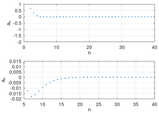
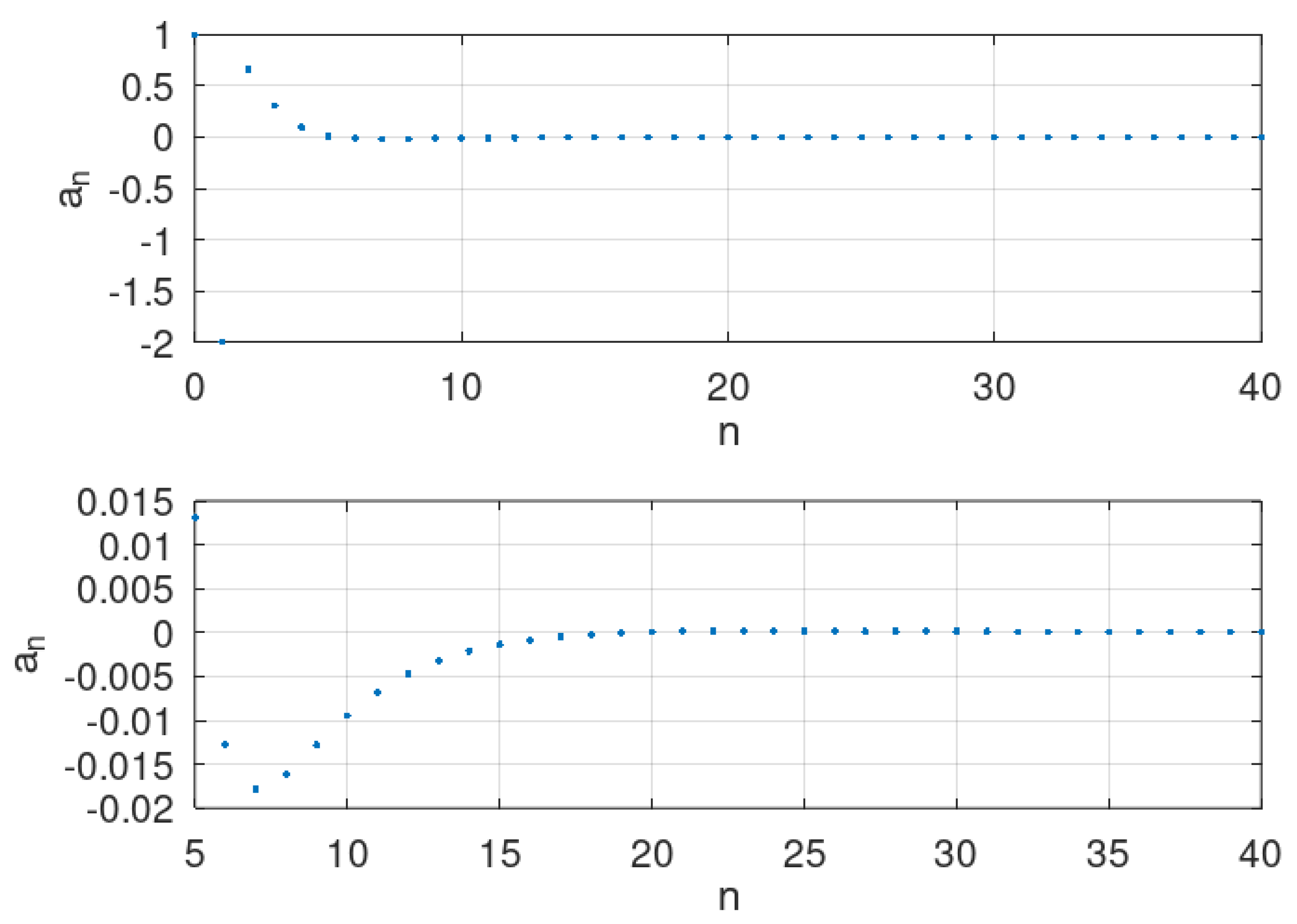
In the upper strip in the following picture (Figure 1), we depict this sequence. To see how fast it decreases, we plot the sequence for $n=5,6,7,\cdots$. The value for $n=5$ is $\approx 0.0013$ and for $n=20$ is $\approx 6\times {10}^{-5}$.

Figure 1. Numerical computation of $a_n,n=0,1,2,\cdots$ (upper strip); in the (lower strip) a zoom of the sequence, $a_n,n=5,6,7,\cdots$, is depicted.

As the sequence of coefficients decreases to zero, and $\left|z\right|<1$, the series (20) converges uniformly for every $t>0$. □

Corollary 2.

Under the conditions of the previous theorem,

$$\sum _{k=0}^{\infty }{a}_k=0.$$

(24)

This very important result is a consequence of the fact that $\underset{t\to 0}{lim}g\left(t\right)=0.$

Therefore, we can write

$$f\left(t\right)=\frac{1}{\sqrt{2\pi }\sigma t}exp\left[-\frac{{ln}^{2}t}{2{\sigma }^2}\right]=\frac{1}{\sqrt{2\pi }\sigma t}\sum _{k=0}^{\infty }{a}_k{\left[{\displaystyle \frac{t-1}{t+1}}\right]}^{2k},t\in {\mathbb{R}}^{+}.$$

(25)

3.2. The Laplace Transform of the Bilinear Function

To continue, we compute the LT of the bilinear function.

Theorem 3.

The LT of

$$h_1\left(t\right)={\left(\frac{t-1}{t+1}\right)}^{}u\left(t\right),t\in \mathbb{R},$$

(26)

where $u\left(t\right)$ is the Heaviside unit step, is given by

$$H_1\left(s\right)={\displaystyle \frac{1}{s}}-2E_1\left(s\right),Re\left(s\right)>0,$$

(27)

with

$$E_1\left(s\right)={\int }_0^{\infty }\frac{1}{t+1}{e}^{-st}\mathrm{d}t,Re\left(s\right)>0,$$

(28)

which can be easily expressed in terms of the exponential integral of order 1.

Proof. 

To obtain (27) we only have to note that

$$h_1\left(t\right)=u\left(t\right)-\frac{2}{t+1}u\left(t\right),$$

(29)

and apply the BLT. □

The function $E_1\left(s\right)$ can assume the form [16]

$$E_1\left(s\right)=e^s{\int }_1^{\infty }\frac{1}{t+1}{e}^{-st}\mathrm{d}t=-e^s\left[\gamma +lns+\sum _{n=1}^{\infty }\frac{{(-1)}^n{s}^n}{nn!}\right],Re\left(s\right)>0,$$

(30)

where $\gamma =0.5772156649$ is the Euler’s constant.

Corollary 3.

Let $N>0$ be an integer number and

$$h_N\left(t\right)={\left(\frac{t-1}{t+1}\right)}^{N}u\left(t\right).$$

(31)

Its LT is given by

$$H_N\left(s\right)={\displaystyle \frac{1}{s}}+\sum _{k=1}^N{\displaystyle \frac{{(-N)}_k}{k!}}{2}^k{E}_k\left(s\right),$$

(32)

with ${\left(a\right)}_n=a(a+1)\cdots (a+n-1),m=0,1,\cdots ,{\left(a\right)}_0=1$ being the Pochhammer symbol for the raising factorial and

$$E_k\left(s\right)={\int }_0^{\infty }\frac{1}{{(t+1)}^k}{e}^{-st}\mathrm{d}t,Re\left(s\right)>0,$$

(33)

related to the $k^{th}$ order exponential integral [16].

The proof is immediate; by using (29) and the binomial theorem, with ${(-1)}^k\left(\genfrac{}{}{0pt}{}{N}{k}\right)=\frac{{(-N)}_k}{k!},k=0,1,\cdots ,N$, we obtain

$$h_N\left(t\right)=\sum _{k=0}^N{\displaystyle \frac{{(-N)}_k}{k!}}{\displaystyle \frac{2^k}{{(t+1)}^k}},$$

(34)

to which we apply the LT. It is possible to relate $E_k\left(s\right)$ and $E_1\left(s\right)$ as we will see in the following.

Theorem 4.

Let $E_k\left(s\right)$ be as in (33). It can be expressed as

$$E_{k+1}\left(s\right)={(-1)}^k{\displaystyle \frac{s^k}{k!}}{E}_1\left(s\right)-{\displaystyle \frac{1}{k!}}\sum _{m=0}^{k-1}{(-1)}^{m}m!s^{k-1-m},Re\left(s\right)>0.$$

(35)

Proof. 

The repeated derivative computation of ${\displaystyle \frac{1}{t+1}}u\left(t\right)$ leads to

$${\displaystyle \frac{d^k}{d{t}^k}}\left[{\displaystyle \frac{1}{t+1}}u\left(t\right)\right]={(-1)}^k{\displaystyle \frac{k!}{{(t+1)}^{k+1}}}u\left(t\right)+\sum _{m=0}^{k-1}{(-1)}^m(k-1-m)!{\delta }^{\left(m\right)}\left(t\right)$$

and

$${\displaystyle \frac{1}{{(t+1)}^{k+1}}}u\left(t\right)={\displaystyle \frac{{(-1)}^k}{k!}}{\displaystyle \frac{d^k}{d{t}^k}}\left[{\displaystyle \frac{1}{t+1}}u\left(t\right)\right]-{\displaystyle \frac{1}{k!}}\sum _{m=0}^{k-1}{(-1)}^{m}m!{\delta }^{(k-1-m)}\left(t\right).$$

(36)

Applying the LT and using the derivative property [12], we obtain (35). □

With this result, we can give a new form to (32),

$$H_N\left(s\right)={\displaystyle \frac{1}{s}}+E_1\left(s\right)\sum _{k=1}^N{(-1)}^k{\displaystyle \frac{{(-N)}_k}{k!}}{2}^k{\displaystyle \frac{s^k}{k!}}-\sum _{k=1}^N{\displaystyle \frac{1}{k!}}{\displaystyle \frac{{(-N)}_k}{k!}}{2}^k\sum _{m=0}^{k-1}{(-1)}^{m}m!s^{k-1-m}.$$

(37)

This transform is not relevant to the following. Therefore, we will leave it.

It is important to remark that (34) is nothing else than a partial fraction decomposition of $h_N\left(t\right)$ that can be used to obtain the decomposition of the function

$$q_N\left(t\right)={\displaystyle \frac{1}{t}}{\left(\frac{t-1}{t+1}\right)}^{N}u\left(t\right).$$

(38)

However, we will follow a different procedure.

Theorem 5.

Let $N\in {\mathbb{Z}}_0^{+}$. Then, for $t>0$,

$$q_N\left(t\right)={\displaystyle \frac{{(-1)}^N}{t}}+\sum _{k=1}^N{\displaystyle \frac{A_k}{{(t+1)}^k}},$$

(39)

where

$$A_{N-m}=-{(-1)}^N\sum _{k=0}^m{\displaystyle \frac{{(-N)}_k}{k!}}{2}^{N-k}.$$

(40)

Proof. 

The formula (39) comes directly from the residue computation and the use of the product deriative’s Leibniz rule. In fact, from the residue theorem, we can write [17]

$$A_{N-m}={\displaystyle \frac{1}{m!}}{\displaystyle \frac{d^m}{d{t}^m}}{\left[{\displaystyle \frac{{(t-1)}^N}{t}}\right]}_{t=-1}={\displaystyle \frac{1}{m!}}{\left.\sum _{k=0}^m{\displaystyle \frac{m!}{(m-k)!k!}}{\displaystyle \frac{d^k{(t-1)}^N}{d{t}^k}}{\displaystyle \frac{d^{m-k}{t}^{-1}}{d{t}^{m-k}}}\right|}_{t=-1},$$

from where we obtain (40). □

The second term in (39) is a polynomial in ${(t+1)}^{-1}$. The coefficients of the lower order polynomials are

$$\left|\begin{array}{c}1\hfill \\ 2\hfill \\ 3\hfill \\ 4\hfill \\ 5\hfill \\ 6\hfill \end{array}\right|\left.\begin{array}{cccccc}2& & & & & \\ 0& -4& & & & \\ 2& -4& 8& & & & \\ 0& -8& 16& -16& & \\ 2& -8& 32& -48& 32& \\ 0& -12& 48& -112& 128& -64\end{array}\right|$$

Letting ${\overline{A}}_{N-m}={\sum }_{k=0}^m{\displaystyle \frac{{(-N)}_k}{k!}}{2}^{N-k},$ we obtain:

$${\overline{A}}_N=2^N,$$

$${\overline{A}}_{N-m}={\overline{A}}_{N-m+1}+{\displaystyle \frac{{(-N)}_m}{m!}}{2}^{N-m},m=1,2,\cdots$$

For $m=N-1$, we obtain

$${\overline{A}}_1=\sum _{k=0}^{N-1}{\displaystyle \frac{{(-N)}_k}{k!}}{2}^{N-k}=2^N\sum _{k=0}^N{\displaystyle \frac{{(-N)}_k}{k!}}{2}^{-k}-{\displaystyle \frac{{(-N)}_N}{N!}},$$

and

$$A_1=-{(-1)}^N\left(2^N{(1-\frac{1}{2})}^N-{\displaystyle \frac{{(-N)}_N}{N!}}\right)=-{(-1)}^N(1-{(-1)}^N)=\left(1-{(-1)}^N\right),$$

(41)

an interesting result that will be used later, because it has a deep influence on the final result.

Recursions in order can be found easily. As

$${\displaystyle \frac{1}{t(t+1)}}={\displaystyle \frac{1}{t}}-{\displaystyle \frac{1}{t+1}},$$

and

$$q_{N+1}\left(t\right)=q_N\left(t\right)\left(1-{\displaystyle \frac{2}{t+1}}\right),$$

we are led to

$${\displaystyle \frac{-{(-1)}^N}{t}}+\sum _{k=1}^{N+1}{\displaystyle \frac{A_k^{N+1}}{{(t+1)}^k}}={\displaystyle \frac{{(-1)}^N}{t}}+\sum _{k=1}^N{\displaystyle \frac{A_k^N}{{(t+1)}^k}}-{\displaystyle \frac{2}{t+1}}\left({\displaystyle \frac{{(-1)}^N}{t}}+\sum _{k=1}^N{\displaystyle \frac{A_k^N}{{(t+1)}^k}}\right),$$

where the superscript represents the order of the recursion. Then,

$$\sum _{k=1}^{N+1}{\displaystyle \frac{A_k^{N+1}}{{(t+1)}^k}}={(-1)}^N{\displaystyle \frac{2}{t+1}}+\sum _{k=1}^N{\displaystyle \frac{A_k^N}{{(t+1)}^k}}-2\sum _{k=1}^N{\displaystyle \frac{A_k^N}{{(t+1)}^{k+1}}},$$

which gives the recursive relation

$$A_k^{N+1}=A_k^N-2A_{k-1}^N,k=2,3,\cdots ,N,$$

(42)

with

$$A_{N+1}^{N+1}=-2A_{N-1}^N.$$

As a consequence,

$$A_k^{N+2}=A_k^N-4A_{k-1}^N+A_{k-2}^N,k=3,4,\cdots ,N$$

(43)

with

$$A_2^{N+2}=A_2^N-4,$$

$$A_{N+1}^{N+2}=-4A_N^N+A_{N-1}^N,$$

$$A_{N+2}^{N+2}=4A_N^N=2^{N+2}.$$

3.3. A New Series for the Lognormal Distribution

The above results show that, for an even order, $2N$, the case we are interested in, we obtain the decomposition

$$q_{2N}\left(t\right)={\displaystyle \frac{1}{t}}+\sum _{k=2}^{2N}{\displaystyle \frac{A_k^{2N}}{{(t+1)}^k}},$$

(44)

since the terms in ${\displaystyle \frac{1}{t+1}}$ disappear, because the coefficients, $A_1^N,N=0,2,4,\cdots ,$ are always null, from (41).

Theorem 6.

The lognormal distribution is represented, for $t>0$, by the series

$$f\left(t\right)=\frac{1}{\sqrt{2\pi }\sigma }\sum _{n=1}^{\infty }{a}_n{\overline{q}}_{2n}\left(t\right),$$

(45)

with the $a_n,n=1,2,\cdots$ given by (22) and

$${\overline{q}}_{2n}\left(t\right)=\sum _{k=2}^{2n}{\displaystyle \frac{A_k^{2n}}{{(t+1)}^k}}.$$

(46)

Proof. 

It is enough to attend to (24) to conclude that the partial fractions in ${\displaystyle \frac{1}{t}}$ do not appear. □

Attending to (38) and to (44), we can write

$${\overline{q}}_{2n}\left(t\right)=\sum _{k=2}^{2n}{\displaystyle \frac{A_k^{2n}}{{(t+1)}^k}}=2\sum _{k=0}^{n-1}\left(\genfrac{}{}{0pt}{}{2n}{2k+1}\right){\displaystyle \frac{t^{2k}}{{(t+1)}^{2n}}}.$$

(47)

The second expression on the right is better than the first from a numerical point of view.

Remark 2.

Given the form of the relation (45),

$$f\left(t\right)=\frac{1}{\sqrt{2\pi }\sigma }\sum _{n=1}^{\infty }{a}_n\sum _{k=2}^{2n}{\displaystyle \frac{A_k^{2n}}{{(t+1)}^k}},$$

we would be tempted to invert the order of summation, to obtain a Laurent series

$$f\left(t\right)=\frac{1}{\sqrt{2\pi }\sigma }\sum _{k=2}^{\infty }{B}_k{\displaystyle \frac{1}{{(t+1)}^k}},$$

(48)

with $B_k=\left[{\sum }_{n=k}^{\infty }{a}_n{A}_k^{2n}\right].$ The problem is in the fact that sequence $A_k^{2n},n=1,2,\cdots$ increases faster than $a_n,n=1,2,\cdots$, and the series does not converge. It is also interesting to see that, if it converged, then, it would be simple to show that the convolution of two LGN distributions is a LGN distribution. This result is a consequence of the fact that

$${\int }_0^t{\displaystyle \frac{1}{{(\tau +1)}^k}}{\displaystyle \frac{1}{{(t-\tau +1)}^n}}\mathrm{d}\tau ,k,n\ge 2,$$

is a linear combination of fractions of the type ${\displaystyle \frac{1}{{(t+1)}^k}},k\ge 2.$ This result allows us to understand why the lower summation limit in (48) is 2. If it was less than two, the convolution would not be of the same type, and the corollary would not be valid. However, this reasoning remains valid if we consider (45).

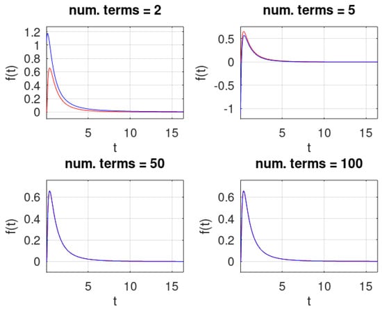
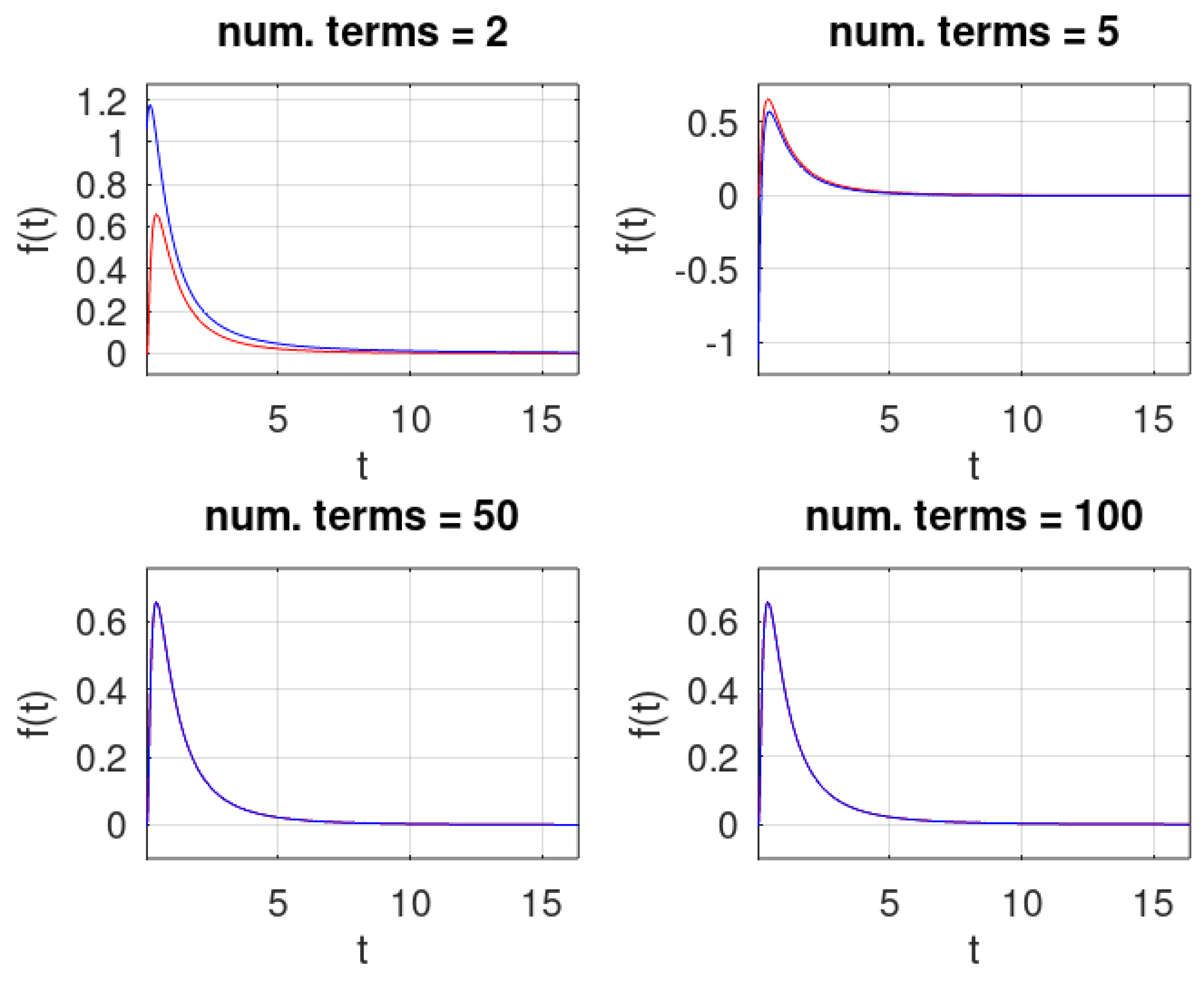
In Figure 2, we depict four approximations to the LGN function using (45). There is no visible difference between the approximations for 50 and 100 terms. This is confirmed by the square approximation errors that are around $5\times {10}^{-6}$.

Figure 2. Numerical computation of $f\left(t\right)$ (45) for $2,5,50,$ and 100 terms of the series.

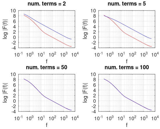
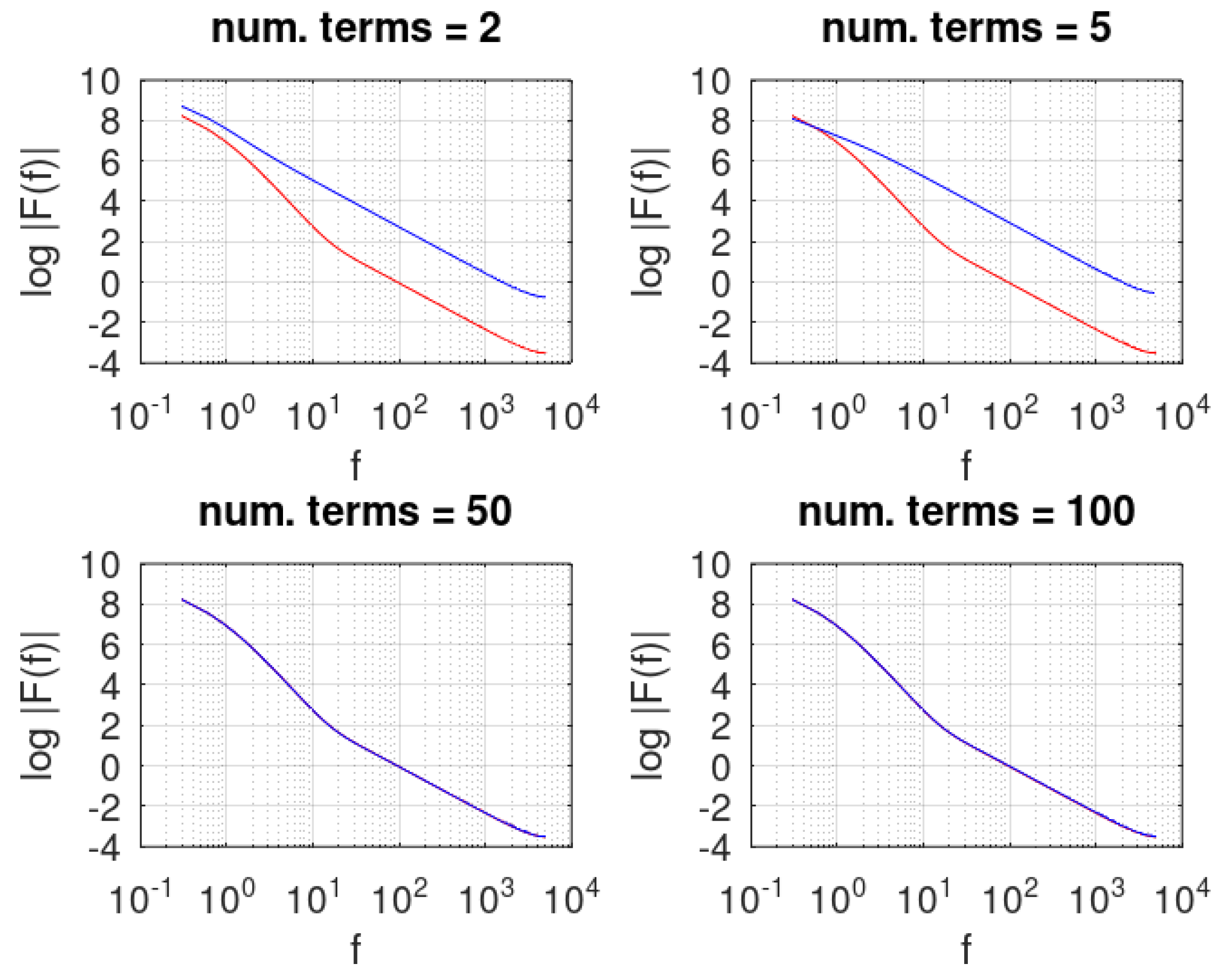
To make another fair comparison, we computed the FT of the resulting functions. In Figure 3, we present the corresponding absolute values on a logarithmic scale. A sampling interval equal to $0.0001$ was used to obtain the sampled signal that was transformed using the fast Fourier transform with length $2^{15}$. The red line represents the spectrum of the sampled signal obtained from (1).

Figure 3. Numerical computation of the FT, $F=\mathcal{F}\left[f\left(t\right)\right]$ for the approximate functions depicted in Figure 2.

3.4. The LT of the Lognormal Distribution

Let us return to (46) and use (36) to obtain

$${\overline{q}}_{2n}\left(t\right)=\sum _{k=1}^{2n-1}{A}_{k+1}^{2n}\left[{\displaystyle \frac{{(-1)}^k}{k!}}{\displaystyle \frac{d^k}{d{t}^k}}\left[{\displaystyle \frac{1}{t+1}}u\left(t\right)\right]-{\displaystyle \frac{1}{k!}}\sum _{m=0}^{k-1}{(-1)}^{m}m!{\delta }^{(k-1-m)}\left(t\right)\right],$$

whose LT is

$${\overline{Q}}_{2n}\left(s\right)=\sum _{k=1}^{2n-1}{A}_{k+1}^{2n}\left[E_1\left(s\right){\displaystyle \frac{{(-1)}^k{s}^k}{k!}}-{\displaystyle \frac{1}{k!}}\sum _{m=0}^{k-1}{(-1)}^{m}m!s^{k-1-m}\right],$$

which can be written as

$${\overline{Q}}_{2n}\left(s\right)=E_1\left(s\right)\sum _{k=1}^{2n-1}{A}_{k+1}^{2n}{\displaystyle \frac{{(-1)}^k{s}^k}{k!}}-\sum _{k=1}^{2n-1}{A}_{k+1}^{2n}\sum _{m=0}^{k-1}{(-1)}^m{\displaystyle \frac{m!}{k!}}{s}^{k-1-m}.$$

(49)

As $E_1\left(s\right)$ tends to infinity logarithmically when $s\to 0$, the other terms term tend to zero, which implies, by the final value theorem, that ${\overline{q}}_{2n}(\infty )=0.$ This is coherent with our knowledge of the function. The initial value theorem is not easy to apply.

Theorem 7.

The LT of the lognormal distribution (45) is given by

$$F\left(s\right)=\frac{1}{\sqrt{2\pi }\sigma }\left[E_1\left(s\right)\sum _{n=2}^{\infty }{a}_n{P}_1^n\left(s\right)-\sum _{n=2}^{\infty }{a}_n{P}_2^n\left(s\right)\right],$$

(50)

where $P_1^n\left(s\right)$ and $P_2^n\left(s\right)$ are polynomials given respectively by

$$P_1^n\left(s\right)=\sum _{k=1}^{2n-1}{A}_{k+1}^{2n}\left[{(-1)}^k{\displaystyle \frac{s^k}{k!}}\right],$$

and

$$P_2^n\left(s\right)=\sum _{k=1}^{2n-1}{A}_{k+1}^{2n}{\displaystyle \frac{1}{k!}}\sum _{m=0}^{k-1}{(-1)}^m(k-1-m)!s^m.$$

Proof. 

This result comes directly from (48) and (35). □

We must note that the first term on the right-hand side in (50) is the product of two functions with very different analytic behavior: the first, $E_1\left(s\right)$, has the region of convergence defined by $Re\left(s\right)>0$, while the second is holomorphic and assumes the form of a Taylor polynomial. Therefore, the main important behavior of the LGN distribution is imposed by $E_1\left(s\right)$. Since this function is not regular at the origin, the characteristic function cannot be used to define the moments of the distribution.

4. Conclusions

In this paper, we aimed to find the Laplace transform of the lognormal distribution. We proceeded in steps, starting from a first series representation in terms of the bilinear function, from where we obtained a simplified version, from where we obtained the transform. Let us balance the gains and losses by moving from representation (1) to (25):

• $f\left(x\right)$ is represented in (1) by a composition involving two transcendental functions, while in (25), it is defined through a series with only algebraic terms.
• With (25) we can approximate $f\left(x\right)$ with a finite number of terms.

Passing from (25) to (45) provided us with the following:

• The series in (45) has simpler terms that have LT. Thus, the series can be transformed term by term.
• The convolution of two LGN functions is a difficult task when using representation (1), but it is simple using (45), since the convolution of two functions of the type $\frac{1}{{(t+1)}^k}u\left(t\right),k=2,3,4,\cdots$ is a linear combination of functions of the same type.

From the final result stated in (50), we can say that

• It is very curious, since it expresses the LT of the LGN as the difference of two functions: one is analytic in the right half complex plane, while the other is holomorphic.
• The LT initial value theorem tells us that the two terms must tend mutually asymptotically on the real axis, since they have polynomial behavior and the initial value is zero.
• Although interesting from a theoretical point of view, it is not very useful for numerical implementations due to the presence of the factorial function that causes the appearance of numerical overflows.

It may be that the two terms have particular meaning relative to probability theory.

References

- Cramér, H. The Elements of Probability Theory and Some of Its Applications; John Wiley & Sons: New York, NY, USA; Chapman & Hall Ltd.: London, UK, 1955. [Google Scholar]
- Pratesi, M.; Santucci, F.; Graziosi, F.; Ruggieri, M. Outage analysis in mobile radio systems with generically correlated log-normal interferers. IEEE Trans. Commun. 2000, 48, 381–385. [Google Scholar] [CrossRef] [Scilit]
- Laourine, A.; Stephenne, A.; Affes, S. Estimating the Ergodic Capacity of Log-Normal Channels. IEEE Commun. Lett. 2007, 11, 568–570. [Google Scholar] [CrossRef] [Scilit]
- Ai, J.; Qi, X.; Yu, W.; Deng, Y.; Liu, F.; Shi, L. A New CFAR Ship Detection Algorithm Based on 2-D Joint Log-Normal Distribution in SAR Images. IEEE Geosci. Remote Sens. Lett. 2010, 7, 806–810. [Google Scholar] [CrossRef] [Scilit]
- Li, J.; Zhou, Q.; Yeh, W.W.G. A Bayesian hierarchical model for estimating the statistical parameters in a three-parameter log-normal distribution for monthly average streamflows. J. Hydrol. 2020, 591, 125265. [Google Scholar] [CrossRef] [Scilit]
- Zuo, R.; Wang, J.; Xiong, Y.; Wang, Z. The processing methods of geochemical exploration data: Past, present, and future. Appl. Geochem. 2021, 132, 105072. [Google Scholar] [CrossRef] [Scilit]
- Limpert, E.; Stahel, W.A.; Abbt, M. Log-normal Distributions across the Sciences: Keys and Clues. BioScience 2001, 51, 341–352. Available online: https://academic.oup.com/bioscience/article-pdf/51/5/341/26891292/51-5-341.pdf (accessed on 15 July 2022). [CrossRef] [Scilit]
- Leipnik, R.B. On lognormal random variables: I-the characteristic function. ANZIAM J. 1991, 32, 327–347. [Google Scholar] [CrossRef] [Scilit]
- Beaulieu, N.C. A power series expansion for the truncated lognormal characteristic function. In Proceedings of the 2010 25th Biennial Symposium on Communications, Kingston, ON, Canada, 12–14 May 2010; pp. 284–287. [Google Scholar]
- Asmussen, S.; Jensen, J.L.; Rojas-Nandayapa, L. On the Laplace Transform of the Lognormal Distribution. Methodol. Comput. Appl. Probab. 2016, 18, 441–458. [Google Scholar] [CrossRef] [Scilit]
- Miles, J. On the Laplace transform of the lognormal distribution: Analytic continuation and series approximations. J. Comput. Appl. Math. 2022, 404, 113904. [Google Scholar] [CrossRef] [Scilit]
- Ortigueira, M.D.; Machado, J.T. Revisiting the 1D and 2D Laplace transforms. Mathematics 2020, 8, 1330. [Google Scholar] [CrossRef] [Scilit]
- Deakin, M.A. The Laplace transform of exp (et). ANZIAM J. 1996, 37, 279–287. [Google Scholar] [CrossRef] [Scilit]
- Boyadzhiev, K.N. A series transformation formula and related polynomials. Int. J. Math. Math. Sci. 2005, 2005, 3849–3866. [Google Scholar] [CrossRef] [Scilit]
- Papoulis, A. The Fourier Integral and Its Applications; Polytechnic Institute of Brooklyn, McCraw-Hill Book Company Inc.: New York, NY, USA, 1962. [Google Scholar]
- Abramowitz, M.; Stegun, I.A. Handbook of Mathematical Functions with Formulas, Graphs, and Mathematical Tables; US Government Printing Office: Washington, DC, USA, 1964; Volume 55.
- Oppenheim, A.V.; Willsky, A.S.; Hamid, S. Signals and Systems, 2nd ed.; Prentice-Hall: Upper Saddle River, NJ, USA, 1997. [Google Scholar]
Publisher’s Note: MDPI stays neutral with regard to jurisdictional claims in published maps and institutional affiliations. |
© 2022 by the author. Licensee MDPI, Basel, Switzerland. This article is an open access article distributed under the terms and conditions of the Creative Commons Attribution (CC BY) license (https://creativecommons.org/licenses/by/4.0/).