


Abstract
As bandwidth-intensive applications proliferate and the usage of wireless devices surges, fifth-generation (5G) and beyond (B5G) networks are challenged to enhance coverage, reduce latency, and improve efficiency. The application of machine learning (ML) models for received signal strength (RSS) estimation is a powerful tool. This study evaluates various ML models—categorical boosting (CatBoost), extreme randomized trees (ETs), light gradient boosting machine (LGBM), and extreme gradient boosting (XGBoost)—for effective estimation of RSS. Additionally, we apply explainable artificial intelligence (XAI) methodologies, especially the Shapley additive explanation (SHAP) framework. Our investigation reveals the sophisticated mechanisms within these models, notably highlighting the exceptional accuracy of the ET model. We further introduce SHAPRP, in which SHAP attributions reduce the input space and sparse regression selects a compact subset of the ET ensemble. The results are obtained from a single-operator rural/semi-rural campaign and constitute a case study, where the trained estimator is deployment-specific and is not a pre-trained model applicable to arbitrary 5G/B5G scenarios, so what transfers is SHAPRP itself.
1. Introduction
Recent advances in telecommunications, with the implementation of 5G networks aimed at improving the performance of 4G networks, have highlighted the crucial role of radio propagation modeling in the strategic deployment and optimization of network infrastructures. Accurate and advanced models are essential to assess path loss (PL) or received signal strength (RSS) [1,2,3]. These evaluations are vital for optimizing cell coverage, strategically placing base stations, and improving network performance in different environments. They are key to creating detailed radio coverage maps and implementing advanced localization solutions [4,5,6].
Traditional RSS estimation methods mainly use ray tracing (RT) or stochastic models. RT models, which are grounded in physical principles and enhanced by empirical data, are computationally intensive and perform well in simple environments such as open terrains with clear weather [7,8]. However, in complex urban areas with many obstacles, RT requires significant additional computational resources to perform accurate modeling. Stochastic models, despite their effectiveness, often perform poorly in complex scenarios due to their limited capacity to take advantage of environmental data, resulting in reduced precision [6,9].
To address the shortcomings of traditional propagation models, AI and ML techniques are emerging as powerful alternatives. ML-based models should not be viewed as direct replacements for deterministic methods such as ray tracing (RT). RT remains valuable when accurate environmental descriptions and physically grounded propagation estimates are required. ML models are complementary data-driven estimators that can learn empirical relationships from representative measurements or simulations and provide fast inference after training. ML and deep learning (DL) are increasingly used in wireless networking due to their ability to learn complex relationships among variables that are difficult to analyze directly [10]. These techniques focus on estimating RSS and PL in wireless communications, treating them as a regression-based supervised learning problem characterized by continuous target variables and designated channel features. This use of ML and DL helps uncover data interdependencies and enhances network performance [11,12,13,14,15,16].
The main challenge with ML models is achieving a balance between complexity and accuracy, which has spurred developments in explainable artificial intelligence (XAI). XAI tailors explanations to model complexity, estimation scope, and user expertise, evaluating explanation effectiveness and addressing shortcomings to adhere to principles like equity, data privacy, and causality. XAI’s localized and holistic insights enhance model transparency and accountability, increase user trust, and allow systematic improvements [17].
A prominent contribution in the domain of ensemble learning is the adaptive deep forest shrinkage (ADeFS) [18]. This framework utilizes deep forest architectures augmented with regularization techniques such as Lasso and ElasticNet to enhance regression accuracy while simultaneously reducing model complexity. Despite its effectiveness, ADeFS is inherently designed for high-capacity ensemble systems, such as models composed of many base estimators, such as a large number of trees or multiple forest layers, which makes it less appropriate for deployment in resource-constrained environments where computational and memory limitations are critical considerations.
1.1. Motivation and Contributions
Accurate RSS estimation constitutes a critical task in the optimization and control of 5G and B5G communication infrastructures. ML is useful in wireless channel estimation when representative measurement or simulation data are available and the relationship between propagation conditions and target variables is difficult to express with a simple closed-form model. Although ensemble-based ML architectures have demonstrated commendable predictive capabilities, their inherent complexity, memory overhead, and limited interpretability hinder their suitability for deployment in edge and IoT environments, where computational and energy constraints are pronounced.
This paper proposes SHAPRP, a two-stage framework for compact and interpretable RSS estimation. In the first stage, SHAP values are used to rank the input features and select a reduced subset of stable and informative variables. In the second stage, the outputs of individual ET trees are treated as regressors and compressed using Lasso, ElasticNet, and Adaptive Lasso. The final model is therefore smaller, faster, and still interpretable through post-pruning SHAP recalculation.
Most existing RSS estimation studies focus mainly on improving accuracy. Less attention has been given to models that are accurate, interpretable, and compact at the same time. This is important for edge and embedded wireless applications, where memory, latency, and transparency are practical constraints.
The motivation for this work stems from the need for RSS estimators that are not only accurate, but also compact, interpretable, and suitable for deployment in resource-constrained wireless monitoring systems. The contribution of this paper is the design and validation of a deployment-oriented RSS estimation pipeline that uses these tools in a structured way. In the proposed SHAPRP framework, SHAP is first used as an operational feature-reduction mechanism, not only as a post hoc visualization tool. The stability of the selected feature subset is then assessed through repeated train/test splits. Subsequently, sparse regression is applied at the estimator-output level, where the predictions of individual ET trees are treated as regressors and weak or redundant trees are removed.
This integration provides a specific strategy for RSS estimation: the model starts from the most accurate but computationally expensive ET baseline, reduces the input dimensionality using stable SHAP rankings, and then compresses the ensemble through Lasso, ElasticNet, and Adaptive Lasso. The resulting model explicitly links interpretability, feature reduction, and estimator-level pruning. Therefore, the novelty is not methodological invention of SHAP or Lasso, but their task-specific integration into a compact and explainable RSS estimation workflow, together with empirical validation of the resulting accuracy–complexity tradeoff. The resulting model exhibits substantial compression, improved transparency, and minimal degradation in performance, rendering it suitable for inference in constrained communication environments. The principal contributions of this work are summarized as follows:
- A deployment-oriented two-stage RSS estimation framework, SHAPRP, is proposed. The framework combines SHAP-guided feature reduction with estimator-level sparse pruning of an ET ensemble.
- The role of SHAP is extended beyond post hoc visualization. SHAP values are used to select a compact and stable subset of input variables, and the stability of this subset is evaluated using repeated train/test splits.
- Sparse regression is applied to the outputs of individual ET trees. Lasso, ElasticNet, and Adaptive Lasso are used to identify redundant estimators and remove them from the final ensemble, thereby reducing storage and inference cost.
- A systematic accuracy–complexity analysis is provided for CatBoost, LGBM, XGBoost, ET, and the pruned SHAPRP variants. The results show that the proposed approach preserves most of the ET accuracy while substantially reducing deployment cost.
- Beyond MAE, RMSE, and MAPE, the evaluation includes model size, inference latency, throughput, SHAP-ranking stability, multicollinearity analysis, knowledge-distillation comparison, and spatial holdout testing to assess deployment robustness.
- The scope of each stage is made clear: the SHAP reduction stage is relevant to any tree ensemble that allows additive attributions, while the pruning stage depends on independently trained, exchangeable members and is thus designed specifically for randomized forests.
- The pruning stage is described in theoretical terms using convexity, uniqueness, and solver convergence, while its sparsity coefficients are chosen through cross-validation instead of being set manually.
- SHAPRP is compared with knowledge distillation, post-training quantization, and naturally compact baselines, and its differences from SHAP-based selection, ensemble pruning, and ADeFS are clearly stated.
By combining XAI and model compression in a unified architecture, SHAPRP offers a scientifically grounded and practically viable solution for high-resolution RSS estimation under real-world computational constraints.
1.2. Organization of the Paper
This paper is structured as follows. Section 2 reviews the related work. Section 3 describes the measurement campaign; Section 4 explores the ML techniques, and Section 5 details the XAI techniques and the regularization methods, along with the proposed SHAPRP framework, as well as the evaluation methodology and numerical results, including model performance metrics, spatial-holdout generalization, and compression outcomes. Finally, Section 6 summarizes the key findings, the limitations of the study, and directions for future research.
Notation and Abbreviations: In this work, scalar quantities are represented by lowercase Latin symbols, while bold uppercase and lowercase characters are used to denote matrices and vectors, respectively (e.g., for matrices and for vectors).
2. Related Work
ML techniques in wireless channel modeling offer considerable benefits by effectively learning the complex interdependencies between channel parameters and environmental factors that influence signal propagation. Unlike conventional models, ML approaches can derive these relationships from real-world data, making them highly adaptable to various wireless scenarios. They can be tailored for both general assessments and specific applications, delivering accurate predictions across different environments. One notable advantage of ML models is their computational efficiency during inference: Although the training phase is resource-intensive due to large datasets, once trained, the models can quickly generate predictions with minimal computational effort. This makes ML particularly suitable for real-time applications that require fast response times. Additionally, ML models can range from simple closed-form solutions, similar to empirical models, to more complex black-box models, such as RT models, which capture intricate input-output relationships. In wireless channel modeling, ML techniques are particularly effective in predicting key parameters like RSS, crucial for optimizing network coverage and enhancing overall communication performance [1].
In ref. [19], an innovative ML framework designed to precisely estimate key wireless propagation metrics-path loss exponent (PLE), shadowing standard deviation (), and delay spread (DS)-within industrial settings is developed. This research employs a hybrid methodology that merges RT simulations with ML techniques to delve into the complex relationships between essential wireless channel metrics and environmental factors such as signal frequency, machinery size (MS) and machine density (MD). To validate this model, a comprehensive dataset from RT simulations is generated that covers 240 distinct industrial scenarios across four frequency bands: 700 MHz, 3.5 GHz, 28 GHz, and 60 GHz. This data set supports the training and evaluation of various ML models, including multilayer perceptrons (MLPs), support vector machine (SVM), and extreme gradient boosting (XGB). The methodology begins with linear regression to establish frequency-dependent trends, followed by a detailed residual analysis using MLPs that incorporate complex spatial and structural details. The MLP model stands out as the most effective, demonstrating exceptional predictive accuracy and robust generalization capabilities. Specifically, the MLP achieves impressively low RMSE values—0.05 for PLE, 0.04 dB for , and 0.03 ns for DS—highlighting its superiority in forecasting propagation behaviors across frequencies, including intermediate values such as 40 GHz, that were not part of the training data (which included only 700 MHz, 3.5 GHz, 28 GHz, and 60 GHz). This demonstrates the model’s robust generalization capability in predicting propagation parameters beyond the originally sampled frequency set.
Although the MLP model achieves low estimation errors in that study, neural-network-based solutions generally require careful hyperparameter tuning, sufficient training data, and non-negligible training cost. This makes them attractive for high-accuracy offline modeling, but their deployment cost and interpretability must be considered when the target platform is resource constrained.
The authors in [1] propose a sophisticated ML framework to enhance the accuracy of RSS estimation within stadium environments, aiming to optimize the deployment of access points for enhanced network performance. This framework utilizes a combination of RT simulations and advanced ML techniques to analyze the complex interplay between signal strength and variables such as electrical distance, defined as the transmitter–receiver separation normalized by wavelength, and the antenna gain associated with the direct propagation path. The model is based on a robust data set generated from RT simulations that encompasses a wide variety of transmitter deployments, antenna radiation profiles, and stadium architectural designs. This data set is pivotal for training and evaluating an artificial neural network (ANN), which is specifically designed to predict quickly and accurately RSS in various stadium configurations. The input feature sampling strategy improves efficiency by selecting representative combinations of transmitter locations, receiver positions, antenna patterns, and environmental configurations, thereby reducing redundant training samples while preserving the diversity needed for generalization. The proposed ANN demonstrates a remarkable capacity for generalization, accurately predicting signal strengths for transmitter arrangements, antenna designs, and stadium layouts that were not present in the training phase. It achieves low values of root mean square error (RMSE) of 0.05 dB-an indicator of its high precision and effectiveness in facilitating strategic network planning in stadium environments by pinpointing optimal locations for access points.
Liu et al. in [14] developed an innovative ML framework to estimate RSS in 5G networks at 3.5 GHz using cost-effective geographic data. This research integrates advanced ML algorithms, MLP, random forest (RF), XGBoost, and LGBM, with meticulously selected geographic characteristics to assess how urban topography and structural variables influence RSS. Utilizing a dataset derived from extensive urban field measurements, the study demonstrates the enhanced predictive power of the MLP model, which achieves a mean absolute error (MAE) of 1.2 dB and an RMSE of 1.5 dB, effectively capturing the complex dependencies between geographic attributes and RSS. Furthermore, the performance of these ML models is compared with that of traditional empirical propagation models such as the Stanford University Interim Model (SUI) and the ECC-33 model, which show higher predictive errors. This comparison underscores the enhanced precision and operational efficiency provided by the ML approach.
In ref. [20], an ML-based framework is presented for the estimation of radio signal strength in urban environments, targeting efficient transmitter placement to optimize network coverage. Using ray-tracing simulations, a dataset of signal strengths across varied urban scenarios was generated to train and evaluate predictive models. Advanced feature engineering—particularly polynomial transformations and transmitter-to-cluster distances—significantly enhanced model performance. Generalized linear models (GLMs) achieved a 77% reduction in mean absolute error (MAE), from 11.37 dB to 2.55 dB. The K-nearest neighbor (KNN) model outperformed all others, yielding the lowest MAE of 0.65 dB with minimal computational cost. The study further demonstrates that high estimation accuracy can be maintained with reduced training data, underscoring the suitability of the models for practical applications where full datasets may be unavailable.
In ref. [21], the authors investigate the use of DL models for predicting variations in RSS in device-to-device (D2D) communication links. Their analysis is based on real-world data collected at a frequency of 5.8 GHz, encompassing various environments such as indoor and outdoor line-of-sight (LOS) and non-line-of-sight (NLOS) scenarios. Several DL techniques, including Long short-term memory (LSTM), gated recurrent units (GRUs), and convolutional neural networks (CNNs), are evaluated to assess their performance in predicting RSS. In this study, the impact of channel coherence time on estimation accuracy and identifying the optimal number of input samples for accurate forecasting is explored. The results show that GRUs and LSTMs outperform CNNs, FFNs, and linear regression models, and both GRUs and LSTMs perform similarly well by effectively capturing temporal dependencies in the data. For indoor environments, the GRU and LSTM achieved an MAE of 0.72 dB and an RMSE of 1.02 dB. In outdoor settings, they delivered an MAE of 0.65 dB and an RMSE of 0.98 dB. Furthermore, the study highlights that a 25 ms input sequence is sufficient to produce reliable predictions, even for coherence times up to 23 ms. This indicates that increasing the input length beyond the coherence time does not substantially improve estimation accuracy. That study is a temporal RSS forecasting problem, whereas the present work performs feature-based RSS estimation from contextual measurements. Therefore, the sampling resolution and forecasting horizon requirements of temporal recurrent models are not directly applicable to SHAPRP.
Recent DL-based RSS and channel-estimation studies have demonstrated strong performance, especially when large-scale temporal, image-like, or multi-modal radio data are available. However, such models often require larger training sets, careful architecture selection, higher training cost, and additional compression steps before edge deployment. Since the present dataset is tabular and relatively compact, tree-based ensembles are selected as the primary modeling family because they are strong baselines for heterogeneous tabular measurements, support efficient TreeSHAP explanations, and allow direct estimator-level pruning. Alternative compression strategies, such as knowledge distillation, are also considered experimentally in this work to provide a comparison against the proposed sparse estimator-pruning strategy.
Explainable AI and Model Lightweighting
The attribution methods used here derive from the unified additive feature-attribution framework [22], in which Shapley values are the unique solution satisfying local accuracy and consistency. TreeSHAP [23] makes these values computable exactly on tree ensembles in polynomial time and provides consistent global summaries. Accuracy on trees and the consistency of the global ranking are what make SHAP usable as a selection operator, not just as a visualization. LIME [24] is model-agnostic but sampling-dependent, so aggregated global rankings are less reproducible. DeepLIFT and Integrated Gradients require differentiable models and do not apply to axis-aligned trees, while permutation importance is unstable under the feature correlation present in this dataset. Within wireless networking, XAI has so far been used mainly diagnostically [17,25], with SHAP employed as a feature-selection front-end in other domains [26,27,28]. Its use as a component that actually determines the input space of the deployed model is the gap addressed in this work.
Compression approaches fall into four families so that knowledge distillation trains a small student on the teacher’s outputs [29], with refinements transferring intermediate structure [30,31], while Quantization reduces parameter precision [32], and pruning removes components entirely. Low-rank factorization applies to dense layers, not to trees. Their applicability to tree ensembles is uneven: the serialized payload of a forest consists of split thresholds and leaf values, which are numeric, together with feature indices, child pointers, and sample counts, which are structural and not reducible by precision. Quantization is therefore limited by the width reduction of the numeric fraction alone, at best fourfold for half precision and eightfold for eight-bit leaves. Pruning has no such upper bound, and the two mechanisms can be combined. For ensembles, Zhou et al. [33] established that a chosen subset can outperform the full ensemble, and casting the selection as penalized regression makes it convex [34,35,36].
SHAPRP differs from these approaches by combining two reductions that are usually performed separately. Attribution-based selection narrows the input space but keeps the estimator the same; ensemble pruning reduces the estimator itself but works with a fixed input space, and ADeFS [18] compresses the depth of a multi-layer cascade. In SHAPRP, the first stage sets the input space that the per-tree prediction matrix of the second stage uses, so the estimators that are kept are chosen based on the reduced representation. Since the retained members are still trees trained on the original target, attributions can be recalculated on the deployed model, as shown in Section 5. Table 1 gives a summary of this comparison.
Table 1.
Positioning of SHAPRP relative to related compression and explainable-learning approaches.
Beyond RSS estimation, recent studies in SD-WAN controller placement, time-sensitive networking, and UAV network security further demonstrate that modern communication systems increasingly require models and optimization frameworks that are accurate, efficient, and suitable for deployment-constrained environments [37,38,39,40]. Although these works address different networking tasks and are not direct RSS-estimation baselines, they motivate the broader need for lightweight, interpretable, and deployment-aware network intelligence.
3. Measurement Campaign
The ML models in this work are trained and validated using empirical data from a detailed measurement campaign, a collaborative effort between Nottinghamshire County Council and Birmingham City University in the UK to improve access to the mobile network in rural areas. The campaign used a novel approach by mounting mobile devices on municipal waste collection vehicles to collect 5G signal strength data from a primary mobile network operator, namely Everything Everywhere (EE). The measurements were recorded continuously during the normal operation of the waste collection vehicles using a custom mobile application. RSS and contextual metadata were logged while the vehicles were moving along their routes; the proposed ML model itself was trained offline after data collection. This strategy made it possible to collect data from less accessible rural regions, which would typically be overlooked by conventional measurement techniques, ensuring a wide and representative sample of areas was covered.
By continuously monitoring the 5G signal in real time, this method recorded how coverage varied as vehicles passed through different locations, terrains, and environmental factors. This method ensured the collection of high-quality data essential for the refinement of ML models. The data set consists of 216,500 measurements, with 10 input parameters and one target, namely RSS, as depicted in Figure 1. The input parameters correspond to the quantities recorded by the mobile logging application. Channel quality denotes the radio-quality indicator reported by the device/application during each measurement, while GPS accuracy denotes the estimated uncertainty of the recorded geographic position. Interference was not available as a separate measured input variable in the dataset; its impact is therefore only indirectly reflected through the measured RSS and channel-quality indicators. This is a limitation of the available field measurements.
Figure 1.
ML model structure.
The feature set is restricted and does not include explicit environmental details like building footprints, building heights, terrain profiles, or any per-link blockage indicators. Some of this information is recorded indirectly: Cell ID points to the serving site and sector, which in turn encodes the transmitter’s location, sector orientation, antenna setup, and the fixed clutter within that sector. Meanwhile, Latitude and Longitude specify where the receiver is within the sector.
The high SHAP attributions for these three variables support this interpretation, and the ablation results in Section 5 indicate that Cell ID by itself is not enough and must be used together with the coordinates. Since clutter is only captured indirectly and only for the surveyed sectors, the trained estimator is suitable for interpolation within the measured deployment, not as a broadly applicable propagation model. Section 5.12 measures the loss in accuracy when extrapolation is attempted.
The measurements allow for a geographic stratification, which forms the basis of the grouped error analysis in Section 5.12. In this analysis, samples are divided into spatially separate clusters based on their coordinates, and error is reported for each cluster. These clusters cover the full morphological range of the campaign, from the densely populated regions around Nottingham and Sheffield to the more sparsely covered rural areas near the Peak District. As a result, they provide a numerical counterpart to the urban-rural contrast shown in the residual radio map of Section 5. A line-of-sight versus non-line-of-sight (LOS/NLOS) stratification cannot be performed: the dataset lacks any link-level geometry between the handset and the serving base station, as well as any visibility indicator, so such labels would need to be artificially generated and the resulting grouped errors would reflect the labelling method rather than the actual measurements. LOS/NLOS-resolved evaluation is therefore postponed to the follow-up campaign discussed in Section 6.
The dataset corresponds to one rural/semi-rural UK deployment and one operator measurement campaign. Therefore, the results should be interpreted as a detailed case study for measurement-based RSS estimation and compression, rather than as universal validation across all possible 5G/B5G environments, frequency bands, and operators. This limitation is explicitly assessed later through a spatial holdout experiment and discussed in terms of deployment generalization. The information collected offers valuable information on how the strength of the 5G signal fluctuates across various geographic areas, influenced by changing environmental conditions and time variables, providing a deeper understanding that is crucial to fine-tuning network performance and to guide future optimization efforts.
4. Baseline ML Models for RSS Estimation
This section briefly describes the role of the ML models used in the experimental comparison. The goal is not to provide a general description of each algorithm, but to clarify why these models were selected for RSS estimation and how they support the evaluation of the proposed SHAPRP framework. The selected models represent different families of tree-based ensemble learning methods, including randomized forests and gradient-boosting approaches. Ensemble learning refers to the combination of multiple base estimators to obtain a more accurate and stable model than a single learner. Its main advantage for RSS estimation is the ability to capture nonlinear interactions among geographic, network, and radio-quality variables. Its main drawback is increased memory and inference cost when many estimators are used, which directly motivates the pruning stage of SHAPRP. These models are suitable for tabular wireless measurement data because they can capture nonlinear interactions among geographic, network, and radio-quality features with limited preprocessing.
The four models were selected because they provide complementary and widely used ensemble-learning baselines for tabular regression. CatBoost was included because it is effective for heterogeneous tabular data and categorical or identifier-like inputs, such as Cell ID and Network ID. LGBM was selected as a computationally efficient gradient-boosting method that is commonly used when fast training and inference are required. XGBoost was included as a strong regularized boosting baseline with well-established performance in nonlinear regression tasks. ET was selected as a randomized forest-type ensemble because it can provide high accuracy on nonlinear tabular data and, importantly, its individual tree outputs can be directly used in the estimator-level pruning stage of SHAPRP. Therefore, these four models cover compact boosting, regularized boosting, categorical boosting, and randomized tree-ensemble learning, allowing the proposed framework to be evaluated against both efficient and high-accuracy baselines [28].
4.1. Categorical Boosting (CatBoost)
CatBoost is included as a boosting-based baseline because it can efficiently handle heterogeneous tabular data, including categorical or identifier-like variables such as Cell ID and Network ID. Its ordered target-statistics mechanism reduces target leakage when encoding categorical variables, while its symmetric tree structure provides stable and efficient inference [41,42]. In this work, CatBoost serves as a compact boosted-tree reference for comparing RSS estimation accuracy, model size, and inference latency.
4.2. Light Gradient Boosting Machine (LGBM)
LGBM is considered because it is designed for efficient gradient boosting on large tabular datasets. Its leaf-wise tree growth strategy, gradient-based one-side sampling (GOSS), and exclusive feature bundling (EFB) reduce training and inference cost while maintaining strong regression performance [43]. In the present study, LGBM represents a low-complexity boosting baseline used to examine whether a naturally compact model can provide a competitive alternative to pruning a larger ensemble.
4.3. Extreme Gradient Boosting (XGBoost)
XGBoost is included as a regularized gradient-boosting baseline. It constructs an additive ensemble of decision trees using first- and second-order loss information and includes regularization terms to control model complexity [43]. This makes XGBoost a strong benchmark for tabular regression tasks. In this work, it is used to assess whether SHAPRP-pruned ET models can preserve the accuracy advantage of a larger ensemble while approaching the efficiency of compact boosting methods.
4.4. Extremely Randomized Trees (ETs)
ET is a randomized tree-ensemble method that introduces additional randomness in feature and split selection. This can reduce variance and improve generalization on nonlinear tabular datasets [44]. In the proposed framework, ET is used as the primary base model because it provides the lowest RSS estimation error among the evaluated baselines. However, this accuracy comes with a large memory footprint and higher inference cost. Therefore, ET provides a suitable high-accuracy starting point for SHAPRP, whose purpose is to reduce the input dimensionality and prune redundant trees while preserving estimation accuracy. ET is also the natural base learner for the pruning stage: its trees are trained separately on the original target and then combined by averaging. Removing a subset results in a smaller forest of the same type, and the function class remains the same. This does not hold for boosted ensembles, in which each tree is fitted to the residuals of its predecessors, as discussed in Section 5.6.
4.5. Hyperparameter Tuning
To ensure a fair comparison among the evaluated baseline models, CatBoost, LGBM, XGBoost, and ET were tuned before the final test-set evaluation. Hyperparameter tuning was performed using Optuna, with validation RMSE used as the optimization objective. The same training and validation procedure was used for all models, and the final selected configurations were then retrained and evaluated on the held-out test set. The tuning process focused on the parameters that most directly affect the accuracy–complexity tradeoff, including the number of estimators, tree depth, learning rate, feature subsampling, leaf-size constraints, and regularization-related parameters. The selected hypeparameters for the evaluated models are presented in Table 2.
Table 2.
Selected hyperparameters of the evaluated baseline models.
The dataset is divided into training and held-out test sets in an 80/20 ratio using a fixed random seed, which ensures that all models are trained on the same training rows and evaluated on the same test rows. Each estimator reported, whether it is a baseline, the retrained reduced-feature ET, or any pruned variant, is trained only on the training partition. The cross-validation process for selecting the sparsity coefficients is performed within that partition, and the origin of the SHAP ranking is described in Section 5.1.
5. Explainable Artificial Intelligence (XAI)
The use of ML models to estimate RSS in 5G and beyond networks offers substantial performance improvements, but these models are frequently scrutinized for their limited interpretability. This “black-box” nature can hinder trust and understanding, particularly in critical applications like network optimization, where interpretability is essential for decision-making.
To enhance interpretability, we adopt explainable artificial intelligence (XAI) methods. More specifically, we apply Shapley additive explanations (SHAP), an approach derived from cooperative game theory. SHAP derives characteristic attributions by computing the Shapley value of each variable, which reflects its average marginal contribution to the model output in all possible subsets of characteristics, providing local (instance-specific) and global (dataset-wide) interpretability [25]. SHAP was selected because the proposed baseline is a tree ensemble and TreeSHAP provides efficient and consistent additive attributions for such models [22,23]. Alternative XAI methods were considered conceptually. LIME provides local surrogate explanations but is sampling-dependent and less suitable for deriving stable global feature rankings [24]. DeepLIFT and Integrated Gradients are mainly designed for differentiable neural networks and are therefore less directly applicable to ET ensembles. SHAP is thus the most appropriate choice for this work because it supports both local explanations and global feature ranking, which is required by the feature-reduction stage of SHAPRP. The role of SHAP in this work is therefore not limited to post hoc visualization; it is used as an operational component of the compression pipeline to select the feature subset that is subsequently used for retraining and estimator-level pruning [26]. For an input x, the SHAP value of the feature j is
Here, denotes the full set of input features, while denotes any subset of features that excludes feature j. The term is the model output when only the features in are used, and is the corresponding output after adding feature j.
To derive a global interpretation of feature importance, we compute the global SHAP value for each feature by averaging its absolute contribution across all data instances [25], as follows:
Here, represents the aggregated SHAP value associated with the feature j, calculated over the entire dataset comprising m observations. The absolute value is taken before averaging so that positive and negative contributions of the same feature cannot cancel; this magnitude-based form is the quantity used to rank features, while the signed attributions are retained for the directional interpretation. These global attributions provide a quantitative measure of each feature’s overall effect on the model’s RSS estimations, which helps to clarify feature importance and guide approaches for improving and optimizing the model.
By integrating SHAP into the analysis, transparency is ensured, allowing for more informed decisions in the design and optimization of wireless networks. The ability to quantify the relative contribution of each feature enhances our understanding of the behavior of the model, which is critical to improving network performance and robustness.
5.1. Feature-Selection Protocol
The global attributions used to rank the ten input variables were calculated using a tree-ensemble explainer on the entire measurement set, prior to forming the train/test split. This means the ranking had access to the data rows that would later be included in the test partition. The estimators, however, were trained solely on the training partition, and no target values from the test partition were used in fitting any model. The selection step only considered aggregate attribution statistics.
The quantity transferred is a single discrete decision, namely which four of ten columns to retain, and it is not tuned against test performance. Table 7 bounds its consequence: over repeated resamplings the top-four subset is recovered in every repetition, with Jaccard similarity 1.000, selection frequency 100%, and mean Spearman and Kendall correlations of 0.996 and 0.985. A ranking this insensitive to which rows are used would not change under a strictly partitioned computation. Computing the attributions on the training partition alone, and selecting the retained dimensionality on a held-out validation partition, is the appropriate protocol for a deployment pipeline and is adopted in the extended study of Section 6.
5.2. Estimator-Level Sparse Regression for Ensemble Compression
To achieve efficient model compression within the SHAPRP framework, we apply a suite of sparsity-inducing regularization techniques to the outputs of individual learners in the ET ensemble. In this context, ensemble compression means reducing the number of retained base estimators while preserving estimation accuracy. A weak estimator is a tree whose output contributes little to reducing the RSS estimation error, while a redundant estimator provides information already captured by other trees. Predictive fidelity is therefore interpreted as estimation accuracy, measured using MAE, RMSE, MAPE, and the additional robustness metrics reported in the numerical evaluation. The pruning problem is formulated by treating the estimation of each tree as one regressor in a sparse linear model; regularization then assigns zero or near-zero coefficients to trees that can be removed. That a subset can match the full ensemble is established by Zhou et al. [33], who showed that selecting a subset can be strictly better than retaining all members. These strategies enable selective pruning of weak or redundant predictors, thus reducing computational complexity and storage requirements while maintaining predictive fidelity.
The sparse coefficients function more as a selection mechanism than as deployment weights. The set that is kept is with , and the predictor used at deployment is simply the uniform average over the trees in this set,
So, the fitted magnitudes serve to rank the estimators, but they are not included in the deployed model, which means the compressed model is still a standard randomized forest, just with fewer trees. Using the fitted weights as deployment coefficients is an alternative discussed in Section 6.
5.2.1. Lasso-Based Selection
Lasso regression remains a cornerstone technique in high-dimensional statistical learning due to its ability to induce sparsity in parameter estimation. By applying a -norm penalty to the model coefficients, Lasso effectively performs both regularization and automatic variable selection [34]. This capability is particularly beneficial in ensemble learning, where it facilitates the removal of weak or redundant base predictors, thus promoting model interpretability and computational efficiency [18,27,45].
In the context of ensemble compression, Lasso assigns zero weights to less influential learners, thereby pruning the ensemble without substantially compromising predictive power. The penalized least squares objective governing this process is given by
Here, T denotes the total number of ensemble members, i.e., the number of individual ET trees before pruning. where N is the total number of observations, and are the observed and predicted outputs, denotes the contribution weight of the j-th ensemble member, and is a nonnegative regularization coefficient that governs the sparsity of the solution. Despite its advantages, Lasso may struggle when correlated variables are present, often selecting only one representative among them.
5.2.2. ElasticNet-Based Ensemble Refinement
To address the limitations inherent in pure regularization, particularly its instability in the presence of highly correlated variables, the ElasticNet approach augments Lasso by incorporating an additional penalty [35]. This hybrid regularization technique not only retains the sparsity benefits of Lasso but also introduces a grouping effect, allowing correlated predictors to be selected together. This is especially advantageous for ensemble pruning when redundancy is likely among learners [18,45].
The loss function optimized under ElasticNet regularization is given by
Here, and are hyperparameters that control the influence of the and penalties, respectively. The former encourages sparsity, while the latter ensures regularization stability and reduces sensitivity to data perturbations. This balance makes ElasticNet particularly robust in ensemble reduction tasks where maintaining a subset of complementary learners is desired.
5.2.3. Adaptive Lasso for Weighted Selection
The Adaptive Lasso method enhances standard Lasso by introducing feature-specific penalty weights, thereby allowing for more nuanced regularization based on prior knowledge or initial estimates. This adaptive scheme modifies the penalty by applying a lower penalty to coefficients that are deemed more significant, improving the consistency of variable selection [36].
In the ensemble learning context, Adaptive Lasso assigns weights to each learner’s contribution, favoring those with higher predictive value as determined by a preliminary estimator. The associated loss function is defined as
In this formulation, is the preliminary estimate of the j-th ensemble member’s weight, is a tuning parameter that governs the degree of adaptivity, and denotes the adaptive penalty weight. By assigning lower penalties to learners with stronger initial contributions, Adaptive Lasso selectively retains the most informative ensemble members, while discarding less useful ones. Since becomes very large as a preliminary coefficient gets close to zero, the weights are defined as with and . This limits the penalty on coefficients that are near zero without changing their order. The preliminary estimate is calculated using ordinary least squares on the per-tree prediction matrix. Since becomes very large as a preliminary coefficient gets close to zero, the weights are defined as with and . This limits the penalty on coefficients that are near zero without changing their order. The preliminary estimate is calculated using ordinary least squares on the per-tree prediction matrix. This makes it particularly effective for sparse model construction in scenarios involving a large number of base estimators.
These regularization methods are applied after model training and serve to isolate and remove weak base learners. The result is a compact and efficient ensemble, well-suited for deployment in scenarios where computational and memory resources are constrained, such as edge devices and embedded systems.
5.3. Theoretical Properties of the Pruning Stage
Once the ensemble has been trained, the selection step becomes a finite-dimensional convex program. Let represent the per-tree predictions, where , and let denote the measured RSS vector. Each of the three penalized problems can be written as
where for Lasso, for ElasticNet, and for Adaptive Lasso.
The term g is convex and differentiable, while h is convex, proper, and lower semi-continuous. This means the objective is convex and coercive, so a global minimizer exists. Because the trees of a randomized forest are correlated by construction, may be rank-deficient and the Lasso minimizer need not be unique, whereas the ElasticNet objective is strongly convex with modulus and its minimizer is unique. This provides a theoretical reason, separate from the correlation analysis, for retaining ElasticNet. Since g is L-smooth with and h has a closed-form proximal operator, the problem can be solved by proximal gradient methods, for which FISTA [46] achieves an rate in objective value. The compression stage, then, adds a one-time training cost and nothing at inference time.
Lasso identifies the correct support only when the irrepresentable condition is satisfied, which limits the correlation between the regressors that are kept and those that are discarded. This condition is unlikely to be met in a randomized forest, so it aligns with Lasso keeping a relatively large proportion of trees.
Since both the full and pruned predictors use unweighted means over their members, the compressed model is itself a randomized forest of trees. It remains an element of the same function class, not an approximation from a different one. This property allows attributions to be recomputed exactly on the deployed model using Equation (10).
5.4. Selection of the Framework Hyperparameters
The framework reveals two main quantities, namely the sparsity coefficient and the retained-feature count k. The sparsity coefficients are not manually set. For each pruning variant, the regularization path is computed over an automatically generated coefficient grid, and the operating point is chosen by five-fold cross-validation on the training partition, selecting the value that minimizes the cross-validated squared error. For ElasticNet, the mixing parameter is chosen jointly from . Estimators with fitted magnitude below are excluded. As a result, the selection of is determined by the data itself.
The value is a constant established empirically for this dataset, rather than being the result of a rule evaluated during execution. This choice comes from the ablation results reported in Section 5, where the error decreases sharply up to and then levels off, and from the stability feature ranking, where the same four features are identified in every repetition. The pipeline, as evaluated, takes k as a fixed input. The pipeline as evaluated uses k as a fixed input. For application to other datasets, this constant can instead be replaced by a criterion that is determined at run time:
so that is the fraction of the total attainable improvement contributed by the k-th feature. The retained dimensionality is then the smallest k beyond which no further feature contributes more than a tolerance ,
The rule requires that a validation partition be held out from training, is deterministic given that partition, and provides a single interpretable quantity, , to replace k itself. When applied to the curve with , it yields , which matches the elbow used in this context. Including this criterion, so that the dimensionality can be chosen automatically for a new dataset without user involvement, is a straightforward extension noted in Section 6.
5.5. SHAPRP: A SHAP-Informed Framework for Efficient and Scalable RSS Estimation
In response to the inherent trade-off between model complexity and predictive performance in ensemble architectures, we introduce SHAPRP-a compact, interpretable, and computation-aware learning framework tailored for high-fidelity RSS estimation in wireless deployment environments. Developed independently from previous ensemble selection strategies, SHAPRP is designed with deployment constraints in mind, targeting scenarios such as real-time signal estimation in edge devices, IoT nodes, and embedded communication systems.
The methodology is structured around two interdependent optimization stages designed to promote interpretability and efficiency without sacrificing accuracy. This design differs from using SHAP merely to explain a trained black-box model. In SHAPRP, SHAP directly determines the reduced input space used for retraining, while sparse regression determines which trained ET estimators remain in the deployed model. Therefore, the interpretability and compression stages are coupled: the first stage removes weak input variables, and the second stage removes weak or redundant base estimators. This provides an RSS-specific model-simplification strategy rather than a generic post hoc explanation procedure. SHAP is used for feature reduction, and sparse regression is applied to individual estimator outputs. Thus, interpretability is directly linked to structural compression rather than being used only for post hoc explanation.
- Feature Space Reduction via SHAP Attribution: This stage employs SHapley Additive exPlanations (SHAP) to quantify the contribution of each input variable to the model output, averaged across the data distribution. The features are ranked according to their global SHAP importance scores, and only the top k scores are retained. Empirical validation suggests that suffices to preserve over 98% of the original model’s performance, enabling principled dimensionality reduction (see Section 5.4).
- Ensemble Refinement through Sparse Regression: With the dimensionality-reduced dataset, the ET model is re-trained, and prediction outputs from individual trees are extracted. These outputs are treated as regressors in a second-stage model, where sparsity-enforcing regularization techniques—including Lasso, ElasticNet, and Adaptive Lasso—are applied to identify estimators with limited predictive utility. Trees corresponding to zero-valued or near-zero coefficients are subsequently pruned.
For the pruned model, SHAP values can be recomputed because the final predictor remains an additive combination of retained tree outputs. If denotes the SHAP value of feature j for tree t, then the SHAP value of the pruned ensemble is
where is the set of retained trees, consistent with Equation (3). Thus, the final compressed model remains explainable, and SHAP attributions should be recalculated after pruning when explanations of the deployed model are required. Each tree decomposes as with base value , so the base value of the pruned ensemble is and local accuracy is preserved exactly. No additional intercept appears, because the sparse coefficients are only used for selection.
Post-pruning interpretability was verified experimentally by recomputing SHAP values for the Adaptive-Lasso-pruned model and comparing the resulting feature ranking with the pre-pruning ET ranking. The ranking remained unchanged, with Spearman and Kendall rank correlations equal to 1.0. This confirms that pruning preserves the dominant explanatory structure of the original ET model rather than relying on frozen pre-pruning explanations. The general pipeline for SHAPRP continues as follows in Algorithm 1:
- Train an initial ML ensemble model using the full set of features.
- Compute global SHAP values and rank features according to importance.
- Retain the k highest-ranked features.
- Retrain the ML model on the top-k highest-ranked features.
- Select by cross-validation over the regularization path.
- Apply regularization to per-tree outputs to identify and eliminate underperforming trees.
- Recompute SHAP attributions on the pruned model.
- Deploy the resulting compressed model.
| Algorithm 1 SHAPRP |
| Require: ; retained-feature count k; threshold |
| Ensure: compressed estimator |
| 1: Split into training and test partitions (80/20, fixed seed) |
| 2: Fit ET on the training partition with all p features |
| 3: Rank features by ; top-k |
| 4: Retrain ET on |
| 5: Assemble on the training partition |
| 6: Select by 5-fold cross-validation within the training partition |
| 7: Solve the penalized problem for |
| 8: ▹ selection only |
| 9: Recompute attributions via Equation (10) |
| 10: return |
This dual-phase procedure yields models that are markedly smaller in size and exhibit reduced inference latency, yet retain predictive performance nearly equivalent to the original full-scale ensemble. Moreover, SHAPRP demonstrates the practical synergy between XAI techniques and statistical sparsification-not only enhancing model interpretability but also serving as a foundation for scalable model design. The ensemble compression methodology introduced in this work draws theoretical motivation from the ADeFS framework [18], which underscored the efficacy of sparsity-promoting regularization techniques in reducing model complexity while preserving performance. Unlike ADeFS, which is predicated on deep ensemble architectures such as multi-layered decision forests, the SHAPRP framework adopts a more streamlined and interpretable design. It employs a principled SHAP-informed pruning strategy to selectively attenuate redundancy within ET ensembles. This design choice not only enhances computational efficiency and model compactness, but also ensures that structural reductions are grounded in feature attribution analytics, thereby retaining high fidelity in predictive outcomes. The flowchart of SHAPRP is depicted in Figure 2.
Figure 2.
SHAPRP framework flowchart.
Given its compression-aware design and interpretability-driven pipeline, SHAPRP is exceptionally well-suited for intelligent sensing, adaptive communication systems, and real-time signal analytics under constrained computational budgets.
5.6. Scope of the Framework Across Ensemble Families
The two stages have different structural requirements, so their applicability should be considered separately. The SHAP reduction stage only requires that the model allows for consistent additive attributions, something TreeSHAP provides for CatBoost, LGBM, XGBoost, and also ET. This stage does not depend on how the ensemble is composed; it takes a ranking and produces a reduced set of columns, and any learner can be retrained on this set. The reduced input space is actually a feature of the estimation problem itself, not of the learner, because the dominant variables discussed in Section 5 include the serving-cell identity and the receiver position.
The pruning stage applies only to randomized ensembles, and this restriction is due to structural reasons, not empirical ones. Sparse selection over per-tree outputs assumes that the ensemble’s prediction is formed by summing terms that are each individually meaningful and can be swapped without affecting the overall structure, so that removing some and then renormalizing still gives a valid predictor for the same target.
In a randomized forest, each is fitted independently to the original target r, so each term provides its own estimate of r and the condition is satisfied exactly: any subset average remains an estimate of r, and the pruned model is simply a smaller forest of the same type. In gradient boosting, the terms are not interchangeable, since is fitted to the pseudo-residual and thus estimates a value defined by the previous trees, not the target itself. If an early tree is removed, the residual sequence used to train all subsequent trees is disrupted, so the remaining trees no longer estimate what they were originally fitted to and the ensemble is no longer an additive decomposition of r. Adjusting weights for the remaining trees can compensate for some of the bias introduced, but it cannot repair the disrupted sequence, so the accuracy declines much more rapidly with pruning than in a randomized ensemble. This outcome results from the way boosting is constructed and does not depend on the specific implementation, as it applies to XGBoost, LGBM, and CatBoost alike. The boosted baselines also do not encounter the problem that this stage is designed to solve, as they use 31.73 MB and 84.69 MB, in contrast to 1523.67 MB for ET. SHAPRP is therefore presented as a framework whose interpretability stage is suitable for tree ensembles in general, while its compression stage is aimed at large randomized ensembles. Section 6 discusses in detail how boosted ensembles are affected by the removal of estimators.
5.7. Evaluation Metrics
The estimation accuracy is evaluated using MAE, MSE, RMSE, and MAPE. MAE measures the average absolute error, RMSE penalizes larger deviations more strongly, and MAPE expresses the error relative to the measured RSS magnitude. They are defined as [47]:
and
where is the number of test samples, is the measured RSS, and is the estimated RSS. Since RSS is measured in dBm, which is a logarithmic value referenced to an arbitrary point, MAPE serves as a relative measure on that scale instead of representing a proportional error on a ratio scale. This means that a fixed dB deviation results in a different percentage depending on the absolute value. It is included for consistency with earlier RSS research, though MAE and RMSE, both in dB, provide the main interpretation. Additional deployment-oriented metrics, including model size, per-sample latency, throughput, and spatial holdout accuracy, are also reported.
5.8. Measurement Conditions for Timing and Model Size
Two distinct estimators are reported here, with the full baseline ET trained using all ten features and shown in Table 3, Table 4 and Table 5. The reduced ET, which serves as the pre-pruning reference in the pruning comparison of Section 5, is retrained on the four features selected by SHAP; each of its trees evaluates a decision path in four dimensions rather than ten, making it faster. The difference between 2.35 s and 0.50 s therefore compares two separate models and reflects the intended effect of the first stage, rather than two measurements of the same model.
Table 3.
Estimation error metrics of ML models (ten input features).
Table 4.
Inference time and model size of ML models (ten input features).
Table 5.
Accuracy–complexity comparison of baseline models (ten input features).
Model size refers to the disk space occupied by each estimator after being serialized. The sizes for all models reported in this paper are determined using this same procedure.
5.9. Numerical Results
Table 3 presents a comparative analysis of estimation error metrics for the models evaluated. To complement these results, Table 4 summarizes the computational requirements of each model, specifically the inference time and the size of the model, which are key considerations for deployment in constrained environments.
Table 3 and Table 4 reveal a clear tradeoff between estimation accuracy and computational complexity. ET provides the best RSS estimation accuracy, with the lowest MAE, RMSE, and MAPE values among the evaluated models. However, this accuracy is obtained at the cost of the highest inference time and the largest model size. In contrast, LGBM, XGBoost, and CatBoost are substantially lighter and faster, but they exhibit higher estimation errors. Therefore, the most compact baseline is not necessarily the most accurate one. This motivates the design of SHAPRP: rather than selecting a naturally compact but less accurate model, the framework starts from the most accurate ET baseline and then applies SHAP-guided feature reduction and regularization-based estimator pruning to reduce its computational burden while preserving most of its estimation accuracy.
Figure 3 shows the estimated versus real measurement values, while Figure 4a corresponds to the MAE distribution and Figure 4b to the MAPE distribution.
Figure 3.
Estimated versus real measurement values. Each dot corresponds to one test sample, and the dotted line is the identity line, along which estimated and measured values coincide.
Figure 4.
Error distributions for the ET model. Subfigure (a) reports the MAE distribution, while subfigure (b) reports the MAPE distribution.
Figure 5 presents the effect of training set size on estimation performance across all evaluated models. As the number of training samples increases, the estimation errors generally decrease, confirming that additional training data improve model generalization. However, the MAE and RMSE curves gradually flatten after a sufficiently large training subset is used, indicating diminishing accuracy gains. This suggests that beyond this region, further data collection provides limited improvement relative to the additional measurement effort.
Figure 5.
Effect of training set size on RSS estimation performance: (a) MAE in dB, (b) RMSE in dB, (c) MAPE in percent. The horizontal axis reports the number of training samples.
Furthermore, an accuracy–complexity Pareto comparison was conducted across ET, LGBM, XGBoost, and CatBoost and presented in Table 5. ET achieves the lowest error among all evaluated baselines but also the largest model size, whereas LGBM and XGBoost are substantially smaller at the cost of higher MAE. Therefore, ET is selected because it provides the highest accuracy ceiling. The objective of SHAPRP is precisely to compress this accurate but memory-intensive ensemble into a more deployment-friendly estimator. The baseline results reveal a clear accuracy–complexity tradeoff. So in this study, instead of starting from the most compact model, SHAPRP starts from the most accurate model and compresses it while preserving most of its accuracy.
The ET model exhibits better estimation accuracy than the alternative models, as evidenced by its lower MAE of dB, RMSE of dB, and MAPE of %. In comparison, LGBM and XGBoost models also demonstrate high efficacy, recording MAPE values of % and % respectively, suggesting their potential utility as alternative methodologies for RSS estimation. In contrast, the CatBoost model, while still effective, exhibits a slightly higher MAPE of %.
Figure 3 presents a scatter plot evaluating the performance of the ET model against empirical observations, with predicted results denoted by blue markers. The empirical observations represent the real RSS measurement values, while the predicted outputs correspond to the ET model’s estimations. The close clustering of points around the identity line underscores the model’s high estimation accuracy and minimal systemic deviation. The limited spread from the ideal reference, corroborated by the reduced MAPE in RSS estimation, confirms the ET model’s robustness and precision. This visualization provides compelling quantitative evidence of the ET model’s ability to accurately approximate real-world RSS behavior under varying conditions.
To further evaluate the ET model’s performance distributionally, Figure 4 illustrates the error histograms for MAE and MAPE. Both distributions exhibit a sharp concentration of values near zero, confirming the strong predictive consistency of the model and the low average deviation. The tight spread of MAPE values further indicates minimal proportional error, which is critical in real-world RSS estimation, where relative deviation may impact decision making. These error profiles reinforce the effectiveness of the ET model for high-fidelity signal prediction.
Figure 5 presents the relationship between training set size and predictive performance across all evaluated models. The observed trends substantiate each model’s ability to generalize and demonstrate that expanding the quantity of training data consistently enhances estimation accuracy. This analysis highlights the robustness of ensemble methods in delivering precise RSS estimations across various metrics, as detailed in Table 3.
The proposed ML model has the potential to create Radio maps (RMs). These maps help to visualize the spatial distributions of the RSS, thus converting theoretical data into practical insights for the evaluation of accuracy [48]. These maps classify areas according to the intensity of the signal, emphasizing RSS variations between urban and rural settings due to differences in infrastructure [49]. In addition, RMs identify coverage discrepancies, helping in the targeted enhancement of infrastructure to improve network efficiency. By correlating atypical signal patterns with environmental factors, RMs also refine the precision of predictive models and confirm data reliability [50,51].
Incorporating RMs into the analysis not only verifies ML model accuracy but also expands the actionable insights, improving the understanding of their real-world relevance. This approach highlights the importance of combining advanced visual analytics with traditional data analysis to enhance theoretical and practical knowledge, supporting smarter decision-making in telecom network planning and optimization. Furthermore, RMs play a strategic role beyond mere model validation by helping to visualize emerging demand hotspots due to urban growth and demographic changes, helping to design proactive networks and strategic planning [49,51].
The ML model does not use a RM as an input during training. Instead, the model estimates RSS values from the available measurement features, such as geographic coordinates, Cell ID, Network ID, and channel-quality indicators. The RM is then constructed after inference by spatially visualizing the measured RSS, the estimated RSS, or the residual error between them. In this work, the residual RM is used as a diagnostic and validation tool: it shows where the model overestimates or underestimates RSS across the Nottinghamshire area. Therefore, the ML model produces point-wise RSS estimates, while the RM provides a spatial interpretation of these estimates and their errors.
The residual RM shown in Figure 6 provides a detailed visualization of the variance between the predicted and actual RSS values. It employs color coding—red for positive residuals (stronger-than-expected signal strength) and blue for negative residuals (weaker-than-expected signal strength)—to highlight these differences. The map is a qualitative diagnostic where its numerical counterpart is the per-cluster error analysis of Section 5.12. This color-coding brings out several important points:
Figure 6.
Residual RSS Radio Map of Nottinghamshire area, UK. Red markers indicate positive residuals, where the measured RSS exceeds the estimated value, and blue markers indicate negative residuals.
- Urban areas with positive residuals: Clusters of positive residuals (red) in cities such as Nottingham and Sheffield indicate areas where the actual signal strength exceeds predicted levels. This overperformance might come from a dense infrastructure, beneficial signal propagation conditions, or unaccounted for variables in the model.
- Negative residual zones, especially in rural locations such as the Peak District National Park, reveal areas where the signal strength is lower than expected. These discrepancies reflect the challenges of providing consistent coverage in regions with a sparse infrastructure or natural obstacles that hinder signal propagation.
- Isolated blue and red points in unexpected areas can indicate specific issues or advantages, such as unique environmental conditions, temporary interruptions in the network, or inaccuracies in the data or model calibration.
- This residual analysis enables network operators to identify zones where the predictive model needs improvement or where infrastructure upgrades are required. These insights are crucial to address performance gaps and optimize network reliability.
The SHAP methodology improves our understanding of the predictive mechanisms within the optimal ET model. To avoid redundant visualizations, only the SHAP beeswarm plot is retained. Unlike a SHAP bar plot, which reports only mean absolute feature importance, the beeswarm plot simultaneously shows the relative importance, direction, and dispersion of each feature’s contribution to the RSS estimate. Figure 7 presents the SHAP beeswarm plot, which summarizes both global feature importance and the distribution of feature effects across individual RSS estimates. Additionally, as depicted in Table 6 the feature ablation study can retain only the most influential predictors from the SHAP analysis.
Figure 7.
SHAP beeswarm plot.
Table 6.
Performance change relative to the full 10-feature baseline.
- Cell ID denotes the identifier of the serving cellular site/sector associated with each RSS measurement. It implicitly captures deployment-specific information that is not otherwise fully represented in the input feature set, such as the serving base-station location, sector orientation, antenna configuration, transmit power, frequency configuration, and local propagation environment. RSS is strongly determined by the serving cell and its surrounding radio environment. A change in Cell ID usually corresponds to a change in the dominant transmitter and coverage region, which can lead to a substantial change in RSS values.
- Latitude and Longitude also emerge as significant contributors, emphasizing the importance of geographic factors in the model. These features influence predictions by accounting for spatial variations, which are crucial for location-based optimization in network deployments.
- Moderate influences are observed for features like Network ID and Channel Quality, which reflect the structural and operational characteristics of the network. These features are essential for capturing the dynamics of network performance and signal integrity.
- Lesser impacts from features such as GPS update time, Channel Bands, and Network Update Time suggest their secondary role in the predictive framework. However, their contributions are vital for a nuanced understanding of network behavior under various conditions.
The analysis of Latitude and Longitude underlines their critical role as geographic factors, emphasizing the need for location-specific optimization strategies. The combination of structural features like Network ID with geographic elements showcases the model’s complexity and its ability to handle intricate interactions that influence predictions.
The SHAP visualizations provide a comprehensive analysis of the elements influencing RSS estimations. The substantial effects of Cell ID, Latitude, and Longitude underscore crucial areas for network optimization to enhance the accuracy of RSS estimations in urban settings.
To evaluate the sensitivity of the SHAP-based feature selection stage, the SHAP ranking was recomputed over repeated train/test splits. The top-four subset remained unchanged in all repetitions, yielding a top-four Jaccard similarity of 1.000. The mean Spearman and Kendall rank correlations relative to the reference ranking were 0.996 and 0.985, respectively, as depicted in Table 7. These results indicate that the selected SHAP feature subset is stable under moderate data perturbations.
Table 7.
Stability of SHAP feature ranking over repeated train/test splits.
A multicollinearity analysis was also performed using pairwise Pearson correlations and variance inflation factors (VIFs). The strongest pairwise correlation was observed between GPS update time and Latitude (), while high VIF values were observed for GPS update time, Latitude, and Network Update Time. This indicates partial redundancy among some contextual variables. However, the repeated-split SHAP stability analysis showed that the top-four feature subset remained unchanged in all repetitions. Moreover, ElasticNet is included in the pruning stage because its mixed - penalty is more stable than pure Lasso when correlated predictors are present, which the strong-convexity argument of Section 5.3 also supports. The strongest observed correlation is between GPS update time and Latitude, indicating partial redundancy among contextual variables, as depicted in Figure 8. Therefore, the proposed framework does not rely solely on Lasso under multicollinearity, but evaluates Lasso, ElasticNet, and Adaptive Lasso as alternative sparsification mechanisms.
Figure 8.
Pearson correlation matrix of the input features.
To rigorously assess the computational efficiency and predictive resilience of the proposed SHAPRP framework, we conduct a two-stage experimental analysis, emphasizing its effectiveness in high-dimensional reduction and ensemble compression. This evaluation is specifically designed to validate the model’s suitability for real-time, resource-constrained deployment scenarios, such as wireless edge computing and embedded IoT systems.
The first phase focuses on feature dimensionality reduction guided by SHAP-based interpretability. As presented in Table 6, a systematic feature ablation study was performed by progressively reducing the input space to retain only the most influential predictors, as ranked by global SHAP values. The results indicate that the model sustains a high level of accuracy even when restricted to a drastically reduced feature subset. In particular, when limited to the top four features (), ET exhibits only marginal increases in MAE (1.15%) and RMSE (2.75%) compared to the full ten-feature configuration. The value was selected using an accuracy–dimensionality saturation analysis rather than assumed a priori. ET was retrained using the top k SHAP-ranked features for , and the experiment was repeated over multiple train/test splits. The largest improvement occurs when increasing from to . Beyond , the improvement becomes marginal, as presented in Table 8. As depicted in Figure 9, MAE decreases sharply up to and then saturates, supporting the selection of the top-four feature subset. Thus, is selected as the elbow point of the accuracy–dimensionality curve.
Table 8.
Effect of the number of SHAP-ranked features on ET performance.
Figure 9.
MAE: Effect of the number of retained SHAP-ranked features on RSS estimation accuracy.
Table 6 shows how much predictive information is retained when the input space is reduced according to the SHAP ranking. The results indicate that RSS estimation cannot be explained by a single feature alone. When only the top one, two, or three features are used, the error remains substantially higher than the full-feature baseline, showing that accurate RSS estimation requires both network-specific and spatial information. Although Cell ID is highly informative because it implicitly represents the serving cell and its local coverage characteristics, it must be combined with geographic features such as Latitude and Longitude to capture spatial propagation variability.
The sharp improvement from to indicates that the fourth SHAP-ranked feature provides complementary information that is not already captured by the first three features. In contrast, increasing the feature set from four to ten produces only a marginal improvement. This suggests that the remaining variables are either weakly informative, partially redundant, or already indirectly represented by the dominant cell- and location-related features. Therefore, the top-four feature subset provides an effective accuracy–complexity compromise, retaining nearly the same estimation accuracy as the full ten-feature configuration while reducing the input dimensionality.
These outcomes validate SHAP as an effective mechanism for dimensionality-aware optimization, allowing ET to operate on a compact feature set without compromising representational fidelity. This contributes to a significant reduction in computational complexity and inference latency, essential for on-device learning tasks.
The second evaluation phase addresses ensemble-level redundancy through the application of sparse regression techniques to prune underperforming estimators. Table 9 summarizes the comparative performance of Lasso, ElasticNet, and Adaptive Lasso when applied to per-tree predictions from the retrained ExtraTrees (ET) model. The reported inference times correspond to median batch inference over the test set and are also expressed as per-sample latency. The Adaptive-Lasso-pruned model achieves the lowest latency, with 0.0023 ms per sample and a throughput of approximately samples/s. SHAPRP is intended for radio-map generation, coverage monitoring, and edge-assisted network analytics, where repeated inference over large measurement grids or drive-test traces is required. These timing values are suitable for near-real-time monitoring and radio-map update tasks. Among these methods, Adaptive Lasso achieves the most aggressive compression and delivers the fastest inference time at 0.06 s. While this comes at the cost of a moderate drop in predictive accuracy (MAE = 0.95, RMSE = 2.01), the trade-off may be acceptable for latency-sensitive applications where compactness and speed are prioritized over marginal improvements in accuracy. Lasso and ElasticNet also provide substantial compression, reducing storage requirements to approximately 221–228 MB, while maintaining accuracy close to the full ET ensemble (MAE ≈ 0.90–0.91, RMSE ≈ 1.93–1.94). These results demonstrate the effectiveness of sparse linear models in achieving efficient ensemble pruning with minimal degradation in predictive performance.
Table 9.
Comparison of model metrics via pruning (four SHAP-selected features).
5.10. Knowledge Distillation Baseline
The teacher is the ET ensemble described in Table 2, trained using the four features selected by SHAP so that both the teacher and SHAPRP variants have the same input space. The student is a state architecture, layer widths or depth limit, activation, parameter count; it was designed so that its 0.175 MB size is smaller than even the most compact SHAPRP variant. Since RSS estimation is a regression task, there is no softmax and thus no temperature parameter as in classification, so none is reported here. The signal transferred is the teacher’s continuous output, and the tunable parameter is the loss weighting
where and are the teacher and student predictors, and . Training used optimizer, learning rate and schedule, batch size, epochs, early stopping, initialization, standardization, restarts, with chosen. Teacher outputs were calculated in advance on the training partition, and the test partition was reserved for the final scores.
Knowledge distillation was also evaluated as an alternative compression strategy. A compact student model was trained using the full ET ensemble as the teacher. The distilled student achieved a very small model size of 0.175 MB, but its MAE increased to 2.3400 dB and its RMSE to 4.1395 dB. In contrast, Adaptive-Lasso SHAPRP achieved MAE = 0.8653 dB and RMSE = 1.9440 dB. This indicates that estimator-level pruning preserves the behavior of the original ET ensemble more effectively than the compact distilled student for the considered RSS estimation task.
A comparison between the knowledge-distillation baselines is presented in Table 10.
Table 10.
Comparison with compact knowledge-distillation baselines.
Richer distillation schemes were evaluated for their potential use. Attention transfer [52] aligns the attention maps of intermediate convolutional layers and assumes differentiable activations with a spatial topology. Relational distillation [31] can be applied in theory, as it transfers the pairwise structure of the teacher’s output space and only needs the ability to query that space, and a similar approach for tree ensembles is found in the sample similarity that comes from leaf membership. The main limitation is the capacity of the student, and a more detailed transfer signal would likely provide an additional, second-order improvement.
5.11. Comparison with Lightweight and Quantized Baselines
The tuned LGBM and XGBoost models of Table 5 serve as naturally compact channel-prediction references, representing the alternative of choosing a small model at the outset: they occupy 31.73 MB and 84.69 MB against 1523.67 MB for ET but raise MAE from 0.87 dB to 1.190 dB and 1.296 dB. Post-training quantization is assessed analytically rather than implemented, for a reason specific to the model family. In a fitted tree ensemble, the split thresholds and leaf values are numeric and their precision can be reduced, but the feature indices, child pointers, and sample counts are structural and cannot be compressed in the same way. Thus, the achievable reduction ratio is limited by how much the numeric part can be compressed-at most, a fourfold reduction for half precision and up to eightfold for eight-bit leaves. This upper limit comes from the way the model is represented, not from any particular implementation, and it explains why reducing precision alone cannot achieve the same reductions as removing estimators. The two mechanisms are orthogonal and composable, and a joint formulation is identified in Section 6. Taken together, quantization does not affect accuracy but is limited in how much it can reduce size, distillation gives the smallest model but with the greatest accuracy loss, a naturally compact model sacrifices accuracy directly, and SHAPRP keeps most of the ET accuracy while cutting the footprint significantly, and it is the only one among the four whose deployed model remains re-explainable.
5.12. Spatial Holdout: Geographic Generalization
To assess whether the model generalizes to regions it has not seen geographically, the measurements were divided into geographic clusters using k-means on the latitude–longitude coordinates, and each cluster was left out of training in turn. Unlike random splitting, this approach ensures that no test location has a spatial neighbor in the training set, so it evaluates extrapolation instead of interpolation. Since the clusters cover the morphological range of the campaign, Table 11 also gives the per-region error breakdown, which the residual map in Figure 6 only shows in a qualitative way.
Table 11.
Spatial holdout results using geographically separated clusters.
The spatial holdout errors are much higher than those seen with random splitting, with MAE ranging from 7.69 dB to 10.51 dB and negative in every fold. The trained estimator, as a result, can interpolate within the surveyed deployment area but fails to extrapolate to regions it has not seen. This outcome is anticipated by the SHAP analysis: Cell ID is the most important feature and it carries deployment-specific information, so in a held-out cluster, it takes on values not present in the training data, while the coordinates also fall outside the training support. Any model that depends on identifier-like features will act in this way. Three consequences arise from this. First, the trained model is a deployment-specific artefact and not a general RSS predictor. Second, SHAPRP is a procedure, and it is this procedure that can be transferred, since both of its stages can be repeated on representative data from a different operator, band, or morphology. Third, deploying in a new region needs geographically varied training data or a parameterization that does not use identifiers, where Cell ID is replaced by transferable quantities like transmitter–receiver distance and relative bearing. These errors are those of the uncompressed ET baseline, so the limitation comes from the data and the way features are parameterized, not from the compression stage.
Collectively, these experimental findings affirm SHAPRP as a highly efficient, interpretable, and scalable learning framework. Its combination of SHAP-guided feature selection and regularization-driven ensemble pruning enables a principled reduction in model size and latency, all while preserving predictive reliability within the surveyed region. These properties make SHAPRP an ideal candidate for real-time RSS estimation in constrained environments, including wireless communication systems, edge computing platforms, and intelligent IoT infrastructures.
Figure 10 should be interpreted in direct comparison with Figure 3, which shows the estimated-versus-measured RSS relationship for the original ET model. The Lasso-pruned model preserves the same overall alignment around the identity line, indicating that the pruning process does not substantially alter the main RSS mapping learned by the full ET ensemble. However, the dispersion around the diagonal is slightly larger than in Figure 3, which is consistent with the moderate increase in MAE and RMSE reported in Table 9. Therefore, Figure 10 is not intended to repeat Figure 3, but to show that the compressed model maintains the dominant predictive behavior of the original ET model while using fewer effective estimators.
Figure 10.
Predicted versus measured RSS for the Lasso-pruned ET model. This figure should be compared with Figure 3 for the original ET model.
Similarly, Figure 11 showcases that most estimation errors remain concentrated near zero, confirming that the Lasso-pruned model retains the low-error behavior of the full ensemble. The distributions of the pruned model are slightly wider, reflecting the expected loss in accuracy after removing weak or redundant estimators. This comparison demonstrates the main tradeoff introduced by SHAPRP: a small degradation in error distribution is accepted in exchange for a substantial reduction in model size and inference cost.
Figure 11.
Error distributions for the Lasso-pruned ET model. This figure should be compared with Figure 4 for the original ET model.
Figure 12 compares the prediction-error metrics of the original ET model and the pruned variants obtained using Lasso, ElasticNet, and Adaptive Lasso. In this figure, the term “score” denotes the numerical value of the corresponding evaluation metric: MAE and RMSE are expressed in dB, while MAPE is expressed in percent. Thus, a lower score indicates better estimation accuracy for all three metrics. The figure shows that pruning introduces only a small increase in error compared with the original ET model, while Table 9 shows that a substantial reduction in model size and inference time accompanies this small accuracy loss. Therefore, Figure 12 should be interpreted as an accuracy-preservation comparison among the original and compressed models, rather than as a generic model score.
Figure 12.
Comparative evaluation of the original ET model and pruned variants.
Figure 13 reports the deployment complexity of the original ET model and the pruned variants using two directly measured quantities: inference time and model storage size. In this work, complexity is not defined as a hidden single score; rather, it is represented as the pair , where is the wall-clock inference time required to process the test set under the same experimental conditions, and is the serialized model size in MB. These two quantities were selected because they directly determine whether the model can be deployed in memory- and latency-constrained edge devices. The vertical axis is plotted on a logarithmic scale because the uncompressed ET model and the pruned models differ by orders of magnitude in storage size and latency.
Figure 13.
Deployment–complexity comparison of the original ET model and pruned variants. Complexity is represented by two measured quantities: inference time and serialized model size. The logarithmic scale is used because the values differ by orders of magnitude.
The percentage reduction for each complexity component is computed relative to the initial ET model as
Therefore, Figure 13 should be interpreted as a deployment-cost comparison rather than an accuracy metric. The Adaptive-Lasso variant provides the largest reduction in both storage and inference time, while Lasso and ElasticNet provide a less aggressive but still substantial reduction. When considered together with Figure 12, the complexity analysis shows the central tradeoff of SHAPRP: a small increase in estimation error is exchanged for a large decrease in deployment cost.
5.13. Deployment Considerations
Accordingly, the trained model should not be interpreted as a universal pre-trained RSS predictor for all 5G/B5G deployments. Rather, SHAPRP should be interpreted as a general compression and interpretability framework that can be retrained for other operators, environments, frequency bands, or radio technologies when representative labeled data are available. Broader validation across urban, suburban, indoor, mmWave, sub-6 GHz, multi-operator, and multi-band datasets remains an important direction for future work.
Three separate obstacles affect operator transferability. Feature-space misalignment occurs because Cell ID and Network ID are operator-specific identifiers without shared meaning, so a model that uses them cannot be transferred. Deployment-geometry shift happens when site density, sectorization, tilt, and transmit power vary between operators, even within the same area, altering the conditional distribution of RSS for a given position. Band and technology shift actually changes the underlying propagation physics. Of these, only the third is discussed in the literature, typically through frequency-scaling arguments. The first two require either retraining or explicit adaptation. In practice, for the same operator and region, periodic recalibration using a sliding window is sufficient. For different regions within the same operator, the ET stage must be retrained and the pipeline reapplied, with the main cost coming from the measurement campaign; for different operators, using a parameterization that does not rely on identifiers is essential.
Although this work focuses on RSS estimation, SHAPRP is not restricted to RSS. The same two-stage strategy can be applied to other supervised regression targets, such as SINR, throughput, latency, or QoS indicators, provided that representative labeled data and relevant contextual features are available. In such cases, SHAP would identify the dominant input variables for the target metric, while sparse estimator-level pruning would reduce the complexity of the selected ensemble model. Task-specific retraining and validation would nevertheless be required. The same principle may also be extended beyond radio-signal estimation to broader network-optimization tasks. For example, in SD-WAN controller-placement problems, SHAP-like feature attribution could help identify the most influential network-design variables while compact models support fast decision making [37]. In time-sensitive networking, lightweight interpretable models could support scheduling or routing decisions where latency and reliability constraints are critical [38,39]. Similarly, in UAV network security, explainable and compressed learning models may be useful for intrusion detection on resource-constrained aerial platforms [40]. These examples are not claimed as direct validation of SHAPRP, but they illustrate possible directions where the proposed interpretability-compression strategy could be adapted after task-specific retraining and evaluation.
In dynamic radio environments, SHAPRP can be used in an offline-training/online-inference mode, where the compressed model performs fast inference at the edge and is periodically updated as new measurements become available. Near-real-time adaptation could be implemented by periodically recomputing SHAP rankings and sparse pruning coefficients over a sliding measurement window.
From a network-integration perspective, SHAPRP can be deployed as a lightweight analytics module. In an O-RAN architecture, the compressed estimator could operate inside a near-real-time RAN Intelligent Controller xApp for radio-map updates, coverage-quality monitoring, or measurement-based optimization. In SDN/NFV systems, SHAPRP can be containerized as a virtualized analytics function that provides RSS estimates and feature-attribution information to higher-level control applications. The framework does not require any modifications to the radio interface, as it only needs access to measurement features and target labels via standard monitoring, drive-test, or operator data pipelines.
The two stages correspond to the O-RAN control loops in the following way. Training is an offline, non-real-time process that takes place within the Service Management and Orchestration framework. Measurement features and RSS labels are gathered from drive-test or minimization-of-drive-test pipelines into the data lake, the ET ensemble is fitted, SHAP attributions are calculated, and the reduced feature set is determined. The sparse selection is then solved using per-tree outputs, and attributions are recalculated on the retained subset to ensure the explanatory structure remains intact. The result is a single compressed artefact along with the list of retained input fields.
Inference is carried out online in the near-real-time RIC, as the artefact is sent to the xApp, which subscribes only to the retained fields over the E2 interface and provides point-wise RSS estimates, at the per-sample latency shown in Table 9, to the consuming application. Since the deployed model is a reduced forest without any additional learned parameters, the xApp does not maintain any training state, and its memory usage is fixed when loaded.
Model refresh is scheduled rather than continuous, as new measurements are collected in the data lake, and at regular intervals, or when a monitored degradation in residual statistics is detected, the offline stage is run again over a sliding window and a new artefact is published to the xApp. This leads to two engineering consequences. First, the feature set may change between refreshes if the attribution ranking changes, so the E2 subscription must be versioned together with the artefact. Second, because the refresh does not take place within the control loop, its cost is limited by the offline training budget and does not impact the latency of the estimates provided.
6. Conclusions
This study develops an ML framework for RSS estimation in wireless deployment environments, with a focus on current-generation wireless networks such as 5G and B5G. We have performed a systematic evaluation of four state-of-the-art ensemble methods: CatBoost, ET, LGBM, and XGBoost to assess their ability to model spatial signal variability in densely constructed environments. The results consistently show that ensemble-based approaches are well suited to this task, and ET currently exhibits the most favorable balance of accuracy and generalization, confirming its applicability in operational RRM pipelines. To improve the interpretability of the model and guide structural simplification, the framework integrates SHAP, a model-agnostic XAI method that assigns importance scores based on the marginal impact of each feature on predictive output. SHAP now serves as both an interpretability layer and a principled mechanism for feature selection, enabling efficient dimensionality reduction.
Leveraging this foundation, we introduce SHAPRP, an ET-centric pruning framework designed for scalable, low-latency deployment. SHAPRP currently provides substantial reductions in model size and inference time while maintaining estimation accuracy comparable to the full ensemble. It is therefore well-positioned for deployment in near-real-time edge-assisted monitoring and radio-map update tasks.
The estimator described in this paper is calibrated for a single operator and one rural or semi-rural region. The spatial-holdout results indicate that this estimator does not generalize to geographic clusters it has not seen. SHAPRP is a transferable two-stage processing flow, where, when representative labelled measurements are available from a new deployment, both the attribution-driven feature reduction and the sparse estimator selection are performed again, producing a new model tailored to that deployment by following the same procedure.
The boundaries of the study are as follows. The measurements come from a single operator and one rural or semi-rural UK region, so this work is a detailed case study instead of a multi-scenario validation. The feature set does not include explicit environmental descriptors, which means that blockage and clutter are only represented in an implicit way. The spatial-holdout experiment demonstrates that the trained model interpolates within the surveyed deployment but does not extrapolate to clusters that were not seen, as it is the framework itself, rather than the trained artefact, that transfers. LOS/NLOS-resolved evaluation cannot be performed with the recorded metadata. The compression stage is designed for randomized ensembles and is structurally less suited for boosted ones. Lastly, the retained-feature count k is set as an empirical constant instead of being the result of an adaptive rule.
Future work is organized as follows:
- A multi-morphology, multi-band study that includes a dense urban core, a suburban ring, and an indoor deployment, conducted over sub-6 GHz and mmWave frequencies and involving at least two operators, with serving-cell parameters and a position trace detailed enough to determine link geometry.
- An identifier-free feature parameterization that replaces Cell ID with transmitter–receiver distance, relative bearing, effective antenna gain, and clutter statistics derived from open building-footprint and digital-surface-model layers.
- Automatic selection of k based on a saturation criterion, use of the fitted sparse weights rather than uniform averaging, and a ridge-regularized initial estimator for the Adaptive Lasso.
- Estimator-level pruning of boosted ensembles, in order to measure the point at which the broken residual chain becomes significant.
Author Contributions
Conceptualization, V.P.R., S.S. and S.K.G.; formal analysis, V.P.R., G.V.T. and S.K.; methodology, V.P.R., Z.D.Z. and S.K.G.; software, V.P.R. and S.K.G.; validation, P.S., M.A.M., G.K. and C.G.C.; writing—original draft preparation, V.P.R., P.S. and S.K.G.; writing—review and editing, V.P.R., G.K., C.G.C. and S.K.G.; supervision, G.K. and S.K.G. All authors have read and agreed to the published version of the manuscript.
Funding
This research received no external funding.
Informed Consent Statement
Not applicable.
Data Availability Statement
No new data were created or analyzed in this study. The data presented in this study are available on request from the corresponding author.
Conflicts of Interest
The authors declare no conflicts of interest.
Abbreviations
The following abbreviations are used in this manuscript:
| 5G | Fifth Generation |
| ADeFS | Adaptive Deep Forest Shrinkage |
| AI | Artificial Intelligence |
| ANN | Artificial Neural Network |
| B5G | Beyond 5G |
| CatBoost | Categorical Boosting |
| CNN | Convolutional Neural Network |
| CV | Cross-Validation |
| D2D | Device-to-Device |
| DL | Deep Learning |
| DS | Delay Spread |
| EE | Everything Everywhere |
| EFB | Exclusive Feature Bundling |
| ETs | Extremely Randomized Trees |
| FFN | Feed-Forward Network |
| FISTA | Fast Iterative Shrinkage-Thresholding Algorithm |
| GLM | Generalized Linear Model |
| GOSS | Gradient-based One-Side Sampling |
| GRU | Gated Recurrent Unit |
| IoT | Internet of Things |
| KD | Knowledge Distillation |
| kNNs | k-Nearest Neighbors |
| Lasso | Least Absolute Shrinkage and Selection Operator |
| LGBM | Light Gradient Boosting Machine |
| LIME | Local Interpretable Model-agnostic Explanations |
| LOS | Line-of-Sight |
| LSTM | Long Short-Term Memory |
| MAE | Mean Absolute Error |
| MAPE | Mean Absolute Percentage Error |
| MD | Machine Density |
| ML | Machine Learning |
| MLP | Multi-Layer Perceptron |
| MS | Machinery Size |
| MSE | Mean Squared Error |
| NLOS | Non-Line-of-Sight |
| OLS | Ordinary Least Squares |
| O-RAN | Open Radio Access Network |
| PL | Path Loss |
| PLE | Path Loss Exponent |
| PTQ | Post-Training Quantization |
| QoS | Quality of Service |
| RM | Radio Map |
| RF | Random Forest |
| RMSE | Root Mean Square Error |
| RRM | Radio Resource Management |
| RSS | Received Signal Strength |
| RT | Ray Tracing |
| SHAP | SHapley Additive exPlanations |
| SHAPRP | SHAP-guided Regularized Pruning |
| SINR | Signal-to-Interference-plus-Noise Ratio |
| SNR | Signal-to-Noise Ratio |
| SUI | Stanford University Interim |
| SVM | Support Vector Machine |
| VIF | Variance Inflation Factor |
| XAI | Explainable Artificial Intelligence |
| XGBoost | Extreme Gradient Boosting |
References
- Seretis, A.; Jevremovic, V.; Jemmali, A.; Sarris, C.D. Generalizable Machine-Learning-Based Modeling of Radiowave Propagation in Stadiums. IEEE Open J. Antennas Propag. 2023, 4, 1116–1128. [Google Scholar] [CrossRef] [Scilit]
- Rafie, I.F.M.; Lim, S.Y.; Chung, M.J.H. Path Loss Prediction in Urban Areas: A Machine Learning Approach. IEEE Antennas Wirel. Propag. Lett. 2023, 22, 809–813. [Google Scholar] [CrossRef] [Scilit]
- Ethier, J.; Châteauvert, M. Machine Learning-Based Path Loss Modeling With Simplified Features. IEEE Antennas Wirel. Propag. Lett. 2024, 23, 3997–4001. [Google Scholar] [CrossRef] [Scilit]
- Ikegami, T.; Kim, M.; Miyake, Y.; Tsukada, H. Multipath-RTI: Millimeter-Wave Radio Based Device-Free Localization. IEEE Access 2024, 12, 42042–42054. [Google Scholar] [CrossRef] [Scilit]
- Li, J.; Yan, S.; Liu, Y.; Hochwald, B.M.; Jin, J.M. A High-Order Model for Fast Estimation of Electromagnetic Absorption Induced by Multiple Transmitters in Portable Devices. IEEE Trans. Antennas Propag. 2017, 65, 6768–6778. [Google Scholar] [CrossRef] [Scilit]
- Vasudevan, M.; Yuksel, M. Machine Learning for Radio Propagation Modeling: A Comprehensive Survey. IEEE Open J. Commun. Soc. 2024, 5, 5123–5153. [Google Scholar] [CrossRef] [Scilit]
- Li, A.; Yin, C.; Zhang, Q. A Fast Algorithm for Solving Radio Wave Propagation Based on Machine Learning and Domain Decomposition Method. IEEE Antennas Wirel. Propag. Lett. 2024, 23, 1161–1165. [Google Scholar] [CrossRef] [Scilit]
- Shu, B.; Zhang, W.; Chen, Y.; Sun, J.; Wang, C.X. Path Loss Prediction in Evaporation Ducts Based on Deep Neural Network. IEEE Antennas Wirel. Propag. Lett. 2024, 23, 798–802. [Google Scholar] [CrossRef] [Scilit]
- Phillips, C.; Sicker, D.; Grunwald, D. A Survey of Wireless Path Loss Prediction and Coverage Mapping Methods. IEEE Commun. Surv. Tutor. 2013, 15, 255–270. [Google Scholar] [CrossRef] [Scilit]
- Huang, S.; Qin, H.; Zhang, X. Efficient Parabolic Equation-Driven CNN Propagation Model in Tunnels Based on Frequency Conversion. IEEE Trans. Antennas Propag. 2024, 72, 6024–6031. [Google Scholar] [CrossRef] [Scilit]
- Oliveri, G.; Gottardi, G.; Zardi, F.; Massa, A. On the Synthesis of Multibit Reconfigurable Passive Skins for Smart EM Environments. IEEE Antennas Wirel. Propag. Lett. 2024, 23, 3774–3778. [Google Scholar] [CrossRef] [Scilit]
- Tian, G.; Yaman, I.; Sandra, M.; Cai, X.; Liu, L.; Tufvesson, F. Deep-Learning-Based High-Precision Localization With Massive MIMO. IEEE Trans. Mach. Learn. Commun. Netw. 2024, 2, 19–33. [Google Scholar] [CrossRef] [Scilit]
- Li, M.; Salucci, M. Applications of Deep Learning in Electromagnetics: Teaching Maxwell’s Equations to Machines; IET: Hertfordshire, UK, 2023. [Google Scholar]
- Liu, Y.; Dong, J.; Huangfu, W.; Liu, J.; Long, K. 3.5 GHz Outdoor Radio Signal Strength Prediction With Machine Learning Based on Low-Cost Geographic Features. IEEE Trans. Antennas Propag. 2022, 70, 4155–4170. [Google Scholar] [CrossRef] [Scilit]
- Massa, A.; Marcantonio, D.; Chen, X.; Li, M.; Salucci, M. DNNs as Applied to Electromagnetics, Antennas, and Propagation—A Review. IEEE Antennas Wirel. Propag. Lett. 2019, 18, 2225–2229. [Google Scholar] [CrossRef] [Scilit]
- Oliveri, G.; Salucci, M.; Massa, A. Towards Efficient Reflectarray Digital Twins - An EM-Driven Machine Learning Perspective. IEEE Trans. Antennas Propag. 2022, 70, 5078–5093. [Google Scholar] [CrossRef] [Scilit]
- Elkhawaga, G.; Elzeki, O.M.; Abu-Elkheir, M.; Reichert, M. Why Should I Trust Your Explanation? An Evaluation Approach for XAI Methods Applied to Predictive Process Monitoring Results. IEEE Trans. Artif. Intell. 2024, 5, 1458–1472. [Google Scholar] [CrossRef] [Scilit]
- Farhadi, Z.; Feizi-Derakhshi, M.R.; Khalaf Salman Al-Tameemi, I.; Kim, W. ADeFS: A Deep Forest Regression-Based Model to Enhance the Performance Based on LASSO and Elastic Net. Mathematics 2025, 13, 118. [Google Scholar] [CrossRef] [Scilit]
- Zadeh, M.H.; Barbiroli, M.; Fuschini, F. A Machine Learning Approach to Wireless Propagation Modeling in Industrial Environment. IEEE Open J. Antennas Propag. 2024, 5, 727–738. [Google Scholar] [CrossRef] [Scilit]
- Mohammadjafari, S.; Roginsky, S.; Kavurmacioglu, E.; Cevik, M.; Ethier, J.; Bener, A.B. Machine Learning-Based Radio Coverage Prediction in Urban Environments. IEEE Trans. Netw. Serv. Manag. 2020, 17, 2117–2130. [Google Scholar] [CrossRef] [Scilit]
- Simmons, N.; Gomes, S.B.F.; Yacoub, M.D.; Simeone, O.; Cotton, S.L.; Simmons, D.E. AI-Based Channel Prediction in D2D Links: An Empirical Validation. IEEE Access 2022, 10, 65459–65472. [Google Scholar] [CrossRef] [Scilit]
- Lundberg, S.M.; Lee, S.I. A Unified Approach to Interpreting Model Predictions. In Proceedings of the Advances in Neural Information Processing Systems; Guyon, I., Luxburg, U.V., Bengio, S., Wallach, H., Fergus, R., Vishwanathan, S., Garnett, R., Eds.; Curran Associates, Inc.: Red Hook, NY, USA, 2017; Volume 30. [Google Scholar]
- Lundberg, S.M.; Erion, G.; Chen, H.; DeGrave, A.; Prutkin, J.M.; Nair, B.; Katz, R.; Himmelfarb, J.; Bansal, N.; Lee, S.I. From local explanations to global understanding with explainable AI for trees. Nat. Mach. Intell. 2020, 2, 56–67. [Google Scholar] [CrossRef] [Scilit]
- Gaspar, D.; Silva, P.; Silva, C. Explainable AI for Intrusion Detection Systems: LIME and SHAP Applicability on Multi-Layer Perceptron. IEEE Access 2024, 12, 30164–30175. [Google Scholar] [CrossRef] [Scilit]
- Kumar, R.; Aljuhani, A.; Javeed, D.; Kumar, P.; Islam, S.; Islam, A.N. Digital Twins-enabled Zero Touch Network: A smart contract and explainable AI integrated cybersecurity framework. Future Gener. Comput. Syst. 2024, 156, 191–205. [Google Scholar] [CrossRef] [Scilit]
- Santos, M.R.; Guedes, A.; Sanchez-Gendriz, I. SHapley Additive exPlanations (SHAP) for Efficient Feature Selection in Rolling Bearing Fault Diagnosis. Mach. Learn. Knowl. Extr. 2024, 6, 316–341. [Google Scholar] [CrossRef] [Scilit]
- Liapis, G.I.; Tsoka, S.; Papageorgiou, L.G. Optimisation-Based Feature Selection for Regression Neural Networks Towards Explainability. Mach. Learn. Knowl. Extr. 2025, 7, 33. [Google Scholar] [CrossRef] [Scilit]
- Qureshi, S.; Chu, B.M.; Demers, F.S.; Khan, N.; Irshad, A.u.R. Dynamic Feature Selection for Canadian GDP Forecasting: Machine Learning with Google Trends and Official Data. Mach. Learn. Knowl. Extr. 2026, 8, 66. [Google Scholar] [CrossRef] [Scilit]
- Zakeri, A.; Nguyen, N.T.; Alkhateeb, A.; Juntti, M. Data-Free Knowledge Distillation for LiDAR-Aided Beam Tracking in MmWave Systems. IEEE Trans. Veh. Technol. 2026, 1–6. [Google Scholar] [CrossRef] [Scilit]
- Hu, J.; Shen, L.; Albanie, S.; Sun, G.; Wu, E. Squeeze-and-Excitation Networks. IEEE Trans. Pattern Anal. Mach. Intell. 2020, 42, 2011–2023. [Google Scholar] [CrossRef] [Scilit]
- Park, W.; Kim, D.; Lu, Y.; Cho, M. Relational Knowledge Distillation. In Proceedings of the IEEE/CVF Conference on Computer Vision and Pattern Recognition (CVPR), Long Beach, CA, USA, 15–20 June 2019. [Google Scholar]
- Jacob, B.; Kligys, S.; Chen, B.; Zhu, M.; Tang, M.; Howard, A.; Adam, H.; Kalenichenko, D. Quantization and Training of Neural Networks for Efficient Integer-Arithmetic-Only Inference. In Proceedings of the 2018 IEEE/CVF Conference on Computer Vision and Pattern Recognition, Salt Lake City, UT, USA, 18–23 June 2018; pp. 2704–2713. [Google Scholar] [CrossRef] [Scilit]
- Zhou, Z.H.; Wu, J.; Tang, W. Ensembling neural networks: Many could be better than all. Artif. Intell. 2002, 137, 239–263. [Google Scholar] [CrossRef] [Scilit]
- Tibshirani, R. Regression shrinkage and selection via the lasso. J. R. Stat. Soc. Ser. B Stat. Methodol. 1996, 58, 267–288. [Google Scholar] [CrossRef] [Scilit]
- Zou, H.; Hastie, T. Regularization and Variable Selection Via the Elastic Net. J. R. Stat. Soc. Ser. B Stat. Methodol. 2005, 67, 301–320. [Google Scholar] [CrossRef] [Scilit]
- Zou, H. The Adaptive Lasso and Its Oracle Properties. J. Am. Stat. Assoc. 2006, 101, 1418–1429. [Google Scholar] [CrossRef] [Scilit]
- Abdulghani, A.M.; Abdullah, A.; Rahiman, A.R.; Hamid, N.A.W.A.; Akram, B.O.; Raissouli, H. Navigating the Complexities of Controller Placement in SD-WANs: A Multi-Objective Perspective on Current Trends and Future Challenges. Comput. Syst. Sci. Eng. 2025, 49, 123–157. [Google Scholar] [CrossRef] [Scilit]
- Akram, B.O.; Noordin, N.K.; Hashim, F.; Rasid, M.F.A.; Salman, M.I.; Abdulghani, A.M. Joint Scheduling and Routing Optimization for Deterministic Hybrid Traffic in Time-Sensitive Networks Using Constraint Programming. IEEE Access 2023, 11, 142764–142779. [Google Scholar] [CrossRef] [Scilit]
- Akram, B.O.; Noordin, N.K.; Hashim, F.; Rasid, M.F.A.; Salman, M.I.; Abdulghani, A.M. Enhancing Reliability of Time-Triggered Traffic in Joint Scheduling and Routing Optimization Within Time-Sensitive Networks. IEEE Access 2024, 12, 78379–78396. [Google Scholar] [CrossRef] [Scilit]
- Hamad, A.H.; Hussein, N.K.; AbdulGhani, A.M. A Deep Learning Paradigm for Intrusion Detection in Unmanned Aerial Vehicle Networks Using Extended LSTM. Int. J. Intell. Eng. Syst. 2025, 18, 507–523. [Google Scholar] [CrossRef] [Scilit]
- Prokhorenkova, L.; Gusev, G.; Vorobev, A.; Dorogush, A.V.; Gulin, A. CatBoost: Unbiased boosting with categorical features. Adv. Neural Inf. Process. Syst. 2018, 31. [Google Scholar]
- Abdalzaher, M.S.; Fouda, M.M.; Elsayed, H.A.; Salim, M.M. Toward secured iot-based smart systems using machine learning. IEEE Access 2023, 11, 20827–20841. [Google Scholar] [CrossRef] [Scilit]
- Nashaat, H.; Mohammed, N.H.; Abdel-Mageid, S.M.; Rizk, R.Y. Machine Learning-Based Cellular Traffic Prediction Using Data Reduction Techniques. IEEE Access 2024, 12, 58927–58939. [Google Scholar] [CrossRef] [Scilit]
- Geurts, P.; Ernst, D.; Wehenkel, L. Extremely randomized trees. Mach. Learn. 2006, 63, 3–42. [Google Scholar] [CrossRef] [Scilit]
- Tesfaye, A.A.; Osgood, D.; Aweke, B.G. Combining machine learning, space-time cloud restoration and phenology for farm-level wheat yield prediction. Artif. Intell. Agric. 2021, 5, 208–222. [Google Scholar] [CrossRef] [Scilit]
- Beck, A.; Teboulle, M. A Fast Iterative Shrinkage-Thresholding Algorithm for Linear Inverse Problems. SIAM J. Imaging Sci. 2009, 2, 183–202. [Google Scholar] [CrossRef] [Scilit]
- Alobaidy, H.A.H.; Abdullah, N.F.; Nordin, R.; Behjati, M.; Abu-Samah, A.; Maizan, H.; Mandeep, J.S. Empowering Extreme Communication: Propagation Characterization of a LoRa-Based Internet of Things Network Using Hybrid Machine Learning. IEEE Open J. Commun. Soc. 2024, 5, 3997–4023. [Google Scholar] [CrossRef] [Scilit]
- Perez-Romero, J.; Zalonis, A.; Boukhatem, L.; Kliks, A.; Koutlia, K.; Dimitriou, N.; Kurda, R. On the use of radio environment maps for interference management in heterogeneous networks. IEEE Commun. Mag. 2015, 53, 184–191. [Google Scholar] [CrossRef] [Scilit]
- Zhang, S.; Jiang, S.; Lin, W.; Fang, Z.; Liu, K.; Zhang, H.; Chen, K. Generative AI on SpectrumNet: An Open Benchmark of Multiband 3D Radio Maps. IEEE Trans. Cogn. Commun. Netw. 2024, 11, 886–901. [Google Scholar] [CrossRef] [Scilit]
- Benoni, A.; Salucci, M.; Oliveri, G.; Rocca, P.; Li, B.; Massa, A. Planning of EM Skins for Improved Quality-of-Service in Urban Areas. IEEE Trans. Antennas Propag. 2022, 70, 8849–8862. [Google Scholar] [CrossRef] [Scilit]
- Polyzos, K.D.; Sadeghi, A.; Ye, W.; Sleder, S.; Houssou, K.; Calder, J.; Zhang, Z.L.; Giannakis, G.B. Bayesian Active Learning for Sample Efficient 5G Radio Map Reconstruction. IEEE Trans. Wirel. Commun. 2024, 23, 19382–19396. [Google Scholar] [CrossRef] [Scilit]
- Chen, Y.; Huang, R.; Chang, H.; Tan, C.; Xue, T.; Ma, B. Cross-Modal Knowledge Adaptation for Language-Based Person Search. IEEE Trans. Image Process. 2021, 30, 4057–4069. [Google Scholar] [CrossRef] [Scilit]
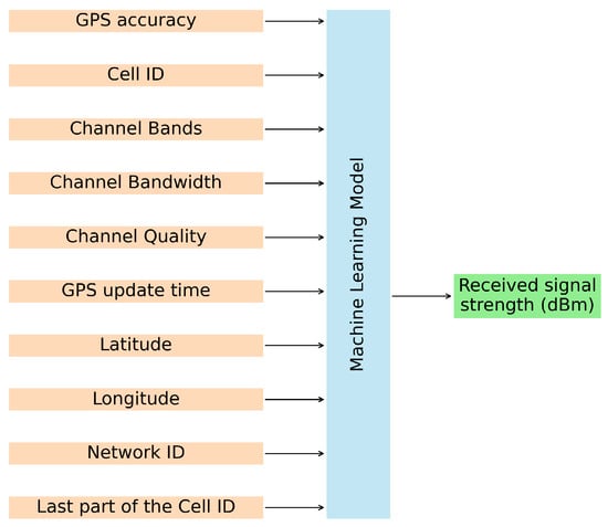
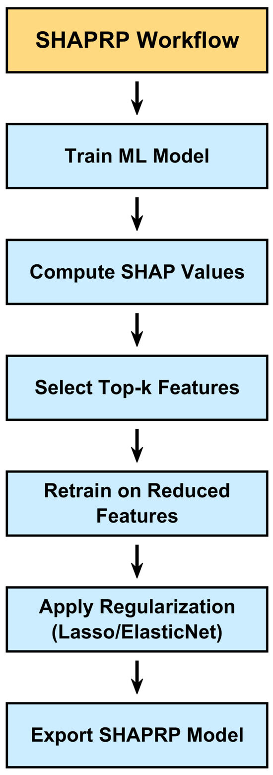
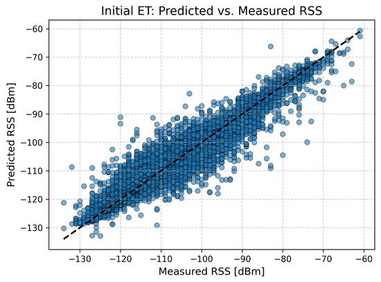
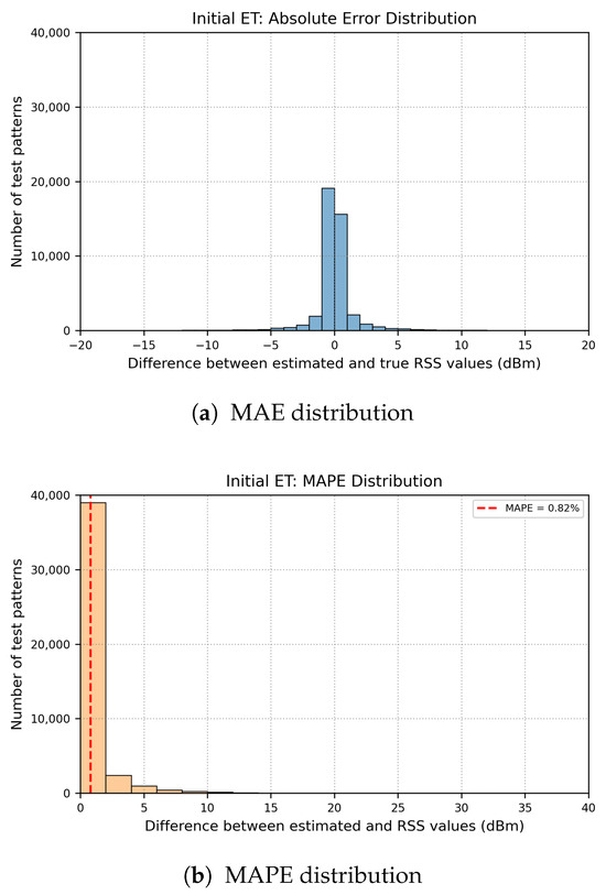
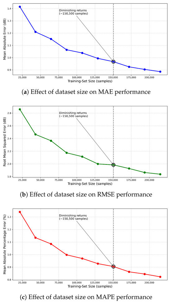
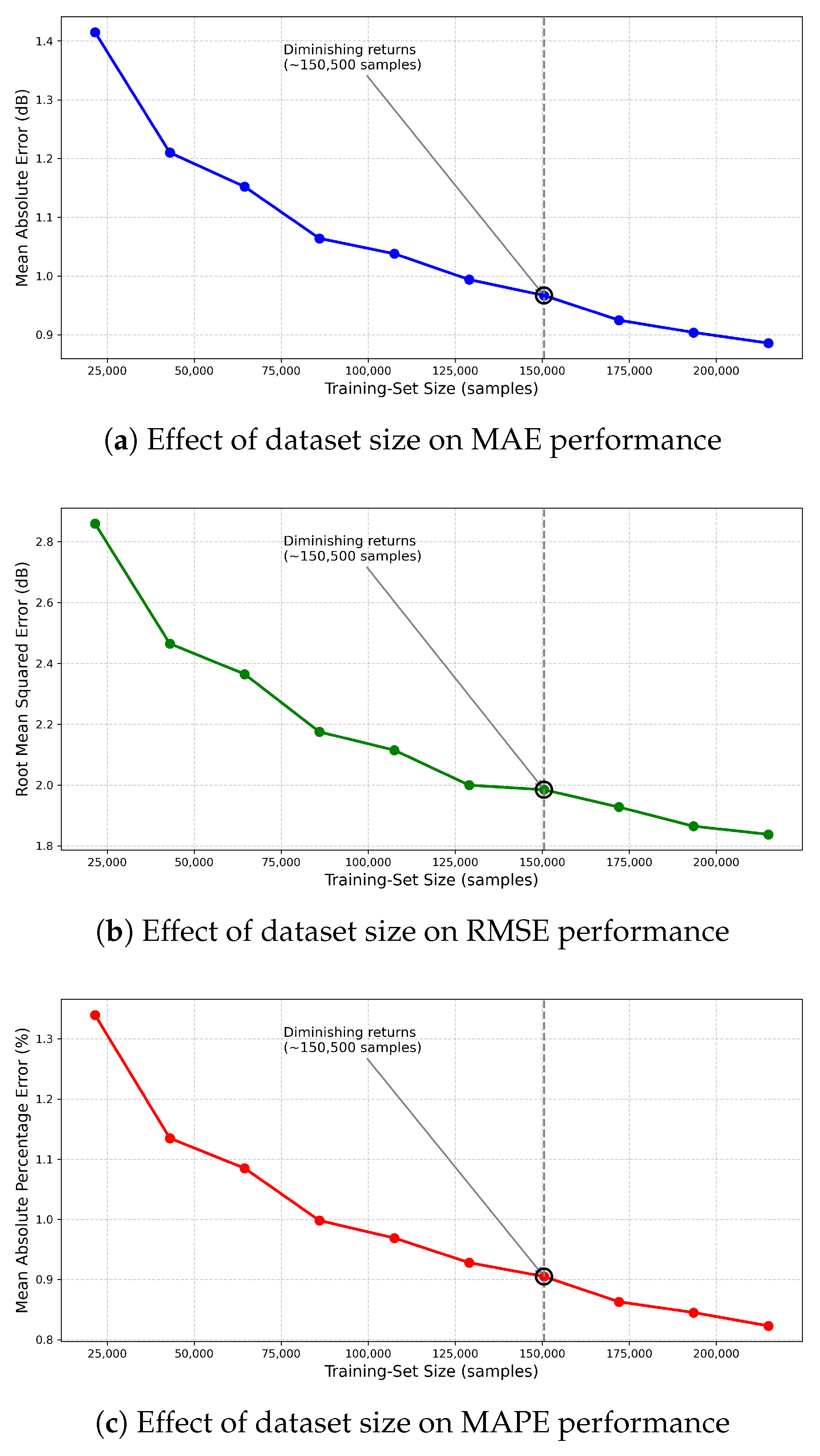
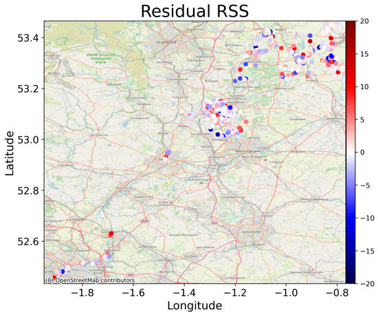
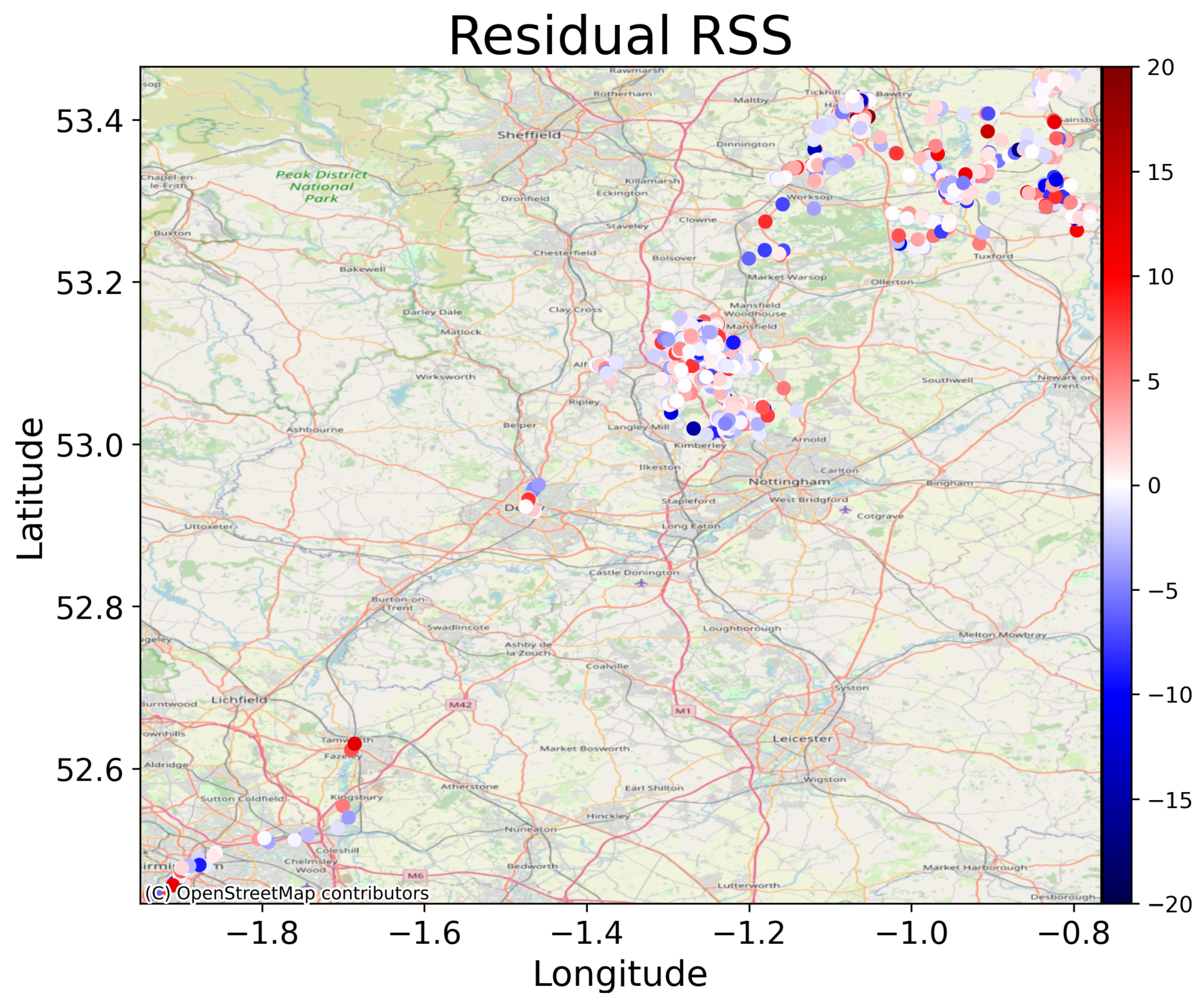
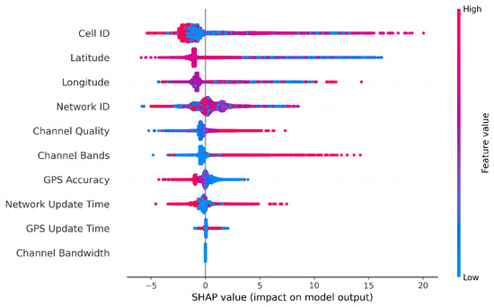
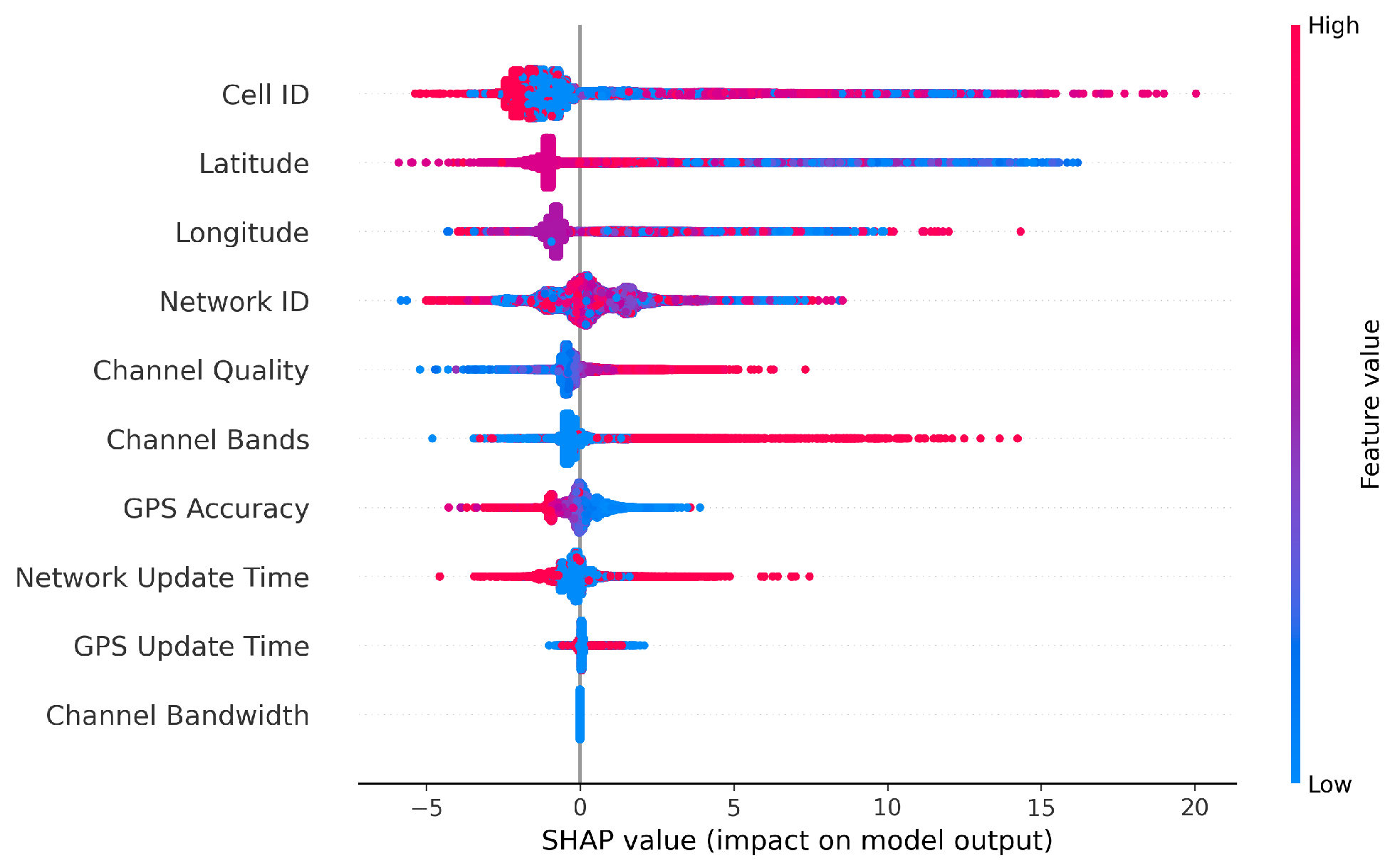
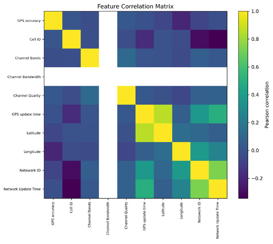
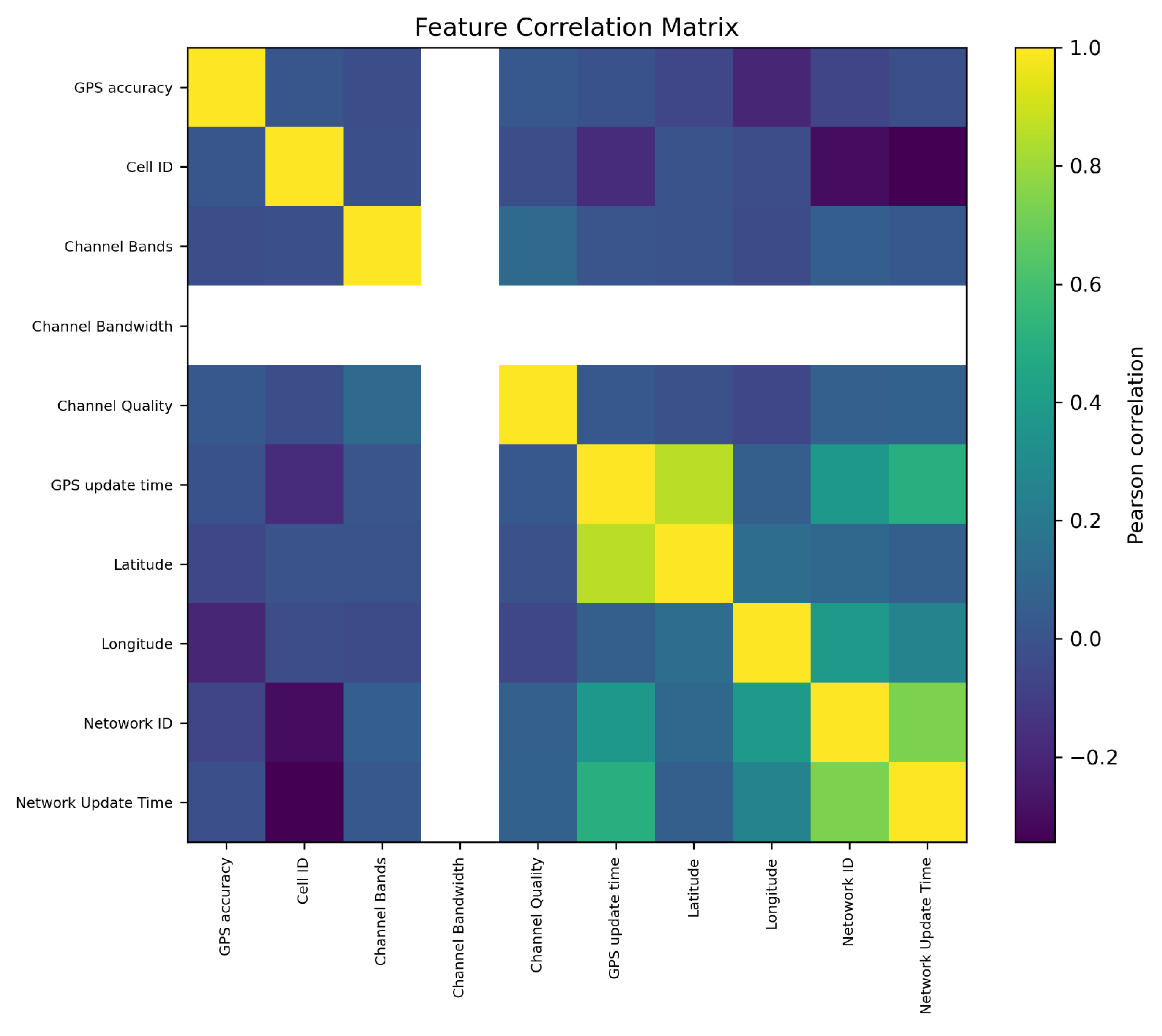
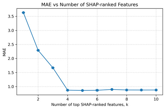
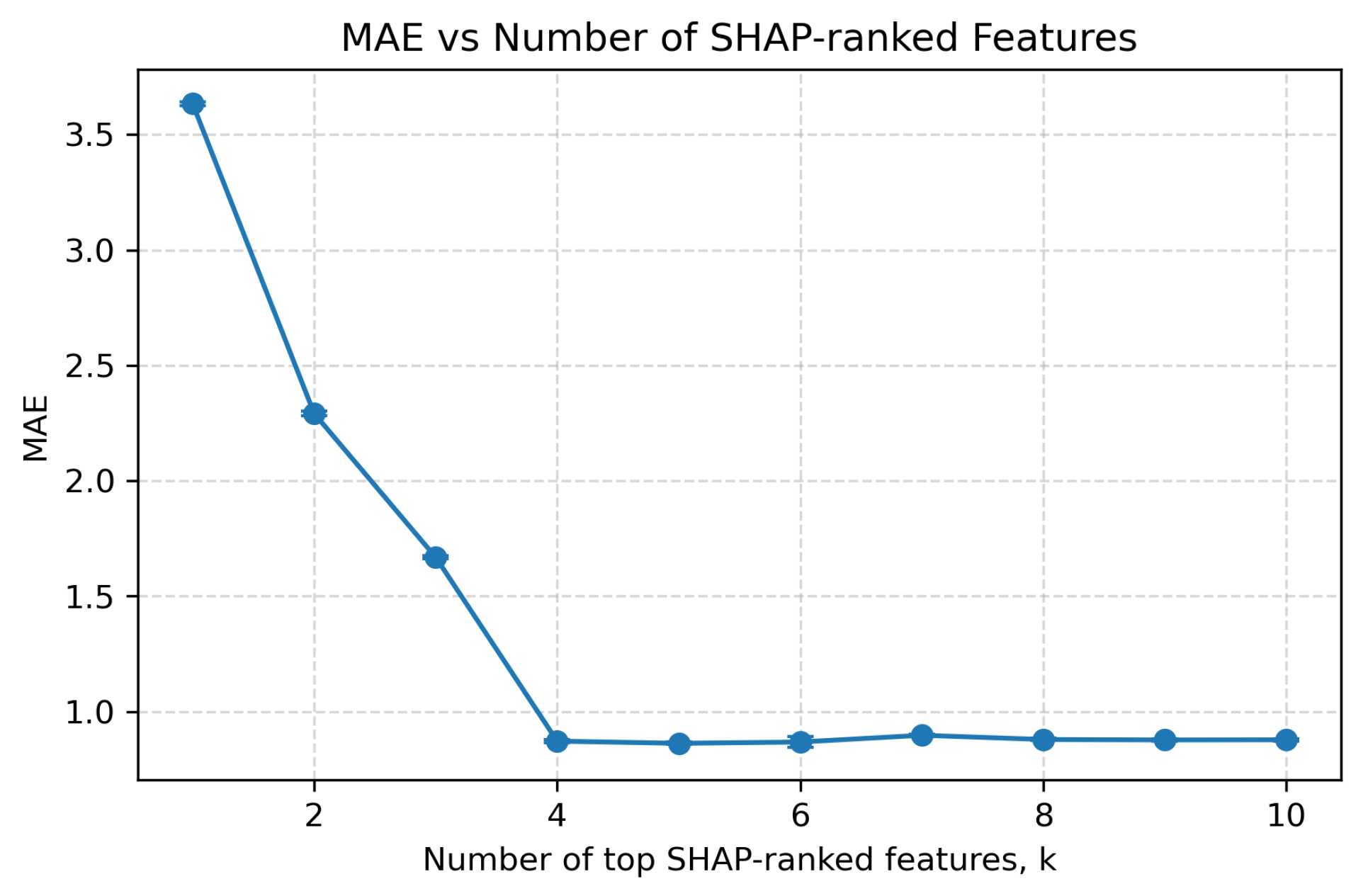
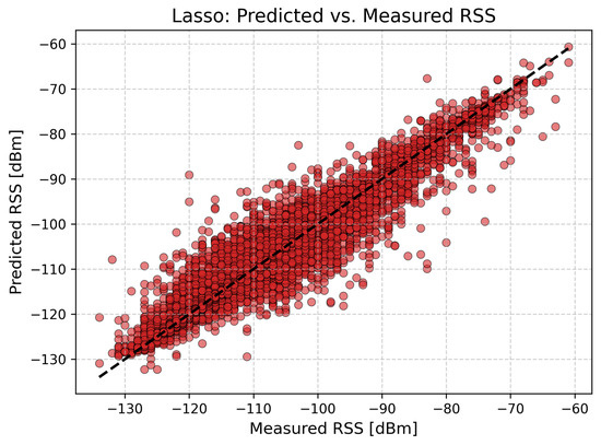
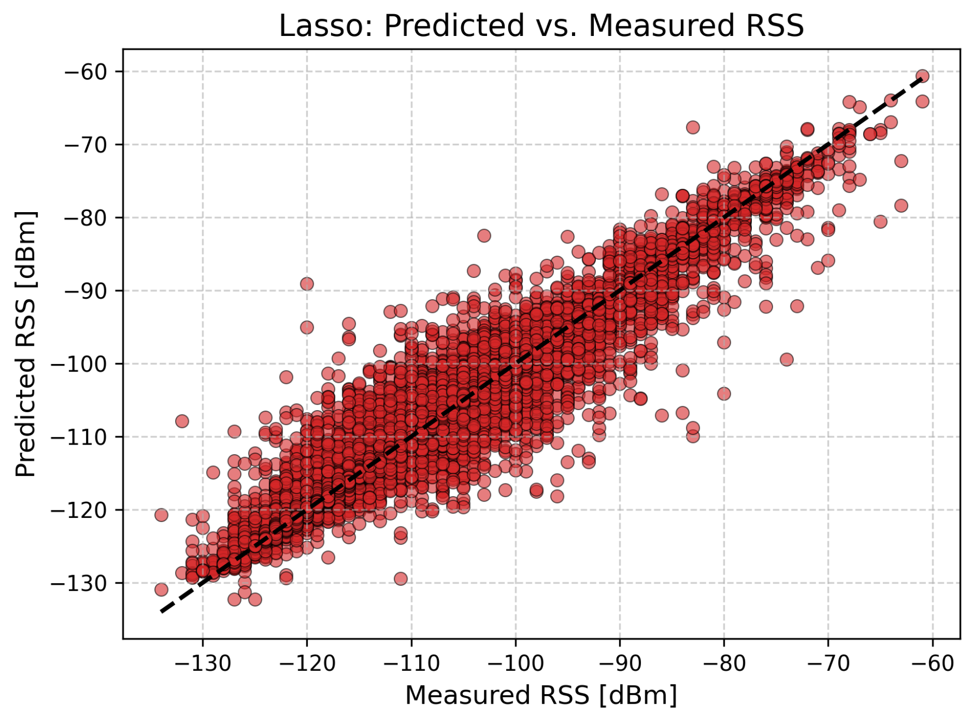
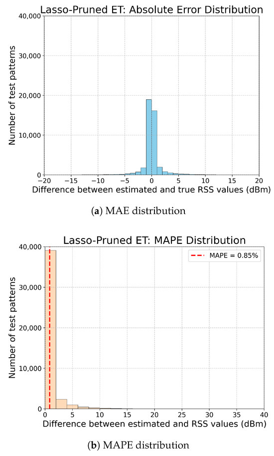
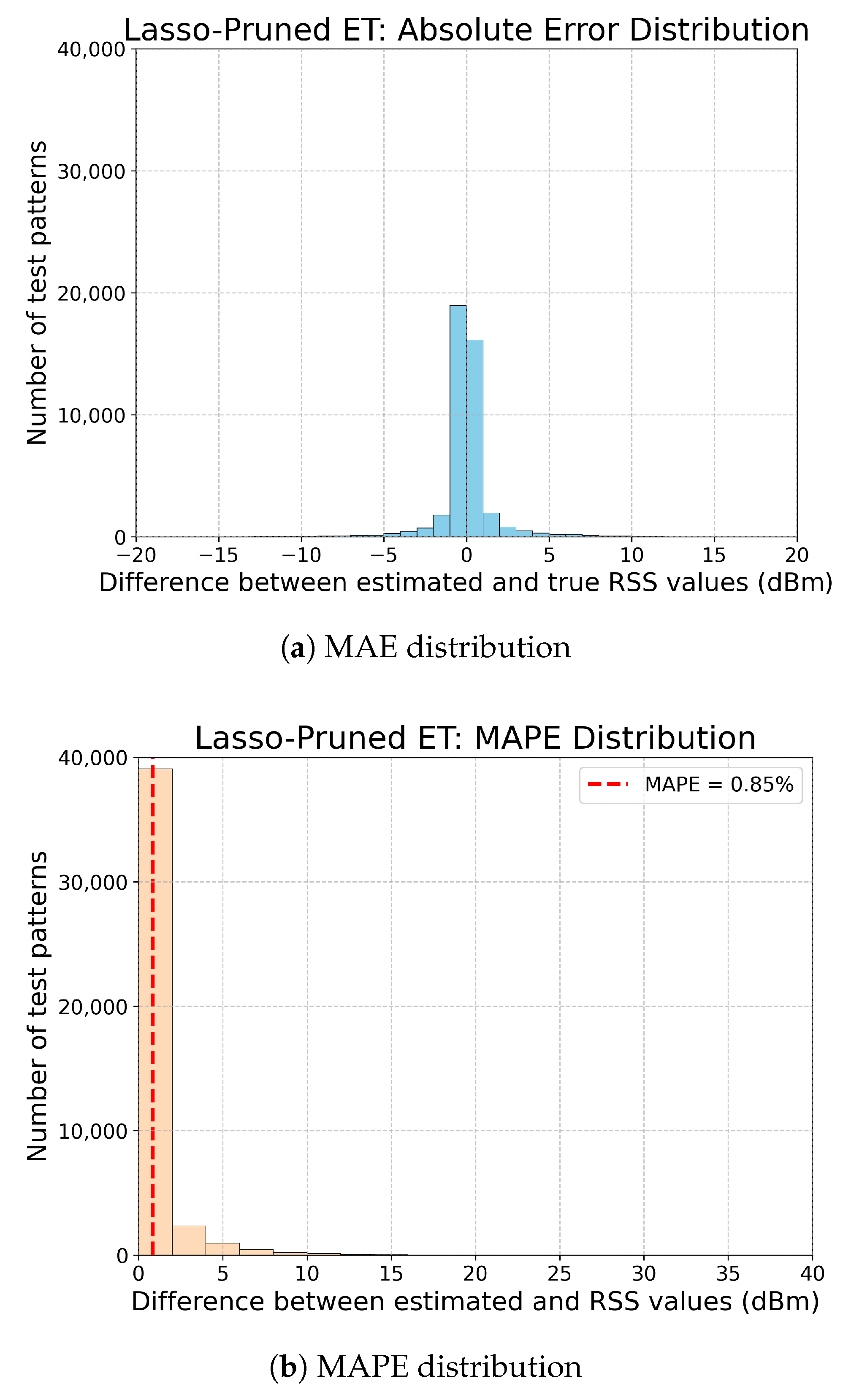
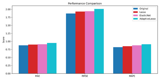
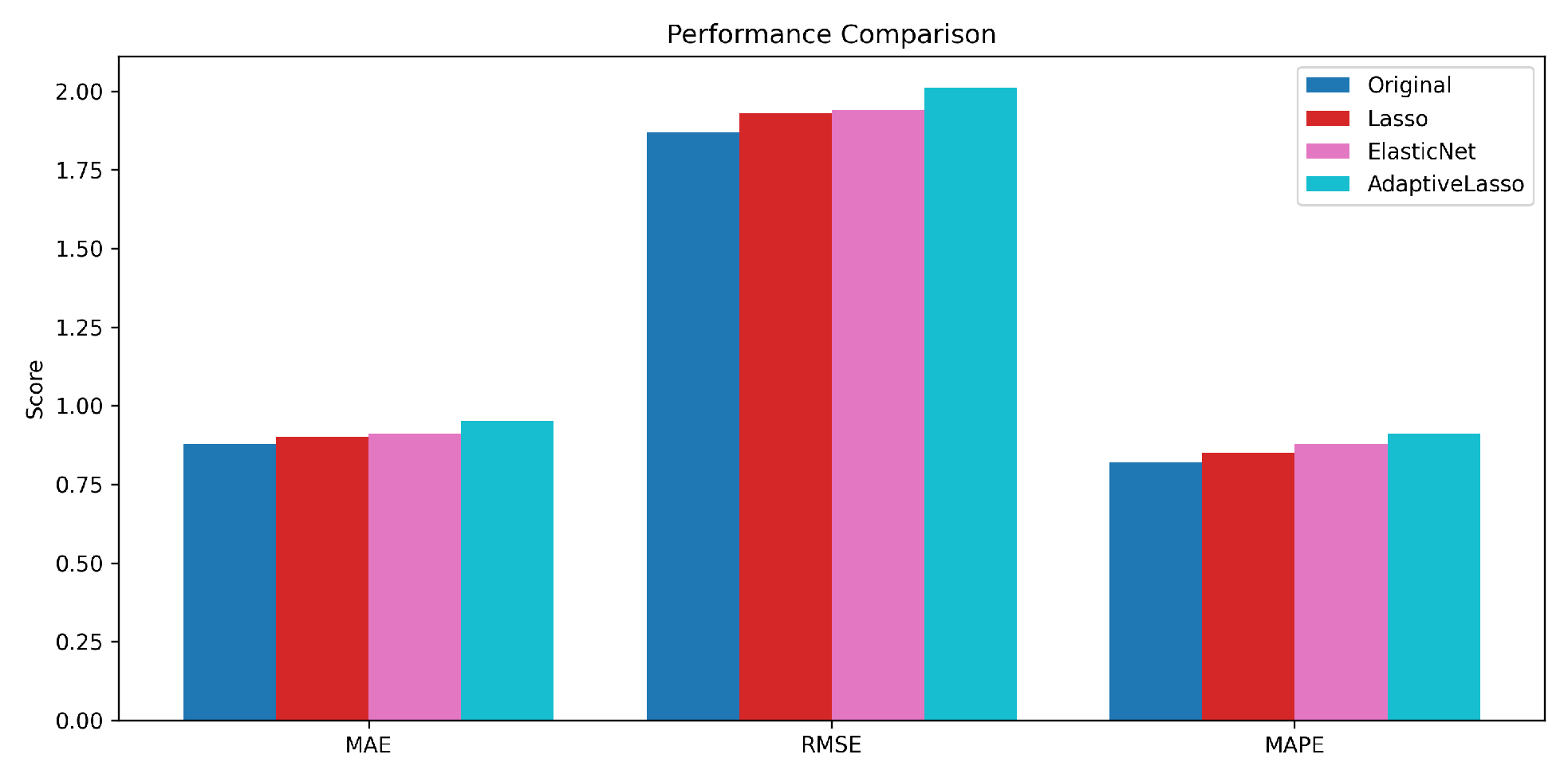
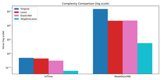
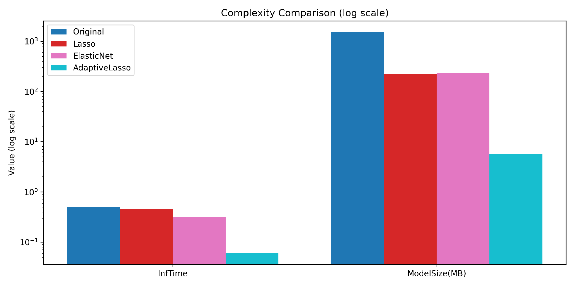

Disclaimer/Publisher’s Note: The statements, opinions and data contained in all publications are solely those of the individual author(s) and contributor(s) and not of MDPI and/or the editor(s). MDPI and/or the editor(s) disclaim responsibility for any injury to people or property resulting from any ideas, methods, instructions or products referred to in the content. |
© 2026 by the authors. Licensee MDPI, Basel, Switzerland. This article is an open access article distributed under the terms and conditions of the Creative Commons Attribution (CC BY) license.