


Abstract
Reliable assessment of shorelines extracted from medium-resolution satellite imagery requires independent high-resolution reference data and statistical methods that account for spatial dependence. This study compared three conventional analyst-assisted shoreline-extraction workflows—histogram thresholding, band ratio, and the Normalised Difference Water Index (NDWI)—at Coronation Park, Lake Ontario, Canada, using Sentinel-2 Level-2A imagery. A manually digitised shoreline derived from a UAV-based orthomosaic acquired approximately 27 h before the Sentinel-2 scene served as the independent reference. The UAV-based reference and each Sentinel-2-derived shoreline were divided into 31 ordered segments. For each Sentinel-2-derived segment midpoint, the shortest planar Euclidean distance to the nearest UAV-based reference midpoint was calculated and used to derive mean absolute error (MAE) and root mean square error (RMSE). Residual spatial autocorrelation was assessed using Moran’s I with 9999 permutations. Because the paired differences departed from normality, the Friedman test was treated as the primary overall comparison, while contiguous spatial-block permutation tests across block sizes of two to eight shoreline locations assessed robustness to local spatial dependence. NDWI achieved the highest positional agreement (MAE = 5.645 m; RMSE = 6.429 m), followed by band ratio (MAE = 14.303 m; RMSE = 14.797 m) and histogram thresholding (MAE = 26.167 m; RMSE = 26.910 m). Significant positive residual spatial autocorrelation was identified for all three methods (Moran’s I = 0.587–0.832, all p < 0.001). The Friedman test confirmed a significant extraction-method effect, χ2(2) = 49.226, p < 0.001, Kendall’s W = 0.794, and the effect remained significant across all tested spatial-block sizes, with empirical p-values ranging from 0.000007 to 0.004630. Among the three conventional methods tested at this large-lake site, NDWI provided the highest positional agreement and therefore offers a defensible baseline for evaluating future Sentinel-2 image-enhancement approaches.
1. Introduction
Shoreline delineation is a fundamental component of coastal and inland-water mapping because the shoreline represents a dynamic interface between land and water. Reliable shoreline information supports erosion and accretion assessment, environmental monitoring, navigation safety, infrastructure planning, coastal-zone management, and climate-change impact analysis [1,2,3,4]. However, a shoreline is not a fixed or universally defined boundary. Its mapped position can vary according to the selected shoreline indicator, water-level conditions, image-acquisition time, sensor resolution, georeferencing accuracy, and extraction method [2,5]. Consequently, reliable shoreline mapping requires both an appropriate delineation technique and validation against an independent, higher-resolution reference dataset [5,6].
Satellite remote sensing provides repeated, spatially consistent, and cost-effective observations over large areas, making it particularly useful for monitoring dynamic marine and inland-water shorelines [1,4,7,8]. Open-access multispectral missions, especially Sentinel-2, provide visible, near-infrared, and shortwave-infrared bands suitable for separating water from non-water surfaces and support thresholding, band-ratio, water-index, and classification-based extraction approaches [6,9,10,11]. Nevertheless, the positional accuracy of Sentinel-2-derived shorelines can be affected by the sensor’s spatial resolution, mixed pixels at the land–water boundary, georeferencing uncertainty, atmospheric and water-surface conditions, turbidity, shadows, wet shoreline materials, and the selected threshold or classification rule [5,6,9,12]. These limitations become particularly important where shoreline features are narrow, irregular, or heterogeneous relative to the image pixel size [5,6,13].
Numerous automated and semi-automated techniques have been developed for shoreline and water-boundary extraction, including single-band thresholding, spectral band ratios, water indices, edge detection, supervised and unsupervised classification, and machine-learning and deep-learning methods [1,3,4,14]. Despite the development of more complex approaches, thresholding, band ratios, and water indices remain widely used because they are interpretable, computationally efficient, reproducible, and applicable to open-access multispectral imagery [6,9,11,12]. Water indices such as the Normalised Difference Water Index (NDWI), Modified Normalised Difference Water Index (MNDWI), and Automated Water Extraction Index (AWEI) were developed to enhance the spectral contrast between water and surrounding surfaces and continue to be applied in water-body and shoreline mapping [4,6,9,15,16,17]. Recent studies nevertheless demonstrate that method performance remains dependent on local shoreline morphology, turbidity, land cover, built-up surfaces, vegetation, sensor resolution, and threshold selection [5,6,9,10,12,18,19,20,21]. No single extraction technique can therefore be assumed to provide the most accurate shoreline under all environmental and image conditions. This study intentionally focuses on histogram thresholding, band ratio, and NDWI rather than attempting an exhaustive comparison of all available shoreline-extraction algorithms. These three workflows represent widely used and conceptually distinct conventional approaches to multispectral land–water separation: scene-specific single-band thresholding, spectral-ratio analysis, and normalised water-index extraction. Their explicit classification rules, limited parameterisation, and reproducible implementation make them suitable for establishing a transparent conventional baseline against an independently derived UAV reference shoreline.
The purpose of the comparison was not to identify a universally superior shoreline-extraction technique, but to select the most defensible method among the three tested workflows for the subsequent Sentinel-2 image-enhancement phase. In that phase, the selected extraction method will be applied consistently to both the original and deep-learning-enhanced imagery. Holding the extraction procedure constant will reduce method-related variation and allow changes in shoreline positional agreement to be evaluated more directly as an effect of image enhancement. Alternative approaches, including MNDWI, AWEI, supervised classification, machine learning, and direct deep-learning shoreline extraction, remain relevant but were outside the predefined scope of this focused baseline-selection study. Their inclusion would change the study into a broader algorithm-benchmarking investigation. Accordingly, the conclusions are restricted to the three tested workflows and do not imply superiority over untested methods.
High-resolution reference data are essential for assessing the positional reliability of shorelines extracted from medium-resolution imagery. UAV photogrammetry has become increasingly important in geomatics and remote sensing because it can provide very-high-resolution imagery at flexible acquisition times and generate detailed orthomosaics, surface models, terrain models, and point clouds [22,23,24,25]. In shoreline applications, UAV orthomosaics can reveal fine-scale land–water and wet–dry boundary features that are blurred or represented by mixed pixels in Sentinel-2 imagery [24,25,26]. UAV and satellite observations are therefore complementary: satellites provide repeated large-area coverage, whereas UAVs provide detailed local observations suitable for interpretation, calibration, and validation [27,28,29]. Previous studies have used aerial imagery, UAV products, and high-resolution orthomosaics to validate satellite-derived shorelines and quantify positional deviations [5,6,11,12].
Despite these advances, several limitations remain relevant. First, shoreline-extraction accuracy is highly context-dependent, and comparative results from marine beaches, tidal coasts, lagoons, or deltaic environments cannot automatically be transferred to large inland lakes [5,6,9,11]. Large-lake shorelines may be influenced by seiche-related water-level changes, local turbidity, heterogeneous natural and artificial shoreline materials, and complex nearshore boundaries [4,7,9,30]. Second, independent UAV validation remains comparatively limited for conventional Sentinel-2 shoreline extraction in large-lake settings. Third, a validated conventional baseline is needed before subsequent image-enhancement approaches can be assessed for genuine positional improvement [6,14,27]. Finally, segment-based shoreline comparisons produce repeated observations along an ordered spatial boundary. Adjacent segment errors may share spatial context and therefore should not automatically be treated as independent observations during statistical comparison.
To address these issues, this study compares three conventional Sentinel-2 shoreline extraction techniques—histogram thresholding, band ratio, and NDWI—at Coronation Park on the northern shore of Lake Ontario, Canada. Sentinel-2 Level-2A imagery was acquired approximately one day after the UAV survey, providing a near-synchronous basis for comparison. The objectives were to: (i) extract shorelines using the three selected Sentinel-2 techniques; (ii) generate an independent high-resolution UAV-derived reference shoreline; (iii) quantify positional agreement using mean absolute error (MAE) and root mean square error (RMSE); (iv) evaluate differences among the methods while accounting for repeated shoreline locations and spatial autocorrelation; and (v) identify the most defensible method among the three tested conventional workflows for use as a fixed shoreline-extraction baseline in subsequent Sentinel-2 image-enhancement research.
The methodological contribution of the study is a near-synchronous UAV–Sentinel-2 validation framework that integrates explicit shoreline-indicator interpretation, GCP-supported UAV reference assessment, repeat reference-shoreline digitisation, water-level comparison, segment-based positional measurement, residual spatial-autocorrelation testing, related-sample method comparison, and contiguous spatial-block robustness testing. Its empirical contribution is a quantitative UAV-validated comparison of three widely used conventional Sentinel-2 shoreline extraction techniques in a heterogeneous large-lake shoreline environment. Its practical contribution is the establishment of a validated conventional baseline against which future Sentinel-2 image-enhancement and deep-learning approaches can be evaluated.
2. Materials and Methods
This study followed a UAV-validated geomatics workflow to compare the positional accuracy of three conventional Sentinel-2 shoreline extraction techniques. The workflow comprised six main stages: (i) selection and preparation of near-synchronous Sentinel-2 and UAV datasets acquired approximately one day apart; (ii) UAV photogrammetric processing, GCP-supported quality assessment, and reference-shoreline digitisation; (iii) Sentinel-2 shoreline extraction using histogram thresholding, band ratio, and NDWI; (iv) division of each shoreline into 31 segments and generation of segment midpoints; (v) calculation of planar nearest-midpoint distances between the Sentinel-2-derived and UAV-reference midpoints, followed by MAE and RMSE computation; and (vi) statistical comparison using residual spatial-autocorrelation testing, Shapiro–Wilk paired-difference checks, the Friedman test, repeated-measures analysis of variance, Holm-adjusted paired comparisons, Wilcoxon sensitivity checks, and contiguous spatial-block permutation testing.
2.1. Study Area
The study area is located along the shoreline of Coronation Park on the northern shore of Lake Ontario, Canada (Figure 1). Lake Ontario is part of the Laurentian Great Lakes system and represents a large inland freshwater environment rather than an open-ocean tidal coast. This distinction is relevant because large-lake shorelines may be affected by seiche-related water-level variation, local wave activity, nearshore turbidity, heterogeneous natural and artificial shoreline materials, and complex land–water boundaries [30].
Figure 1.
Location of the study area at Coronation Park on the northern shore of Lake Ontario, Canada: (a) regional location of the study site within the Lake Ontario coastal environment; and (b) close-up view of the Coronation Park shoreline section used for Sentinel-2 shoreline extraction and UAV-based validation. Base imagery Google Earth (accessed on 1 May 2026).
The analysed shoreline reach was not a uniform open-water boundary. Visual interpretation of the UAV orthomosaic showed a mixture of unconsolidated sand–gravel beach, rocky or riprap-armoured sections, and locally engineered shoreline structures. Terrestrial vegetation occurred landward of parts of the shoreline; however, the analysed reach did not include marsh or vegetated-wetland shoreline. These contrasting surfaces and structures can produce different degrees of spectral mixing at the land–water boundary, particularly where shoreline features are narrower than or comparable to the Sentinel-2 pixel size.
The 31 shoreline segments were generated as ordered analytical units along the continuous study reach for positional comparison. They were not selected, stratified, or balanced as independent replicates of predefined shoreline classes. Accordingly, the reported statistics represent overall method performance across this mixed shoreline reach and do not provide separate accuracy estimates for individual shoreline types.
The UAV survey was conducted on 22 October 2022, while the closest suitable Sentinel-2 Level-2A image was acquired on 23 October 2022. This approximately one-day temporal separation provided a near-synchronous basis for comparison while minimising, but not eliminating, potential differences caused by short-term water-level variation, waves, and nearshore conditions. All horizontal spatial data were stored and analysed in WGS 84/UTM zone 17N (EPSG:32617), with linear measurements expressed in metres.
2.2. Data Sources
Two principal spatial datasets were used: Sentinel-2 Level-2A multispectral imagery and UAV-derived high-resolution imagery. The Sentinel-2 image provided the spectral bands used to extract shorelines through histogram thresholding, band ratio, and NDWI. The UAV imagery was processed into a high-resolution orthomosaic from which an independent reference shoreline was manually digitised.
The UAV images were acquired on 22 October 2022, and the closest suitable Sentinel-2 acquisition was obtained on 23 October 2022 through the Copernicus Browser of the Copernicus Data Space Ecosystem. The Sentinel-2 scene was selected based on temporal proximity to the UAV survey, complete coverage of the study area, and the absence of major cloud cover, cloud shadow, or atmospheric obstruction over the analysed shoreline section.
The principal characteristics, acquisition dates, spatial resolutions, coordinate reference systems, and analytical roles of the Sentinel-2 and UAV datasets are summarised in Table 1. The complete methodological workflow is presented in Figure 2. It includes satellite-band preparation, conventional shoreline extraction, UAV reference-shoreline generation, division of the four shorelines into 31 segments, segment-midpoint generation, planar nearest-midpoint distance calculation, descriptive accuracy assessment, spatial-autocorrelation testing, and repeated and spatially robust statistical comparison.
Table 1.
Characteristics and analytical roles of the spatial datasets used in the study.
Figure 2.
Methodological workflow for the UAV-validated assessment of Sentinel-2 shoreline extraction techniques.
2.2.1. Sentinel-2 Imagery
A Sentinel-2A Level-2A multispectral product acquired on 23 October 2022 was used for shoreline extraction. The product identifier was: S2A_MSIL2A_20221023T161331_N0400_R140_T17TPJ_20221023T215400.SAFE. It was obtained through the Copernicus Browser of the Copernicus Data Space Ecosystem (https://browser.dataspace.copernicus.eu/; accessed on 23 January 2024) and selected as the closest suitable acquisition to the UAV survey conducted on 22 October 2022.
The Level-2A product provides atmospherically corrected bottom-of-atmosphere surface reflectance. The scene was visually inspected to confirm complete coverage of the Coronation Park shoreline section and the absence of major cloud cover, cloud shadow, or obvious atmospheric obstruction over the study area.
The analysis used Band 3 (green), Band 8 (near-infrared), and Band 11 (shortwave infrared). Bands 3 and 8 were used to calculate NDWI and the Green/NIR ratio, whereas Bands 3 and 11 were used for the Green/SWIR ratio. Band 11 was also used independently for histogram thresholding. Bands 3 and 8 have a native spatial resolution of 10 m, while Band 11 has a native spatial resolution of 20 m.
2.2.2. UAV Imagery and Photogrammetric Processing
UAV imagery was acquired on 22 October 2022 using a DJI Matrice 300 RTK platform equipped with a Zenmuse P1 camera (DJI, Shenzhen, China). The survey comprised 504 overlapping images covering the selected Coronation Park shoreline section. The images were processed using ArcGIS Drone2Map version 2023.1.0 and ArcGIS Pro version 3.4 with the Reality Mapping capability (Esri, Redlands, CA, USA) to generate an orthomosaic, digital surface model, digital terrain model, and point cloud. The photogrammetric processing generated more than 3.5 million tie points and approximately 807,000 solution points; these values describe the internal image-matching and reconstruction network and were not interpreted as measures of absolute positional accuracy.
The available ground-control dataset comprised eight ground points surveyed using RTK GNSS and referenced to WGS 1984/UTM Zone 17N (EPSG:32617). The initial ArcGIS Pro Reality Mapping block adjustment was performed without ground-control points. After a positional mismatch was identified, four of the surveyed points were added and manually identified in the relevant overlapping images using the Manage GCPs function. These four points were designated as ground-control points, and the Adjust operation was rerun. The remaining four surveyed points were not used to constrain the refined adjustment. The coordinates, identifiers, and spatial distribution of the four GCPs used in the refined adjustment are provided in the Supplementary File. The final RGB true orthomosaic used for reference-shoreline digitisation was subsequently regenerated from this refined GCP-constrained adjustment.
The available accuracy summary for the complete eight-point RTK GNSS ground-control dataset reported RMSE EN = 0.08 m horizontally and RMSE U = 0.09 m vertically. Because these summary values include points used to constrain the refined adjustment, they are reported as accuracy indicators for the surveyed ground-control dataset rather than as independent checkpoint residuals or as a fully independent estimate of the absolute positional accuracy of the final orthomosaic.
The final RGB true orthomosaic had a ground sampling distance of approximately 0.006 m. This value represents the spatial sampling resolution of the orthomosaic and should not be interpreted as its absolute horizontal positional accuracy. The UAV products were generated in WGS 84/UTM zone 17N (EPSG:32617). Elevation-related products were referenced to the EGM96 geoid model. The high-resolution orthomosaic was subsequently used to interpret and manually digitise the UAV-derived reference shoreline. A detailed description of the UAV image-processing workflow, software settings, image adjustment, tie points, solution points, ground-control checking, and Reality Mapping processing is provided in Supplementary File S1.
2.3. Sentinel-2 Image Pre-Processing
The Sentinel-2 scene was inspected over the Coronation Park shoreline section to confirm that the area of interest was not affected by major cloud cover, cloud shadow, or obvious atmospheric obstruction. Bands 3, 8, and 11 were selected according to their roles in the three shoreline extraction techniques. Bands 3 and 8 were used for NDWI calculation and the Green/NIR ratio, Band 11 was used for histogram thresholding, and Bands 3, 8, and 11 were used for the combined band-ratio analysis described in Section 2.4. All Sentinel-2 bands were handled in WGS 84/UTM zone 17N (EPSG:32617) and clipped to the study-area boundary to reduce the processing extent and maintain spatial consistency with the UAV-derived products. Bands 3 and 8 have native spatial resolutions of 10 m, whereas Band 11 has a native spatial resolution of 20 m.
The initial Band 3/Band 8 calculations therefore used 10 m source data, while the Band 11-based calculations used 20 m source data. No separate standalone resampled raster product was created before shoreline extraction. The archived ArcGIS raster-analysis environment and final classification outputs were examined to clarify the mixed-resolution processing workflow. The archived final classification rasters used for vectorisation had a 20 m cell size for the histogram-thresholding, combined band-ratio, and classified NDWI outputs. Accordingly, the final shoreline vectors compared in this study were generated from binary classification rasters with a 20 m output cell size. The ArcGIS raster-processing environment used nearest-neighbour resampling and a maximum-of-inputs cell-size setting during raster operations. This preserved categorical class boundaries in the binary water–land rasters but also means that the final shoreline positions should be interpreted as outputs of the complete ArcGIS raster-processing workflow rather than as direct representations of the native 10 m or 20 m source-band resolutions alone.
The difference between the native source-band resolutions was therefore retained as an interpretation issue. NDWI originated from two native 10 m bands, histogram thresholding relied on the native 20 m SWIR band, and the combined band-ratio workflow included both 10 m and 20 m source bands. The processing audit confirmed that all three final classified rasters used for vectorisation had a 20 m cell size and that the archived ArcGIS environment used nearest-neighbour resampling and a maximum-of-inputs cell-size setting. However, the exact operation-level snap raster, processing extent, and intermediate grid-alignment sequence could not be reconstructed conclusively for every original raster operation, particularly the sequence by which the 10 m NDWI inputs produced the final 20 m classified raster. No controlled comparison of alternative snap rasters, cell sizes, or resampling methods was performed. Consequently, the reported ranking should be interpreted as a comparison of the three archived end-to-end workflows as implemented, rather than as an experimental isolation of spectral-method effects from raster-resolution and alignment effects.
2.4. Shoreline Extraction Techniques
Three conventional Sentinel-2 shoreline extraction workflows were implemented: histogram thresholding, band ratio, and the NDWI. Each workflow was applied to the same Level-2A scene and study-area extent and ultimately produced a final binary water–land raster, in which water was represented by 1 and non-water by 0. The binary rasters were subsequently converted to polygon features, clipped to the study-area boundary, and converted to shoreline vectors. The boundary associated with the principal Lake Ontario water body was retained, while small disconnected features unrelated to the main shoreline were removed using the same post-processing rule for all three methods. Because threshold selection and artefact removal involved analyst input, these workflows are described as conventional analyst-assisted methods rather than fully automated procedures. The mathematical classification rules used for each method are provided in Section 2.4.1, Section 2.4.2 and Section 2.4.3, and to clarify the threshold values, band combinations, and binary water–land masks applied in the analysis.
2.4.1. Histogram Thresholding
Histogram thresholding was applied to Sentinel-2 Band 11, the shortwave-infrared band, at a 20 m spatial resolution. Water generally exhibits low SWIR reflectance relative to dry land, vegetation, and artificial surfaces. The Band 11 histogram was examined to identify the transition between water and non-water pixel distributions, and scaled bottom-of-atmosphere reflectance values were inspected at representative water and land locations using the ArcGIS inquiry tool.
A scene-specific threshold value of 1150 was selected. Pixels below this value were classified as water, whereas pixels equal to or greater than the threshold were classified as non-water. The binary histogram-thresholding mask was defined as:
where is the Band 11 pixel value at location , = 1 represents water, and = 0 represents non-water. The value of 1150 was selected specifically for the analysed Sentinel-2 scene and was not treated as a universally transferable threshold.
The resulting binary raster was converted to polygons using the ArcGIS Raster to Polygon tool. The output was clipped to the study-area boundary and converted to a line feature representing the land–water class boundary. Disconnected polygons and internal boundaries unrelated to the principal shoreline were excluded before the final histogram-thresholding shoreline was retained for positional analysis.
2.4.2. Band Ratio
The band-ratio technique was applied using Sentinel-2 Band 3 (green), Band 8 (near-infrared), and Band 11 (shortwave infrared). Two spectral ratios were calculated to enhance the contrast between water and non-water surfaces. The Green/NIR ratio was calculated using Equation (2):
The Green/SWIR ratio was calculated using Equation (3):
where , , and are the Sentinel-2 bottom-of-atmosphere reflectance values at location x for the green, near-infrared, and shortwave-infrared bands, respectively. Water tends to produce ratio values greater than 1 because its reflectance decreases substantially from the green band toward the NIR and SWIR regions.
The Green/SWIR ratio combined Band 3 at its native 10 m resolution with Band 11 at its native 20 m resolution. Under the ArcGIS maximum-of-inputs cell-size setting, this mixed-resolution operation was evaluated at a 20 m cell size using nearest-neighbour resampling. No separate standalone resampled version of either source band was created before calculating the ratio.
Each ratio was first classified using a threshold of 1. A pixel was classified as water in the corresponding ratio mask when the ratio value was greater than 1 and as non-water when the ratio value was equal to or below 1. The two binary ratio masks were then combined using a logical union rather than an intersection. The union rule was retained in the primary analysis because it reproduced the originally implemented and archived processing workflow; it was not selected through optimisation against the UAV reference. Because this inclusive rule classifies a pixel as water when either ratio condition is satisfied and may therefore expand the detected water class, a stricter intersection rule was evaluated separately as a diagnostic sensitivity check. The final band-ratio mask was defined in Equation (4) as:
where is the final binary band-ratio mask, is the binary Green/NIR mask, and is the binary Green/SWIR mask. Operationally, the two binary masks were summed in the ArcGIS Raster Calculator, and summed values of either 1 or 2 were reclassified as water. A value of 0 indicated that both ratio tests classified the pixel as non-water. This procedure generated one combined band-ratio mask, corresponding to the single band-ratio shoreline evaluated in the primary statistical dataset.
The archived final combined band-ratio raster used for vectorisation had a 20 m cell size. It was converted to polygons, clipped to the study area, and converted to a shoreline line feature. Small disconnected features and internal boundaries unrelated to the principal lake shoreline were excluded before positional analysis.
2.4.3. Normalised Difference Water Index
NDWI was applied as an index-based water extraction technique. NDWI enhances open-water features by using the spectral contrast between the green and near-infrared bands. NDWI was calculated from Sentinel-2 Band 3 and Band 8 using Equation (5):
where and are the Sentinel-2 green and near-infrared bottom-of-atmosphere reflectance values at location x, respectively. The index enhances water because water generally has higher reflectance in the green band and substantially lower reflectance in the NIR band.
A zero threshold was used to classify the NDWI raster. Pixels with NDWI values greater than 0 were classified as water, whereas pixels with values equal to or below 0 were classified as non-water. The binary NDWI mask was defined as:
The classified water raster was converted to polygons, clipped to the study-area boundary, and converted to a line feature. The boundary of the principal Lake Ontario water body was retained, and disconnected features unrelated to the main shoreline were excluded. The resulting NDWI-derived shoreline constituted the third Sentinel-2 shoreline evaluated against the UAV-derived reference.
2.4.4. Diagnostic Sensitivity Checks
Two diagnostic sensitivity checks were conducted to evaluate the influence of threshold selection and the band-ratio logical-combination rule. These checks were not used to replace the primary 31-segment midpoint-to-midpoint accuracy statistics because their outputs were not manually segmented into the same 31 ordered shoreline units as the main analysis. Instead, they were used to assess the relative behaviour of alternative classification settings under the same study-area and raster-processing environment.
First, Band 11 threshold sensitivity was examined by testing threshold values of 1050, 1100, 1150, 1200, and 1250. Each threshold was applied using the same study-area mask, 20 m output cell size, Band 11 snap raster, and nearest-neighbour raster-processing environment. For each threshold, a cleaned candidate shoreline was generated and compared with the UAV reference using diagnostic UAV-reference midpoint-to-line distances.
Second, the band-ratio logical-combination rule was tested by comparing the original union rule with a stricter intersection rule. Under the union rule, a pixel was classified as water if either the Green/NIR or Green/SWIR ratio condition was satisfied. Under the intersection rule, a pixel was classified as water only if both ratio conditions were satisfied. These diagnostic outputs were compared using UAV-reference midpoint-to-line distances to determine whether the band-ratio shoreline was sensitive to the logical rule used to combine the two ratio masks.
Because both sensitivity checks used diagnostic midpoint-to-line distances rather than the primary Sentinel-derived midpoint-to-UAV-reference midpoint metric, their results are reported separately from the main positional-accuracy table.
2.5. UAV-Derived Reference Shoreline
The UAV-derived RGB true orthomosaic generated using ArcGIS Pro Reality Mapping was used as the independent high-resolution reference dataset for evaluating the three Sentinel-2-derived shorelines. The raster comprised three 8-bit image bands, had a ground sampling distance of 0.006 m, and was referenced to WGS 84/UTM zone 17N. Its natural-colour representation provided detailed visual information on the land–water interface, wet and dry shoreline materials, rocks, vegetation, and other surface features. The reported ground sampling distance represents the spatial resolution of the imagery and should not be interpreted as the absolute horizontal positional accuracy of the UAV product.
The reference shoreline was manually digitised as a polyline from the true orthomosaic. The operational shoreline indicator was defined using the visible wet–dry boundary together with the adjacent land–water interface. Wet sand and other visibly water-affected shoreline surfaces were treated as part of the water-influenced zone because they indicated recent inundation. Accordingly, the digitised shoreline generally followed the transition between dry exposed land and the adjoining wet or water-covered surface rather than being restricted exclusively to the instantaneous visible water edge.
In clearly defined areas, the shoreline was identified from distinct differences in colour, tone, and texture between dry land and the adjacent wet or water-covered surface. Where the boundary was locally ambiguous because of gradual tonal transitions, shallow or turbid water, shadows, or submerged features visible through the water, the shoreline position was interpreted by maintaining the continuity of the dominant wet–dry boundary immediately before and after the ambiguous section. This continuity-based interpretation reduced abrupt and locally implausible changes in the digitised shoreline position.
Isolated underwater features, including submerged rocks, aquatic vegetation, lakebed patterns, and disconnected water patches, were excluded from the principal shoreline unless they coincided with the continuous wet–dry boundary. Small isolated wet areas that were not connected to the main Lake Ontario water body were also excluded. The same interpretation criteria were applied consistently along the full shoreline section.
After digitisation, the reference polyline was visually reviewed and edited to remove unnecessary vertices, isolated artefacts, and local geometric inconsistencies while preserving the selected shoreline indicator. The complete UAV true orthomosaic, the manually digitised reference shoreline, and an example of shoreline interpretation in a complex section are presented in Figure 3. The DSM and DTM were generated as ancillary elevation products during UAV processing but were not used as the primary layers for manually delineating the horizontal shoreline position.
Figure 3.
UAV-derived reference-shoreline delineation: (a) complete RGB true orthomosaic generated using ArcGIS Pro version 3.4 with the Reality Mapping capability (Esri, Redlands, CA, USA); (b) manually digitised UAV-derived reference shoreline overlaid on the true orthomosaic; and (c) enlarged example of shoreline interpretation in a complex section containing wet shoreline materials, shallow water, submerged rocks, and constructed shoreline features. The reference shoreline was delineated using the visible wet–dry boundary and adjacent land–water interface.
To quantify inter-analyst digitisation uncertainty, the UAV reference shoreline was independently redigitised by two additional analysts from the same RGB true orthomosaic using the same shoreline-indicator definition and ambiguity rules. The original UAV-reference segment midpoints were then compared with each repeated digitised shoreline using unsigned planar nearest-midpoint distance measurements. The two independent analyst digitisations produced mean deviations of 0.890 m and 0.409 m, with RMSE values of 1.176 m and 0.560 m, respectively. These values were smaller than the Sentinel-2 shoreline RMSE values for NDWI, band ratio, and histogram thresholding, indicating that manual reference-shoreline interpretation uncertainty was not the dominant source of the observed Sentinel-2 shoreline deviations. Manual interpretation nevertheless remains a residual source of uncertainty.
The UAV imagery was acquired on 22 October 2022 between approximately 09:05 and 09:14 EDT (13:05–13:14 UTC), while the Sentinel-2A scene was acquired on 23 October 2022 at 16:13:31 UTC (12:13:31 EDT), resulting in a temporal separation of approximately 27 h. This near-synchronous acquisition reduced temporal mismatch between the reference and satellite datasets. Nevertheless, short-term water-level variation, local wave conditions, nearshore turbidity, and illumination differences could not be eliminated completely and were considered when interpreting the measured positional deviations. The processing and validation procedures used to generate the true orthomosaic are documented in Supplementary File S1.
To quantify the potential effect of the one-day temporal mismatch, observed water-level records from the Toronto water-level station were examined for 22–23 October 2022. The daily mean water level was 0.219 m on 22 October and 0.223 m on 23 October, giving an absolute daily mean difference of approximately 0.004 m. The observation closest to the Sentinel-2 acquisition time of 2022-10-23 16:13:31 UTC, equivalent to 12:13:31 EDT, was recorded at 12:15 EDT with a water level of 0.200 m. Its corresponding horizontal shoreline displacement and proportion of the measured positional error could not be calculated because contemporaneous local shoreline-slope, wave-setup, run-up, and nearshore hydrodynamic observations were unavailable. Temporal mismatch therefore remains a residual limitation.
2.6. Positional Accuracy Assessment
The positional agreement of the three Sentinel-2-derived shorelines with the UAV-derived reference shoreline was evaluated using a point-based nearest-distance analysis in ArcGIS. Each Sentinel-2-derived shoreline and the UAV-derived reference shoreline was divided into 31-line segments using the Split editing tool. One midpoint was then generated for every segment using the Feature Vertices To Points tool with the point type set to MID. This procedure produced 31 ordered midpoint locations for each of the four shoreline datasets.
The 31-location design produced approximately 10 m alongshore sampling intervals for the three Sentinel-2-derived shorelines, which provided regular coverage of the approximately 310 m analysed reach while retaining sufficient ordered locations for the related-sample statistical analysis. Because the UAV reference shoreline was longer, its corresponding mean interval was approximately 12.4 m. To evaluate whether the results depended on the selected sampling density, each shoreline was additionally dissolved into a continuous polyline and resampled at the centres of 20, 31, 40, and 50 equal along-line intervals. These densities corresponded to approximate Sentinel-2 alongshore intervals of 15.5, 10.0, 7.8, and 6.2 m, respectively. The nearest-midpoint analysis and MAE and RMSE calculations were repeated independently for each sampling density.
For each Sentinel-2-derived midpoint, the Near tool identified the closest midpoint in the UAV-reference dataset and calculated the shortest planar Euclidean distance between the two points. The planar method was used because all datasets were represented in WGS 84/UTM zone 17N (EPSG:32617), with distances expressed in metres. No search radius was specified. The nearest-midpoint approach was selected to provide a consistent and reproducible comparison of the three Sentinel-2-derived shorelines against the same near-synchronous UAV reference shoreline. The metric was intended to quantify unsigned local positional proximity rather than directional shoreline displacement or temporal shoreline-change rates. Applying the same 31-segment framework and ArcGIS Near procedure to all three extraction methods ensured that their relative positional agreement was evaluated using an identical measurement procedure.
The comparison did not enforce a fixed one-to-one match between derived and reference midpoints according to their segment numbers or sequential positions. Instead, every Sentinel-2-derived midpoint was matched independently to the nearest UAV-reference midpoint. The procedure also did not require matches to be unique; consequently, more than one derived midpoint could, in principle, be associated with the same UAV-reference midpoint. Furthermore, distances were not measured along predefined perpendicular transects or constrained to the local shoreline-normal direction. The resulting values therefore represent local nearest-midpoint planar distances rather than signed or strictly perpendicular shoreline displacements.
As a diagnostic check on the nearest-midpoint matching procedure, the number of unique UAV-reference midpoint matches was recorded for each extraction method. The Near analysis produced 25 unique UAV-reference matches for NDWI, 22 for band ratio, and 21 for histogram thresholding. Duplicate matches were therefore present, with the maximum number of derived midpoints matched to the same UAV-reference midpoint being two for NDWI, three for band ratio, and four for histogram thresholding. These diagnostics confirm that the Near analysis provided a nearest-proximity comparison rather than a forced one-to-one correspondence along the shoreline.
This procedure produced 31 distance measurements for each extraction technique and 93 numerical distance values in total. The 31 measurements for each method were retained in their alongshore order during export and subsequent analysis. Although 93 values were generated, they represented three ordered method-specific measurement series across 31 shoreline locations and were therefore not treated as 93 independent observations in the inferential statistical analysis described in Section 2.7.
The Near tool reports non-negative distance magnitudes. These values were used to calculate mean absolute error (MAE) and root mean square error (RMSE). MAE summarised the average magnitude of positional separation between each Sentinel-2-derived shoreline and the UAV reference
MAE was calculated using Equation (7):
where (di) is the planar nearest-midpoint distance at measurement location (i), and (n = 31) is the number of measurements for each extraction technique. Because (di) is already non-negative, the calculated MAE is equivalent to the arithmetic mean of the Near distances.
RMSE was calculated using Equation (8):
RMSE gives greater influence to comparatively large local deviations, whereas MAE describes the average positional separation. Lower MAE and RMSE values indicate closer positional agreement with the UAV-derived reference shoreline. These metrics quantify relative positional agreement with the selected UAV reference and should not be interpreted as absolute geodetic accuracy. Because the measurements were unsigned distance magnitudes, they do not indicate whether a Sentinel-2-derived shoreline was displaced landward or lakeward relative to the reference.
The 31 ordered distance measurements obtained for each extraction technique were subsequently used in the inferential statistical analyses described in Section 2.7. These analyses included Moran’s I testing of residual spatial autocorrelation, the Friedman test, repeated-measures analysis of variance, Holm-adjusted paired comparisons, and contiguous spatial-block permutation testing to assess the robustness of the method effect under repeated shoreline locations and spatial dependence.
2.7. Statistical Analysis
The statistical analysis evaluated whether the positional distances differed among the histogram-thresholding, NDWI, and band-ratio shoreline extraction methods. The analytical dataset contained 31 ordered distance measurements for each method, producing 93 numerical values in total. However, these values were not treated as 93 independent observations. The three methods were evaluated over the same ordered shoreline section, and adjacent segments shared spatial context. Accordingly, shoreline position was incorporated as a repeated or blocking structure, residual spatial dependence was assessed explicitly, and the extraction-method effect was evaluated using complementary non-parametric, parametric, pairwise, and spatial-block procedures.
2.7.1. Spatial-Autocorrelation Assessment
Before comparing the extraction methods, spatial autocorrelation was evaluated in the method-specific residual series using global Moran’s I. For each extraction method, the residual at shoreline location (i) was calculated by subtracting the method-specific mean distance from the observed distance. This is equivalent to obtaining residuals from a model in which extraction method is the only explanatory factor.
Global Moran’s I was calculated as:
where n = 31 is the number of ordered shoreline locations for each method; zi and zj are the mean-centred residuals at locations i and j, respectively; wij is the spatial weight describing the neighbourhood relationship between locations i and j; and S0 is the sum of all spatial weights, defined as:
The spatial-weight matrix was based on first order alongshore adjacency. A weight of wij = 1 was assigned when two segments were immediately adjacent in the ordered shoreline sequence, and wij = 0 otherwise. Consequently, each interior segment was connected to the immediately preceding and following segments, while each end segment was connected to only one neighbouring segment. Self-neighbour relationships were excluded by setting (wii = 0).
Moran’s I was calculated separately for the histogram-thresholding, NDWI, and band-ratio residual series. Positive values indicate that neighbouring shoreline locations tend to have similar residuals, negative values indicate spatial dispersion, and values close to the random expectation indicate limited spatial structure. Statistical significance was assessed using 9999 random permutations of the residual values among the ordered shoreline locations. The empirical permutation p-value was used to test the null hypothesis that the residuals were spatially random.
Significant positive residual spatial autocorrelation was interpreted as evidence that adjacent shoreline measurements were not statistically independent. In that case, the conventional independent-groups one-way ANOVA was considered inappropriate as the principal inferential test, and related-sample and spatial-block procedures were used instead.
2.7.2. Repeated-Measures Comparison
Because each extraction method produced an ordered series of 31 measurements over the same shoreline section, differences among the three methods were assessed using a one-factor repeated-measures analysis of variance. Extraction method was specified as the within-location factor with three levels—histogram thresholding, NDWI, and band ratio—while the ordered shoreline segment position was treated as the repeated or blocking unit.
The null hypothesis was that the mean positional distance was equal across the three extraction methods. The alternative hypothesis was that at least one method had a different mean positional distance. A significance level of (α = 0.05) was adopted. Sphericity was assessed using Mauchly’s test. When the sphericity assumption was violated, Greenhouse–Geisser-adjusted degrees of freedom were reported.
The repeated-measures structure accounted for the dependence among measurements obtained from the same ordered shoreline position and was therefore used as the parametric related-sample comparison instead of an independent-groups one-way ANOVA. Because paired-difference normality could not be assumed for all method comparisons, the repeated-measures ANOVA was interpreted together with the Friedman test, Holm-adjusted paired comparisons, Wilcoxon sensitivity checks, and spatial-block permutation tests described below.
2.7.3. Spatial-Block Permutation Analysis
Because repeated-measures analysis accounts for measurements obtained at the same shoreline locations but does not eliminate residual dependence among neighbouring locations, the robustness of the extraction-method effect was assessed using contiguous spatial-block permutation tests. The ordered shoreline measurements were grouped into blocks so that neighbouring observations remained together during permutation, thereby preserving local alongshore dependence more effectively than unrestricted permutation of individual locations.
Block sizes of two to eight adjacent shoreline locations were examined. Given the approximately 10 m primary sampling interval, this range represented local alongshore dependence scales of approximately 20–80 m. It was selected to evaluate short- to moderate-range spatial dependence while retaining at least four contiguous blocks across the 31-location shoreline sequence; larger blocks would have produced too few blocks for an informative sensitivity assessment. The final shorter block was retained when the number of locations was not exactly divisible by the selected block size.
Within each block, the same permutation of the three extraction-method labels was applied to all locations, thereby preserving the repeated-measures relationship and local dependence structure. Monte Carlo testing with 9999 permutations and a fixed random seed was used for block sizes two and three. Exact enumeration of all blockwise label combinations was used for block sizes four to eight. Consistent significance across this range was interpreted as evidence that the overall method effect was not dependent on one arbitrarily selected block length.
2.7.4. Sensitivity and Pairwise Analyses
A Friedman test was conducted as a non-parametric related-sample test of the overall extraction-method effect. This test used the ordered shoreline positions as blocks and the three extraction methods as related treatments. It provided an overall comparison that did not rely on the parametric distributional assumptions of repeated-measures ANOVA. Before interpreting the pairwise parametric comparisons, Shapiro–Wilk tests were applied to the paired difference scores for each method pair. These tests were used to assess whether the paired differences were consistent with the normality assumption required for paired t-tests. Where normality was not supported, the paired t-test results were interpreted cautiously and were supplemented by Wilcoxon signed-rank tests. When the overall method effect was significant, two-sided paired comparisons were performed between NDWI and band ratio, NDWI and histogram thresholding, and band ratio and histogram thresholding. The paired differences were calculated across the 31 ordered shoreline positions. Holm’s sequential adjustment was applied to the pairwise p-values to control the family-wise error rate. Wilcoxon signed-rank tests were also reported as non-parametric sensitivity checks for the same pairwise comparisons. The inferential hierarchy was therefore: (i) Moran’s I as the spatial diagnostic; (ii) Friedman test as the main non-parametric related-sample comparison; (iii) repeated-measures ANOVA as the supporting parametric related-sample comparison; (iv) Holm-adjusted paired comparisons and Wilcoxon sensitivity checks for method pairs; and (v) contiguous spatial-block permutation tests as the principal spatial-robustness assessment. Overall effect sizes were summarised using Kendall’s W for the Friedman test and partial eta squared (ηp2) for the repeated-measures ANOVA. Pairwise mean differences were reported with 95% confidence intervals and absolute Cohen’s dz values. Statistical significance was defined as p < 0.05, and very small p-values were reported as p < 0.001 rather than p = 0.000.
3. Results
3.1. Positional Accuracy and Alongshore Error Patterns
The positional-accuracy statistics are summarised in Table 2. Accuracy was evaluated using the 31 ordered shoreline segments for each extraction method. Lower MAE and RMSE values indicate closer agreement with the UAV-derived reference shoreline. NDWI produced the lowest shoreline-position error, with an MAE of 5.645 m and an RMSE of 6.429 m. The band-ratio method produced intermediate accuracy, with an MAE of 14.303 m and an RMSE of 14.797 m. Histogram thresholding produced the largest deviations from the UAV reference shoreline, with an MAE of 26.167 m and an RMSE of 26.910 m. The descriptive results therefore show that NDWI provided the closest agreement with the UAV reference shoreline, followed by the band-ratio method, while histogram thresholding showed the weakest positional agreement. The spread of the distance values also differed among the three methods.
Table 2.
Descriptive positional-accuracy statistics for the three Sentinel-2 shoreline extraction methods relative to the UAV-derived reference shoreline.
NDWI showed the smallest standard deviation, indicating more consistent shoreline agreement along the analysed section. Histogram thresholding showed both the highest mean error and the highest standard deviation, indicating that its shoreline position was less stable across the ordered shoreline segments.
The ordered distance profiles further demonstrated that the differences among the methods were not uniform along the shoreline (Figure 4). NDWI generally produced the lowest segment-wise positional deviations, whereas the band-ratio method produced intermediate deviations and histogram thresholding produced the largest deviations across the analysed shoreline sequence. The occurrence of contiguous runs of similar values indicates that neighbouring distance measurements exhibited an ordered spatial pattern rather than behaving as statistically independent observations.
Figure 4.
Segment-wise positional deviations of the histogram-thresholding, NDWI, and band-ratio shorelines from the UAV-derived reference shoreline across 31 ordered shoreline locations. Values represent unsigned planar nearest-midpoint distances. Lower values indicate closer agreement with the UAV-derived reference shoreline.
Overall, the descriptive results consistently ranked NDWI as the method with the highest positional agreement, the band-ratio method as intermediate, and histogram thresholding as the method with the largest positional error.
3.2. Residual Spatial Autocorrelation
Global Moran’s I was used to assess whether the method-specific residuals were spatially random along the ordered shoreline sequence. Significant positive residual spatial autocorrelation was detected for all three extraction methods (Table 3). Moran’s I values were 0.679 for NDWI, 0.587 for the band-ratio method, and 0.832 for histogram thresholding. All three permutation tests returned p < 0.001, indicating that neighbouring shoreline locations tended to have similar residual values. The strongest spatial autocorrelation was observed for histogram thresholding, followed by NDWI and the band-ratio method. These results demonstrate that distance measurements should not be treated as statistically independent observations in a conventional independent-groups one-way ANOVA. The subsequent related-sample and spatial-block analyses were therefore used to evaluate the extraction-method effect while accounting for repeated shoreline locations and residual spatial structure.
Table 3.
Moran’s I results for residual spatial autocorrelation in method-specific shoreline-distance residuals.
3.3. Overall Method Differences and Spatial Robustness
Before interpreting the paired parametric comparisons, the normality of paired difference scores was assessed using Shapiro–Wilk tests. The paired differences departed from normality for all three method pairs: NDWI versus band ratio, W = 0.908, p = 0.0115; NDWI versus histogram thresholding, W = 0.803, p < 0.001; and band ratio versus histogram thresholding, W = 0.906, p = 0.0100. Because the paired differences departed from normality, the Friedman test was treated as the primary overall comparison. It identified a significant extraction-method effect, χ2(2) = 49.226, p < 0.001, with Kendall’s W = 0.794, indicating a large overall effect. The contiguous spatial-block permutation analysis was then used as the principal spatial-robustness assessment. The method effect remained significant for every tested block size from two to eight adjacent shoreline locations, with empirical p-values ranging from 0.000007 to 0.004630. Mauchly’s test indicated that the sphericity assumption was violated, W = 0.455, χ2(2) = 22.832, p < 0.001. Accordingly, the Greenhouse–Geisser-corrected repeated-measures ANOVA was retained only as a supporting parametric comparison and produced the same conclusion, F(1.295, 38.837) = 163.645, p < 0.001, partial ηp2 = 0.845. The concordance of these analyses was interpreted as a robustness check rather than as multiple independent statistical confirmations. The overall related-sample and spatial-robustness results are summarised in Table 4.
Table 4.
Overall related-sample and spatial-block tests for differences among shoreline extraction methods.
3.4. Pairwise Differences Among Extraction Methods
Pairwise comparisons confirmed that all three extraction methods differed significantly from one another (Table 5). The mean paired difference between NDWI and the band-ratio method was −8.658 m, indicating that NDWI produced smaller shoreline deviations than the band-ratio method. The mean paired difference between NDWI and histogram thresholding was −20.522 m, showing a larger advantage for NDWI over histogram thresholding. The band-ratio method also produced significantly smaller deviations than histogram thresholding, with a mean paired difference of −11.864 m. All Holm-adjusted paired comparisons returned p < 0.001. The Wilcoxon signed-rank sensitivity checks also returned p < 0.001 for all method pairs, supporting the same ranking identified by the descriptive statistics and overall related-sample tests: NDWI showed the closest agreement with the UAV-derived reference shoreline, the band-ratio method was intermediate, and histogram thresholding showed the largest deviations.
Table 5.
Holm-adjusted pairwise comparisons among Sentinel-2 shoreline extraction methods using ordered shoreline locations as paired observations.
All three paired comparisons remained significant after Holm adjustment. NDWI therefore produced significantly smaller positional distances than both the band-ratio method and histogram thresholding, while the band-ratio method produced significantly smaller distances than histogram thresholding. This confirms the same ranking shown in the descriptive and overall related-sample analyses: NDWI had the closest agreement with the UAV-derived reference shoreline, the band-ratio method was intermediate, and histogram thresholding had the largest positional deviations.
3.5. Spatial Comparison of the Extracted Shorelines
The spatial overlay of the UAV-derived reference shoreline and the three Sentinel-2-derived shorelines was consistent with the quantitative results (Figure 5). The NDWI-derived shoreline generally followed the UAV reference most closely along the analysed section, although local deviations remained visible. The band-ratio shoreline showed intermediate agreement with the UAV reference, while the histogram-thresholding shoreline exhibited the largest positional departures over much of the shoreline.
Figure 5.
Spatial overlay of the UAV-derived reference shoreline and the three Sentinel-2-derived shorelines extracted using histogram thresholding, NDWI, and the band-ratio method. The overlay illustrates the relative positional agreement of each Sentinel-2-derived shoreline with the UAV reference shoreline.
The spatial comparison also shows that the errors were not distributed randomly along the shoreline. Instead, similar deviations occurred in neighbouring shoreline sections, supporting the significant positive Moran’s I results reported in Section 3.2. This spatial pattern reinforces the need to interpret the method comparison using related-sample and spatial-robustness procedures rather than treating the 31-segment-level distances as independent observations. Overall, the spatial overlay supports the same conclusion as the descriptive and inferential analyses: NDWI provided the closest agreement with the UAV-derived reference shoreline, the band-ratio method showed intermediate agreement, and histogram thresholding showed the weakest positional agreement in this study area.
The mapped shoreline relationships were consistent with the segment-level distance profiles and descriptive statistics. NDWI showed the closest overall visual agreement with the UAV-derived reference shoreline, the band-ratio method showed intermediate agreement, and histogram thresholding showed the largest positional departures. However, the statistical conclusions were based on the measured positional distances and the related-sample and spatially robust analyses rather than on visual interpretation alone.
3.6. Diagnostic Sensitivity and Reference-Uncertainty Checks
The diagnostic threshold-sensitivity test showed that the histogram-thresholding output was sensitive to the selected Band 11 threshold. Using the same study-area mask and raster-processing environment, the tested thresholds produced diagnostic MAE values of 150.576 m for 1050, 27.127 m for 1100, 23.426 m for 1150, 21.130 m for 1200, and 19.680 m for 1250. Although the higher tested thresholds produced lower diagnostic MAE values within this range, these midpoint-to-line results were not used to retrospectively optimise or replace the originally selected threshold because they were not calculated using the primary 31-segment midpoint-to-midpoint assessment framework. These results indicate that the threshold of 1150 used in the main analysis was scene-specific and that histogram thresholding should not be interpreted as a universally transferable shoreline-extraction rule.
The diagnostic band-ratio sensitivity test showed that the logical rule used to combine the Green/NIR and Green/SWIR masks influenced the resulting shoreline. The union rule produced a diagnostic MAE of 5.453 m and RMSE of 8.538 m, whereas the stricter intersection rule produced a diagnostic MAE of 4.197 m and RMSE of 5.732 m. These diagnostic values indicate that the band-ratio method was sensitive to the logical-combination rule, with the intersection rule producing a shoreline closer to the UAV reference under this diagnostic midpoint-to-line comparison.
Reference-shoreline uncertainty was assessed through independent digitisation by two additional analysts. The two independent analyst digitisations produced mean deviations of 0.890 m and 0.409 m from the original UAV-reference shoreline, with RMSE values of 1.176 m and 0.560 m, respectively. These values were smaller than the Sentinel-2 shoreline RMSE values reported in Table 2, indicating that inter-analyst reference-shoreline interpretation uncertainty was not the dominant source of the observed Sentinel-2 shoreline deviations.
Observed water-level records also indicated that the one-day temporal separation between the UAV and Sentinel-2 acquisitions was unlikely to dominate the measured shoreline differences. The daily mean water level was 0.219 m on 22 October 2022 and 0.223 m on 23 October 2022, giving an absolute daily mean difference of approximately 0.004 m. The observation closest to the Sentinel-2 acquisition time was 0.200 m at 12:15 EDT on 23 October 2022. Because contemporaneous local shoreline-slope, wave-setup, and nearshore hydrodynamic observations were unavailable, the corresponding horizontal shoreline displacement and its proportion of the measured positional error could not be calculated. Temporal mismatch therefore remains a residual limitation.
The sampling-density sensitivity analysis showed that the relative ranking of the three extraction methods was unchanged when 20, 31, 40, or 50 equally spaced locations were used. Across the tested densities, NDWI produced MAE values of 5.107–7.197 m and RMSE values of 5.937–7.889 m. The band-ratio method produced MAE values of 13.877–15.112 m and RMSE values of 14.452–15.443 m, while histogram thresholding produced MAE values of 25.401–26.883 m and RMSE values of 26.292–27.574 m. The absolute error estimates therefore varied with sampling interval, particularly at the coarsest density, but NDWI remained first, band ratio second, and histogram thresholding third at every tested density as shown in Table 6.
Table 6.
Sampling-density sensitivity of nearest-midpoint positional errors.
4. Discussion
This study demonstrates that the selected Sentinel-2 shoreline extraction method materially affected the position of the derived shoreline at Coronation Park. NDWI produced the closest agreement with the UAV-derived reference shoreline, the band-ratio method showed intermediate agreement, and histogram thresholding produced the largest positional deviations. These differences were evident in the MAE and RMSE values, the alongshore distance profiles, the pairwise comparisons, and the spatial overlay of the extracted shorelines. All three pairwise comparisons remained significant after Holm adjustment, and the overall method effect remained significant after accounting for repeated shoreline locations, non-normal paired differences, and residual spatial autocorrelation. The results therefore support NDWI as the most defensible conventional benchmark among the three tested workflows for this site, while not implying that NDWI will necessarily be the best-performing method in every shoreline environment.
4.1. Comparative Performance of the Shoreline Extraction Methods
NDWI achieved the lowest positional error, with an MAE of 5.645 m and an RMSE of 6.429 m. Its stronger performance is consistent with the normalised green–NIR contrast used by the index. Water generally retains comparatively greater green-band reflectance while strongly absorbing near-infrared energy, whereas many adjacent land surfaces exhibit greater near-infrared reflectance; this contrast enhanced the land–water transition without relying on a scene-specific absolute reflectance threshold [15]. In the present study, this contrast appears to have provided a comparatively stable representation of the land–water transition across the heterogeneous shoreline, which contained wet beach materials, rocks, vegetation, artificial structures, and shallow nearshore water. Previous research has similarly shown that water-index performance can be strong where open water is spectrally distinct from surrounding land, although the resulting accuracy remains dependent on turbidity, mixed pixels, land cover, shoreline morphology, sensor resolution, and threshold selection [18,19,31].
The relatively low NDWI errors should nevertheless be interpreted carefully. An RMSE of 6.429 m does not imply that Sentinel-2 resolved shoreline features at a true spatial resolution of 6.429 m or that the resulting shoreline had equivalent absolute geodetic accuracy. A vector boundary extracted from a classified raster can exhibit an average positional separation smaller than the nominal pixel dimension when compared with a reference line, particularly where the raster boundary follows a consistent cell-edge pattern. The reported value therefore represents agreement with the selected UAV-derived reference under the adopted extraction and distance-measurement procedures, rather than the intrinsic resolving capability of the sensor.
The spatial-resolution issue also requires explicit consideration. Bands 3 and 8 have native resolutions of 10 m, whereas Band 11 has a native resolution of 20 m. However, inspection of the archived classified rasters used for vectorisation showed that the final histogram-thresholding, combined band-ratio, and NDWI outputs all had a 20 m cell size. The observed advantage of NDWI therefore cannot be attributed simply to its final shoreline having been generated from a finer 10 m output raster. The initial NDWI calculation nevertheless originated from two native 10 m bands, while the histogram-thresholding workflow relied on the native 20 m SWIR band and the combined band-ratio workflow included both 10 m and 20 m source bands. The internal alignment or resampling conducted during the ArcGIS raster operations may therefore have contributed to boundary placement, but the archived workflow does not provide sufficient evidence to isolate or quantify that contribution. The performance difference should consequently be interpreted as the combined outcome of spectral formulation, thresholding behaviour, source-band resolution, raster processing, and local shoreline characteristics rather than as the effect of one factor alone.
Histogram thresholding produced the weakest positional agreement among the three tested methods, with an MAE of 26.167 m and an RMSE of 26.910 m in the primary 31-segment analysis. The method benefits from conceptual simplicity and transparent implementation, but its performance depends directly on the selected threshold value. The value of 1150 was derived for the analysed Sentinel-2 scene and should not be treated as a transferable threshold for other dates, sensors, or shoreline environments. The diagnostic threshold-sensitivity test confirmed this limitation: tested Band 11 thresholds from 1050 to 1250 produced diagnostic MAE values ranging from 150.576 m to 19.680 m. Although these diagnostic midpoint-to-line values are not directly equivalent to the primary 31-segment midpoint-to-midpoint accuracy statistics, they show that fixed-threshold shoreline extraction is highly sensitive to local spectral conditions. Wet sediment, shallow water, shadows, submerged material, vegetation, and mixed land–water pixels may all produce reflectance values that overlap the selected water and non-water classes. These factors help explain why histogram thresholding produced the largest positional deviations in this study [9,11,12,18]. An automatic thresholding procedure such as Otsu was not included; therefore, the sensitivity analysis quantifies the influence of alternative manually specified thresholds but does not compare manual and automatic threshold selection.
The band-ratio method showed intermediate positional agreement, with an MAE of 14.303 m and an RMSE of 14.797 m. This indicates that combining Green/NIR and Green/SWIR information can support shoreline discrimination, but the result remains sensitive to the logical structure of the classification rule. In the main analysis, the two ratio masks were combined using a union rule, whereby a pixel was classified as water if either the Green/NIR or Green/SWIR condition was satisfied. Because either condition was sufficient, marginal or mixed shoreline pixels classified as water by only one ratio mask were retained in the combined water class, which may have extended the extracted boundary relative to the more restrictive intersection rule. The diagnostic sensitivity check showed that using a stricter intersection rule produced a different shoreline and lower diagnostic midpoint-to-line error. This indicates that the band-ratio result was influenced not only by the selected spectral bands but also by the rule used to combine the binary masks.
The comparative findings reinforce the broader conclusion that no single conventional extraction method should be assumed to perform uniformly across sites. Method performance is influenced by the interaction of spectral bands, threshold rules, pixel size, water clarity, shoreline materials, vegetation, artificial structures, and the operational definition of the shoreline [6,18,20,21]. The present ranking is therefore a site-specific empirical finding for the Coronation Park scene and processing workflow. Its value lies in establishing a validated local benchmark rather than proposing NDWI as a universally optimal solution.
4.2. Spatial Dependence and Robustness of the Method Comparison
Significant positive residual spatial autocorrelation was detected for all three shoreline-extraction methods, confirming that errors at neighbouring shoreline locations were spatially structured rather than independently distributed. Histogram thresholding produced the strongest autocorrelation (Moran’s ), followed by NDWI () and band ratio (); all three results were significant at . The comparatively strong clustering associated with histogram thresholding plausibly reflects the application of one absolute SWIR threshold across contiguous shoreline reaches. Adjacent locations with similar shallow-water conditions, substrate characteristics, mixed land–water pixels, or engineered shoreline features may therefore experience sustained over- or under-classification, producing consecutive residuals of similar magnitude. NDWI’s normalised green–NIR contrast reduced the overall positional error but did not eliminate spatially coherent effects associated with neighbouring mixed pixels and common shoreline morphology. The lower Moran’s observed for the band-ratio workflow may indicate greater local variability in the responses of its two ratio conditions and their logical-union combination. These explanations are offered as plausible process-based interpretations; the present study did not conduct a feature-stratified causal analysis of individual shoreline types.
The presence of residual spatial autocorrelation demonstrates why the ordered shoreline measurements should not be treated as fully independent observations. A conventional independent-groups one-way ANOVA would ignore both the repeated evaluation of the same shoreline locations and the spatial similarity among neighbouring locations, potentially overstating the effective amount of independent information. The statistical analyses were therefore assigned distinct roles. Because the paired difference scores departed from normality, the Friedman test was treated as the primary overall related-sample comparison. It identified a significant extraction-method effect, , , with Kendall’s , indicating a large overall effect.
The contiguous spatial-block permutation analysis was used as the principal spatial-robustness assessment. The extraction-method effect remained significant across block sizes of two to eight adjacent shoreline locations, representing approximate alongshore dependence scales of 20–80 m, with empirical -values ranging from 0.000007 to 0.004630. This result shows that the comparative method effect was not dependent on a single arbitrarily selected block size. The Greenhouse–Geisser-corrected repeated-measures ANOVA was retained only as a supporting parametric comparison and produced the same conclusion, , and partial . The agreement among these analyses should therefore be interpreted as a robustness check under different assumptions rather than as multiple independent confirmations of the same result.
Overall, the statistical evidence supports a stable ranking of NDWI, band ratio, and histogram thresholding across the ordered shoreline locations, non-normal paired differences, residual spatial autocorrelation, and alternative spatial-block lengths. NDWI consequently provides the strongest conventional baseline among the three tested workflows for this study area. The findings also demonstrate that future segment-based shoreline-validation studies should explicitly account for the repeated and spatially ordered nature of shoreline measurements rather than analysing them as independent observations.
4.3. UAV-Based Validation and Interpretation of Positional Agreement
The UAV-derived RGB true orthomosaic was a central strength of the study. Its 0.006 m ground sampling distance provided substantially greater visual detail than the Sentinel-2 imagery and allowed the reference shoreline to be interpreted from colour, tone, texture, wet and dry materials, shallow water, rocks, and constructed shoreline features. The UAV dataset was supported by eight RTK GNSS-surveyed ground points. Four points were used as GCPs in the refined adjustment, while the remaining four were not used to constrain it. The reported RMSE EN = 0.08 m and RMSE U = 0.09 m summarise the complete eight-point ground-control dataset and should not be interpreted as independent checkpoint residuals or as a fully independent estimate of the absolute positional accuracy of the final orthomosaic. The UAV survey was acquired approximately 27 h before the Sentinel-2 scene, reducing temporal mismatch compared with reference data collected weeks, months, or years apart. This approach is consistent with previous studies emphasising the value of high-resolution aerial or UAV-derived products for validating satellite shorelines [5,6,11,12,30].
The UAV product should nevertheless be regarded as an independent high-resolution reference rather than error-free ground truth. The reported 0.006 m value is the raster ground sampling distance, not the absolute horizontal accuracy of the digitised shoreline. The shoreline was manually interpreted using an operational wet–dry and adjacent land–water indicator. In ambiguous areas, continuity of the dominant boundary was used, while isolated submerged features and disconnected wet areas were excluded. These procedures improved consistency, but they necessarily involved analyst judgement. The repeat inter-analyst digitisation check showed mean deviations of 0.890 m and 0.409 m, with RMSE values of 1.176 m and 0.560 m, respectively, relative to the original UAV-reference shoreline. These values were smaller than the Sentinel-2 shoreline RMSE values, indicating that manual reference interpretation uncertainty was not the dominant source of the observed Sentinel-2 deviations. Alternative shoreline indicators, such as the instantaneous water edge, a fixed elevation contour, or a vegetation line, could nevertheless produce a different reference position. The UAV reference followed the visible wet–dry transition and included visibly wet sand within the water-influenced zone, whereas the Sentinel-2 spectral boundary may occur closer to the instantaneous water edge. This indicator mismatch may have introduced a systematic offset common to all three methods and contributed to their absolute MAE and RMSE values. Because the wet-sand-zone width was not measured and varied across the heterogeneous shoreline reach, no numerical correction was applied.
The approximately one-day acquisition separation also reduced but did not eliminate temporal uncertainty. The water-level comparison indicated that the daily mean water level differed by only approximately 0.004 m between the UAV acquisition date and the Sentinel-2 acquisition date, and the observation closest to the Sentinel-2 acquisition time was 0.200 m. This difference is negligible relative to the Sentinel-2 pixel size and the measured shoreline deviations. Therefore, water-level mismatch is unlikely to explain the observed differences among the extraction methods. Nevertheless, the acquisitions were not simultaneous, and short-term effects such as local waves, seiche-related variability, nearshore turbidity, illumination differences, or wet-surface persistence may still have contributed to local deviations.
The positional metric must also be interpreted according to the geometry of the Near analysis. Each Sentinel-2 derived midpoint was matched independently to the nearest UAV-reference midpoint. Sequential segment correspondence was not enforced, matches were not required to be unique, and distances were not constrained to perpendicular shoreline-normal transects. The resulting MAE and RMSE therefore quantify unsigned nearest-midpoint proximity. They do not indicate whether a shoreline was displaced landward or lakeward, and they should not be interpreted as signed shoreline-change measurements. In curved or irregular sections, a nearest-midpoint distance may also be shorter than a displacement measured along a fixed normal transect. The metrics are appropriate for comparing relative positional agreement among the three methods under a common procedure, but they do not capture every geometric aspect of shoreline displacement.
The sampling-density sensitivity analysis demonstrated that the comparative ranking was robust across the tested intervals, but it did not remove the geometric limitations of the nearest-midpoint metric. Absolute MAE and RMSE values changed with sampling density, and curved or turning sections may allow a derived midpoint to match a nearby but non-corresponding reference midpoint. Consequently, the analysis supports comparative positional-proximity assessment but not signed landward/lakeward displacement or shoreline-normal change measurement.
4.4. Methodological and Practical Implications
The study makes an empirical, methodological, and practical contribution. Empirically, it provides a UAV-validated comparison of three widely used conventional Sentinel-2 extraction workflows in a heterogeneous large-lake setting. The results extend shoreline-validation evidence beyond the marine beaches, tidal coasts, lagoons, and deltaic environments that dominate much of the literature. Lake Ontario presents a different combination of water-level behaviour, turbidity, natural shoreline materials, artificial structures, vegetation, and nearshore spectral complexity. The results show that these local conditions can produce substantial differences among otherwise simple and commonly used extraction methods.
Methodologically, the study integrates an explicit shoreline-indicator definition, near-synchronous UAV validation, ordered segment-level positional measurements, spatial-autocorrelation testing, related-sample comparison, pairwise sensitivity checks, and contiguous spatial-block permutation analysis. The statistical component is particularly important because it demonstrates that spatial dependence can be substantial even over a relatively short shoreline section. Future comparative shoreline studies should therefore examine the spatial structure and distributional assumptions of their error measurements rather than assuming that adjacent samples provide independent information.
Practically, the study establishes a UAV-validated conventional reference point for the next stage of Sentinel-2 image-enhancement research. NDWI provides the strongest baseline among the three tested workflows because it produced the lowest MAE and RMSE, showed the closest visual agreement with the UAV-derived reference shoreline, and remained the strongest method after related-sample and spatially robust statistical testing. An enhanced or deep-learning-based method should therefore not be considered successful merely because it creates a visually sharper image. It should demonstrate a lower positional error than the validated NDWI baseline under the same shoreline definition, reference dataset, spatial sampling design, and statistical framework.
This benchmark should remain explicitly local. The reported NDWI accuracy should not be transferred directly to other lakes, seasons, sensors, or shoreline types. Operational adoption should be preceded by local validation, particularly where water clarity, bottom visibility, vegetation, wet sediment, artificial structures, or shoreline slope differ from the present site. Previous research has similarly shown that shoreline and water-extraction performance is context-dependent [2,9,16,17].
4.5. Limitations and Future Work
Several limitations should be acknowledged. First, the analysis was based on a single large-lake shoreline section and one near-synchronous UAV–Sentinel-2 image pair. The results therefore provide a site-specific empirical comparison for the Coronation Park shoreline rather than a universal ranking of Sentinel-2 shoreline extraction methods. Although the analysed reach included sand–gravel, rocky or riprap-armoured, and engineered shoreline sections, it did not include marsh or vegetated-wetland shoreline, and the 31 segments were not stratified by shoreline type. The results should therefore not be interpreted as shoreline-class-specific performance estimates or transferred directly to shoreline environments not represented in the present dataset. Method performance may differ across other shoreline types, seasons, water-level conditions, turbidity levels, vegetation densities, substrate materials, atmospheric conditions, and sensor-acquisition geometries. Future studies should apply the same UAV-validated workflow across multiple large-lake, coastal, estuarine, and engineered shoreline environments to test whether the relative ranking of NDWI, band ratio, and histogram thresholding remains stable. The comparison was intentionally limited to three conventional shoreline-extraction workflows and should not be interpreted as an exhaustive benchmark of all available methods. NDWI was selected only as the most accurate of the three tested workflows for use as a fixed extraction procedure in the subsequent image-enhancement phase. Future studies could extend the same UAV-validated framework to MNDWI, AWEI, classification-based, and machine-learning approaches.
Second, although observed water-level records were used to characterise the approximately 27 h temporal mismatch, the UAV and Sentinel-2 acquisitions were not simultaneous. The observed daily mean water-level difference was approximately 0.004 m. Its corresponding horizontal shoreline displacement and proportion of the measured positional error could not be calculated because contemporaneous local shoreline-slope, wave-setup, run-up, and nearshore hydrodynamic observations were unavailable. Additional temporal influences, including turbidity, illumination, wind- or seiche-related nearshore effects, and wet-surface persistence, were not incorporated into the positional-error model. Future studies should, where feasible, coordinate UAV and satellite acquisition more closely and collect co-located shoreline-slope, hydrodynamic, and nearshore-condition observations to separate extraction-method error from short-term environmental variability.
Third, the UAV reference shoreline was manually interpreted from the RGB true orthomosaic. Although the operational shoreline indicator, ambiguity rules, GCP-supported processing information, and inter-analyst digitisation assessment strengthened the reference dataset, manual interpretation remains a residual source of uncertainty. The two independent analyst digitisations quantified variability under the same shoreline-indicator definition, but alternative indicators—such as the instantaneous water edge, a fixed elevation contour, or a vegetation boundary—were not evaluated and could produce different reference positions. Future studies should therefore assess sensitivity to alternative shoreline-indicator definitions. The potential mismatch between the UAV wet–dry indicator and the Sentinel-2 spectral water–land boundary may have contributed to the absolute positional errors. Future studies should measure this offset directly and test alternative reference-shoreline indicators.
Fourth, the archived final classification rasters used for vectorisation had a 20 m output cell size for all three methods, but the detailed internal alignment effects of the ArcGIS raster-processing workflow could not be isolated experimentally after the original processing. The re-audit clarified that nearest-neighbour resampling and a maximum-of-inputs cell-size setting were used during raster operations; however, the present study did not test alternative snap rasters, processing extents, cell sizes, or resampling configurations as controlled experimental factors. Differences among the extracted shorelines may therefore reflect the combined effects of spectral formulation, thresholding behaviour, source-band resolution, raster environment settings, and local shoreline conditions. Future studies should explicitly define and archive the raster-processing environment and evaluate alternative resampling and alignment configurations as part of the experimental design.
Fifth, the positional comparison was based on 31 ordered nearest-midpoint measurements per method. This provided a consistent basis for relative comparison among the three extraction workflows, but it did not enforce sequential segment correspondence, unique one-to-one matching, or perpendicular shoreline-normal measurement. Duplicate nearest-reference matches occurred, confirming that the Near analysis represented a nearest-proximity comparison rather than a forced segment-by-segment comparison. The resulting distances therefore quantify unsigned nearest-midpoint separation and do not indicate whether the Sentinel-2-derived shoreline was displaced landward or lakeward relative to the UAV reference. Future studies should compare nearest-midpoint results with signed perpendicular-transect distances, polygon-based area differences, and alternative sampling intervals to test whether the method ranking remains stable under different shoreline-comparison geometries.
Finally, the analysis was intentionally restricted to three conventional Sentinel-2 shoreline extraction methods: histogram thresholding, band ratio, and NDWI. Other indices and classifiers, including MNDWI, AWEI, supervised classification, machine learning, SAR–optical fusion, commercial very-high-resolution imagery, and deep-learning approaches, were outside the present scope [14,16,18]. This restriction was intentional because the purpose of the study was to establish a transparent UAV-validated conventional benchmark before testing more complex image-enhancement or learning-based workflows. Future work should evaluate additional indices, sensors, shoreline types, seasonal conditions, and advanced extraction methods across multiple lake and coastal settings. The NDWI baseline identified in this study should be used as the conventional reference point for assessing whether enhanced Sentinel-2 products can reduce shoreline positional error beyond the accuracy achieved using the standard open-source Sentinel-2 workflow.
Overall, the findings establish NDWI as the strongest of the three tested conventional methods for the Coronation Park shoreline, with the band-ratio method showing intermediate agreement and histogram thresholding showing the weakest positional agreement. However, the broader contribution is the UAV-validated framework rather than the ranking alone. By combining a near-synchronous UAV reference, explicit shoreline-indicator interpretation, GCP/checkpoint accuracy information, repeat digitisation assessment, water-level comparison, transparent positional metrics, and spatially appropriate statistical analysis, the study provides a defensible basis for comparing medium-resolution satellite shoreline products and for determining whether future enhancement methods deliver measurable positional improvement.
5. Conclusions
This study compared histogram thresholding, band ratio, and NDWI for extracting the shoreline of Coronation Park, Lake Ontario, from Sentinel-2 Level-2A imagery. An independently derived UAV RGB true orthomosaic acquired approximately 27 h before the Sentinel-2 scene was used to generate the reference shoreline. The UAV reference dataset was supported by RTK GNSS ground-control and checkpoint information, repeat shoreline digitisation assessment, and water-level comparison. The positional comparison was based on 31 ordered nearest-midpoint distance measurements for each method and therefore assessed relative positional agreement under a common shoreline definition and measurement procedure.
NDWI produced the closest agreement with the UAV-derived reference shoreline, with an MAE of 5.645 m and an RMSE of 6.429 m. The band-ratio method showed intermediate agreement, with an MAE of 14.303 m and an RMSE of 14.797 m. Histogram thresholding produced the largest deviations, with an MAE of 26.167 m and an RMSE of 26.910 m. Significant positive residual spatial autocorrelation was detected for all three methods, confirming that the ordered shoreline-distance measurements were spatially structured. Nevertheless, the extraction-method effect remained significant in the Friedman test, χ2(2) = 49.226, p < 0.001, in the supporting repeated-measures ANOVA, F(1.295, 38.837) = 163.645, p < 0.001, and across contiguous spatial-block permutation tests using block sizes of two to eight adjacent shoreline segments, with empirical p-values ranging from 0.000007 to 0.004630. Holm-adjusted paired comparisons and Wilcoxon sensitivity check further confirmed that all three methods differed significantly.
These findings indicate that NDWI was the strongest conventional Sentinel-2 shoreline extraction method for the selected large-lake shoreline environment, while the band-ratio method was intermediate and histogram thresholding was the weakest under the adopted workflow. The result should be interpreted as a site-specific benchmark rather than a universal ranking of shoreline extraction methods. The diagnostic sensitivity checks showed that histogram thresholding was sensitive to Band 11 threshold selection and that the band-ratio result was influenced by the logical rule used to combine the Green/NIR and Green/SWIR masks. These findings reinforce the need to document threshold values, raster-processing settings, and classification rules when comparing Sentinel-2 shoreline extraction workflows.
Overall, the study establishes a UAV-validated conventional benchmark for medium-resolution Sentinel-2 shoreline mapping in a heterogeneous large-lake setting. By combining near-synchronous UAV validation, explicit shoreline-indicator interpretation, ground-control and checkpoint accuracy reporting, repeat digitisation assessment, water-level comparison, transparent positional metrics, and spatially appropriate statistical testing, the workflow provides a defensible basis for evaluating whether future Sentinel-2 image-enhancement or deep-learning approaches produce measurable positional improvement beyond the validated NDWI baseline.
Supplementary Materials
The following supporting information can be downloaded at https://www.mdpi.com/article/10.3390/technologies14080459/s1. Supplementary File S1: UAV_Photogrammetry_Workflow; Supplementary File S2: Final GCPs used in the refined UAV adjustment; Supplementary File S3: Statistical_Data_and_Sensitivity_Analyses; Supplementary File S4: Reference-shoreline uncertainty and sensitivity figures.
Author Contributions
Conceptualization, M.M.E. and A.E.-R.; methodology, M.M.E.; software, M.M.E.; validation, M.M.E., A.E.-R. and H.M.; formal analysis, M.M.E.; investigation, M.M.E.; resources, M.M.E., A.E.-R. and M.M.; data curation, M.M.E.; writing—original draft preparation, M.M.E.; writing—review and editing, A.E.-R., S.M.A., M.M., M.A.H. and H.M.; visualisation, M.M.E.; supervision, A.E.-R., S.M.A., M.M., M.A.H. and H.M.; project administration, M.M.E. All authors have read and agreed to the published version of the manuscript.
Funding
This research received no external funding.
Institutional Review Board Statement
Not applicable.
Informed Consent Statement
Not applicable.
Data Availability Statement
The supporting data, corrected statistical outputs, sensitivity analyses, ground-control information, and supplementary workflow materials presented in this study are openly available in Zenodo at [Version 2 https://doi.org/10.5281/zenodo.21350897]. The Sentinel-2 source imagery was obtained from the Copernicus Data Space Ecosystem. Raw UAV imagery is not included in the public repository because redistribution rights are retained by the data-acquisition team.
Acknowledgments
The authors acknowledge the European Space Agency and the Copernicus programme for providing open-access Sentinel-2 imagery. The authors also acknowledge Esri North Africa for providing access to ArcGIS Pro and Drone2Map software platforms and for technical support related to UAV imagery processing, geospatial analysis, and future deep learning-based Sentinel-2 image enhancement. The graphical abstract was generated and visually refined using ChatGPT 5.6 (OpenAI, San Francisco, CA, USA) for graphical design and illustration. The authors subsequently reviewed and edited the graphical abstract and take full responsibility for its final content.
Conflicts of Interest
The authors declare no conflicts of interest. Esri North Africa provided software access and technical support but had no role in the study design, data interpretation, manuscript writing, or decision to submit the article for publication.
Abbreviations
The following abbreviations are used in this manuscript:
| Abbreviation | Full term |
| AASTMT | Arab Academy for Science, Technology and Maritime Transport |
| AMC | Australian Maritime College |
| ANOVA | Analysis of variance |
| AWEI | Automated Water Extraction Index |
| DSM | Digital surface model |
| DTM | Digital terrain model |
| EGM96 | Earth Gravitational Model 1996 |
| ESA | European Space Agency |
| GCP | Ground-control point |
| GIS | Geographic Information System |
| GSD | Ground Sample Distant |
| MAE | Mean absolute error |
| MNDWI | Modified Normalised Difference Water Index |
| NDWI | Normalised Difference Water Index |
| NIR | Near-infrared |
| RGB | Red, Green, and Blue |
| RMSE | Root mean square error |
| SAR | Synthetic Aperture Radar |
| SWIR | Shortwave infrared |
| UAV | Unmanned aerial vehicle |
| UTAS | University of Tasmania |
| UTM | Universal Transverse Mercator |
| WGS 1984 | World Geodetic System 1984 |
References
- Toure, S.; Oumar, D.; Kidiyo, K.; Amadou Seidou, M. Shoreline Detection using Optical Remote Sensing: A Review. ISPRS Int. J. Geo-Inf. 2019, 8, 75. [Google Scholar] [CrossRef] [Scilit]
- Boak, E.H.; Turner, I.L. Shoreline Definition and Detection: A Review. J. Coast. Res. 2005, 214, 688–703. [Google Scholar] [CrossRef] [Scilit]
- Sun, W.W.; Chen, C.; Liu, W.W.; Yang, G.; Meng, X.C.; Wang, L.H.; Ren, K. Coastline extraction using remote sensing: A review. Gis Sci. Remote Sens. 2023, 60, 2243671. [Google Scholar] [CrossRef] [Scilit]
- Zhou, X.X.; Wang, J.Y.; Zheng, F.J.; Wang, H.Y.; Yang, H.T. An Overview of Coastline Extraction from Remote Sensing Data. Remote Sens. 2023, 15, 4865. [Google Scholar] [CrossRef] [Scilit]
- Hagenaars, G.; de Vries, S.; Luijendijk, A.P.; de Boer, W.P.; Reniers, A.J.H.M. On the accuracy of automated shoreline detection derived from satellite imagery: A case study of the sand motor mega-scale nourishment. Coast. Eng. 2018, 133, 113–125. [Google Scholar] [CrossRef] [Scilit]
- Angelini, R.; Angelats, E.; Luzi, G.; Ribas, F.; Masiero, A. Shoreline Extraction Methods from Sentinel-2 and PlanetScope Images. Int. Arch. Photogramm. Remote Sens. Spat. Inf. Sci. 2024, 48, 1–6. [Google Scholar] [CrossRef] [Scilit]
- Darwish, K.S. Monitoring Coastline Dynamics Using Satellite Remote Sensing and Geographic Information Systems: A Review of Global Trends. Egypt. Soc. Environ. Sci. 2024, 31, 1–23. [Google Scholar] [CrossRef] [Scilit]
- Dominici, D.; Zollini, S. Remote Sensing in Coastline Detection. J. Mar. Sci. Eng. 2020, 8, 498. [Google Scholar] [CrossRef] [Scilit]
- Karaman, M. Comparison of thresholding methods for shoreline extraction from Sentinel-2 and Landsat-8 imagery: Extreme Lake Salda, track of Mars on Earth. J. Env. Manag. 2021, 298, 113481. [Google Scholar] [CrossRef] [Scilit] [PubMed]
- Rostami, E.; Sharifi, M.A.; Hasanlou, M. Shoreline Extraction Using Time Series of Sentinel-2 Satellite Images by Google Earth Engine Platform. ISPRS Ann. Photogramm. Remote Sens. Spat. Inf. Sci. 2023, 10, 653–659. [Google Scholar] [CrossRef] [Scilit]
- Angelini, R.; Angelats, E.; Luzi, G.; Ribas, F.; Masiero, A.; Mugnai, F. A Review And Test of Shoreline Extraction Techniques. Int. Arch. Photogramm. Remote Sens. Spat. Inf. Sci. 2023, 18, 17–24. [Google Scholar] [CrossRef] [Scilit]
- Kafrawy, S.; Basiouny, M.; Ghanem, E.; Taha, A. Performance Evaluation of Shoreline Extraction Methods Based on Remote Sensing Data. J. Geogr. Environ. Earth Sci. Int. 2017, 11, 1–18. [Google Scholar] [CrossRef] [Scilit]
- Aybek, A.; Shamshodbek, A.; Shakhzod, S.; Abdukarim, H. Discussion of different Remote sensing satellite possibilities for scientifical Earth observations. E3S Web Conf. 2021, 264, 04007. [Google Scholar] [CrossRef] [Scilit]
- Blais, M.-A.; Akhloufi, M.A. Advances in Remote Sensing and Deep Learning in Coastal Boundary Extraction for Erosion Monitoring. Geomatics 2025, 5, 9. [Google Scholar] [CrossRef] [Scilit]
- McFeeters, S.K. The use of the Normalized Difference Water Index (NDWI) in the delineation of open water features. Int. J. Remote Sens. 1996, 17, 1425–1432. [Google Scholar] [CrossRef] [Scilit]
- Xu, H. Modification of normalised difference water index (NDWI) to enhance open water features in remotely sensed imagery. Int. J. Remote Sens. 2006, 27, 3025–3033. [Google Scholar] [CrossRef] [Scilit]
- Feyisa, G.L.; Meilby, H.; Fensholt, R.; Proud, S.R. Automated Water Extraction Index: A new technique for surface water mapping using Landsat imagery. Remote Sens. Environ. 2014, 140, 23–35. [Google Scholar] [CrossRef] [Scilit]
- Alcaras, E.; Amoroso, P.P.; Figliomeni, F.G.; Parente, C.; Prezioso, G. Accuracy Evaluation of Coastline Extraction Methods in Remote Sensing: A Smart Procedure for Sentinel-2 Images. In Proceedings of the International Archives of the Photogrammetry, Remote Sensing and Spatial Information Sciences; Copernicus Publications: Göttingen, Germany, 2022; pp. 13–19. [Google Scholar]
- Rajeswari, S.; Rathika, P. Emerging methodologies in waterbody delineation: An In-depth review. Int. J. Remote Sens. 2024, 45, 5789–5819. [Google Scholar] [CrossRef] [Scilit]
- Manik, H.M.; Hastuti, A.W.; Ismail, N.P.; Nagai, M.; Zamani, N.P.; Lumban Gaol, J.; Atmadipoera, A.S.; Meng Chuan, O.; Osawa, T. Analysis of coastline extraction indices using Sentinel-2 and Google Earth Engine, case study in Bali, Indonesia. BIO Web Conf. 2024, 106, 04004. [Google Scholar] [CrossRef] [Scilit]
- Pardo-Pascual, J.E.; Almonacid-Caballer, J.; Cabezas-Rabadán, C.; Fernández-Sarría, A.; Armaroli, C.; Ciavola, P.; Montes, J.; Souto-Ceccon, P.E.; Palomar-Vázquez, J. Assessment of satellite-derived shorelines automatically extracted from Sentinel-2 imagery using SAET. Coast. Eng. 2024, 188, 104426. [Google Scholar] [CrossRef] [Scilit]
- Nex, F.; Remondino, F. UAV for 3D mapping applications: A review. Appl. Geomat. 2013, 6, 1–15. [Google Scholar] [CrossRef] [Scilit]
- Yao, H.; Qin, R.; Chen, X. Unmanned Aerial Vehicle for Remote Sensing Applications—A Review. Remote Sens. 2019, 11, 1443. [Google Scholar] [CrossRef] [Scilit]
- Kaamin, M.; Daud, M.E.; Sanik, M.E.; Ahmad, N.F.A.; Mokhtar, M.; Ngadiman, N.; Yahya, F.R. Mapping shoreline position using unmanned aerial vehicle. In Proceedings of the 3rd International Conference on Applied Science and Technology; AIP Publishing: Melville, NY, USA, 2018; p. 020063. [Google Scholar]
- Zanutta, A.; Lambertini, A.; Vittuari, L. UAV Photogrammetry and Ground Surveys as a Mapping Tool for Quickly Monitoring Shoreline and Beach Changes. J. Mar. Sci. Eng. 2020, 8, 52. [Google Scholar] [CrossRef] [Scilit]
- Sarah, K.; Samuel, H.; Paul, H. Applications of Uncrewed Aerial Vehicles (UAV) Technology to Support Integrated Coastal Zone Management and the UN Sustainable Development Goals at the Coast. Estuaries Coasts 2021, 45, 1230–1249. [Google Scholar] [CrossRef] [Scilit] [PubMed]
- Emilien, A.-V.; Thomas, C.; Thomas, H. UAV & satellite synergies for optical remote sensing applications: A literature review. Sci. Remote Sens. 2021, 3, 100019. [Google Scholar] [CrossRef] [Scilit]
- Yang, B.; Tong, S.T.Y.; Fan, R. Using High Resolution Images from UAV and Satellite Remote Sensing for Best Management Practice Analyses. J. Environ. Inform. 2020, 37, 79–92. [Google Scholar] [CrossRef] [Scilit]
- Brown, J.; Clark, C.; Lomax, S.; Rafique, K.; Sukkarieh, S. Manipulating UAV Imagery for Satellite Model Training, Calibration and Testing. arXiv 2022. arXiv:2203.11447. [Google Scholar]
- Trebitz, A.S. Characterizing Seiche and Tide-driven Daily Water Level Fluctuations Affecting Coastal Ecosystems of the Great Lakes. J. Gt. Lakes Res. 2006, 32, 102–116. [Google Scholar] [CrossRef] [Scilit]
- Santecchia, G.S.; Revollo Sarmiento, G.N.; Genchi, S.A.; Vitale, A.J.; Delrieux, C.A. Assessment of Landsat-8 and Sentinel-2 Water Indices: A Case Study in the Southwest of the Buenos Aires Province (Argentina). J. Imaging 2023, 9, 186. [Google Scholar] [CrossRef] [Scilit] [PubMed]
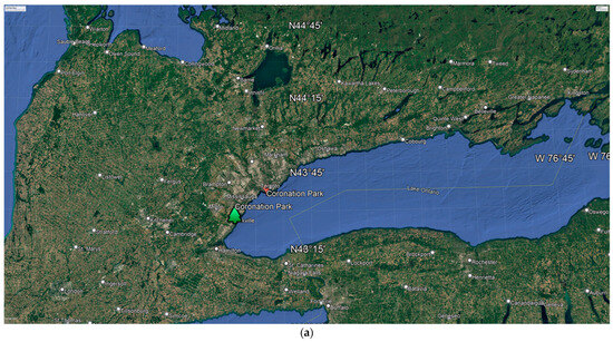
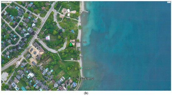
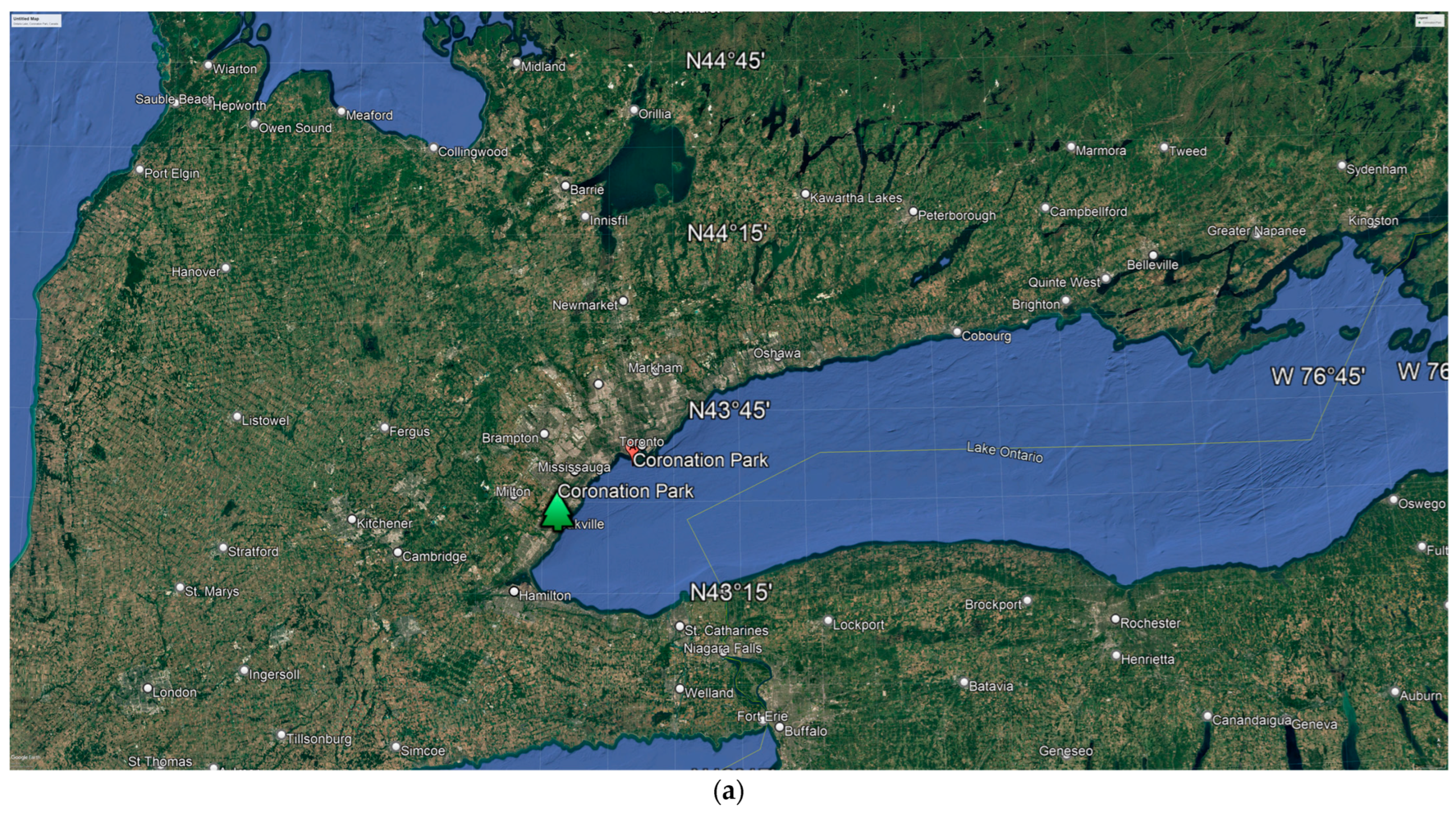
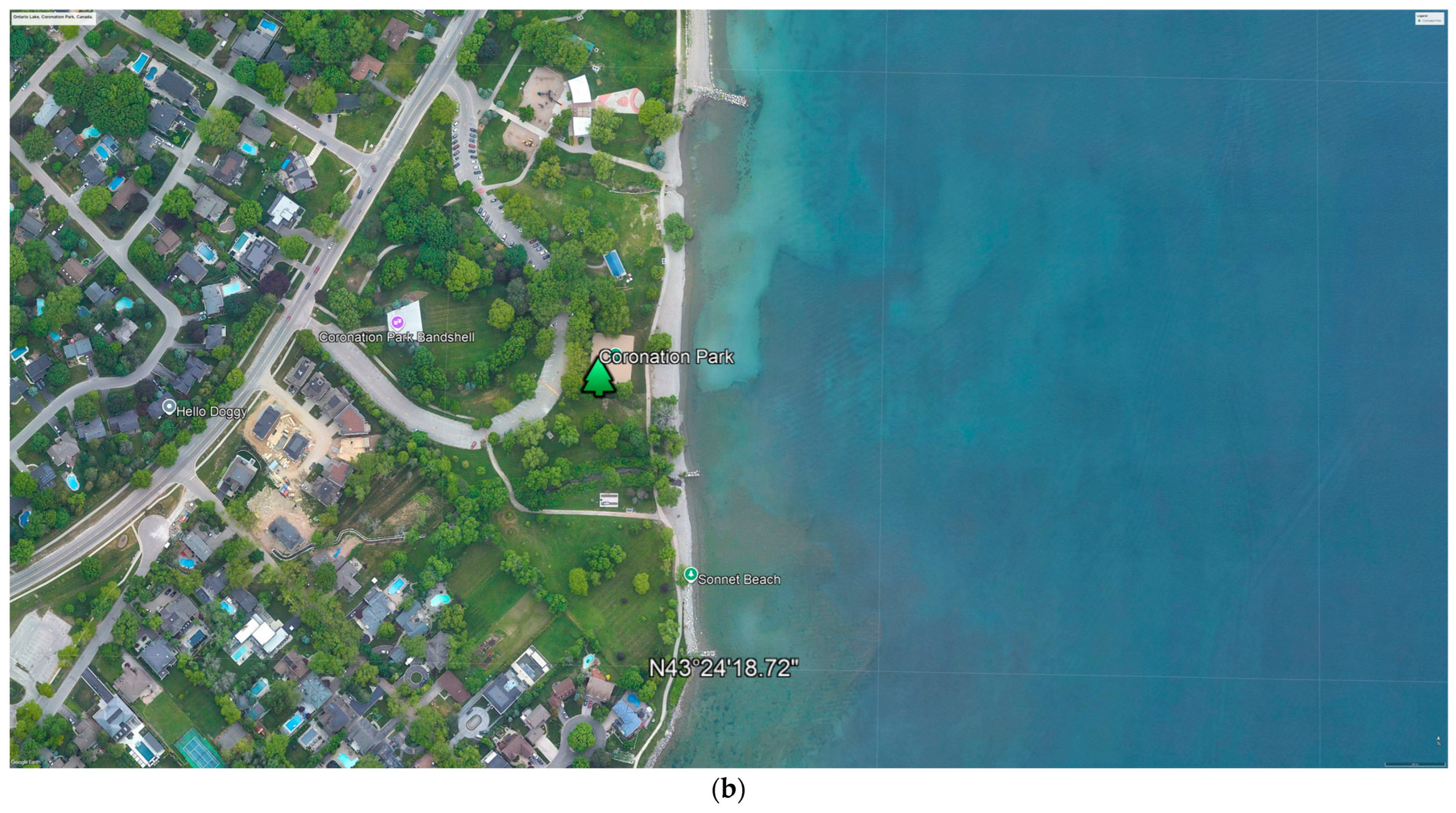
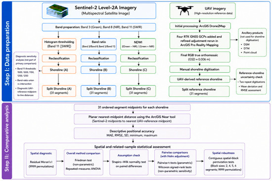
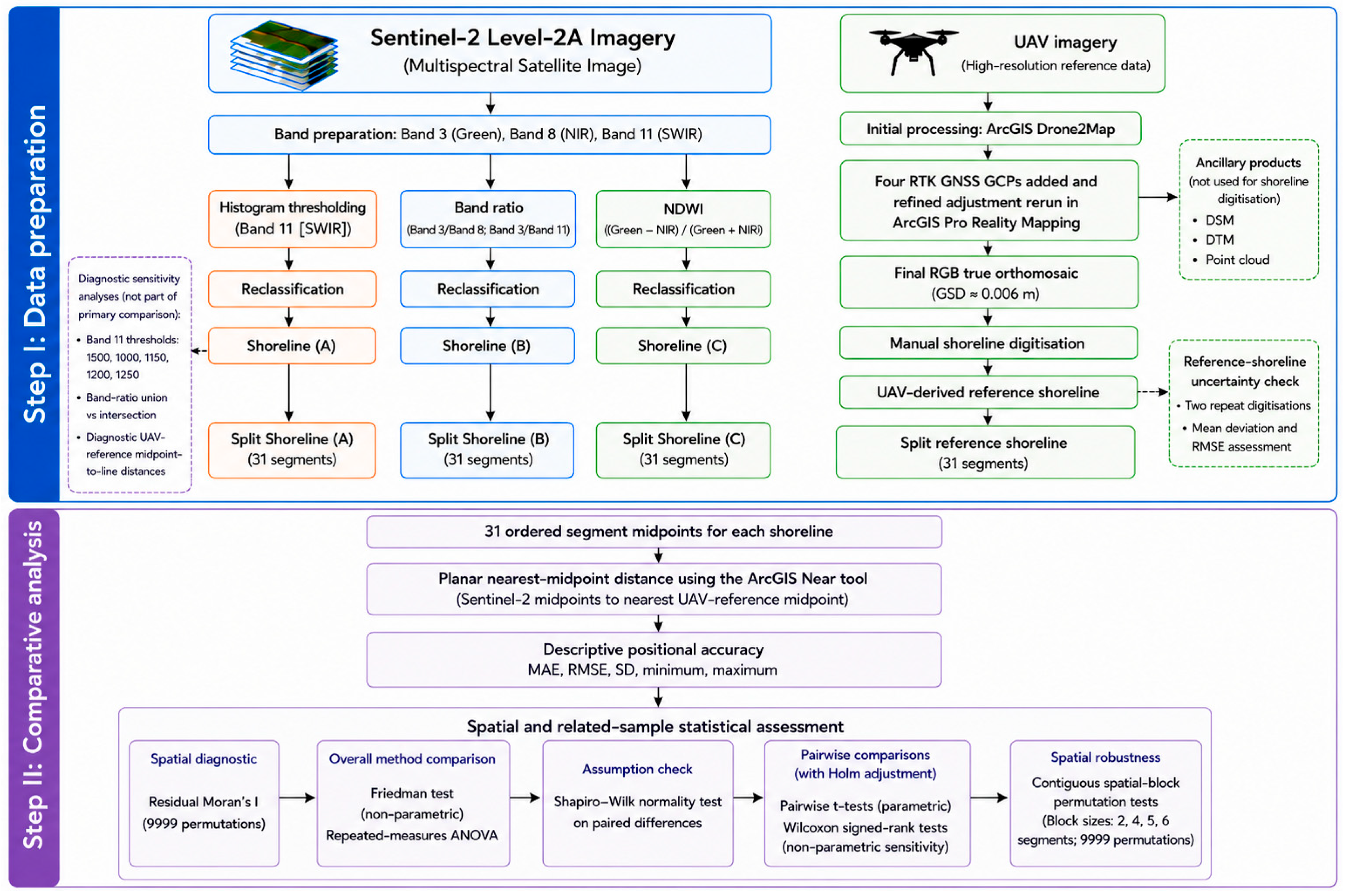
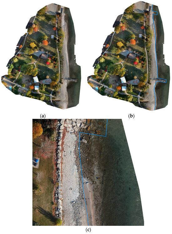
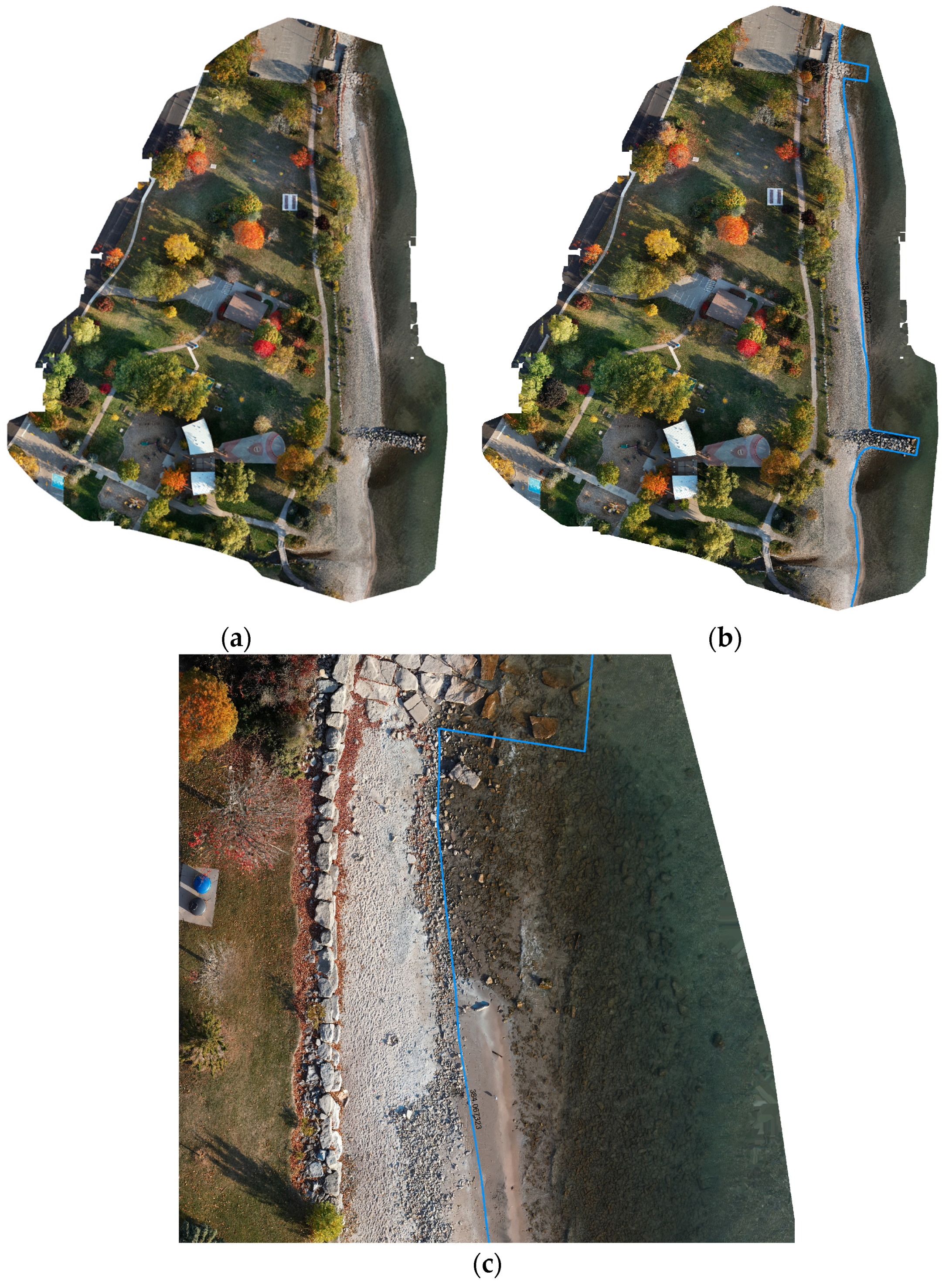
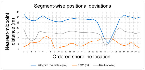
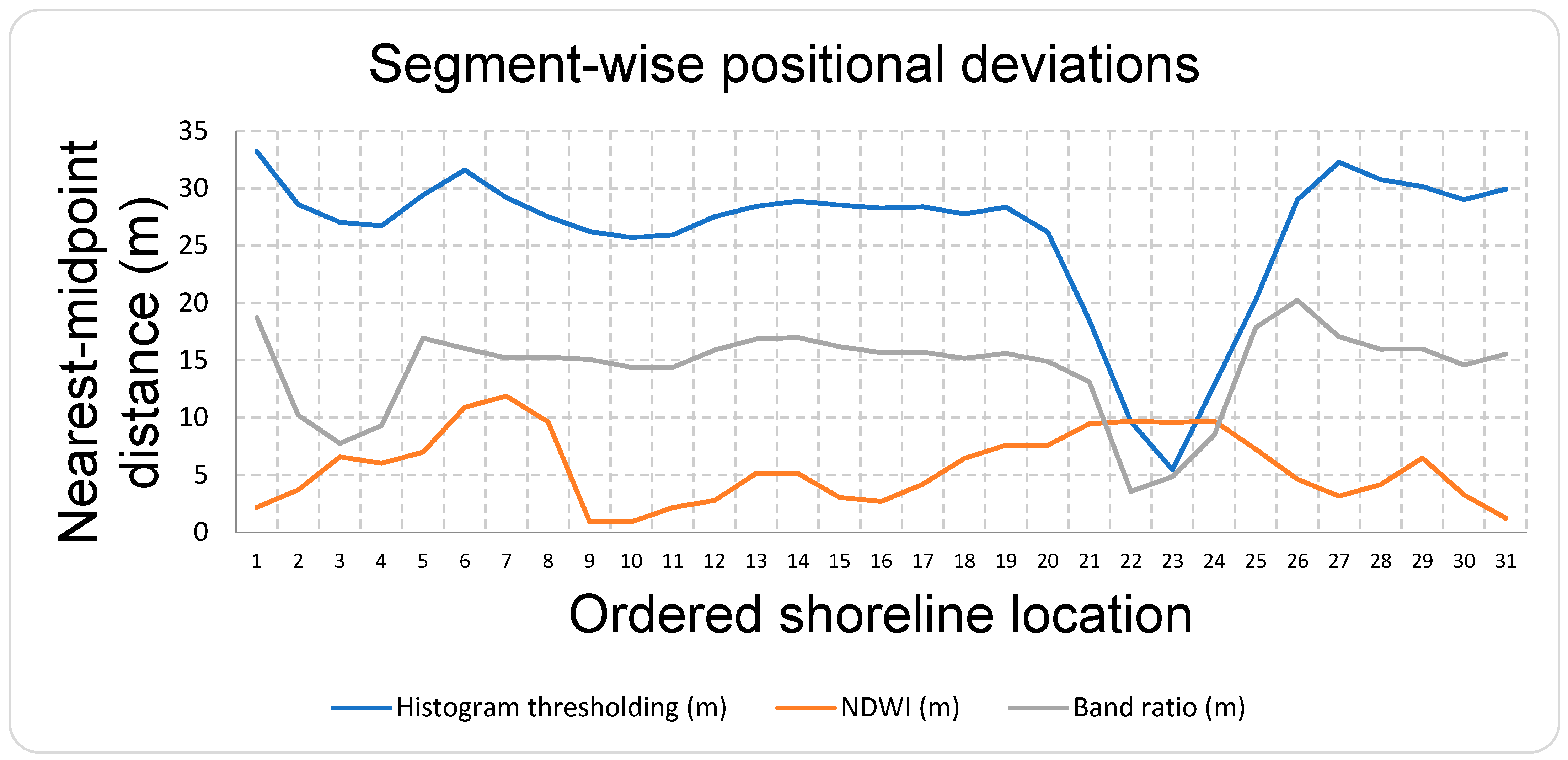
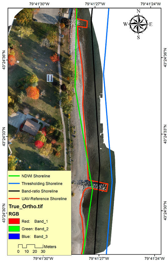
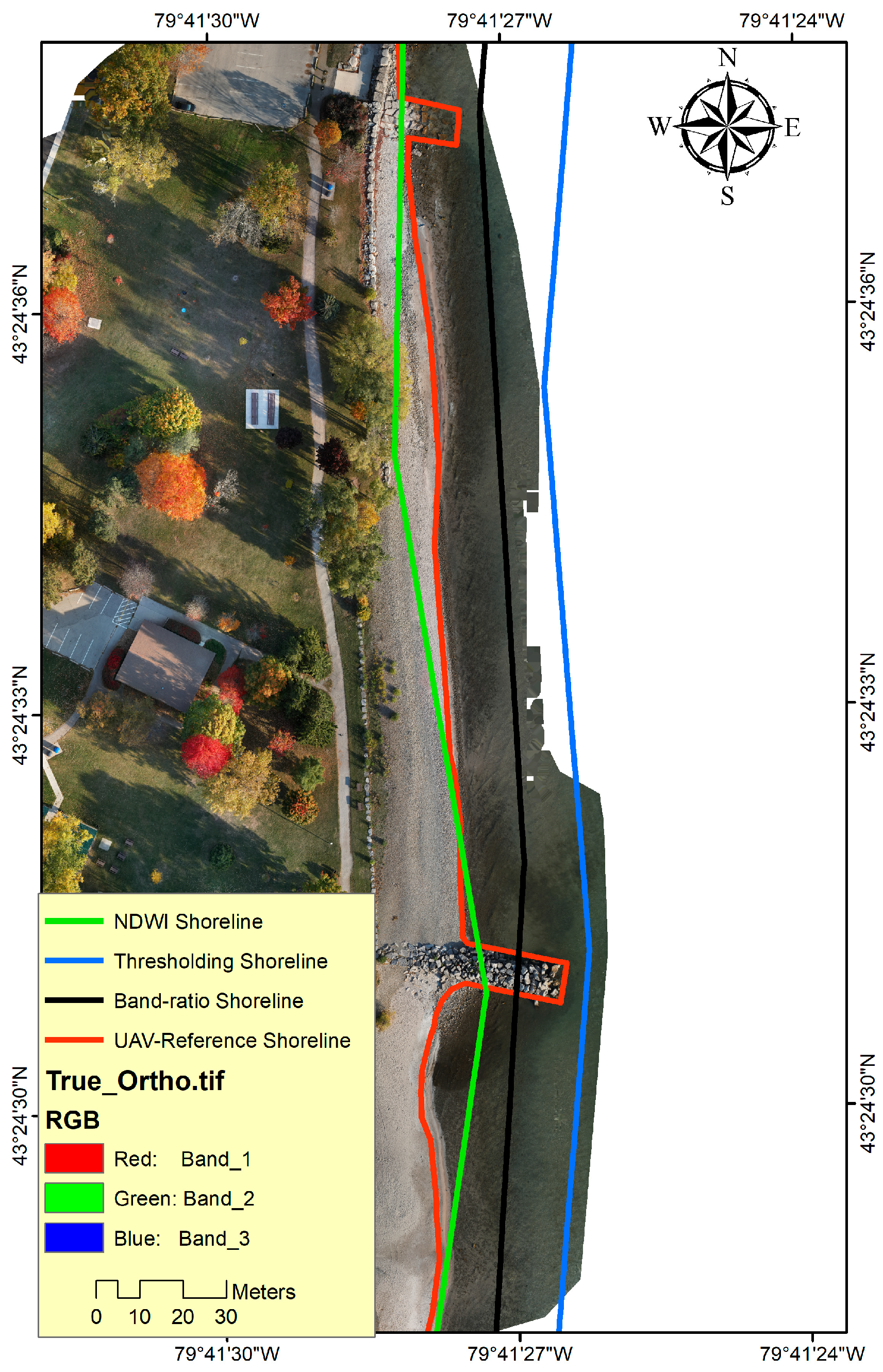

Disclaimer/Publisher’s Note: The statements, opinions and data contained in all publications are solely those of the individual author(s) and contributor(s) and not of MDPI and/or the editor(s). MDPI and/or the editor(s) disclaim responsibility for any injury to people or property resulting from any ideas, methods, instructions or products referred to in the content. |
© 2026 by the authors. Licensee MDPI, Basel, Switzerland. This article is an open access article distributed under the terms and conditions of the Creative Commons Attribution (CC BY) license.