


Abstract
Early diagnosis of colorectal cancer is considered a key factor in reducing the complications of the disease before it spreads throughout the body, which raises survival and increases the chance of patient recovery. This research introduces machine learning and deep learning classifiers trained on a publicly available histopathological dataset with four magnification levels (40×, 100×, 200×, 400×) and uses stratified k-fold cross-validation to classify colorectal cancer into five classes. Features are extracted in two ways: manually and automatically using a Convolutional Neural Network (CNN). Both machine learning and deep learning techniques performed well on the test data. In summary, machine learning using an automatic feature extraction method achieved an accuracy of 89%, Precision of 88%, Recall of 87%, and F1-Score of 87% using a Support Vector Machine (SVM) classifier, while machine learning using a manual feature extraction method achieved an accuracy, Precision, Recall, and F1-Score of 79% using an Extreme Gradient Boosting (XG-Boost) classifier at 200× magnification. On the other hand, the deep learning model ResNet-50 achieved the best result with 97% accuracy, Precision, Recall, and F1-Score using 100× magnification.
1. Introduction
Colorectal cancer (CRC) is the third most prevalent malignancy worldwide and is a leading cause of mortality. It occurs more frequently in men and typically affects individuals aged 45 or older. CRC is characterized by rapid metastasis to various organs, which significantly diminishes overall health and vitality. Unhealthy lifestyle factors, such as alcohol consumption, poor dietary habits, and physical inactivity, are among the primary contributors to the development of colorectal cancer [1,2,3]. The current mortality rate for colorectal cancer is 9.2%. Projections indicate that by 2035, the incidence of colon cancer will increase to 71.5% and that of rectal cancer to 60% [4].
Early diagnosis of colorectal cancer is considered a crucial factor in reducing the complications of the disease and controlling it at an early stage, before it spreads throughout the body. Early detection improves quality of life, reduces the risk of death from the disease, and offers an opportunity for recovery. Researchers worldwide are developing innovative diagnostic methods using Artificial Intelligence (AI) to improve accuracy and reliability. Machine learning and deep learning techniques are widely used for disease prediction and classification [2,5,6,7]. Colorectal cancer is a significant health concern due to its high prevalence and potential threat to human life. Artificial intelligence (AI), including machine learning (ML) and deep learning (DL), has been widely applied to the diagnosis, classification, and prediction of colorectal cancer. AI systems can analyze complex medical data, identify patterns, and assist in decision-making, thereby supporting healthcare professionals in diagnosing diseases at early stages and determining appropriate treatment efficiently and accurately [3]. Machine learning involves training models on large datasets to improve performance over time without explicit programming, while deep learning employs multi-layer neural networks to extract hierarchical features and achieve high-level representations of data. These techniques have proven effective in various medical applications, particularly in supporting accurate and timely diagnosis [8,9,10].
This research develops and evaluates a comprehensive Artificial Intelligence-based framework for multi-class classification of colorectal cancer histopathological images. To date, this is the first systematic comparison of three analytical approaches using the EBHI dataset: traditional machine learning with handcrafted features, a hybrid method combining automatic feature extraction with conventional classifiers, and end-to-end deep learning. The study also examines the influence of various magnification levels (40×, 100×, 200×, and 400×) to identify the optimal setting for capturing diagnostically relevant features, thereby assisting pathologists in selecting the most effective magnification during microscopic examination. In contrast to previous studies that primarily addressed binary classification or limited configurations, this work addresses a five-class classification problem using a large and consistent dataset that offers a more representative analysis of colorectal tissue heterogeneity. This research answers the following questions: (1) How do machine learning, hybrid, and deep learning approaches compare in multi-class colorectal cancer classification? (2) What is the effect of magnification level on classification performance? (3) Which combination of analytical method and magnification level provides the most reliable and clinically valuable results?
The remainder of this paper is structured as follows. Section 2 reviews the literature on the use of Artificial Intelligence techniques and datasets for colorectal cancer diagnosis. Section 3 presents the dataset description, data augmentation, and preprocessing procedures. Section 4 presents the proposed approach. Section 5 discusses and analyses the experimental results. In Section 6, we present the conclusion and outline directions for future work.
2. Literature Review
Many studies aim to speed up and improve the accuracy of colorectal cancer diagnosis as its global prevalence increases. Researchers have focused on artificial intelligence methods for disease diagnosis using machine learning and deep learning techniques. Traditional ML approaches typically depend on handcrafted feature extraction followed by classifiers such as Support Vector Machines (SVM), Random Forest (RF), and gradient boosting methods [11,12]. In contrast, DL techniques, especially Convolutional Neural Networks (CNNs), enable automatic feature learning directly from raw images, capturing complex and hierarchical patterns. Well-established architectures, including VGG-16, ResNet-50, EfficientNet-B1, DenseNet, and InceptionV3 [13,14,15,16,17,18] have demonstrated strong performance in histopathological image classification. While DL methods generally achieve higher accuracy, ML approaches remain valuable for benchmarking and interpretability. This study adopts and systematically compares both ML- and DL-based strategies to provide a comprehensive evaluation for multi-class colorectal cancer classification.
Qi Ke and Wun-She Yap et al. [19] introduced a deep learning framework for classifying colorectal cancer histopathology images using ensemble models based on deep Convolutional Neural Networks (CNNs) and the EBHI dataset. Their methodology included extensive data preprocessing, such as patch cropping, stain normalization, data augmentation, and balancing across various magnification levels. Multiple CNNs were fine-tuned through transfer learning. The best models were selected as base classifiers for the ensemble. The final ensemble, comprising the five top classifiers, achieved high performance across four magnification subsets, with accuracies of 99.11% at 40×, 99.36% at 100×, 99.29% at 200×, and 98.96% at 400×. In addition to accuracy, the model demonstrated strong recall, precision, and F1-score, underscoring its efficacy in classifying histopathological images of colorectal cancer.
Thang Truong Le, Vinh Thuyen Truong, and colleagues [20] examined the use of deep learning for automated multi-classification of colorectal cancer histopathology images derived from hematoxylin and eosin (H&E)-stained slides. The study evaluated several convolutional neural network (CNN) and transformer-based architectures, including ResNet-34, ResNet-50, and Swin Transformer V2, for their performance and efficiency across various colorectal cancer histological classes. ResNet-34 achieved a favorable balance between accuracy and model complexity, reporting an overall accuracy of 85.04%, with top-2 and top-3 accuracies of 96.68% and 99.23%, respectively. ResNet-50 yielded the highest micro-averaged receiver operating characteristic (ROC) area under the curve (AUC) of 0.9933 and an F1-score of 87.51%. The Swin Transformer V2 demonstrated strong class-specific performance, achieving up to 95.83% accuracy in hyperplastic polyp detection and 93.33% accuracy for adenocarcinoma, though it required, albeit greater computational resources. The authors also introduced a two-stage prediction framework, a binary abnormality detector followed by a multiclass classifier, which significantly enhanced classification robustness for underrepresented and morphologically complex classes. For instance, the accuracy for high-grade dysplasia improved from 53.57% to 71.43% using this two-stage approach. These findings underscore the value of moderate-depth deep learning models and hierarchical prediction frameworks for addressing the morphological diversity across colorectal cancer stages and supporting pathology diagnosis.
Qi Ke and Hum Yan Chai et al. [21] proposed an automated deep learning framework for colorectal cancer (CRC) classification, integrating domain-specific transfer learning and multi-model feature fusion. Their model addresses challenges such as multi-scale structures, noisy labels, and class imbalance by extracting relevant features using transfer learning, and then fusing these features through a multi-head self-attention mechanism, followed by an MLP classifier. Evaluated on three datasets, including EBHI, Chaoyang, and COAD, the model achieved high accuracy of 99.68%, 86.72%, and 99.44%, respectively.
Ammar Ahmad Khan et al. [22] proposed a deep learning model to classify colon cancer as benign or malignant using a histopathological dataset. ResNet-101, vision transformer (ViT), Swin Transformer, and the modified Swin Transformer are used to detect colon cancer. They achieved superior performance with the modified Swin Transformer and further improved results by modifying the Swin model’s last layer. The accuracy reached 99.8% on test data for the modified Swin Transformer. It also achieved 99.64%, 99.36%, and 98.27% on the Swin Transformer, ViT, and ResNet-101 models, respectively. The LC25000 dataset was used for training and validation. Anurodh Kumar et al. [23] proposed a new lightweight deep learning method to classify colorectal cancer into 10 classes using the histology dataset and the NCT-CRC-HE-100K dataset. The goal of the proposed deep learning model (CRCCN-Net) was to classify colorectal cancer into multiple classes more quickly and with superior accuracy. They used three datasets for training and testing: the histology dataset with 8 classes, the NCT-CRC-HE-100K dataset with 9 classes, and the merged dataset with 10 classes. The merged dataset consisted of the histology dataset and the NCT-CRC-HE-100K dataset. They used the Xception, InceptionResNetV2, DenseNet121, and VGG16 pre-trained models, as well as the proposed CRCCN-Net model. The proposed model is designed with fewer learning parameters to accelerate training while maintaining performance. The accuracy of the proposed model is 93.50%, 96.26%, and 99.21% on the colorectal histology dataset, the NCT-CRC-HE-100K dataset, and the merged dataset, respectively. The proposed model achieved superior performance compared with existing pre-trained models.
Ahmed S. Sakr et al. [24] introduced a lightweight deep learning approach for classifying colorectal cancer cell images. The authors normalized the input images before evaluation with their proposed model, achieving an accuracy of 99.5%. Aya Hage Chehade et al. [25] implemented machine learning models to classify lung and colon cancer using histopathological images. Their methodology incorporated feature engineering to generate new features from existing data, thereby improving classifier performance, and utilized image preprocessing to facilitate class prediction. The XGBoost classifier attained 99% accuracy and a 98.8% F1-score. The study also evaluated multiple classifiers, including XGBoost, Random Forest (RF), Support Vector Machine (SVM), Linear Discriminant Analysis (LDA), Multilayer Perceptron, and LightGBM. Ying Su et al. [26] developed a machine learning model to estimate survival time in patients with colon cancer. They employed RF, SVM, and Decision Tree (DT) algorithms, along with Lasso-extracted gene features, to determine cancer stages. The RF model demonstrated the highest performance, with an accuracy of 99.81% and an F1 score of 99.68%.
Md. Alamin Talukder et al. [27] proposed a hybrid approach that combines deep and machine learning feature-extraction models to classify colon and lung cancer. Their method achieved impressive accuracy results of 99.05% for lung cancer, 100% for colon cancer, and 99.30% when combining both datasets.VGG16, VGG19, DenseNet169, and DenseNet201 are used to extract features, and RF, SVM, LR, MLP, XGB, and LGB are used to evaluate the performance. Then, the top three classifiers are used in ensemble techniques, such as soft and hard voting, to classify the datasets. The SVM, LR, and MLP were the highest-performing classifiers across all datasets. Mehedi Masud et al. [28] developed a pre-trained convolutional neural network (CNN) model to classify lung and colon cancers using the LC25000 dataset, which comprises five balanced classes per cancer type. Following image processing and feature engineering, the proposed CNN model was trained and validated, achieving a peak accuracy of 96.3%.
Zarrin Tasni et al. [29] implemented a deep learning approach to classify colorectal cancer cell images, training the MobileNetV2 model and variants with max and mean pooling layers. The MobileNetV2 model achieved an accuracy of 99.67%. A. Ben Hamida et al. [30] assessed deep learning models for both prediction and segmentation tasks using histopathological data from 5181 samples. Their results indicated that the ResNet CNN classification model achieved approximately 97% accuracy on the AiCOLO dataset and accuracies of 96.8%, 99.8%, and 99.98% on the CRC-5000, NCT-CRC-HE-100K, and a combined dataset, respectively. Furthermore, U-Net and SEGNET CNN models were evaluated for segmentation tasks on the AiCOLO dataset, with U-Net achieving 76.18% accuracy and SEGNET achieving 81.22% on the training set. When tested on the CRC-5000, NCT-CRC-HE-100K, and WARWICK datasets using the SEGNET model, the accuracies were 98.66%, 99.12%, and 78.39%, respectively.
Zhigang Song et al. [31] introduced a deep learning model to evaluate the alignment between pathologists’ diagnoses and the model’s classification of colorectal cancer histopathological images. They used 177 carefully diagnosed samples to develop their model, utilizing DeepLab v3 and ResNet-34 architectures. The model achieved an area under the curve (AUC) of 92%, demonstrating its ability to accurately diagnose colorectal cancer and yielding results that closely match those of pathologists’ diagnoses. Patrik Sabol et al. [32] developed a Cumulative Fuzzy Class Membership Criterion (CFCMC) classifier to predict the type of colorectal cancer among eight kinds of CRCs using deep learning. Initially, they employed a CNN classifier with a ResNet-50 model, achieving an accuracy of 93.80% without providing interpretability of the model’s output. They then modified the CNN design to map inputs to outputs, enabling an illustrative prediction that highlights image similarities and differences across cancer types. Using an exception architecture, this modified model reached an accuracy of 92.78%. Although the accuracy did not exceed that of existing pre-trained CNN models, the added interpretability feature helps specialists identify cancer types efficiently and accurately. They trained and evaluated their approach on a histopathological dataset collected by Borkowski, A. A et al. [33]. Manabu Takamatsu et al. [34] employed a Random Forest algorithm to predict lymph node metastasis in the first stages of colorectal cancer. Their machine learning approach yielded promising results, achieving 93.8% accuracy on a dataset of 370 whole-slide images of colorectal cancer.
The proposed study introduces a comprehensive AI-based framework for the multiclass classification of colorectal cancer using histopathological images, addressing key limitations identified in the literature. Its novelty lies in the unified integration and systematic comparison of three analytical strategies: (1) traditional machine learning with handcrafted features, (2) a hybrid approach combining CNN-based automatic feature extraction with conventional classifiers, and (3) end-to-end deep learning architectures. Unlike previous studies, which have primarily focused on binary classification (e.g., Hu W. and Li C. [35]) or relied on single strategies or highly complex systems (e.g., Qi Ke and Wun-She Yap et al. [19]), this framework demonstrates competitive performance with a simpler architecture, emphasizing the effectiveness of automatic feature extraction and transfer learning. Additionally, this study tackles a five-class classification task, offering a more comprehensive understanding of colorectal tissue heterogeneity. It also explores the influence of image magnification levels (40×, 100×, 200×, and 400×) on classification performance, an aspect not previously examined in the literature. To ensure robust and unbiased evaluation, the framework employs stratified k-fold cross-validation and data augmentation techniques to address class imbalance. Furthermore, Qi Ke and Hum Yan Chai et al. [21] proposed an automated deep learning framework for CRC classification, integrating domain-specific transfer learning and multi-model feature fusion. Their model effectively addresses challenges such as multi-scale structures, noisy labels, and class imbalance by extracting relevant features via transfer learning and fusing these features through a multi-head self-attention mechanism, followed by an MLP classifier. Evaluated on the three datasets EBHI, Chaoyang, and COAD, it achieved high accuracies of 99.68%, 86.72%, and 99.44%, respectively. This combined approach underscores the potential of advanced deep learning techniques to enhance CRC diagnostic accuracy and robustness.
3. Data Preprocessing
3.1. Dataset
The EBHI (Enteroscope Biopsy Histopathological H&E Image Dataset) for colorectal cancer was provided by two pathologists from the Cancer Hospital of China Medical University and organized by four biomedical researchers. Images were obtained via enteroscope biopsy, stained with H&E, captured using an Olympus microscope (Japan) (eyepiece 10×, objectives 4×–40×), and saved as 2048 × 1536 JPG files using the NewUsbCamera software [35]. The dataset comprises two main categories, Benign and Malignant, with five distinct stages and four magnification levels (40×, 100×, 200×, and 400×), totaling 5203 images. The Benign category includes Normal, polyps, and Low-grade Intraepithelial Neoplasia, while the Malignant category consists of High-grade Intraepithelial Neoplasia and Adenocarcinoma. The dataset is partitioned into training (80%) and testing (20%) sets. Table 1 presents the number of images per class and magnification level. Figure 1 displays a sample from each data class, with all images shown at 40× magnification and a resolution of 2048 × 1536 pixels.
Table 1.
Dataset Description (before augmentation).
Figure 1.
Dataset samples from different colorectal tissue classes (a) Normal. (b) Polyps. (c) Low-grade Intraepithelial Neoplasia. (d) High-grade Intraepithelial Neoplasia. (e) Adenocarcinoma.
In this study, magnification denotes the level at which images are acquired via endoscopic biopsy, specifically using a 10× eyepiece and four objective lens magnifications: 4×, 10×, 20×, and 40×. Correspondingly, the dataset is organized into four magnification categories—40×, 100×, 200×, and 400×—with each level offering a distinct degree of detail. These variations in magnification substantially affect the behavior and performance of the classifiers and analytical models. As illustrated in Figure 2, representative images from each magnification level (40×, 100×, 200×, and 400×) showcase the progressive enhancement of structural detail with increasing magnification. For instance, 40× images provide a general overview of tissue architecture but lack the fine cellular patterns necessary for precise feature extraction, whereas 400× images reveal detailed cellular structures, enriching the dataset but also increasing computational demands due to higher dimensionality. The intermediate magnifications, 100× and 200×, strike a balance by capturing sufficient morphological detail while keeping image size and complexity manageable. Therefore, these magnifications were selected for model training and classification, as they offer an optimal compromise between feature richness and computational efficiency.
Figure 2.
Comparison of four different magnifications.
Table 1 presents the dataset, which is imbalanced in the number of images per class. This imbalance may result in biased learning and an increased risk of overfitting during the modeling stage if not addressed. To resolve this, oversampling techniques were used to improve the representation of minority classes, and stratified k-fold cross-validation (SKCV) was employed for model training and evaluation.
Over-sampling is a technique used to address the significant imbalance in image counts across classes by augmenting the number of instances in underrepresented classes. This is achieved by applying transformations such as rotation, shifting, and flipping the images at different angles. These augmentation strategies artificially increase the dataset size in classes with fewer samples, thereby improving the model’s robustness. For instance, rotating or flipping images by various degrees can effectively enhance the representation of minority classes, thereby reducing classification error rates [6]. However, this method may generate artificial data if the number of additional images is excessive. When the percentage of augmented images becomes too high, it can compromise the dataset’s authenticity, potentially leading to models that perform well on the training data but generalize poorly to unseen data [36].
Stratified k-fold cross-validation is an effective evaluation strategy for datasets with imbalanced class distributions because it preserves the class proportions across all folds. In this approach, the dataset is divided into k folds, with approximately equal proportions of samples from each class in each fold. During each iteration, one fold is used for validation while the remaining () folds are used for training. This procedure is repeated (k) times so that each fold serves once as the validation set. By maintaining consistent class distributions across the folds, the training and validation subsets remain representative of the overall dataset. This helps reduce potential bias toward majority classes and provides a more reliable estimation of model performance. Consequently, stratified k-fold cross-validation improves the robustness and generalizability of the trained models by ensuring that performance evaluation is conducted on balanced, representative data partitions [36]. In this research, data augmentation with 5-fold SKCV was applied. Table 2 shows the number of images after applying the augmentation technique.
Table 2.
Dataset Description (after augmentation).
3.2. Data Preparation
Images must be preprocessed before being inserted into the model to clean them from any noise and transform them into a proper form that can be analyzed to extract their hidden patterns. The preprocessing stage involves several procedures applied to each image, including augmentation, resizing, normalization using a min–max scaler, conversion to grayscale, dataset partitioning, adjustment of color channel margins, filtering, and smoothing. We performed image processing operations to increase the algorithm’s efficiency and enhance the classifier’s performance, in proportion to the dataset’s nature. Figure 3 presents a sample of the data before and after the application of preprocessing operations.
Figure 3.
Data before and after applying some of the pre-processing operations.
3.3. Feature Extraction
Models require features to understand data patterns and predict image classes. Numerous types of features can be derived from images, including the following:
- 1.
- Color Features:
- Color Moments, encompassing statistical measures like mean, variance, and skewness of color channels, provide insights into color distribution. Equations (1)–(3) represent general formulas of means , variance , and skewness , respectively, which are used to extract color features [37].where n is the number of pixels, and is the pixel value.
- 2.
- Texture Features:
- The Grey-Level Co-occurrence Matrix (GLCM) characterizes the spatial relationships among pixel intensities, enabling the extraction of texture features. This matrix quantifies the frequency of specific grey-level variations in an image at defined distances and orientations between pixel pairs [38,39].
- The Grey Level Difference Method (GLDM) measures the intensity values between pixels separated by a specific distance in different directions [40].
- 3.
- Frequency Domain Features:
- The Fourier transform transforms an image into its frequency representation, aiding in capturing periodic patterns. Equation (4) expresses the general formula of the Fourier Transformation [41].where 0 < k < n and = .
- The Wavelet Transform decomposes an image into various frequency components using wavelets.
- 4.
- Convolutional Neural Network (CNN) Features, which are called deep features, can be extracted using the activations of various layers in a trained CNN.
3.4. Performance Metrics
The model’s performance is assessed using a confusion matrix to compare different classifiers and deep learning models. It measures Accuracy, Precision, Recall, F1-score, and Sensitivity. The Equations (5)–(12) for each metric are listed below [42].
where Precision and Recall correspond to the values defined in Equations (6) and (7), respectively.
Since our study considers a multi-class problem with classes, we extend these definitions using per-class metrics and averaging techniques. For each class , we employed a weighted average metric to obtain overall metrics across all classes. Each class is weighted by its number of true samples :
Overall accuracy is calculated as:
4. Methodology
4.1. Environment
All these experiments were implemented using the Python programming language in Google Colab and Kaggle notebooks, leveraging T4 GPUs (Google Colab, Google LLC, Mountain View, CA, USA) in Google Colab and P100 GPUs (Kaggle, Google LLC, Mountain View, CA, USA) in Kaggle. The experiments were performed using Python (v3.10.14) and Python (v3.12.12) on a Dell workstation (Dell Inc., Round Rock, TX, USA) running Windows 10 Enterprise. The workstation features an Intel Core i7-8550U CPU (Intel Corporation, Santa Clara, CA, USA) operating at 1.80 GHz and 8 GB of RAM. Our research aims to use artificial intelligence, specifically the two branches of machine learning and deep learning, to classify a colorectal cancer dataset into five categories across four magnifications. We compare the performance of both machine learning and deep learning techniques in the classification process using the SKCV method. We implemented three main techniques in our method: (1) machine learning with manual features, (2) machine learning with automatic features, and (3) a deep learning technique.
4.2. Machine Learning with Manual Features
The methodology of the proposed machine learning approach is illustrated in Figure 4, and consists of the following steps:
Figure 4.
Structure of the proposed machine learning method with manual/automatic feature extraction.
- 1.
- Data Splitting: The dataset was partitioned into 80% for training and 20% for independent testing. The test set was not used until the final evaluation.
- 2.
- Data Augmentation and Preprocessing: To address class imbalance in the training dataset, an oversampling technique was applied. The original images, sized at 2048 × 1536 pixels, were resized to 512 × 512 pixels to reduce computational load while preserving essential texture details. Subsequently, images were normalized using Min–Max scaling to standardize pixel values and facilitate more reliable model training.
- 3.
- Feature Extraction: A total of 252 handcrafted features were extracted, including:
- Color features
- Texture features (GLCM and GLDM)
- Frequency-domain features (FFT and Wavelet Transform)
All extracted features were included in the modeling phase. The feature selection methods were not applied in this research. - 4.
- Model Training and Evaluation using SKCV: A stratified k-fold cross-validation (SKCV) procedure with 5 folds was implemented exclusively on the training set to maintain class distribution. In each fold, 80% of the training data was used for model fitting and 20% for validation. Ten classifiers, including XGBoost, AdaBoost, Gradient Boosting, K-Nearest Neighbors (KNN), Naïve Bayes, Support Vector Machine (SVM), Multi-Layer Perceptron (MLP), Random Forest, Decision Tree, and Logistic Regression, were trained using SKCV. The final performance metrics were assessed on the independent test set.
- 5.
- Model Selection: The best-performing classifier was selected based on evaluation metrics.
4.3. Machine Learning with Automatic Features
As previously discussed, this approach closely resembles the first method, but employs a different feature extraction technique. The same preprocessing steps used in machine learning with manual features were also applied here. Five pre-trained convolutional neural network (CNN) models were utilized: ResNet-18, DenseNet-121, VGG-16, AlexNet, and EfficientNet-B1. These models were originally trained on the ImageNet dataset, which contains over 1.25 million images. The architecture of CNNs includes convolutional and pooling layers for preprocessing and feature extraction, as well as fully connected layers for image classification. In this study, the fully connected layers were excluded from the model architectures. Features extracted from the convolutional layers were used to train traditional machine learning classifiers [43]. The selection of these models was informed by prior research demonstrating their effectiveness in extracting representative and discriminative features from medical images. During the feature extraction phase, all models were used with their default parameter settings, and no hyperparameter tuning was performed.
After preparing the dataset by resizing and splitting it into 80% for training and 20% for testing sets, we extracted automatic features for each set. Then, we applied Stratified K-Fold Cross-Validation on the training set and input the features into the classifiers. The classifiers’ performance was evaluated on the test set, as illustrated in Figure 4. The number of features extracted from the employed pre-trained models is presented in Table 3. This method achieved satisfactory performance evaluation with our dataset.
Table 3.
Number of features extracted from the pre-trained models.
4.4. Deep Learning Models
In this method, we employed five well-known pre-trained deep learning architectures (ResNet-50, DenseNet-121, VGG-16, InceptionV3, and EfficientNet-B1) to classify the dataset. The overall workflow of the proposed deep learning approach is illustrated in Figure 5, and consists of the following steps:
Figure 5.
Structure of the proposed Deep Learning classification model.
- 1.
- Data Splitting: The dataset was partitioned into 80% for training and 20% for independent testing. The test set was not used at any stage of model training or optimization.
- 2.
- Data augmentation and Preparation: An oversampling technique was applied to the training dataset. The images were resized to match the input size requirements of the selected CNN architectures and organized before training.
- 3.
- Training Models with applying Stratified K-Fold Cross-Validation (SKCV): A 5-fold stratified K-fold cross-validation was applied exclusively to the training set to preserve the class distribution across folds. In each fold, the model was fine-tuned using transfer learning. Hyperparameter tuning (e.g., learning rate, batch size, number of epochs, and optimizer settings) was performed using a grid search.
- 4.
- Model Selection: The optimal configuration was determined by averaging validation performance across all five folds.
- 5.
- Final Evaluation: The selected model was evaluated using the independent test set to determine its generalization performance.
- 6.
- Model Saving: The final optimized model was preserved to facilitate future deployment.
Hyperparameter Tuning: Deep learning models, such as Convolutional Neural Networks and Artificial Neural Networks, typically employ similar network architectures and standard hyperparameter sets, which substantially affect their performance. Adjusting hyperparameter values is fundamental to enhancing model outcomes in deep learning. Among these, the learning rate is particularly important, as it determines the magnitude of parameter updates at each iteration and facilitates convergence of the cost or loss function to its minimum. The loss or cost function measures the discrepancy between predicted and actual output values. A high learning rate can accelerate training but may cause the model to overshoot the minimum error. In contrast, a low learning rate may lead to convergence to a suboptimal solution and increase training time. Selecting an appropriate learning rate is therefore essential to minimize error within a reasonable timeframe [44].
Batch size is a crucial hyperparameter in deep learning models, as it determines the number of data samples processed per parameter update. Other integral hyperparameters include the number of hidden layers, dropout rate, activation function, and optimization technique. The number of hidden layers reflects the complexity of the dataset and influences the model’s capacity to learn from the data. Standard activation functions, such as ReLU, are selected based on factors including the dataset type (binary or multi-class) and the neural network architecture. Activation functions enable the model to transition from linear to nonlinear behavior, thereby allowing it to extract more complex features from data. The choice of optimizer is also critical to model performance. Among available optimizers, the Adaptive Moment Estimation (Adam) optimizer is widely used due to its demonstrated effectiveness [44]. Hyperparameter tuning techniques include grid search, manual adjustment based on experimental results, and reference to prior studies. In this study, the grid search technique was employed to optimize performance.
5. Experimental Results and Discussion
This section introduces the experimental results of our methodology for three scenarios in detail. It is split into three subsections: (1) Results and discussion of machine learning with manual feature extraction, (2) results and discussion of machine learning with automatic feature extraction, and (3) deep learning results.
5.1. Experimental Results of Machine Learning with Manual Features
Following oversampling and preprocessing, which included normalization, standardization, and color conversion as required, color features and texture features were extracted. Specifically, the grey-level co-occurrence matrix (GLCM) was computed with a distance of 1 and angles of 0°, 45°, 90°, and 135°. The grey-level difference method (GLDM) was calculated with a distance of 10 pixels in four directions: horizontal, vertical, diagonal (top-right), and diagonal (bottom-left). Frequency-domain features, including wavelet and Fourier transforms, were also extracted, yielding a total of 252 features. Stratified k-fold cross-validation with five folds was then applied. Subsequently, classification was performed using ten established machine learning classifiers. The oversampling technique utilized the following parameters: rotation range of 0.5, shear range of 0.1, zoom range of 0.1, and horizontal flip.
Table 4 summarizes the weighted average performance of the experiments for each magnification on the validation set across five folds and on the testing set. Manual feature-based models evaluated at different magnification levels (40×, 100×, 200×, and 400×) exhibited varying classification performance. At 40× magnification, the Logistic Regression (LR) classifier achieved a validation accuracy of 75.17 ± 1.53% and a test accuracy of 67%, with precision, recall, and F1-score of 69%, 67%, and 68%, respectively. At 100× magnification, the LR model demonstrated a validation accuracy of 88.64 ± 1.81% and a test accuracy of 70%, with precision, recall, and F1-score values of 70%, 70%, and 69%, respectively. The highest performance was obtained at 200× magnification with the XGBoost classifier, which achieved a test accuracy of 79%, and precision, recall, and F1-score values all at 79%, indicating balanced classification. At 400× magnification, the LR classifier achieved a test accuracy of 77%, with precision, recall, and F1-score values of 76%, 77%, and 77%, respectively. Overall, the 200× magnification level combined with the XGBoost classifier provided the most stable and highest test performance among the evaluated configurations.
Table 4.
Performance evaluation for manual Features, all magnification levels for validation and testing sets.
The performance of the evaluated machine learning classifiers differs across the four magnification levels (40×, 100×, 200×, and 400×), as shown in Figure 6. At 40× magnification, classification accuracy is moderate, with Logistic Regression (LR) achieving the highest accuracy at 67%, followed by Support Vector Machine (SVM) at 65.48% and Gradient Boosting at 64%. Naïve Bayes demonstrates the lowest performance at 12%. At 100× magnification, accuracy improves slightly, with LR again achieving the highest accuracy at 70%, followed by XGBoost at 64% and Gradient Boosting at 59%. At 200× magnification, a marked improvement is observed, with XGBoost achieving the highest accuracy at 79%, followed by LR (78%), SVM (77%), and Gradient Boosting (77%). This suggests that 200× magnification provides more discriminative information for classification. At 400× magnification, performance decreases slightly compared to 200×, with LR maintaining the highest accuracy (77%), followed by XGBoost (70%) and Gradient Boosting (68%).
Figure 6.
Performance of ML models with manual features across all magnification levels.
These results indicate that 200× magnification offers the most informative representation of tissue structures, allowing machine learning classifiers to extract more discriminative features. Lower magnification levels, such as 40×, may omit critical cellular details, whereas very high magnification (400×) may emphasize local structures and reduce contextual information. Logistic Regression consistently demonstrates strong, stable performance across most magnification levels, likely because it effectively separates classes when the extracted manual features are sufficiently discriminative and linearly separable. Ensemble methods, including XGBoost and Gradient Boosting, also perform well at higher magnifications, likely because they capture complex feature relationships and enhance classification robustness. We used default hyperparameter settings for all machine learning classifiers to allow a fair comparison within the SKCV framework. Unless noted otherwise, we kept the configurations as provided by the Scikit-learn library. For the Random Forest classifier, we used the default parameters and set the random state to 42 for reproducibility. Logistic Regression was trained for 1000 iterations. The Multi-Layer Perceptron (MLP) had one hidden layer with 100 neurons, ReLU activation, the lbfgs solver, alpha set to 0.0001, automatic batch size, a constant learning rate of 0.001, a maximum of 200 iterations, momentum of 0.9, early stopping turned off, and the random state set to 42. By keeping these settings consistent, we ensured that our comparison focused on each classifier’s learning abilities under the same experimental conditions.
Confusion Matrix and Precision–Recall Curves for 200× Magnification
Figure 7 shows the confusion matrix for the XG-Boost classifier tested at 200× magnification. The model distinguishes five histopathological categories: Normal (0), Polyp (1), Low-grade Intraepithelial Neoplasia (2), High-grade Intraepithelial Neoplasia (3), and Adenocarcinoma (4). The classifier performed well at detecting Adenocarcinoma (131 samples) and Low-grade IN (98 samples), both of which are clinically important. It correctly identified 37 Polyp cases, but some were misclassified as Normal (1) or Low-grade IN (7), which suggests these categories share similar features. For the Normal class, 4 samples were correctly predicted, and 4 were misclassified as Polyps. In the High-grade IN class, 8 out of 26 samples were correctly classified. These misclassifications show that adjacent pathological stages can look similar, making accurate classification difficult.
Figure 7.
Confusion Matrix for XG-Boost classifier using manual features on the test data at 200× magnification.
Figure 8 presents the Precision–Recall (PR) curves for the test dataset, illustrating the XGBoost model’s performance across five histopathological classes. The model demonstrates strong performance for Class 2 (Low-grade IN, Average Precision (AP) = 86%) and Class 4 (Adenocarcinoma, AP = 92%), maintaining high precision as recall increases. In contrast, Class 0 (Normal, AP = 42%) and Class 3 (High-grade IN, AP = 39%) exhibit a decline in precision with increasing recall, indicating greater difficulty in distinguishing between classes with similar features. Class 1 (Polyp, AP = 83%) achieves moderate results, balancing precision and recall. Overall, the PR curves indicate that the model effectively detects advanced pathological classes but encounters challenges with early-stage or morphologically similar categories. These findings highlight the need for improved feature representation to enhance the classification of the more challenging classes.
Figure 8.
Precision–Recall (PR) curves for the multi-class classification using the XG-Boost Classifier.
5.2. Experimental Results of Machine Learning with Automatic Features
To improve the performance of machine learning algorithms, automatic features, also referred to as deep features, were extracted using convolutional neural networks (CNNs). The data were prepared and preprocessed before being input into various CNN architectures, including ResNet-18, DenseNet-121, VGG-16, AlexNet, and EfficientNet-B1. The number of features extracted differed across models. Stratified K-Fold Cross-Validation was applied to the training data, and classifier performance was evaluated using the test data.
The experimental results in Table 5 demonstrate a clear impact of magnification level on classification performance. All reported metrics are expressed as weighted averages. At low magnification (40×), the model achieved high validation accuracy but relatively lower test performance. Precision, recall, and F1-score were 75%, 74%, and 74%, respectively. This indicates that global tissue structures alone are insufficient for robust generalization. As magnification increased to 100× and 200×, performance improved significantly. At 200×, test accuracy reached 89.42%. Precision, recall, and F1-score were high at 88%, 87%, and 87%, respectively. These results suggest that intermediate magnification provides a balanced representation of both structural and cellular features. Similarly, 100× produced comparable results, with precision, recall, and F1 scores of 90%, 89%, and 88%, respectively. At the highest magnification (400×), the model achieved the best F1-score (89%), with precision and recall of 89% and 88%. This reflects improved class-wise discrimination due to detailed cellular information; however, a slight decrease in overall accuracy was observed. This trend indicates that classification performance improves from low to intermediate magnifications and stabilizes at higher magnifications. The trade-off shifts toward global context and fine-grained cellular details. Such behavior is consistent with findings in computational pathology, where magnification is a key factor influencing feature representation and model performance.
Table 5.
Performance evaluation for automatic Features, all magnification levels for validation and testing sets.
Figure 9 demonstrates that both classifier type and magnification level significantly affect classification performance. At low magnification (40×), all classifiers achieve low accuracy and high variability, reflecting limited feature representation. As magnification increases to 100× and 200×, accuracy consistently improves for all classifiers, with 200× yielding the highest overall performance. Specifically, SVM achieves the highest accuracy at 89.42%, and most classifiers surpass 85%, indicating that intermediate magnification optimally balances global tissue architecture and cellular-level detail. At 400× magnification, performance remains high but does not improve further, with minor fluctuations in some classifiers, likely due to reduced contextual information. SVM consistently demonstrates the most stable and superior performance across all magnification levels, likely due to its ability to construct optimal decision boundaries, handle high-dimensional feature spaces, and capture non-linear relationships via kernel functions. In contrast, classifiers such as AdaBoost and Naïve Bayes consistently underperform, suggesting limited robustness to varying feature representations.
Figure 9.
Performance of ML models with automatic features across all magnification levels (using ResNet-50).
The improvements seen in our results support the use of Convolutional Neural Networks (CNNs) for feature extraction, which helps to make the representations more distinctive. Combining CNN-based feature extraction with Support Vector Machine (SVM) classification also allows for more accurate modeling of the data and improves classification reliability.
Confusion Matrix and Precision–Recall Curves
The confusion matrix for the SVM classifier at 200× magnification, shown in Figure 10, shows how well each class is identified by comparing actual and predicted labels. Most samples are classified correctly, as indicated by the strong diagonal in the matrix. Classes 4 and 2 have the highest number of correct predictions, suggesting that features at this magnification help separate these classes. Some misclassifications occur, mainly between neighboring classes such as class 0 and class 1, and class 2 and class 3. This means the model sometimes confuses classes with similar histopathological features, especially those close in disease progression. Class 0 has fewer correct predictions, suggesting that normal tissue may appear similar to early abnormal classes. Overall, the confusion matrix shows that the SVM model performs well and that its errors match the data. It is a helpful tool for confirming correct predictions and seeing where mistakes happen across the classes.
Figure 10.
Confusion Matrix for SVM classifier using automatic features on the test data.
The precision–recall curves for the SVM classifier in Figure 11 show strong and consistent performance across several classes, demonstrating its ability to distinguish important histopathological categories. Class 4 (adenocarcinoma) stands out, with its curve remaining at the top of the plot, indicating that the model maintains very high precision even when recall is high. Class 2 (Low-grade IN) also performs well, with its curve showing high precision across many recall values, suggesting clear separation and reliable predictions. Class 1 (polyps) shows good results too, with a balanced curve and only small drops in precision at higher recall, indicating steady detection with few false positives. These findings suggest that the SVM model works especially well for classes that are clearly defined and easy to separate. While there is some variation in other classes, the overall curves show that the model captures important features and achieves high precision at most recall levels. This supports the SVM classifier’s ability to make reliable and accurate predictions in multiclass colorectal cancer histopathological classification.
Figure 11.
Precision–Recall (PR) curves for a multi-class classification model using the SVM Classifier for testing data.
5.3. Experimental Results of Deep Learning
Deep learning is a key concept in our study, along with machine learning. Initially, the images were resized and divided into training (80%) and testing (20%) sets. During training, we applied 5-fold stratified cross-validation on the training set to tune hyperparameters and optimize model performance. This approach ensures that the model learns effectively while maintaining a separate test set for unbiased evaluation. In conjunction with the Adam optimizer, we used different CNN architectures, including ResNet-50, DenseNet-121, VGG-16, InceptionV3, and EfficientNet-B1. We adjusted the batch size, learning rate, optimizer, number of hidden layers, activation function, dropout rate, and epochs multiple times to obtain satisfactory results, treating each magnification level separately. We experimented with various hyperparameter values for each model at different magnifications, running numerous trials to improve performance from approximately 91% to around 97% for the 100× magnification set. Table 6 shows the parameter values that achieved the best performance, and Table 7 presents the performance of the CNN models across all magnifications on the test data.
Table 6.
Hyperparameter values that yield the best performance.
Table 7.
Performance evaluation of CNN models at different magnification levels (%) for validation and test sets.
The deep learning approach achieved the highest overall performance compared to traditional machine learning methods, regardless of whether manual or automatic feature extraction was used. Although deep learning models require greater computational resources, they exhibit superior capacity to capture complex patterns and discriminative features in histopathological images, thereby improving classification accuracy. In contrast, traditional machine learning methods rely primarily on manually engineered features, which can limit their ability to capture intricate image characteristics. Consequently, deep learning represents the most effective approach for this dataset, offering more accurate and reliable classification outcomes.
Table 7 and Figure 12 present the model performance on the dataset. ResNet-50 demonstrated the highest accuracy at 100× magnification. Model performance varied across magnification levels (40×, 100×, 200×, and 400×). At 40×, all models exhibited the lowest accuracy, ranging from 73% to 82%, suggesting that this level of detail is insufficient for reliable feature distinction. At 100×, accuracy increased substantially for all models, surpassing 94%. This magnification appears to offer an optimal balance between tissue structure and cellular detail, thereby facilitating robust feature learning.
Figure 12.
Deep Learning models’ performance for all magnification levels.
At 200× magnification, model accuracy declined slightly compared to 100×, with values ranging from 84% to 91%. This outcome suggests that while cellular detail increases, the loss of broader tissue context may limit the models’ ability to generalize. At 400×, accuracy decreased further, and results became less consistent across models, indicating that excessive magnification introduces highly specific information without enhancing classification accuracy. DenseNet121 and ResNet-50 consistently demonstrate superior performance across all magnifications, reflecting effective feature reuse and robustness. In contrast, VGG16 exhibits lower performance, especially at lower magnifications, which suggests a limited capacity to capture complex hierarchical features. Furthermore, all models display a consistent trend: performance increases from 40× to 100× magnification, then gradually declines at higher magnifications. These results confirm that magnification significantly influences model effectiveness.
These findings are consistent with previous studies, which show that analyzing histopathological images requires balancing global structure at lower magnifications with detailed cellular features at higher magnifications. The results show that 100× magnification is best for deep learning models, as it offers the most useful view of tissue morphology while keeping the model stable and classification accuracy high. This directly supports the goal of finding the best magnification level for the EBHI dataset.
5.3.1. Confusion Matrix and Precision–Recall Curves at 100×
The confusion matrix for the ResNet50 model at 100× magnification in Figure 13 shows strong and reliable classification across most histopathological classes. For Class 0 (Normal), the model correctly classifies 88 samples and misclassifies only 1 as Class 1 (Polyp), showing high precision and recall. Class 2 (Low-grade IN) is perfectly classified, with all 63 samples correctly identified. Class 3 (High-grade IN) also performs well, with 30 correct classifications and just 1 misclassified as Class 2, suggesting little overlap between these two classes. For Class 1, the model correctly identifies 13 samples, while 3 are misclassified as Class 2, indicating some similarity between the classes but still good overall performance. Class 4 (Adenocarcinoma), though it has fewer samples, is also well classified, with 5 correct predictions and only 1 misclassified as Class 3, demonstrating strong detection despite class imbalance.
Figure 13.
Confusion Matrix for ResNet-50 model on test data.
Overall, most values in the confusion matrix are along the diagonal, showing that the model makes correct predictions in most cases. Most misclassifications happen between neighbouring classes, such as Class 1 and Class 2 or Class 3 and Class 2. This is likely because these classes have similar features, especially in the progressive stages of colorectal cancer, which are harder to tell apart. These results show that 100× magnification provides a clear view of the model, helping ResNet50 capture both the overall tissue structure and important cellular details for accurate classification. The model is especially good at distinguishing well-represented, clearly distinct classes.
The precision–recall curves in Figure 14 indicate strong, consistent classification performance across most histopathological classes, underscoring the effectiveness of the proposed model. The Adenocarcinoma and Normal classes maintain precision values near 1.0 at high recall levels (83% and 99%, respectively), which demonstrates highly reliable detection with minimal false positives. The Low-grade intraepithelial neoplasia class achieves perfect recall (100%) and high precision (94%), reflecting the model’s capacity to correctly identify all relevant samples in this category. The High-grade intraepithelial neoplasia class also exhibits robust performance, with balanced precision and recall values (97%), indicating stable and accurate classification with minimal trade-off between sensitivity and specificity. In contrast, the Polyp class shows slightly lower performance, with a recall of 81% and a precision of 0.93, suggesting that although predictions remain accurate, some true instances are not fully detected.
Figure 14.
Precision–Recall curve for a multi-class classification model using ResNet-50 on test data.
Overall, the PR curves confirm that the model achieves high precision across a wide range of recall values for most classes. This behavior indicates strong discriminative capability and reliable classification performance, particularly for clinically significant classes such as Adenocarcinoma. These results further validate the model’s effectiveness in multi-class classification of colorectal cancer histopathological images.
5.3.2. Discussion
This study examined the impact of magnification levels on colorectal cancer histopathological image classification using three approaches: machine learning (ML) with manual feature extraction, ML with automatic feature extraction, and deep learning (DL) with pre-trained models. The primary objective was to determine the optimal magnification level for clinical application in hospital automatic diagnosis systems, balancing accuracy and computational efficiency.
Machine learning (ML) utilizing manual feature extraction achieved a weighted accuracy of 79% at 200× magnification. This outcome suggests that increased magnification enhances cellular detail, although handcrafted features may limit the model’s ability to capture broader contextual patterns. In comparison, ML with automatic feature extraction achieved higher weighted accuracies of 89.26% at 100× and 89.42% at 200×. Although the improvement is modest, these results indicate that 200× magnification offers slightly more discriminative information, allowing the model to leverage both local cellular detail and global tissue context.
Deep learning models outperformed both machine learning (ML) approaches, with ResNet achieving a weighted accuracy of 97.07% at 100× magnification. This finding is consistent with the results of Hu Weiming, Li Chen et al. [35], who reported that deep learning methods outperform traditional ML methods on the same dataset. Our study builds upon this prior work by systematically evaluating multiple magnifications and learning paradigms. Notably, ML with automatic feature extraction strikes a strong balance between accuracy and computational efficiency, making it particularly suitable for real-time clinical deployment in settings with limited computational resources.
These results are consistent with earlier studies on magnification effects. Qi Ke and Wun-She Yap et al. [19] found that ensemble deep learning accuracy was slightly higher at 100× than at 200× on the EBHI dataset (99.36% compared to 99.29%). This supports the idea that intermediate to higher magnification levels offer the best discriminative information. However, their ensemble method requires more computational resources and is more complex, whereas our deep learning approach achieves similar accuracy with a single model. Thang Truong Le and Vinh-Thuyen Nguyen-Truong et al. [20] also demonstrated the benefits of capturing both structural and cellular features, though their work focused more on model design than on selecting the optimal magnification. In contrast, our study directly identifies the magnification level that yields the best results for each learning method, using a simpler approach. The results show that using 200× magnification slightly improves machine learning performance with automatic features, while 100× magnification works best for deep learning methods. This balance between cellular detail and tissue context helps support accurate and efficient automatic diagnosis in clinical settings.
Additionally, a recent study by Qi Ke and Hum Yan Chai et al. [21] introduced a histopathological classification framework for colorectal cancer that employs domain-specific transfer learning in conjunction with multimodal feature fusion to improve diagnostic accuracy. This approach utilizes transfer learning methods specifically tailored to the histopathology domain, enabling the effective extraction of features from histopathological images. The multimodal fusion component integrates diverse feature sources, thereby enhancing classification robustness across multiple datasets. The method demonstrated high accuracy, underscoring the value of combining advanced deep learning techniques with domain-specific modifications for precise colorectal cancer diagnosis. Based on these insights, the current research highlights the importance of multi-magnification analysis and systematically compares manual and automated feature extraction methods. This study evaluates the performance of machine learning classifiers, including support vector machines (SVM) and XGBoost, as well as deep learning models such as ResNet-50, across various magnification levels, with particular attention to 100× magnification. The findings highlight the importance of image resolution and feature representation in early colorectal cancer detection. The focus on multi-scale analysis, comprehensive feature extraction strategies, and comparative evaluation of machine learning and deep learning approaches offers valuable insights for optimizing histopathological classification to achieve improved clinical outcomes.
Figure 15 shows Grad-CAM visualizations, highlighting the main regions that the convolutional neural network focuses on when classifying colorectal histopathological images into five categories at four magnification levels: 40×, 100×, 200×, and 400×. At 40×, the heatmaps cover larger areas and mainly show the overall tissue structure. For Class 1 (Normal), the model highlights regions with even glandular patterns and minimal cell division, matching the typical single-layer epithelial structure. As the magnification increases to 100× and 200×, the highlighted areas become more focused. In Class 2 (Polyp), the model points to raised mucosal areas with a clear lumen and slightly larger nuclei, which fit the polypoid shape. For Class 3 and Class 4 (Low- and High-grade IN), the heatmaps highlight areas with irregular gland shapes and tightly packed nuclei, indicating nuclear displacement and abnormal cell division typical of intraepithelial neoplasia. For Class 4 (High-grade IN), the model mainly focuses on the upper epithelial layers, where changes in nuclear shape and layering are most obvious. At the highest magnification (400×), fine-grained cellular features are captured. The model specifically targets the nuclear-cytoplasmic ratio and luminal distortion in Class 5 (Adenocarcinoma), particularly in areas showing infiltrative growth and glandular disarray, consistent with the aggressive histopathological traits of malignancy. The highlighted regions across all classes confirm that the model focuses on clinically relevant histological cues, including nuclear morphology, glandular patterns, and structural abnormalities. This supports the interpretability of the CNN model, demonstrating its ability to learn and distinguish pathologically significant features across various magnifications for accurate colorectal cancer classification.
Figure 15.
Grad-CAM visualizations.
5.3.3. Limitations and Threats of AI in Medical Diagnostics
AI has the potential to improve diagnostic accuracy and efficiency, but several important challenges remain regarding its clinical use. One major issue is the quality and diversity of training data. When AI models are trained on similar datasets, they often do not work well for different populations, imaging methods, or demographic groups. This can cause performance gaps and diagnostic errors, especially for underrepresented groups. Another problem is that many deep learning systems are difficult to interpret, so clinicians may not understand how AI makes decisions. This lack of transparency can reduce trust and slow down adoption in clinics. There are also ongoing ethical and regulatory concerns, such as protecting patient privacy, complying with evolving medical device regulations, and ensuring accountability when AI influences patient care. Automation bias is another risk: clinicians might rely too much on AI, miss errors, or fail to use their own judgment, which could harm patients. Many AI diagnostic tools also lack thorough external validation, clinical trials, and ongoing monitoring, which means their performance could get worse over time or in new settings. To address these issues, we need several strategies, including building more understandable models, using strong validation methods in different environments, improving data management, and setting clear rules and ethical standards so that AI helps rather than harms patient care [45,46,47].
In this study, the use of a single-source dataset (EBHI) may limit the generalizability of the results across different clinical environments, where variations in staining protocols, imaging devices, and patient populations exist. Although stratified k-fold cross-validation was applied to improve robustness, further validation on multi-institutional datasets is required.
6. Conclusions
This study proposed an AI-based framework for multi-class differentiation of colorectal cancer histopathological images using machine learning, hybrid, and deep learning approaches across multiple magnification levels. The results demonstrate that deep learning methods outperform both traditional and hybrid approaches, with the ResNet-50 model achieving the best overall performance, particularly at 100× magnification. The findings further reveal that magnification level affects classification performance—specifically intermediate magnifications (100× and 200×), as they provide an optimal balance between cellular detail and tissue architecture, enabling more reliable feature extraction. In contrast, lower magnification (40×) lacks sufficient detail, while higher magnification (400×) introduces excessive granularity, leading to reduced contextual coherence and lower classification performance. From a clinical perspective, integrating an effective deep learning model with appropriate magnification selection can significantly enhance AI-assisted diagnostic systems. This approach can improve diagnostic accuracy, reduce analysis time, and support pathologists in making consistent and efficient decisions, particularly in resource-limited settings. Furthermore, the proposed framework can be deployed as a standalone software system in clinical environments, enabling automated classification of colorectal cancer without requiring manual selection of the optimal magnification level.
Despite these promising results, limitations remain, including dataset constraints and the need for validation across diverse clinical environments. Future work will focus on evaluating the proposed framework using multi-institutional datasets to improve generalizability. Additionally, hybrid approaches that combine handcrafted and automatically learned features, along with explainable AI techniques, will be explored to enhance clinical performance and interpretability.
Author Contributions
Conceptualization, A.A.-D., Y.A.-I. and H.A.; Methodology, A.A.-D., Y.A.-I. and H.A.; Software, A.A.-D.; Validation, Y.A.-I.; Formal analysis, A.A.-D.; Investigation, A.A.-D.; Resources, A.A.-D.; Data curation, A.A.-D.; Writing—original draft, A.A.-D.; Writing—review & editing, A.A.-D., Y.A.-I. and H.A.; Visualization, A.A.-D.; Supervision, Y.A.-I. and H.A.; Project administration, Y.A.-I. and H.A. All authors have read and agreed to the published version of the manuscript.
Funding
This research received no external funding.
Institutional Review Board Statement
Not applicable.
Informed Consent Statement
Not applicable.
Data Availability Statement
The data that support the findings of this study are openly available in [figshare website] at [https://figshare.com/articles/dataset/EBH-HE-IDS/16999363/1], accessed on 16 April 2026.
Conflicts of Interest
The authors declare no conflicts of interest.
References
- Islam, M.; Akash, S.; Rahman, M.; Nowrin, F.T.; Akter, T.; Shohag, S.; Rauf, A.; Aljohani, A.S.; Simal-Gandara, J. Colon cancer and colorectal cancer: Prevention and treatment by potential natural products. Chem. Biol. Interact. 2022, 368, 110170. [Google Scholar] [CrossRef] [Scilit]
- Alboaneen, D.; Alqarni, R.; Alqahtani, S.; Alrashidi, M.; Alhuda, R.; Alyahyan, E.; Alshammari, T. Predicting Colorectal Cancer Using Machine and Deep Learning Algorithms: Challenges and Opportunities. Big Data Cogn. Comput. 2023, 7, 74. [Google Scholar] [CrossRef] [Scilit]
- Fathima Anjila, P.K. What Is Artificial Intelligence? Success Is No Accident It Is Hard Work, Perseverance, Learning, Studying, Sacrifice and Most of All, Love of What You Are Doing or Learning to Do; Learning Outcomes of Classroom Research. L Ordine Nuovo Publication, 1984. 65. Available online: https://www.researchgate.net (accessed on 16 April 2026).
- Sawicki, T.; Ruszkowska, M.; Danielewicz, A.; Niedźwiedzka, E.; Arłukowicz, T.; Przybyłowicz, K.E. A review of colorectal cancer in terms of epidemiology, risk factors, development, symptoms and diagnosis. Cancers 2021, 13, 2025. [Google Scholar] [CrossRef] [Scilit]
- Al-Issa, Y.; Alqudah, A. A lightweight hybrid deep learning system for cardiac valvular disease classification. Sci. Rep. 2022, 12, 14297. [Google Scholar] [CrossRef] [Scilit]
- Alquran, H.; Mustafa, W.; Qasmieh, I.; Yacob, Y.M.; Alsalatie, M.; Al-Issa, Y.; Alqudah, A.M. Cervical Cancer Classification Using Combined Machine Learning and Deep Learning Approach. Comput. Mater. Contin. 2022, 72, 5117–5134. [Google Scholar] [CrossRef] [Scilit]
- Al-Issa, Y.; Alqudah, A.; Alquran, H.; Al Issa, A. Pulmonary Diseases Decision Support System Using Deep Learning Approach. Comput. Mater. Contin. 2022, 73, 311–326. [Google Scholar] [CrossRef] [Scilit]
- Ganesh, N. Nanavati Max Super Speciality Hospital. 2023. Available online: https://www.nanavatimaxhospital.org/blogs/advanced-treatment-measures-for-colorectal-cancer (accessed on 1 January 2025).
- Sahli, H. An Introduction to Machine Learning. In TORUS 1–Toward an Open Resource Using Services: Cloud Computing for Environmental Data; Wiley-ISTE: London, UK, 2020. [Google Scholar] [CrossRef] [Scilit]
- Al-Issa, Y.; Njagi, J.; Schuckers, S.C.; Suni, I.I. Amperometric Bioelectronic Tongue for glucose determination. Sens. Biosens. Res. 2015, 3, 31–37. [Google Scholar] [CrossRef] [Scilit]
- Sarker, I. Machine Learning: Algorithms, Real-World Applications and Research Directions. SN Comput. Sci. 2021, 2, 160. [Google Scholar] [CrossRef] [Scilit] [PubMed]
- Chandra, P. Medium. 2023. Available online: https://medium.com/@chandu.bathula16/machine-learning-concept-53-xgboosting-adaboosting-663cd8c920e2 (accessed on 16 April 2026).
- Tammina, S. Transfer learning using vgg-16 with deep convolutional neural network for classifying images. Int. J. Sci. Res. Publ. 2019, 9, 143–150. [Google Scholar] [CrossRef] [Scilit]
- Kesuma, L.I. Classification of Covid-19 Diseases Through Lung CT-Scan Image Using the ResNet-50 Architecture. Comput. Eng. Appl. J. 2023, 12, 11–30. [Google Scholar] [CrossRef] [Scilit]
- Swapna, G.; Vinayakumar, R.; Soman, K.P. Diabetes detection using deep learning algorithms. ICT Express 2018, 4, 243–246. [Google Scholar] [CrossRef] [Scilit]
- Tan, M.; Le, Q. EfficientNet: Rethinking Model Scaling for Convolutional Neural Networks. In Proceedings of the 36th International Conference on Machine Learning (ICML), Long Beach, CA, USA, 9–15 June 2019; pp. 6105–6114. [Google Scholar]
- Albelwi, S.A. Deep architecture based on DenseNet-121 model for weather image recognition. Int. J. Adv. Comput. Sci. Appl. 2022, 13, 559–565. [Google Scholar] [CrossRef] [Scilit]
- Chollet, F. Xception: Deep Learning with Depthwise Separable Convolutions. In Proceedings of the 2017 IEEE Conference on Computer Vision and Pattern Recognition (CVPR); IEEE: New York, NY, USA, 2017. [Google Scholar]
- Ke, Q.; Yap, W.S.; Tee, Y.K.; Hum, Y.C.; Zheng, H.; Gan, Y.J. Advanced deep learning for multi-class colorectal cancer histopathology: Integrating transfer learning and ensemble methods. Quant. Imaging Med. Surg. 2025, 15, 2329–2346. [Google Scholar] [CrossRef] [Scilit]
- Le, T.T.; Nguyen-Truong, V.-T.; Van Nhat Duong, Q.; Le Phan, N.T.; Thien Dao, P.N.; Mavuso, M.F.; Nguyen, H.N.A.; Mai, T.T.; Quang, K.T. Deep learning-based classification of colorectal cancer in histopathology images for category detection. Biol. Methods Protoc. 2025, 10, bpaf077. [Google Scholar] [CrossRef] [Scilit]
- Ke, Q.; Hum, Y.C.; Yap, W.S.; Tan, T.S.; Nisar, H.; Mokayed, H.; Li, A.; Gao, R.; Gan, Y. Histopathological classification of colorectal cancer based on domain-specific transfer learning and multi-model feature fusion. Sci. Rep. 2025, 15, 35155. [Google Scholar] [CrossRef] [Scilit] [PubMed]
- Khan, A.A.; Arslan, M.; Tanzil, A.; Bhatty, R.A.; Khalid, M.A.U.; Khan, A.H. Classification of Colon Cancer Using Deep Learning Techniques on Histopathological Images. Migr. Lett. 2024, 21, 449–463. [Google Scholar]
- Kumar, A.; Vishwakarma, A.; Bajaj, V. CRCCN-Net: Automated framework for classification of colorectal tissue using histopathological images. Biomed. Signal Process. Control 2023, 79, 104172. [Google Scholar] [CrossRef] [Scilit]
- Sakr, A.S.; Soliman, N.F.; Al-Gaashani, M.S.; Pławiak, P.; Ateya, A.A.; Hammad, M. An Efficient Deep Learning Approach for Colon Cancer Detection. Appl. Sci. 2022, 12, 8450. [Google Scholar] [CrossRef] [Scilit]
- Hage Chehade, A.; Abdallah, N.; Marion, J.M.; Oueidat, M.; Chauvet, P. Lung and colon cancer classification using medical imaging: A feature engineering approach. Phys. Eng. Sci. Med. 2022, 45, 729–746. [Google Scholar] [CrossRef] [Scilit]
- Su, Y.; Tian, X.; Gao, R.; Guo, W.; Chen, C.; Chen, C.; Jia, D.; Li, H.; Lv, X. Colon cancer diagnosis and staging classification based on machine learning and bioinformatics analysis. Comput. Biol. Med. 2022, 145, 105409. [Google Scholar] [CrossRef] [Scilit]
- Talukder, M.A.; Islam, M.M.; Uddin, M.A.; Akhter, A.; Hasan, K.F.; Moni, M.A. Machine learning-based lung and colon cancer detection using deep feature extraction and ensemble learning. Expert. Syst. Appl. 2022, 205, 117695. [Google Scholar] [CrossRef] [Scilit]
- Masud, M.; Sikder, N.; Nahid, A.; Bairagi, A.K.; AlZain, M.A. A machine learning approach to diagnosing lung and colon cancer using a deep learning-based classification framework. Sensors 2021, 21, 748. [Google Scholar] [CrossRef] [Scilit]
- Tasnim, Z.; Chakraborty, S.; Shamrat, F.; Chowdhury, A.N.; Nuha, H.A.; Karim, A.; Zahir, S.B.; Billah, M.M. Deep Learning Predictive Model for Colon Cancer Patient using CNN-based Classification. Int. J. Adv. Comput. Sci. Appl. 2021, 12, 687–696. [Google Scholar] [CrossRef] [Scilit]
- Ben Hamida, A.; Devanne, M.; Weber, J.; Truntzer, C.; Derangère, V.; Ghiringhelli, F.; Forestier, G.; Wemmert, C. Deep learning for colon cancer histopathological images analysis. Comput. Biol. Med. 2021, 136, 104730. [Google Scholar] [CrossRef] [Scilit]
- Song, Z.; Yu, C.; Zou, S.; Wang, W.; Huang, Y.; Ding, X.; Liu, J.; Shao, L.; Yuan, J.; Gou, X.; et al. Automatic deep learning-based colorectal adenoma detection system and its similarities with pathologists. BMJ Open 2020, 10, e036423. [Google Scholar] [CrossRef] [Scilit]
- Sabol, P.; Sinčák, P.; Hartono, P.; Kočan, P.; Benetinová, Z.; Blichárová, A.; Verbóová, Ľ; Štammová, E.; Sabolová-Fabianová, A.; Jašková, A. Explainable classifier for improving the accountability in decision-making for colorectal cancer diagnosis from histopathological images. J. Biomed. Inform. 2020, 109, 103523. [Google Scholar] [CrossRef] [Scilit]
- Borkowski, A.A.; Bui, M.M.; Thomas, L.B.; Wilson, C.P.; DeLand, L.A.; Mastorides, S.M. Lung and colon cancer histopathological image dataset (lc25000). arXiv 2019, arXiv:1912.12142. [Google Scholar] [CrossRef] [Scilit]
- Takamatsu, M.; Yamamoto, N.; Kawachi, H.; Chino, A.; Saito, S.; Ueno, M.; Ishikawa, Y.; Takazawa, Y.; Takeuchi, K. Prediction of early colorectal cancer metastasis by machine learning using digital slide images. Comput. Methods Programs Biomed. 2019, 178, 155–161. [Google Scholar] [CrossRef] [Scilit] [PubMed]
- Hu, W.; Li, C.; Rahaman, M.; Chen, H.; Liu, W.; Yao, Y.; Sun, H.; Grzegorzek, M.; Li, X. EBHI: A new Enteroscope Biopsy Histopathological H&E Image Dataset for image classification evaluation. Phys. Medica 2023, 107, 102534. [Google Scholar] [CrossRef] [Scilit] [PubMed]
- Szeghalmy, S.; Fazekas, A. A Comparative Study of the Use of Stratified Cross-Validation and Distribution-Balanced Stratified Cross-Validation in Imbalanced Learning. Sensors 2023, 23, 2333. [Google Scholar] [CrossRef] [Scilit] [PubMed]
- Al-Jubouri, H.A. Integration color and texture features for content-based image retrieval. Int. J. Mod. Educ. Comput. Sci. 2020, 12, 10–18. [Google Scholar] [CrossRef] [Scilit]
- Xu, S.; Chang, C.; Su, C.; Phu, P. Classification of liver diseases based on ultrasound image texture features. Appl. Sci. 2019, 9, 342. [Google Scholar] [CrossRef] [Scilit]
- Chaddad, A.; Tanougast, C.; Dandache, A.; Bouridane, A. Extracted haralick’s texture features and morphological parameters from segmented multispectrale texture bio-images for classification of colon cancer cells. WSEAS Trans. Biol. Biomed. 2011, 8, 39–50. [Google Scholar]
- Pushpa, B.; Megha, N.; Amaljith, K. Comparision and classification of medicinal plant leaf based on texture feature. In Proceedings of the 2020 International Conference for Emerging Technology, INCET 2020; IEEE: New York, NY, USA, 2020. [Google Scholar] [CrossRef] [Scilit]
- Rajeswari, R.; Anandhakumar, P. Image Segmentation and Identification of Brain Tumor using FFT Techniques of MRI Image. ACEEE Int. J. Commun. 2011, 2, 1–5. [Google Scholar]
- Hossin, M.; Sulaiman, M. A Review on Evaluation Metrics for Data Classification Evaluations. Int. J. Data Min. Knowl. Manag. Process 2015, 5, 1–11. [Google Scholar] [CrossRef] [Scilit]
- Sebastian, R. Youtube. 2023. Available online: https://www.youtube.com/watch?v=4QfPPpIckLE (accessed on 16 April 2026).
- Yang, L.; Shami, A. On hyperparameter optimization of machine learning algorithms: Theory and practice. Neurocomputing 2020, 415, 295–316. [Google Scholar] [CrossRef] [Scilit]
- Obuchowicz, R.; Piórkowski, A.; Nurzyńska, K.; Obuchowicz, B.; Strzelecki, M.; Bielecka, M. Will AI Replace Physicians in the Near Future? AI Adoption Barriers in Medicine. Diagnostics 2026, 16, 396. [Google Scholar] [CrossRef] [Scilit]
- Namatēvs, I. Deep Convolutional Neural Networks: Structure, Feature Extraction and Training. Inf. Technol. Manag. Sci. 2018, 20, 40–47. [Google Scholar] [CrossRef] [Scilit]
- Hirosawa, T.; Shimizu, T. The potential, limitations, and future of diagnostics enhanced by generative artificial intelligence. Diagnosis 2024, 11, 446–449. [Google Scholar] [CrossRef] [Scilit]
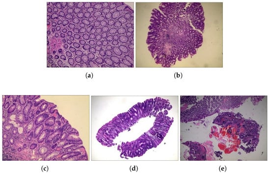
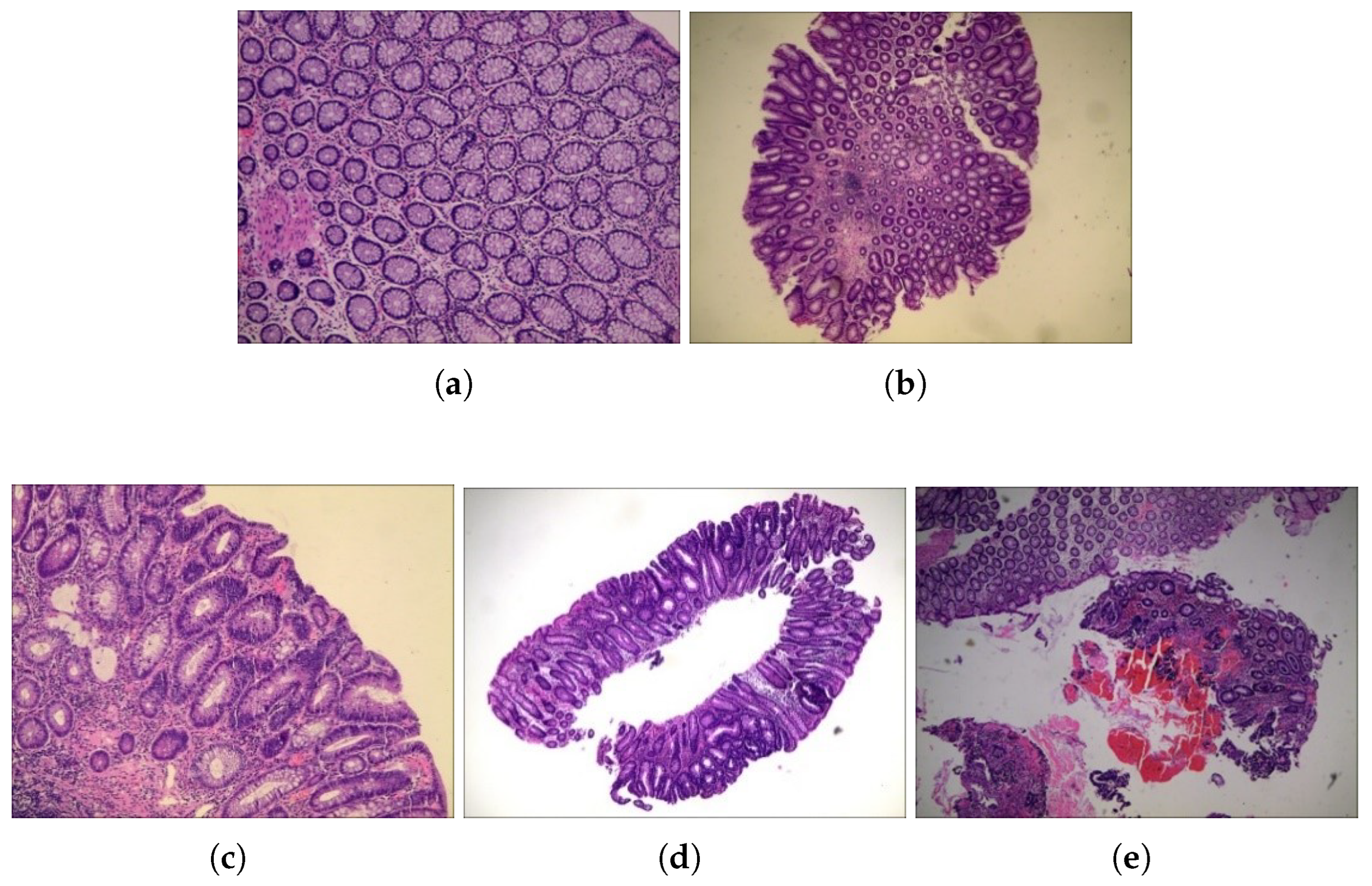
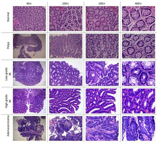
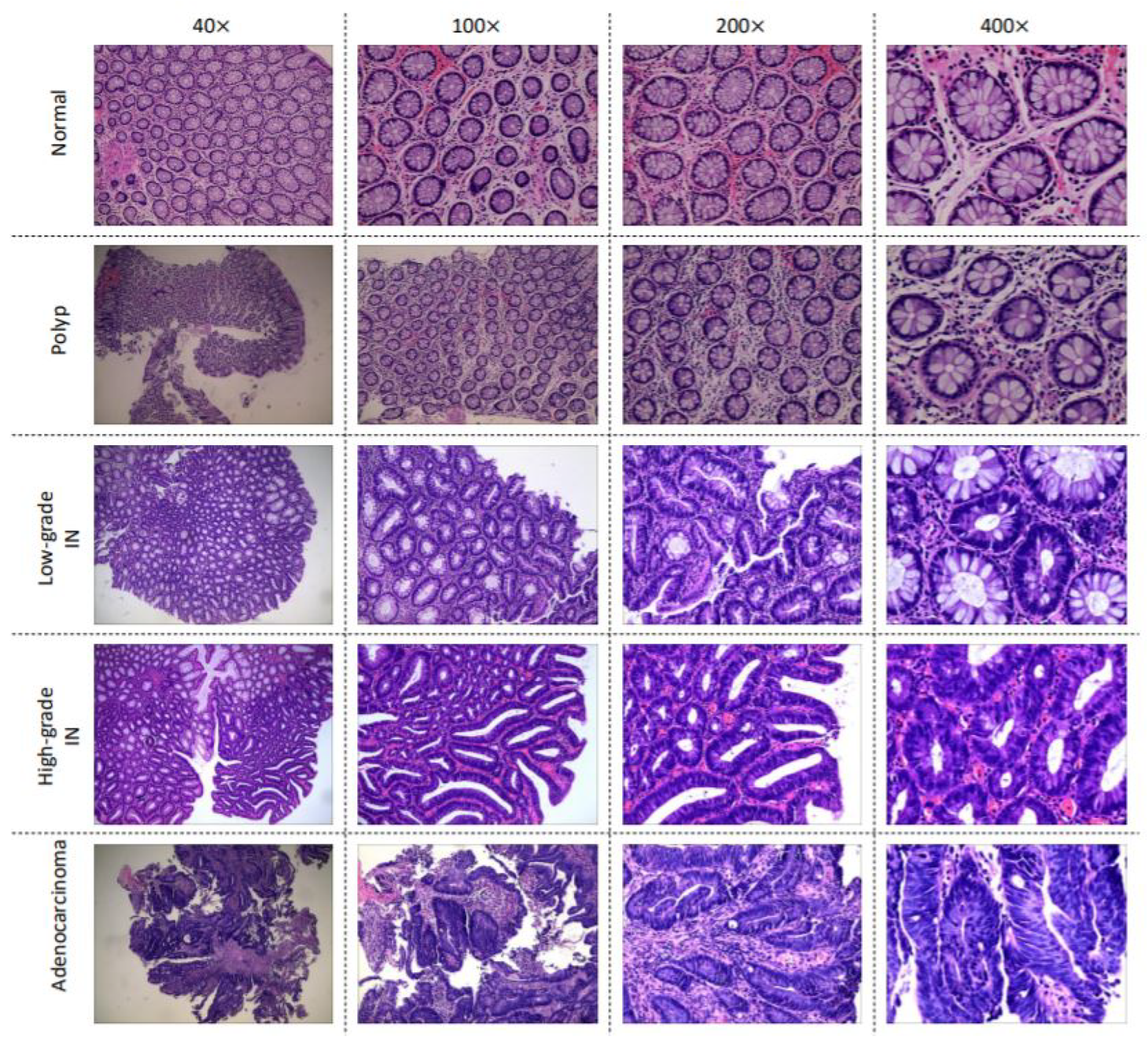
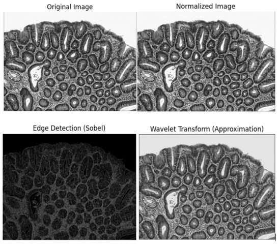
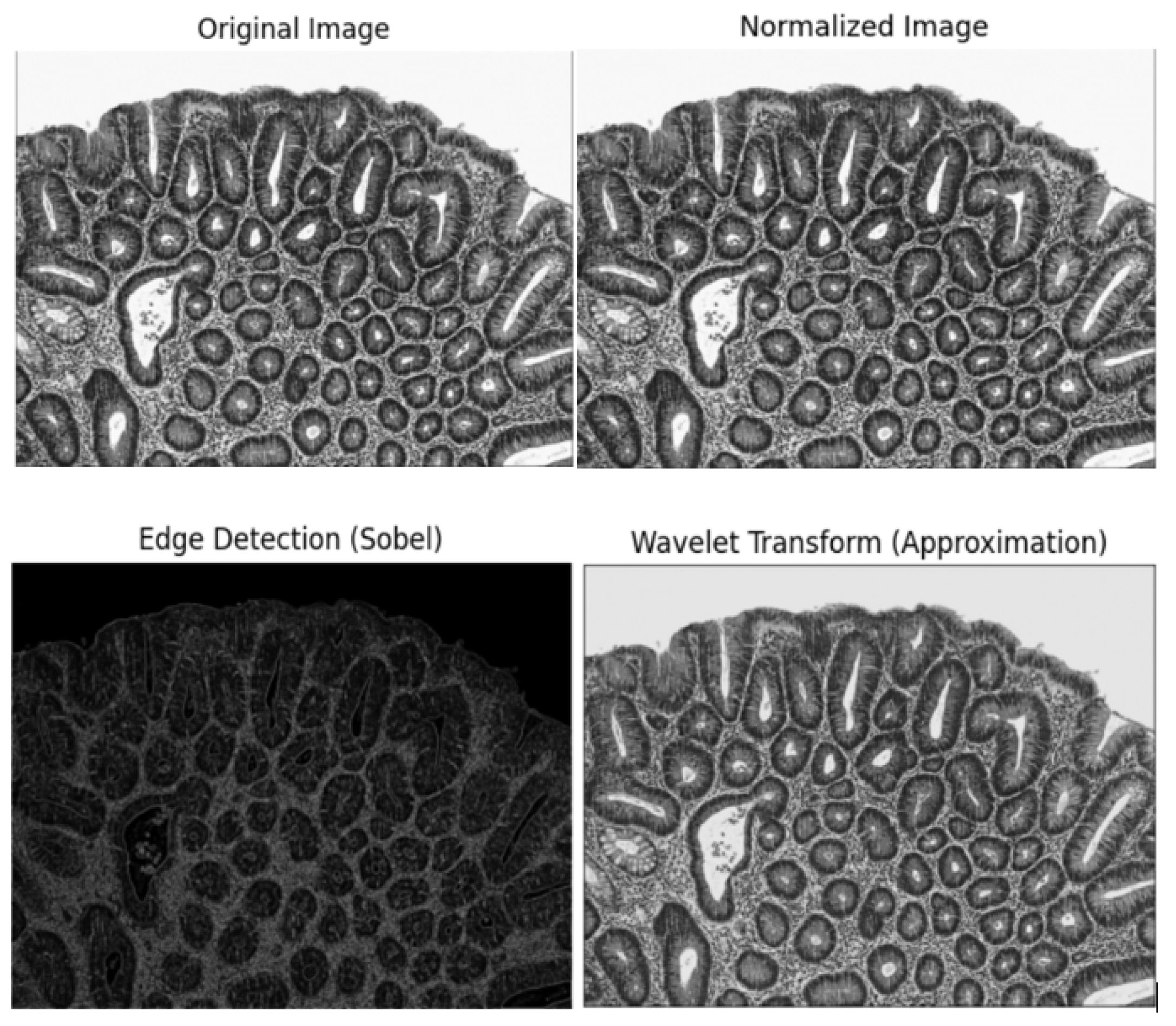
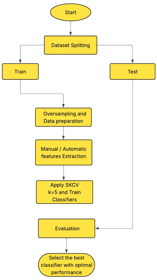
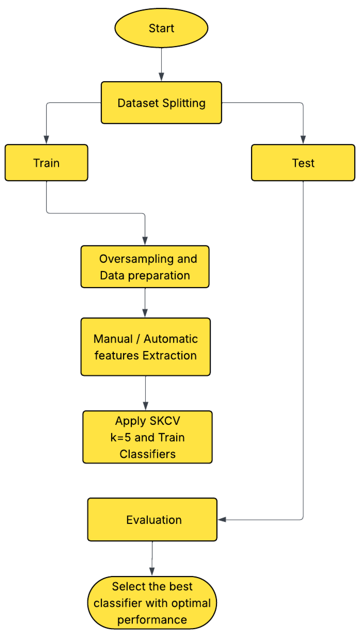
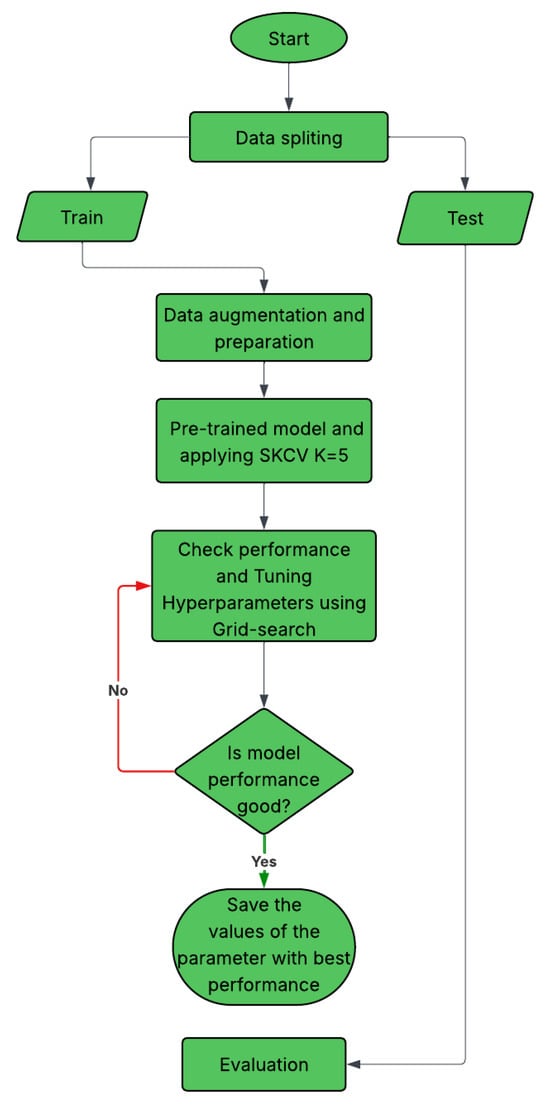
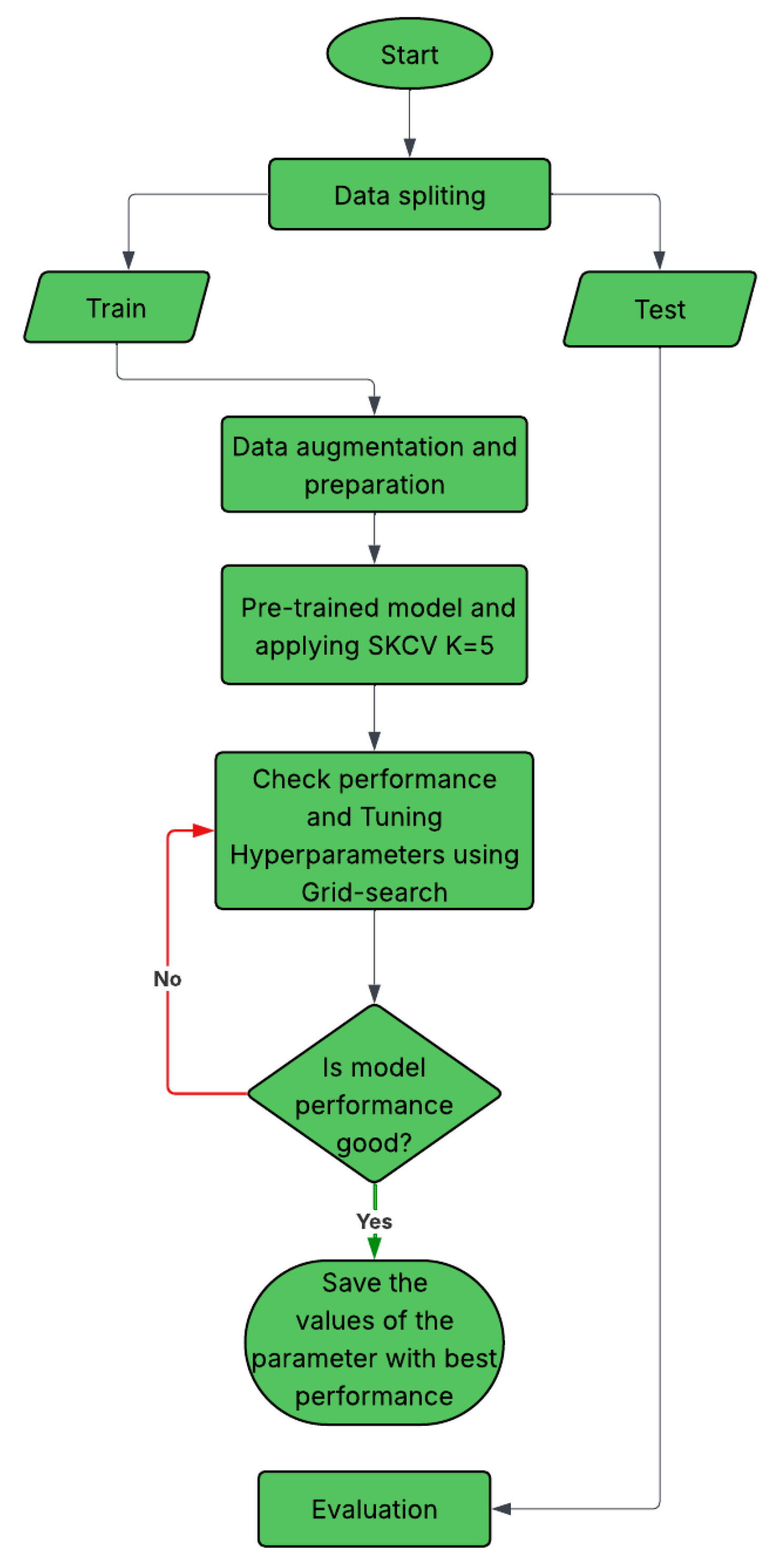
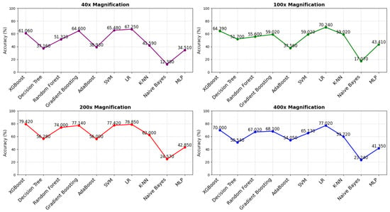
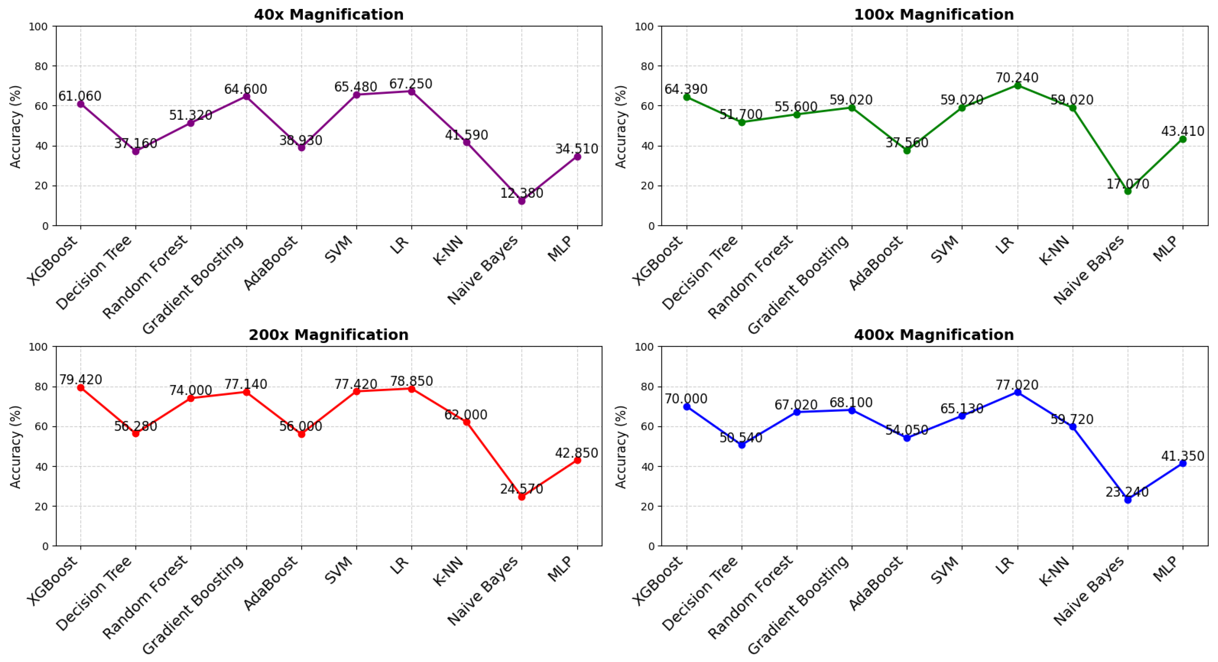
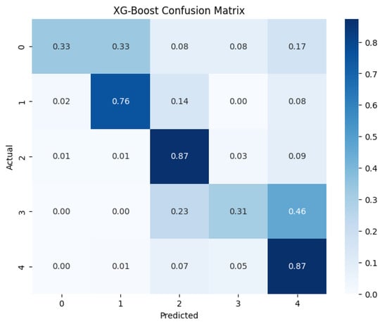
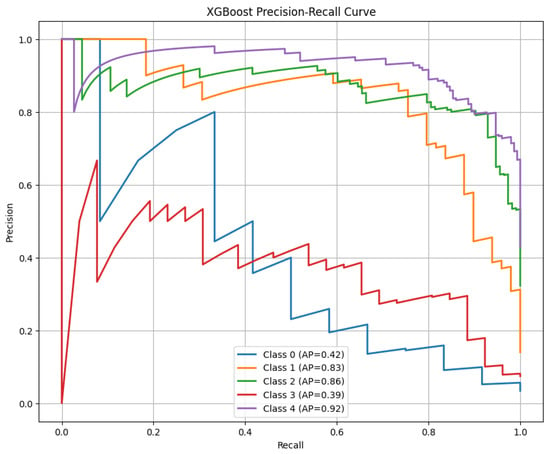
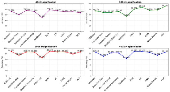
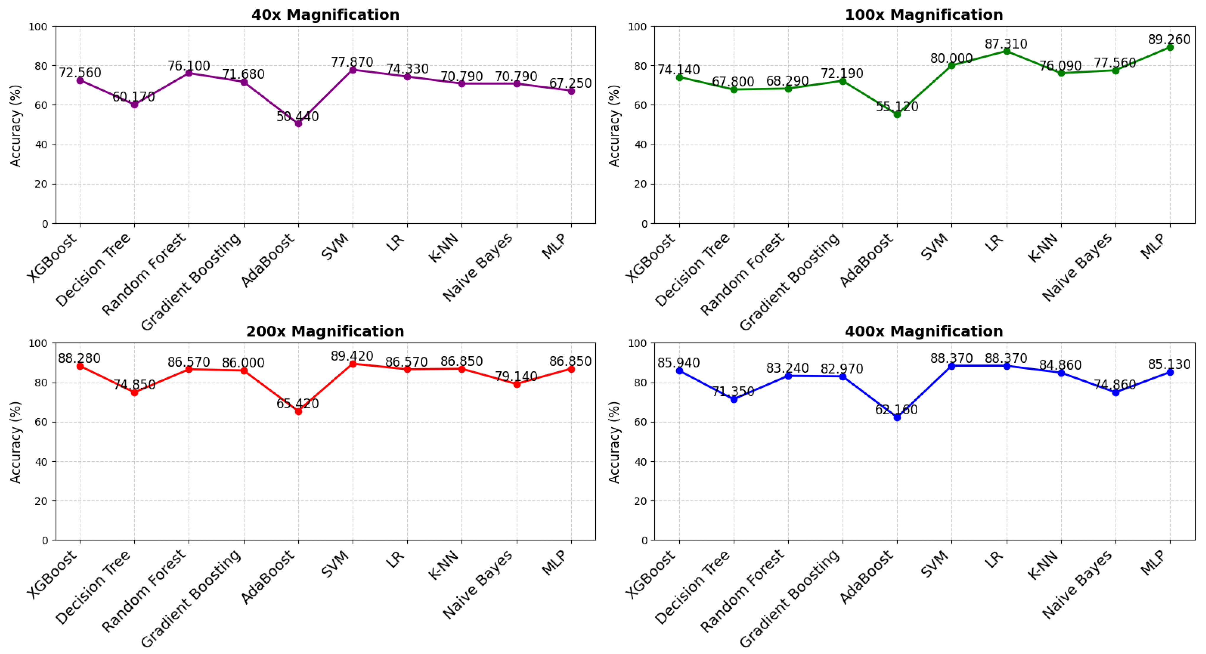
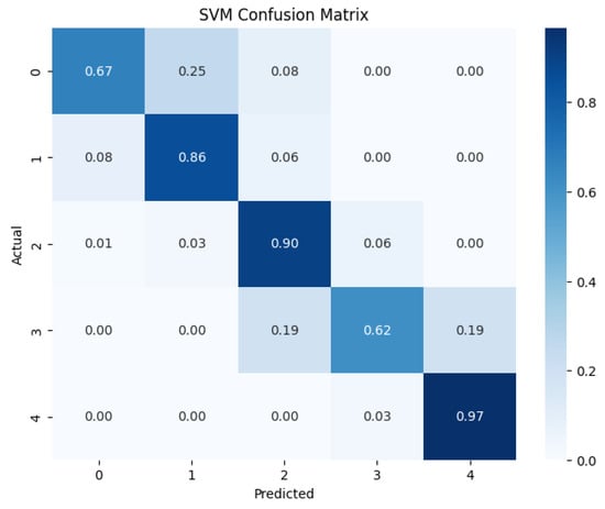
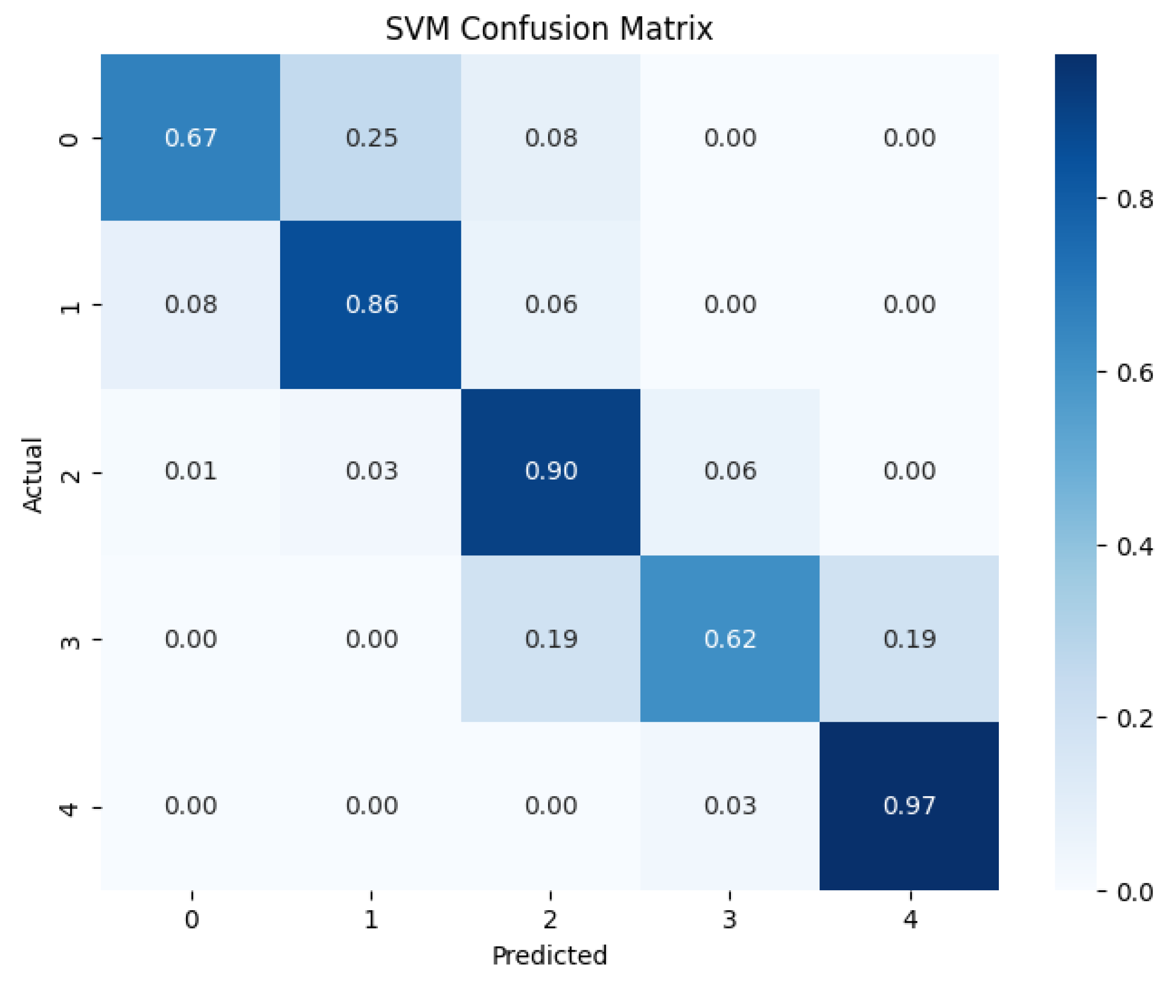
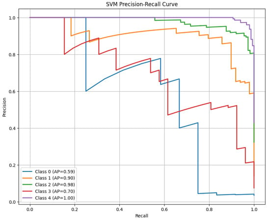
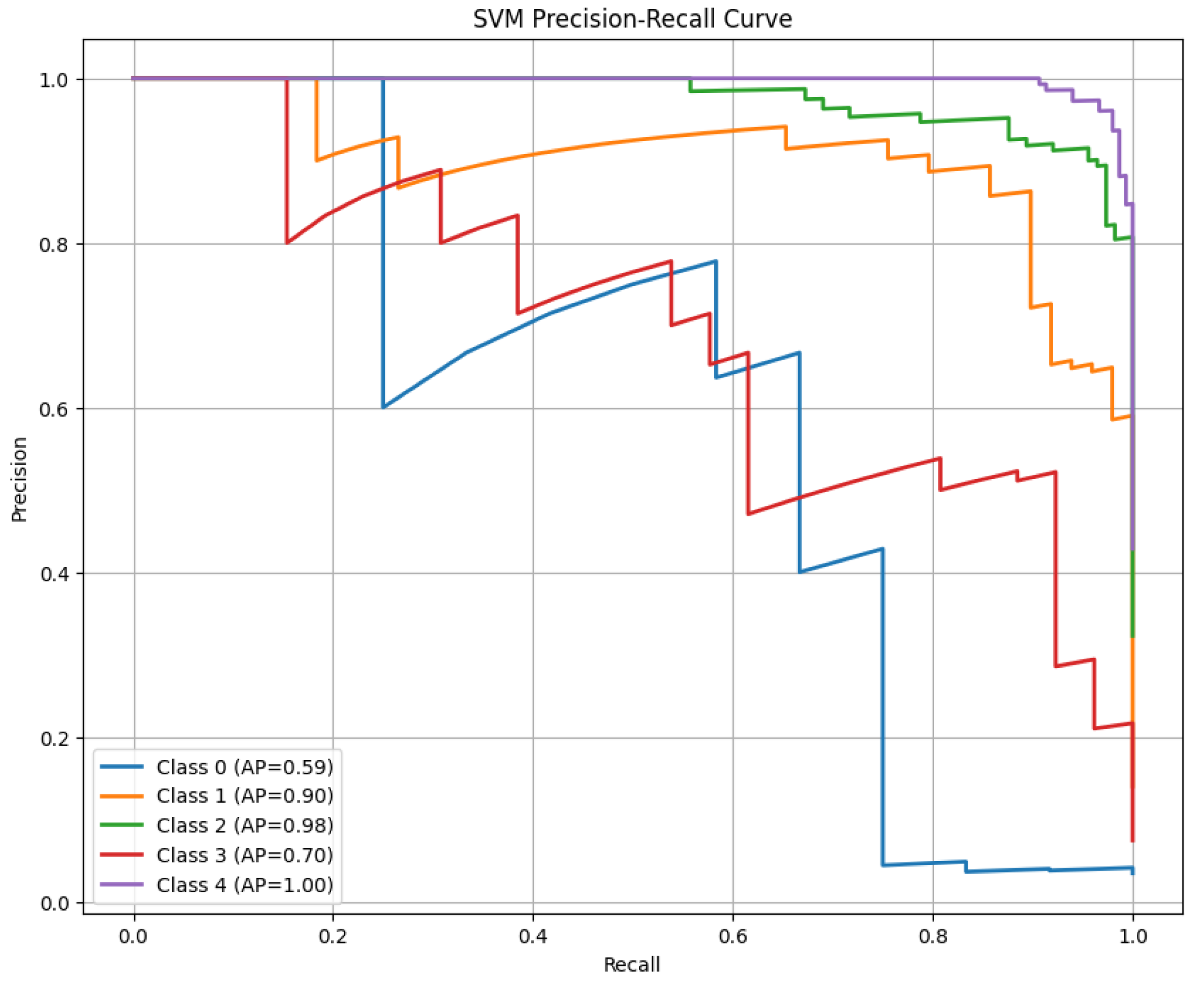
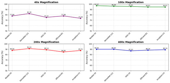
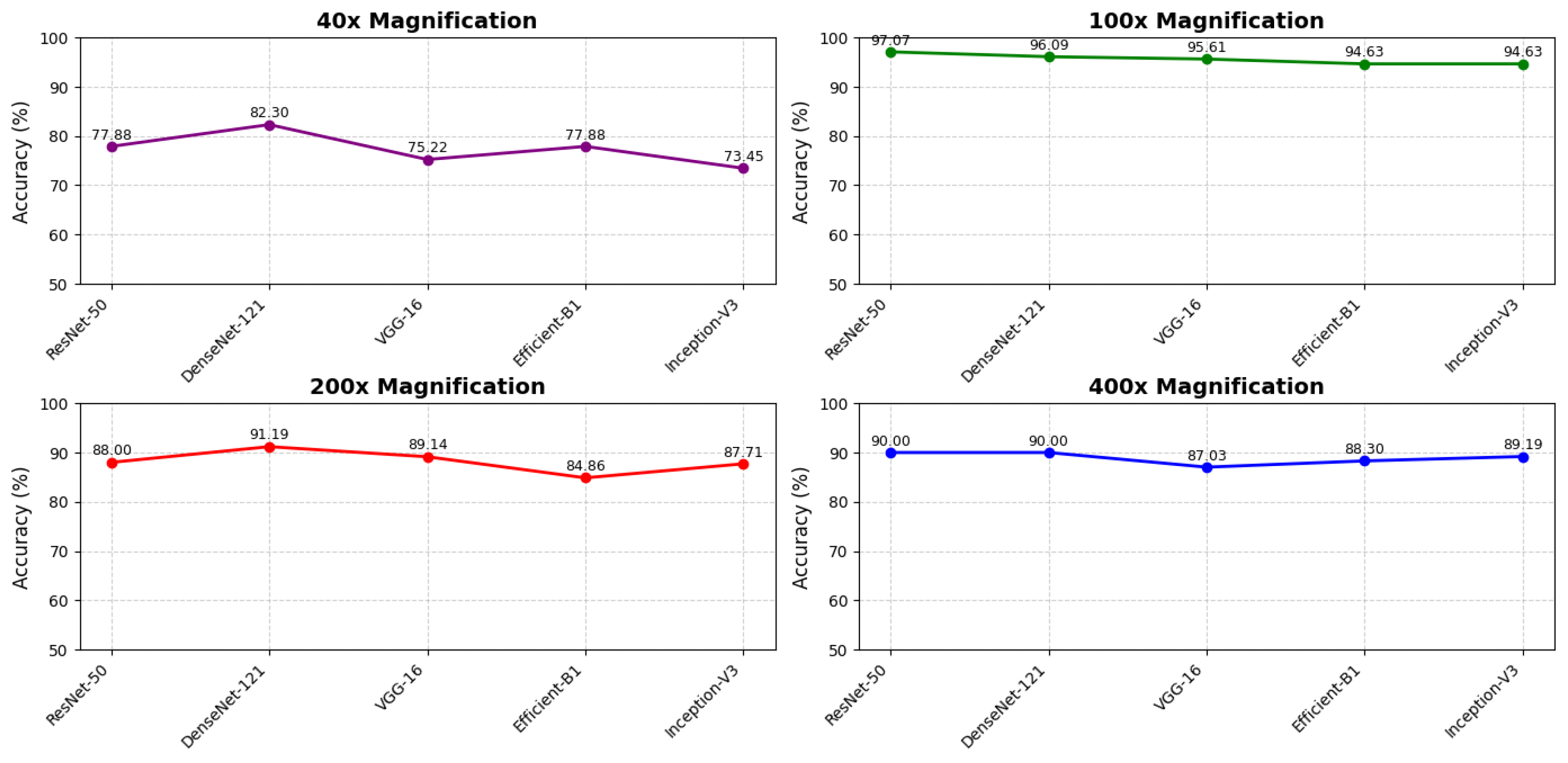
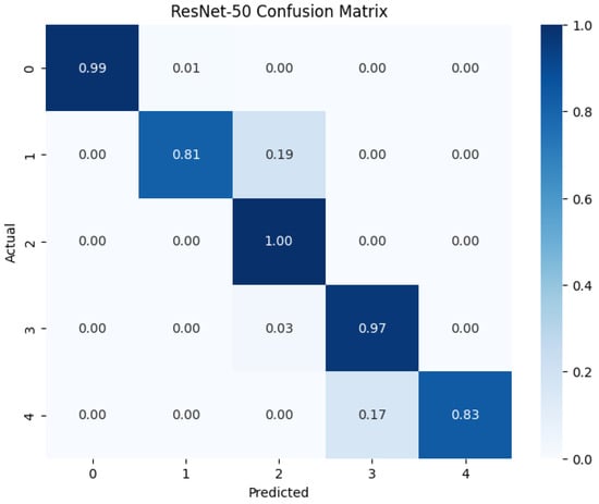
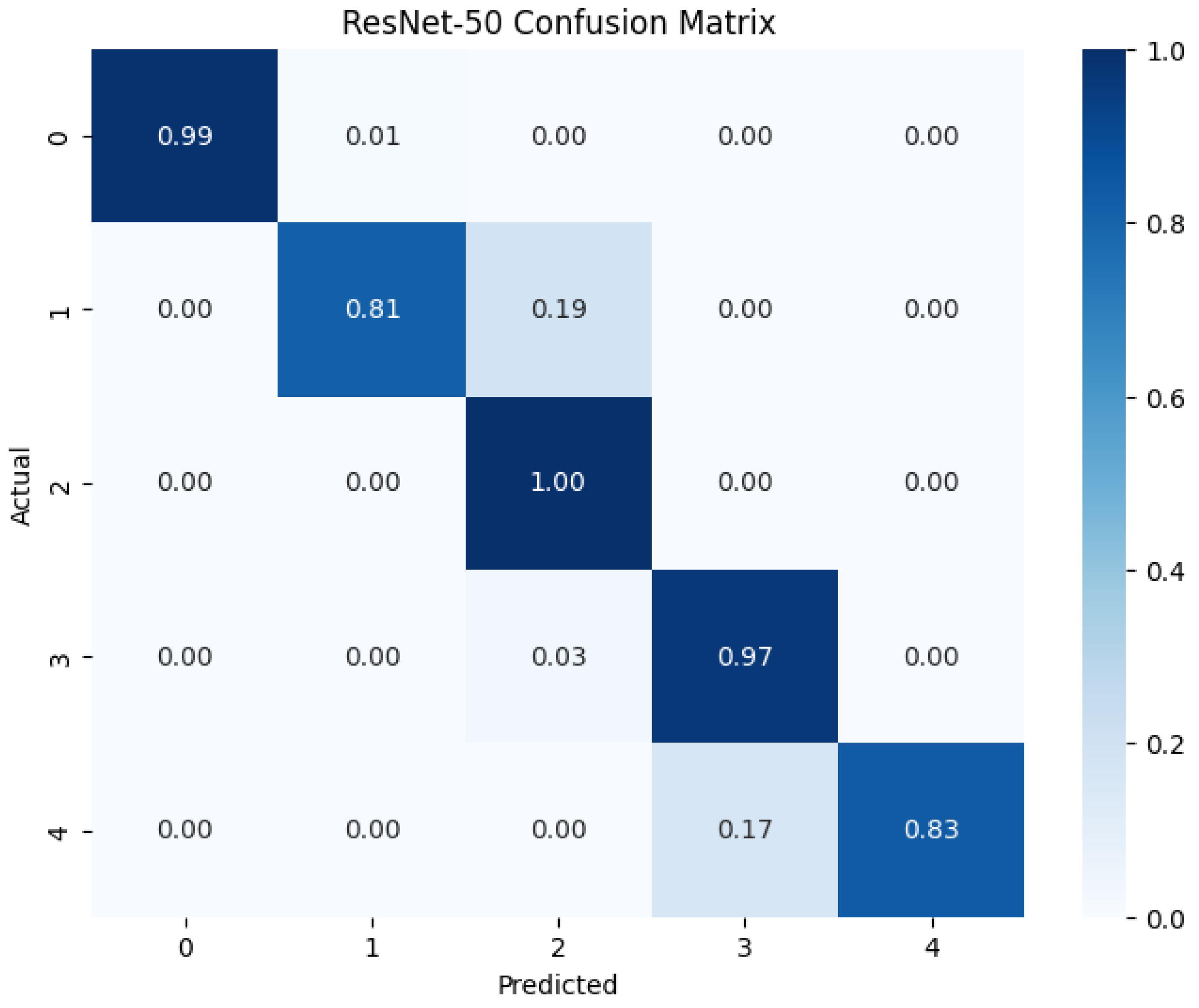
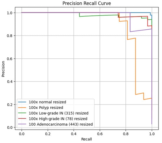
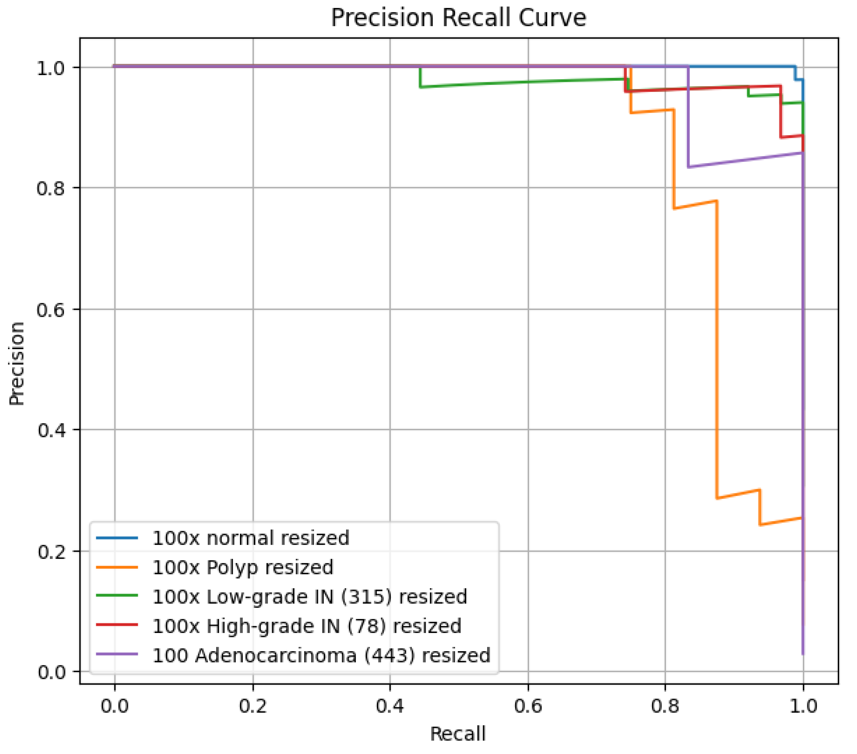
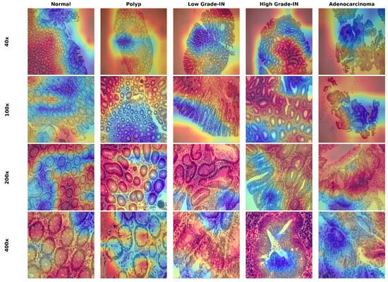
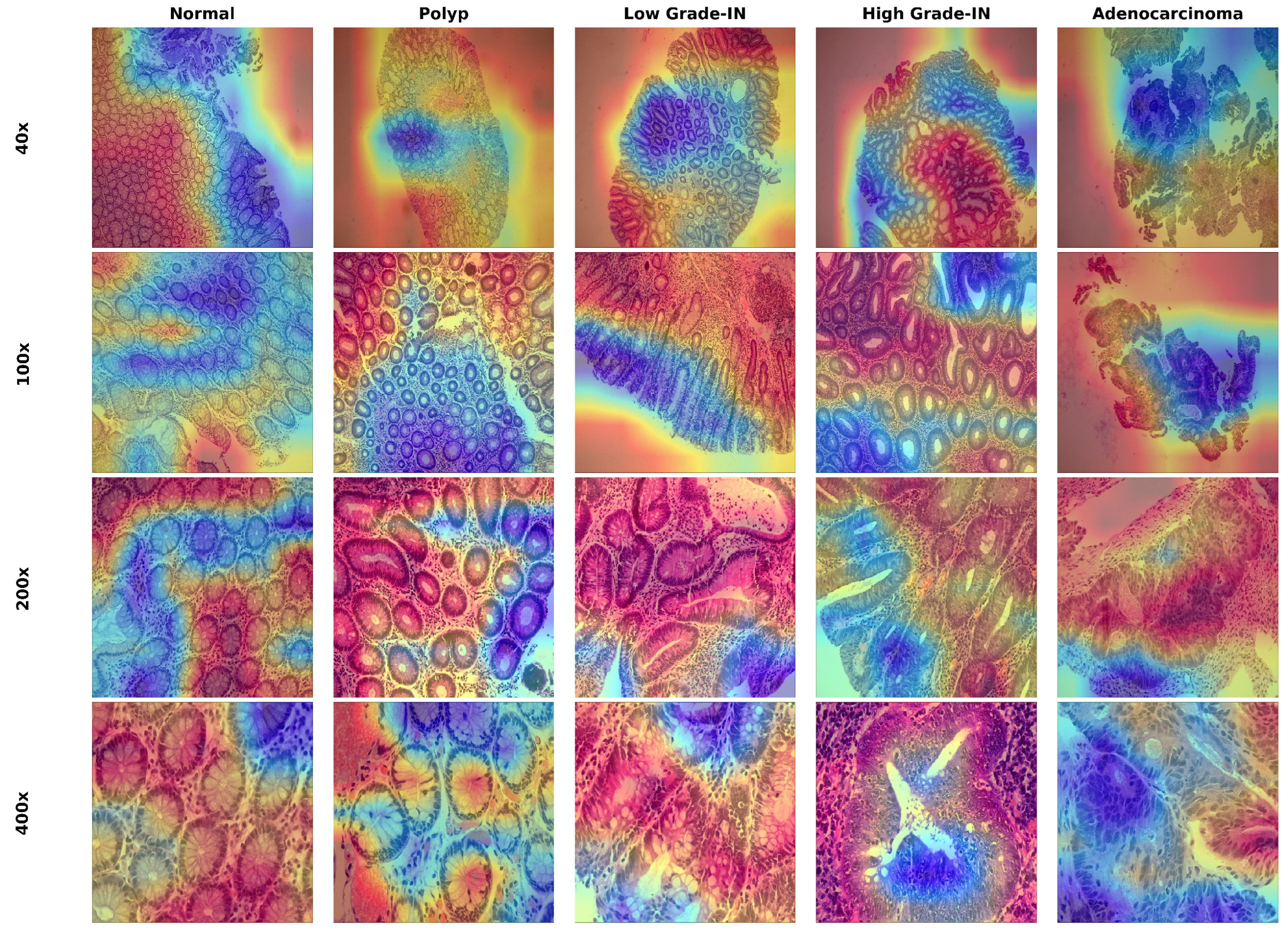

Disclaimer/Publisher’s Note: The statements, opinions and data contained in all publications are solely those of the individual author(s) and contributor(s) and not of MDPI and/or the editor(s). MDPI and/or the editor(s) disclaim responsibility for any injury to people or property resulting from any ideas, methods, instructions or products referred to in the content. |
© 2026 by the authors. Licensee MDPI, Basel, Switzerland. This article is an open access article distributed under the terms and conditions of the Creative Commons Attribution (CC BY) license.