Comparative Analysis of Spectrogram-Based Transformations for Acoustic Classification of SMAW Weld Quality Using Machine Learning

Abstract

This study evaluates the feasibility of acoustic signal analysis using different spectrographic transformation methods as a tool for assessing the quality of welding beads produced through the Shielded Metal Arc Welding (SMAW) process. Acoustic emissions were recorded during manual welding operations under controlled experimental conditions, using E6013 electrodes on A36 carbon steel plates. From the acoustic recordings of 400 welding samples, previously classified as accepted or rejected, two fundamental acoustic descriptors were extracted: the fundamental frequency (F₀) and the harmonic-to-noise ratio (HNR). These were analysed using parametric and non-parametric metrics to evaluate their discriminative capability. In addition, multiple supervised classifiers were trained and validated using stratified eight-fold cross-validation. The proposed framework enables a systematic comparison of different signal transformations and classification models for the evaluation of SMAW welding quality. Among the evaluated models (SVC, Gradient Boosting, and Extra Trees), precision rates of 90–95% were observed using Spectral Contrast, MEL, and CQT transformations. The results demonstrate that the implementation of various acoustic signal-based models and transformations for welding inspection offers a scalable and cost-effective solution for industrial quality control.

1. Introduction

Different industrial sectors have increasingly promoted intelligent mechanisms, such as artificial intelligence (AI) and machine learning (ML), with the aim of improving efficiency in industrial production [1]. These technologies have been integrated into modern manufacturing systems with high versatility, leading to a substantial transformation in industrial quality control strategies through the modelling of non-linear relationships, complex pattern classification, and process parameter optimisation [2,3]. Such approaches have been widely applied in predictive maintenance, early fault detection, process optimisation, automated quality inspection, and real-time data-driven decision-making [4,5,6]. Within this framework, joining and welding processes represent a field of particular interest due to their critical importance for the structural integrity of industrial components in sectors such as construction, automotive manufacturing, and energy production [7,8].

In modern manufacturing environments, machine learning techniques are increasingly used to support quality monitoring, predictive maintenance, and process optimization. Several studies have highlighted the growing role of artificial intelligence in Industry 4.0 for analysing complex process data and improving manufacturing decision-making [1,2,4]. In welding processes, quality evaluation is particularly challenging because it depends on multiple interacting variables such as arc stability, material behaviour, and operator performance. Therefore, monitoring techniques capable of capturing process dynamics are essential for supporting reliable quality assessment. In this context, acoustic emissions generated during welding provide a potential source of information about the process behaviour, enabling the development of classification models that assist in the evaluation of welding conditions.

The quality of a welded joint is influenced by multiple factors, including thermal gradients, material composition, and welding parameters, which may lead to porosity, cracking, and lack of fusion, thereby compromising mechanical properties and causing catastrophic failures in demanding industrial applications. Human performance constitutes another key factor in this manufacturing process, as it depends on the welder’s skill, experience, fatigue level, and judgement, introducing substantial variability in critical parameters such as arc length, electrode angle, and travel speed, which increases the probability of welding defects [9,10]. However, the implementation of AI and ML in this context faces significant challenges, including the difficulty of acquiring labelled datasets representative of real working conditions and the need to develop robust models capable of generalising across variations in human error and environmental conditions [11]. The development of intelligent systems capable of interpreting subtle patterns, such as motor coordination, hand–eye stability, and acoustic cues, could enable standardised and reproducible assessments of manual welding performance, integrating human expertise into data-driven production systems [12,13].

Recent studies, such as that by Ji et al. [14], developed a real-time welding inspection system based on a hybrid Squeeze-and-Excitation Convolutional Neural Network (SeCNN)-Long Short-Term Memory (LSTM) model, evaluated for robotic weld bead defect classification tasks, achieving an accuracy of 91.0% on the test dataset. In their investigation, acoustic signals were transformed into time–frequency representations, which served as inputs for the proposed model. Although the system outperformed comparative approaches such as CNN–SVM (83.7%) and CNN–BiLSTM (78.3%), the authors reported susceptibility to acoustic interference. Moreover, alternative time–frequency representations and applicability to highly variable manual processes, such as SMAW welding, were not explored.

On the other hand, Sumesh et al. [15] conducted a study on manual SMAW welding, focusing on the correlation between the acoustic signature of the arc and weld bead quality, which was classified into three conditions (sound weld, lack of fusion, and burn-through). The authors employed machine learning techniques such as Random Forest (RF) and J48 using AWS E6013 electrodes on carbon steel plates. The latter algorithm (J48) was specifically designed to enhance class separation through entropy-based decision rules, thereby reducing classification uncertainty. The results showed that the RF model achieved an accuracy of 88.7%, whereas J48 reached only 70.7%, highlighting a pronounced sensitivity of performance to algorithm selection. Although the study confirmed that arc sound contains sufficient information to discriminate between acceptable and defective welds, the authors emphasised the need to incorporate advanced signal processing procedures to filter unwanted noise during operation in order to improve model resolution.

In further developments, Koal et al. [16] investigated quality monitoring in industrial projection welding processes by analysing airborne sound captured using condenser microphones and applying ML techniques for process feature classification. The acoustic signals were processed using Fast Fourier Transform (FFT) to evaluate variations induced by handling errors and material differences. Subsequently, several models, including RF and XGBoost, were trained. Based on 300 experiments with five material variations, the proposed models achieved classification accuracies of up to 98.3% under controlled conditions, with F1-scores and areas under the ROC curve exceeding 0.99. Nevertheless, the authors reported a performance reduction of approximately 4% when omitting a microphone channel, highlighting the importance of acoustic signal enhancement for predictive accuracy.

Schmidt et al. [17] focused on acoustic monitoring in laser welding processes by employing a high-speed camera (10,000 frames·s⁻¹) inclined at 60° relative to the base plate surface, a narrow-band optical filter, an 808 nm laser system, and a high-precision balance to measure material loss. Using convolutional neural networks (CNNs) applied to acoustic emission signals, they identified transient events such as spatter and anomalies associated with welding parameters, including travel speed, focal position, and penetration depth. Their approach achieved prediction rates exceeding 90% for defective states, outperforming conventional spectral analysis methods. The authors highlighted the necessity of larger datasets to further improve acoustic-based quality control resolution.

Zhou et al. [18] developed an advanced laser welding penetration monitoring system based on acoustic emission analysis using a time–frequency representation derived from Variational Mode Decomposition (VMD) and a hybrid CNN–LSTM model. In their methodology, the signals were decomposed into nine intrinsic modes with distinct spectral content, enabling the isolation of components associated with physical phenomena such as molten pool dynamics and keyhole formation. These modes were subsequently transformed into time–frequency maps processed by CNNs, while LSTM networks modelled temporal dependencies. The proposed system achieved a classification accuracy of 99.8% for complete, partial, and unstable penetration states.

Although many studies have focused on implementing acoustic and time–frequency analysis for automated welding processes, predominantly based on laser, GMAW, and GTAW techniques, the systematic application of these methodologies to manual Shielded Metal Arc Welding (SMAW) has received considerably less attention. Most existing research relies primarily on Fourier-based transformations or related approaches to extract acoustic features and achieve predictive performance using methods such as wavelet analysis, CNN–LSTM models, and decision-tree-based classifiers. While these approaches have demonstrated promising results for specific welding configurations, they often focus on a single signal representation or feature extraction strategy. Consequently, limited attention has been given to systematically comparing different spectral transformations and evaluating how these representations influence classification performance in acoustic monitoring tasks, particularly in manual welding processes such as SMAW.

In this context, the contribution of this work is not the development of a new machine learning methodology but rather the systematic evaluation of different spectral signal representations for acoustic monitoring of manual SMAW welding processes. By analysing how various spectral and time–frequency transformations affect classification performance, this study aims to identify which representations provide the most informative acoustic features for weld quality assessment. From an application-oriented perspective, this analysis provides practical insights for the design of acoustic monitoring systems capable of supporting non-destructive evaluation of manual welding operations under realistic working conditions.

Within this context, the present study addresses this challenge by proposing an analysis focused on the application of different signal transformations to determine the optimal classification accuracy of a machine learning framework based on acoustic signal analysis for the non-destructive evaluation of manual SMAW weld quality. Field-recorded acoustic signals were transformed into time–frequency representations (spectrograms) that normalise signal duration while preserving temporal and spectral characteristics. A dataset comprising 400 welding records, including 200 acceptable and 200 defective weld beads, evaluated according to American Welding Society (AWS) criteria, was used to train and compare ten machine learning models for binary classification.

2. Materials and Methods

This section describes the experimental configuration, data acquisition system, data pre-processing procedures, and the signal processing pipeline adopted in this study. It details the welding conditions, acoustic recording system, pre-processing stages, and the construction of time–frequency representations used for feature extraction. In addition, this section outlines the machine learning models, training strategy, and evaluation metrics employed for weld quality classification.

2.1. Welding Materials

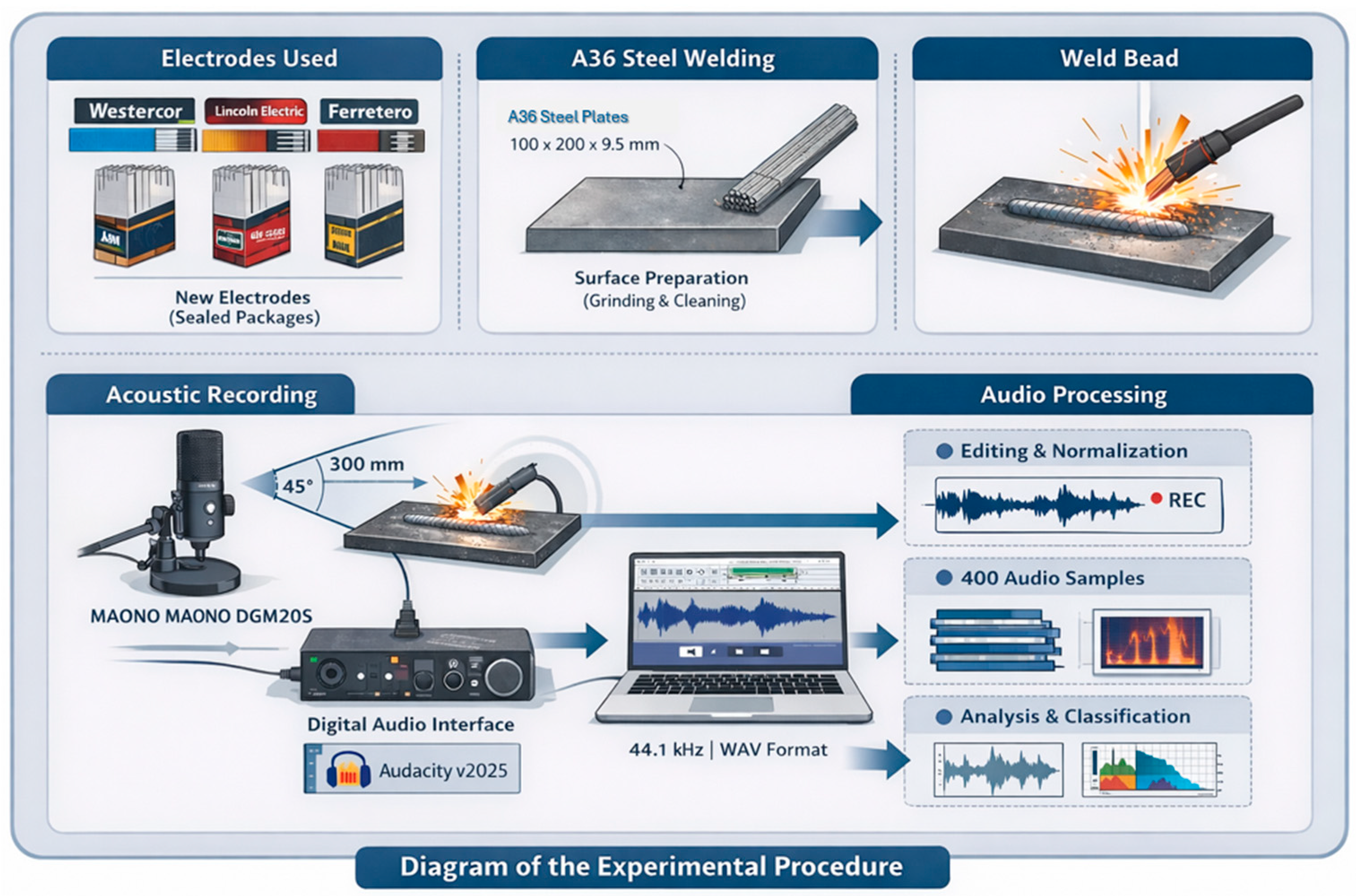
SMAW was performed using E6013 electrodes (1/8”) from three commercial manufacturers: Westercor (Bogotá, Colombia), Lincoln Electric (Cleveland, OH, USA), and Ferretero (Bogotá, Colombia). All electrodes were kept sealed prior to use to ensure consistent moisture content and coating conditions.

The base material consisted of low-carbon A36 structural steel plates (Local supplier, Bogota, Colombia) with dimensions of 100 mm × 200 mm × 9.5 mm (3/8”). Prior to experimentation, the plates were mechanically cleaned using a wire brush and subsequently degreased with acetone to remove oxides, scale, and surface contaminants that could affect welding performance.

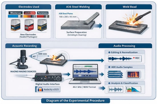
A total of 400 weld beads were deposited and inspected by a certified welder in accordance with the guidelines specified in the Welding Handbook, Volume I: Welding Science and Technology, published by the American Welding Society (AWS). Figure 1 illustrates the experimental configuration of the study.

2.2. Weld Bead Classification

The weld beads were produced using a Lincoln Electric Speedtec 200C multipurpose inverter welding system (Lincoln Electric, Cleveland, OH, USA). Based on the welder’s expertise, ten different test conditions were established, with current values ranging from 70 to 130 A and voltage levels between 22 and 30 V.

To ensure experimental traceability, the operational variables associated with each welding trial were systematically documented. In addition, alphanumeric codes were assigned to each weld bead, integrating information regarding the welder, applied current level, and corresponding quality category. Welds were classified as defective (0) or acceptable (1) in accordance with the criteria specified in Welding Handbook, Volume I: Welding Science and Technology (AWS).

During data acquisition, specific measures were implemented to reduce environmental acoustic interference and preserve the integrity of the recorded signals.

2.3. Acoustic Data Acquisition

The acoustic emissions generated during the experimental process were recorded using a MAONO DGM20S condenser microphone (MAONO Technology Co., Ltd., Shenzhen, China) equipped with an active noise reduction system. The sensor was positioned at an approximate distance of 300 mm from the electric arc and oriented at an angle of 45° with respect to the longitudinal axis of the weld bead in order to minimise electromagnetic interference.

The microphone was connected to a digital audio interface, and the signals were acquired using Audacity v2025 software at a sampling frequency of 44.1 kHz, with a 16-bit resolution on the microphone channel. All recordings were stored in WAV format.

Each welding operation was documented independently. Subsequently, the audio files were subjected to temporal segmentation and amplitude normalisation. A total of 400 acoustic signals were selected for further analysis.

2.4. Signal Processing and Image Generation

The recorded acoustic signals were transformed into visual spectrogram representations using the Python 3.10 environment, with the specialised libraries Librosa 0.11.0 and Matplotlib 3.10.8.

Acoustic feature extraction was performed using multiple spectral and time–frequency representations. Although several transformations rely internally on Short-Time Fourier Transform (STFT), the STFT spectrogram itself was not used as an independent representation in the analysis. Instead, STFT was only employed as an intermediate computational step required by several spectral descriptors implemented in the Librosa library. The study focused on higher-level spectral representations such as Mel spectrograms, MFCCs, spectral contrast, chromagrams, and other spectral descriptors, which provide more compact and discriminative representations of the welding arc sound. The parameter configuration used for each transformation is summarized in

Table 1. Parameters of each signal transformation applied to the tested weld beads.

Transformation	n_fft	Hop Length	Window	Specific Parameters	Notes
Mel Spectrogram	2048	512	Hann	n_mels = 128	Based on STFT decomposition
MFCC	2048	512	Hann	n_mfcc = 20, Mel bands = 128	Derived from Mel spectrogram
Constant-Q Transform (CQT)	—	512	Hann	n_bins = 84, bins_per_octave = 12	Logarithmic frequency resolution
Chromagram	2048	512	Hann	n_chroma = 12	Derived from STFT energy distribution
Tonnetz	—	—	—	6 tonal centroid dimensions	Computed from chroma features
Spectral Contrast	2048	512	Hann	n_bands = 6, quantile = 0.02	Spectral peak-valley analysis
Spectral Centroid	2048	512	Hann	—	Energy-weighted frequency center
Spectral Rolloff	2048	512	Hann	roll_percent = 0.85	Frequency containing 85% energy

to ensure reproducibility of the feature extraction process.

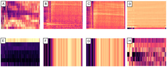
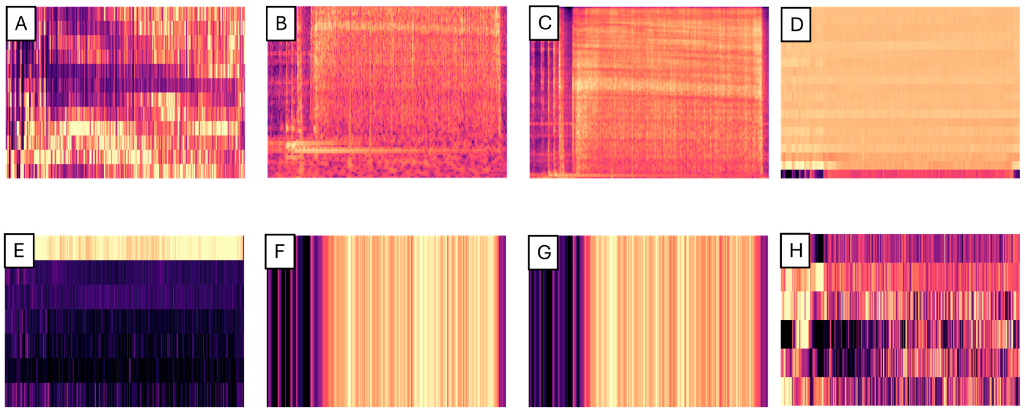
The images obtained from each transformation were saved in .WAV format to prevent any loss of quality. As shown in Figure 2, an example of the resulting spectrograms corresponding to an experimental weld bead is presented.

2.5. Statistical Analysis

The statistical comparison between the spectral metrics corresponding to the welding classification types was conducted using both parametric and non-parametric approaches, depending on the fulfilment of normality and homogeneity of variance assumptions.

For the evaluation of normality, the Anderson–Darling and Shapiro–Wilk tests were applied, chosen for their sensitivity to deviations in the tails of the distribution and their robustness with small- to medium-sized samples. However, as the analysis was based on a global matrix aggregated by transformation and class, the effective sample size per group was limited, reducing the sensitivity of the tests. Consequently, the analysis relied primarily on non-parametric procedures.

Homogeneity of variances across groups was assessed using Levene’s test (α = 0.05). In cases where these assumptions were not met, the Kruskal–Wallis test was employed as an alternative to analysis of variance (ANOVA).

Multiple comparisons between classifications were performed using Dunn’s post hoc test with Bonferroni adjustment to control the Type I error rate. All statistical analyses were implemented in the Python environment (v3.10), utilising the SciPy, Statsmodels, and Scikit-posthoc libraries. Differences were considered statistically significant at a 95% confidence level (p < 0.05).

2.6. Machine Learning Models

A stratified 10-fold cross-validation scheme was employed to evaluate the performance of all spectrogram-based classifiers. This procedure was implemented using the StratifiedKFold function from the scikit-learn library, configured with ten folds, enabled randomisation, and a fixed seed (42) to ensure reproducibility of the results.

For each iteration, nine folds were used to train the models, while the remaining fold was reserved for validation. This strategy preserved the original balance of welding classifications across all classes. Notably, an independent hold-out test set was not defined due to the sample size; therefore, stratified cross-validation was adopted as the primary estimator of generalisation performance. To prevent data leakage, all preprocessing steps, including feature scaling, were integrated within scikit-learn Pipeline objects alongside each classifier.

The following machine learning algorithms were evaluated for classification: Support Vector Classifier (SVC), Logistic Regression (LR), Linear Support Vector Classifier (Linear SVC), Linear SVC with probabilistic calibration (L + C), Stochastic Gradient Classifier with calibration (S + C), K-Nearest Neighbors (KNN), Decision Trees (DT), Random Forest (RF), Extra Trees (ET), Gradient Boosting (GB), and Gaussian Naïve Bayes (NB). No data augmentation techniques were applied, and all models were trained and evaluated exclusively using the original experimental spectrograms.

Hyperparameter optimisation was performed using the Optuna library. For each classifier, predefined hyperparameter search spaces were explored to identify configurations that maximised both classification accuracy and F1-score. The optimisation process consisted of 100 to 250 trials depending on model complexity and was constrained to a maximum computation time of 14,400 s (4 h). Model performance during optimisation was evaluated using stratified 10-fold cross-validation. Convergence behaviour was monitored through optimisation history plots to ensure stability of the search process. The optimal hyperparameter configurations obtained for each classifier are reported in Appendix A.

2.7. Spectral Feature Extraction

In order to characterise the dynamic behaviour of the electric arc and the energy variations during the SMAW process, spectral equations based on entropy were applied to describe the spectrogram generated for each transformation.

2.7.1. Spectral Energy

This parameter quantifies the overall intensity of the acoustic phenomenon produced during welding. Using Parseval’s theorem (Equation (1)), it is established that the total energy computed in the time domain must be equal to the total energy computed in the frequency domain. This represents a statement of energy conservation [19].

$${\int }_{-\infty }^{\infty }x\left(t\right)x\left(t\right)dt={\int }_{-\infty }^{\infty }{\left|x\left(f\right)\right|}^{2}df$$

(1)

Accordingly, the discrete form of Parseval’s theorem is defined from this formula (Equation (2)).

$${\sum }_{i=0}^{n-1}{\left|xi\right|}^2={\displaystyle \frac{1}{n}}{\sum }_{k=0}^{n-1}{\left|xk\right|}^2,$$

(2)

where xi and xk represent a pair from the discrete Fourier transform and n is the number of elements in the sequence.

2.7.2. Band Energy

This parameter allows for the measurement of how the energy of a signal is distributed across specific frequency intervals from point a to point b. It is calculated using Equation (3) by integrating the spectral energy density over the frequency band under study [19].

$${\int }_a^b{\left|x\left(f\right)\right|}^{2}df$$

(3)

2.7.3. Spectral Centroid

The spectral centroid is defined as a feature of the spectral set, calculated by weighting the frequencies and computing their mean, which helps to characterise the “brightness” of a sound wave. It is derived from the spectrogram of a sound wave generated via the Fourier transform, indicating that higher frequency components contribute to a brighter auditory perception [20]. Equation (4) is used for its calculation.

$$C={\displaystyle \frac{{\Sigma }_{i}s\left[k_i,t\right]\cdot f_r\left[k_i\right]}{{\Sigma }_{J}s\overline{\left[j,t\right]}}},$$

(4)

where $i$ and $j$ range from 0 to $n-1$, $t$ represents time in seconds, $n$ denotes the number of frequency values per second, $s$ corresponds to the spectrogram of the sound wave, and $f_r$ is the set of frequencies found in row $k$ of the spectrogram matrix [21].

2.7.4. Spectral Flatness

Spectral flatness is a measure commonly used in digital signal processing to characterise an audio spectrum. It is typically expressed in decibels and allows for quantifying the similarity of a sound to a pure tone as opposed to its similarity to noise [22]. It is calculated as the ratio of the geometric mean to the arithmetic mean of the power spectrum, as shown in Equation (5).

$$Sf\left(n\right)={\displaystyle \frac{\mathit{exp}\left(\frac{1}{N}{\sum }_{n=1}^{N-1}\mathit{ln}S\left(n\right)\right)}{\frac{1}{N}{\sum }_{n=1}^{N-1}S\left(n\right)}},$$

(5)

where $n$ represents the discrete values of the power spectrum and $N$ denotes the total number of spectral components.

The extraction of spectral metrics was motivated by the need to obtain a compact representation of the information contained in the spectrograms of the acoustic signals generated during the welding process. These metrics describe relevant properties of the spectrum, such as the distribution of energy and spectral structure, which are useful for characterizing differences between classes. Additionally, the use of spectral metrics contributes to reducing the dimensionality of the data without the need to train additional models or apply more complex dimensionality reduction techniques. In this way, the spectrogram information can be summarized through a set of meaningful descriptors that facilitate subsequent analysis and classification tasks.

3. Evaluation of Classification Models Under Spectral Transformations

The descriptive variables (mean, median, maximum and minimum values and standard deviation) were statistically analysed to determine whether significant differences existed between the transformations applied, taking into account their behaviour according to spectral type and welding bead classification.

For the evaluation of the machine learning classification models, metrics such as F1 score, accuracy, recall, and precision were applied at both macro levels to obtain a global assessment of system performance and micro levels to analyse the model’s specific behaviour for each welding quality class.

3.1. Comparative Statistical Analysis Between Transformations and Classes

As shown in

Table 2. Description of parameters by welding class distribution.

Parameter	Class	Count	Max	Mean	Min	Std	25%	50%	75%
Total Energy	1	1600	2.47	−0.01	−1.74	0.99	−0.75	0.03	0.54
	0	1688	2.20	0.01	−1.71	1.01	−0.72	0.03	0.52
Low-Band Energy	1	1600	2.90	−0.01	−2.38	1.00	−0.61	−0.00	0.47
	0	1688	2.43	0.01	−2.39	0.99	−0.57	0.02	0.35
Low–Mid-Band Energy	1	1600	2.35	−0.02	−1.91	1.00	−0.62	−0.02	0.58
	0	1688	2.03	0.02	−1.89	0.99	−0.49	−0.01	0.63
High–Mid-Band Energy	1	1600	2.25	−0.00	−2.01	0.98	−0.42	0.01	0.55
	0	1688	2.00	0.00	−1.99	1.01	−0.49	0.10	0.52
High-Band Energy	1	1600	1.71	0.01	−2.11	0.98	−0.40	0.14	0.66
	0	1688	1.69	−0.01	−2.11	1.01	−0.53	0.09	0.67
Spectral Centroid	1	1600	1.61	0.01	−2.76	1.01	0.18	0.33	0.48
	0	1688	1.50	−0.01	−2.75	0.98	0.18	0.29	0.474
Spectral Flatness	1	1600	0.95	0.01	−2.80	1.02	0.16	0.31	0.48
	0	1688	0.92	−0.01	−2.77	0.97	0.10	0.27	0.43

, the energy-based variables across the different frequency bands exhibit similar central values between classes, with means close to zero and medians around 0.03, indicating normalised distributions. However, the dispersion measures reveal relevant differences: low-band and low–mid-band energy present lower median values in defective welds (−0.004 and −0.027, respectively) compared to sound welds (0.021 and −0.005), suggesting reduced acoustic stability at lower frequencies.

The standard deviations remain close to 1.0, whereas high-band energy shows wide interquartile ranges, with 75th percentile values close to 0.67, indicating variability associated with arc instabilities and spatter events. Additionally, the spectral centroid and spectral flatness exhibit broader ranges, with centroid maxima exceeding 1.50 and flatness standard deviations above 1.02, reflecting their sensitivity to changes in arc dynamics and frequency behaviour during the SMAW process.

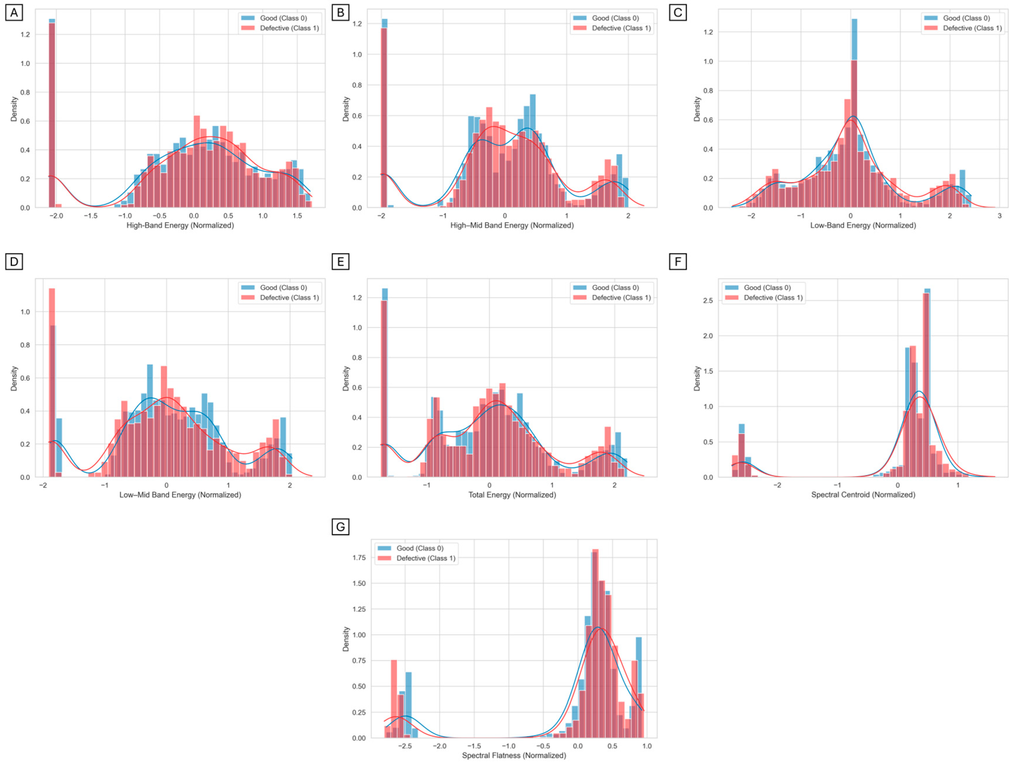
Figure 3 presents the distributions obtained from the acoustic signals, which exhibit differences in shape and dispersion between the welding classes. In the case of total energy, both classes show similar density peaks, with maximum values at around 0.35–0.40, indicating that these energy levels are the most frequent during bead deposition. For low-band and low–mid-band energy, Class 1 shows a higher density in negative ranges, with peaks between −0.5 and −0.3, whereas Class 0 displays a distribution shifted towards values closer to zero. In contrast, high-band and high–mid-band energy values show a concentration of defective samples at positive values, where the density of Class 1 reaches approximately 0.30–0.35 for energies above 0.40, accompanied by more extended right-hand tails.

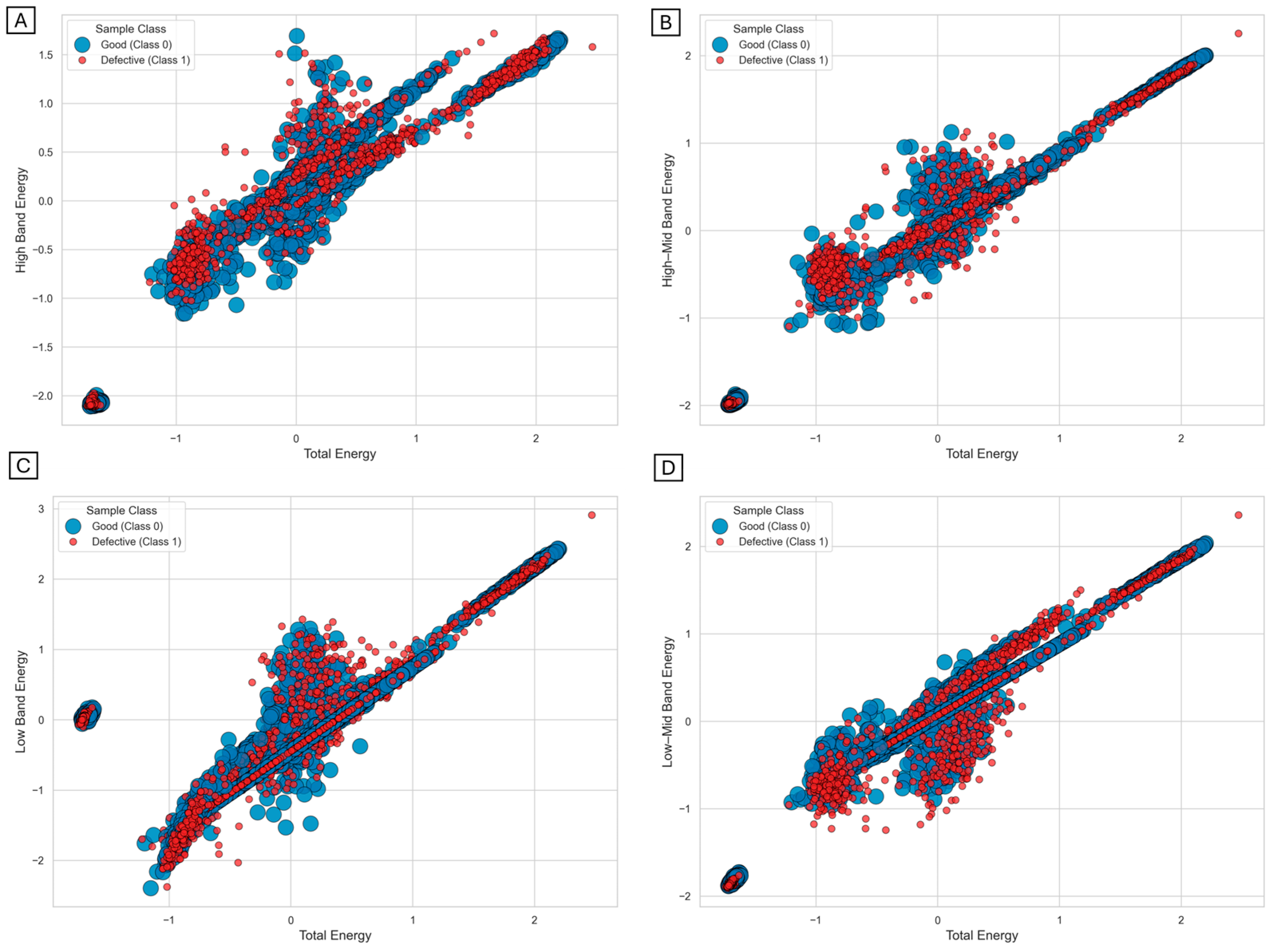
As a complement to the previous analysis, Figure 4 explores the relationships among the spectral energy descriptors through class-separated scatter plots. A strong positive linear dependence is observed between total energy and the energy contained in the different spectral bands. This behavior is expected because band energies represent partitions of the overall signal energy and therefore scale proportionally with the total acoustic power of the welding arc. Consequently, both acceptable and defective welds follow a similar global linear trend, which explains the significant class overlap observed in the plots.

Although the overall structure of the distributions is similar, defective weld beads exhibit noticeably greater dispersion around the main linear trajectory. This increased variability is consistent with the unstable behavior of the arc during defective welding conditions. In manual SMAW, irregular metal transfer, arc length fluctuations, and intermittent arc interruptions generate transient acoustic events that broaden the distribution of spectral energy. In contrast, acceptable weld beads tend to concentrate more closely along the linear energy trajectory, reflecting a more stable arc regime and a consistent energy distribution across the frequency bands.

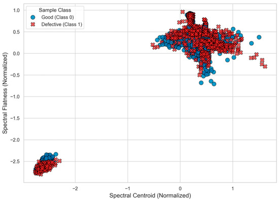
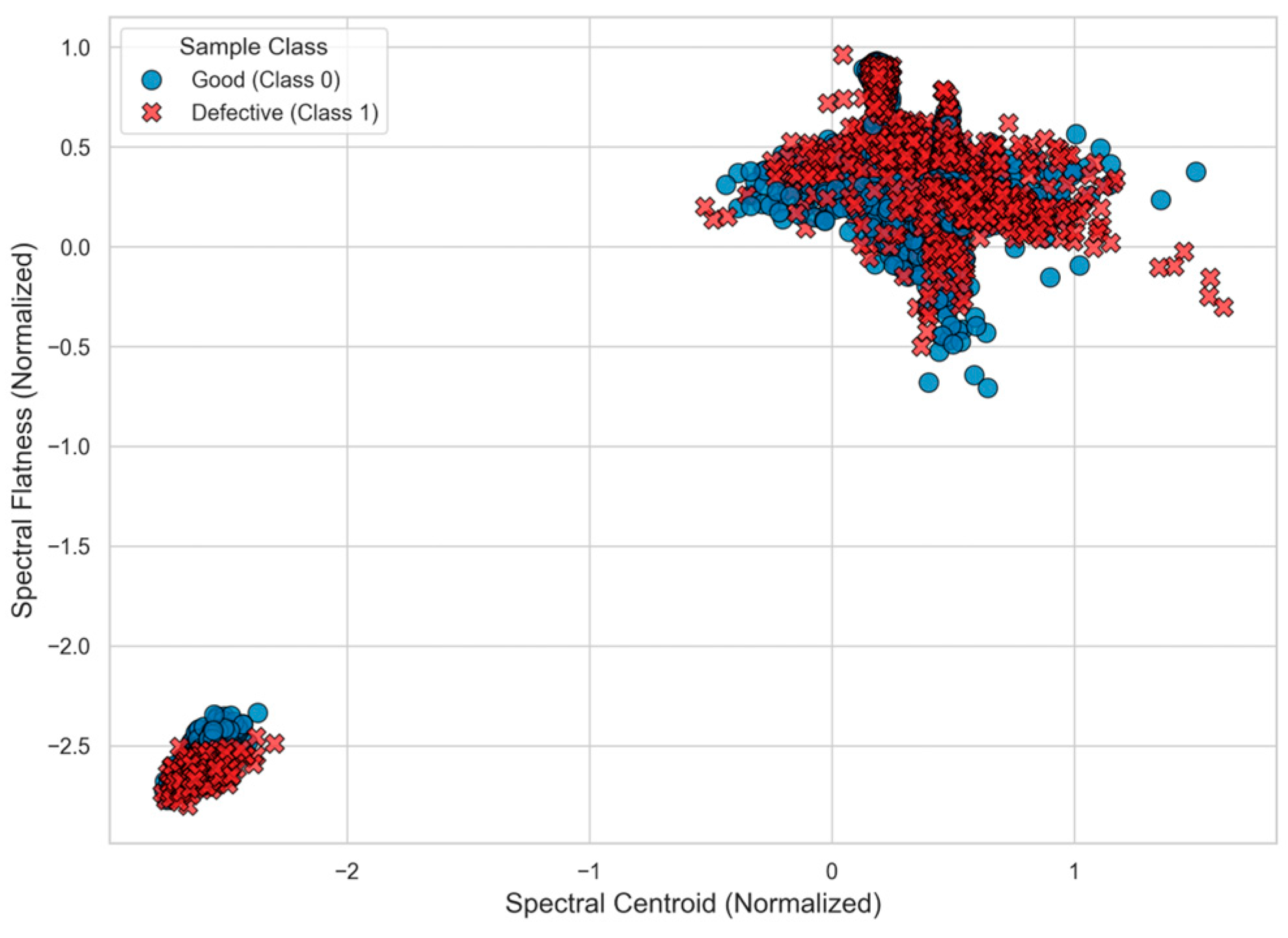
Figure 5 further examines the relationship between spectral centroid and spectral flatness. Two dominant regimes can be observed in the feature space, with substantial overlap between the two classes. This result indicates that these descriptors alone do not provide strong linear separability between acceptable and defective welds. However, defective welds present a higher dispersion in spectral flatness values, particularly at intermediate centroid levels. This behavior suggests the presence of broadband noise components associated with unstable arc dynamics and irregular droplet transfer.

Importantly, the purpose of these visualizations is not to demonstrate complete class separation using individual descriptors but rather to characterize the statistical structure of the acoustic features. The observed overlap confirms that the classification problem is inherently multidimensional and cannot be reliably solved using single spectral descriptors. Instead, discriminative information emerges from the combined interaction of multiple features, which explains why the machine learning models evaluated in this study achieve significantly higher classification performance when the descriptors are analyzed jointly.

The variations observed in the acoustic energy distributions, together with the partial overlap across certain energy ranges, indicate that visual discrimination between weld bead quality states is not trivial, thereby justifying the adoption of multivariate and machine learning (ML) approaches. It is important to highlight that the real welding process is inherently multifactorial, involving several operational variables associated with the Shielded Metal Arc Welding (SMAW) process, such as welding current, arc stability, electrode behaviour, and material interaction. In the present study, these input variables were not explicitly incorporated into the analysis. Instead, the proposed approach focuses on the spectral characteristics extracted from the acoustic emissions generated during the welding process. Consequently, the acoustic features analysed may implicitly reflect the combined influence of these operational factors, even though the process parameters themselves were not directly included as model inputs.

Consistent with this behaviour, normality and homoscedasticity tests revealed violations of parametric assumptions (p < 0.05). For this reason, the Kruskal–Wallis test was prioritised, confirming the existence of statistically significant differences among the spectral transformations (p = 0.0). Subsequently, these differences were further characterised through post hoc Bonferroni analysis, which enabled the identification of the most discriminative spectral representations. The underlying assumptions and non-parametric tests are detailed in Appendix B and Appendix C.

3.2. Distribution of Spectral Variables Across Transformations and Classes

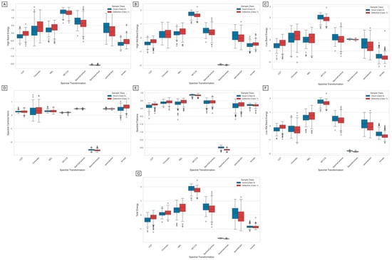
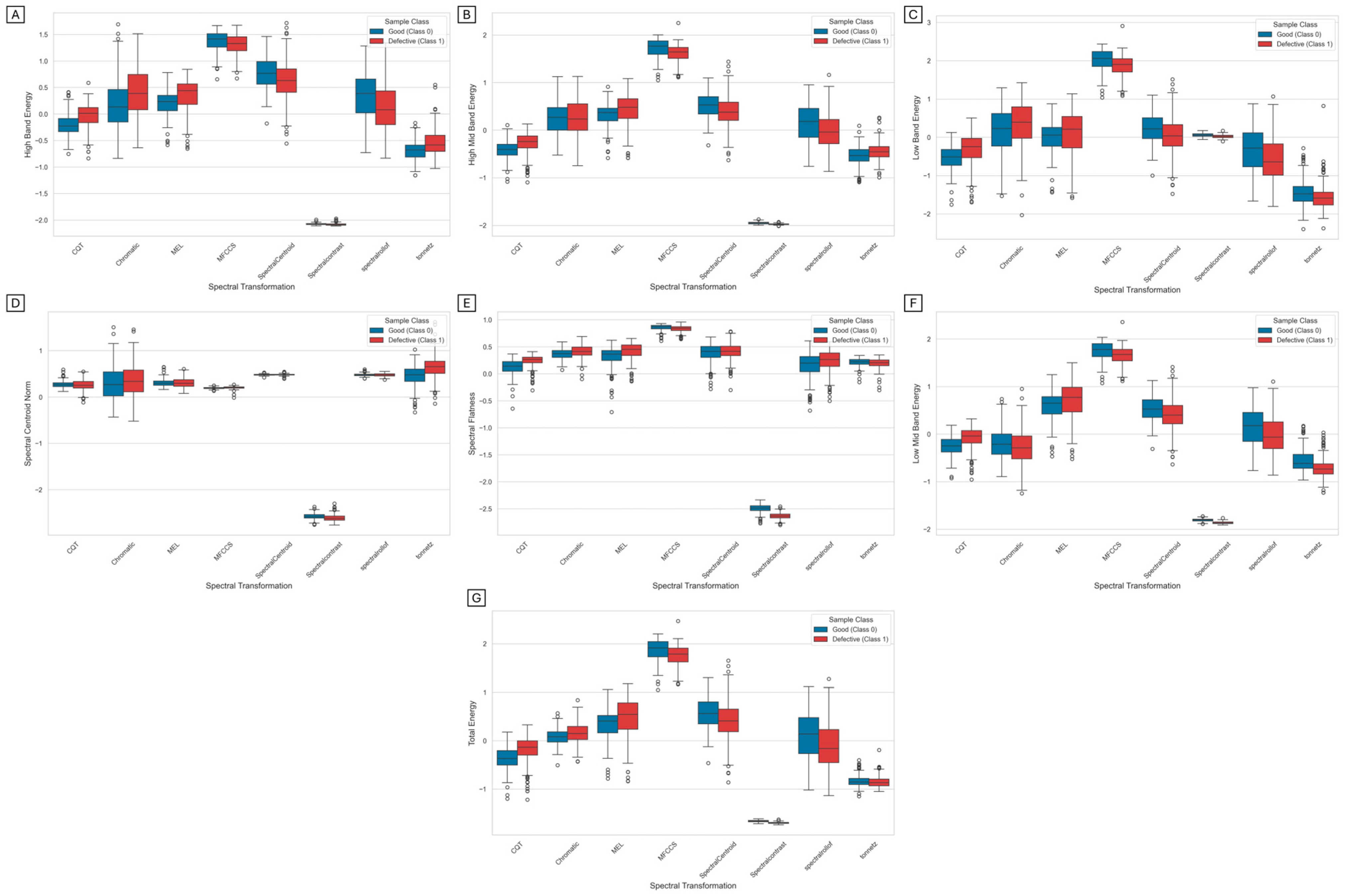
The boxplots in Figure 6 show the main spectral features extracted from different time–frequency transformations, differentiating between classes (0–1). Regarding metrics associated with spectral energy, a consistent pattern is observed across transformations. The MFCC and CQT transformations exhibit high median values, with medians at around 1.7–2.0 for MFCC and 1.8–2.1 for CQT in total energy, regardless of welding class. In contrast, transformations such as MEL and Chromatic display moderate energy values (0.4–0.8), with greater dispersion across their interquartile ranges, reflecting sensitivity to acoustic events associated with arc instabilities.

For the spectral centroid (D), the spectral rolloff transformation stands out by presenting the lowest values, with medians at around −1.8 and minimal dispersion. Similarly, for the spectral rolloff centroid (D), the transformation exhibits medians of −2.5, with narrow interquartile ranges and reduced class overlap, demonstrating a clear differentiation between tonal and noisy spectra for both spectral variables.

Overall, the results indicate that the MFCC and CQT transformations amplify spectral energy without enhancing class separability, whereas features based on the spectral shape (spectral flatness and centroid) exhibit greater statistical stability and physical relevance for the classification of SMAW welding quality.

3.3. Performance of Classification Models According to Spectral Transformation

Table 3. Performance of transformations according to the evaluated metrics.

Item	Transform	Accuracy	F1 Macro	Precision Macro	Recall Macro	ROC_AUC
a	Spectral contrast	0.901 ± 0.06	0.900 ± 0.06	0.909 ± 0.06	0.901 ± 0.06	0.955 ± 0.04
b	MEL	0.884 ± 0.09	0.882 ± 0.09	0.892 ± 0.09	0.884 ± 0.09	0.950 ± 0.05
c	CQT	0.883 ± 0.08	0.882 ± 0.08	0.887 ± 0.08	0.883 ± 0.08	0.949 ± 0.06
d	MFCC	0.847 ± 0.13	0.836 ± 0.15	0.860 ± 0.13	0.846 ± 0.13	0.921 ± 0.10
e	Cromatic	0.838 ± 0.07	0.837 ± 0.07	0.848 ± 0.07	0.839 ± 0.07	0.904 ± 0.06
f	Tonnetz	0.787 ± 0.09	0.785 ± 0.09	0.792 ± 0.09	0.787 ± 0.09	0.865 ± 0.08
g	Spectral centroid	0.781 ± 0.08	0.778 ± 0.08	0.794 ± 0.08	0.781 ± 0.08	0.857 ± 0.08
h	Spectral rollof	0.718 ± 0.09	0.714 ± 0.09	0.731 ± 0.10	0.719 ± 0.09	0.774 ± 0.09

presents the mean values and standard deviations of each metric for the different transformations evaluated, enabling a quantitative comparison of average performance and its stability. It is observed that the first three transformations (a–c) achieve the highest mean values, with classification metrics exceeding 0.88 and ROC-AUC values above 0.95, accompanied by low standard deviations (≈0.04–0.09), indicating consistent behaviour across patterns.

In contrast, transformations (d–h) exhibit lower means, particularly for Accuracy and F1-score (≈0.71–0.79). MFCC, on the other hand, shows competitive values compared to the other transformations; however, its high standard deviation (±0.15) indicates substantial variability in performance.

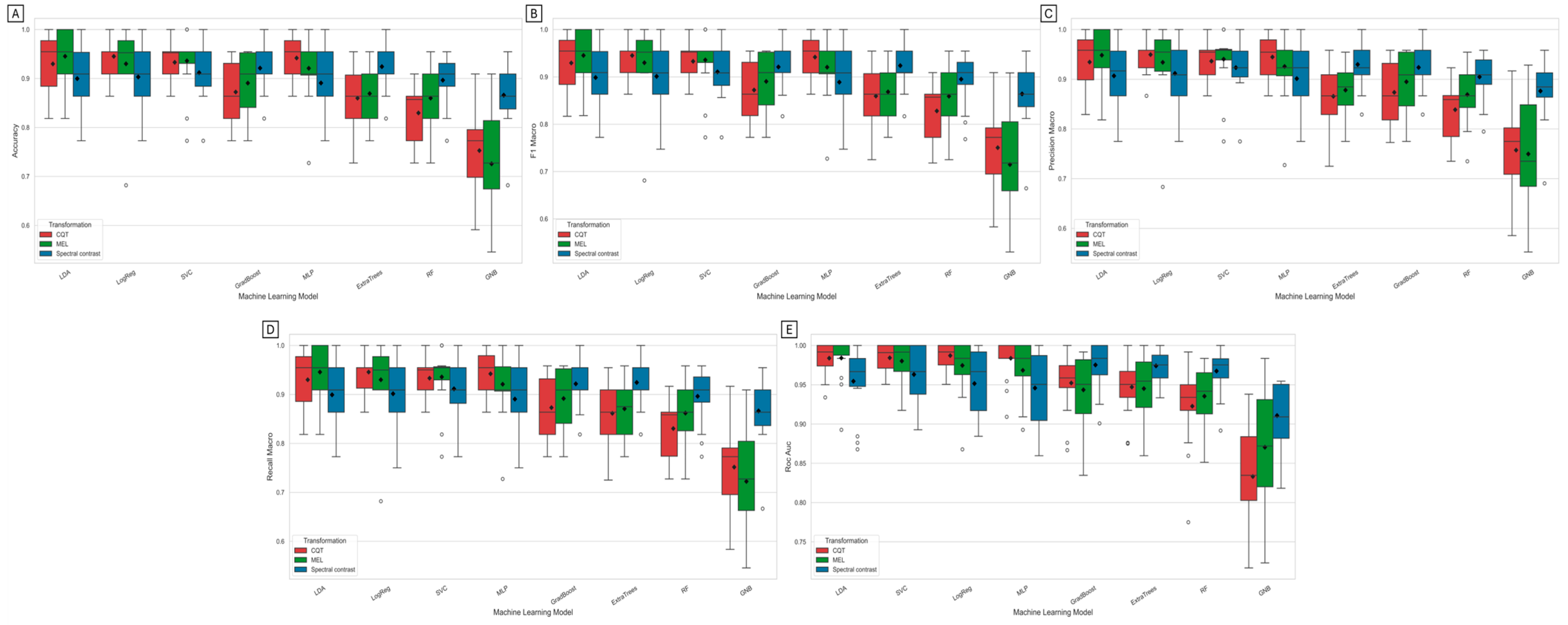
Figure 7 presents boxplots of the main evaluation metrics obtained for the different machine learning models under the primary transformations (CQT, MEL, and Spectral Contrast). Overall, the SVC, LDA, Logistic Regression, and MLP models demonstrate high and consistent performance, with ROC-AUC medians exceeding 0.95 for the three transformations, indicating a strong discriminative ability between welding classes. However, Spectral Contrast exhibits reduced interquartile dispersion, particularly in Gradient Boosting and Extra Trees models, reflecting greater model stability against data variations.

Macro F1 and macro recall metrics (Figure 7B,D), linear models and MLP maintain median values around 0.90–0.95 for Spectral Contrast and MEL, whereas CQT tends to show a slight decrease in ensemble-based models such as Random Forest and Extra Trees. This behaviour suggests that, although CQT is effective overall, it is sensitive to imbalances or intraclass variations. A similar trend is observed for macro precision, where Spectral Contrast achieves high medians (>0.90) and compact ranges, while GNB shows lower and less stable performance across all transformations (medians < 0.90).

3.4. Comparative Results of Top Models by Transformation

To identify the classifiers that maximise the predictive potential of the transformations, an analysis was conducted on the performance of the best-performing machine learning models for the transformations with the greatest impact on prediction.

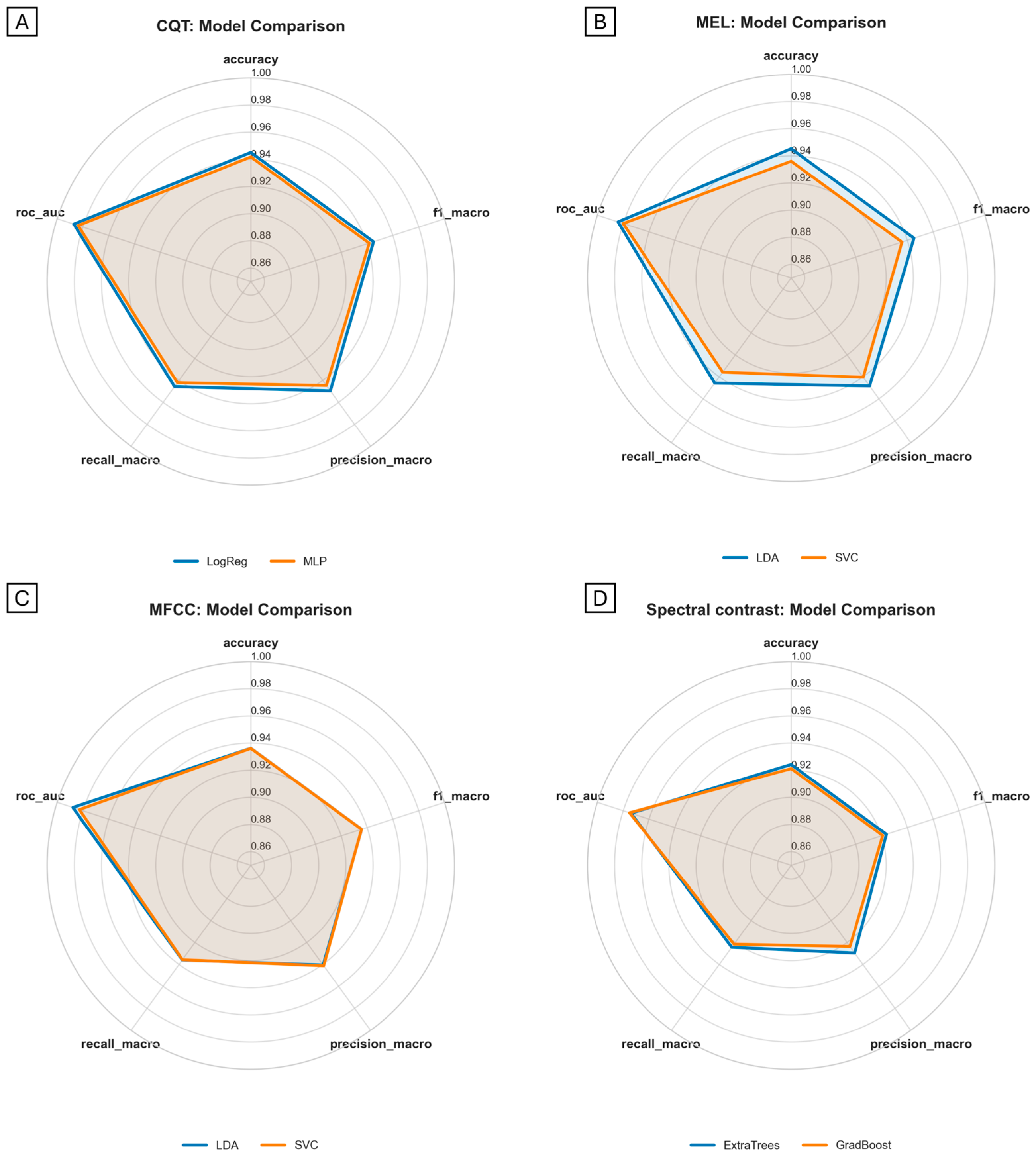
As shown in Figure 8, for Spectral Contrast, the Extra Trees and Gradient Boosting models achieved competitive performance, with Accuracy values above 0.92 and ROC-AUC values exceeding 0.97. For MEL, the LDA and SVC classifiers yielded the best results, with macro precision values above 0.93 and ROC-AUC values exceeding 0.98. Similarly, CQT demonstrated notable performance with Logistic Regression and MLP, achieving macro precision values of around 0.95. In the case of MFCC, LDA and SVC maintained stable behaviour, with Accuracy values exceeding 0.92.

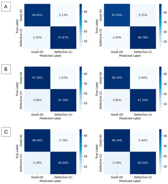
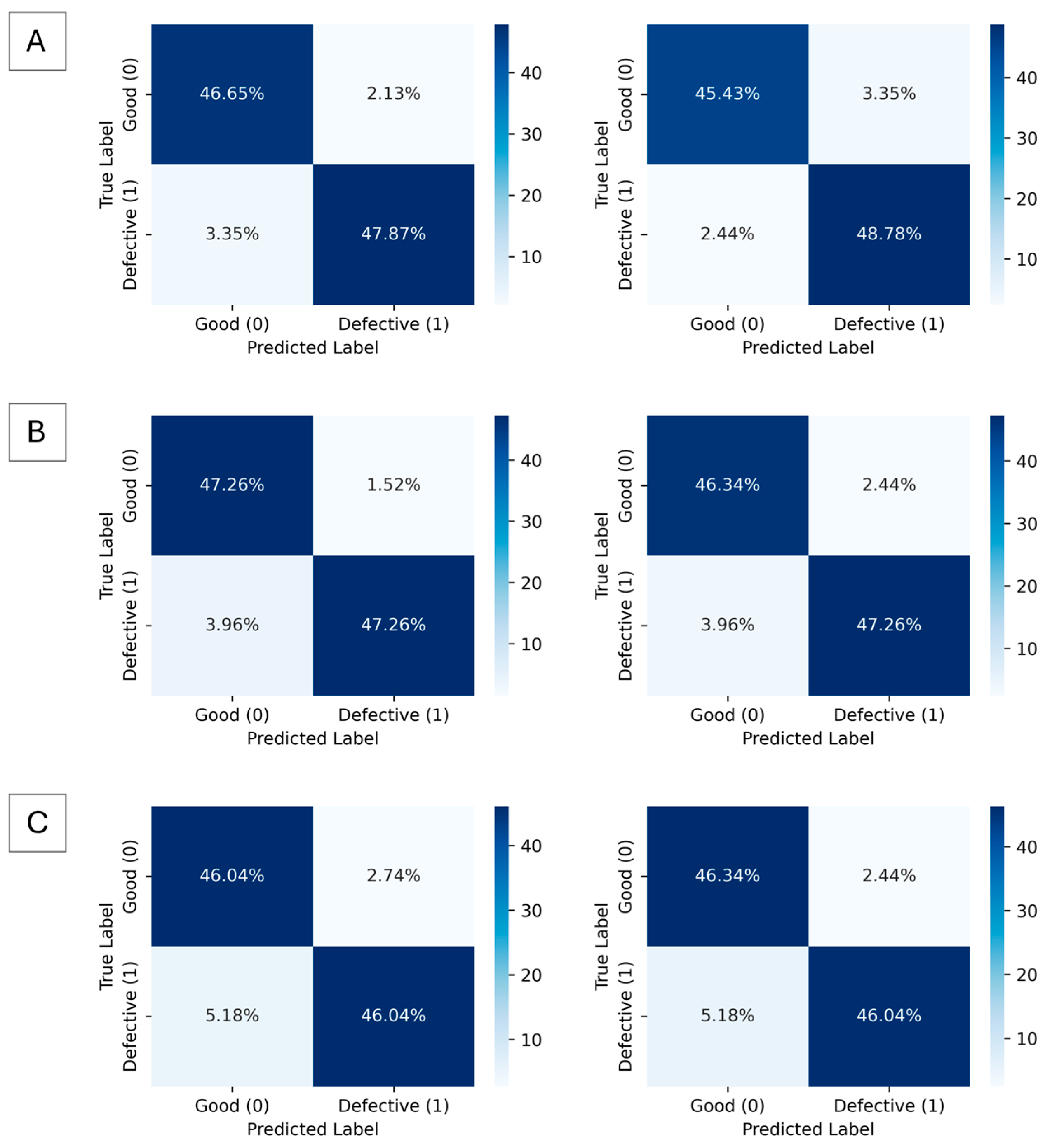
As a complement to the previous analysis, confusion matrices were examined for the three best-performing spectral transformations and their corresponding models, based on the results presented in Figure 8. This analysis aims to explicitly characterise the distribution of true and false classifications during the acoustic inspection of the SMAW process.

As shown in Figure 9, for the CQT transformation (A), both the Logistic Regression (LogReg) and MLP models achieved a correct identification of defective weld beads, with true positive (TP) values exceeding 50 samples in both cases, and false positives (FP) of 15 and 17 samples, respectively, in the classification of good welds. A reduction in false negatives (FN) is also observed, with fewer than 10 samples for both models. For the MEL transformation, the LDA model exhibited a balanced classification performance, with TN = 65 and TP = 55, and minimal cross-classification errors (FP and FN < 6). In contrast, the SVC model achieved a higher number of true positives (TP = 58), at the expense of an increased number of false positives, which is consistent with the reduction in its evaluation metrics observed in Figure 8.

For the Spectral Contrast transformation, the Extra Trees and Gradient Boosting models were consistent with the results shown in Figure 8, achieving stable and reliable confusion matrices, with more than 90% of the samples correctly classified. This performance is reflected in the reduction of false negatives (Gradient Boosting: FN = 3; Extra Trees: FN = 6), confirming the robustness of this spectral transformation for the acoustic characterisation of weld bead quality in the SMAW process.

In order to further evaluate the robustness of the evaluated classifiers, the variability of the performance metrics across the cross-validation folds was analyzed. For this purpose, the standard deviation of the obtained metrics was calculated together with the maximum and minimum values observed during the validation process. This analysis allows for assessing the stability of the models under different data partitions and verifying that the reported performance is not dependent on a specific train–test split. The results of this analysis are summarized in

Table 4. Variability of classification performance across cross-validation folds.

Transform	Model	Accuracy	f1_Macro	ROC_AUC	Max	Min
CQT	LogReg	0.039	0.039	0.015	1	0.863
	MLP	0.044	0.044	0.027	1	0.863
MEL	LDA	0.055	0.055	0.030	1	0.811
	SVC	0.064	0.064	0.026	1	0.772
Spectral Centroid	Extratrees	0.080	0.081	0.060	0.967	0.636
	Grad-Boost	0.063	0.063	0.050	0.967	0.725

.

The obtained deviations indicate moderate variability between folds, suggesting that the evaluated classifiers present consistent behavior across different partitions of the dataset.

In addition to classification performance, the computational cost of the evaluated models was analyzed to assess their potential suitability for real-time monitoring applications. Specifically, the training time and execution time of the best-performing transformation–model combinations were measured. The results, summarized in

Table 5. Computational cost of the best-performing transformation–model combinations.

Transform	Model	Fit_Time_Sec	Exec_Time_Sec
CQT	LogReg	0.072	15.019
	MLP	4.621	48.443
MEL	LDA	0.362	8.760
	SVC	0.029	2.674
Spectral Contrast	Extra Trees	2.146	25.160
	Grad Boost	14.348	479.971

, show notable differences in computational requirements between models. For instance, the SVC model combined with the MEL transformation presents the lowest execution time, whereas more complex ensemble models such as Gradient Boosting require significantly longer execution times. These results highlight the trade-off between classification performance and computational efficiency, which is a relevant factor when considering real-time acoustic monitoring systems for welding processes.

4. Discussion

4.1. Physical Interpretation of Acoustic-Based Classification Results

The results show that certain spectral transformations capture not only the total energy of the signal but also how this energy is distributed across spectral peaks and valleys, which is closely related to the physical dynamics of the SMAW process. In this process, arc stability and the regularity of metal transfer generate acoustic patterns with a defined spectral structure, whereas instabilities manifest as abrupt variations in the spectrum.

The Spectral Contrast transform emphasises local differences between peaks and valleys in the spectrum, allowing for improved discrimination of acoustic irregularities caused by bead defects compared to a stable arc. This transformation has been highlighted in acoustic classification studies in audio tasks where capturing the relative energy distribution across sub-bands provides better discrimination between sound classes that share similar spectral patterns but differ in local matrices [23]. Transformations such as MEL and CQT are also widely used spectral representations in acoustic signal classification; however, the variability observed in this study suggests that they are not always sufficient to highlight local details relevant to defects in SMAW acoustic signals.

The observation that ensemble-based ML models (Gradient Boosting and Extra Trees) achieve the highest combined precision scores with Spectral Contrast (>0.92) can be related to the way these algorithms handle complex nonlinear relationships between features (spectral peaks and valleys). This aligns with previous acoustic classification studies demonstrating that combinations of detailed spectral features and nonlinear models can improve classification accuracy and stability compared to simple linear methods [14]. Conversely, the poor performance of the Gaussian Naïve Bayes model indicates that feature independence assumptions do not hold for complex acoustic signals such as those from a welding arc, where inherent correlations exist between spectral components and physical process events.

4.2. Comparison with Related Acoustic-Based Welding Quality Studies

To contextualise the obtained results,

Table 6. Comparison between acoustic welding studies and the present work.

Author/ Study	Type of Welding	Characteristics	Model ML	Metrics
Jang et al. (2024) [24]	GTAW pulsado	Sound of arc + FFT + EEMD	Machine Learning	F1 score > 0.91
Ji & Norzalilah (2023) [14]	SMAW (digital twin acústico)	Acoustic signal, time-frequency representations	Hybrid CNN (SeCNN-LSTM)	Accuracy ≈ 0.91
Zhang et al. (2024) [25]	DED-Arc	Wavelet time-frequency	CNN (ResNet, MobileNetV3)	Accuracy 0.96–0.98
Actual Project	SMAW	Spectral contrast, MEL CQT	Extra Trees, GBoost, SVC, LDA	Accuracy ≈ 0.90–0.92; ROC AUC > 0.95

presents a comparison between this study and previous works that addressed defect detection and classification in welding processes using acoustic signals, spectral descriptors, and machine learning. The comparison is made using metrics commonly reported in the literature to evaluate the performance of acoustic and welding monitoring systems (precision, recall, F1-score, and accuracy). Although differences exist in experimental configurations and algorithms employed, the studies consistently indicate that the spectral features of the acoustic signal contain relevant information regarding arc stability and the presence of defects in the welding bead.

In comparison with other recent studies, the metric results of this work demonstrate equivalent performance using a more practical approach. While previous research reports accuracy and F1-score values in the range of 0.90–0.96 using neural networks and acoustic signals in different types of controlled and non-human-operated welds, this study achieves accuracies above 0.90 and ROC-AUC values exceeding 0.95 in SMAW welding using classical spectral transformations. This indicates that, unlike approaches based on complex models, the characterisation of the spectral contrast of the arc sound effectively captures the physical instabilities associated with defects in SMAW welding beads.

5. Future Works

Due to the limited size of the available dataset, the evaluation relied on stratified ten-fold cross-validation rather than a fixed hold-out test set. This approach ensures that all samples contribute to both training and validation while maintaining class balance across folds. Although this strategy provides a robust estimate of model performance, future work will focus on validating the proposed approach using larger datasets and independent test sets collected under different welding conditions.

6. Conclusions

This study evaluated the effectiveness of several spectral and time–frequency representations derived from acoustic signals for the automated classification of weld bead quality in manual SMAW welding processes. Rather than introducing a new methodological framework, the objective of the work was to systematically compare how different spectral transformations influence classification performance in the context of acoustic-based weld quality monitoring.

Among the evaluated representations, spectral contrast consistently provided the most discriminative information, enabling ensemble models such as Extra Trees and Gradient Boosting to achieve robust and well-balanced performance across the evaluated metrics. These results highlight the importance of selecting appropriate signal representations when designing acoustic monitoring systems for welding processes.

The analysis of the confusion matrices confirmed a reliable separation between weld quality classes, characterised by low misclassification rates and stable responses for both true positive and true negative detections. Although individual spectral descriptors show considerable overlap in the exploratory analysis, their combined use within machine learning models allows the capture of acoustic patterns associated with arc instability and welding defects.

The results demonstrate that classical spectral representations, when combined with well-established machine learning algorithms, provide an effective and computationally efficient approach for acoustic monitoring of manual welding operations. These findings contribute to the development of practical and low-cost monitoring systems capable of assisting weld quality assessment in industrial environments.

References

- Jan, Z.; Ahamed, F.; Mayer, W.; Patel, N.; Grossmann, G.; Stumptner, M.; Kuusk, A. Artificial intelligence for Industry 4.0: Systematic review of applications, challenges, and opportunities. Expert Syst. Appl. 2023, 216, 119456. [Google Scholar] [CrossRef] [Scilit]
- Ördek, B.; Borgianni, Y.; Coatanea, E. Machine learning-supported manufacturing: A review and directions for future research. Prod. Manuf. Res. 2024, 12, 2326526. [Google Scholar] [CrossRef] [Scilit]
- Rahman, M.A.; Shahrior, M.F.; Iqbal, K.; Abushaiba, A.A. Enabling Intelligent Industrial Automation: A Review of Machine Learning Applications with Digital Twin and Edge AI Integration. Automation 2025, 6, 37. [Google Scholar] [CrossRef] [Scilit]
- Kausik, A.K.; Rashid, A.B.; Baki, R.F.; Maktum, M.M.J. Machine learning algorithms for manufacturing quality assurance: A systematic review of performance metrics and applications. Array 2025, 26, 100393. [Google Scholar] [CrossRef] [Scilit]
- Benhanifia, A. Systematic review of predictive maintenance practices in manufacturing sector. Intell. Syst. Appl. 2025, 26, 200501. [Google Scholar] [CrossRef] [Scilit]
- Ani, O. Advanced Manufacturing with Machine Learning: Improving Predictive Maintenance, Quality Control, and Process Optimization. Rafidain J. Eng. Sci. 2024, 2, 280–300. [Google Scholar] [CrossRef] [Scilit]
- Delzendehrooy, F.; Akhavan-Safar, A.; Barbosa, A.; Beygi, R.; Cardoso, D.; Carbas, R.; Marques, E.; da Silva, L. A Comprehensive Review on Structural Joining Techniques in the Marine Industry; Elsevier: Amsterdam, The Netherlands, 2022. [Google Scholar] [CrossRef] [Scilit]
- Nelson, J.P.; Biddle, J.B.; Shapira, P. Applications and Societal Implications of Artificial Intelligence in Manufacturing: A Systematic Review. arXiv 2023, arXiv:2308.02025. [Google Scholar] [CrossRef] [Scilit]
- Zhou, J.; Mohammad, A.; Zeng, T.; Axinte, D.; Wright, I.; March, R. Teaching robots to weld by leveraging human expertise. Robot. Comput. Manuf. 2025, 95, 103027. [Google Scholar] [CrossRef] [Scilit]
- Kim, I.S.; Son, J.S.; Yang, Y.S.; Yaragada, P.K.D.V. Sensitivity analysis for process parameters in GMA welding processes using a factorial design method. Int. J. Mach. Tools Manuf. 2003, 43, 763–769. [Google Scholar] [CrossRef] [Scilit]
- Jin, C.; Rhee, S. Real-Time Weld Gap Monitoring and Quality Control Algorithm during Weaving Flux-Cored Arc Welding Using Deep Learning. Metals 2021, 11, 1135. [Google Scholar] [CrossRef] [Scilit]
- Liu, Y.K.; Zhang, W.J.; Zhang, Y.M. A tutorial on learning human welder’s behavior: Sensing, modeling, and control. J. Manuf. Process. 2014, 16, 123–136. [Google Scholar] [CrossRef] [Scilit]
- Fahle, S.; Prinz, C.; Kuhlenkötter, B. Systematic review on machine learning (ML) methods for manufacturing processes—Identifying artificial intelligence (AI) methods for field application. In Procedia CIRP; Elsevier: Amsterdam, The Netherlands, 2020; pp. 413–418. [Google Scholar] [CrossRef] [Scilit]
- Nor, M. Deep Learning-Empowered Digital Twin Using Acoustic Signal for Welding Quality Inspection. Sensors 2023, 23, 2643. [Google Scholar] [CrossRef] [Scilit] [PubMed]
- Sumesh, A.; Ramesh Kumar, K.; Mohandas, K.; Babu, R.S. Use of Machine Learning Algorithms for Weld Quality Monitoring using Acoustic Signature. Procedia Comput. Sci. 2015, 50, 316–322. [Google Scholar] [CrossRef] [Scilit]
- Koal, M.; Povel, C.; Furrer, J.; Wohlhaupter, M. Acoustic process monitoring during projection welding using airborne sound analysis and machine learning. Weld. World 2025, 69, 459–470. [Google Scholar] [CrossRef] [Scilit]
- Schmidt, L.; Römer, F.; Böttger, D.; Leinenbach, F.; Straß, B.; Wolter, B.; Schricker, K.; Seibold, M.; Bergmann, J.P.; Del Galdo, G. Acoustic process monitoring in laser beam welding. Procedia CIRP 2020, 94, 763–768. [Google Scholar] [CrossRef] [Scilit]
- Luo, Z.; Wu, D.; Zhang, P.; Ye, X.; Shi, H.; Cai, X.; Tian, Y. Laser welding penetration monitoring based on time-frequency characterization of acoustic emission and CNN-LSTM hybrid network. Materials 2023, 16, 1614. [Google Scholar] [CrossRef] [Scilit] [PubMed]
- National Instruments. Parseval’s Theorem. Available online: https://www.ni.com/docs/en-US/bundle/labwindows-cvi/page/advancedanalysisconcepts/lvac_parseval_s_theorem.html (accessed on 16 January 2026).
- Spectral Centroid—Engineering Definition. ScienceDirect Topics. Available online: https://www.sciencedirect.com/topics/engineering/spectral-centroid (accessed on 22 January 2026).
- Dwivedi, D.; Haragopal, V.V. Contrast between simple and complex classification algorithms. In Statistical Modeling in Machine Learning; Concepts and Applications; Dwivedi, D., Haragopal, V.V., Eds.; Elsevier: Amsterdam, The Netherlands, 2023; pp. 93–110. [Google Scholar] [CrossRef] [Scilit]
- Dubnov, S. Generalization of Spectral Flatness Measure for Non-Gaussian Linear Processes. IEEE Signal Process. Lett. 2004, 11, 698–701. Available online: https://ieeexplore.ieee.org/document/1316889 (accessed on 28 January 2026). [CrossRef] [Scilit]
- Gupta, S.; Srivastava, V.; Kumar, D. Environment Sound Classification Using Stacked Features and Convolutional Neural Network. In Proceedings of the 2024 Sixteenth International Conference on Contemporary Computing (IC3 2024), Noida, India, 8–10 August 2024. [Google Scholar] [CrossRef] [Scilit]
- Jang, S.; Lee, W.; Jeong, Y.; Wang, Y.; Won, C.; Lee, J.; Yoon, J. Machine Learning-Based Weld Porosity Detection Using Frequency Analysis of Arc Sound in the Pulsed Gas Tungsten Arc Welding Process. J. Adv. Join. Process. 2024, 10, 100231. [Google Scholar] [CrossRef] [Scilit]
- Zhang, H.; Wu, Q.; Tang, W.; Yang, J. Acoustic Signal-Based Defect Identification for Directed Energy Deposition-Arc Using Wavelet Time–Frequency Diagrams. Sensors 2024, 24, 4397. [Google Scholar] [CrossRef] [Scilit] [PubMed]
Disclaimer/Publisher’s Note: The statements, opinions and data contained in all publications are solely those of the individual author(s) and contributor(s) and not of MDPI and/or the editor(s). MDPI and/or the editor(s) disclaim responsibility for any injury to people or property resulting from any ideas, methods, instructions or products referred to in the content. |
© 2026 by the authors. Licensee MDPI, Basel, Switzerland. This article is an open access article distributed under the terms and conditions of the Creative Commons Attribution (CC BY) license.