Use of Machine Learning for Solar Power Generation Prediction in the Field of Alternative Renewable Energy Sources

Abstract

This study focused on the application of supervised learning in the field of renewable energy, specifically for predicting daily solar irradiance in Neiva, department of Huila, Colombia. To this end, decision tree and artificial neural network (DT and ANN, respectively) models were trained and tested using the online tool Google Colab. The main objective was based on the need to optimize energy planning processes at local and regional levels, motivated by the increase in demand for the integration of non-conventional energy sources and the spatial–temporal variability in solar resources in the country. A dataset consisting of 366 daily records for the year 2024 was obtained from the NASA POWER database at the geographic coordinates (2.930079, −75.255650) and used for training and evaluating the proposed models. Statistical and cleaning techniques were used, including the treatment of outliers using the moving-window median for the latter. Metrics, such as mean absolute error ($MAE$), root mean square error ($RMSE$), and coefficient of determination ($R^2$), were used to evaluate the models. Data inclusion and exclusion criteria were applied to ensure the quality and validity of the observations. Model performance was evaluated using a randomized Hold-Out validation strategy (90% training and 10% testing), which was repeated across multiple iterations. The performance metrics reported corresponded to the 10th iteration of the validation process after outlier treatment. Under this configuration, the DT model achieved a higher predictive performance ($R^2$ = 0.8882) compared with the ANN model ($R^2$ = 0.7679), demonstrating its effectiveness as a reliable approach for estimating daily solar irradiance under the studied conditions. This result was also confirmed by the decreased $MAE$ and $RMSE$ for the DT model, which indicated that this model performed better in predicting the real values than the ANN model. Finally, the added value of the study is to consolidate national evidence and open access tools to facilitate the development of sustainable energy policies in intermediate cities such as Neiva.

1. Introduction

Low-carbon and clean energy technologies for sustainable electricity generation can play a significant role in curbing climate change and contributing to the global energy transition [1]. Many nations around the world are also seeking to diversify their energy mix with cleaner, environmentally sustainable, and cost-effective sources of energy [1,2,3]. National commitments to reduce greenhouse gas (GHG) emissions by 51% by 2050 (in accordance with the Nationally Determined Contribution (NDC)) are established in Colombia under the Paris Agreement [1,2,3]. This goal hinges upon multifaceted mitigation strategies, such as the decarbonization of the energy system, the implementation of low-carbon technologies, and the strengthening of energy efficiency policies to achieve climate neutrality in the expected time frame [4,5,6].

Nowadays, the power generation sector has historically been one of the largest contributors to global GHG emissions. Electricity generation was responsible for about 29% of total GHG emissions in 2015, followed by the transportation sector (27%) and industrial production (21%) [7]. In Colombia, the energy sector accounts for nearly one-third of the country’s net GHG emissions and is a focal point in national decarbonization efforts [3]. In order to respond to these challenges, the United Nations established the 2030 Agenda for Sustainable Development in 2015, which constitutes a global roadmap for sustainable development. However, the National Planning Department (DNP, in Spanish) points to the current obstacles to progress toward the Sustainable Development Goals (SDGs) in Colombia as being the persistent social inequality, the structural policy limitations, the legacy of armed conflict, and the economic impacts of COVID-19. The challenges mentioned above show that more policy coordination and technological innovation are needed in the energy sector to make a difference [8,9].

Solar radiation is a renewable energy resource which is naturally occurring and abundant. This resource is crucial for photosynthesis and other vital functions for life and ecology on Earth [10,11,12]. From an energy perspective, solar radiation is an electromagnetic wave that sends off the energy generated when sunlight hits a target location in space. According to Trenberth [13], the average solar irradiance received by Earth is about 1.368 kW/m². Irradiance, on the other hand, quantifies the energy received over an interval of time and is expressed in kWh/m² [14]. This parameter represents an important criterion for assessing the solar energy potential, as well as for designing photovoltaic (PV) systems and planning solar energy projects [15,16]. In the Colombian context, Eras et al. [17] estimated the daily average solar radiation to be about 4.5 kWh/m²/day, compared to high-potential areas, like La Guajira, where the values were likely to reach 6.0 kWh/m²/day, depending on local geographical and climatic conditions.

Solar resources can be delivered in a local form via PV modules or solar cells, which have a reduced environmental impact. Meanwhile, thermal energy can also be provided by solar radiation largely in cases such as in fluid heating techniques for solar collectors and in water treatment processes [18]. Solar energy is a lower carbon energy form and, with respect to fossil fuels, reduces GHG emissions [19]. Nevertheless, the effective application of solar energy systems is uncertain because of conversion efficiencies, resource intermittency, and localized climatic conditions. In addition, the spatial and temporal variability in solar radiation, combined with limited high-resolution meteorological information, continues to pose challenges for accurate PV application, modeling and optimization [20].

Despite the rapid development of renewable energy technologies which have been established to be fundamental to climate change mitigation, there are still significant issues regarding energy security, affordability, and cost-effectiveness [21]. In this context, artificial intelligence (AI), especially machine learning (ML), has become crucial for the analysis and management of renewable energy systems such as solar, wind, hydroelectric, and wave energy [22]. In solar PV systems, predictive models can include fundamental meteorological and environmental parameters like global horizontal irradiance, ambient temperature, cloud cover indices, wind speed and direction, ultraviolet radiation, relative humidity, and atmospheric pressure. The accurate characterization of these variables through ML methods can improve solar forecasting, facilitate the planning of PV projects, and enhance the integration of renewable energy into modern power systems [23,24].

Computational modeling and numerical methods have emerged as important approaches for the analysis and optimization of modern energy systems, especially those related to alternative renewable energies through development and management processes. Such methods support the examination of complicated physical processes and aid in more effective application of energy resources. In recent years, various studies have found that advanced modeling techniques are extremely useful in energy applications (e.g., geothermal and emerging energy resources) [25,26]. ML techniques are now of increasing importance within this domain as data-driven methods for capturing non-linear relationships in large-scale datasets that can be employed in renewable energy applications. For instance, up-to-date ML models have gained traction in the field of solar energy systems used to predict solar irradiance and power production, and yield useful information in the planning, management and optimization of PV energy generation [27,28,29].

Supervised learning remains the most preferred paradigmatic approach in the field of ML for training models in the process of transforming independent variables (input features) into dependent variables (output labels) to extract informative functions from the data that capture underlying patterns [30]. The mechanism allows for optimizing loss functions to reduce the likelihood of making prediction errors [31,32], allowing this learning to be executed for classification and regression. Furthermore, for synthetically making predictions via data augmentation or for developing a ML model to enhance its capabilities in these data-limited or sparse scenarios [32], supervised learning methods can be utilized in the developing generative models.

Several techniques are commonly used to represent complex non-linear relationships in energy systems, particularly in the form of artificial neural network (ANN) or decision tree (DT) models. DT models have also been applied to evaluate the likelihood and effectiveness of renewable energy policies [33]. These models can incorporate well-structured input data, such as geographic variables [34], regulatory and policy factors [35], and other socio-technical parameters. By incorporating these variables into algorithms, context-specific dependencies can be captured, performing scenario analyses and providing useful insights for energy planning and policy evaluation.

Under this framework, the present study aims to evaluate the performance of two ML models based on DT and ANN techniques to predict solar irradiance as the response variable using daily data reported for 2024. The NASA POWER (NP) database was used as the primary source for obtaining training and testing data. In addition, the Google Colab platform was employed as the computational environment due to its accessibility and compatibility with Python-based programming tools. Model performance was evaluated using several statistical metrics commonly reported in the literature, as described in the following sections.

2. Materials and Methods

2.1. Background

Studies, such as those conducted by Z. Allal et al. [36] and Ajibade et al. [37], used supervised learning in the renewable energy sector. For solar energy, ML algorithms were used even for multiple linear regressions [38,39], DT [40,41,42,43] and ANN [44,45,46,47]. Currently, great advances have been reported in the use of open datasets for solar prediction. In this regard, the research carried out by N. Singh [41] and collaborators analyzed the accuracy of three models: (i) Logistic Regression, (ii) Random Forest (RF) and (iii) the DT model. The referenced authors trained the three models and used an exploratory analysis of the data to determine the correlation and dispersion between them, concluding that the DT model demonstrated an accuracy of 98% in the prediction of solar irradiance (output variable) compared to 51% and 55% for the first and second models, respectively. In turn, J. Sánchez et al. [48] used real data from a solar farm located in Canada, which was divided into four zones. The authors used the DT model because of its low computational cost and great effectiveness in training and testing, for which they used spatial and temporal correlation. The DT models the referenced authors analyzed were RF, Gradient Boosting Machine (LGBM) and Extreme Gradient Boosting (XGB). During the evaluation process, they used the mean absolute percentage error (MAPE) and the mean absolute error ($MAE$) metrics, finding that the LGBM method was slightly superior to the others. As a matter of fact, in the third zone, the MAPE for this model was 4.195 versus 4.394 and 4.358 observed for RF and XGB, respectively. On the other hand, $MAE$ was 27.848 versus 28.974 and 28.623 for RF and XGB, respectively. In turn, S. N. Shorabeh et al. [40] compared the optimization models based on the particle swarm optimization (PSO) algorithm and the DT model. The authors employed criteria maps, assigning weights to each criterion and generating the special maps, and then selected training samples for the two models. Shorabeh and co-researchers determined that the DT model had a high prediction potential versus PSO; thus the prediction rates for the DT and PSO were 0.29 and 0.13, respectively. In that sense, a better modeling capability of areas conducive for solar power project projection would be offered by employing the DT method. Rahul et al. [42], using the DT method, predicted the daily generated power output from 1 May 2015 for a period of 5 years at the solar farms in Gujarat Power Corporation Limited, India, and contrasted it with meteorological data derived from NP Project. The authors used 21.4% of the data for testing and the remaining (78.6%) for model training; additionally, they employed $MAE$, MAPE and mean square error (MSE) to compare the accuracy and reliability of the model.

In turn, Kassim et al. [43] employed an AI model based on the adaptive DT model to forecast the power output of a solar farm built in Malaysia with a capacity of 50 MW. The data used allowed for feeding of the Decision Tree Regressor (DTR) function of the Sklearn library and comprised the temporal range covering from June 2019 to December 2020. Subsequently, these data were exported in .csv format and downloaded in two fractions: (i) the first range was defined for training and covered from 1 June to 31 December 2019 and (ii) the second was defined for model testing and covered from 1 January to 31 December 2020. The authors employed $MAE$, the coefficient of determination ($R^2$) and Pearson’s correlation coefficient (r) to compare the model approximation against the three cases and two types of datasets for training and testing the model: (i) the first uses all data from five weather stations, (ii) the second uses the average data from the five weather stations and (iii) the third uses an index correlation of more than 0.8. The results showed that case 1 (i) had the highest $MAE$ and r, which did not represent a good approximation compared to the other cases. The authors did not determine which one of the three cases was the most appropriate, since, although case 3 (iii) had a lower $MAE$, a low $R^2$ was found. Therefore, the most relevant case for prediction was still unclear.

Essam et al. [49] studied several ML models aimed at estimating solar PV energy production, which were trained on data obtained from the U.S. National Renewable Energy Laboratory (NREL) for the city of Cocoa located in Brevard County, Florida. The authors compared ML models such as ANN, XGB, RF and long short-term memory (LSTM). ANN was found to have a high performance, adequately representing the output variable, even with a superior capability compared to the other algorithms. Similarly, the authors found that the DT method was highly recommended for predicting less volatile data, such as daily solar PV energy production, versus more volatile instantaneous data. For this reason, the present research is based on a daily, rather than instantaneous (i.e., hourly, minute or second), dataset.

Finally, Toylan et al. [44] utilized the DT algorithm to predict short-term solar irradiance to train the model. The authors used four input variables: (i) month, (ii) day, (iii) hour, and (iv) air temperature. Additionally, they considered solar irradiance as the output variable. The research used the $R^2$ and $RMSE$ metrics to compare the accuracy of the trained model, and the values obtained were 0.97 and 91.282, respectively.

Under this scenario, according to the reports found in the literature, it is observed that authors have focused their research on the comparative analysis of various AI models for predictive modeling of solar radiation time series, employing standardized statistical evaluation metrics (e.g., $MAE$, $RMSE$, and $R^2$). Nevertheless, a significant gap persists in the literature regarding the optimized implementation of supervised learning algorithms, particularly in multivariate regression and ensemble methods, adapted to the specific climatic and geographical conditions in the Colombian context, such as those found in Neiva, department of Huila.

2.2. Implementation and Training of Predictive Models

The predictive models were implemented in a supervised learning approach based on the preprocessed dataset that was split into training and testing sets to enhance the generalizability and prevent the risk of information leakage. The implementation concerning the DT model was carried out using the CART algorithm that can implement recursive binary feature space partitioning. The training process followed a greedy optimization strategy in which, at each node, the algorithm evaluated all input variables and possible split points to determine the optimal threshold that maximized variance reduction or, equivalently, minimized the MSE in the resulting child nodes. A recursive partitioning took place till predefined stopping constraints were met, such as maximum tree depth or minimum number of samples per leaf node. After that, a number of hyperparameters were evaluated in this stage to optimize the trade-off between the complexity of a model and the predictive performance. After model tuning, the final model had no maximum tree depth (no depth restriction), needed 2 samples for internal node split and had a minimum number of samples to find a leaf node of 1. These values were chosen to control model complexity, reduce variance, and avoid overfitting while allowing the model to take into account the stochastic variability and non-linear property of solar irradiance.

In contrast, the ANN model was created based on a feedforward multilayer perceptron architecture, consisting of an input layer, two hidden layers, and an output layer. The input layer received two predictor variables, namely the month and the day, which represented the temporal position of each observation within the annual cycle. In the hidden structure, 16 neurons were contained in the first hidden layer compared to 8 neurons in the second hidden layer. These layers modeled the non-linear relationships between the input variables and the target variable through non-linear activation functions, including ReLU, Sigmoid, and Tanh, which were evaluated during the training process. The output layer contained a single neuron with a linear activation function to estimate the predicted value of daily solar irradiance. The network was trained using the Adam optimization algorithm. Unlike the deterministic partitioning strategy of the DT model, ANN training is an iterative optimization by backpropagation. In every epoch when training, the input was forward propagated to output from the network to make a prediction for the input, and in this way it could be correlated with the observed values using a loss function. Once the output was generated, the resultant error was propagated back through the network backwards to obtain gradients for weights and biases in the model. An optimization algorithm would update the parameters in a similar manner to Adam or Stochastic Gradient Descent, as they updated in a form that minimized the loss function. This iterative process was repeated until convergence to a steady minimum, or until an early stopping criterion was enabled to prevent overfitting. This iterative nature of the optimization model contributed to the differences among various training schemes tested in our report. Thus, a systematic hyperparameter tuning phase to check whether the parameter distribution was suitable for both models was done in an iterative manner. For the DT model, the structure complexity was regulated by tree depth and minimum samples per node and for the ANN model, the number of hidden layers and neurons for each layer were tuned. Each configuration was numerically verified in a testing set of $R^2$ and error measures, including $MAE$ and $RMSE$.

2.3. Geographical Location

This research studies the city of Neiva, department of Huila, Colombia, which is characterized by a high global horizontal irradiance (GHI > 3.5 kWh/m²/day) and atypical cloud patterns. These traits make Neiva a suitable natural laboratory to verify solar energy prediction models with dry tropical environments, as well as to perform hyperparameter tuning of supervised learning algorithms. The city shows dry tropical weather that always rises above the national average. In Colombia, the average monthly maximum temperatures range from 24 to 28 °C and cover over 50% of the territory, placing Neiva (2.930079, −75.255650) at the upper end of this range (IDEAM, [50]). It is known from historical records that maximum temperatures have been recorded at 39.2 °C [51], with substantial demand for cooling systems in residential, commercial and industrial sectors. This demand has resulted in a sharp concentration in the electrical load curve during hours with maximum solar insolation (10:00–15:00 h).

The accelerated deployment of grid-connected PV systems was conducted in Neiva during 2018–2023 and optimized for tilt angles between 15° [52] and 16° [53] based on spectral irradiance studies for flat surfaces. This setup gave the optimal absorption of the direct normal irradiance at a high-insolation stage, with its annual mean solar energy being >2500 kWh/m²/year (>4.65 kWh/m²/day), which is a typical climatic characteristic for this region. Policies, such as Law 1715 of 2014 [54], whose regulations are followed [55], offer financial incentives, including 50% income tax deductions and accelerated depreciation schemes to allow such systems to be deployed for renewable energy projects to extend PV systems. These measures, along with 30–40% levelized PV energy cost reduction, have made Neiva a prime example of solar electricity generation in Huila and the integration of climatic, technological and policy forces acting as catalysts for sustainable energy installation.

2.4. Sample

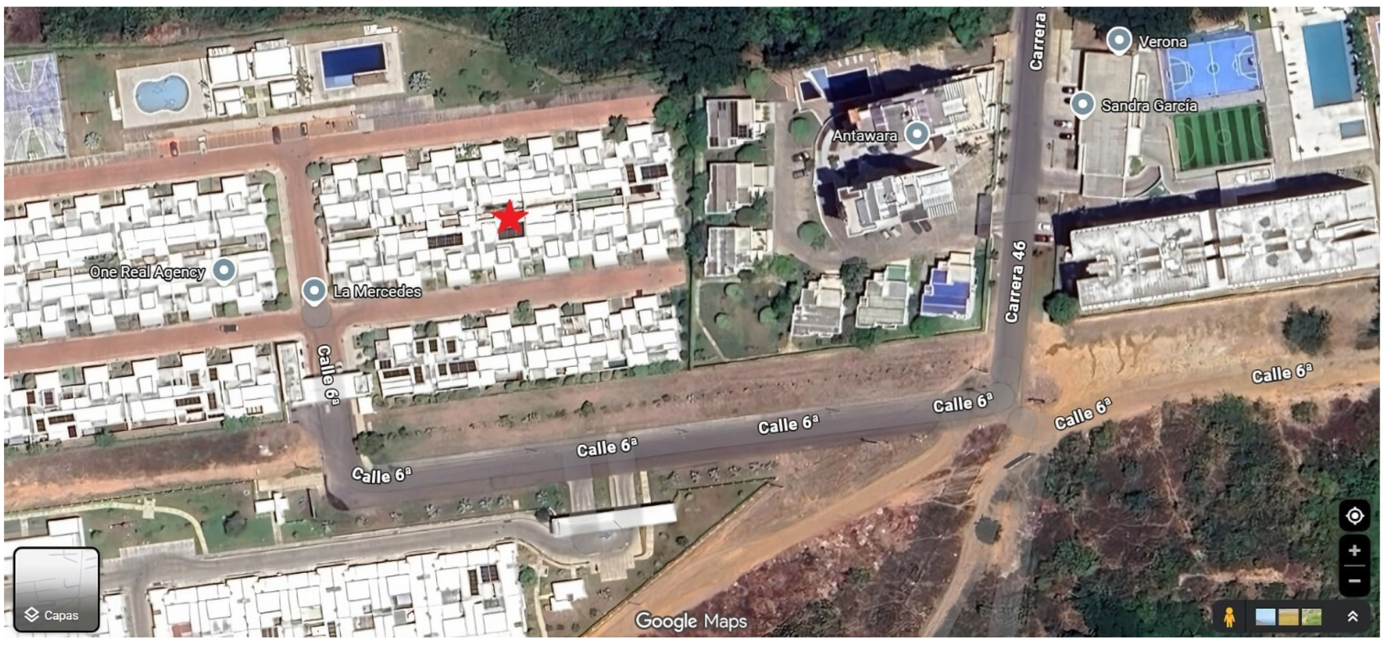
At the georeferenced site stated above, this sample involved solar irradiance measurements. The site chosen for the study (2.930079, −75.255650), as shown in Figure 1, was selected based on spatially optimized considerations, along with the high exposure to global horizontal irradiance (GHI > 4.65 kWh/m²/day), the low topographic shading, and over 95% free horizon for the east–west sector. These factors, therefore, enable maximum solar resource availability in addition to reliability of irradiance data to be ensured for the calibration and validation of the predictive PV models.

Figure 1. Coordinates 2.930079, −75.255650. Source: Google Maps. Geographical location of the reference point (red star) located in Neiva, department of Huila, Colombia.

The dataset contained 366 observations, corresponding to the daily average solar irradiance values (in kWh/m²/day) recorded during the year 2024, which was a leap year. Each observation represented the solar irradiance associated with a specific day of the annual cycle.

The use of a single calendar year was consistent with the structure of the predictive model implemented in this study. Solar irradiance was modeled using two temporal explanatory variables, namely the month and the day of the month, which described the position of each observation within the annual seasonal cycle. These variables allowed the model to capture the systematic seasonal variation in solar radiation driven by astronomical factors such as the Earth’s orbital motion and axial tilt.

Under this predictor structure, incorporating additional years would introduce repeated seasonal sequences while the explanatory variables would remain unchanged. As a result, the additional observations would not provide new temporal information to the model but rather replicate the same calendar-based patterns. For this reason, a single complete annual cycle was considered sufficient to represent the seasonal dynamics required for the proposed modeling approach.

The daily temporal resolution provides an adequate level of detail to capture short-term fluctuations in solar irradiance while preserving the seasonal structure of the solar resource. This level of granularity supports the development of predictive models intended for the analysis of PV system performance under realistic climatic conditions.

Although the present study focuses on a single year of observations, the integration of multi-year datasets may allow for the evaluation of the model under interannual climatic variability. The extension of the proposed methodology to longer time series will, consequently, be considered in future research to further assess the robustness and generalization capability of the model.

2.5. Gathering and Refining of Information

The data were collected throughout this study using the database provided by the open access NP platform, which contains detailed weather and climate information for a specific geographic location, including variables relevant to this study, such as daily solar irradiance, air temperature, cloudiness, atmospheric pressure and relative humidity. At the coordinates (2.930079, −75.255650) for all points of interest, these data were obtained in accordance with the chosen geographical location, which was a point identified in the Ipanema neighborhood in the city of Neiva, department of Huila, Colombia. These data were collected from 1 January 2024 up to 31 December 2024. It is worth noting that the content was accessed in CSV format for reading, preprocessing and then for analyzing the supervised learning model with the Google Colab tool. The accuracy of the NP tool as the meteorological information source is described in the literature. Jiménez-Jiménez et al. [56], Sayago et al. [57], and Hernández-Delgado et al. [58] have successfully used the platform to assist their studies. Data collection from the NP database adhered to the stringent optimization protocol that allowed for the generation of this strong and continuous dataset. It is highlighted that daily solar irradiance measurements from 1 January to 31 December 2024 were a priority for the current analysis. Filtering processes filtered out incomplete series, which were not consistent with previous records, preventing incorrect or noisy data errors. Additionally, outliers of a large magnitude were removed to maintain the sample uniformity and to represent the sample’s representativeness.

Predictive models with respect to the temporal data, such as the month and the day of the month, were created and these models were used for the temporality of individual observations within the annual cycle. The above parameters were chosen as the seasonal distribution of solar irradiance is driven mainly by astronomical features like the Earth’s orbital motion and axial tilt. The target variable corresponded to the daily average solar irradiance, expressed in kWh/m²/day. Although several meteorological parameters available in the NP database were initially reviewed during the data collection stage, they were not incorporated as predictors in the final modeling framework. The objective of this approach was to evaluate the capacity of ML algorithms to capture the seasonal variability in solar irradiance using only calendar-based temporal information. This modeling strategy provided a simplified representation of the temporal dynamics of the solar resource and facilitated the interpretation of the seasonal patterns learned by the algorithms [59,60].

2.6. Information Extraction

2.6.1. Data Preprocessing

Two supervised learning architectures were developed to model the complex non-linear aspects of solar irradiance: a DT and an ANN model. The DT model is a non-parametric algorithm that recursively splits the predictor space into homogeneous regions. This is a way to establish and define an orderly architecture of the decision paths through the distribution of nodes according to information gain (or Gini impurity) based on splitting rules, which enables the best partitioning of samples, rendering the contribution of individual meteorological variables the most interpretable. In contrast, the ANN model is constructed using MLP to represent high-dimensional relations that the heuristic trees ignore. This architecture consists of connected information processing units (neurons) composed of input, hidden and output layers where the signal is converted by non-linear activation functions (e.g., ReLU). The learning includes the regular update of the synaptic weights by backpropagation, and by minimizing the loss function the predictive reliability was enhanced to the stochastic change in solar irradiance.

In order to perform the analysis, a computational workflow was implemented. DT and ANN models were constructed using a Google Colab cloud-based environment. This was selected as a platform due to its support for real-time collaborative computing and its compatibility with the Python (version 3.10) programming language. Meteorological datasets from the NP database were employed for the analysis, which was recently validated for renewable energy applications by NASA’s Earth Action Program (2024) [61]. Due to the high sensitivity of the predictive power of data-driven models, in general, and ANNs, in particular, when it comes to noise, outlier and extreme values, a full preprocessing was performed. According to recent reviews conducted by Tripathi and Mehta (2024) [62] and Hasan et al. (2024) [63], removing outliers is necessary to prevent overfitting and to better generalize solar forecasting algorithms. Consequently, there was an exploratory data analysis to systematically resolve the statistical anomalies. In addition, box plots were employed to map the relationship between input variables and solar irradiance output, which helped inform strong data cleaning and guaranteed the robustness of future predictive modeling as described in the following section.

2.6.2. Training and Validation of the Model with the Division of the Dataset into Training and Testing

To evaluate the generalization power of the proposed models, a randomized Hold-Out validation strategy was employed. In that mechanism, the dataset was split into a training set and a testing set. In this work, 90% of the observations were run as training data, which then enabled the algorithms to learn the non-linear and stochastic relationships of solar irradiance patterns, while 10% were used for testing. The testing set was not employed for training and was thus regarded as an independent dataset for predictive model performance analysis.

Alternative testing methods, such as k-fold cross-validation, have often been used to obtain a more complete modeling judgment for a more thorough evaluation of the model performance by varying the dataset along k subsets and iteratively training and validating it on different folds. While this method can allow for more robust statistical testing, it leads to an increased computational expense and possible repetitive model access to overlapping subsets of the same observations.

The Hold-Out method was adopted as a practical and computationally efficient validation technique, especially when the exploratory nature of the modeling and the objective of testing the predictive capability of ML algorithms based on a well-controlled training setup, respectively, were considered. To compensate for any bias introduced by just one dataset partition, the random Hold-Out method was repeated across multiple iterations so that the stability of prediction performance across different training and testing partitions could be analyzed.

For analysis on energy forecasts, selection of a high training-to-testing ratio is particularly essential, since it maximizes the amount of information available to be learned and thus strengthens the model’s generalization ability between variable climatic conditions and avoids underfitting. In addition, this approach allows for detecting the implicit temporal correlations and extreme events that are typical in solar radiation temporal series. Employing randomized data partition helps to guarantee statistical representation for the training and testing subsets of the entire dataset in order to reduce temporal or seasonal cluster biases. This approach is in line with the recent trends in renewable energy forecasting [62,64], in which training and assessing the robustness of data-driven models are essential for the application of data-driven systems in the operational management and planning of solar energy.

2.6.3. Evaluation of the Model Fit

$RMSE$, $MAE$ and $R^2$ metrics were utilized in model evaluation as they offer complementary measures to assess a model’s predicted performance. The $RMSE$ approach, described in Equation (1), is especially useful in cases where large errors are significant (through squaring the residuals) because the more extreme departures are punished more in a residual. This is significant for solar irradiance forecasts, since large discrepancies between the predicted versus the observed values can influence real-world operational and economic outcomes (e.g., PV output prediction is skewed and grid equipment becomes overburdened).

$MAE$ was computed using Equation (2) to obtain the average of the absolute differences between predicted and observed values. Due to this, $MAE$ treated all errors linearly, which made it robust to outliers and ideal for raw meteorological data, which might contain noise or unfiltered measurements. This property provides a more accurate representation of daily prediction accuracy under realistic natural variability.

Moreover, ($R^2$) can be expressed in Equation (3) as the amount of variance in observed data that is accounted for through the model. The $R^2$ value ranges between 0 and 1, with higher values being more explanatory. Besides offering a normalized measure of the model fit, $R^2$ permits direct comparison of multiple predictive models, which will help identify the algorithm that captures the underlying dynamics of solar irradiance much better. The existing evaluation framework integrates $RMSE$, $MAE$ and $R^2$, addressing the trade-off between large error sensitivity, noise robustness and overall explainability to provide a comprehensive evaluation of the model performance.

$$\mathrm{RMSE}=\sqrt{{\displaystyle \frac{1}{n}}\sum _{i=1}^n{\left(y_i-{\widehat{y}}_i\right)}^2}$$

(1)

$$\mathrm{MAE}={\displaystyle \frac{1}{n}}\sum _{i=1}^n\left|y_i-{\widehat{y}}_i\right|$$

(2)

$$R^2=1-{\displaystyle \frac{{\sum }_{i=1}^n{(y_i-{\widehat{y}}_i)}^2}{{\sum }_{i=1}^n{(y_i-\overline{y})}^2}}$$

(3)

where n is the total number of observations, $y_i$ refers to the actual value observed in the i-th observation, ${\widehat{y}}_i$ corresponds to the predicted value for the i-th observation, and $\overline{y}$ is the mean of all observed y values.

3. Results and Discussion

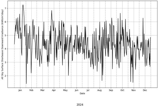
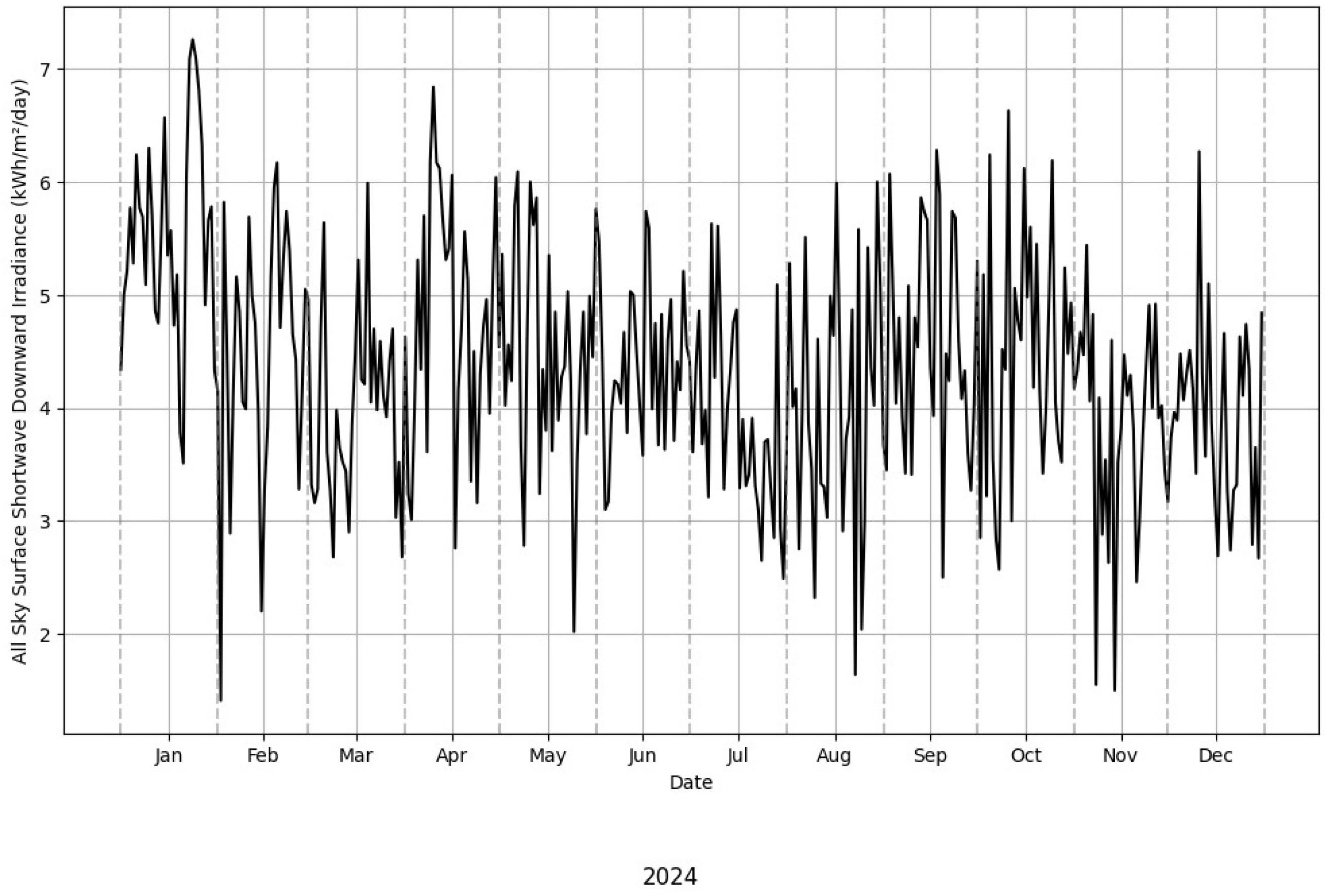
The full time series of 366 daily observations for the DT and ANN models is illustrated in Figure 2. During the year, the series of data shows extremely frequent and unpredictable movements, from rapid daily changes as opposed to a gentle seasonal pattern. In quantitative terms, solar irradiance for Neiva covers a wide dynamic range where 1.41 kWh/m²/day is the minimum value and 7.26 kWh/m²/day is the maximum value. This range is characteristic of the bimodal climatic regime of the Colombian Andean region, where marked drops in irradiance happen in the rainy months (April–May and October–November) as a result of a greater cloud layer, and periods with large irradiance (>6.0 kWh/m²/day) are recorded for the dry months (January–February and July–August). The non-linear meteorological dynamics are particularly important for predictive modeling because the extreme temporal variation insolar irradiance is the most important difficulty for reliable forecasting. Thus, modeling that captures both short-term variations and seasonal trends is vital to maximizing the utility of DT and ANN algorithms in day-to-day solar energy availability estimation.

Figure 2. Daily solar irradiance in Neiva (2.930079, −75.255650) from 1 January to 31 December 2024. Source: NASA Power-Prediction Of Worldwide Energy Resources (data); Google Colab (graph).

Table 1 corresponds to the exploratory data analysis initially performed to determine the maximum, minimum, and quartile values of the data used in this study. The average solar irradiance value was 4.370 kWh/m²/day, with a maximum value of up to 7.26 kWh/m²/day. The quartiles showed that 25% and 50% of days had irradiance values below 3.65 and 4.335 kWh/m²/day, respectively, while 75% exceeded 5.057 kWh/m²/day.

Table 1. Exploratory analysis of solar irradiance data from 1 January to 31 December 2024 in Neiva (2.930079, −75.255650).

Parameters	Month	Day	Solar Irradiance (kW-h/m2/day)
Count	12	366	366
Mean	6.513	15.756	4.370
Standard deviation	3.456	8.823	1.049
Minimum	1	1	1.410
25%	4	8	3.650
50%	7	16	4.335
75%	9.750	23	5.057
Maximum	12.0	31	7.26

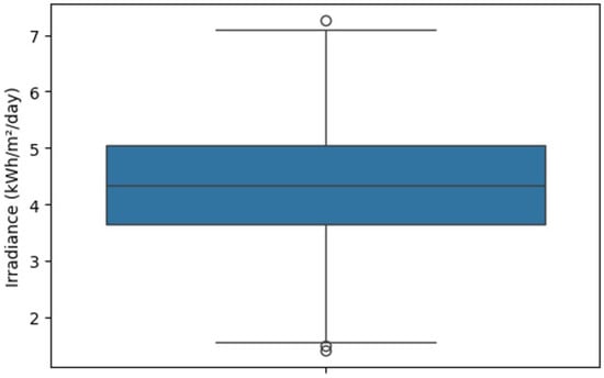
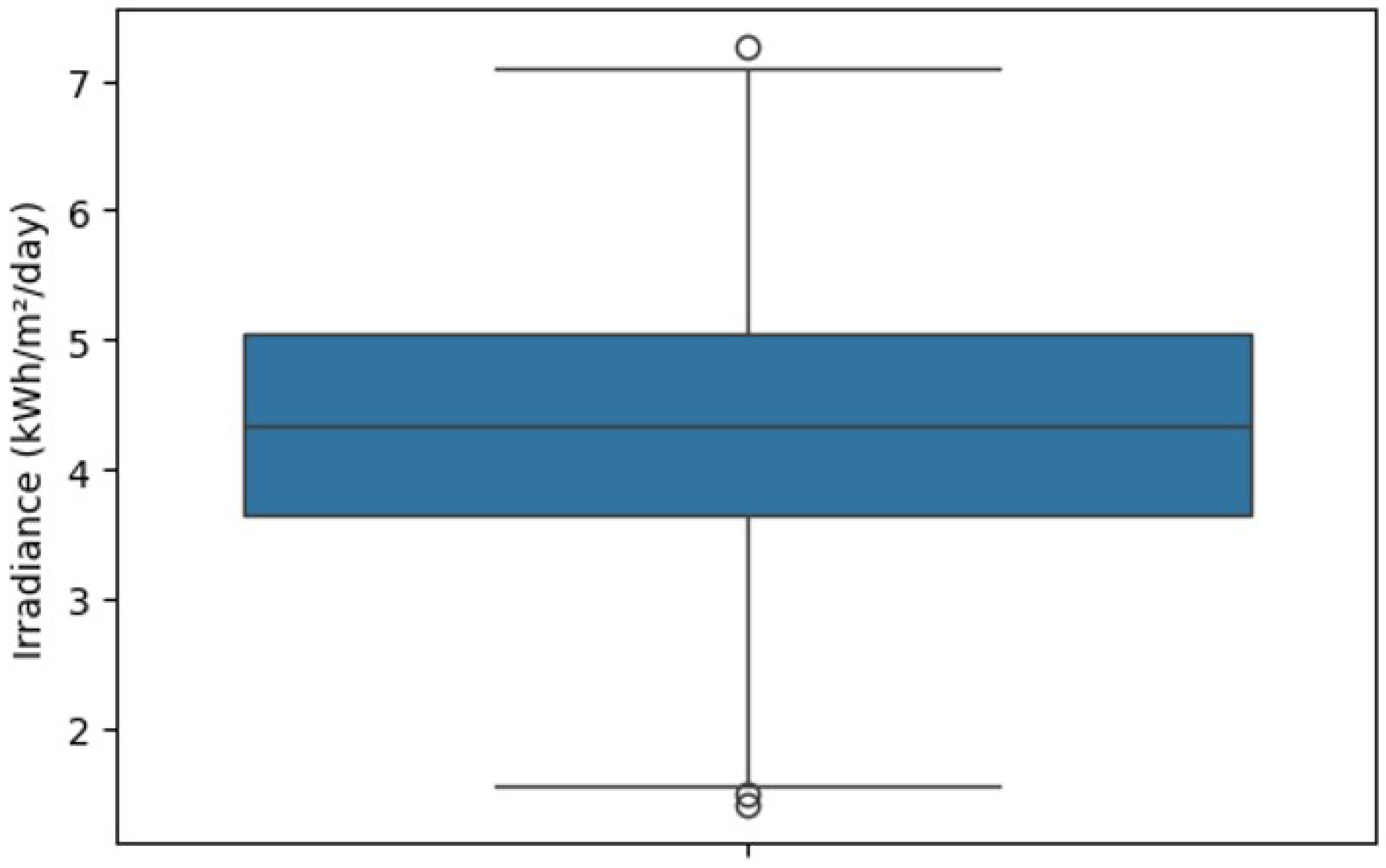
Figure 3 corresponds to the box plot product of the data processed in Google Colab. The median of the data, represented by the central line inside the box, and the quartiles that indicate the range in which the central 50% of the values are located are clearly observed. This figure reveals the presence of three outliers, represented by the points outside the whiskers of the box, suggesting that these values are significantly different from the rest of the data. It is important to note that the presence of these outliers can negatively affect the accuracy of the DT and ANN models evaluated in this study.

Figure 3. Box plot of daily solar irradiance recorded in Neiva (2.930079, −75.255650) from 1 January to 31 December 2024.

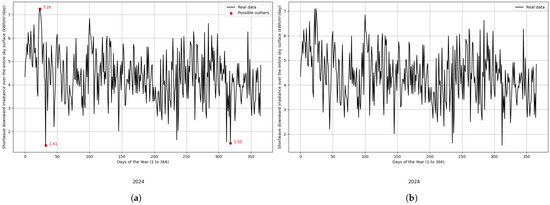
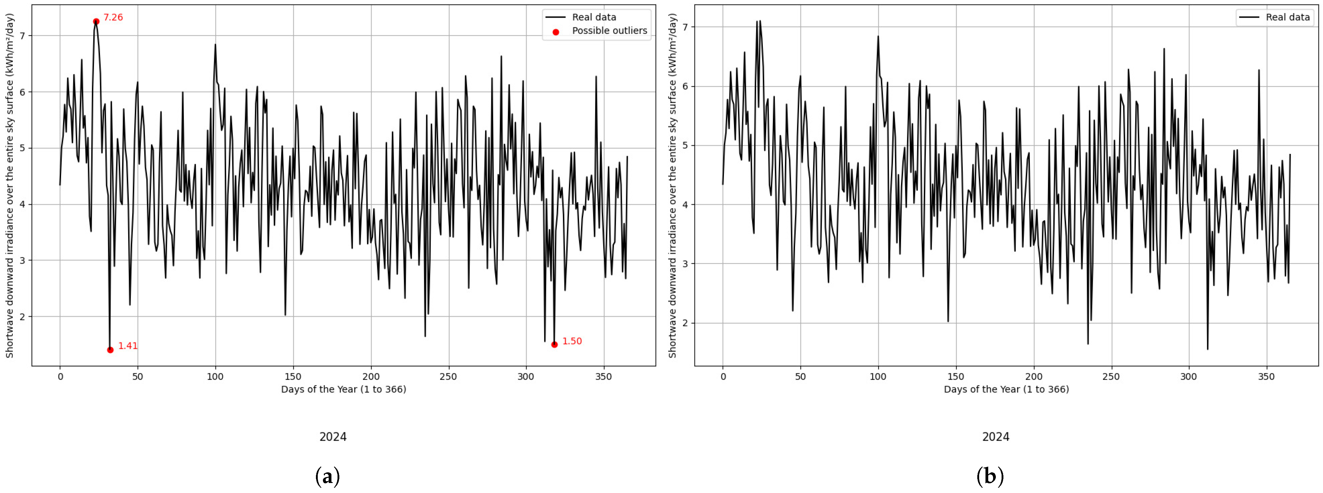
Taking into account what is reported in Figure 3 and the existence of three outliers, this work proposed two scenarios for the model training process. The first consisted of training the models under the original data, and the second replacing the three outliers (presented in Figure 3) using the moving-window median criterion to preserve the general shape of the data without introducing biases. This criterion consisted of replacing each outlier with the median of a window of five data points prior and five data points after the recording of each outlier. Table 2 presents the results considering both scenarios and the percentage change in the measurement metrics to determine the influence on the prediction fit under the two scenarios considered. On the other hand, the percentage error was determined using Equation (4). Figure 4 illustrates the trend in the data under these two scenarios.

$$\Delta \%=\left({\displaystyle \frac{\left|\mathrm{Case}\mathrm{value}1-\mathrm{Case}\mathrm{value}2\right|}{\mathrm{Case}\mathrm{value}1}}\right)\times 100\%$$

(4)

where the case 1 value represents the solar irradiance values obtained without the outlier treatment and the case 2 value corresponds to the values obtained after applying the outlier treatment using a moving-window median.

Table 2. Comparison of error metrics ($MAE$ and $RMSE$) between cases with and without outlier treatment.

Model	Metric	Case 1	Case 2	$\mathbf{\Delta }$%
Decision tree (DT)	Mean absolute error ($MAE$)	0.1399	0.1100	21.3720
Artificial neural network (ANN)	Mean absolute error ($MAE$)	0.7821	0.7729	1.1760
Decision tree (DT)	Root mean square error ($RMSE$)	0.5183	0.4401	15.0880
Artificial neural network (ANN)	Root mean square error $RMSE$	0.9767	0.9590	1.8120

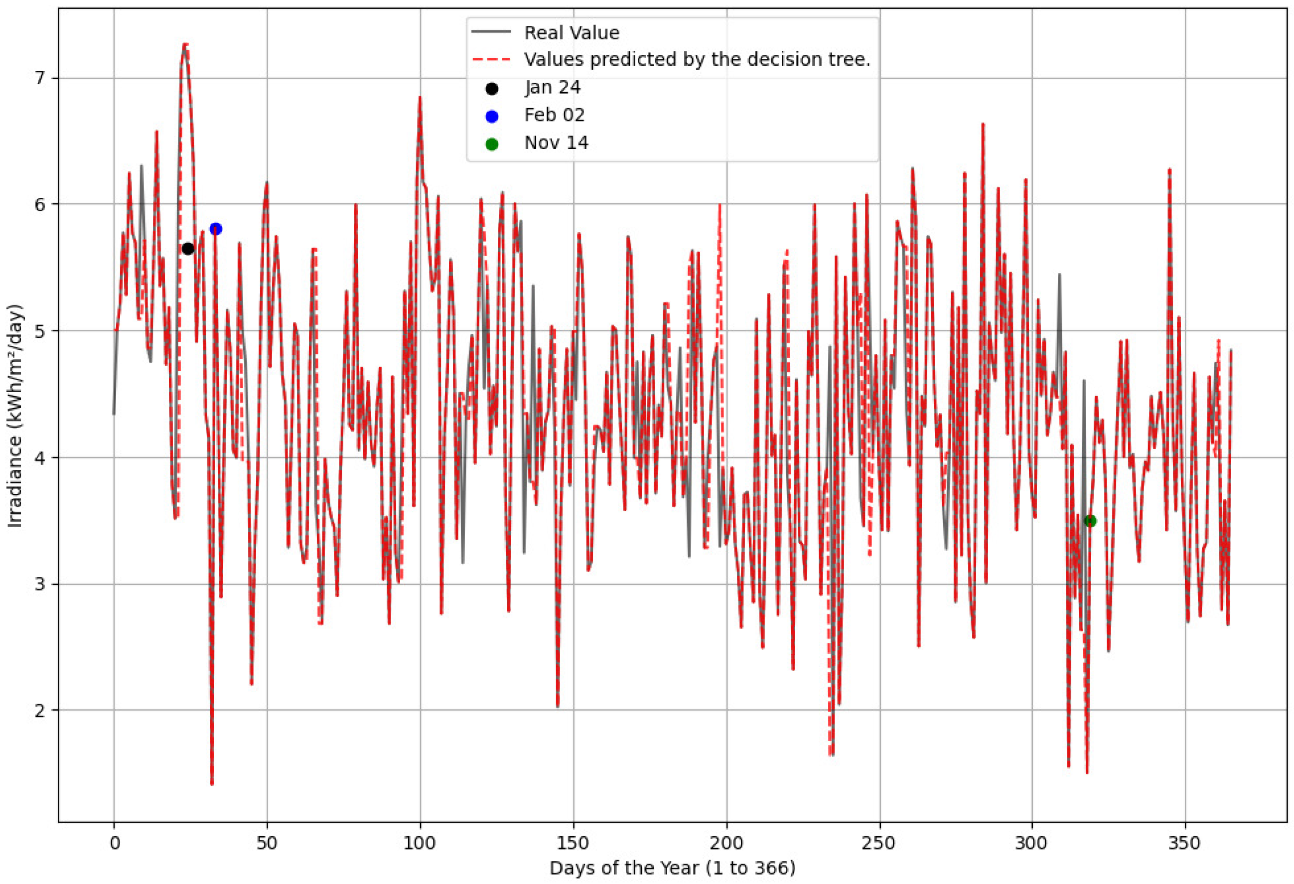
Figure 4. Solar irradiance during the observation window (366 days, corresponding to the 2024 calendar year): (a) response variable considering the original dataset, including the outliers identified in Figure 3 (24 January, 2 February, and 14 November); (b) response variable after applying a moving-window mean criterion to correct the three outlier points. Data correspond to the period from 1 January to 31 December 2024 in Neiva (2.930079, −75.255650).

In Figure 4a, three specific outliers are distinguished (7.26, 1.41, and 1.50 kWh/m²/day), corresponding to the anomalies initially detected in the box plot (Figure 3). To evaluate the impact of treating these values using the moving-window median criterion, Table 2 compares the error metrics ($MAE$ and $RMSE$) for the raw dataset (case 1) versus the treated dataset (case 2). This analysis shows that the preprocessing response is highly inconsistent with respect to how these models react. Concerning case 2, the DT model shows a considerable improvement of 21.37% in $MAE$ and 15.09% in $RMSE$ (compared to the ANN model, which demonstrates an insignificant boost ($\Delta <2\%$)). In addition, in terms of absolute performance, it is observed that the DT model in case 2 always significantly outperforms the ANN with an $MAE$ of 0.1100 compared to 0.7729. These data confirm that the outlier treatment is key to tuning the DT model’s accuracy. Therefore, based on the better data fit and reliability found, the dataset of case 2 is selected to train and evaluate the models in the future of this study.

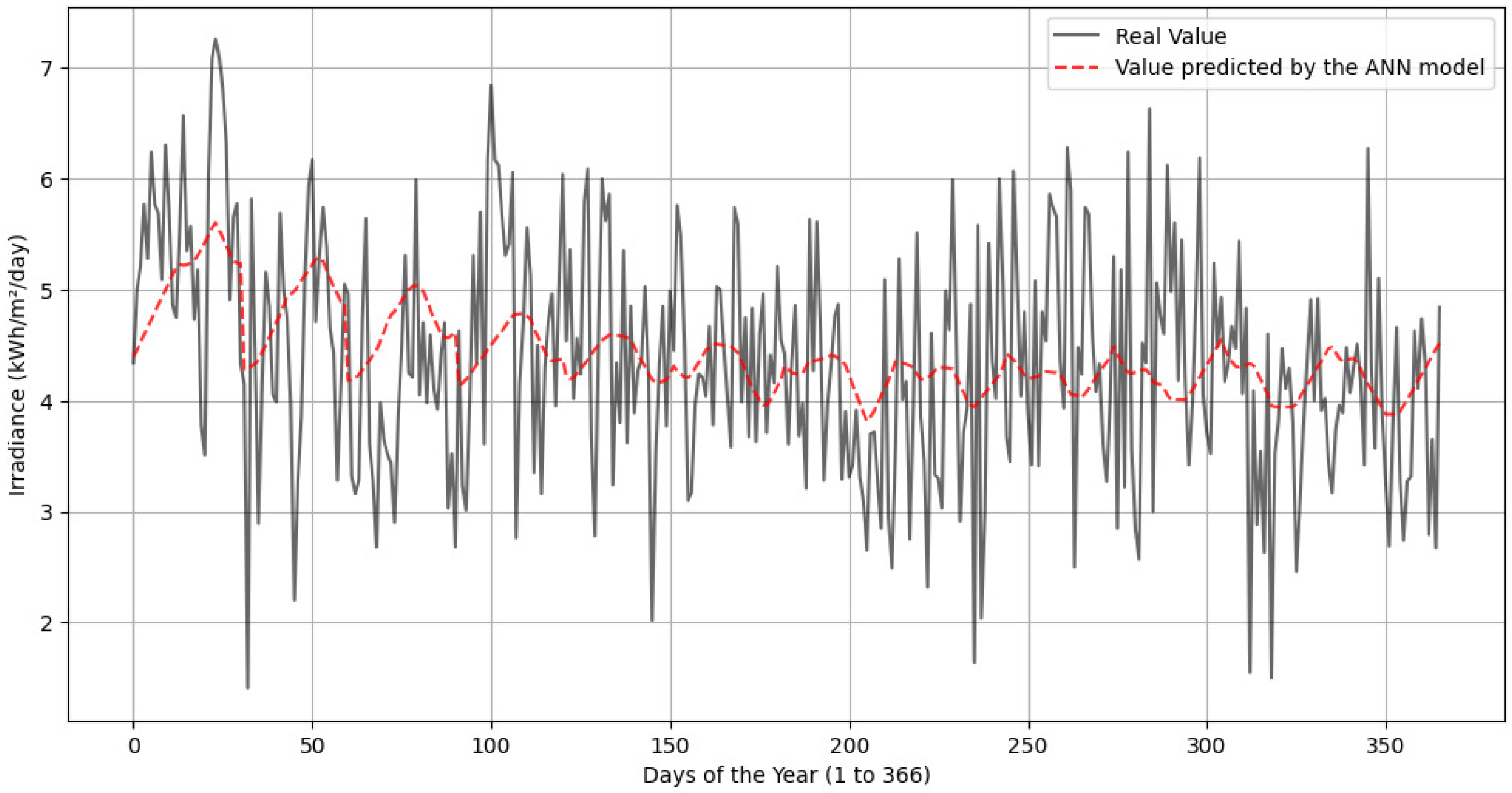
A comparison of the solar irradiance forecasting results (black line and red line) is summarized in Figure 5 and Figure 6 for the DT and ANN models, respectively. Figure 5 demonstrates the strong performance of the DT model in capturing the stochastic behavior of the solar irradiance, as it closely traces the daily high-frequency variation and correctly recreates the maximum radiation peaks as well as sharp drops in intensity due to intermittent cloud cover. Comparatively, Figure 6 suggests that an important limitation of the ANN model is its smoothness, which only expresses the central tendency or seasonal mean, but cannot predict the daily volatility. Therefore, Figure 5 clearly demonstrates the superiority of the DT model, which gives a good description of the dynamic operation of the resource and dramatically outperforms the generalization by the ANN model. Although both models attempt to predict the response variable, there are sizable differences in predictive capability. For objective estimation of the goodness-of-fit, $R^2$ is calculated for the best-performing runs for each model. The DT model produces an $R^2$ of 0.8798 (Iteration 3) which means that about 87.98% of the solar irradiance variance is accounted for effectively. In stark contrast, the ANN model yields a significantly lower $R^2$ of 0.7856 (Iteration 5). These results statistically confirm that the DT model provides a much more accurate representation of the dataset, making it the superior choice for describing the solar irradiance at the study site compared to the ANN approach.

Figure 5. Comparison between actual and predicted solar irradiance values for the DT model from 1 January to 31 December 2024 in Neiva (2.930079, −75.255650).

Figure 6. Comparison between actual and predicted solar irradiance values for the ANN model from 1 January to 31 December 2024 in Neiva (2.930079, −75.255650).

3.1. Evaluation of the Model Accuracy

Metrics, such as $RMSE$, $MAE$ and $R^2$, were used to evaluate the quality, level of precision and fit of each of the two models. In Table 3, the values obtained from the metrics for 10 consecutive iterations are compiled. The relevance of this study lies in the importance of AI in data prediction, since it allows for an approximation to be made as a tool that works as an artificial mind analogous to the human one. Thus, when it is consulted and asked to determine predicted data, it will not generate the same artificial values in all iterations, since the AI has the capacity to respond differentially.

Table 3. Error metrics ($RMSE$, $MAE$, and $R^2$) of the DT and ANN models for 10 iterations.

	DT Model			ANN Model
Iteration	$\mathit{RMSE}$	$\mathit{MAE}$	${\mathit{R}}^{\mathbf{2}}$	$\mathit{RMSE}$	$\mathit{MAE}$	${\mathit{R}}^{\mathbf{2}}$
1	0.4081	0.1031	0.8390	0.9593	0.1106	0.7703
2	0.4486	0.1173	0.8055	0.9514	0.1253	0.7643
3	0.3527	0.0895	0.8798	0.9561	0.1166	0.7723
4	0.5144	0.1278	0.7443	0.9568	0.1152	0.7699
5	0.3921	0.0912	0.8023	0.9701	0.1102	0.7856
6	0.4160	0.1096	0.8328	0.9573	0.1144	0.7700
7	0.4123	0.1146	0.8357	0.9627	0.1044	0.7775
8	0.3756	0.0849	0.8637	0.9589	0.1115	0.7688
9	0.4593	0.1160	0.7962	0.9676	0.0951	0.7749
10	0.3401	0.0936	0.8882	0.9505	0.1269	0.7679
Mean ($\overline{y}$)	0.4119	0.1048	0.8288	0.9591	0.1130	0.7722
Standard deviation ($\sigma$)	0.0522	0.0144	0.0434	0.0063	0.0093	0.0060

As can be observed from Table 3, with respect to the 10 iterations performed, the errors ($RMSE$ and $MAE$) are lower in the DT model, which is favorable for this algorithm and confirms the findings reported by Shorabeh et al. [40] and Singh et al. [41]. Additionally, $R^2$ tends to be closer to unity for the DT model, indicating that it possesses a greater ability to fit predicted versus actual values than that of the ANN model.

3.2. Statistical Analysis

The interpretation of residuals by statistical methods is key in determining the trustworthiness and stability of prediction models, especially in applications where data, such as daily solar irradiance, have relatively very high variability. In this context, residual evaluation for independence, normality, and homoscedasticity is performed to evaluate systematic errors, temporal dependencies, and predictive failure. This independence ensures that prediction errors are not correlated over time or between observations, which is particularly important in time series data where autocorrelation can be a sign of unmodeled temporal patterns. Normality of residuals signifies that the deviations from predicted values are random and symmetrical, thus validating statistical inferences and reliability of error statistics. Homoscedasticity (i.e., constant variation in the range of forecast values) therefore leads to improved performance for low and high irradiance to avoid biased predictions at extreme conditions. The analysis is performed at 5% significance, and the p-values are presented in parentheses, the first for the DT model and the second for the ANN model. Such residual diagnostics strengthen conventional performance metrics, including $RMSE$, $MAE$, and $R^2$, but more importantly enhance confidence in the generalization capability of the model and offer the possibility of further improvement in model formulations in the future. Still, careful residual analysis is indispensable to make the predictive models statistically sound; capable of representing stochastic and non-linear response behavior to solar irradiance; and suitable for practical use in energy planning, forecasting and optimization.

If a statistical test’s p-value is larger than a significance threshold value of 0.05, the null hypothesis is indeed not rejected and there is simply not enough support to show that the tested assumption is not met. In the residual study, a p-value greater than 0.05 indicates that the residuals do not deviate from the expected values under the null hypothesis. For independence tests, it indicates that there is not a statistically significant autocorrelation of errors. In turn, for normality tests, it informs that residuals follow an approximately normal distribution. Finally, for homoscedasticity tests, it indicates that error variances are approximately constant over the prediction range. Therefore, a p-value above 0.05 signals that the model does not tend to vary systematically from its statistical assumptions, and confidence in the stability of the error estimates and validity of the estimation for prediction and decision-making is confirmed.

3.2.1. Independence Analysis

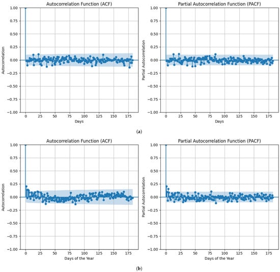
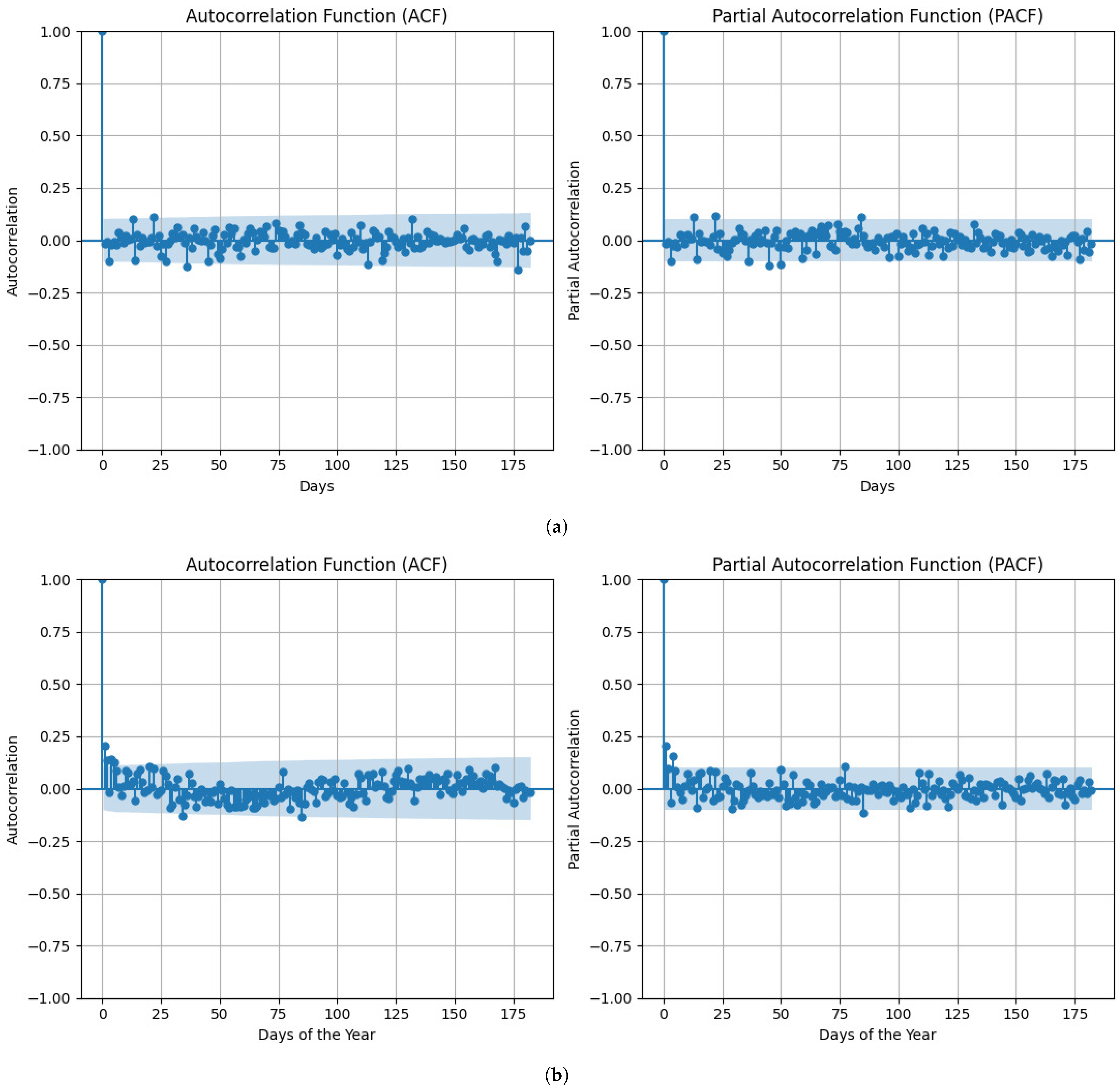
To verify the statistical reliability of the predictive models, statistical residuals were evaluated for their independence, where both quantitative metrics and graphical diagnostic analysis of residual independence were carried out at a 5% significance level. The test statistics were included in parentheses, in which the first value corresponded to the DT model, while the second one referred to the ANN model. To evaluate the presence of autocorrelation in the residuals, the Durbin–Watson and Ljung–Box tests were applied. The Durbin–Watson statistics were 1.9551 and 1.5502 for the DT and ANN models, respectively, which are close to the reference value of 2.0 and therefore suggest the absence of significant first-order autocorrelation. In addition, the Ljung–Box test results were $Q=0.068$, $df=1$, and $p=0.7903$ for the DT model and $Q=18.87$, $df=1$, and $p=1.7833$ for the ANN model, indicating that the null hypothesis of randomness could not be rejected ($p>0.05$). Graphically, this quantitative proof is supported by the autocorrelation (ACF) and Partial Autocorrelation (PACF) values for the DT (Figure 7a) and ANN (Figure 7b) models in Figure 7. As can be observed, correlation coefficients for almost all lags are mostly contained between the 95% confidence intervals (shaded regions). Additionally, these findings show that the residuals act as white noise, indicating that the resulting models have both fully captured the deterministic aspects of the solar irradiance and have not left temporal dependence patterns in the errors.

Figure 7. Autocorrelation (ACF) and parcial autocorrelation (PACF) graph for (a) DT model and (b) ANN model.

3.2.2. Normality Analysis

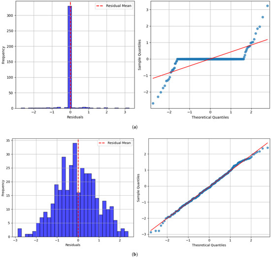
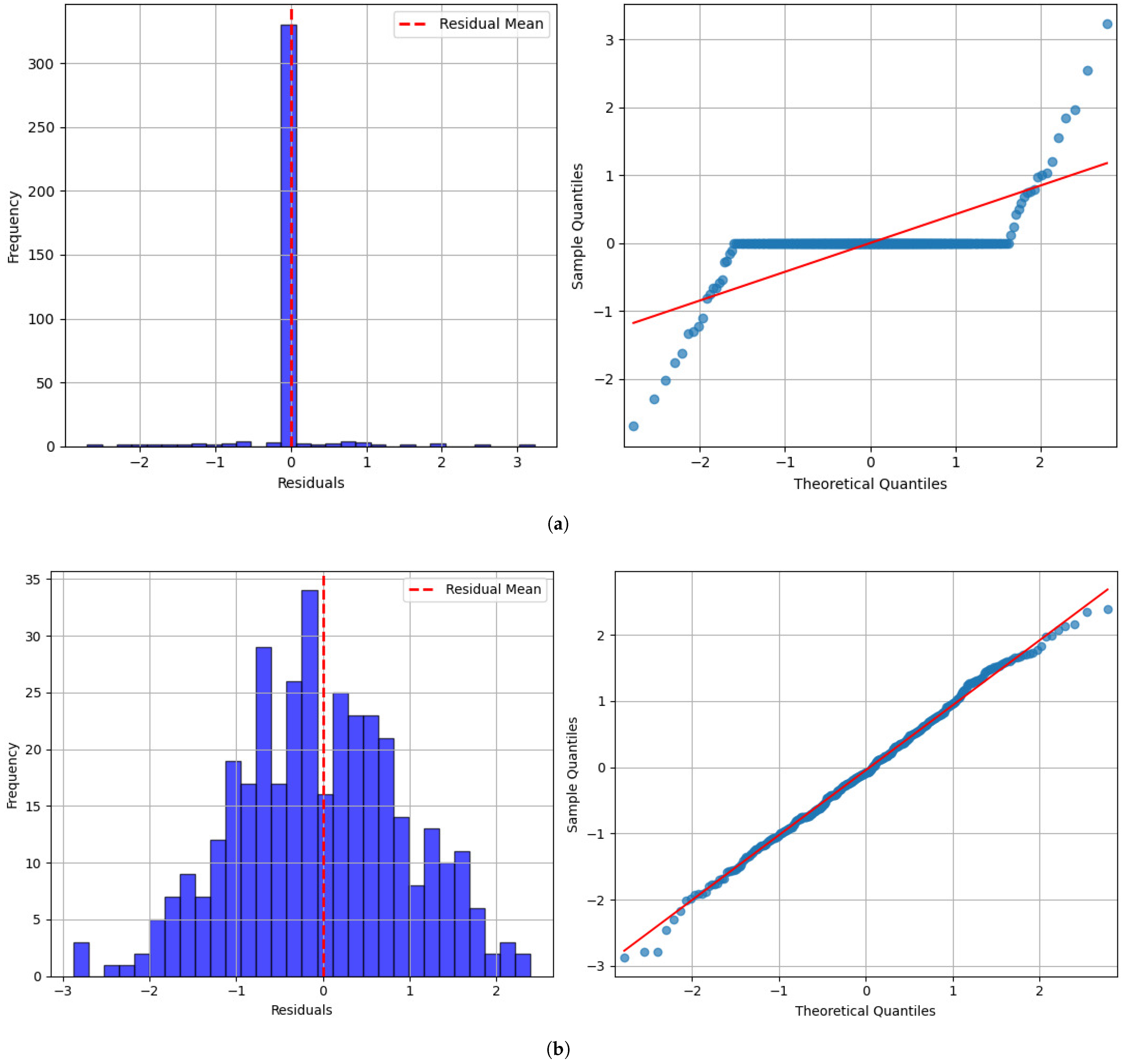
Normality tests were applied to evaluate the distribution of residuals for both predictive models. In particular, the Kolmogorov–Smirnov, Jarque–Bera, and Shapiro–Wilk tests were performed. The results were as follows: Kolmogorov–Smirnov test (DT: $D=0.4835$, $p=0.0000$; ANN: $D=0.0269$, $p=0.9691$), Jarque–Bera test (DT: $JB=12518.6625$, $p=0.0000$; ANN: $JB=1.6651$, $p=0.7201$), and Shapiro–Wilk test (DT: $W=0.3321$, $p=0.0000$; ANN: $W=0.9966$, $p=0.6620$). These results indicated that the assumption of normality was only satisfied for the ANN model ($p>0.05$), which was also visually supported by the residual distribution shown in Figure 8. The ANN residuals were symmetric from the Gaussian histogram to the diagonal corresponding to the Q-Q plot, confirming an unbiased distribution, as illustrated in Figure 8b. On the contrary, DT (Figure 8a) presented a leptokurtic histogram and discrete, step-like structure in the Q-Q plot. While the DT residuals did not follow a normal distribution (due to its classification as a non-parametric model), this is an inherent property of regression trees, supporting the improved statistical stability of the ANN for model evaluation.

Figure 8. Frequency distribution plot and normal probability curve for (a) DT model and (b) ANN model.

It is highlighted that the observed non-normality of DT residuals (p-value < 0.05) is an expected behavior, valid for modeling, and is not a reason to invalidate its ability to make predictions. In contrast to the ANN model, the DTs are non-parametric algorithms that approximate the target function with a piecewise constant structure. This produces discrete predictions that naturally induce a multimodal or leptokurtic residual distribution, as evidenced by the step-like pattern depicted on the Q-Q plot (Figure 8a). Thus, although the ANN model performs relatively well in terms of its statistical superiority (through normality assumption), the DT model should be considered as a valid estimation tool, and performance evaluation should be conducted on error metrics ($RMSE$, $MAE$) rather than simply on normality.

3.2.3. Homoscedasticity Analysis

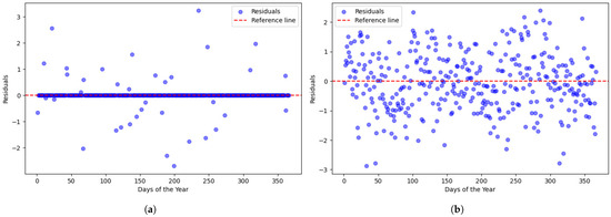
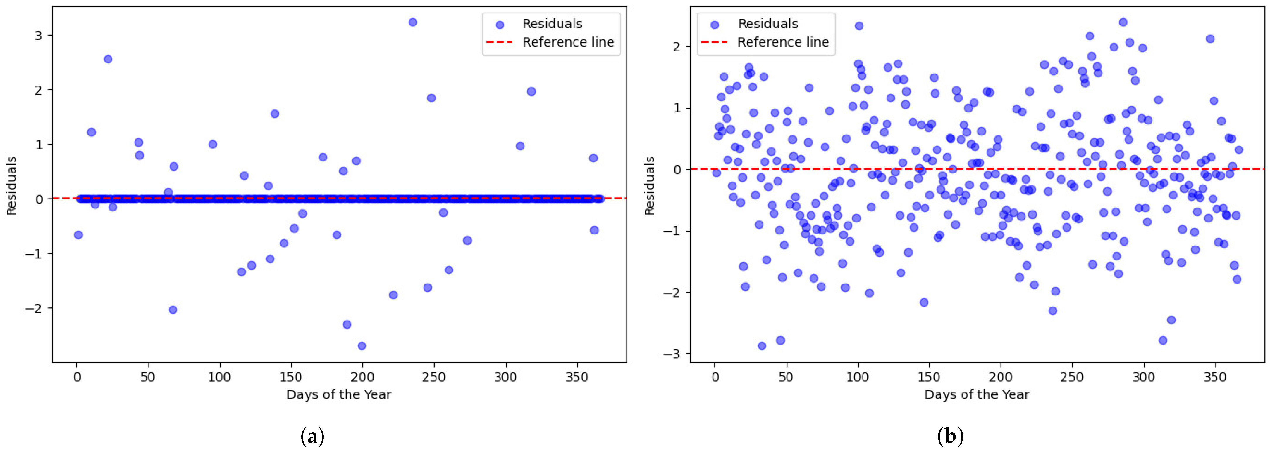
To assess the assumption of homoscedasticity (i.e., constant variance in residuals), the Bartlett, Breusch–Pagan, and Levene tests are performed for both models. The results are as follows: Bartlett’s test (DT: ${\chi }^2=195.599$, $df=1$, $p=0.0000$; ANN: ${\chi }^2=1.4049$, $df=1$, $p=0.2499$), Breusch–Pagan test (DT: $BP=4.2934$, $df=2$, $p=0.0383$; ANN: $BP=0.3418$, $df=2$, $p=0.6337$), and Levene’s test (DT: $F=314.1049$, $d{f}_1=X$, $d{f}_2=366$, $p=0.0000$; ANN: $F=1.3985$, $d{f}_1=1$, $d{f}_2=366$, $p=0.2407$). The results show that the homoscedasticity assumption is satisfied exclusively by the ANN model ($p>0.05$), a point further corroborated graphically in Figure 9. As can be seen from Figure 9b, the ANN residuals exhibit a random, uniform dispersion around the zero reference line throughout the year, without displaying funnel shapes or systematic trends. This validates that the error variance is independent of the season. On the other hand, the DT model displays a large number of residuals that collapse onto the zero axis with sporadic outliers (Figure 9a), representing heteroscedasticity (due to discrete DT predictions), which seems to be common among the large population of tree predictions in terms of the model itself. Thus, the ANN model is found to be statistically more robust and stable than the heuristic version.

Figure 9. Scatter plot of residuals versus predicted values for (a) DT model and (b) ANN model.

Additionally, the DT model does not satisfy homoscedasticity (p < 0.05) and proves to be heteroscedastic. This result is in line with the operational mechanics of regression trees, which break up the input space into “leaves” with different statistical properties. In contrast to linear models where heteroscedasticity implies inefficient estimators being employed, the DT models handle varying error variance by producing deeper splits in high-variance areas to reduce impurity. Therefore, while the lack of homoscedasticity indicates that the model’s uncertainty varies across the dataset (e.g., higher prediction intervals during transitional weather months), it does not compromise the accuracy of the point forecasts, as evidenced by the performance metrics ($RMSE$, $MAE$).

Although the statistical analysis of both models reveals that the assumption of independence has been met, the normality and homoscedasticity test of the DT model is still under consideration, which does not favor the statement that the distribution of the response variable is close to the normal distribution and that the fit of the model to the data is reliable. However, according to Hoekstra et al. [59], in ML models, such as DT or neural networks, the focus is on predictive accuracy rather than on the validity of these classical inferential statistical assumptions, so that failure to meet the assumptions of normality and homoscedasticity in the residuals does not invalidate the predictive models. As reported by Hoekstra et al., these statistical techniques do not require strict assumptions and turn out to be more flexible in supervised learning. Therefore, these models do not require the user to specify the form of the relationship between the predictors and the response variable, as, for example, a linear regression model does [60]. Thus, in this work, a transformation of the variable is not performed to comply with the assumptions as would be done in a regression model.

3.3. Comparative Analysis

Quantitative assessment of the models has an obvious value-based trade-off between statistical compliance and predictive performance. As discussed in the previous sections, the ANN model meets the normality (Figure 8b) and homoscedasticity (Figure 9b) assumptions, exhibiting superior statistical properties. Thus, in this case, the ANN model is a robust, well-behaved error distribution estimator and is statistically unbiased. Nevertheless, as noted within Table 3, such kinds of statistical rigor do not translate into improved forecasting on this dataset. On the contrary, the DT model performs significantly better than the ANN approach in all 10 iterations, with an average $RMSE$ much lower (∼0.41) under a scenario with ANN (∼0.96) and an upper determination coefficient ($R^2$ up to $0.88$). This indicates a heuristic non-parametric property of DT (i.e., its ability to split feature space into discrete hyper-rectangles) that is better suited to model the sudden, stochastic deviations in solar irradiance in Neiva, despite the latter being observed earlier. However, even though the DT model does not meet the tests of normality and homoscedasticity because of the discrete structure of the output (step-like residuals), such a statistical violation allows the model to respond more aggressively to sudden shifts in weather. Conversely, the ANN, due to its smooth and continuous approximation, seems to over-smooth the data, preventing it from encapsulating the extreme peak–valleys of the irradiance profile that correspond to higher $RMSE$ values. Hence, from the end of the engineering concern for minimizing forecasting error, the DT model is selected as superior by emphasizing raw accuracy rather than theoretical statistical purity.

While the DT model performed better than the ANN model in terms of prediction performance for both evaluation metrics, the ANN model had smoother prediction curves. This characteristic may be advantageous in applications related to long-term energy planning, where capturing general trends in solar resource availability can be more relevant than reproducing short-term daily fluctuations. Specifically, DT models can have relatively higher accuracy in capturing daily variability. However, the ANN-based approach can be more stable in expressing the temporal dynamics of solar irradiance, which could be beneficial for both strategic planning and energy management applications. It is for these reasons that, according to Aouidad and Bouhelal (2024), daily solar irradiance was a key parameter to be analyzed, in light of the fact that variations in solar radiation may lead to interferences in the power supply grid, which is also well-demonstrated in their work [65]. Energy is produced daily in homes, businesses and industries, where the energy infrastructure is grid-connected, and on-site generation occurs for rural and isolated areas and non-SIN-integrated energy communities. From the observation by Trull et al. (2025), time series-only models perform poorly. This supports the conclusion that the DT model performed better than the ANN model when subjected to fluctuating daily patterns and in particular to daily shifts [66].

The difference between the predictive performance of DT and ANN models can certainly be considered useful in practical applications of solar resource-based energy planning. In the case of operational applications, because it is mandatory to consider the daily variation in solar irradiance as having a direct impact on the operational management of power systems, the DT model can best model the daily variability in solar irradiance compared to the ANN model. For example, generation scheduling, reserve management, and the operation of grids with high solar penetration all rely on prediction to track day-to-day changes which result in better decisions and less uncertainty in operations [67].

However, the ANN model provides smoother predictions, showing that it is more successful in capturing the general conditions of the solar resource by avoiding noise and short-term fluctuations. This functionality is useful for long-term and strategic planning scenarios, such as evaluating the energy potential of a site, sizing PV systems or conducting feasibility studies for solar projects, as it tends to be more useful for tracking trends than daily variations [67].

As a result, the most appropriate model selection depends on the intended application. DT models might fit better for operation, depending on a good approximation of daily solar variations, whereas ANN models would be more suitable to plan and carry out strategic analyses where a more stable representation of trends is found.

This improved perspective also underscores that these are an important factor of difference in some case scenarios in solar energy systems. In terms of applications, because the generation of PV varies drastically in response to an evolution of ambient atmosphere (e.g., cloud cover, humidity, and incoming radiation), DT-based models serve as a great utility model. Modeling these shifts correctly has critical ramifications for generation scheduling, reserve provisioning, and supply and demand balancing in renewable-dominated systems. Furthermore, the models are extremely useful in smart grid operation, real-time energy management, and energy storage system optimization, as the variability prediction is significant for the most energy-efficient charge and discharge design.

ANN models are also considered for modeling complex non-linear relationships between meteorological variables and solar generation in the literature. Such smooth outputs are well-suited for evaluating solar resources, planning and designing PV systems and sizing them, regional energy planning, and estimating annual energy yield for financial and investment analyses. As in these cases, it is more critical to capture stable and generalizable patterns than to reproduce high frequency variability [67].

Finally, incorporating additional meteorological variables from the NP database could provide deeper insights into the sensitivity of the models and their predictive performance. Although such an analysis was beyond the scope of the present study, it represents a promising direction for future research. Exploring the influence of a broader set of atmospheric parameters may help to better understand the relationships between environmental conditions and model accuracy, potentially contributing to the development of more robust and reliable forecasting approaches.

4. Conclusions

Throughout the current work, it could be inferred that the DT model presented a better fit in the prediction of daily solar irradiance, outperforming the ANN model in all the evaluated metrics ($RMSE$, $MAE$, and $R^2$, where the DT model reached a maximum value of $R^2$ of 0.8882 compared to 0.7679 achieved in the ANN model (10th iteration). Additionally, the $MAE$ and $RMSE$ under the outlier treatment proved to be beneficial for the models, which demonstrates the importance of preprocessing the information prior to model training. In this work, it was possible to reflect an application of supervised learning for the prediction of solar energy data adapted to a Colombian context, favoring the incorporation of AI in non-conventional renewable energy sources, where information on the prediction of solar irradiance is still scarce in this country. Nevertheless, explorations of techniques and new ML models are suggested to be reviewed, as well as to use meteorological data from locations with great solar energy potential in Colombian departments such as La Guajira, Tolima and Atlántico. Finally, the consolidation of these types of studies can contribute significantly to regional and national energy planning, especially in intermediate cities with high solar irradiation and growing energy demand.

References

- Saleh, H.M.; Hassan, A.I. The challenges of sustainable energy transition: A focus on renewable energy. Appl. Chem. Eng. 2024, 7, 2084. [Google Scholar] [CrossRef] [Scilit]
- Balcerzak, A.P.; Uddin, G.S.; Dutta, A.; Pietrzak, M.B.; Iglinski, B. Energy mix management: A new look at the utilization of renewable sources from the perspective of the global energy transition. Equilibrium 2024, 19, 379–390. [Google Scholar] [CrossRef] [Scilit]
- Plazas-Niño, F.A.; Yeganyan, R.; Cannone, C.; Howells, M.; Quirós-Tortós, J. Informing sustainable energy policy in developing countries: An assessment of decarbonization pathways in Colombia using open energy system optimization modelling. Energy Strategy Rev. 2023, 50, 101226. [Google Scholar] [CrossRef] [Scilit]
- Olbrich, S.; Bauknecht, D.; Späth, P. Policy mixes for net-zero energy transitions: Insights from energy sector integration in Germany. Energy Res. Soc. Sci. 2024, 118, 103822. [Google Scholar] [CrossRef] [Scilit]
- Bera, M.; Das, S.; Garai, S.; Dutta, S.; Choudhury, M.R.; Tripathi, S.; Chatterjee, G. Advancing energy efficiency: Innovative technologies and strategic measures for achieving net zero emissions. Carbon Footprints 2025, 4, 3. [Google Scholar] [CrossRef] [Scilit]
- Wu, Y.-H.; Lee, T.-C. Designing a cost-effective policy mix for transition toward net-zero emissions: A case study of the mid-term plan by 2035 of Taiwan. Carbon Manag. 2024, 15, 2379545. [Google Scholar] [CrossRef] [Scilit]
- Aminzadegan, S.; Shahriari, M.; Mehranfar, F.; Abramović, B. Factors affecting the emission of pollutants in different types of transportation: A literature review. Energy Rep. 2022, 8, 2508–2529. [Google Scholar] [CrossRef] [Scilit]
- Sagastume Gutiérrez, A.; Cabello Eras, J.J.; Otero Meza, D.D. The Energy Transition in Colombia: Government Projections and Realistic Scenarios. Clean Technol. 2025, 7, 96. [Google Scholar] [CrossRef] [Scilit]
- Rumbayan, M.; Kindangen, J.; Sambul, A.; Sompie, S.; Cross, J. Solar energy implementation in rural communities and its contributions to SDGs: A systematic literature review. Unconv. Resour. 2025, 6, 100180. [Google Scholar] [CrossRef] [Scilit]
- Bhatia, S.C. Solar radiations. In Advanced Renewable Energy Systems; WPI Publishing: New York, NY, USA, 2014; pp. 32–67. [Google Scholar]
- Mukherjee, P.K. Quality Evaluation of Herbal Medicines: Challenges and Opportunities. In Quality Control and Evaluation of Herbal Drugs; Elsevier: Amsterdam, The Netherlands, 2019; pp. 53–77. [Google Scholar]
- Kopp, G. Solar irradiance measurements. Living Rev. Sol. Phys. 2025, 22, 1. [Google Scholar] [CrossRef] [Scilit]
- Trenberth, K.E.; Fasullo, J.T.; Balmaseda, M.A. Earth’s energy imbalance. J. Clim. 2014, 27, 3129–3144. [Google Scholar] [CrossRef] [Scilit]
- Kim, J.; Kim, E.; Jung, S.; Kim, M.; Kim, B.; Kim, S. Improved Surface Solar Irradiation Estimation Using Satellite Data and Feature Engineering. Remote Sens. 2024, 17, 65. [Google Scholar] [CrossRef] [Scilit]
- Radzi, P.N.L.M.; Mekhilef, S.; Shah, N.; Akhter, M.N.; Hassani, S.; Albaker, A.; Wahyudie, A. Performance evaluation and degradation analysis of grid connected photovoltaic systems for energy efficient buildings in tropical climates. Sci. Rep. 2025, 15, 39103. [Google Scholar] [CrossRef] [Scilit] [PubMed]
- Rao, R.D.D.; Gowda, B.S. Technical and economic feasibility analysis of 1 kW rooftop solar photovoltaic system for Mysuru, Karnataka, India. J. Therm. Eng. 2025, 11, 1507–1519. [Google Scholar]
- Eras, J.J.C.; Morejón, M.B.; Gutiérrez, A.S.; García, A.P.; Ulloa, M.C.; Martínez, F.J.R.; Rueda-Bayona, J.G. A look to the electricity generation from non-conventional renewable energy sources in Colombia. Int. J. Energy Econ. Policy 2019, 9, 15–25. [Google Scholar] [CrossRef] [Scilit]
- Rubio-Clemente, A.; Chica, E.; Penuela, G.A. Photovoltaic array for powering advanced oxidation processes: Sizing, application and investment costs for the degradation of a mixture of anthracene and benzo[a]pyrene in natural water by the UV/H2O2 system. J. Environ. Chem. Eng. 2018, 6, 2751–2761. [Google Scholar] [CrossRef] [Scilit]
- Itskos, G.; Nikolopoulos, N.; Kourkoumpas, D.-S.; Koutsianos, A.; Violidakis, I.; Drosatos, P.; Grammelis, P. Energy and the Environment. In Environment and Development; Elsevier: Amsterdam, The Netherlands, 2016; pp. 363–452. [Google Scholar]
- Ukoba, K.; Yoro, K.O.; Eterigho-Ikelegbe, O.; Ibegbulam, C.; Jen, T.-C. Adaptation of solar energy in the Global South: Prospects, challenges and opportunities. Heliyon 2024, 10, e28009. [Google Scholar] [CrossRef] [Scilit]
- Ellis, G.; Schneider, N.; Wüstenhagen, R. Dynamics of social acceptance of renewable energy: An introduction to the concept. Energy Policy 2023, 181, 113706. [Google Scholar] [CrossRef] [Scilit]
- Chatterjee, S.; Khan, P.W.; Byun, Y.-C. Recent advances and applications of machine learning in the variable renewable energy sector. Energy Rep. 2024, 12, 5044–5065. [Google Scholar] [CrossRef] [Scilit]
- Zhou, Y.; Liu, Y.; Wang, D.; Liu, X.; Wang, Y. A review on global solar radiation prediction with machine learning models in a comprehensive perspective. Energy Convers. Manag. 2021, 235, 113960. [Google Scholar] [CrossRef] [Scilit]
- Apeh, O.O.; Nwulu, N.I. Machine learning approach for short- and long-term global solar irradiance prediction. J. Environ. Earth Sci. 2025, 7, 321–342. [Google Scholar] [CrossRef] [Scilit]
- Yang, Y.; Huang, F.; Kang, S. Mechanism of Penetration Rate Improvement in Hot Dry Rock Under the Coupling of Impact Load and Confining Pressure Release. Reserv. Sci. 2026, 2, 52–64. [Google Scholar] [CrossRef] [Scilit]
- Tahir, M.U.; Guo, S. Preliminary Investigation of Fracture Behavior during Carbon Dioxide Fracturing of Natural Hydrogen Reservoir with Hard-Core Imperfections. Reserv. Sci. 2026, 2, 34–51. [Google Scholar] [CrossRef] [Scilit]
- Allal, Z.; Noura, H.N.; Chahine, K. Machine learning algorithms for solar irradiance prediction: A recent comparative study. e-Prime-Adv. Electr. Eng. Electron. Energy 2024, 7, 100453. [Google Scholar] [CrossRef] [Scilit]
- Markovics, D.; Mayer, M.J. Comparison of machine learning methods for photovoltaic power forecasting based on numerical weather prediction. Renew. Sustain. Energy Rev. 2022, 161, 112364. [Google Scholar] [CrossRef] [Scilit]
- Pandžić, F.; Capuder, T. Advances in short-term solar forecasting: A review and benchmark of machine learning methods and relevant data sources. Energies 2023, 17, 97. [Google Scholar] [CrossRef] [Scilit]
- Neuer, M.J. Machine Learning for Engineers: Introduction to Physics-Informed, Explainable Learning Methods for AI in Engineering Applications; Springer Nature: Berlin/Heidelberg, Germany, 2024. [Google Scholar]
- Zhang, J.; Li, J. Machine learning algorithm for cognitive engine. In Spatial Cognitive Engine Technology; Academic Press: Cambridge, MA, USA, 2023; pp. 169–185. [Google Scholar]
- Wang, L.; Zhang, Z.; Zhang, X.; Zhou, X.; Wang, P.; Zheng, Y. A Deep-forest based approach for detecting fraudulent online transaction. Adv. Comput. 2021, 120, 1–38. [Google Scholar]
- Ortiz, D.; Migueis, V.; Leal, V.; Knox-Hayes, J.; Chun, J. Analysis of renewable energy policies through decision trees. Sustainability 2022, 14, 7720. [Google Scholar] [CrossRef] [Scilit]
- Chen, M.; Claramunt, C.; Cöltekin, A.; Liu, X.; Peng, P.; Robinson, A.C.; Wang, D.; Strobl, J.; Wilson, J.P.; Batty, M. Artificial intelligence and visual analytics in geographical space and cyberspace: Research opportunities and challenges. Earth-Sci. Rev. 2023, 241, 104438. [Google Scholar] [CrossRef] [Scilit]
- Battista, D.; Mangone, E. Technological Culture and Politics: Artificial Intelligence as the New Frontier of Political Communication. Societies 2025, 15, 75. [Google Scholar] [CrossRef] [Scilit]
- Allal, Z.; Noura, H.N.; Salman, O.; Chahine, K. Machine learning solutions for renewable energy systems: Applications, challenges, limitations, and future directions. J. Environ. Manag. 2024, 354, 120392. [Google Scholar] [CrossRef] [Scilit]
- Ajibade, S.-S.M.; Flores, D.D.C.; Ayaz, M.; Dodo, Y.A.; Areche, F.O.; Adediran, A.O.; Oyebode, O.J.; Dayupay, J.P. Application of machine learning in renewable energy: A bibliometric analysis of a decade. In 2023 IEEE International Conference on Automatic Control and Intelligent Systems (I2CACIS); IEEE: New York, NY, USA, 2023; pp. 173–179. [Google Scholar]
- Gutiérrez, L.; Patiño, J.; Duque-Grisales, E. A comparison of the performance of supervised learning algorithms for solar power prediction. Energies 2021, 14, 4424. [Google Scholar] [CrossRef] [Scilit]
- Sahin, G.; Isik, G.; van Sark, W.G.J.H.M. Predictive modeling of PV solar power plant efficiency considering weather conditions: A comparative analysis of artificial neural networks and multiple linear regression. Energy Rep. 2023, 10, 2837–2849. [Google Scholar] [CrossRef] [Scilit]
- Shorabeh, S.N.; Samany, N.N.; Minaei, F.; Firozjaei, H.K.; Homaee, M.; Boloorani, D.A. A decision model based on decision tree and particle swarm optimization algorithms to identify optimal locations for solar power plants construction in Iran. Renew. Energy 2022, 187, 56–67. [Google Scholar] [CrossRef] [Scilit]
- Singh, N.; Jena, S.; Panigrahi, C.K. A novel application of Decision Tree classifier in solar irradiance prediction. Mater. Today Proc. 2022, 58, 316–323. [Google Scholar] [CrossRef] [Scilit]
- Gupta, A.; Bansal, A.; Roy, K. Solar energy prediction using decision tree regressor. In 2021 5th International Conference on Intelligent Computing and Control Systems (ICICCS); IEEE: New York, NY, USA, 2021; pp. 489–495. [Google Scholar]
- Kassim, N.M.; Santhiran, S.; Alkahtani, A.A.; Islam, M.A.; Tiong, S.K.; Yusof, M.Y.M.; Amin, N. An adaptive decision tree regression modeling for the output power of large-scale solar (LSS) farm forecasting. Sustainability 2023, 15, 13521. [Google Scholar] [CrossRef] [Scilit]
- Toylan, H. Solar irradiance prediction using bagging decision tree-based machine learning. Kirklareli Univ. J. Eng. Sci. 2022, 8, 15–24. [Google Scholar] [CrossRef] [Scilit]
- Amer, H.N.; Dahlan, N.Y.; Azmi, A.M.; Latip, M.F.A.; Onn, M.S.; Tumian, A. Solar power prediction based on Artificial Neural Network guided by feature selection for Large-scale Solar Photovoltaic Plant. Energy Rep. 2023, 9, 262–266. [Google Scholar] [CrossRef] [Scilit]
- Barrera, J.M.; Reina, A.; Maté, A.; Trujillo, J.C. Solar energy prediction model based on artificial neural networks and open data. Sustainability 2020, 12, 6915. [Google Scholar] [CrossRef] [Scilit]
- Iglesias-Sanfeliz Cubero, Í.M.; Meana-Fernández, A.; Ríos-Fernández, J.C.; Ackermann, T.; Gutiérrez-Trashorras, A.J. Analysis of neural networks used by artificial intelligence in the energy transition with renewable energies. Appl. Sci. 2023, 14, 389. [Google Scholar] [CrossRef] [Scilit]
- Sanchez-Lopez, J.E.; Solís-García, J.; Riquelme, J.C. Semi-real-time decision tree ensemble algorithms for very short-term solar irradiance forecasting. Int. J. Electr. Power Energy Syst. 2024, 158, 109947. [Google Scholar] [CrossRef] [Scilit]
- Essam, Y.; Ahmed, A.N.; Ramli, R.; Chau, K.-W.; Ibrahim, M.S.I.; Sherif, M.; Sefelnasr, A.; El-Shafie, A. Investigating photovoltaic solar power output forecasting using machine learning algorithms. Eng. Appl. Comput. Fluid Mech. 2022, 16, 2002–2034. [Google Scholar] [CrossRef] [Scilit]
- IDEAM. Atlas Climatológico de Colombia. Instituto de Hidrología, Meteorología y Estudios Ambientales (IDEAM). Available online: http://www.ideam.gov.co/documents/21021/418894/Temperatura+Media%2C+M%C3%A1xima+y+M%C3%ADnima.pdf/1c72e73e-3f07-4a6c-b900-48ff1442f5e2 (accessed on 13 June 2025).
- La República. Ideam Revela Récords de Temperatura en Más de 20 Ciudades Durante Inicio de Año. Diario La República. Available online: https://www.larepublica.co/economia/records-de-temperatura-en-mas-de-20-ciudades-3789361 (accessed on 5 February 2025).
- Kaldellis, J.; Zafirakis, D. Experimental investigation of the optimum photovoltaic panels’ tilt angle during the summer period. Energy 2012, 38, 305–314. [Google Scholar] [CrossRef] [Scilit]
- Rehman, N.; Uzair, M. Optimizing the inclined field for solar photovoltaic arrays. Renew. Energy 2020, 153, 280–289. [Google Scholar] [CrossRef] [Scilit]
- Castaño-Gómez, M.; García-Rendón, J.J. Installed capacity of photovoltaic solar energy in Colombia: An analysis of economic incentives. Lect. Econ. 2020, 23–64. [Google Scholar] [CrossRef] [Scilit]
- Micán, C.; Martínez-Ruiz, Y.; Manotas-Duque, D.F. LCOE at risk in different locations in Colombia. Int. J. Sustain. Energy Plan. Manag. 2025, 44, 73–90. [Google Scholar] [CrossRef] [Scilit]
- Jiménez-Jiménez, S.I.; Ojeda-Bustamante, W.; Inzunza-Ibarra, M.A.; Marcial-Pablo, M.d.J. Analysis of the NASA-POWER system for estimating reference evapotranspiration in the Comarca Lagunera, Mexico. Ing. Agrícola y Biosist. 2021, 13, 201–226. [Google Scholar] [CrossRef] [Scilit]
- Sayago, S.; Ovando, G.; Bocco, M. Estimación de radiación solar diaria a partir de imágenes NASA-POWER con distintos índices de claridad. Av. Energías Renov. Medio Ambiente 2017, 21, 49–58. [Google Scholar]
- Hernández-Delgado, I.A.; Espitia-García, D.; Olguín-Hernández, J.A.; Tolentino-Cárdenas, J.C.; Juárez-Vidal, A.; Violante-Gavira, A.E. Modelado de eficiencia energética de paneles solares fotovoltaicos. Jóvenes Cienc. 2023, 21, 1–15. [Google Scholar]
- Hoekstra, R.; Kiers, H.A.L.; Johnson, A. Are assumptions of well-known statistical techniques checked, and why (not)? Front. Psychol. 2012, 3, 137. [Google Scholar]
- Kuhn, M.; Johnson, K. Applied Predictive Modeling; Springer: New York, NY, USA, 2013. [Google Scholar] [CrossRef] [Scilit]
- NASA POWER Project. Global Solar Insolation, Meteorological Parameter Data, and Web Services to Support Sustainable Building Design and Operations. NASA Earth Action Program. 2024. Available online: https://www.nasa.gov (accessed on 5 February 2025).
- Tripathi, V.M.; Mehta, D.A. A Review of Machine Learning Based Approaches for Solar Irradiation Forecasting. Int. J. Comput. Trends Technol. (IJCTT) 2024, 72, 83–91. [Google Scholar] [CrossRef] [Scilit]
- Hasan, M.; Sharmin, S.; Rahman, M.M. Solar Radiation Analysis and Prediction Using Machine Learning Algorithms. IEEE-SEM 2024, 12, 22–31. [Google Scholar]
- Ajith, M.; Martínez-Ramón, M. Deep learning algorithms for very short term solar irradiance forecasting: A survey. Renew. Sustain. Energy Rev. 2023, 182, 113362. [Google Scholar] [CrossRef] [Scilit]
- Aouidad, H.I.; Bouhelal, A. Machine learning-based short-term solar power forecasting: A comparison between regression and classification approaches using extensive Australian dataset. Sustain. Energy Res. 2024, 11, 28. [Google Scholar] [CrossRef] [Scilit]
- Trull, O.; García-Díaz, J.C.; Peiró-Signes, A. A comparative study of statistical and machine learning methods for solar irradiance forecasting using the Folsom PLC dataset. Energies 2025, 18, 4122. [Google Scholar] [CrossRef] [Scilit]
- Voyant, C.; Notton, G.; Kalogirou, S.; Nivet, M.L.; Paoli, C.; Motte, F.; Fouilloy, A. Machine learning methods for solar radiation forecasting: A review. Renew. Energy 2017, 105, 569–582. [Google Scholar] [CrossRef] [Scilit]
Disclaimer/Publisher’s Note: The statements, opinions and data contained in all publications are solely those of the individual author(s) and contributor(s) and not of MDPI and/or the editor(s). MDPI and/or the editor(s) disclaim responsibility for any injury to people or property resulting from any ideas, methods, instructions or products referred to in the content. |
© 2026 by the authors. Licensee MDPI, Basel, Switzerland. This article is an open access article distributed under the terms and conditions of the Creative Commons Attribution (CC BY) license.