


Abstract
Most camera view planning algorithms are employed in exploration tasks that maximise information gain, but few address the specific challenge of observing targeted surface areas with optimal image quality. This paper presents a novel camera view planning algorithm designed for dermoscopic mole mapping, which is crucial for early melanoma detection. Traditional full-body scanners, though beneficial, suffer from fixed camera positions that can compromise image quality due to varying body contours and patient sizes. Our algorithm addresses this limitation by dynamically optimizing the camera position on a set of collaborative robot (cobot) arms to enhance image resolution, safety, and viewing angles during skin examinations. The proposed method formulates the problem as a non-linear least-squares optimisation that ensures no camera occlusion and a safe distance from the end effector encapsulating the camera to the patient while adjusting the pose of the camera based on the topography of the body. This approach not only maintains optimal imaging conditions by considering resolution and angle of incidence but also prioritises patient safety by preventing physical contact between the camera and the patient. Extensive testing demonstrates that our algorithm adapts effectively to different body shapes and sizes, ensuring high-resolution images across various patient demographics. Moreover, the integration of our camera view planning algorithm into an intelligent dermoscopy system has shown promising results in improving the efficiency and geometric quality of dermoscopic image acquisition, which could lead to more reliable and faster diagnoses. This technology holds significant potential to transform melanoma screening and diagnosis, providing a scalable, safer, and more precise approach to dermatological imaging.
1. Introduction
Camera view planning is essential in applications where maximising the quality of the visual data is crucial. The majority of camera view planning algorithms are employed in exploration tasks, often times called Next-Best-View (NBV) algorithms. This category of algorithms tries to maximise the information gain (via exteroceptive sensor data, such as camera images) to either incorporate new information from the world inside a map or to re-observe previously mapped areas to introduce additional constraints (via loop-closure detection).
This paper introduces a novel camera view planning algorithm for dermoscopy applications. Dermoscopy is a skin imaging technique that produces high-resolution images. These images allow for the visualisation of features of pigmented melanocytic neoplasms that are not discernible by a naked-eye examination alone [1]. They provide additional information that permits physicians to determine whether a potential lesion could be a malignant melanoma. However, this can be a tedious job, as it needs to be repeated for every possibly suspect area of the body.
In an effort to combat the inefficiency of image collection for each patient, full-body imaging was developed as an alternative to single-image dermoscopy [2]. Most scanners currently in use (such as the VECTRA WB360 by Canfield [3] and the DermoScan X2 by DermoScan GmbH [4]) possess multiple cameras that are fixed at a certain distance from the patient in order to both capture all the possible angles and maintain a safe distance from the patient for a wide variety of body types. Unfortunately, this turns out to be a major disadvantage because constraining the cameras in the same position for different body shapes negatively affects the quality of the produced dermatoscopic images. First, the high variance in the distance of the cameras to the patient’s different body parts induces a high level of variance in the resolution (metres per pixel) of the images. This implies that some parts of the body will have better quality images than others and that some small patients will be scanned at lower resolution than larger patients, who will be closer to the cameras. Images taken from a far-out position may not be clear enough to properly assess and diagnose the lesion. Secondly, the fixed angles of observations of the cameras with respect to the patient’s body cause some parts of the body to be observed at better angles than others. Oblique viewing angles distort the appearance of pigmented skin lesions, altering their observed morphology, which may prevent accurate diagnoses.
In this paper, we introduce a novel total body scanner capable of initially identifying pigmented skin lesions across the body of the patient. Upon detection, the system strategically positions a dermatoscopic camera to capture images of these lesions. The camera, guided by our camera view planning algorithm, adjusts its pose (both position and orientation) to ensure optimal imaging conditions. This precision placement allows the camera to acquire images of dermatoscopic quality, providing high-resolution, homogeneous images, avoiding the limitations of other total body scanners as described above. To be able to automate the collection of skin lesion images, the scanner is equipped with four cobots. Each of the cobots carries a 2D camera, a 3D camera, and our dermatoscopic camera, which consists of an RGB camera with low noise combined with a liquid lens that allows for accurate focusing with high magnification and polarised lighting that mimics the characteristics of a dermoscope. The 2D and 3D cameras are used to generate a 3D point-cloud model of the patient, while the dermatoscopic camera acquires the high-resolution images required to perform diagnosis. Another objective of the scanner prototype is to produce consistent and clear images across a wide range of different patient body shapes (male, female, short, tall, thin, obese, etc.).
The novelty of the present work includes the following:
- We introduce a camera view planning algorithm to take the best possible picture of every selected skin lesion on the patient’s body by taking into account a pre-determined safe distance from the patient, the optimal resolution of the dermatoscopic images, the optimal incidence angle of the camera viewing direction with respect to the area around the skin lesion, and the occlusion of the skin lesion by any object inside the environment. Unlike classical next-best-view planners that maximise information gain for exploration, our method solves a deterministic, constraint-driven optimisation problem that instead maximises the observation quality of a predefined surface patch. The objective is not coverage but geometric optimality while enforcing safety and visibility constraints.
- We introduce a novel and versatile mathematical formulation for the safety function that aims at the modelling of the end-effector geometry to keep the patient safe at all times but that can be easily applied to any other configuration (a camera mounted on a vehicle, for example). The safety formulation was designed to model more complex geometries by considering a set of risk points located on the structure enclosing the camera when computing the closest distance to the obstacles inside the environment.
- A formulation of the camera pose directly on the tangent space of the SE(3) manifold is proposed. By expressing the optimisation problem in this space, our approach enables a more versatile representation of problems defined using SE(3) rigid-body motions. A numerical approach allows us to move in SE(3) space but without being restricted to differentiable and continuous functions. This design also allows any off-the-shelf nonlinear solver to operate directly on manifold constraints without requiring explicit derivation of the Jacobian of the cost function with respect to SE(3). It also eliminates the necessity of implementing the Exp and Log operators and their derivatives, which are typically required to move between the manifold and its tangent space.
These innovations enable the algorithm to determine the best possible pose for the dermatoscopic camera to capture an image of a pigmented skin lesion while simultaneously avoiding potential collisions with the patient or any surrounding objects, such as the bed the patient is lying on.
In addition, we also provide the open-source code (https://github.com/valeriofranchi/safecam) of the implementation of our camera view planning algorithm to support research in this area and a video (Video S1) of an experiment on a real patient, where the algorithm was tested for a full-body scan.
The remainder of this paper is organised as follows: Section 2 summarises the state of the art in camera view planning algorithms, Section 3 details the algorithm construction and the implementation choices, Section 4 displays the results and discusses the strengths and limitations of our contributions, and Section 5 summarises the paper and outlines the future work proposed to improve on the limitations discussed in Section 4.
2. Related Work
State-of-the-Art
The majority of camera planning algorithms target exploration and surveillance of large areas, with camera placement inside the environment attempting to maximise the information gain from the images. The information gain depends on the objectives of the problem; in surveillance, it corresponds to the maximum area coverage, while in exploration, it varies between the addition of new information from the world and the re-observation of previously seen features (already present inside the map), which are essential for loop closure.
Most of surveillance algorithms address the camera view planning problem using static multi-camera networks. Since the target area is a predominantly dynamic environment (such as a crowd of people), camera placement is not optimised online by placing the cameras on moving platforms. Instead, the configuration is selected beforehand to maximise the area coverage, especially by preventing blind spots.
Liu et al. [5] implemented a Trans-Dimensional Simulated Annealing (TSA) algorithm to select the optimal multi-camera system configuration for intelligent video surveillance (IVS) of an area. They first sample a fixed number of cameras in predetermined areas of the floor plan, then employed the TSA algorithm to iteratively add, remove and move cameras over a number of iterations. Finally, the configuration with the maximum coverage was chosen. Zhigang et al. [6] instead developed a solution to the same problem by first inferring the camera coverage of each camera using blueprint information, then optimising the camera placements using the Maximal Coverage Location Problem–Complementary Coverage (MCLP-CC) model.
On the other hand, exploration algorithms employ camera view planning algorithms in a more active manner compared to the surveillance type. Whereas for surveillance, the cameras maximise the area coverage and are then fixed forever, the position and orientation of the camera to be selected for exploration algorithms depend on the current state of the mapping, localisation and exploration process. Next-Best-View (NBV algorithms calculate the optimal camera pose to maximise the information gain. NBV algorithms take images of an unknown area of the environment to add additional information to the map or re-take pictures of previously observed areas to introduce geometric constraints with the features that are already in the map [7].
More recently, with advances in Artificial Intelligence (AI), planning algorithms have started to be implemented using Deep Reinforcement Learning (DRL) [8,9,10]. Wang et al. [11] implemented an active camera view planner based on DRL for indoor exploration where the camera rotates independently of the robot’s motion in order to capture more informative features while moving around. In their approach, a feature map is first built from environmental data; then, the DLR is trained to perform camera view planning via proximal policy optimisation [12].
The literature also contains camera view planning algorithms that aim to optimise the viewing point and direction of a camera. Halper and Olivier [13] developed CamPlan, a camera view planning algorithm that allows the user to take a picture of a 3D structure by selecting specific properties of the output image, such as the view plane (the surface/objects in the off-screen space close to the in-screen space), the view port (the view as seen in the image plane) and the viewpoint (the location of the camera). Their system attempts to capture an image with these “shot properties” by optimising the camera pose using a genetic algorithm.
Finally, similar to exploration, there are studies that employ a camera view planner for the purpose of 3D reconstruction. Jiang and Isler [14] implemented an onboard view planning algorithm for a camera placed on a drone to perform high-fidelity 3D reconstruction of a moving actor for the purpose of motion capture. In this particular implementation, the combination of the camera poses generated by the view planner serves as a blueprint to generate a 3D model of the actor. The authors presented a metric called Pixels Per Area (PPA), defined as the pixels occupying the image plane of a 3D area, which is the main objective employed in the optimisation of the camera poses for the 3D reconstruction. In addition to maintaining the safety of the actor, they defined a safety sphere around the actor.
To the best of our knowledge, there are no camera view planners in the literature that target the observation of a specific area of an object to maximise the image quality of the features simultaneously in terms of high resolution and low perspective distortion. Good image quality is fundamental for a correct diagnosis when assessing a dermatoscopic image, in addition to improving the quality of 3D reconstruction if employed for that task. In addition, the literature lacks methods that take into account the safety of the camera system and the object being observed when calculating the optimal camera pose. Jiang and Isler [14] included a spherical safety radius around the object; however, their method does not take into consideration the actual shape of the object being observed. Using a radial safety distance means that they assume all the object points lie on a “safety sphere”. This assumption does not allow the camera to get closer to a particular area to produce a better image.
Moreover, when modelling distance functions for collision avoidance, most implementations use primitive shapes such as single points and spheres [15,16,17,18]. All these shapes have closed-form solutions for distance computation; however, they fail to correctly approximate more complex geometries and can prevent the robot from getting as close as it can without causing any collisions. Our method, which is based on a set of possible risk points on the cobot’s end effector, attempts to model it more precisely.
3. Proposed Approach
3.1. Overview
This algorithm was designed for pigmented skin lesions, which, according to the medical literature [19,20,21,22], can vary from a minimum of 0.7 mm to a maximum of 16 mm in diameter. There are pigmented skin lesions much larger than 16 mm, but the average lesions are 3 mm to 13 mm, indicating that the majority of lesions are relatively small compared to the extent and curvature of human skin. The ISIC2024 dataset [23], which is a reference in the field, comprises roughly 400,000 lesion-centred image crops, with image sizes spanning approximately 3 mm to 15 mm in maximum diameter. For this reason, we approximate the local surface patch containing the lesion as a centroid () and a normal vector (). This approximation does not require planarity, as centroids and normals can be computed from local curves. Consequently, this method naturally extends to curved surfaces.
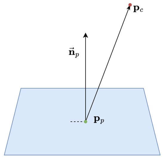
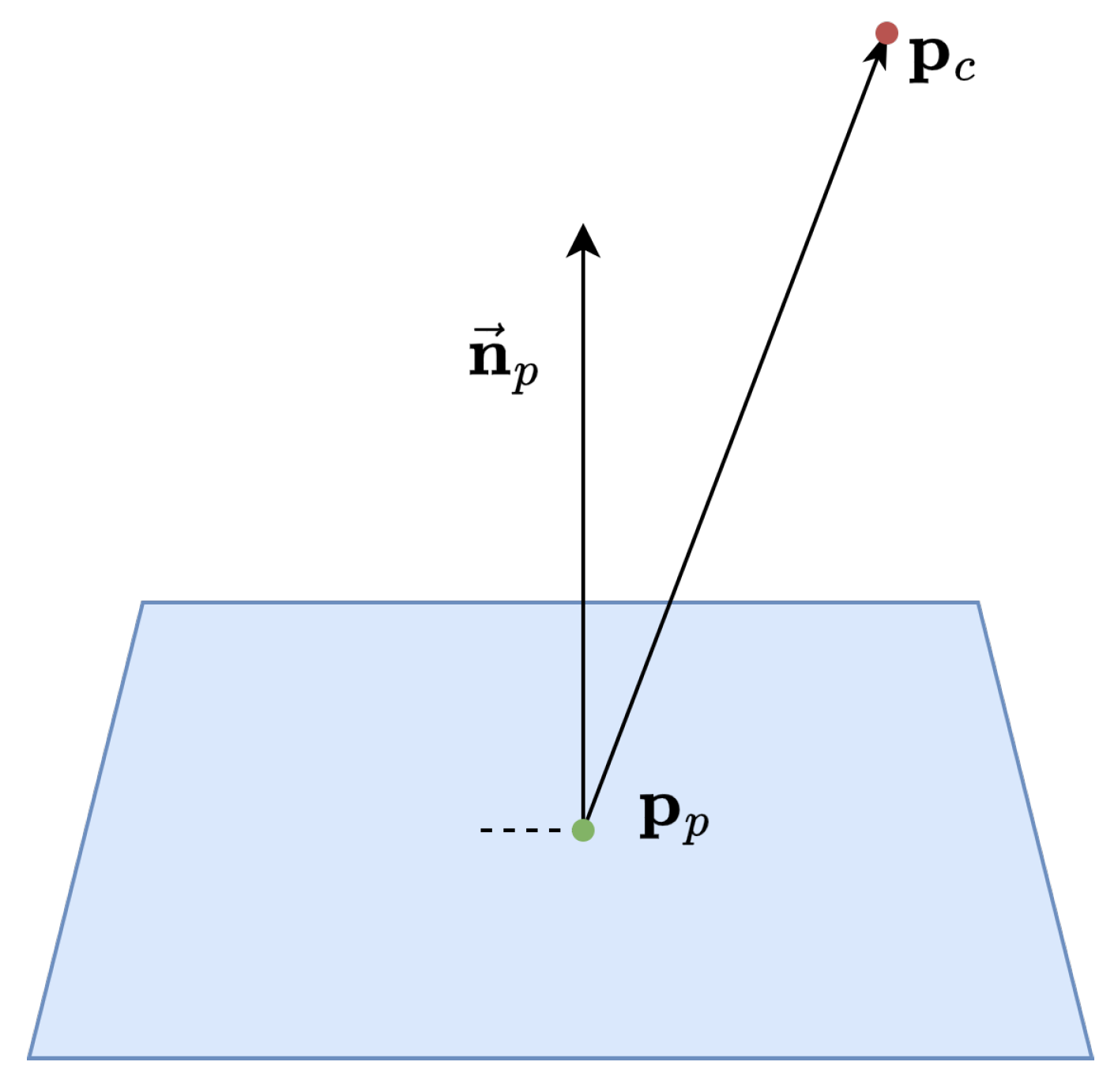
Our camera view planning algorithm determines the best camera pose to observe a certain small patch of skin (defined by the centroid () and the normal () and shown in Figure 1). The camera is defined as a rigid body with a pose () that can described by Special Euclidean Group SE(3):
Figure 1.
Representation of the patch defined by its centroid () and its normal vector (), as well as the camera view position () for the observation of the patch.
The algorithm considers five main objectives:
- 1.
- The resolution (metres per pixel) of the image taken with the camera at the specified position;
- 2.
- The orthogonality of the camera’s observation angle with respect to ;
- 3.
- The projection of the skin lesion’s 3D coordinate () onto the camera’s image space;
- 4.
- The safe distance of the end effector (where the camera is located) from any object present inside the environment, including the patient (defined by the set of obstacles () on the surface of the collision mesh ());
- 5.
- The occlusion of the patch as viewed from the camera, caused by any arbitrary obstacle located between the camera and the patch ().
The fourth and fifth objectives are of the utmost importance and are two out of the five that have to be respected. They prevent the process from generating an image without a view of the patch and from causing both damage to the camera system and harm to the patient currently being scanned.
3.2. Resolution
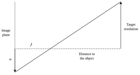
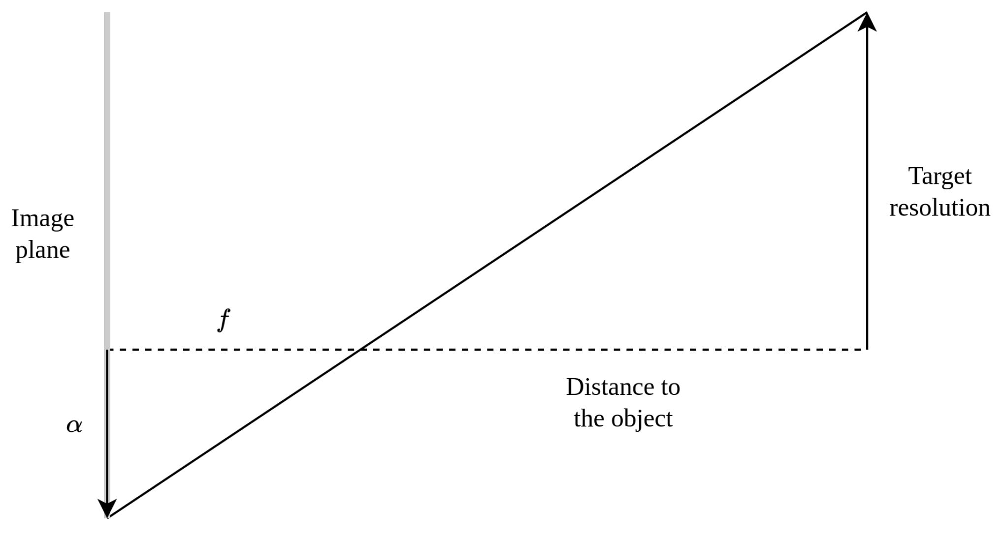
The resolution of the output image is controlled by the distance between and . Using the pinhole camera model (Figure 2), we can define a relationship between the camera’s intrinsic parameters, the distance to the patch and the desired resolution.
Figure 2.
Pinhole camera model representation with focal length in metres (f), the pixel size of the sensor in metres (), the distance to the object in metres and target resolution in metres.
The resolution can be calculated via
where is the resolution in metres per pixel, is the pixel size of the sensor in metres and is the focal length in metres.
The same equation can be rewritten to calculate the Euclidean distance () from to that will produce the best resolution ():
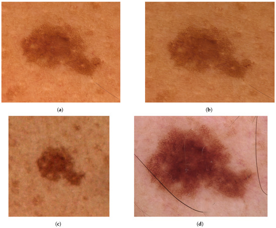
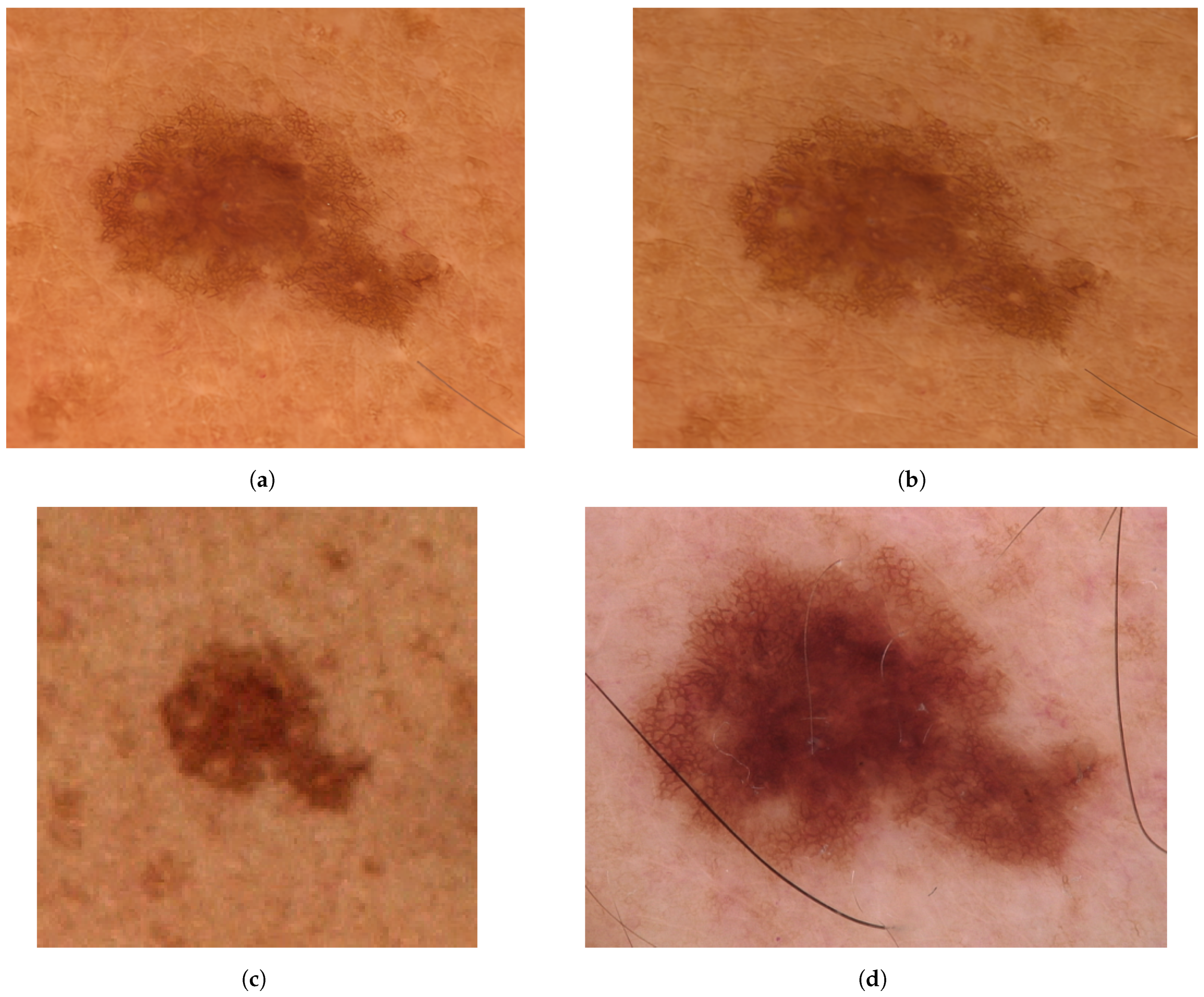
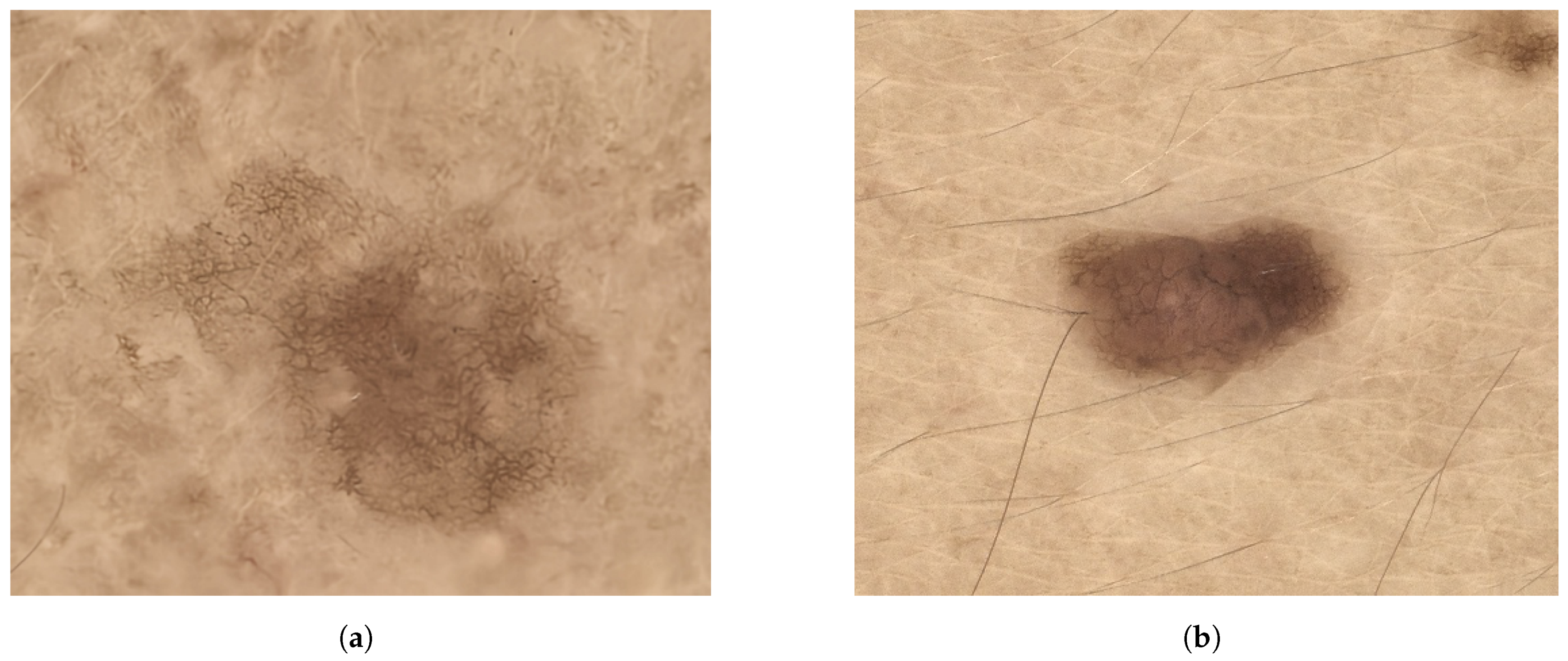
Figure 3a,b show the same mole captured by the dermatoscopic camera at two different distances (35 cm and 40 cm), producing images with resolutions of 16 /px and 19 /px, respectively. The left image was captured from the ideal distance, providing a better resolution for the mole. The right one was captured 5 cm from the ideal distance, with a slightly worse resolution. Figure 3c,d display the same mole captured by a VECTRA system (state-of-the-art full-body imaging scanner) and a handheld dermoscope, respectively, with approximate resolutions of 100 /px and 10 /px. A higher resolution image provides the means to visualise features of pigmented melanocytic neoplasms, which are fundamental for doctors to be able to diagnose different types of melanomas. These features are impossible to discern from lower resolution images, making higher resolution images critical for accurate diagnosis. In fact, dermatologists rely on five primary dermoscopic features for clinical diagnosis (listed in Figure 3). While images captured with our method and with a handheld dermoscope retain all five features, commercial full-body scanners (e.g., VECTRA) are limited to resolving only one (#5). In Figure 3a,b, all five features are visible; however, and are sharper and easier to distinguish in the higher resolution image.
Figure 3.
Dermoscopic images captured at (a) 35 with 16 /px resolution and (b) 40 with 19 /px resolution using our method. The same mole captured (c) with the VECTRA at a resolution of 100 /px and (d) with a handheld dermoscope at a resolution of 10 /px. Visible dermoscopic features include the following: (1) a predominantly reticular pattern: a pigment network is present and more evident at the periphery; (2) and irregular/atypical network: the network shows variable line thickness and mesh size, with areas where it looks broader and less uniform; (3) central structureless hyperpigmentation: a darker brown central homogeneous/blotchy area (confluent pigmentation); (4) a focal hypopigmented/structureless areas: at least one pale/whitish, roundish area within the lesion, plus a few smaller, lighter, structureless spots; (5) asymmetry in the overall contour and pigmentation distribution.
3.3. Orthogonality
The alignment of the camera position () with the normal to the patch () enforces an orthogonal viewing direction of the camera with respect to the plane of the patch. This orthogonality is an important factor to consider for the resulting quality of the image.
As the observation angle becomes more slanted, it gradually changes the shape of the skin lesion as seen from the camera. In addition, if the camera has a short depth of field (which is especially true for dermatoscopic cameras using liquid lenses), some pixels will appear in focus, while others will not. A more slanted observation angle causes the difference between the minimum and maximum distance from the camera to the object points to increase.
The orthogonality can be modelled by a function that calculates the angle between the camera viewing direction, defined by , and the normal to the patch (). When the camera viewing direction and the plane of the patch are perfectly orthogonal, the angle is zero, and there is no perspective distortion of the patch on the image. As the angle approaches 90 degrees, the viewing direction and the plane become parallel, causing the distortion to increase until the patch is no longer visible inside the image.
3.4. Visibility
The visibility (v) of the patch can be defined in different manners. In the simplest solution, the centroid of the patch () can be projected onto the camera’s image plane in pixel coordinates, and if the point lies within the image boundaries, the point will be visible:
where is the transformation matrix from the world frame to the camera frame, is the camera’s intrinsic matrix, is the projection of onto the image plane and is the subset of points that lie within the image.
However, this function is non-differentiable, that is, it is not the optimal representation in an optimisation problem where the objective is to use the function’s gradients to guide the minimisation procedure.
A better representation would be a smooth symmetric function that gradually approaches zero as the projection of on the image plane goes out of bounds. To do this, we reproject the point onto the image plane and compute the distance from the reprojection point to the camera’s optical centre.
3.5. Safe Distance
The safe distance defines a minimum distance from any object within the environment to stop the camera from getting too close (while seeking a better position to observe the patch) and potentially hitting an object or harming the patient.
The camera sits inside the cobot end effector. As such, the view planning algorithm must consider the entire geometry of the end effector when computing the safe distance to the obstacles inside the environment.
The equation for safety is defined for a specific point of the end-effector structure (the camera position). We extended this computation for a selected number of points () defined to form a security cage around the end effector. In this manner, the optimisation is aware of potential collisions with the end-effector structure when translating and rotating the camera.
3.6. Occlusion
The occlusion parameter defines the visibility of the patch from the current camera pose. In contrast with Section 3.4, it does not define the visibility of the patch as a function of the reprojection of onto the image plane or whether it falls within the image bounds. Instead, the occlusion also depends on the obstacles inside the environment. If an obstacle lies along the ray connecting the camera’s optical centre to the patch, then the patch is said to be “occluded”, i.e., it cannot be seen within the captured image.
3.7. Problem Description
The optimisation attempts to find the best camera pose () that minimises the cost function (f) defined below. is represented by the SE(3) group of rigid body motions. However, the problem is not modelled directly on the SE(3) manifold but, rather, on the tangent space of the manifold (). The derivatives could not be computed for our problem; therefore, we required numerical differentiation to solve it. However, the local solver we were utilising, i.e., the Ceres solver [24], only provides support for manifold optimisation for problems whose derivatives can be defined either analytically or using automatic differentiation. For this reason, we elected to work on the tangent space of the SE(3) manifold to leverage the SE(3) manifold’s properties and to allow the numerical solver to move in linear space ().
When using solvers with built-in support for manifold optimisation, the user needs to only worry about modelling the problem on the manifold space. The solvers already integrate Exp and Log operators and their derivatives, which they use to perform the conversion between tangent and manifold spaces and to propagate the error from the manifold to the tangent space. Our problem, however, is defined numerically and, thus, requires a small modification to the cost function.
The state is defined as a vector in the tangent space [25]:
where , is the translation component of (where is a different entity from the translation () in Equation (1)) and is the rotation component of .
Therefore, to compute the camera pose, the state vector is used to apply a perturbation in the tangent space (), then retracted into the manifold space (SE(3)). Together, the two operations define the right-plus operator (right-⊕) [25]:
The cost function (f) is defined as follows:
where and is the safe distance. Residual functions for resolution (), orthogonality () and reprojection (), which define the loss function () (, and ) are defined in Section 3.8, Section 3.9 and Section 3.10 below. Safety and occlusion functions ( and ), as defined in Section 3.11 and Section 3.12 below, instead define areas of high loss that are employed to steer the optimisation towards valid areas (away from the patient and where the patch is visible from within the image). All the residual terms in are normalised to unit scale. Therefore, when the safety and visibility conditions are violated, they are penalised to the maximum admissible error (i.e., 1), ensuring that constraint violations drive the optimisation away from those regions of the search space. This can be observed in , where the vector represents a column vector with a length of four.
3.8. Resolution Residual
The resolution residual function is given by
where is the residual function with a six-dimensional input (the tangent vector () of the SE(3) manifold). This function models the quality of the image in terms of resolution. It computes the distance between and and compares it against the ideal distance (). The value of is defined as the distance from the patch that gives the ideal image resolution and, thus, the best image quality.
As one moves away from the ideal distance from the patch, the error increases.
The maximum distance () describes the maximum difference of the dermoscopy resolution relative to the ideal resolution. A smaller difference means the distance from the patch will not vary significantly from the ideal distance (); consequently, this also implies that the output dermoscopy resolution will not experience a noticeable degradation from the ideal resolution, i.e., (Equation (3)). The parameter is used to normalise the residue to improve the numerical stability of the cost function during the optimisation process.
3.9. Orthogonality Residual
The orthogonality residual function is defined as
where is the residual function with a six-dimensional input (the tangent vector () of the SE(3) manifold), which calculates the error based on the angle (Equation (4)). It models the orthogonality of the patch to be observed as the angle of incidence () of the camera’s view direction vector (defined by ) on the plane of the patch (defined by the normal vector, i.e., ).
The maximum angle from the patch is defined as . The residual is at its minimum at zero, where the error is the smallest (when the camera’s image plane lies parallel to the plane of the patch) and increases until it reaches maximum error at . Any angle above prevents the patch from being observable. However, the maximum angle can be decreased further to enforce a range of values wherein the patch has minimal distortion. Like in Section 10, the parameter normalises the cost function and adds numerical stability to the problem.
3.10. Visibility Residual
The visibility residual function is given by
where is the residual function, which calculates the error based on the distance of the reprojected point from the centre of the image (in both the x and y directions). It models the visibility of the patch to be observed as the distance from the reprojected patch centroid () with respect to the camera’s optical centre .
The maximum reprojection distances from the camera’s optical centre are defined as and . The residue is at its minimum at zero, where the error is the smallest (when the reprojection of the patch centroid () coincides with the centre of the camera’s image plane), and increases until it reaches its maximum error at and .
3.11. Safety Function
The safety function is evaluated between every obstacle () inside the environment and every risk point () on the end effector’s structure. The obstacles include both the patient’s surface and the bed on which the patient is lying.
The safety function is given by
where is a function that computes the minimum distance between each obstacle () inside the environment and each risk point () on the end effector’s structure. Each pair evaluates a different distance, providing a vector of distances from which the minimum is extracted to help the solver steer the end effector away from possible collisions. As described in Section 3.7, the output of is compared with the safety distance (), and if found to be smaller, it increases the value of the residues of the loss function ().
Thus, the value of the safety function helps create a security bubble around each obstacle to prevent the cobot’s end effector from getting too close and potentially colliding with it.
3.12. Occlusion Function
The occlusion function is evaluated for every obstacle () inside the environment, where includes both the patient and the scanner’s bed.
The occlusion function is given by
where is a function that returns a boolean value (true or false) for occlusion. It defines a ray () with an origin at the camera’s optical centre () and a direction vector pointing towards the patch (). The ray is then cast, and if the hit distance () is smaller than the distance from the camera to the patch, the patch is considered occluded by an obstacle.
The value of the occlusion function helps the camera pose steer away from areas where other obstacles may be located in the viewing direction, ensuring that the patch remains visible in the captured image.
3.12.1. Initialisation
One of the main limitations of local optimisers such as Ceres [24] when solving nonconvex optimisation problems is their sensitivity to the initial point. They are designed to find a locally optimal solution; however they do not guarantee global optimality, especially with nonconvex problems (like ours).
For this reason, we developed a discrete sampling algorithm to find the best feasible initial points inside our environment, i.e., safe () and visible () points with the lowest resolution () and orthogonality () residues. Due to the nature of our problem, a conical sampling approach was chosen. The maximum focal distance error ( in Equation (10)) defines the height of the cone, and the maximum incidence angle error ( in Equation (12)) defines the half-aperture angle of the cone. Positions are sampled inside a cone that defines the bounds of the problem, and using the obstacles inside the environment, the points are selected or ignored based on the safe distance ( in Equation (14)) and occlusion.
The algorithm first samples points inside a cone with respect to a local origin using the problem’s predefined hyperparameters (, ). Afterwards, based on the patch’s normal and centroid, these points are first translated and rotated with respect to the new reference frame (the patch, where the z axis is aligned with the normal); then, each individual point is evaluated against the obstacles inside the environment to determine the occlusion and safety parameters.
3.12.2. Planning Algorithm
Using the strategies described above, the implementation of our algorithm can be split into four main sections (Algorithm 1):
- 1.
- Validity check of ideal camera pose.
- 2.
- Calculation of the initial camera poses (Section 3.12.1).
- 3.
- Optimisation of the camera poses.
- 4.
- Selection of the best camera pose.
| Algorithm 1 Finds the optimal camera view position |
|
The first step involves the following equation:
Equation (17) describes the ideal camera view position with no constraints, i.e., with no obstacles in the environment, and, thus, with complete freedom of movement. This position is at exactly the ideal distance from the patch to capture the image at the correct resolution and along the vector orthogonal to the plane of the patch, preventing any warping deformation of the features of the patch in the output dermatoscopic image (caused by a slanted angle of observation). The z axis of rotation will point directly to the patch (). The remaining axes (x and y) are chosen based on the safety function (g, Equation (14)), as certain configurations may cause a collision between the end effector and the obstacles.
If the patch is not occluded by any of the obstacles and if the points that were found are all farther away from the ideal camera position (, Equation (17)) and the end effector’s risk points () than a distance equal to or greater than the safe distance (), then the ideal camera pose will be selected as the final camera view position. Since there is no occlusion and no risk of collision, optimisation will not be required.
The second step is the initialisation of the valid camera poses (described in Section 3.12.1) for the optimisation.
The third step is the optimisation. The valid initial camera poses () will be utilised as starting points for the optimisation. Each of the initial points will be employed in a parallel optimisation run.
The fourth and final step is camera pose selection. If all of the optimised poses fail to meet the conditions (either outside the distance bounds, outside the angle bounds, outside of the camera’s FOV, too close to the obstacles or occluded), then the optimisation is deemed unsuccessful. If there is more than one valid camera pose, the one with the smallest objective value (f, Equation (8)) is chosen as the optimal camera pose.
4. Results and Discussion
4.1. Description of System
The planner was written in C++, and the Ceres Solver (version 2.2) [24] was employed as a local optimiser for the problem. The residual functions were modelled as a non-linear least-squares problem using Ceres, and the optimisation was solved numerically using the central differences method.
For the experiments, the system that was employed was a Dell Inspiron laptop from 2015 running Ubuntu 20.04 with 16GB of RAM, an Intel Core i7-8565U processor (4.6 GHz) and an NVIDIA GeForce MX150 graphics card.
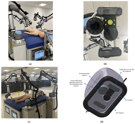
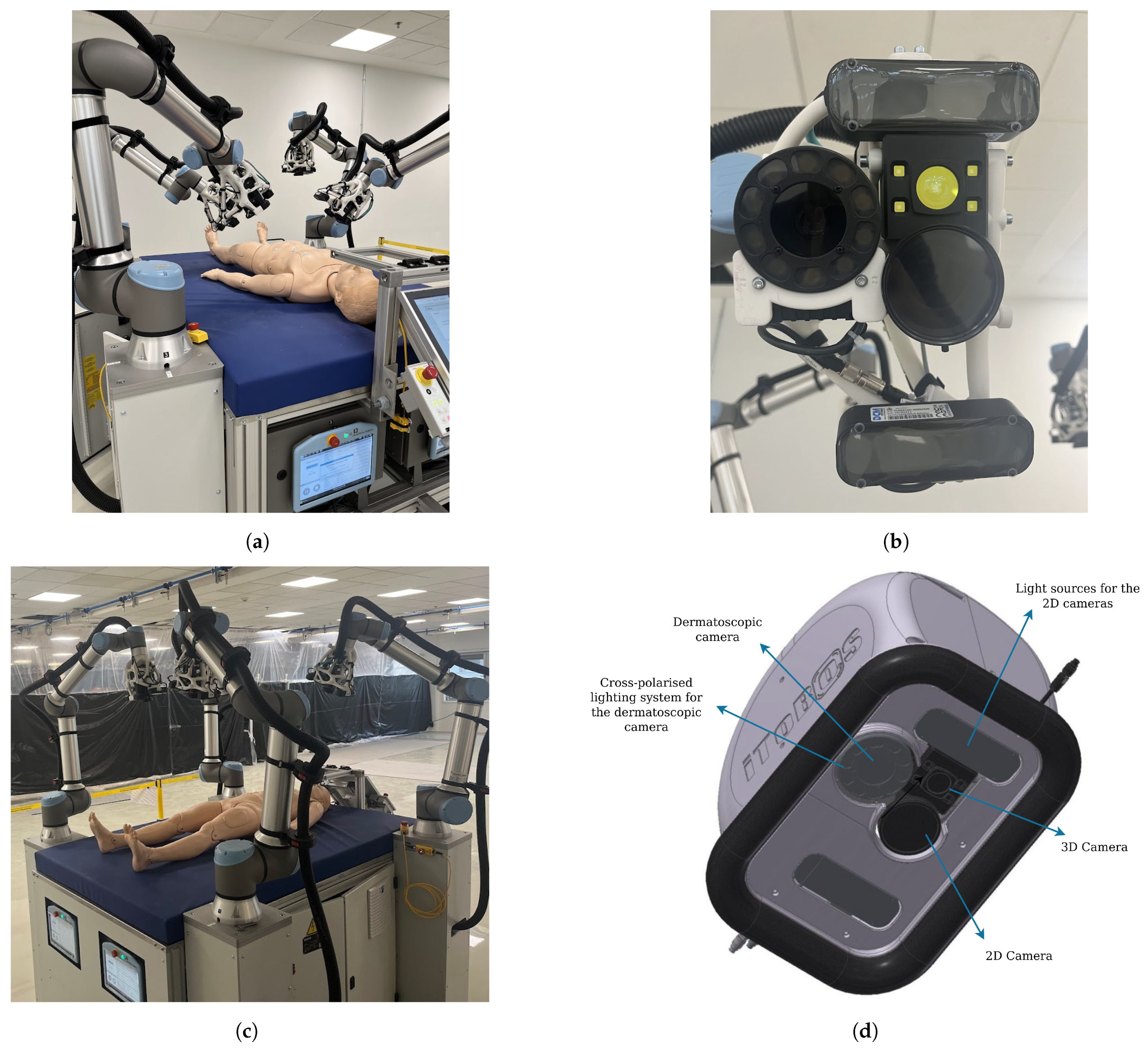
The full scanner system can be observed in Figure 4a,c. Other than the cobots, which are fixed to the ground on separate platforms, the scanner also includes a bed with a mattress and the main computer.
Figure 4.
(a,b) The scanner with a mannequin on the mattress. The scanner is composed of four cobots, each possessing an end effector holding together the three cameras. Behind the mannequin’s head sits the touch panel that controls the scanner. (c) Photos of the end effector without the protective structure showing only the cameras. (d) CAD drawing of the bottom view of the end effector. Three cameras are located inside the end effector: a 2D camera, 3D camera and dermatoscopic camera. The 2D camera is the circular camera in the centre, the 3D camera is the square-shaped camera next to it, and the dermatoscopic camera is the larger circular camera on the side of the end effector.
The three different cameras on each end effector are enclosed in a cage-like structure to protect the internal electronics from damage if any collision were to occur between the different cobots. The cobots’ workspaces overlap with each other; therefore, there is a risk of collision that needs to be managed. In Figure 4b,d, the three cameras can be observed in the central section, with two on top and one right below. The 3D camera corresponds to the square-shaped one in the top-left, the 2D camera corresponds to the circular one to the right of the 3D camera, and the dermatoscopic camera corresponds to the large circular one on the bottom.
4.2. 3D Patient Scans
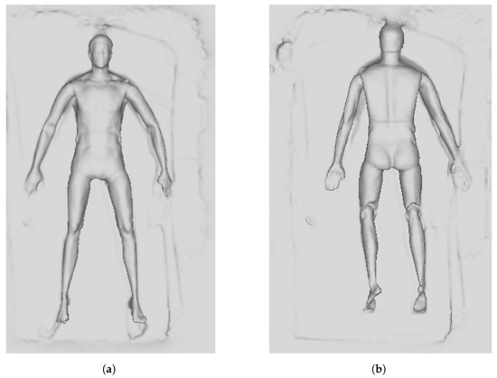
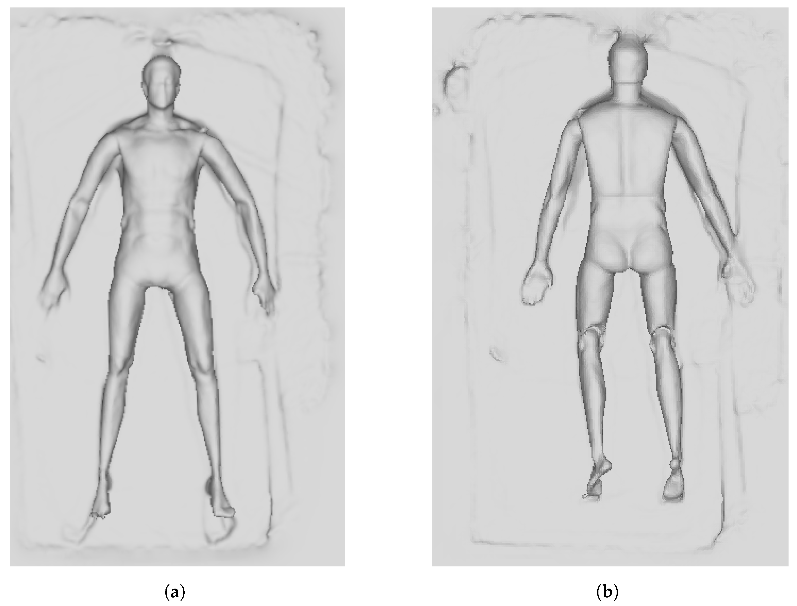
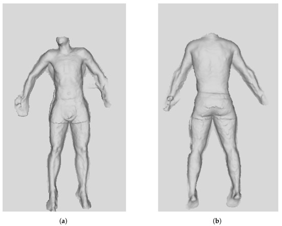
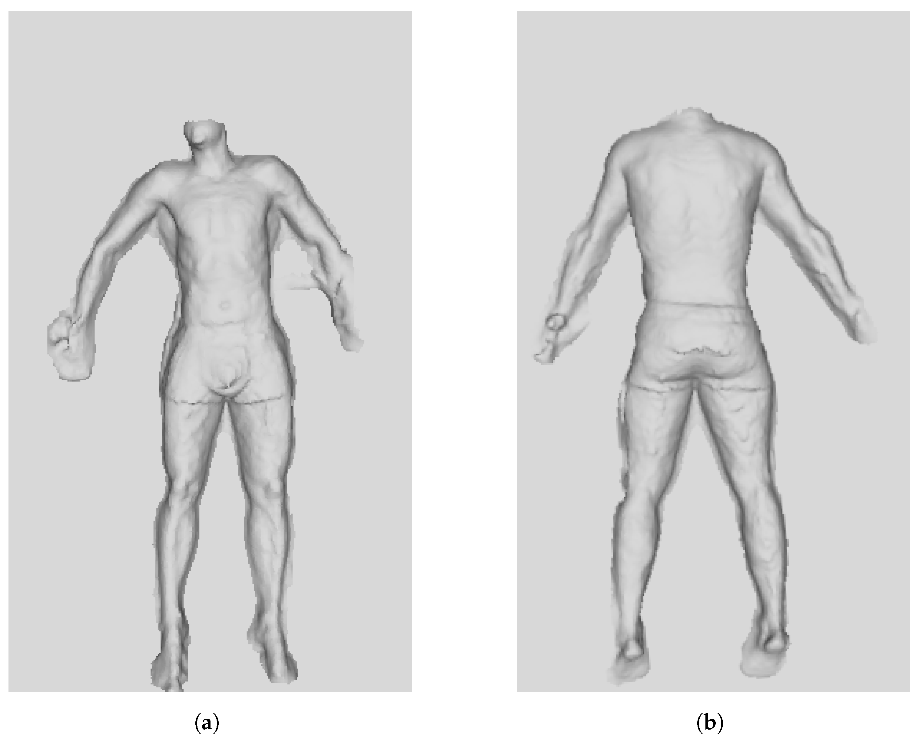
The reconstructed 3D mesh containing the points from the patient and the patient’s bed was generated by making use of the 2D and 3D cameras. The 3D reconstructions were obtained using structure from motion applied to multi-view RGB and depth images, followed by Poisson surface reconstruction to generate watertight meshes [26]. Finally, surface normals were estimated using local neighbourhood fitting. Examples of a 3D reconstruction of a mannequin and a real patient lying down on both sides are shown in Figure 5 and Figure 6.
Figure 5.
Reconstructed mesh of a mannequin placed on a mattress in supine (a) and prone (b) positions.
Figure 6.
Reconstructed mesh of a patient placed on a mattress in supine (a) and prone (b) positions.
4.3. Experimental Setup
The optimisation tests were run on the scanner with both a mannequin and real patients placed on it.
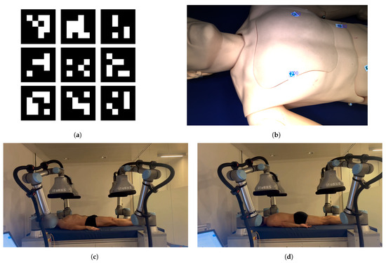
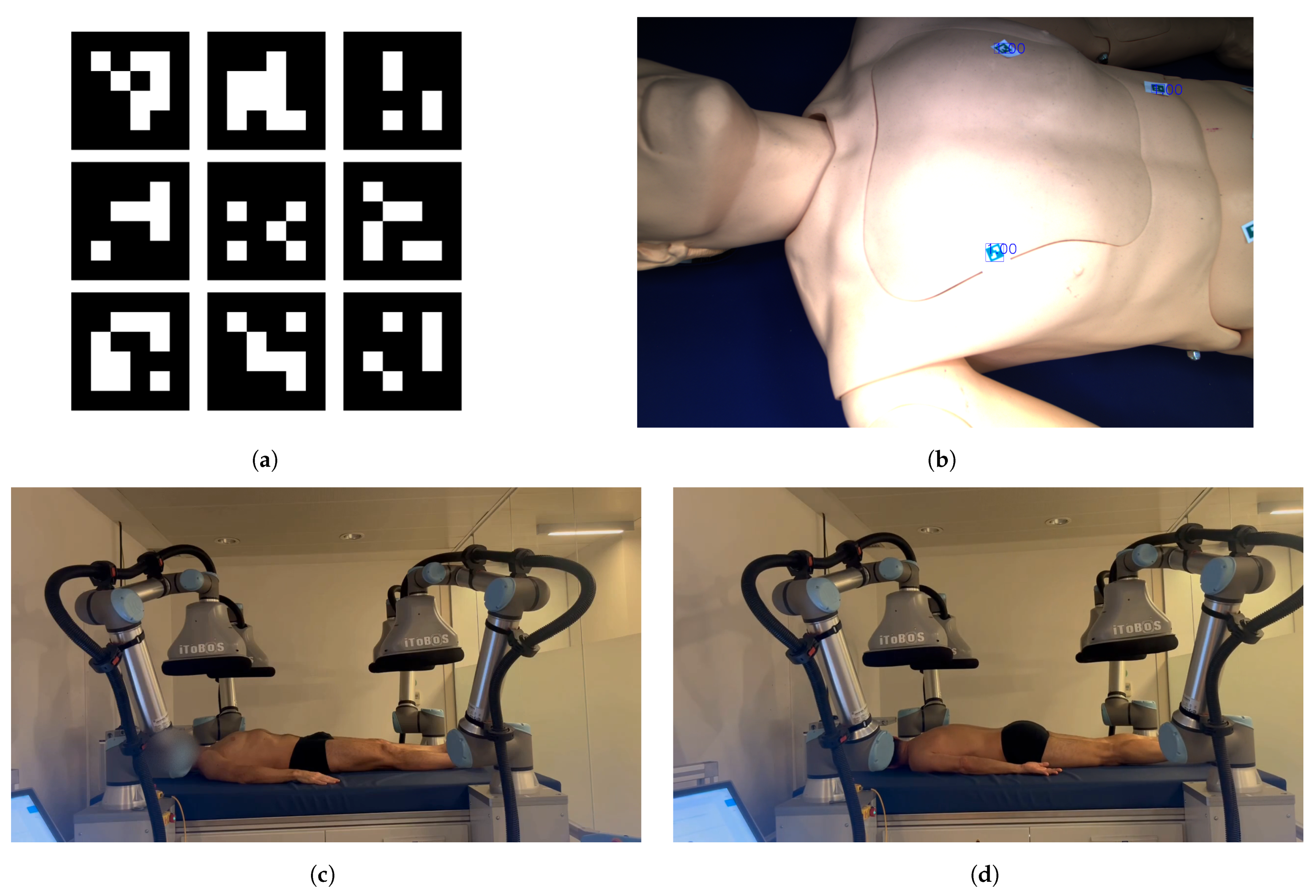
In order to perform tests on patches of skin, it is necessary to obtain their position and surface normal. The mannequin does not possess skin lesions. Therefore, several ArUco markers [27] were placed on multiple places on the surface of the mannequin to act as artificial “patches”.
The mannequin with the ArUco markers was used to perform quantitative tests, as it allowed us to evaluate the final camera poses with ground-truth data. Real patients were used for qualitative tests. Tests with real patients entail a higher degree of uncertainty in the point cloud and in the reconstructed 3D mesh of the body but also permit us to determine the algorithm’s performance on a real-life test case. This, however, comes at the cost of a lack of ground-truth data (Figure 7c,d).
Figure 7.
(a) Examples of ArUco markers (not to scale) placed on the mannequin. (b) Image from the 2D camera on the robot end effector with ArUco detections on the mannequin. Experimental setup with a real patient in (c) supine and (d) prone positions.
The ArUco markers were generated from the ArUco dictionary named “DICT_4x4_50”. This dictionary is composed of 50 markers, each of which has a size of bits and a side length of 1 .
Figure 7a shows some samples of the markers that were placed on the mannequin. The markers were then detected during the scanning process (Figure 7b), and the position and normal were passed to the camera view planning algorithm. Once the output camera pose was sent to the scanner’s control algorithm and the image was acquired, the resulting image was assessed to determine whether the camera planner was able to correctly take a picture of the selected marker.
As described in Section 4.1, the experimental setup consists of four cobots placed on the corners of the patient’s bed. However, our proposed method does not require them; it can operate with a single robot executing the same view-planning and acquisition pipeline sequentially. Four collaborative robots were used in our prototype to reduce acquisition time by parallelizing viewpoint exploration and imaging, i.e., to improve throughput rather than to satisfy an algorithmic requirement.
The experiments involved both a mannequin and real patients. When performing the scan on the patients, we observed slight patient motion, which could have affected the precomputed 3D model and planned poses. However, robust motion compensation and tracking are outside the scope of this paper, which focuses on safety-enforcing and occlusion-aware view planning under the assumption of quasi-static geometry during a short acquisition window. In practice, the workflow included a straightforward safety fallback: either the patient or the technician could cancel the scan at any time (e.g., in case of discomfort or observable motion), after which the scan could be restarted.
4.4. Optimisation Tests
Three series of results will be presented in this section:
- 1.
- The workflow of the optimisation algorithm;
- 2.
- The trade-off between the cost function’s five objectives (described in Section 3.1) between the ideal and optimised camera poses;
- 3.
- The effect of the number of initialisation points on the speed and the accuracy of the optimisation.
Based on the end-effector structure shown in Figure 4d, five risk points () were chosen: the centre of the end effector and the four sides of the end effector, i.e., , , and (in centimetres), all computed with respect to the camera’s optical centre.
Our method solves a specific problem that existing literature has not yet addressed: maximizing the image quality of the features of a known surface patch while strictly enforcing safety and visibility constraints. Current state-of-the-art algorithms (e.g., NBV) focus on exploring unknown spaces or simply covering every part of a surface.
Since no current algorithm targets this specific objective, a direct comparison with the state of the art is not possible. The metrics used to evaluate exploration or simple coverage do not apply to our objective of achieving optimal image quality. Therefore, we demonstrate the effectiveness of our approach through its ability to solve this new problem directly rather than through benchmark comparisons with incompatible methods.
4.4.1. Visualisation of Optimisation Process
For the experimental results, the following hyperparameters were chosen: a safety distance () of 15 , an optimal resolution distance () of 25 , a maximum distance from optimal resolution () of 20 , a maximum incidence angle () of 45 and a maximum reprojection distance () of 20 .
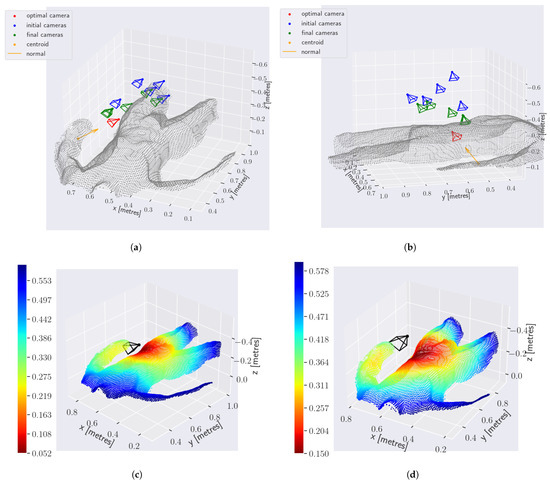
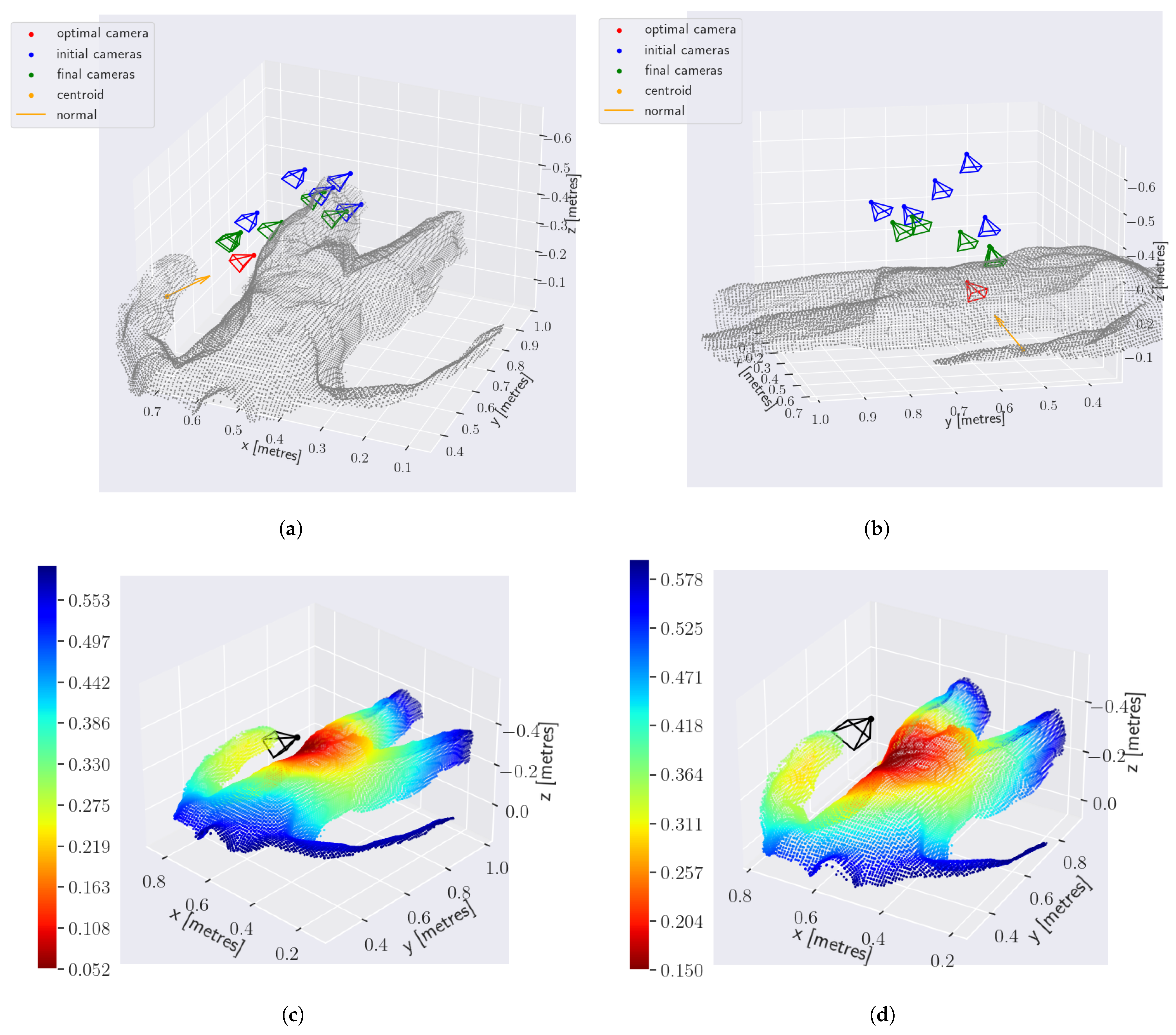
Figure 8 displays the camera optimisation of a single camera pose. Figure 8a,b show the input information available to the optimiser (the centroid and normal of the patch to take a picture of and the obstacles), and the initial and final camera poses. The two figures show the same information but from two different viewpoints. In this particular case, five initialisation points were chosen for the camera view planning algorithm. Figure 8c,d show the impact of the camera view planning algorithm. The ideal pose in terms of image quality is show in Figure 8c in black. It lies at a minimum distance of from the patient, which is far below the 15 minimum safe distance, as indicated by the red obstacle points in the vicinity of the camera. Once the optimisation is over (Figure 8d), the same points now lie at a distance of 15 (which is the safe distance) above the camera. This demonstrates the safety aspect of our camera view planning algorithm. Initially, the ideal camera pose was orthogonal to the normal of the patch, and it was located at exactly the optimal resolution distance from centroid of the patch ( 25 ). Upon termination of the optimisation, the optimised camera pose (and the entire end-effector structure) lies at a distance of ( from the optimal distance), at an angle of 21.2° degrees from the normal and at a reprojection distance of ( , ) from the camera’s optical centre. Thus, the view planner sacrificed the optimality of the camera pose to ensure the safety of the patient and of the scanner. Moreover, the final camera pose is free of occlusions, and the patch is clearly visible inside the image, as the reprojection error increased only very slightly from zero (less than 1 ).
Figure 8.
(a,b) 3D plots displaying the ideal (in red), initial (in blue) and optimised (in green) camera poses, as well as the centroid and normal (in orange) belonging to the patch to be observed and the nearby points that represent the obstacles to stay away from (in grey). 3D plots displaying the ideal (c) and optimised (d) camera poses (in black) and the obstacle points, with a colour map that displays each obstacle point’s distance from the camera positions (in metres), with red being the closest distance and blue the farthest. All the plots show the same scene from four different view points.
4.4.2. Trade-Off Between Patient Safety and Image Quality
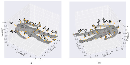
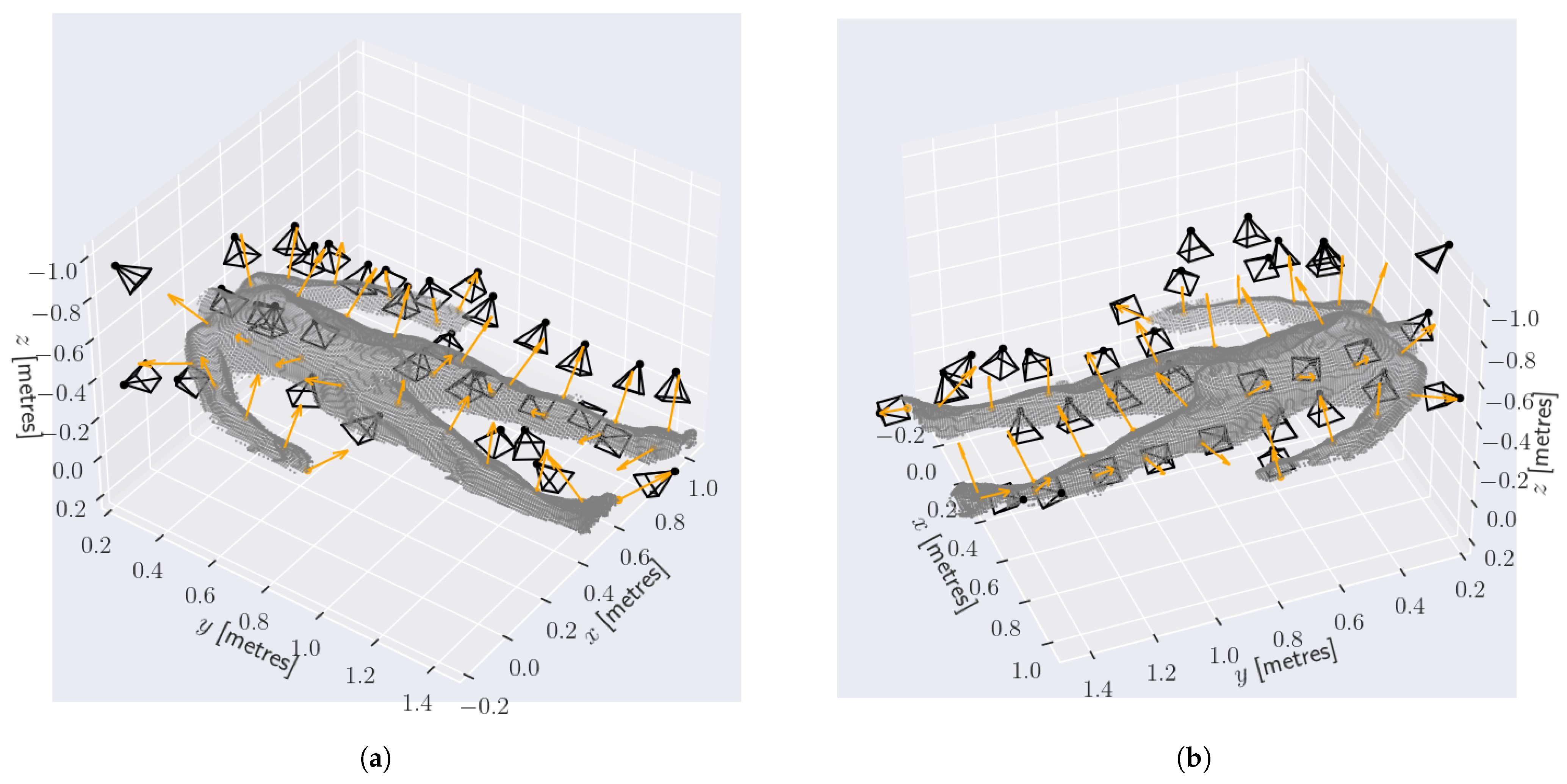
Figure 9 and Figure 10 show qualitative results of optimisation tests that were run on the model placed in a prone position. In order to avoid bias from a particular body area, the tests were carried out with points from all over the surface of the patient’s skin.
Figure 9.
Centroid and normals of the patches of skin of a patient (orange) and the corresponding camera poses computed by the camera view planning algorithm (black). (a,b) Two view points of the same scene.
Figure 10.
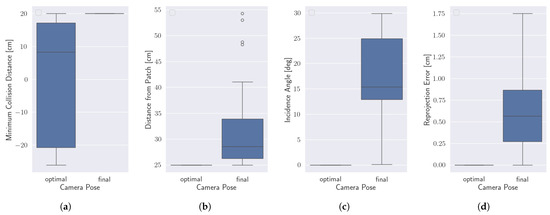
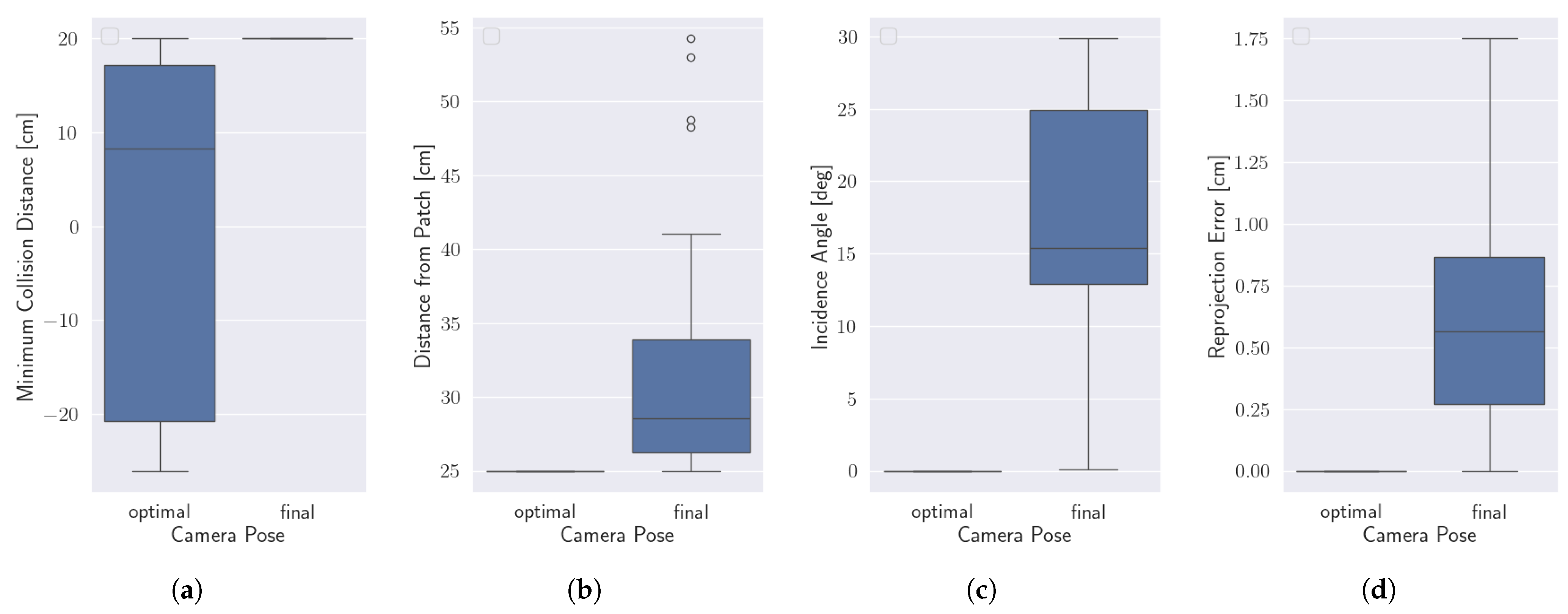
Box plots showing, for each patch, (a) the minimum distance from the patient to the end effector, (b) the distance from the patch to the camera position, (c) the angle of incidence on the patch of the camera’s view direction, and (d) the distance from the camera’s principal point to the reprojected patch in normalised image coordinates for both the ideal (left) and optimised (right) camera poses. The negative values for the distances in (a) signify that the cobot end effector is inside the patient mesh.
Firstly, the point cloud of the 3D reconstruction belonging to the model was divided into 33 quadrants (each with dimensions of 23 × 18 cm), and afterwards, the centroid and the normal of the points in each quadrant was calculated. Usually, centroids are computed via an average of the enclosed points. However, since each quadrant incorporated large areas of the body, several centroid quadrants ended up below the surface of the skin, especially on the sides of the patient’s body (or located on curved surfaces, e.g., the legs). To avoid having to calculate the best camera position for an area “inside” the patient, each centroid was re-calculated by taking the projection of all the points inside the voxel on the normal vector and choosing the point with the minimum projection distance.
where is the set of points from the obstacle point cloud () that falls inside quadrant i, is the average of the points inside and is the normal computed from the points inside .
Thus, camera view planning was run for every voxel using the newly calculated centroids and the original normals. The optimisation was run with a safe distance of 20 and a resolution distance of of 25 . The maximum distance from the optimal resolution distance () was set to 30 , the maximum incidence angle to 60 degrees and the maximum reprojection distance from the camera’s optical centre to 20 .
The plot in Figure 9 shows the selected centroids and normals for the optimisation on the surface of the patient. For each camera view-planning procedure (for each voxel and for each configuration) and for both the ideal camera position (Equation (17)) and the optimised camera position (the output of the camera view planning), four measurements were extracted (Figure 10):
The plots in Figure 10 show the distribution of these four measurements for both the ideal camera position (left) and the optimised camera position (right). The centre line of each “box” describes the median; the upper and lower limits of the “box” describe the 25-th and 75-th percentiles; the upper and lower fences represent values smaller and bigger than the 25-th and 75-th percentiles by an amount equal to 1.5 times the difference between the 1st and 3rd quartiles, respectively; and the scattered points represent the outliers [28].
The difference in the median values and in the distribution of the values between the ideal and optimised camera positions describes the trade-off that is generated by the camera view planner. Initially, the camera pose is at the perfect resolution distance of 25 , in line with the normal vector of the patch (incidence angle of 0 degrees) and with the patch centred at the origin of the image, as observable on the left-hand side inside Figure 10b–d. However, in Figure 10a, the end effectors at the ideal camera poses are closer than the safe distances. The negative distance values signify that the end effector is inside the patient mesh. The minimum distances to the environmental obstacles vary from safe distances of 20 to collision areas inside the patient, with a median value of around 9 , thereby generating the majority of camera poses with a high risk of collision. The camera view planner attempts to reduce this risk by pushing the camera pose towards the range of the safe distances (as shown on Figure 10a). This comes at the cost of the resolution distance and the incidence angles, as well as, to a lesser extent, the reprojection error. As observable from Figure 10b–d, the angles now vary from 0.1 to 29.9 degrees, the distances from about 0 to above the ideal resolution distance and the reprojection of the patch onto the image from about 0 to from the image’s principal point. However, the median values sit at , 15.4 and , showing how the camera view planning algorithm is able to find a pose that ensures patient safety but without excessively reducing the image quality.
4.4.3. Number of Initialisation Points vs. Execution Speed
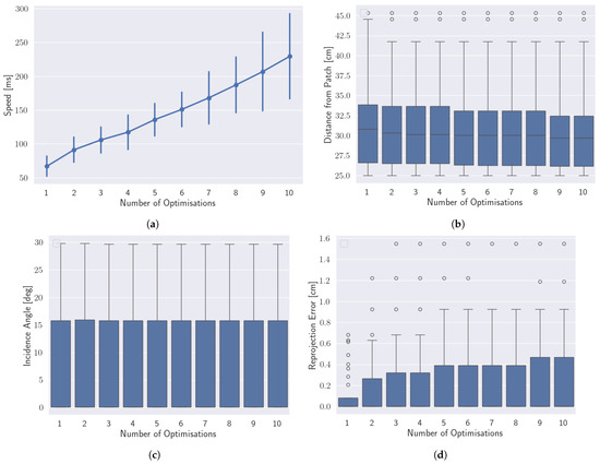
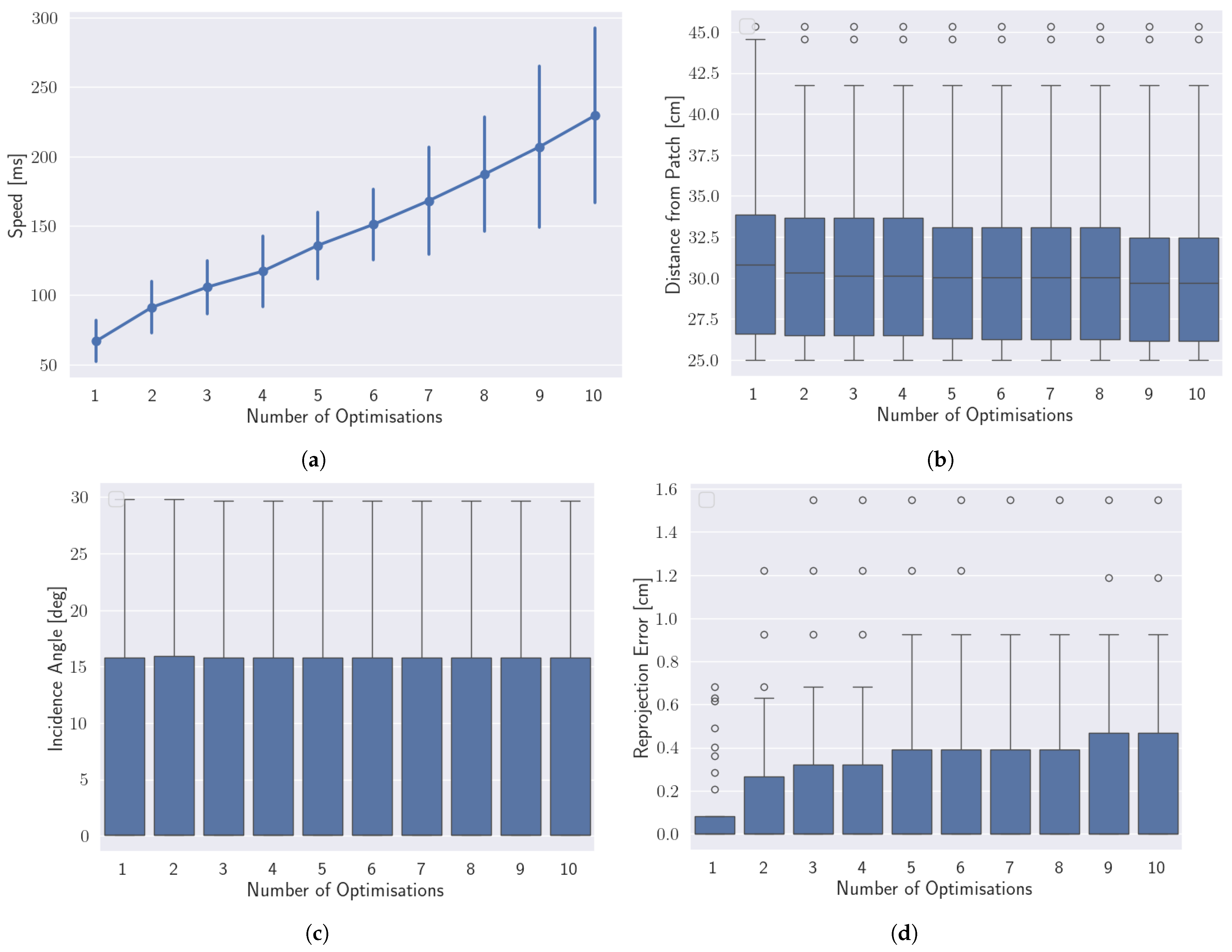
As previously mentioned, the bottleneck of the camera view planning algorithm is the number of initialisation points and, thus, the number of simultaneous optimisation procedures. The search space is complex; therefore, the local optimiser could run into local minima. A higher number of optimisations, each run from a different initialisation point, might help find the best camera pose out of all the local minima. We designed a test to show the effect of a higher number of initialisation points on the output and on the speed of the camera view planner while trying to observe the same patches of skin. We employed the same patches from the previous test to calculate the optimal camera poses. Afterwards, the same optimisation procedure was repeated with a different number of initialisation points, ranging from 1 to 10. The values of the hyperparameters remained the same as the ones from the previous test.
Figure 11a shows the speed of the entire camera view-planning procedure for different numbers of initialisation points. The error bars show the standard deviation of the execution speeds (at ) for each patch and for different numbers of initialisation points. The execution speeds increase linearly at a rate of about 18 per additional initialisation point, increasing from 67 for a single one up to 230 for 10.
Figure 11.
(a) Plot with error bars displaying the camera view planner’s execution time against different sampling numbers of initialisation points (and numbers of simultaneous optimisation procedures). Box plots showing, for each patch, (a) the minimum distance from the patient to the end effector, (b) the distance from the patch to the camera position, (c) the angle of incidence on the patch of the camera’s view direction, and (d) the distance from the camera’s principal point to the reprojected patch in normalised image coordinates (calculated with different numbers of initialisation points).
On the other hand, Figure 11b–d show the distance from the patch to the camera’s position, the angle of incidence on the patch of the camera’s view direction, and the distance from the camera’s principal point to the reprojected patch in normalised image coordinates, respectively, for different numbers of initialisation points. The distances and the angles do not improve with a higher number of initialisation points, keeping the same median values throughout.
This demonstrates that a higher number of initialisation points does not provide a significant advantage in terms of accuracy or precision. If we were to fit a line to the median values of each number of initialisation points, the slope would be close to zero. This is explainable by the fact that the initialisation procedure described in Section 3.12.1 already selects the best possible starting point inside the search space, always leading to an optimal camera pose. The remaining initialisations can be seen as almost redundant and can be avoided to maintain the same level of accuracy while speeding up the execution of the algorithm.
Our implementation uses a local optimiser that does not guarantee a global optimum. However, our formulation limits the practical impact of this limitation. The problem we are trying to solve is highly non-convex, but if we were not to consider the safety and occlusion components, the problem would become convex with a single well-defined global optimum. The non-convexity is introduced by these two terms. Therefore, there is only one camera pose that acquires the best possible image. What we are trying to find is the closest camera pose to the ideal one that enforces our safe distance and provides visibility (no occlusion). For this reason, our problem has an optimal solution in the local space around the ideal camera pose and can be simplified by using a combination of a targeted sampling algorithm plus a local solver, which is what was implemented. As presented in this section, through experimentation, we showed that running the optimization from multiple initialization points yields the same accuracy as using a single point selected by our sampling algorithm.
4.5. Dermoscopic Images
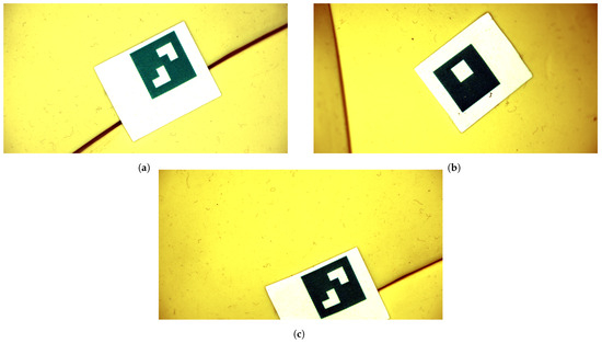
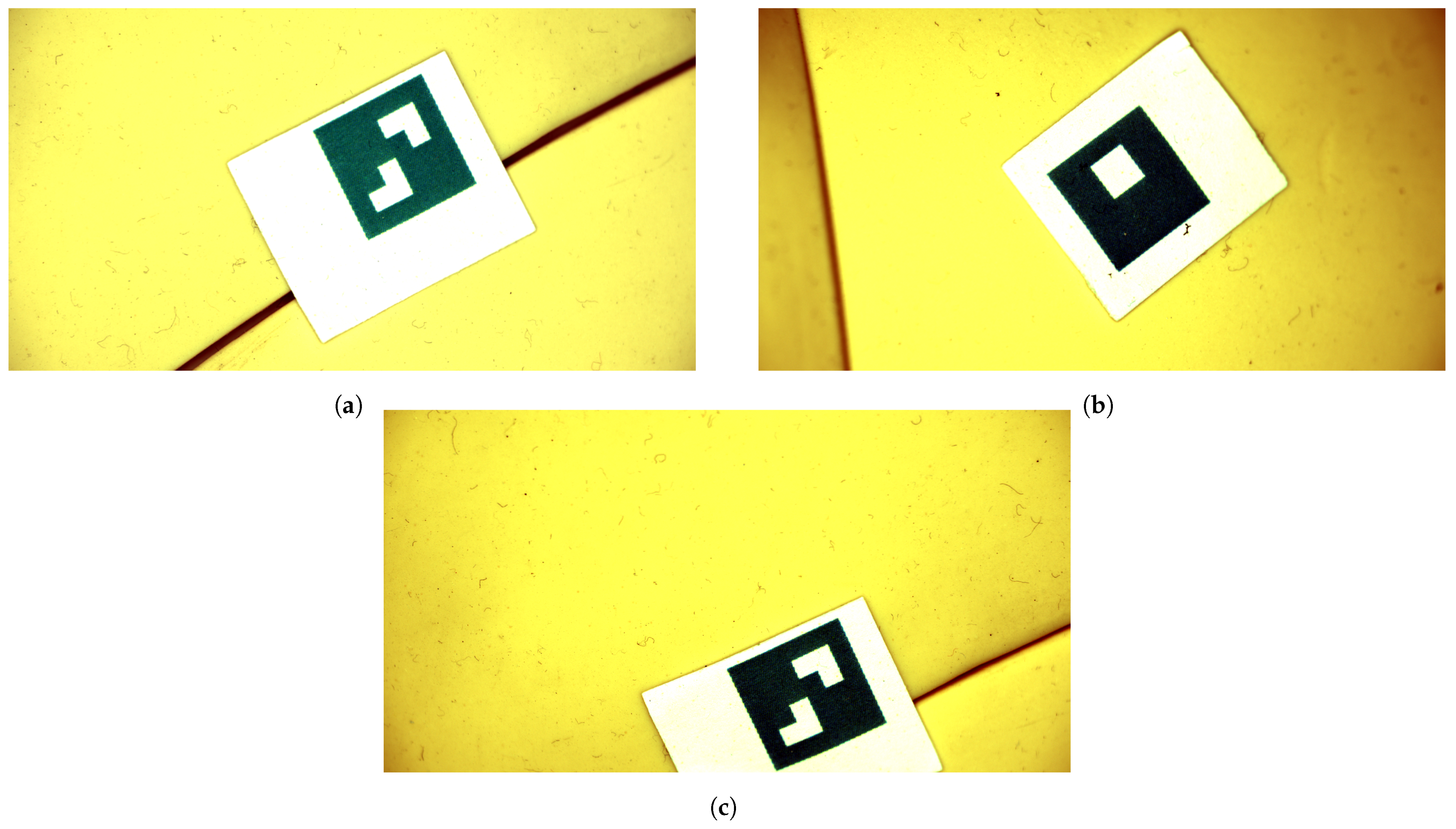
Figure 12 and Figure 13 display examples of dermoscopic images that were obtained after running camera view planning and moving the end effector to the calculated poses. The dermoscopic camera takes several images with varying focal distances; however, each focal distance possesses a very short depth of field (the portion of the image that is “in focus”, without any blur). Therefore, it is important to keep the camera within the range of distances covered by the focal lengths of the dermatoscopic camera, to minimise the angle of incidence with the patch and to centre the reprojection of the patch on the image, as it could cause only a part of the target (the ArUco marker in the image) to be “in focus” (Figure 12c).
Figure 12.
(a,b) Examples of images captured from the dermatoscopic camera from optimal camera poses calculated by the camera view planner and (c) from a sub-optimal camera pose (a slanted position), showing the reduced FOV when using a 100 lens.
Figure 13.
(a,b) Examples of dermoscopic images captured during the experiments with real patients.
5. Conclusions
In this work, we present a camera view planner designed exclusively for the observability of a small area on the surface of the skin. The planner takes into account the resolution of the image of the skin area, the angle of incidence of the camera’s view direction on the skin area, the location of the skin lesion within the image bounds, the distance of the end effector (where the camera is located) from any obstacle inside the environment and the occlusion of the skin area by any obstacles inside the environment. To the best of our knowledge, we are the first to develop a camera view planning algorithm for the observation of a specific area on the surface of an object (patient’s skin) and the first to develop a camera view planning algorithm for the observation of a skin lesion that aims to maximise the image quality and the safety of the patient (due to the proximity of the camera for such a task).
In our study, we used four manipulators, each equipped with a dermoscopic camera, placed around a medical bed. For the experiments, we employed both a mannequin with several ArUco markers, which acted as artificial “patches” (skin lesions), and real patients. The former allowed us to evaluate the results on a quantitative basis, while the latter introduced higher degrees of uncertainty in the generated 3D point cloud, helping us evaluate the effectiveness of our algorithm with real-life test cases.
We validated our algorithm by evaluating both image quality and patient safety. The camera pose for the best possible image quality can sometimes create discomfort for the patient due to proximity or, at other times, complete occlusion by other body parts. The camera view planner is able to maintain a safe distance from the patient in order to avoid any collision or patient discomfort by increasing the resolution distance and the angle of incidence but without significantly reducing the resultant image quality. It is also able to avoid areas where the skin lesion would be completely occluded. In addition, we also showed that for the optimisation to provide accurate results, it is not necessary to have a very high number of initialisation points to find the best local minima inside the complex search space. The algorithm is able to produce a close-to-optimal camera pose during the initialisation step, thereby removing the need for additional optimisation procedures. A higher number of optimisation procedures does not bring significant improvements in accuracy, demonstrating that the algorithm is able to produce the best possible result while performing at a real-time speed.
This paper demonstrates the technical feasibility of the algorithm as an alternative method to both total body photography and contact dermoscopy. It performs full-body imaging that is adaptable to the patient’s 3D geometry to capture moles from the best possible viewpoint within safe limits to avoid causing any discomfort to the patient and with a resolution that is comparable with a that of a handheld dermoscope, capturing the features that dermatologists use to determine the type of melanoma.
Supplementary Materials
The following supporting information can be downloaded at: https://www.mdpi.com/article/10.3390/technologies14040197/s1, Video S1: cameraviewplanning_video1.mp4.
Author Contributions
Conceptualization, V.F. and R.G.; methodology, V.F. and R.G.; software, V.F. and R.C.; validation, V.F. and R.C.; formal analysis, V.F.; investigation, V.F.; resources, R.G., R.C. and J.Q.; data curation, V.F.; writing—original draft preparation, V.F.; writing—review and editing, R.G., N.G., R.C. and J.Q.; visualization, V.F.; supervision, R.G. and N.G.; project administration, R.G.; funding acquisition, R.G. All authors have read and agreed to the published version of the manuscript.
Funding
This research was funded by the Spanish government through the ASSiST project (PID2023-149413OB-I00).
Institutional Review Board Statement
The studies received Human Research Ethics Committee (HREC) approvals from the Hospital Clinic of Barcelona HREC (HCB/2022/1051) for the Barcelona, Spain, site on 3 January 2023. The study has been registered with ClinicalTrials.gov (ref NCT05955443). The study was conducted in accordance with the principles of Good Clinical Practice. The study was designed following the ethical principles of the Declaration of Helsinki from 1964.
Informed Consent Statement
Informed consent was obtained from all subjects involved in the study. Written informed consent was obtained from the patient(s) to publish this paper.
Data Availability Statement
The 3D patient reconstruction data supporting the findings of this study are available from the corresponding author upon reasonable request. Due to privacy and ethical restrictions concerning patient identity, the data are not publicly available; access is subject to patient approval and the signing of a data-sharing agreement.
Acknowledgments
We would also like to acknowledge the contribution of Bosch GmbH for assembling the scanner.
Conflicts of Interest
Authors Ricard Campos and Josep Quintana were employed by the company Coronis Computing S.L. The remaining authors declare that the research was conducted in the absence of any commercial or financial relationships that could be construed as a potential conflict of interest.
References
- Celebi, M.E.; Codella, N.; Halpern, A. Dermoscopy Image Analysis: Overview and Future Directions. IEEE J. Biomed. Health Inform. 2019, 23, 474–478. [Google Scholar] [CrossRef] [Scilit]
- Ahmedt-Aristizabal, D.; Nguyen, C.; Tychsen-Smith, L.; Stacey, A.; Li, S.; Pathikulangara, J.; Petersson, L.; Wang, D. Monitoring of Pigmented Skin Lesions Using 3D Whole Body Imaging. Comput. Methods Programs Biomed. 2023, 232, 107451. [Google Scholar] [CrossRef] [Scilit]
- Canfield. Vectra 3D, 2024. Available online: https://www.canfieldsci.com/imaging-systems/vectra-wb360-imaging-system/ (accessed on 8 February 2026).
- GmbH, D. DermoScan X2, 2017. Available online: https://dermatoskop.sk/dermoscan-x2/ (accessed on 8 February 2026).
- Liu, J.; Sridharan, S.; Fookes, C.; Wark, T. Optimal Camera Planning Under Versatile User Constraints in Multi-Camera Image Processing Systems. IEEE Trans. Image Process. Publ. IEEE Signal Process. Soc. 2013, 23, 171–184. [Google Scholar] [CrossRef] [Scilit]
- Han, Z.; Li, S.; Cui, C.; Song, H.; Kong, Y.; Qin, F. Camera planning for area surveillance: A new method for coverage inference and optimization using Location-based Service data. Comput. Environ. Urban Syst. 2019, 78, 101396. [Google Scholar] [CrossRef] [Scilit]
- Lluvia, I.; Lazkano, E.; Ansuategi, A. Active Mapping and Robot Exploration: A Survey. Sensors 2021, 21, 2445. [Google Scholar] [CrossRef] [Scilit] [PubMed]
- Naveed, K.B.; Qiao, Z.; Dolan, J.M. Trajectory Planning for Autonomous Vehicles Using Hierarchical Reinforcement Learning. In Proceedings of the IEEE International Intelligent Transportation Systems Conference (ITSC’21), Indianapolis, IN, USA, 19–22 September 2021; pp. 601–606. [Google Scholar]
- Hoppe, S.; Lou, Z.; Hennes, D.; Toussaint, M. Planning Approximate Exploration Trajectories for Model-Free Reinforcement Learning in Contact-Rich Manipulation. IEEE Robot. Autom. Lett. 2019, 4, 4042–4047. [Google Scholar] [CrossRef] [Scilit]
- Kollar, T.; Roy, N. Trajectory Optimization using Reinforcement Learning for Map Exploration. I. J. Robot. Res. 2008, 27, 175–196. [Google Scholar] [CrossRef] [Scilit]
- Wang, H.Y.; Meng, Q.H.; Dai, X. Active Camera View Planning Based on Deep Reinforcement Learning in Indoor Exploration. In Proceedings of the 2023 42nd Chinese Control Conference (CCC), Tianjin, China, 24–26 July 2023; pp. 7519–7525. [Google Scholar]
- Schulman, J.; Wolski, F.; Dhariwal, P.; Radford, A.; Klimov, O. Proximal Policy Optimization Algorithms. arXiv 2017, arXiv:1707.06347. [Google Scholar] [CrossRef] [Scilit]
- Halper, N.; Olivier, P.L. CamPlan: A Camera Planning Agent. In Smart Graphics: Papers from the 2000 AAAI Spring Symposium; AAAI Press: Menlo Park, CA, USA, 2000; pp. 92–100. [Google Scholar]
- Jiang, Q.; Isler, V. Onboard View Planning of a Flying Camera for High Fidelity 3D Reconstruction of a Moving Actor. arXiv 2023, arXiv:2308.00134. [Google Scholar] [CrossRef] [Scilit]
- Thomas, A.; Mastrogiovanni, F.; Baglietto, M. Safe motion planning with environment uncertainty. Robot. Auton. Syst. 2022, 156, 104203. [Google Scholar] [CrossRef] [Scilit]
- Sakcak, B.; Bascetta, L. Safe Motion Planning for a Mobile Robot Navigating in Environments Shared with Humans. arXiv 2022, arXiv:2206.07498. [Google Scholar] [CrossRef] [Scilit]
- Chen, T.; Swann, A.; Yu, J.; Shorinwa, O.; Murai, R.; III, M.K.; Schwager, M. SAFER-Splat: A Control Barrier Function for Safe Navigation with Online Gaussian Splatting Maps. arXiv 2025, arXiv:2409.09868. [Google Scholar]
- Narayanan, S.S.K.S.; Zheng, A.; Vaidya, U. Safe Motion Planning for Quadruped Robots Using Density Functions. arXiv 2023, arXiv:2312.09173. [Google Scholar] [CrossRef] [Scilit]
- Strzelecki, M.H.; Strąkowska, M.; Kozłowski, M.; Urbańczyk, T.; Wielowieyska-Szybińska, D.; Kociołek, M. Skin Lesion Detection Algorithms in Whole Body Images. Sensors 2021, 21, 6639. [Google Scholar] [CrossRef] [Scilit]
- Abbasi, N.R.; Yancovitz, M.; Gutkowicz-Krusin, D.; Panageas, K.S.; Mihm, M.C.; Googe, P.; King, R.; Prieto, V.; Osman, I.; Friedman, R.J.; et al. Utility of lesion diameter in the clinical diagnosis of cutaneous melanoma. Arch. Dermatol. 2008, 144, 469–474. [Google Scholar] [CrossRef] [Scilit]
- Paul, S.P. Micromelanomas: A Review of Melanomas ≤2 mm and a Case Report. Case Rep. Oncol. Med. 2014, 2014, 206260. [Google Scholar] [CrossRef] [Scilit]
- Salerni, G.; Alonso, C.; Fernández-Bussy, R. A series of small-diameter melanomas on the legs: Dermoscopic clues for early recognition. Dermatol. Pract. Concept 2015, 5, 31–36. [Google Scholar] [CrossRef] [Scilit] [PubMed]
- Kurtansky, N.R.; D’Alessandro, B.M.; Gillis, M.C.; Betz-Stablein, B.; Cerminara, S.E.; Garcia, R.; Girundi, M.A.; Goessinger, E.V.; Gottfrois, P.; Guitera, P.; et al. The SLICE-3D dataset: 400,000 skin lesion image crops extracted from 3D TBP for skin cancer detection. Sci. Data 2024, 11, 884. [Google Scholar] [CrossRef] [Scilit] [PubMed]
- Agarwal, S.; Mierle, K.; Team, T.C.S. Ceres Solver. 2023. Available online: https://github.com/ceres-solver/ceres-solver (accessed on 15 March 2026).
- Solà, J.; Deray, J.; Atchuthan, D. A micro Lie theory for state estimation in robotics. arXiv 2018, arXiv:1812.01537. [Google Scholar]
- Kazhdan, M.; Bolitho, M.; Hoppe, H. Poisson surface reconstruction. In Proceedings of the Fourth Eurographics Symposium on Geometry Processing, Cagliari, Italy, 26–28 June 2006; pp. 61–70. [Google Scholar]
- Garrido-Jurado, S.; Muñoz-Salinas, R.; Madrid-Cuevas, F.; Marín-Jiménez, M. Automatic generation and detection of highly reliable fiducial markers under occlusion. Pattern Recognit. 2014, 47, 2280–2292. [Google Scholar] [CrossRef] [Scilit]
- Kwak, S.; Kim, J. Statistical data preparation: Management of missing values and outliers. Korean J. Anesthesiol. 2017, 70, 407. [Google Scholar] [CrossRef] [Scilit] [PubMed]
Disclaimer/Publisher’s Note: The statements, opinions and data contained in all publications are solely those of the individual author(s) and contributor(s) and not of MDPI and/or the editor(s). MDPI and/or the editor(s) disclaim responsibility for any injury to people or property resulting from any ideas, methods, instructions or products referred to in the content. |
© 2026 by the authors. Licensee MDPI, Basel, Switzerland. This article is an open access article distributed under the terms and conditions of the Creative Commons Attribution (CC BY) license.