Machine Learning Methods for Fast Evaluation of Static IR Drop Effect

Abstract

With the continuous scaling of semiconductor design technologies, evaluating static IR drop has become a critical bottleneck in the physical synthesis flow. This paper presents a machine learning-based framework that transforms the power delivery network (PDN) analysis problem into an image-to-image translation task using a U-Net architecture with MaxViT and EfficientNet encoders. By implementing a novel SPICE-to-image conversion flow and an asymmetric loss function, our method achieved a Top 3 ranking in the ICCAD 2023 Contest (Problem C). The experimental results demonstrate that the proposed model achieves a Mean Absolute Error (MAE) below $15\times {10}^{\left(-5\right)}$ V while providing up to a 30× speedup compared to NGSPICE.

1. Introduction

With miniaturization in design technologies, the influence of various negative effects on the developed microelectronic devices increases. One such effect is IR drop (voltage drop on power supply rails). IR drop is characterized by the electrical potential difference between two contacts of a conducting wire during the flow of current [1]. As current flows through a section of a metal bus bar, the voltage drops due to its resistance; thus, the potential difference occurs. The IR drop effect can lead to a circuit performance reduction because the delay of standard cells grows. Moreover, voltage drop can lead to a functional failure because of instability in the circuit timing, namely the setup and hold times [2].

In a modern design flow, we consider two types of IR drop effects: static and dynamic [3]. Static IR drop is the average voltage drop in the circuit, characterized by the average value of the flowing current, which depends on the time period of a circuit operation. The main contribution to the static IR drop comes from the leakage current in a static state of cells. Dynamic voltage drop is mostly characterized by the high switching activity of transistors and is less dependent on the time period.

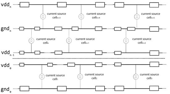
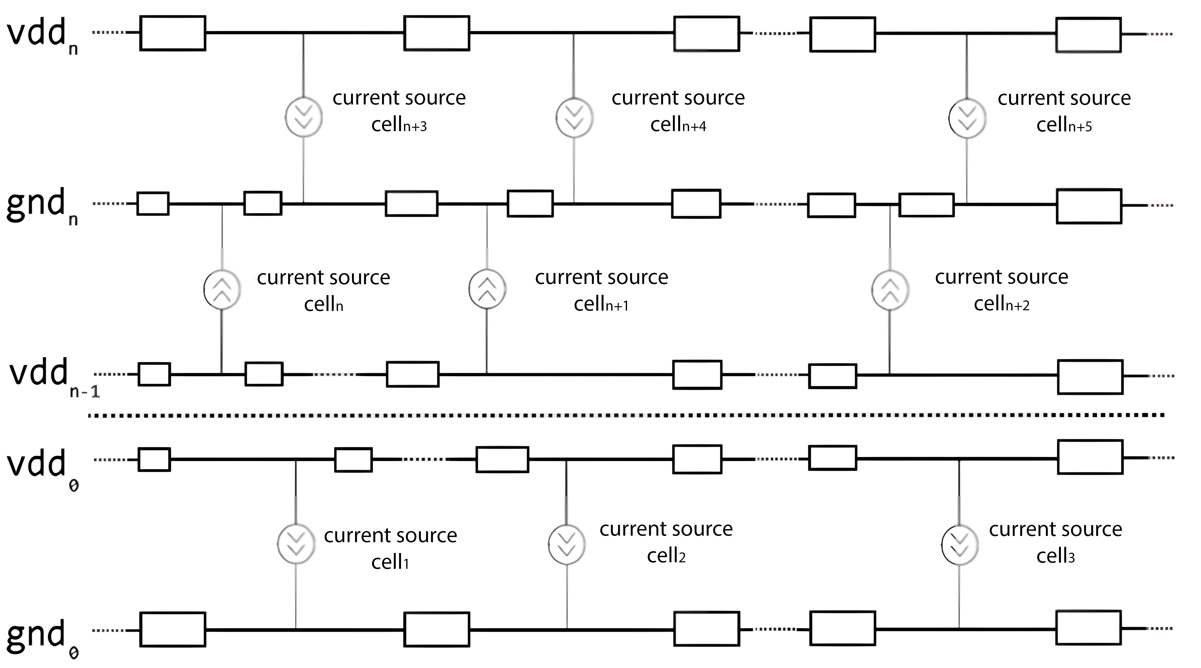
To simplify a circuit analysis, the method of static analysis for the IR drop is used, which takes into account the average number of transistor switches per a clock cycle. This method is less accurate than the dynamic one, but the analysis time is significantly reduced. To carry out the static IR drop analysis, a circuit topology is represented as a simplified equivalent circuit model (Figure 1), which includes a resistor grid representation of power and ground rails, as well as the DC source representation of standard cells.

Figure 1. Equivalent model of design for performing the IR drop analysis.

The main stages for constructing an equivalent model and performing static IR drop analysis are as follows:

•

Obtain a grid of resistors equivalent to the metal connections of the circuit;

•

Calculate the average power consumption of each standard cell to get DC sources and build an equivalent circuit model;

•

Calculate the current in each section of the circuit by solving the linear equation system;

•

Calculate the voltage in each section of the circuit:

$$V=I\times R.$$

(1)

The goal of simulating an equivalent circuit model is to calculate voltages at all nodes of the power grid. Traditionally, this problem is approached using a method for solving systems of linear equations of the form

$$G\times V=J$$

(2)

where

$G$ is the conductance matrix;

$V$ is the calculated voltage value at each node;

$J$ is the current matrix.

The problem with this approach is the calculation time, which rapidly increases with the increase in the number of power grid nodes in the circuit. Nowadays, machine learning (ML) methods have become widespread in Electronic Design Automation [4]; using them to solve computational problems when analyzing the static IR drop effect can be promising [5].

ML models have already been tried as a tool for static IR drop analysis [6,7,8]. As part of these research activities, a solution to calculate the static voltage drop across the entire chip based on the power distribution map along the interconnect grid and power grid was proposed [6]. An ML model for quickly exploring the IR drop analysis (reducing analysis time by several times compared to commercial CAD systems) was developed [8]. A major challenge in using ML models is generating a database for training. To fully train an ML model, an analysis of all possible variants of the studied circuits is needed. Differences in the circuits under study may begin with the design technology and end with the size and options for constructing the resistive power delivery network (PDN).

The following parts of the article are organized as set out below:

• The architecture and methodology for the training of ML models is described;
• The methodology for collecting training data to expand the dataset is investigated;
• A method for generating two-dimensional data from the initial SPICE (Simulation Program with Integrated Circuit Emphasis) description of power buses is proposed;
• A comparison of the speed and accuracy of the proposed method with the SPICE simulation is made.

The proposed solution was ranked in the TOP 3 of the ICCAD Contest (Problem C).

2. Materials and Methods

Problem Formulation and Initial Dataset (ICCAD Contest)

In 2023, the ICCAD Contest [9] was held as part of the ICCAD conference [10]. This competition has been held annually for many years; every time, modern problems in microelectronics are put forward, and the proposed solutions are analyzed. While recent advancements have explored ML for IR drop analysis, significant challenges remain in capturing the intricate resistive topologies of modern power delivery networks (PDNs). This work addresses these gaps with two primary contributions: (1) a novel SPICE-to-image conversion flow that utilizes Gaussian-blurred resistance maps to preserve PDN topology better than standard density maps, and (2) an asymmetric loss function designed to prioritize the detection of critical voltage “hotspots,” essential for design closure.

The global task was to develop an ML model that could estimate the static IR drop effect over the entire circuit area in a short time. The input data for ML model training are four matrices for each circuit: the matrix of the current sources, matrix of the effective distances to voltage sources, matrix of the resistive grid density (PDN density map), and matrix of the IR drop values. A detailed description of each of the matrices is given below.

As training data, the contest organizers provided 10 real circuits and 100 generated circuits; the information about each of them was presented as four files: current_map.csv, eff_dist_map.csv, pdn_density_map.csv, and ir_drop_map.csv. Also, for each circuit, a description of the PDN (power delivery network) in the SPICE format was given.

During the preliminary study, it was discovered that such a number of circuits is not enough to fully train an ML model; therefore, as part of this work, a flow to generate the additional training data (both artificially generated from the presented ten circuits and synthesized from RTL (Register Transfer Level) using the OpenROAD flow) was implemented.

3. Problem Structure Analysis

Before describing the workflow, it is necessary to formulate the IR drop analysis as a learning problem. The static IR drop is governed by the system of linear equations $G\cdot V=J$, where $G$ is the conductance matrix, $V$ is the voltage vector, and $J$ is the current vector. Traditionally, solving for $V$ requires inverting $G$ or using iterative solvers, which scales poorly ($O\left(N^3\right)$ or super-linear) as the number of nodes $N$ increases.

In this work, we approximate the inverse operator $V=f(J, G, \mathrm{t}\mathrm{o}\mathrm{p}\mathrm{o}\mathrm{l}\mathrm{o}\mathrm{g}\mathrm{y})$ using a neural network. This approach is justified by the physical properties of the power delivery network (PDN).

Locality: The voltage at a specific node is primarily determined by its local neighborhood of resistors and current sources, though global dependencies exist. Convolutional networks naturally exploit this spatial locality.

Regularity: The PDN is topologically similar to a regular grid (image), making CNNs significantly more computationally efficient ($\mathrm{O}\left(1\right)$ inference time per pixel) compared to Graph Neural Networks (GNNs) or numerical solvers.

Global Attention: To capture long-range dependencies (e.g., a voltage source far from a sink) we utilize architectures like MaxVit that combine local convolutions with global attention mechanisms.

4. Proposed Workflow for IR Drop Prediction

The distribution of the static IR drop values on the power grid network in a chip depends on the following three factors [11]:

•

The location/distribution of all voltage sources (power pads) in the design;

•

The topology of the ground and power network; the resistance values of each resistor (via/metal layer) in the network;

•

The distribution of current sources in the design.

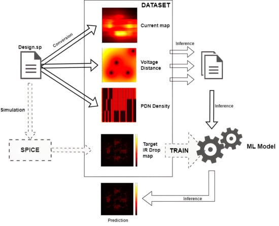
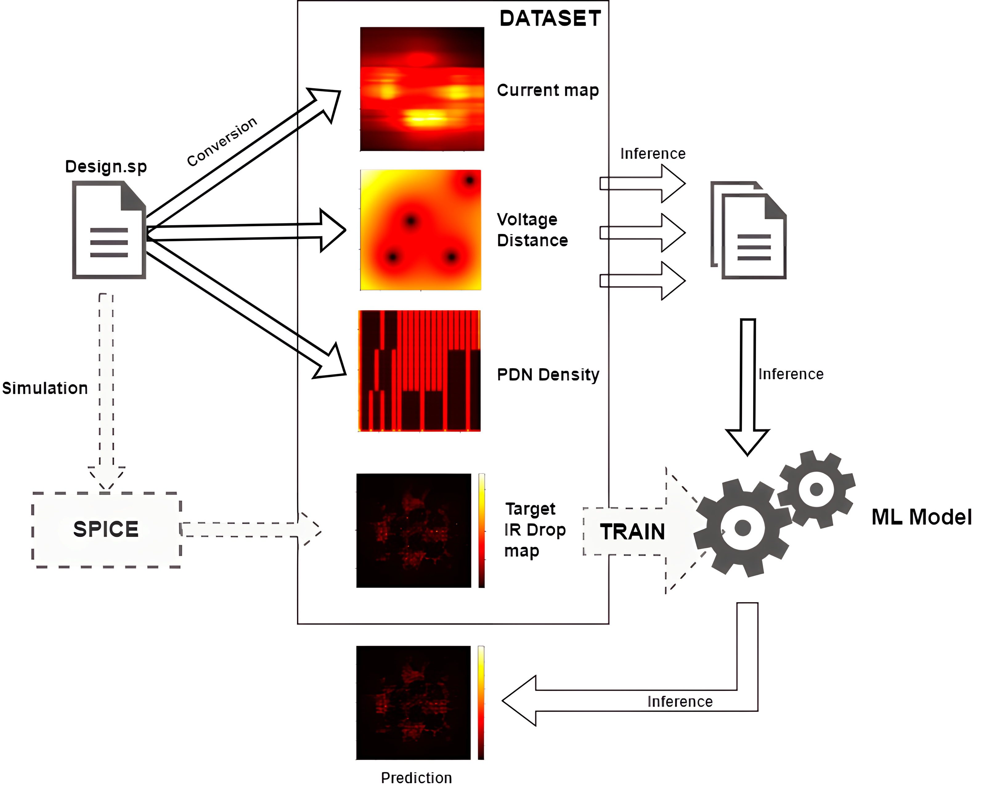
Each of the named factors is associated with the floorplan and, therefore, can be represented as an image. The final result of the IR drop analysis is also an image, which allows us to use rich experience in developing various ML models for image processing. In this work, we propose a flow for training and applying (inferential) models to analyze the IR drop on ground and power circuits (Figure 2).

Figure 2. ML model training route for the IR drop prediction.

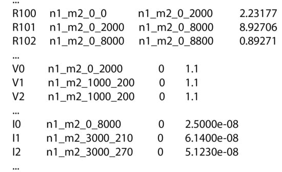
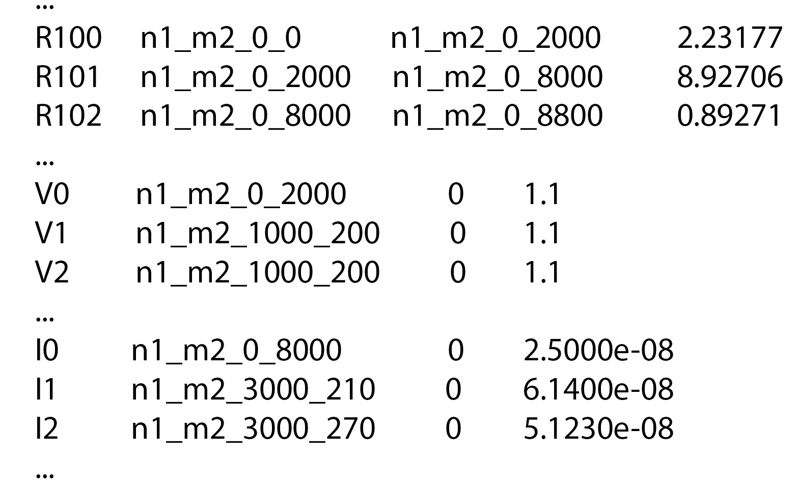
The developed flow receives an input file describing the PDN, which is a SPICE file with external voltage sources, current sources simulating standard cells and resistors that determine the resistance of metal wires. Net names encode their coordinates in the network floorplan, which makes it possible to fully recreate the PDN floorplan (Figure 3).

Figure 3. SPICE netlist example.

The input file is passed to the converter, which should generate images that reflect all three factors enumerated at the beginning of this section. After this, the images are fed to the predictive model, which produces the IR drop map on the power grid network. Training the model comes down to generating a dataset in which the results of the SPICE simulation of a large set of circuits will act as reference values of the IR drop maps; after this, the model learns to predict the IR drop values in all the nodes of the circuit (Figure 2).

A similar approach associated with converting the PDN into images has already been proposed in several scientific works [6,7,12,13]. For example, in [6], the above three characteristics are represented as three distributions, where the distribution of current sources is modeled as a current map; the topology of metal wires is modeled as a function of density (the distance between power strips per unit area) in different regions; and the distribution of voltage sources is modeled as an effective distance map, which represents the distance from each circuit node to the power source node. In the paper, the use of a convolutional neural network and U-Net [14] is proposed. With the latter, the models trained on a diverse set of the described data (three inputs and one output) can be used for the IR drop prediction.

In this work, we propose a similar approach, differing in the architecture of the neural network, SPICE file-to-image converters, and some aspects of post processing of the neural network results. The Section 5 describes the principles of generating images for the training and inference of neural networks from the SPICE files describing the chip’s PDN.

5. SPICE-to-Image Conversion for Feature Engineering

All the three input images provided for each circuit (as well as the output IR drop) have the same resolution, which is proportional to the actual die size. In the contest, the image size in pixels is equal to the design size in micrometers. One pixel represents the chip area of one square micrometer. However, in the provided SPICE file (Figure 3) containing information about resistances, the voltage sources, current sources, and circuit coordinates are scaled with a factor of 2000. This factor must be taken into account when converting. In other words, one pixel of the resulting image contains 2000 arbitrary units along the x-axis and 2000 arbitrary units along the y-axis.

5.1. Constructing an Effective Distance Map

The way to construct an effective distance map is to map the actual matrix of the voltage sources into a matrix that will not only be compressed in size but also show how far or close each cell of the matrix is placed. This mapping serves as a heuristic proxy for the impedance path from a node to the power supply. We utilize the inverse sum of Euclidean distances because the influence of a voltage source decays with distance. While the exact resistance paths depend on the specific mesh topology, the Euclidean distance provides a robust approximation for uniform grids, allowing the model to estimate how “well-supplied” a specific region is.

This can be done using the following algorithm:

• Initially, the display step along the axes is selected: $X, Y$—$stepX$ and $stepY$, respectively. If the size of the original matrix is known, the size of the compressed matrix will be calculated:

$${\mathit{w}}^{\prime }=\left(\frac{\mathit{w}}{\mathit{s}\mathit{t}\mathit{e}\mathit{p}\mathit{X}}\right)+1,{\mathit{h}}^{\prime }=\left(\frac{\mathit{h}}{\mathit{s}\mathit{t}\mathit{e}\mathit{p}\mathit{Y}}\right)+1.$$

(3)

2.

The algorithm iterates through all the cells of the ($w^{\prime },h^{\prime }$) matrix. For each cell, the inverse sum of the Euclidean distance to all the voltage sources is calculated:

$$S=\sum _0^n{\displaystyle \frac{1}{\sqrt{{\left(x_n-x\right)}^2+{\left(y_n-y\right)}^2}}},$$

(4)

where

$n$ is the number of voltage sources;

$x,y$ are the coordinates of the cell in question;

$x_n,y_n$ are the coordinates of each voltage source in the design.

While the Manhattan distance is often intuitive for orthogonal routing, the Euclidean distance was selected for Equation (4) to model the omnidirectional “field-like” propagation of potential from power pads through the dense resistive mesh. Preliminary tests indicated that the radial symmetry of the Euclidean distance provided a more stable gradient for the neural network during the initial stages of training.

3.

After calculating the sum, each cell is assigned an effective distance value:

$$cell={\displaystyle \frac{S·\left(stepX+stepY\right)}{2}}.$$

(5)

Therefore, if the cell is close to the voltage source, the value in the matrix is high, and vice versa.

5.2. Constructing the Power Supply Resistance Map

In the contest, to represent the ground and power network data, the PDN density map was accepted, which reflects the PDN topology and resistance of each resistor in this network [10]. The density map is modeled as a function of density (the distance between power strips per unit area) of the power grid in different regions of the chip.

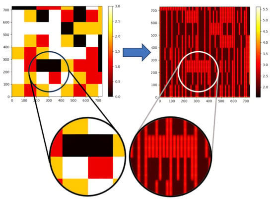
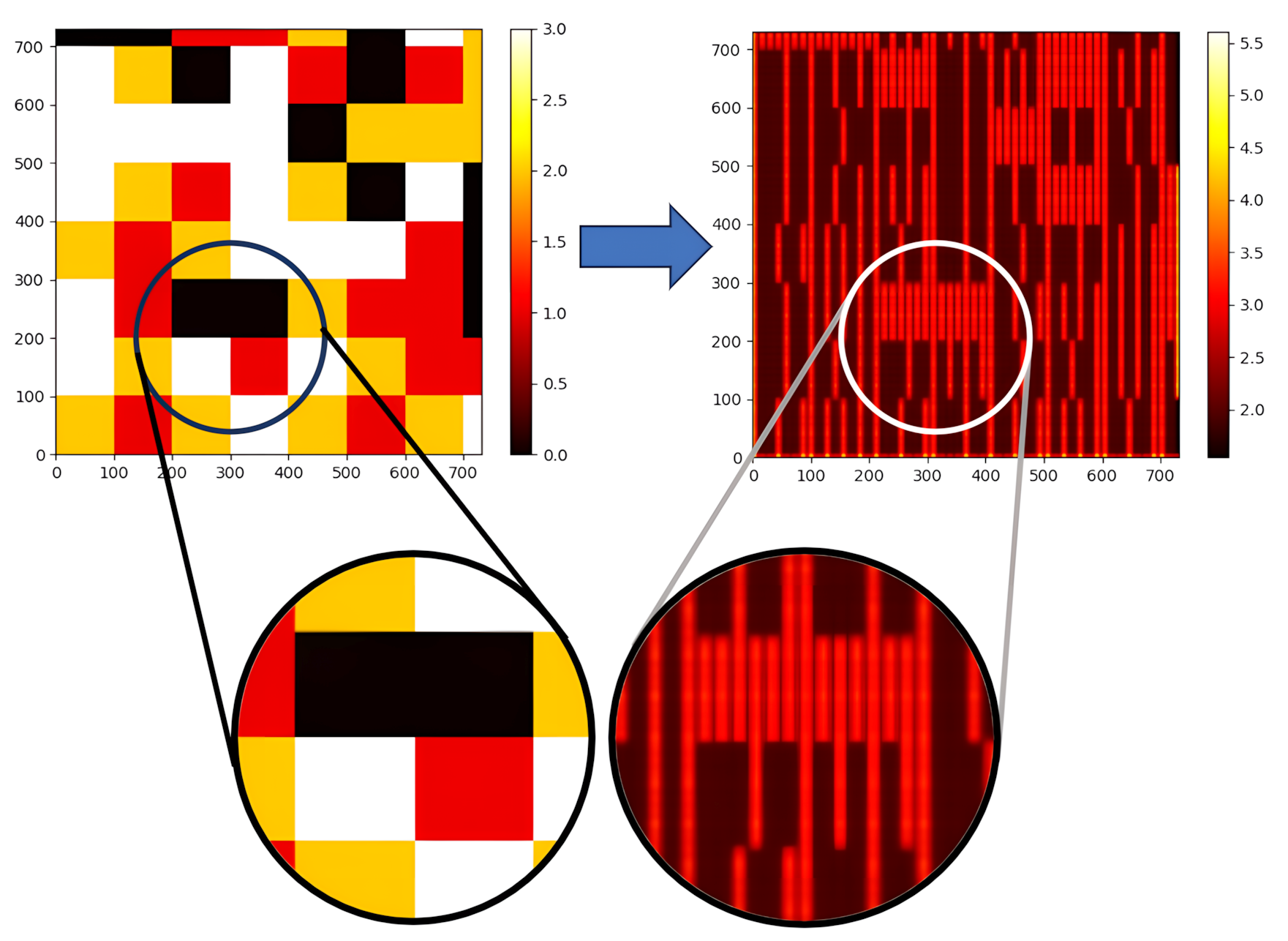
However, we propose to use the power network floorplan itself. The resulting map directly reflects the distribution of the resistance of the PDN metal wires over the chip area. This allows for a more accurate modeling of the IR drop; also, the model can be used on highly irregular power networks. A standard PDN density map only reflects the spatial density of metal stripes, potentially smoothing out critical details. In contrast, our proposed resistance map directly encodes the electrical resistance values. This allows the model to detect specific local bottlenecks—such as missing vias or routing blockages—that would otherwise be invisible in a density representation. The difference between this map and the PDN density map is shown in Figure 4.

Figure 4. Distribution map of the resistive power network (density map—left, resistance map—right).

To obtain the PDN resistance map, it is necessary to:

• Extract the node coordinates $x1,y1,x2,y2$ and resistance values for all the resistors from the SPICE file describing the circuit.
• Create the empty matrix of size $x_{width}\times y_{width}$, where $x_{width}$ and $y_{width}$ are calculated based on the core size and grid step ($stepX$ and $stepY$) equal to 2000.
• Add the value of each resistor to the matrix cells corresponding to the coordinates of the ends of the resistor divided by the grid pitch.
• Apply Gaussian blur to the matrix to smooth the image. We used gaussian_filter with $sigma=4$ from the scipy.ndimage module.

Thus, the result is the PDN topology map reflecting the distribution of resistors over the chip area. This map is used as one of the input features for ML model training.

5.3. Obtaining the Power Supply Map

The main idea of the techniques for building the current source map is mapping the real matrix with current sources into some compressed version, while minimizing possible information loss. The following algorithm can be used:

• Select a mapping step along the $x,y$ axes: $x,y$—$stepX$ and $stepY$, respectively. If the size of the original matrix is known, the size of the compressed matrix will be calculated:

$${\mathit{w}}^{\prime }=\left(\frac{w}{\mathit{s}\mathit{t}\mathit{e}\mathit{p}\mathit{X}}\right)+1, {\mathit{h}}^{\prime }=\left(\frac{\mathit{h}}{\mathit{s}\mathit{t}\mathit{e}\mathit{p}\mathit{Y}}\right)+1.$$

(6)

2.

Traverse the real matrix through the cells that store the information about the current sources. First, the position of each current source in the compressed matrix is calculated:

$${\mathit{x}}^{\prime }=\left(\frac{\mathit{x}}{\mathit{s}\mathit{t}\mathit{e}\mathit{p}\mathit{X}}\right), {\mathit{y}}^{\prime }=\left(\frac{\mathit{y}}{\mathit{s}\mathit{t}\mathit{e}\mathit{p}\mathit{Y}}\right).$$

(7)

If the current source coordinates do not align perfectly with the center of a grid cell, simple binning would result in spatial quantization errors. To address this, we apply an area-based distribution (anti-aliasing). The current value is distributed among the nearest grid cells proportional to the overlap area between the “virtual” cell of the current source and the underlying grid cells. This ensures that the total current is conserved and that spatial precision is maintained before the Gaussian blur is applied.

3.

Determine the impact of the given current source on the surrounding cells; this should consider the intersection area of a cell with the center at point ($xstepX-0.5,ystepY-0.5$), size $(1, 1)$, with the cells surrounding the cell ($x^{\prime },y^{\prime }$) within one cell radius. The cell intersection area is then multiplied by the numerical value of the current source and added to the intersecting cell.

4.

Pass the resulting compressed matrix through a Gaussian filter to achieve a more uniform distribution of the values in the empty cells.

6. Dataset Generation and Expansion

The major issue faced by the developers of ML models for solving problems in the field of physical synthesis is the lack of training data. The same is true for the studied problem. The authors of the contest provided open access to 100 generated circuits for training and 10 real circuits for debugging the proposed solution, and the organizers of the contest kept hidden another 10 real circuits that were reserved for the internal testing of the solutions [10]. Hidden circuits are needed to ensure that the developed models are not trained on these real circuits. These hidden circuits were used to form the final contest leaderboard. A total of 10 real circuits and 100 generated circuits are not enough to train a good model. Therefore, it was necessary to search for and prepare additional data for training. It was discovered that the test circuits were synthesized using Nangate45 technology [15], since the generated power grid using this technology was similar to the data provided by the organizers. The organizers recommended using circuits built with the generative neural network BeGAN for training [16,17].

In this work, new circuits were generated from the existing ones, and the floorplans of several real circuits were synthesized using Nangate45 technology with the help of the automated physical synthesis flow OpenROAD [18,19].

To ensure a rigorous evaluation and prevent data leakage, the dataset split was performed at the Design ID level. All patches derived from a specific source circuit (whether real or synthetic variant) are confined strictly to either the training or the validation set. This ensures the model is evaluated on unseen power grid topologies, rather than simply memorizing the texture of a floorplan seen during training.

6.1. Algorithm for Obtaining the IR Drop Map

The result of the physical synthesis stage is the design floorplan presented in the standard DEF (Design Exchange Format). Then, using the PDNSim program included in OpenROAD [20], the SPICE netlist was generated. Using the SPICE simulation, the voltage values at each node of the resistive mesh were obtained; these values were finally converted into reference values for the IR drop at each node.

6.2. Algorithm for Generating New Circuits from the Preexisting Ones

To expand the training dataset based on the existing circuits, several approaches were used:

• Moving current sources to new positions.
• Increasing the number of current sources.
• Changing the numerical values of current sources.

To generate new circuits, the above approaches were applied sequentially. If the current sources have already been moved in all possible ways, adding new sources is launched. As soon as all the nodes on the lower metallization layer are connected to current sources, changing their values (until an IR drop value comparable in order to other circuits is reached) can be started.

All the circuit modifications are based on the input SPICE description; the output format is also SPICE. During the generation process nodal analysis [21], the standard method in circuit design to calculate the voltage drop values was used.

The main advantage of this method is that it enables the generation of many new circuit variants, which can also be solved using the nodal potential method [22] without changing the resistive mesh.

6.3. New Tests Based on the Real Circuits

To expand the set of data required for ML model training, an additional set of real circuits was generated. Several training circuits were designed using the Nangate45 technology [15].

The main stages in new data building for neural network training were:

• Carrying out the physical synthesis of the circuits from the test set for the Nangate45 technology and circuits from the ISCAS85 set of benchmarks [23] using the open design flow OpenROAD.
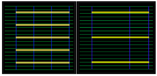
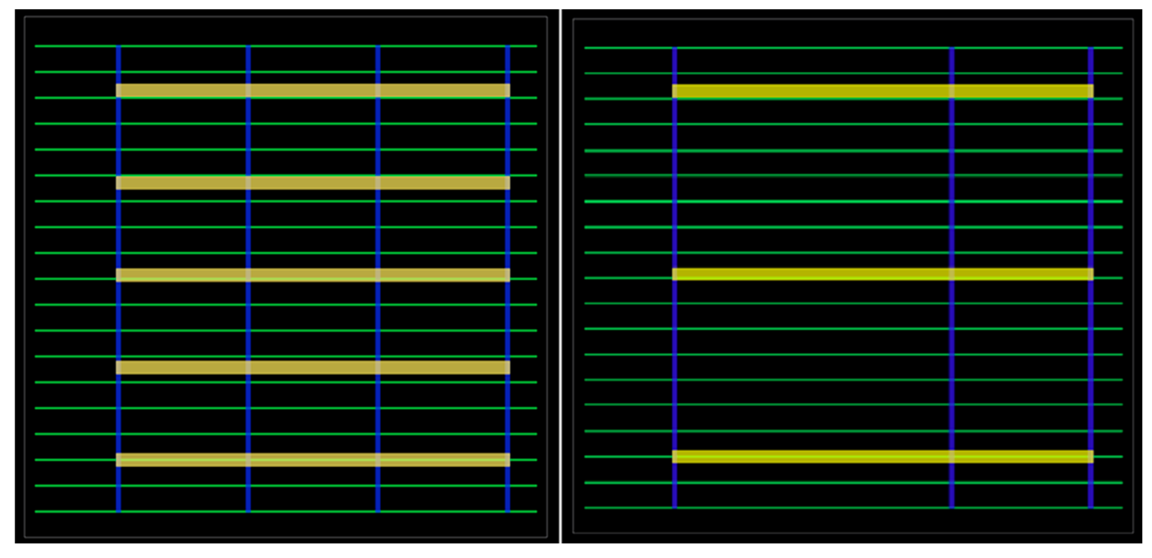
• Generating multiple variants of real examples of circuits based on synthesized ones by changing the resistive PDN on the principle of removing some power rails. Removing a limited number of vertical and horizontal top-level power rails does not lead to functional failures; so, such circuits can be used for training.
  For example, Figure 5 shows the floorplan views before and after upgrading the power grid for one of the circuits from the ISCAS85 set [23], and Figure 6 shows the corresponding IR drop maps.
  

  Figure 5. Power network for the c7552 design from the ISCAS85 test circuit set ((left)—before power net conversion, (right)—after power net conversion).
  

  Figure 6. IR drop distribution map for design c7552 ((left)—distribution map with the unchanged power net, (right)—distribution map with the changed power net).

3.

Generating a random number of voltage sources placed in the floorplan at permitted coordinates (so, such circuits can also be treated as real ones).

4.

Building SPICE netlists for the generated set of circuits and simulating them to get heat maps with the IR drop values in each circuit node as a .csv file: ir_drop_map.csv.

Thus, as the result of data generation, some sets of circuits were built, where each circuit is described by four .csv files needed for training ML models of neural networks.

7. Machine Learning Model Architecture and Training

The architecture of the ML model was selected. U-Net [14] and FPN [24] architectures with different encoders were tested. Convolutional neural networks from the EfficientNet family [25] and Multi-Axis Vision Transformers—MaxVit [26] were used as encoders. The selection of EfficientNet and MaxVit encoders was driven by the specific physical nature of IR drop propagation. Standard CNNs often struggle with long-range dependencies due to their localized receptive fields. In contrast, MaxViT (Multi-Axis Vision Transformer) utilizes global attention mechanisms that are better suited for capturing the long-distance electrical influence of power pads on distant nodes in a large resistive mesh. EfficientNetB5 was selected for its balanced scaling of depth and resolution, allowing for high-fidelity feature extraction from the 2D resistance and current maps. Their comparison on the validation dataset showed that MaxVit has a higher MAE score than EfficientNetB5. The superior performance of MaxVit can be attributed to its hybrid architecture. While standard CNNs (like EfficientNet) excel at processing local features, they struggle with global context. IR drop is a global phenomenon where a current spike in one region can affect the voltage levels across the chip. MaxVit utilizes Multi-Axis Attention to capture these global interactions, providing a theoretical advantage over purely convolutional encoders. We also had to select an input size for the neural network. Resizing source images results in a loss of information; so, the images should be passed pixel to pixel. But it is not necessary to send the entire image; it is enough to provide a small part of it. The maximum training circuit size in pixels was $930\times 930$. Modern neural networks for transformer-based image classification rarely accept images larger than $512\times 512$ pixels as input; the typical input size is usually $224\times 224$ pixels. So, we tried different image sizes from $128\times 128$ to $512\times 512$ pixels. In our experiments, the maximum quality was achieved at large sizes. Apparently, this is because the neural network got more information to predict the IR drop values this way. If the image was smaller than the specified size, it was padded with zeros to the specified size.

The following actions were used for data augmentation:

• Selecting a random patch of the desired size from the image.
• Random rotation by 0/90/180/270 degrees.
• Random vertical/horizontal reflection.

At the stage of inference, when analyzing a given circuit, it was first converted into an image and then analyzed for the IR drop value using the floating window method. The window size was $512\times 512$ pixels (that is, equal to the input of the neural network); the step could be varied. Namely, the smaller the step, the higher the accuracy, but the lower the operating speed. We use a stride of 256 pixels (50% overlap). Also, to improve the accuracy, the Test Time Augmentation method [27] was used. The image was rotated by 90 degrees and reflected in all the eight possible positions, and the result was averaged. Alternatively, only some of the eight positions can be used, which helps to find some balance between accuracy and speed.

During training, we have encountered the case that the F1 score for test examples is sometimes equal to zero, but the MAE score value is low. This is due to the peculiarity of calculating the F1 score. When the value of 90% of the maximum is $N$, then—if we predict a value less than $N$—we get a False Negative, and—if we predict a value greater than $N$—we get a True Positive and thereby improve the F1 score. However, from the point of view of the MAE score, nothing changes. For the large IR drop values, it is more profitable to predict the IR drop value with some margin upward and avoid the underestimated IR drop values. Therefore, the loss function was modified as follows:

$$\mathrm{if} pred<true, \mathrm{then} loss=K·MAE,$$

(8)

$$\mathrm{if} pred\ge true, \mathrm{then} loss=MAE.$$

(9)

In the experiments, the coefficient $K$ was set equal to 2. The coefficient K = 2 was determined through a heuristic sensitivity analysis aimed at optimizing the F1 score. By weighting the Mean Absolute Error (MAE) more heavily when the model underestimates the IR drop (pred < true), the model is incentivized to produce conservative estimates that are safer for timing and functional verification.

Additionally, at the inference stage, the values greater than 90% of the maximum IR drop were multiplied by the correction factor of $1.05$. This also improved the F1 score for validation and at the same time almost did not worsen the MAE score.

The problem that the training did not converge if the values were given in absolute terms was faced. Apparently, the reason for it was that the calculation error began to exceed the desired values, or that we used mixed precision during the training. Therefore, the values of both the input data and the desired IR drop were scaled: the current sources were multiplied by ${10}^8$, the effective distance map was multiplied by 100 and the PDN density map was multiplied by 100. The IR drop values were multiplied by ${10}^5$. Throughout this work, the MAE values are reported in scaled units ${10}^{-5}$ V.

Experimental Setup

To train the model, one single NVIDIA A6000 48 GB GPU, 256 GB RAM, 16-cores AMD Threadripper CPU, and storage 1 TB SSD hard drive were used. It is possible to use GPU with less memory, only the batch size (and probably learning rate) must be adjusted accordingly.

8. Evaluation Metrics

In the work frame of the contest, two quality metrics were proposed: MAE (Mean Absolute Error) and F1 score [28]. The MAE score was considered the most important when assessing the IR drop prediction quality; its contribution to the overall quality score was set to 60%. The F1 score contributed 30%, and the remaining 10% was contributed by the computation speed. The MAE score evaluates the overall quality of the solution across the entire design. The F1 score evaluates the quality only in critical sections of the circuit with the maximum IR drop value. It is important for chip designers to know the coordinates in the floorplan where the voltage drop is maximum. In these points, it is necessary to solve the problem of large voltage drop. All other circuit locations have less IR drop; thus, calculation accuracy plays much smaller role there.

8.1. MAE Score

The MAE, or Mean Absolute Error [29], is the average of the absolute difference between the predicted and actual value calculated for each example in the dataset. The goal is to minimize the MAE score.

Example: Let us take a 2 × 2 matrix for clarity. Let us assume we obtained the following IR drop values

$$\begin{gathered} 2.1 6.4 \\ 3.8 0.1 \end{gathered}$$

while the actual values of IR drop are

$$\begin{gathered} 2.5 5.3 \\ 4.9 0.0 \end{gathered}$$

Then, the MAE matrix will look as follows:

$$\begin{gathered} 0.4 1.1 \\ 1.1 0.1 \end{gathered}$$

The MAE score after averaging will be equal to

$$\mathrm{M}\mathrm{A}\mathrm{E}=0.675.$$

This is the average error value over the entire IR drop matrix.

8.2. F1 Score

The F1 score is a binary classification metric [30]. In this task, it uses 10% of the maximum IR drop of each circuit as the classification threshold. The formulas for calculating the F1 score are as follows:

$$F1=(2\times Precision\times Recall)/(Precision+Recall),$$

(10)

where $Precision={\displaystyle \frac{TP}{TP+FP}}, Recall={\displaystyle \frac{TP}{TP+FN}}$.

On the IR drop map, the value 1 (True) marks areas where the IR drop is higher than 90% of the maximum for the given circuit. We have to find such areas as accurately as possible. The more accurate the results, the higher the F1 score.

According to the example from the Section 8.1, the maximum IR drop value for the matrix is $5.3$. If we take 90% of it, then the value would be $4.77$. Thus, all the values greater than $4.77$ in both the predicted matrix and the real matrix will be set to 1, and the remaining values will be set to 0.

So, the hotspot matrix for the predicted matrix will be

$$\begin{gathered} 0 1 \\ 0 0 \end{gathered}$$

For the real matrix,

$$\begin{gathered} 0 1 \\ 1 0 \end{gathered}$$

Thus,

$$TP=1, TN=2, FP=0, FN=1.$$

Using the formulas, the F1 score can be calculated as

$$Precision=1/(1+0)=1,$$

(11)

$$Recall=1⁄\left(\right(1+1) )=0.5,$$

(12)

$$F1=(2\ast 1\ast 0.5)⁄\left(\right(1+0.5\left)\right)=0.67.$$

(13)

9. Simulated Results and Discussion

To test the operation speed and accuracy, the data provided by the organizers of ICCAD were used. There were 10 real circuits (Table 1). The speed and accuracy of the SPICE simulator NGSPICE [31] and the proposed neural network model are compared.

Table 1. Test circuit sizes.

Test Circuit Name	Size, um2	Number of Resistors
testcase1	298 × 298	24,087
testcase2	298 × 298	22,327
testcase3	930 × 930	228,439
testcase4	930 × 930	214,889
testcase5	641 × 641	110,465
testcase6	641 × 641	102,525
testcase11	204 × 204	10,859
testcase12	204 × 204	10,407
testcase17	566 × 566	84,044
testcase18	566 × 566	80,038

To ensure rigorous validation and prevent data leakage, the dataset was partitioned at the circuit level. All augmented derivatives of a specific base circuit (e.g., “testcase1”) were strictly confined to the same fold during K-Fold cross-validation. This ensures that the model was never evaluated on unseen variations in a topology it had encountered during training, thereby providing a true measure of the model’s ability to generalize to new chip floorplans.

Since the neural network was trained using K-Fold validation [32] with the parameter k = 5, five models were created as the result. An Out-of-Fold scheme was used for the value prediction; that is, for each of the five models, the values were predicted for the circuits that were not involved in training. The test results are shown in Table 2. According to the table, the time to calculate the voltage drop using the ML model is less than 1.0 (even for large circuits). Most of the time is spent on the conversion of the SPICE description into a 2D matrix. This operation can be optimized, which will give an additional increase in speed. In this work, no optimization was done.

Table 2. Results of speed comparison between the NGSPICE and ML model.

Test Circuit Name	$\mathbf{Time}, \mathbf{s}$			Speed-Up Compared to NGSPICE (× Times)	$\mathbf{MAE} \mathbf{Score}\times {10}^{-5}$	F1 Score
	NGSPICE	SPICE Netlist to Matrix Conversion	ML Model
testcase1	5.8	0.9	0.2	5.2	9.30	0.62
testcase2	4.7	0.9	0.1	4.7	14.31	0.87
testcase3	1230.3	45.4	0.8	26.6	4.84	0.75
testcase4	966.9	45.2	0.8	21	10.18	0.63
testcase5	170.3	11.9	0.4	13.8	6.10	0.81
testcase6	125.9	11.9	0.4	10.1	10.21	0.60
testcase11	1.1	0.5	0.4	1.2	10.59	0.52
testcase12	1.1	0.5	0.4	1.2	14.27	0.62
testcase17	83.6	7.3	0.6	10.5	3.41	0.69
testcase18	75.8	7.4	0.7	9.3	4.39	0.79

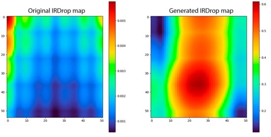
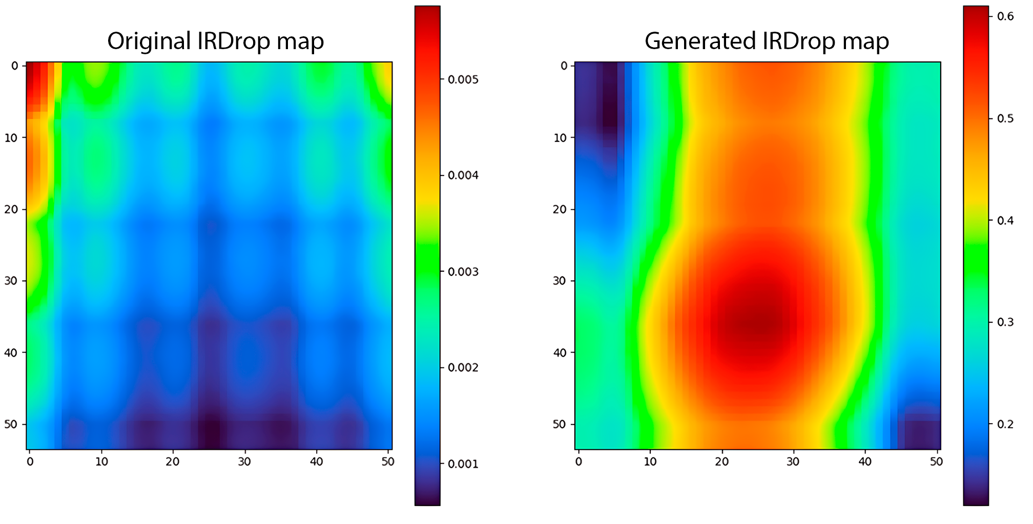
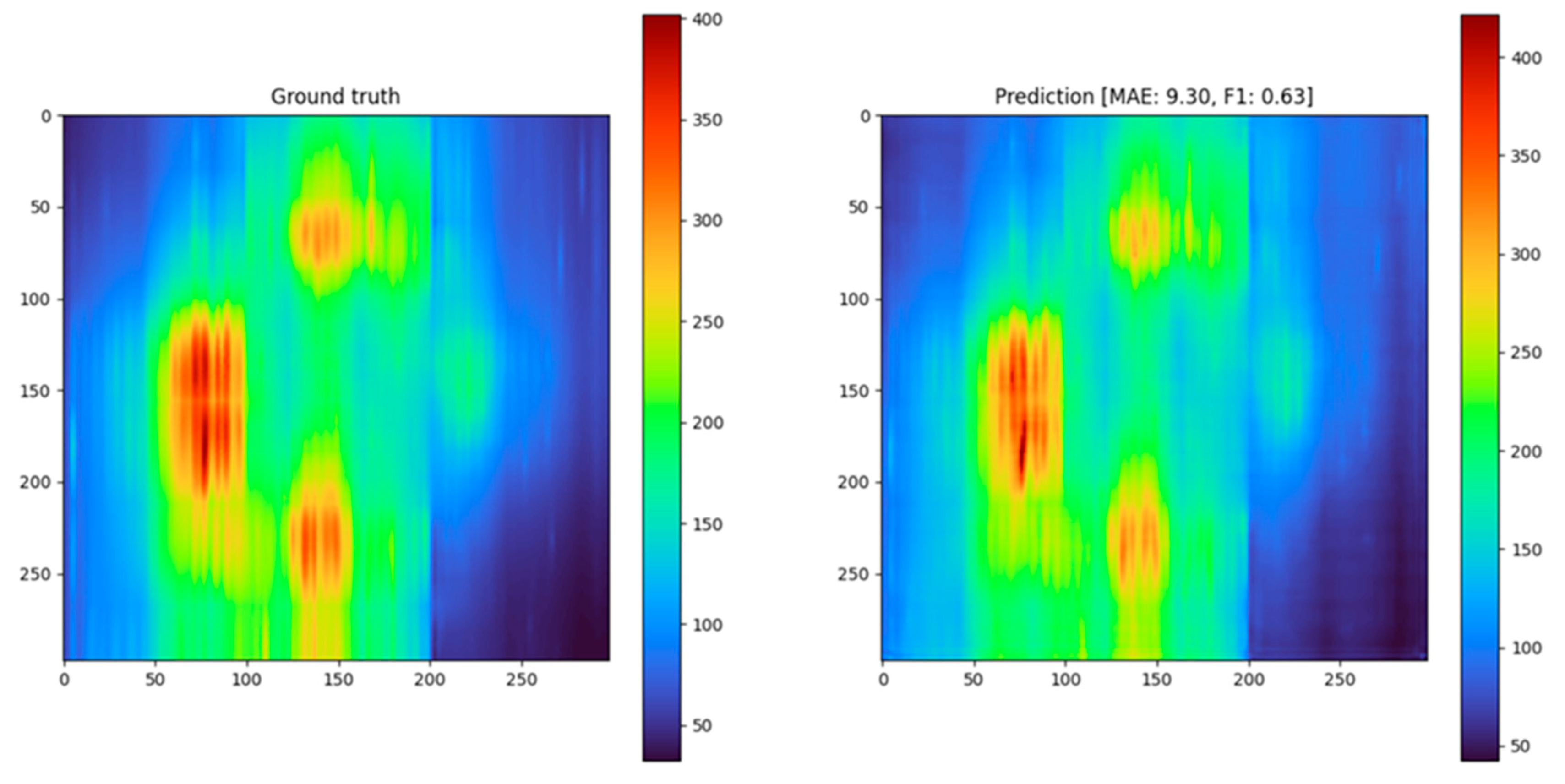
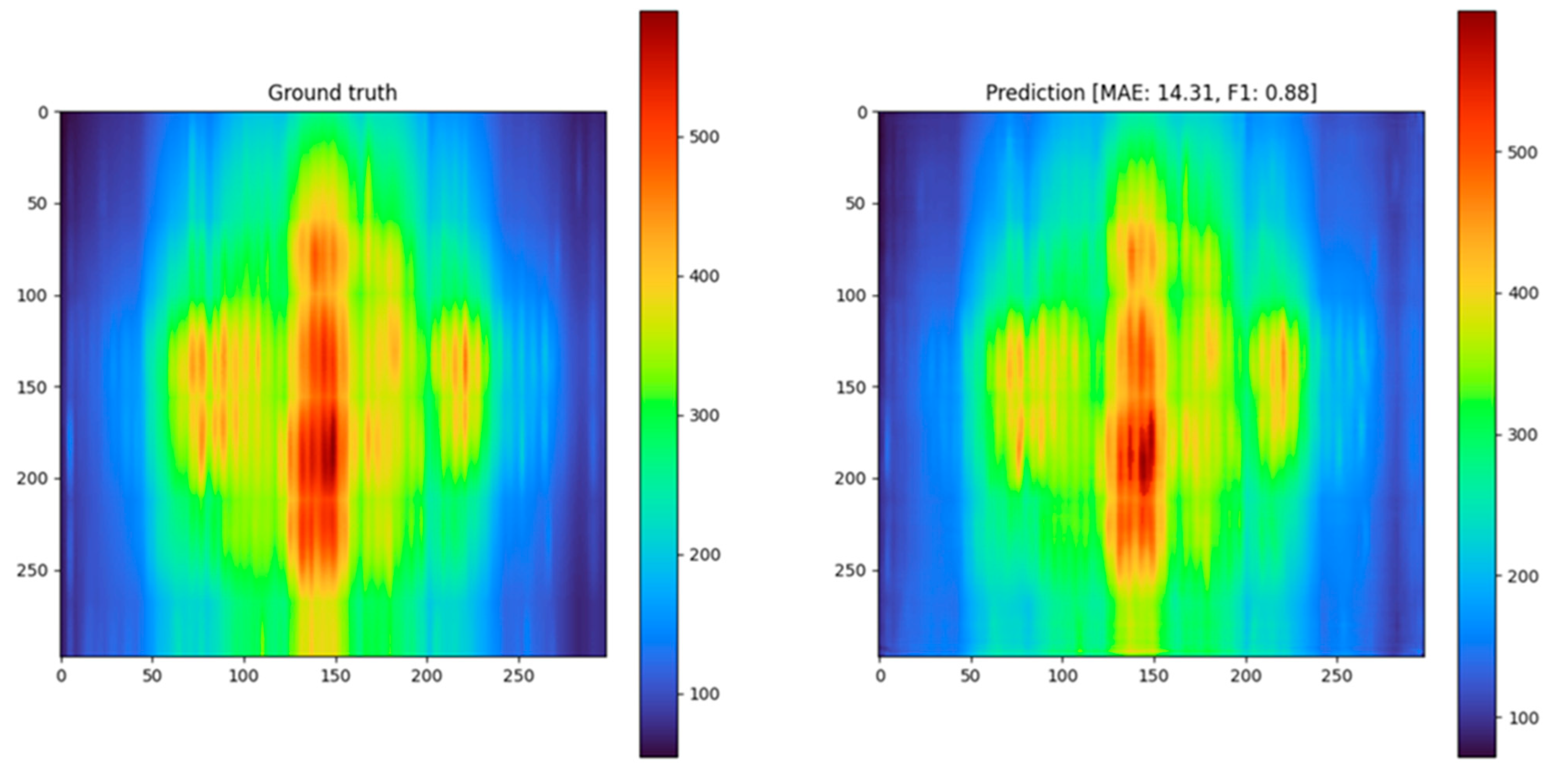
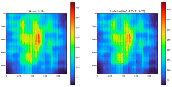
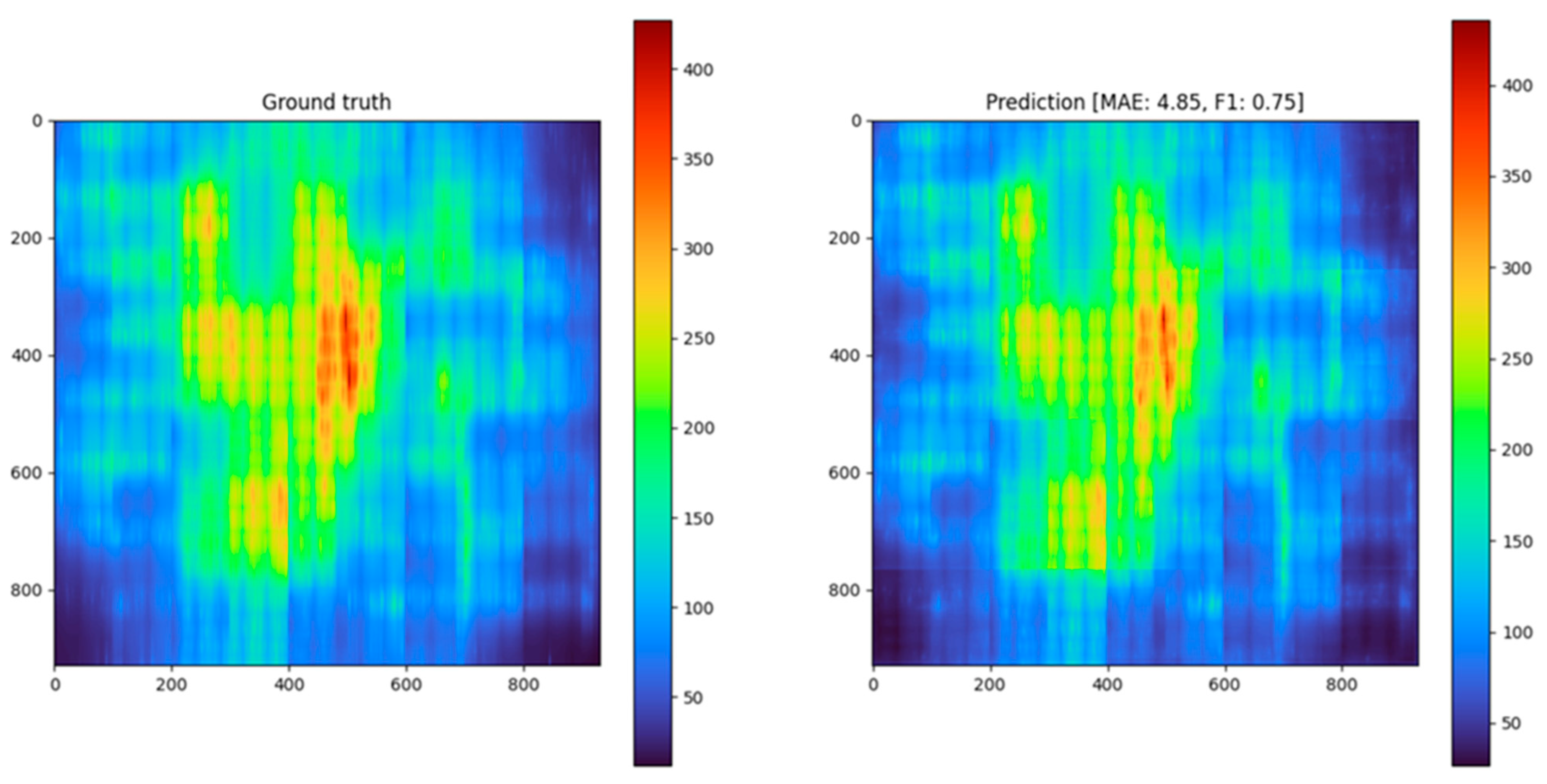
The results of comparing the real IR drop map with the predicted one for several test circuits are shown in Figure 7, Figure 8 and Figure 9.

Figure 7. Real (left) and predicted (right) IR drop for testcase1 design (values of IR drop need to be multiplied by ${10}^{-5}$).

Figure 8. Real (left) and predicted (right) IR drop for testcase2 design (values of IR drop need to be multiplied by ${10}^{-5}$).

Figure 9. Real (left) and predicted (right) IR drop for testcase3 design (values of IR drop need to be multiplied by ${10}^{-5}$).

The comparative performance of the proposed method against the first- and second-place solutions from the ICCAD 2023 Contest (Problem C) is summarized in Table 3 and Table 4. While our approach officially secured a TOP 3 ranking, it is important to note that technical discrepancies in data parsing affected the official scores for the final two test cases during the competition. The post-contest evaluation demonstrates that, when these reading errors are resolved, the model’s accuracy and stability remain consistent with top-tier performance across all benchmarks.

Table 3. Comparative benchmarking with top-ranked solutions, ICCAD 2023 (MAE, mkV).

	Cadc0009 (1st Place)	Cadc1023 (2nd Place)	Our Solution
testcase7	65.6	77.6	74.9
testcase8	81.5	113.1	114.0
testcase9	40.6	72.7	51.2
testcase10	65.9	114.2	100.2
testcase13	206.7	125.4	90.1
testcase14	421.5	232.0	211.5
testcase15	96.8	191.9	52.1
testcase16	160.1	343.9	160.8
testcase19	90.5	120.1	---
testcase20	118.0	106.8	---

Table 4. Comparative benchmarking with top-ranked solutions, ICCAD 2023 (F1 score).

	Cadc0009 (1st Place)	Cadc1023 (2nd Place)	Our Solution
testcase7	0.78	0.56	0.86
testcase8	0.81	0.80	0.87
testcase9	0.58	0.55	0.47
testcase10	0.53	0.14	0.64
testcase13	0	0.67	0
testcase14	0	0.09	0
testcase15	0.08	0	0.73
testcase16	0.52	0.48	0.54
testcase19	0.50	0.49	---
testcase20	0.71	0.74	---

The proposed solution was openly published on Github with training and inference code. Also, in repository, links on the weights for the final out model and the dataset used for training [33] are provided.

Several design choices involve deliberate engineering trade-offs. The asymmetric loss function (K = 2) prioritizes safety in design closure; while this conservative bias may lead to a slight increase in false positives, it significantly reduces the risk of undetected functional failures. Regarding technology scaling, while this work focuses on the Nangate45 node, the proposed resistance map is designed to be technology-agnostic. In FinFET nodes (7 nm and below), where via resistance dominates, the Gaussian blur approach can be adapted by adjusting kernel weights to reflect layer-specific resistance hierarchies. Furthermore, to handle macroblocks in future iterations, these regions can be integrated as binary blockage masks or regions of infinite resistance within the PDN density map. Finally, while linear scaling was used for data normalization, log-transformation remains a promising avenue for designs with a high dynamic range in current consumption.

Despite the fact that the proposed solution demonstrates good scores and speed, there are some issues that still need to be solved to apply it in practice:

• Currently, the developed model supports only one technology—Nangate45. The model demonstrates strong generalization within the Nangate45 technology node, successfully predicting IR drop on highly perturbed grids (random rail removal), as shown in the “New Tests” Section 6.3. However, the application to different technology nodes (e.g., 7 nm) would likely require re-training or transfer learning due to the differing metal layer resistance profiles. Thus, adding train and test data from other technologies is required. In this case, a universal solution for this task can be obtained.
• There is a need to expand the public dataset to solve problems like the ones investigated in this article. There is a need for either a set of real test circuits or even the results of the physical synthesis (the PDN generation) of such circuits for various technologies.
• As a rule, modern VLSI designs consist not only of standard cells but also of different macroblocks connected to each other. In this solution, no provision is made for processing the circuits containing macroblocks.
• This solution supports only one PDN generation algorithm built into the OpenROAD flow.

Although synthetic data were derived from real floorplans, the modification of the resistive mesh (e.g., removing power rails) forces the circuit into a distinct electrical state. This prevents the model from simply memorizing the floorplan and forces it to learn the underlying physics of voltage propagation. Regarding error analysis, we observed that smaller circuits (e.g., testcase11) exhibited slightly lower F1 scores. This is likely due to the dominance of boundary effects in small designs, whereas larger designs have a higher ratio of “bulk” area where the PDN is uniform and predictable.

10. Conclusions

As a result of this study, it can be stated that the method using convolutional neural networks for IR drop prediction has a high accuracy (the average absolute error does not exceed $15\times {10}^{-5}$). For large circuits, the method using neural networks is tens of times (10–30) faster than the classical simulation-based methods. As the size of the circuits increases, the speed gap increases too. Additionally, this method can be easily adapted to predict the electromigration effect.

The proposed solution was ranked in the TOP 3 in the ICCAD Contest (Problem C), which is a significant result. It has a high potential to improve the results by speeding up some steps—for example, converting the SPICE description into a 2D matrix.

References

- Ren, H.; Hu, J. Machine Learning Applications in Electronic Design Automation; Springer: Berlin/Heidelberg, Germany, 2022; ISBN 9783031130748. [Google Scholar]
- Nithin, S.K.; Shanmugam, G.; Chandrasekar, S. Dynamic Voltage (IR) Drop Analysis and Design Closure: Issues and Challenges. In Proceedings of the 2010 11th International Symposium on Quality Electronic Design (ISQED); IEEE: Piscataway, NJ, USA, 2010; pp. 611–617. [Google Scholar]
- Muthukrishnan, P.; Sathasivam, S. A Technical Survey on Delay Defects in Nanoscale Digital VLSI Circuits. Appl. Sci. 2022, 12, 9103. [Google Scholar] [CrossRef] [Scilit]
- Gubbi, K.I.; Beheshti-Shirazi, S.A.; Sheaves, T.; Salehi, S.; PD, S.M.; Rafatirad, S.; Sasan, A.; Homayoun, H. Survey of Machine Learning for Electronic Design Automation. In Proceedings of the Great Lakes Symposium on VLSI 2022; ACM: New York, NY, USA, 2022; pp. 513–518. [Google Scholar]
- Dey, S.; Nandi, S.; Trivedi, G. Machine Learning for VLSI CAD: A Case Study in On-Chip Power Grid Design. In Proceedings of the 2021 IEEE Computer Society Annual Symposium on VLSI (ISVLSI); IEEE: Piscataway, NJ, USA, 2021; pp. 378–383. [Google Scholar]
- Chhabria, V.A.; Ahuja, V.; Prabhu, A.; Patil, N.; Jain, P.; Sapatnekar, S.S. Thermal and IR Drop Analysis Using Convolutional Encoder-Decoder Networks. In Proceedings of the 26th Asia and South Pacific Design Automation Conference; ACM: New York, NY, USA, 2021; pp. 690–696. [Google Scholar]
- Ho, C.-T.; Kahng, A.B. IncPIRD: Fast Learning-Based Prediction of Incremental IR Drop. In Proceedings of the 2019 IEEE/ACM International Conference on Computer-Aided Design (ICCAD); IEEE: Piscataway, NJ, USA, 2019; pp. 1–8. [Google Scholar]
- Xie, Z.; Ren, H.; Khailany, B.; Sheng, Y.; Santosh, S.; Hu, J.; Chen, Y. PowerNet: Transferable Dynamic IR Drop Estimation via Maximum Convolutional Neural Network. In Proceedings of the 2020 25th Asia and South Pacific Design Automation Conference (ASP-DAC); IEEE: Piscataway, NJ, USA, 2020; pp. 13–18. [Google Scholar]
- CAD Contest. Available online: https://www.iccad-contest.org/ (accessed on 3 January 2026).
- IEEE/ACM ICCAD. Available online: https://2023.iccad.com/ (accessed on 3 January 2026).
- Zhou, H.; Jin, W.; Tan, S.X.-D. GridNet. In Proceedings of the 39th International Conference on Computer-Aided Design; ACM: New York, NY, USA, 2020; pp. 1–9. [Google Scholar]
- Pao, C.-H.; Su, A.-Y.; Lee, Y.-M. XGBIR: An XGBoost-Based IR Drop Predictor for Power Delivery Network. In Proceedings of the 2020 Design, Automation & Test in Europe Conference & Exhibition (DATE); IEEE: Piscataway, NJ, USA, 2020; pp. 1307–1310. [Google Scholar]
- Chhabria, V.A.; Zhang, Y.; Ren, H.; Keller, B.; Khailany, B.; Sapatnekar, S.S. MAVIREC: ML-Aided Vectored IR-Drop Estimation and Classification. In Proceedings of the 2021 Design, Automation & Test in Europe Conference & Exhibition (DATE); IEEE: Piscataway, NJ, USA, 2021; pp. 1825–1828. [Google Scholar]
- Ronneberger, O.; Fischer, P.; Brox, T. U-Net: Convolutional Networks for Biomedical Image Segmentation. In Medical Image Computing and Computer-Assisted Intervention (MICCAI); Springer: Cham, Switzerland, 2015; Volume 9351, pp. 234–241. [Google Scholar]
- FreePDK45. Available online: https://eda.ncsu.edu/freepdk/freepdk45/ (accessed on 3 January 2026).
- UMN-EDA/BeGAN-Benchmarks. Available online: https://github.com/UMN-EDA/BeGAN-benchmarks (accessed on 3 January 2026).
- Chhabria, V.A.; Kunal, K.; Zabihi, M.; Sapatnekar, S.S. BeGAN: Power Grid Benchmark Generation Using a Process-Portable GAN-Based Methodology. In Proceedings of the 2021 IEEE/ACM International Conference On Computer Aided Design (ICCAD); IEEE: Piscataway, NJ, USA, 2021; pp. 1–8. [Google Scholar]
- OpenROAD’s Scripts Implementing an RTL-to-GDS Flow. Available online: https://github.com/The-OpenROAD-Project/OpenROAD-flow-scripts (accessed on 3 January 2026).
- Ajayi, T.; Blaauw, D.; Chan, T.; Cheng, C.; Chhabria, V.A.; Choo, D.K.; Coltella, M.; Dreslinski, R.; Fogac¸a, M.; Hashemi, S.; et al. OpenROAD: Toward a Self-Driving, Open-Source Digital Layout Implementation Tool Chain. In Proceedings of the Government Microcircuit Applications and Critical Technology Conference, 2019; pp. 1–6. [Google Scholar]
- Chhabria, V.A.; Ahuja, V.; Prabhu, A.; Patil, N.; Jain, P.; Sapatnekar, S.S. Encoder-Decoder Networks for Analyzing Thermal and Power Delivery Networks. ACM Trans. Des. Autom. Electron. Syst. 2023, 28, 1–27. [Google Scholar] [CrossRef] [Scilit]
- Dimo, P. Nodal Analysis of Power Systems; Editura Academiei Republicii Socialisté, Tunbridge Wells; Abacus Press: Tunbridge Wells, UK, 1975. [Google Scholar]
- Chen, D.; Li, Y.; Abbas, Z.; Li, D.; Wang, R. Network Flow Calculation Based on the Directional Nodal Potential Method for Meshed Heating Networks. Energy 2022, 243, 122729. [Google Scholar] [CrossRef] [Scilit]
- Brglez, F.; Fujiwara, H. A Neutral Netlist of 10 Combinational Benchmark Circuits and a Target Translator in FORTRAN. In Proceedings of the International Symposium on Circuits and Systems, 1985; pp. 663–698. [Google Scholar]
- Kirilov, A.; He, K.; Girshick, R.; Dollár, P. A Unified Architecture for Instance and Semantic Segmentation. In Proceedings of the Computer Vision and Pattern Recognition Conference, Honolulu, HI, USA, 21–26 July 2017. [Google Scholar]
- Tan, M.; Le, Q.V. EfficientNet: Rethinking Model Scaling for Convolutional Neural Networks. CoRR 2019, 97, 6105–6114. [Google Scholar] [CrossRef] [Scilit]
- Tu, Z.; Talebi, H.; Zhang, H.; Yang, F.; Milanfar, P.; Bovik, A.; Li, Y. MaxViT: Multi-Axis Vision Transformer. In Computer Vision—ECCV 2022; Avidan, S., Brostow, G., Cissé, M., Farinella, G.M., Hassner, T., Eds.; Springer Nature Switzerland: Cham, Switzerland, 2022; Volume 13684, pp. 459–479. ISBN 9783031200526. [Google Scholar]
- Shanmugam, D.; Blalock, D.; Balakrishnan, G.; Guttag, J. Better Aggregation in Test-Time Augmentation. In Proceedings of the 2021 IEEE/CVF International Conference on Computer Vision (ICCV); IEEE: Piscataway, NJ, USA, 2021; pp. 1194–1203. [Google Scholar]
- Chicco, D.; Warrens, M.J.; Jurman, G. The Coefficient of Determination R-Squared Is More Informative than SMAPE, MAE, MAPE, MSE and RMSE in Regression Analysis Evaluation. PeerJ Comput. Sci. 2021, 7, 1–24. [Google Scholar] [CrossRef] [Scilit] [PubMed]
- Willmott, C.J.; Matsuura, K. Advantages of the Mean Absolute Error (MAE) over the Root Mean Square Error (RMSE) in Assessing Average Model Performance. Clim. Res. 2005, 30, 79–82. [Google Scholar] [CrossRef] [Scilit]
- Christen, P.; Hand, D.J.; Kirielle, N. A Review of the F-Measure: Its History, Properties, Criticism, and Alternatives. ACM Comput. Surv. 2024, 56, 1–24. [Google Scholar] [CrossRef] [Scilit]
- Vogt, H.; Atkinson, G.; Nenzi, P.; Warning, D. Ngspice User’s Manual Version 34 (Ngspice Release Version). 2021. Available online: https://sourceforge.net/projects/ngspice/ (accessed on 3 January 2026).
- Fushiki, T. Estimation of Prediction Error by Using K-Fold Cross-Validation. Stat. Comput. 2011, 21, 137–146. [Google Scholar] [CrossRef] [Scilit]
- Alpha-ML-IRDrop: IRDrop Predictions Based on Neural Networks. Available online: https://github.com/Alpha-Chip/Alpha-ML-IRDrop (accessed on 3 January 2026).
Disclaimer/Publisher’s Note: The statements, opinions and data contained in all publications are solely those of the individual author(s) and contributor(s) and not of MDPI and/or the editor(s). MDPI and/or the editor(s) disclaim responsibility for any injury to people or property resulting from any ideas, methods, instructions or products referred to in the content. |
© 2026 by the authors. Licensee MDPI, Basel, Switzerland. This article is an open access article distributed under the terms and conditions of the Creative Commons Attribution (CC BY) license.