


Abstract
Predictive maintenance (PdM) and predictive quality monitoring (PQM) increasingly rely on data-driven condition monitoring using vibration and related signals. However, real-world deployment often faces domain drift across machines, operating regimes, and sensing conditions, while only a few labeled target samples are available. This combination of distribution shift and label scarcity creates a substantial deployment gap for models trained in a single setting. This paper proposes a physics-informed few-shot learning (PI-FSL) domain adaptation framework that is among the first to combine episodic metric learning with soft physics-consistency regularization to improve cross-domain generalization. The framework integrates CWT-based time–frequency encoding, relation-based episodic classification, physics-consistency constraints at representation and signal levels, and PSD-guided episodic sampling within a unified adaptation pipeline. We evaluated PI-FSL under explicit few-shot transfer scenarios on tool-wear and bearing-condition-monitoring datasets. On the Bosch benchmark, PI-FSL achieved an F1 = 0.960 (balanced accuracy = 0.961) for cross-machine transfer and an F1 = 0.907 (balanced accuracy = 0.901) under a combined machine-operation shift. A cross-dataset evaluation across tool-wear and multiple bearing-fault benchmarks under a unified two-way five-shot protocol further demonstrated a competitive and transferable performance. PI-FSL achieved the best average macro-F1 and a balanced accuracy, with the largest margin on PU bearing transfer (macro-F1, 0.663 vs. 0.590; balanced accuracy, 0.710 vs. 0.634). The ablation results showed that few-shot fine-tuning is the main contributor, while physics regularization provides an additional stabilizing gain under transfer. These findings support PI-FSL as a practical episodic framework for robust cross-domain condition monitoring across heterogeneous industrial datasets under realistic drift and limited labels.
1. Introduction
Predictive maintenance (PdM) and predictive quality monitoring (PQM) in automated manufacturing depend on reliable condition monitoring to prevent unplanned downtime and to maintain product quality [1]. Tool-wear monitoring is an important PdM/PQM task because wear progression directly affects dimensional accuracy and surface integrity and increases the risk of sudden tool failure. In machining systems, vibration-based monitoring is widely used because accelerometers are inexpensive and can capture rich machine dynamics [2]. However, deploying a model beyond the original data-collection setting remains difficult when operating conditions and hardware change.
In real industrial deployment, two challenges frequently co-occur. First, labeled wear or fault data are costly to collect; labels often require manual inspection or destructive measurements, so target-domain datasets are usually small and strongly imbalanced toward healthy operation [3]. Second, the data distribution can drift when machines, operations, fixtures, sensor positions, or acquisition conditions change. As a result, models trained on a single domain often degrade when deployed in a different domain [4]. This creates a domain-drift setting where abundant labeled source data must be transferred to a target domain with only a small, labeled support set for adaptation.
Recent research addresses limited labeled data and distribution shifts in condition monitoring using meta-learning, domain generalization, and domain adaptation methods [5,6,7,8,9,10,11]. Meta-domain generalization approaches [5,6,7,8,9,10] aim to learn representations or initializations that transfer across cutting conditions, while multi-source domain generalization/adaptation methods [8,9,10,12,13] leverage heterogeneous operating regimes and align feature distributions, sometimes using adversarial objectives [11]. Physics-guided [14,15,16,17] learning further injects mechanistic priors as constraints or regularizes to stabilize predictions under domain shifts [18]. Few-shot learning (FSL) [19,20] has also been applied in machinery diagnoses, including MAML-based bearing diagnoses and relation-network approaches with imbalance-aware sampling for cross-domain tasks.
Despite this progress, important gaps remain when the deployment target differs by both machine and operation, and only a few labeled target samples are available. In such compounded drift settings, several limitations of the existing approaches become evident:
- A limited factor-specific understanding of domain shifts. Many approaches treat domain shifts at a coarse condition level and do not decompose machine versus operation contributions, which makes it difficult to identify which factor drives failures [5,6,7,8,9,10].
- Physics guidance is rarely integrated within episodic few-shot optimization. Physics-informed models typically inject priors during pretraining or via hybrid-model design, but they are rarely integrated as soft penalties inside episodic few-shot learning, where overfitting to limited target samples is most severe [14,15,16,17].
- Limited robustness reporting in few-shot monitoring studies. Many works report only the overall accuracy with a limited robustness analysis across shift scenarios, and without a standardized benchmark. However, for imbalanced binary monitoring tasks, the balanced accuracy and Matthews correlation coefficient (MCC) are often more informative than the accuracy [20,21].
To address these gaps, we propose PI-FSL, a physics-informed few-shot domain adaptation framework for robust cross-domain condition monitoring under label scarcity. The central premise of PI-FSL is that an episodic few-shot adaptation provides the primary mechanism for aligning source and target domains when only limited labeled target data are available, and that lightweight physics-consistency regularization applied directly within episodic optimization can further stabilize adaptation under domain drift. PI-FSL integrates time–frequency representation learning, relation-based metric comparisons, and soft physics constraints into a unified pipeline tailored to realistic industrial transfer scenarios. Specifically, PI-FSL combines: (i) CWT scalogram encoding, (ii) episodic relation-based classification, (iii) physics-guided losses that constrain the representation energy and signal-level spectral/envelope consistency, and (iv) PSD-guided episodic sampling to mitigate severe class imbalances.
The proposed PI-FSL is then validated with multiple cross-domain condition-monitoring datasets, including a tool-wear benchmark and several bearing fault transfer datasets. In the tool-wear benchmark, we explicitly decompose domain drift into factor-specific scenarios, i.e., cross-machine transfer, cross-operation transfer, a combined machine–operation shift, and a multi-source-to-target adaptation, allowing for a systematic analysis of the transfer difficulty. In addition, we include a cross-dataset swap evaluation between tool wear and bearing fault settings to examine the transferability across different vibration signatures and task constructions, thereby testing the portability of the episodic framework beyond a single monitoring problem.
The main contributions of the paper are summarized as follows:
- We propose PI-FSL, an integrated episodic few-shot framework that combines a relation-based adaptation with soft physics-consistency regularization and imbalance-aware episode construction for cross-domain monitoring.
- We introduce a scenario-based domain-shift evaluation protocol that decomposes drift into a cross-machine, cross-operation, combined-shift, and multi-source-to-target adaptation, enabling a factor-specific robustness analysis under controlled conditions.
- We provide cross-dataset validation under a unified few-shot protocol to evaluate the portability of the same episodic pipeline across tool-wear and bearing diagnostics.
- We conducted targeted ablation and sensitivity analyses to examine the relative contributions of a few-shot adaptation, physics-consistency regularization, and imbalance-handling strategies under domain drift.
The remainder of this paper is organized as follows. Section 2 reviews related work on few-shot learning, domain adaptations, and physics-informed monitoring. Section 3 presents the proposed PI-FSL framework, including the episodic learning pipeline, physics-consistency regularization, and PSD-guided episode construction. Section 4 describes the datasets, experimental setup, and results under structured domain-shift scenarios. Finally, Section 5 concludes the paper and discusses limitations and future research directions.
2. Related Work
This section reviews prior studies on few-shot learning, domain generalization, multi-source transfer strategies, and physics-guided learning. We then summarize the limitations of the existing approaches under domain drift and class imbalances and motivate the proposed PI-FSL framework.
2.1. Meta-Learning and Domain Generalization for Tool-Wear Monitoring
Meta-learning has been applied to improve tool-wear monitoring under limited labeled data and cross-condition variability, such as meta-domain generalization and meta-invariant feature learning [5,6,7]. These methods aim to learn transferable representations or fast adaptation mechanisms so that the model can generalize to new cutting conditions. In addition, recent tool condition monitoring research has investigated multi-sensor analytics and learning-based anomaly detection in CNC machining pipelines [1]. These studies provide useful foundations for practical PdM and PQM applications when labeled wear data are scarce.
However, in real deployment, domain drift is often caused by multiple factors (for example, machine differences and operation changes). Many meta-learning and domain generalization studies have evaluated a transfer under broad “condition changes” without explicitly separating these factors. As a result, it may be difficult to interpret the failure modes when the performance drops. Moreover, while meta-learning focuses on fast adaptation, explicit physics consistency is not commonly integrated into episodic few-shot optimization objectives.
2.2. Multi-Source Domain Generalization and Domain Adaptation
Multi-source domain generalization (DG) and domain adaptation (DA) aim to improve the transfer robustness by leveraging multiple source domains. Representative approaches align distributions across cutting conditions and machines using feature augmentation, adversarial learning, or Wasserstein/optimal-transport-based alignment methods [8,9,10,11,12,13,22]. When multiple labeled source domains are available, multi-source training often improves the generalization because the model can observe more diverse operating regimes.
Nevertheless, many industrial deployment scenarios provide only a small, labeled support set in the target domain. This strict few-shot target setting makes it challenging to apply conventional DA methods that rely on large target datasets, stable target distribution statistics, or complex alignment procedures. Therefore, few-shot adaptation methods that remain reliable under strong drift and limited target labels are still important for cross-domain condition monitoring.
2.3. Physics-Guided Learning: Hard Constraints vs. Soft Regularization
Physics-guided learning and hybrid physics–data approaches improve the monitoring robustness under distribution shifts by introducing mechanistic priors, wear progression constraints, or physical consistency checks [14,15,16,17,18]. These priors can reduce the sensitivity to spurious patterns in sensor signals and improve generalization when operating regimes or sensing conditions change.
Physics-informed learning can be implemented through hard constraints, hybrid simulators, or soft penalty terms. In condition monitoring, the signals are often noisy and non-stationary, and the operating parameters may not be fully observable. In such settings, hard physics constraints can be brittle because the assumed physical conditions may not always hold. Therefore, soft physics penalties are often more practical, since they guide the learning process while still allowing for flexibility across domains.
Most existing physics-informed monitoring approaches inject priors mainly through the model design, pretraining, or inference-time constraints. In few-shot domain adaptations, where only a few labeled target examples are available, the model may easily be overfit to domain-specific artifacts. This motivates the incorporation of the physics consistency as soft regularization inside episodic few-shot learning, where it can act as a stabilizing signal during adaptations under drift.
2.4. Relation Networks and Metric Learning Under Domain Drift
Metric-based few-shot learning methods aim to learn an embedding space where the class similarity can generalize across tasks [23,24]. Relation networks further extend this idea by learning a similar function using a relation module, instead of relying on a fixed distance metric [25]. This property is useful for industrial monitoring because domain drift can distort feature distributions and reduce the effectiveness of simple Euclidean distance measures. A learned relation module can adapt similarity judgments based on the episodic embedding distribution and the support context.
Another common challenge in industrial monitoring is severe class imbalances, where healthy samples dominate compared with worn or faulty samples. In such cases, imbalance-aware episode construction and sampling strategies are important because they reduce redundancy in the majority class and improve the informativeness of few-shot training episodes. UnderFSL is a representative relation-network-based method that addresses imbalances using boundary-preserving under-sampling and trains a relation network on CWT scalograms for cross-machine CNC diagnoses [20]. While UnderFSL demonstrates the importance of imbalance handling, it mainly focuses on cross-machine transfer and does not study cross-operation or combined machine–operation drift, and physics-informed loss terms are not included in episodic optimization.
2.5. Benchmarking and Reporting for Robust Cross-Domain Evaluations
Benchmarking and evaluation practices play an important role in cross-domain condition-monitoring research. Several studies have reported only a single aggregate metric, which can mask failure cases under specific machines or operating regimes. For imbalanced binary monitoring tasks, the accuracy can be misleading, and metrics such as the balanced accuracy and the Matthews correlation coefficient (MCC) are more informative under skewed class distributions [20,21]. Therefore, scenario-based reporting with imbalance-aware metrics is important to support reliable comparisons and robust deployment conclusions.
2.6. Summary of Gaps
In summary, prior studies have shown strong progress in meta-learning and domain generalization, multi-source transfer, physics-guided monitoring, and metric-based few-shot learning. However, practical condition monitoring under real deployment drift still requires an integrated framework that combines sample-efficient adaptation, robustness to drift factors, and stable learning under class imbalances. PI-FSL is designed to address these needs by combining time–frequency representation learning, relation-based episodic classification, physics-consistency regularization, and imbalance-aware episode construction.
3. Methodology
This section introduces PI-FSL, including the problem formulation, time–frequency representation, episodic relation-based classification, and physics-informed regularization. We further describe PSD-guided episodic sampling to improve the stability under class imbalances.
3.1. Problem Formulation: Few-Shot Domain Adaptation Under Domain Drift
Let a raw data window be with label (e.g., healthy vs. worn). We define a time–frequency transform that maps each window to an image tensor . Learning is performed episodically. For an episode , we sample a support set and a query set as
where is the number of classes in the episode, K is the number of support examples per class, and Q is the number of query examples per class.
The parameters of the embedding network and relation head are learned by minimizing the expected episodic objective
where and denote the parameters of the embedding network and relation head, respectively.
3.2. Time–Frequency Representation Using CWT Scalograms
Given a raw window , we first standardize it by
We then compute CWT:
where is the mother wavelet, s is the scale, and τ is the time shift. The scalogram magnitude is . To obtain a fixed-size representation, we resample the scalogram S to a fixed 64 × 64 image . Following the implementation used for training, we apply a stabilized log transform and per-image standardization:
where is the final scalogram input.
3.3. Episodic Relation Network Classifier
The episodic classifier consists of an embedding network fθ and a relation head . For an input scalogram X, the embedding network outputs a feature map
For each class c in episode , we form a class prototype by averaging support embeddings:
where contains support samples with label c. For a query example , we compute a relation score against each prototype by concatenating flattened feature maps and passing them through :
The episode posterior for query is obtained via a softmax over relation scores:
The standard episodic classification loss is the cross-entropy over the query set:
The classifier follows a relation network design with an embedding network and a relation module . For each episode, support and query samples are embedded, class prototypes (or aggregated class representations) are formed from the support set, and outputs similarity scores between each query and each class representation. Episodic training minimizes the cross-entropy on query predictions conditioned on the support set [23].
3.4. Physics-Informed Regularization as Soft Consistency Constraints
PI-FSL augments episodic optimization with soft physics-consistency regularization to reduce overfitting to domain-specific artifacts under label scarcity. Prior studies have reported that degradation often appears through changes in signal energy and spectral-energy distribution, which motivates energy- and band-power-based regularization as physically meaningful priors under domain drift [24]. We implement physics constraints as soft penalties to avoid brittle enforcement under noisy and non-stationary signals. The total episodic objective is
where controls the strength of physics regularization. We define
with weights .
- Representation-level energy distribution consistency: For an embedding feature map (computed from a query sample), we define the per-channel energy vector by
To encourage class-conditional consistency, we minimize the mean within-class variance of these energies:
where is the set of classes present in episode τ.
- 2.
- Spectral band-ratio consistency in the raw signal: For each raw window , we compute a power spectrum estimate (e.g., via a fast Fourier transform (FFT)/periodogram on a zero-mean signal). Given B fixed frequency bands , the band energies and normalized band ratios are
We then minimize the mean within-class variance of the band-ratio vectors:
- 3.
- Envelope smoothness prior: Let be the amplitude envelope of , computed from the analytic signal via the Hilbert transform:
We penalize physically implausible fast modulation by the mean-squared first difference:
Together, these terms provide a domain-agnostic anchor during episodic few-shot learning: constrains learned representations, while and impose signal-level consistency that is comparatively stable across domains.
All three terms are applied as soft regularizers during episodic optimization to reduce the reliance on domain-specific artifacts when only a small support set is available.
3.5. PSD-Guided Episode Construction Under Class Imbalances
To improve episodic training under severe class imbalances, we construct episodes using PSD-guided sampling that reduces redundancy in the majority (healthy) class while preserving spectral diversity. For each raw window , we compute a compact PSD embedding using Welch’s method. Let be the Welch PSD estimate. We aggregate the log power into d frequency bins :
Let H be the set of healthy samples and W the set of worn samples. We cluster into C clusters (k-means) with centroids: . From each cluster , we select a representative healthy sample
forming a reduced, diversity-preserving healthy set . Episodes are then sampled from the balanced pool . This sampling strategy ensures that healthy examples within an episode span distinct PSD regimes, improving the informativeness of episodic training and reducing the chance of learning a trivial “healthy appearance” shortcut that fails under domain shifts.
For comparison, a simpler alternative is random class-balanced sampling, which equalizes the class counts per episode, but does not explicitly enforce diversity within the majority class. In highly imbalanced monitoring data, randomly selected healthy windows are often redundant, frequently consisting of near-identical steady-state segments. In contrast, PSD-guided sampling selects representative majority-class samples in the PSD space to maintain coverage of distinct operating regimes while reducing redundancy.
Although class-balanced sampling can achieve a comparable average performance in some cases (Section 4.4), PSD-guided selection provides a principled, diversity-aware strategy for episode construction under a severe imbalance. This is particularly important in industrial monitoring settings, where healthy operation dominates and naive sampling may fail to capture the full variability of normal behavior.
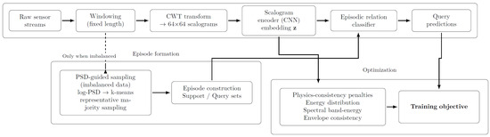
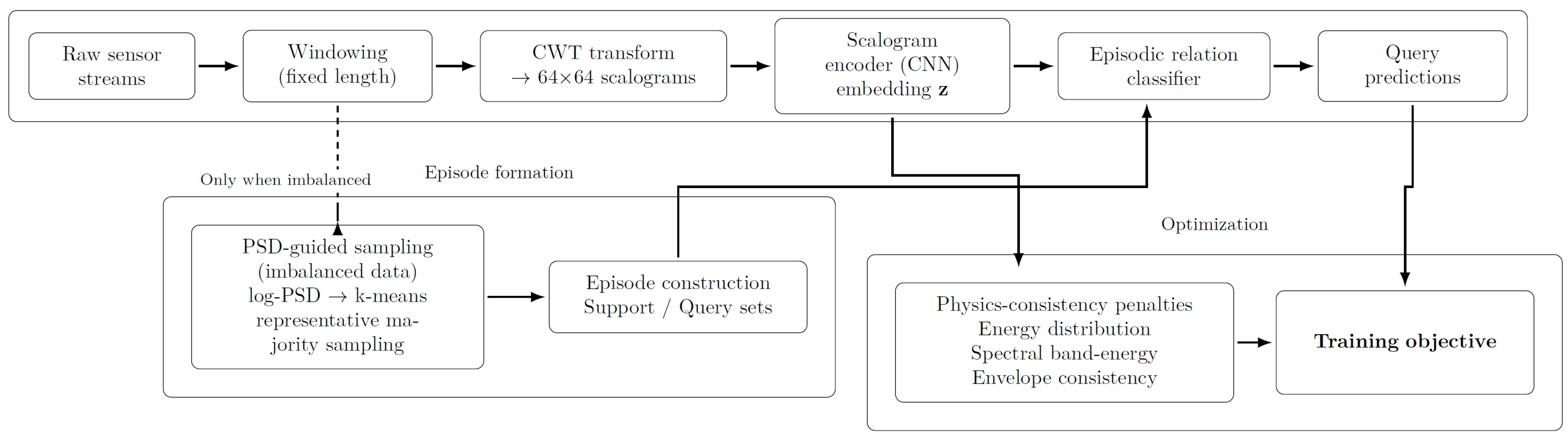
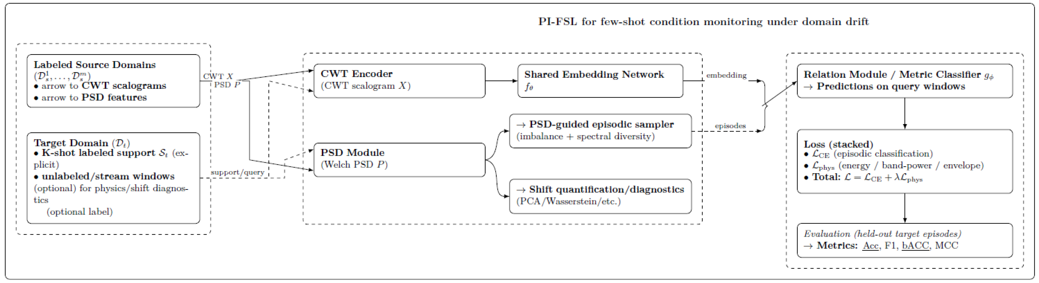
An overview of the proposed PI-FSL methodology is provided in Figure 1. The complete training procedure is summarized in Algorithm 1 and Figure 2. The implementation details are reported in Section 4.3.
| Algorithm 1. PI-FSL training with PSD-guided episodes and physics-informed regularization. |
| Input: source domains , target domain ; sampling rate ; window length (samples) and overlap ratio ; CWT settings; PSD/Welch settings; episode parameters ; number of episodes ; physics-loss weights and spectral bands . Output: trained embedding and relation module
|
Figure 1.
High-level PI-FSL methodology for cross-domain tool-wear monitoring. The pipeline includes (i) signal windowing and time–frequency transformation (CWT) to obtain scalograms, (ii) feature embedding and relation-based metric learning under episodic few-shot training, (iii) physics-consistency regularization (energy, spectral band ratio, and envelope terms) added to the episodic objective, and (iv) optional PSD-guided episodic sampling to mitigate severe class imbalances by diversifying healthy-class support samples.
Figure 2.
Overview of PI-FSL for few-shot condition monitoring under domain drift. CWT scalograms provide time–frequency features, PSD-based embeddings support imbalance-aware episodic sampling and shift diagnostics, and physics-consistency losses regularize episodic optimization.
4. Experimental Evaluation
This section describes the datasets, benchmark scenarios, preprocessing pipeline, implementation settings, and evaluation metrics used to assess PI-FSL. We report the results under explicit domain-drift scenarios, and we conducted swap and ablation studies to analyze the contribution of each component.
4.1. Signal Preprocessing and Windowing, and Leakage Control (Applied Across Datasets)
All datasets were processed using a consistent window-based pipeline. Raw signals were segmented into fixed-length windows with overlap. When multi-axis acceleration was available, channels were converted into a single magnitude signal. To reduce the impact of non-informative segments (e.g., idle or transient regions), we applied an activity gating strategy based on the amplitude and spectral content, and only retained windows that corresponded to stable operational regions.
For supervised labels, all windows extracted from a recording inherited the same recording-level label (e.g., healthy vs. worn, normal vs. fault). To avoid overlap leakage, we enforced support/query separation using disjoint sampling pools, and where applicable, we also used file-level splitting so that windows from the same recording did not appear in both the support and query sets within the same evaluation episode.
4.2. Datasets and Few-Shot Domain Adaptation Scenarios
We evaluated PI-FSL across one structured tool-wear benchmark and multiple bearing-fault datasets to assess its robustness under different types of domain drift. The evaluation included: (i) the Bosch tool-wear dataset for structured cross-domain benchmarking (E1–E4); (ii) the CWRU bearing dataset for cross-load swap evaluations; and (iii) a support suite of four cross-domain transfer scenarios spanning tool-wear and bearing diagnostics.
4.2.1. Tool-Wear Dataset: Bosch Benchmark Scenarios
The Bosch tool-wear dataset [26] was used to construct a structured cross-domain benchmark. Each domain was defined by a combination of the machine (M01/M02), operation (OP05/OP07), and time period, enabling explicit factor-level decomposition of the domain drift.
We defined four transfer scenarios:
- •
- E1 (cross-machine): same operation, different machine;
- •
- E2 (cross-operation): same machine, different operation;
- •
- E3 (combined machine–operation shift): both machine and operation differ;
- •
- E4 (multi-source to target): multiple source domains to a combined-shift target.
All source–target splits were fixed to ensure reproducibility. Table 1, Table 2 and Table 3 summarize the domain inventory, class imbalance statistics, and few-shot episodic configurations.
Table 1.
Bosch benchmark domain inventory (domains and periods used in E1–E4).
Table 2.
Bosch benchmark class imbalance by domain and period.
Table 3.
Cross-domain benchmark scenarios and splits (sources, targets, adaptation/evaluation).
4.2.2. Bearing Dataset: CWRU Swap Transfer Scenario
For the swap experiment, we used the Case Western Reserve University (CWRU), Cleveland, OH, USA, bearing dataset [27] (drive-end vibration) and constructed a binary task (normal vs. fault). We evaluated the cross-load transfer from Load 0 (source) to Load 2 (target) using fixed-length windows with overlap; support and query windows were sampled from disjoint pools to avoid overlap leakage. This experiment serves as a controlled portability check rather than a peak-performance benchmark for bearing diagnoses. The objective was to evaluate whether the same episodic framework can be reused across heterogeneous degradation mechanisms without architectural redesign.
4.2.3. Support-Suite Datasets and Unified Cross-Domain Protocol
To strengthen the external validity beyond the Bosch benchmark, we evaluated PI-FSL on a support suite of four cross-domain transfer scenarios spanning tool-wear and bearing diagnostics:
- Bosch cross-machine tool-wear transfer;
- HUST-CN frequency-shift transfer (20 Hz → 80 Hz), based on the Huazhong University of Science and Technology bearing dataset (Wuhan, China) [26];
- HUST-VN operating-condition shift (0 W → 200 W), based on the Hanoi University of Science and Technology bearing dataset (Hanoi, Vietnam) [28];
- PU bearing operating-condition transfer (N15M07F10 → F04), based on the Paderborn University bearing dataset (Paderborn, Germany) [25,29].
All scenarios were evaluated under a unified two-way five-shot protocol. We report the macro-F1 and balanced accuracy as the mean ± 95% confidence interval over repeated evaluation episodes.
4.2.4. Baselines Tied to Datasets
We compared PI-FSL against four representative few-shot baselines (matching networks, prototypical networks, relation networks, and MAML). All methods used the same input representation and episodic protocol per scenario to ensure comparability. In addition, we included a cross-dataset swap baseline where a bearing-oriented MAML pipeline was applied to the Bosch transfer setting to examine the transferability under a representation/task mismatch.
4.3. Implementation Details and Hyper-Parameters
4.3.1. Windowing and Overlap
Dataset-specific sampling rates and window sizes followed standard practice for each dataset. For Bosch, the signals were sampled at 2 kHz (Nyquist 1 kHz). We used two window configurations (1000 samples with 500 hop, and 512 samples with 256 hop), both with 50% overlap. For CWRU and the other datasets, the signals were sampled at 12 kHz, and we used 1024-sample windows with 50% overlap.
4.3.2. CWT Configuration
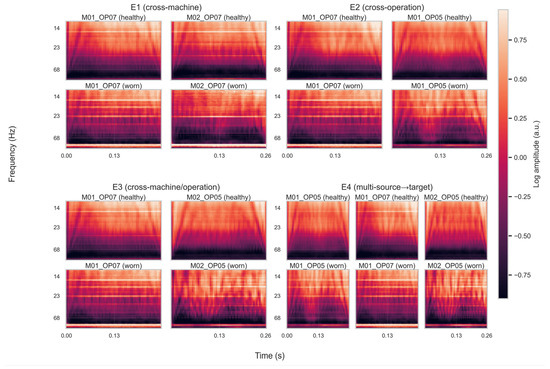
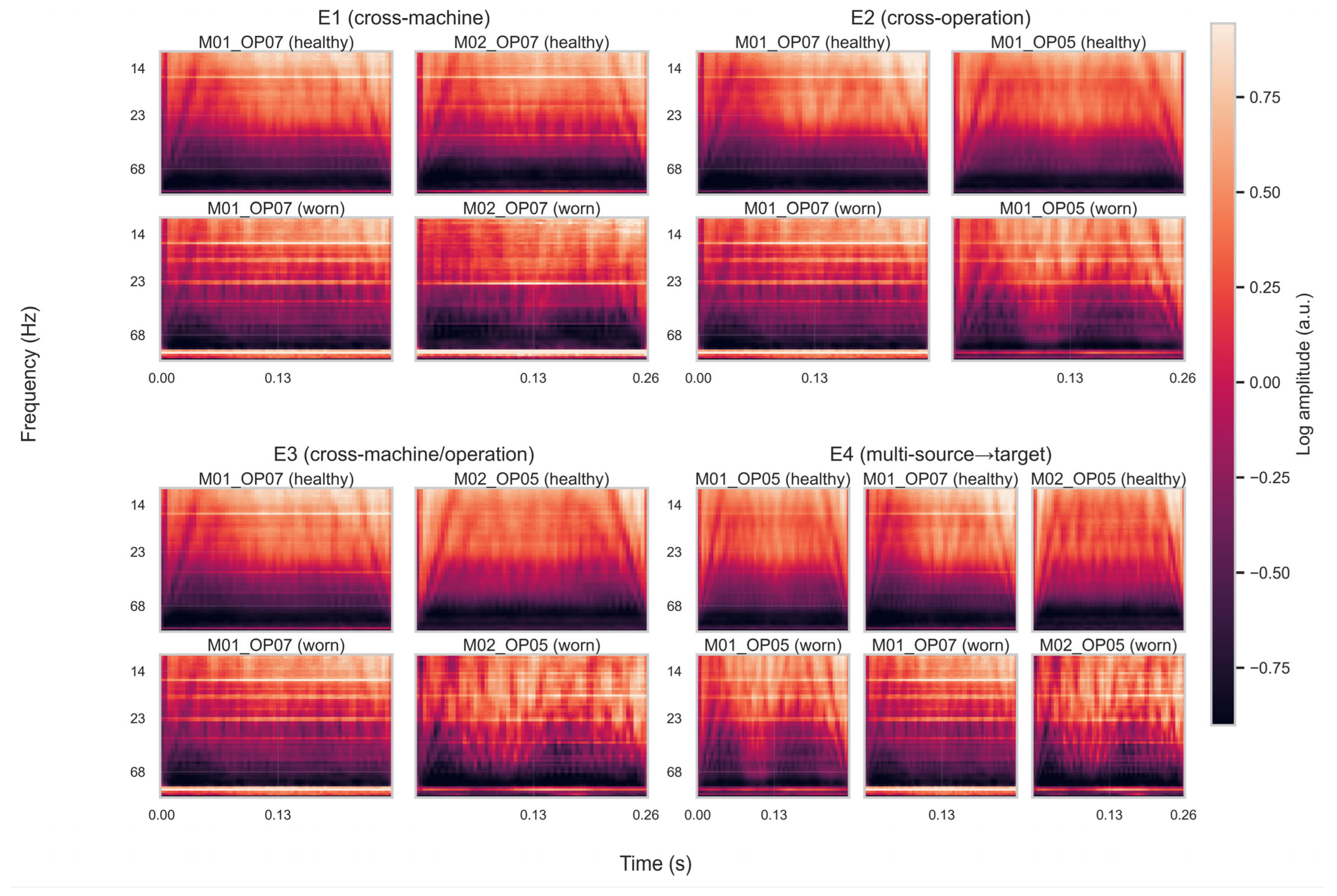
For each window, we computed a 2D scalogram using CWT (Morlet wavelet, 64 scales) [30]. Scalograms capture non-stationary spectral events that can be attenuated by purely Fourier-based summaries [31]. Other non-stationary decompositions (e.g., VMD) have also been used for tool-wear monitoring [32]. Representative mean scalograms are illustrated in Figure 3 for the Bosch dataset across domains and wear states.
Figure 3.
Mean CWT scalograms by domain and wear state for benchmark scenarios E1–E4, illustrating cross-domain variability in time–frequency patterns.
4.3.3. Physics Loss Configuration
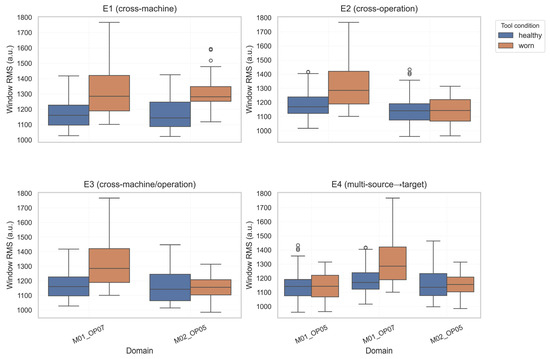
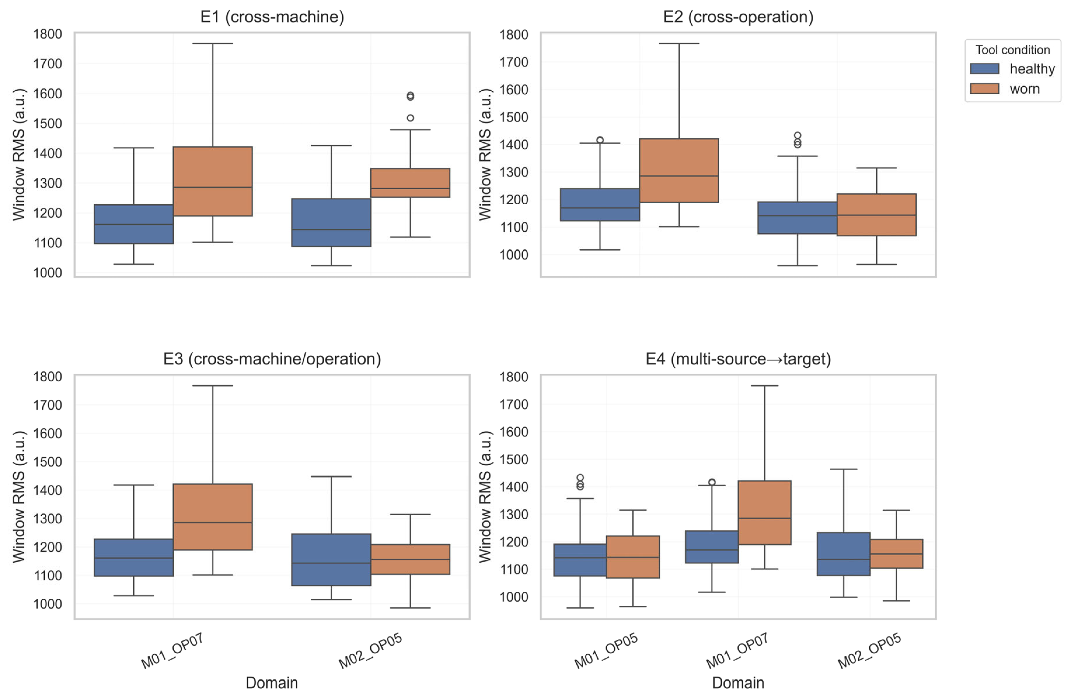
PI-FSL includes three physics-consistency terms: (i) the energy consistency, (ii) the band-power ratio consistency, and (iii) the envelope smoothness. Band-power ratios were computed using Welch PSD with fixed frequency bands; loss weights were treated as hyperparameters, and unless stated otherwise, we used (0.10, 0.10, 0.05) [33]. Figure 4 shows an example of the RMS distribution shifts that motivate energy consistency regularization for the Bosch dataset.
Figure 4.
Distribution shift in window RMS amplitude across domains for Bosch dataset: E3 (cross-machine/operation) and E4 (multi-source → target), motivating energy-consistency regularization.
Welch-based PSD features were used to compute the band energies and to construct PSD embedding for sampling. The PSD-guided sampling clustered majority-class windows in the PSD-embedding space using k-means, and representative windows were selected as the samples nearest to the cluster centroids. The number of clusters was set to with , capped so that , where is the number of majority-class windows. The physics-consistency loss was evaluated at every training episode under the default setting.
4.3.4. PSD Feature Configuration
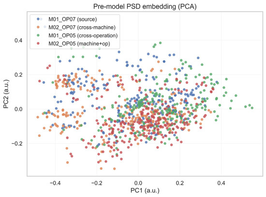
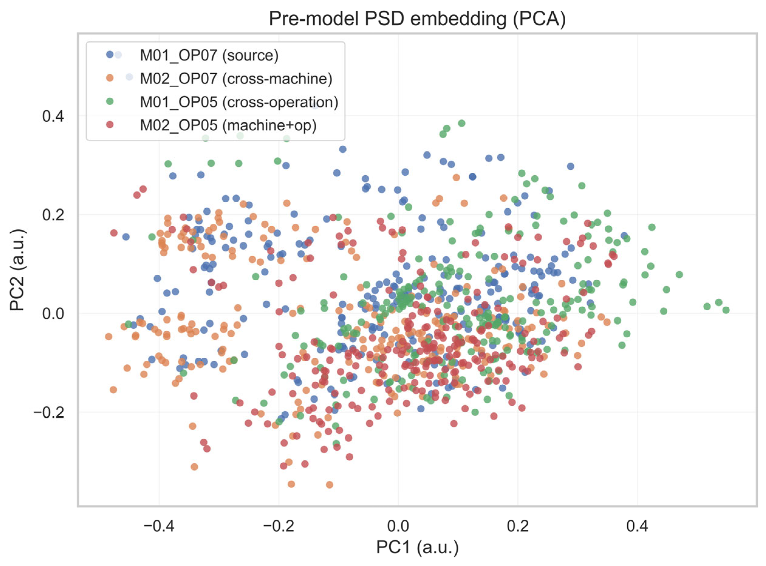
To address strong class imbalances without relying on synthetic oversampling, PI-FSL uses PSD-derived features to guide episodic sampling. Healthy windows are clustered in PSD-feature space (k-means), and representative healthy samples are drawn across clusters while retaining worn samples, producing episodes that are more balanced and spectrally diverse. Figure 5 shows an example of PSD for the Bosch dataset. It is obvious that PSD embeddings already separate domains before learning, motivating their use for episode construction and shift quantification.
Figure 5.
Pre-model PSD embedding (log-PSD + principal component analysis (PCA)) showing domain separation among Bosch machine–operation–period domains.
4.3.5. Episodic Training and Optimization
For the Bosch dataset benchmark scenarios, episodic training uses two-way classification with K = 1 and Q = 15 for 1200 training episodes and 200 validation episodes. A transfer fine-tuning stage then uses K = 5 support samples per class for 200 episodes. For the CWRU PI-FSL swap experiment, we used K = 3 and Q = 16, with 1000 training episodes and 200 evaluation episodes. In the Bosch transfer experiments, we report the results for K ∈ {1,5} to reflect both an extreme label-scarcity case (one-shot) and a small-support commissioning case (five-shot). We emphasized five-shot in the unified support suite because it provided a stable comparison point across datasets; K can be adjusted within the same episodic framework. For the remaining support-suite datasets, we used a unified two-way five-shot protocol to ensure a fair comparison across datasets. Unless stated otherwise, we set Q = 15 and used the same training and evaluation episode counts as the Bosch dataset benchmark. To reduce the computational overhead, the physics loss was evaluated every 10 episodes and used up to 1000 raw windows when required.
4.3.6. Reproducibility Details for PSD Sampling and Physics Losses
For PSD and band-energy features, Welch’s method was applied with a segment length of min(256, window length). The band energies were obtained by trapezoidal integration of the PSD over pre-defined frequency ranges. For PSD-guided sampling, majority-class windows were clustered in PSD-embedding space using k-means. When not specified, the number of clusters was set to with , capped so that ; in each cluster, the representative is the window closest to the centroid in Euclidean distance. For the spectral band-energy consistency term, the default bands were 0–75 Hz (low), 75–300 Hz (mid), and 300–1000 Hz (high), with the upper bound clipped to remain below the Nyquist frequency when applicable. The physics-consistency loss was evaluated at every training episode under the default setting.
4.4. Results and Discussion
4.4.1. Bosch Benchmark Performance
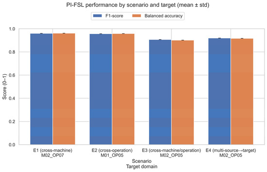
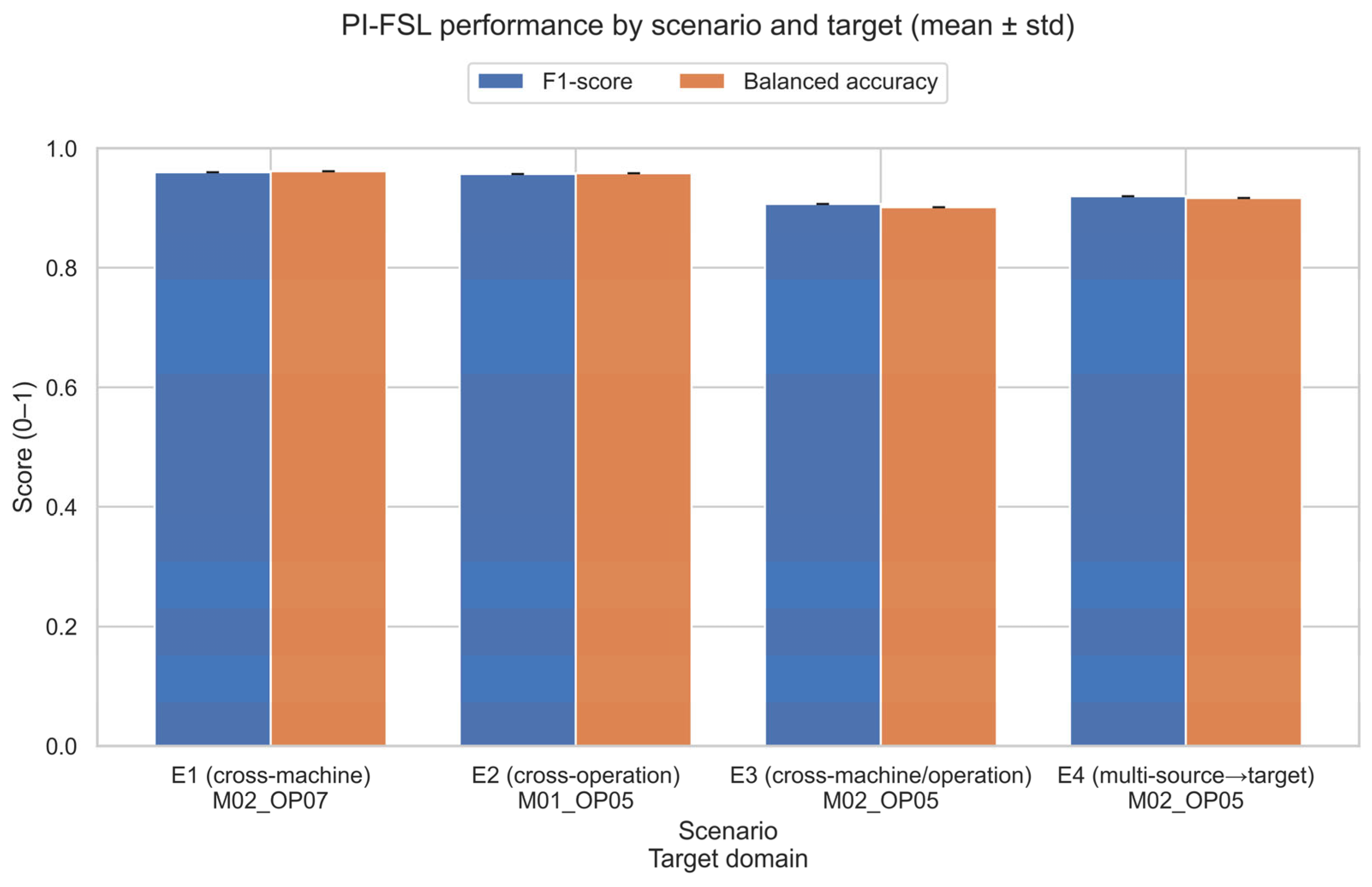
Table 4 summarizes the PI-FSL performance on the Bosch benchmark across the four transfer scenarios. In the cross-machine setting (E1: M01_OP07 → M02_OP07), PI-FSL achieved an F1 = 0.960 and a balanced accuracy = 0.961, with perfect precision (1.000) and a recall = 0.922. Cross-operation transfer (E2: M01_OP07 → M01_OP05) was similarly strong, reaching an F1 = 0.957 and a balanced accuracy = 0.958.
Table 4.
PI-FSL results on the Bosch benchmark (per-target metrics).
The performance decreased under the more challenging combined machine–operation shift (E3: M01_OP07 → M02_OP05), where F1 dropped to 0.907 and the balanced accuracy to 0.901. Compared to the cross-machine case (E1), this corresponds to an F1 reduction of 0.053. This reduction reflects the increased transfer difficulty when both machine characteristics and operating regimes change simultaneously.
Introducing multi-source training (E4: M01_OP05 and M01_OP07 → M02_OP05) improves the combined-shift result to F1 = 0.920 and a balanced accuracy = 0.917, yielding an F1 gain of 0.013 over the single-source setting. The improvement suggests that incorporating source diversity helps mitigate the compounded domain shift. A compact scenario-by-target visualization of the F1-score and balanced accuracy is provided in Figure 6.
Figure 6.
PI-FSL performance on Bosch benchmark targets by scenario and target domain (F1-score and balanced accuracy; point estimates aggregated over 200 evaluation episodes per target).
To contextualize these results, Table 5 reports the DG/DA baselines under the same Bosch domain splits. Deep CORAL achieved an F1 = 0.493 ± 0.014 (balanced accuracy = 0.517 ± 0.007) for E3 and an F1 = 0.541 ± 0.010 (balanced accuracy = 0.542 ± 0.011) for E4, substantially below PI-FSL under the same episodic protocol. DANN, evaluated non-episodically on E1, achieved an F1 = 0.957 and a balanced accuracy = 0.932, remaining below PI-FSL in the balanced accuracy. These comparisons indicate that episodic adaptation with integrated physics consistency provides a stronger robustness under the defined Bosch splits.
Table 5.
DG/DA baselines on the Bosch benchmark under the same domain splits as Table 4. Deep CORAL was evaluated in the same 2-way 5-shot episodic protocol and reported as the mean ± standard deviation over 5 random seeds (200 evaluation episodes per seed). DANN was evaluated on the full target set (non-episodic) and reported for a single run (seed 42).
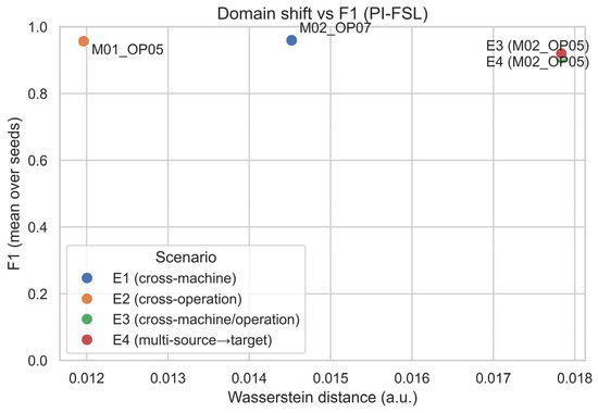
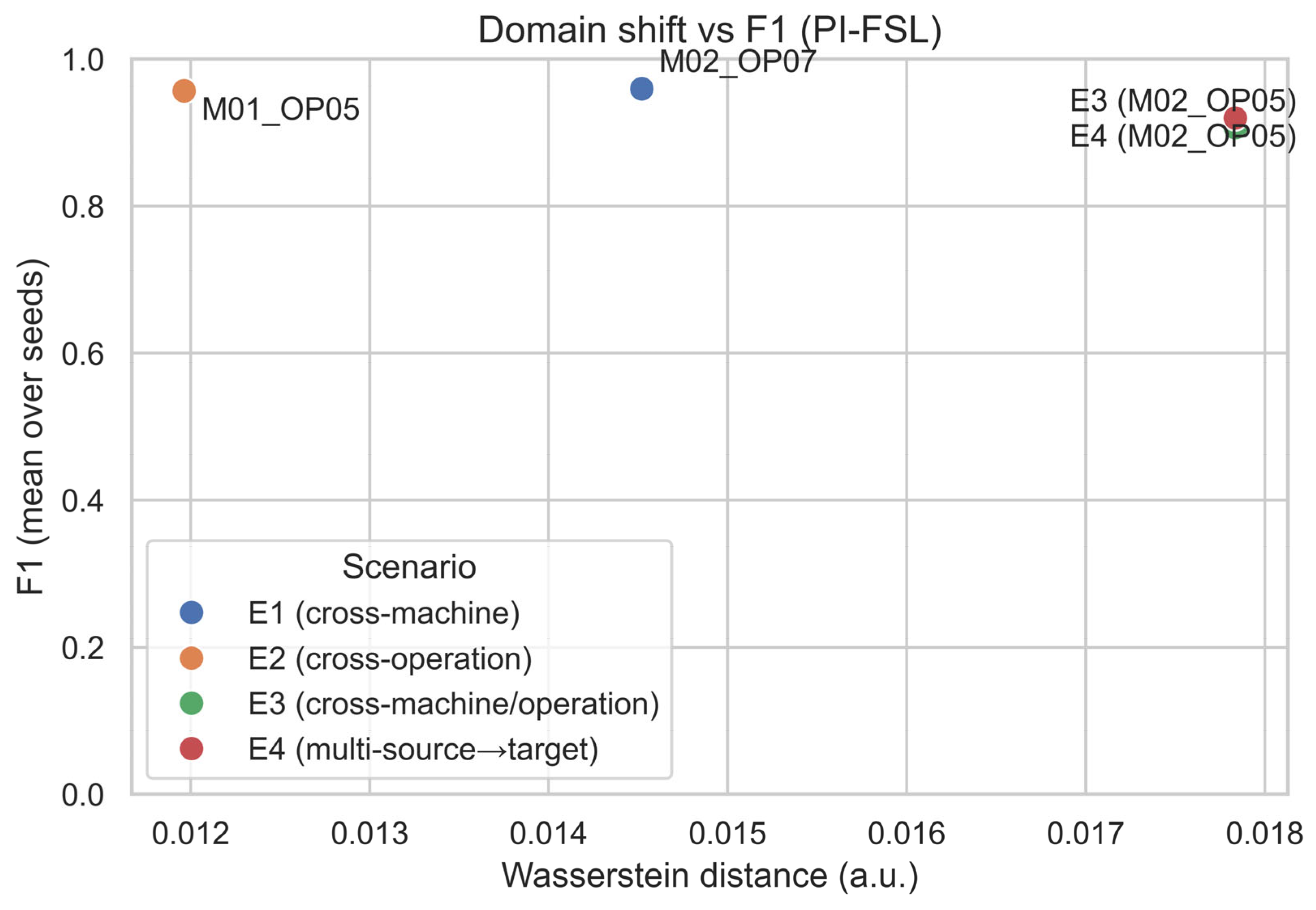
Because binary wear monitoring is highly imbalanced, we report the F1, balanced accuracy, and MCC alongside the accuracy, and we also report the precision/recall to expose asymmetric error modes; the confidence behavior was inspected via score distributions and threshold sensitivity [21]. The Bosch per-scenario metrics were taken from the exported run summary used for Table 4. Figure 7 relates these per-target F1 outcomes to the measured PSD-space domain shift, highlighting which transfer cases are intrinsically harder.
Figure 7.
Domain-shift sensitivity: PSD-space Wasserstein distance versus PI-FSL F1 across Bosch targets.
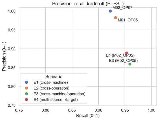
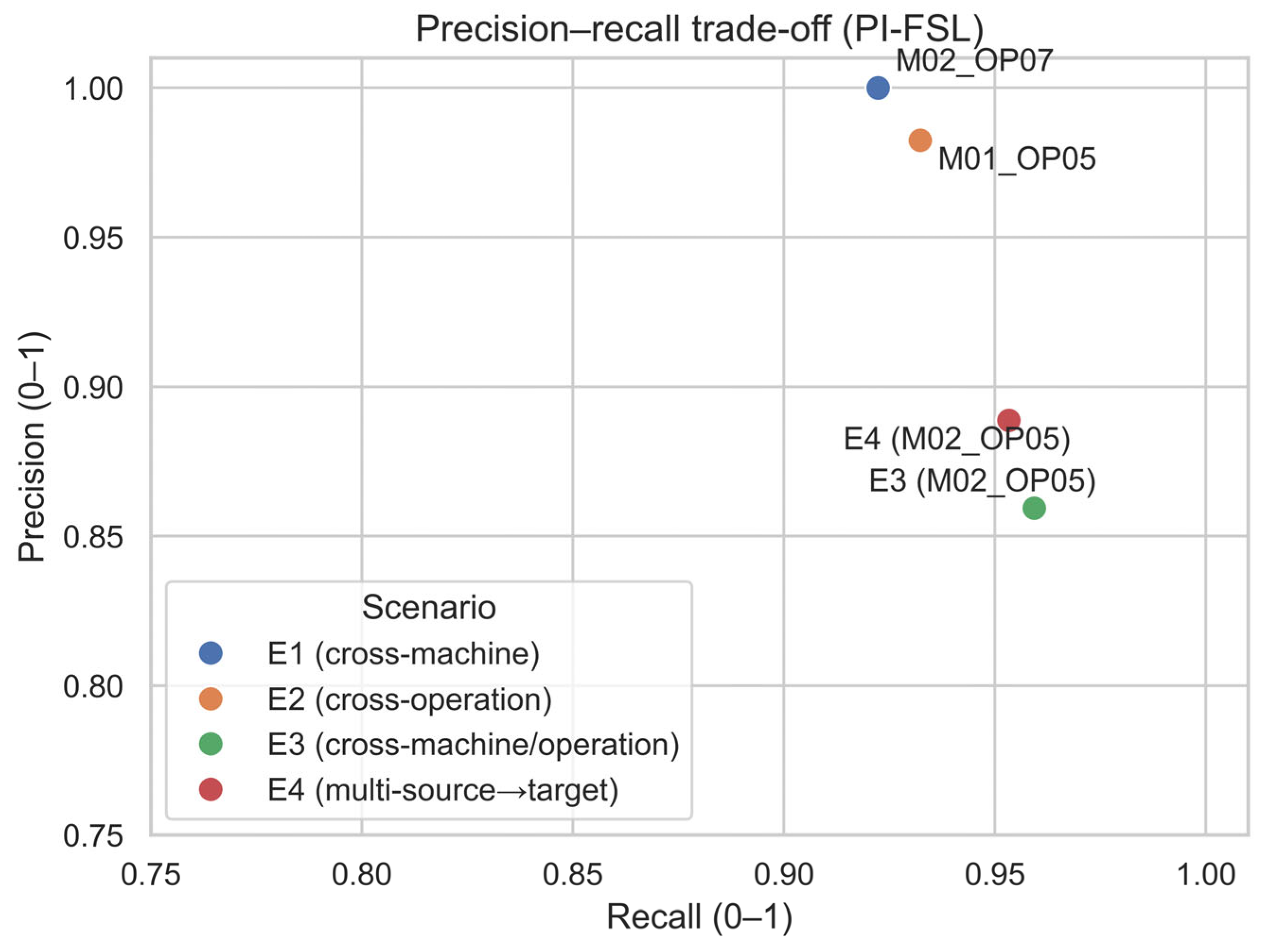
The metric breakdown revealed distinct error modes. For M02_OP07, the precision was 1.0 with a recall of 0.922, indicating that, when the model predicts worn, it is almost always correct, but it misses some worn windows (false negatives). For the combined-shift M02_OP05, the recall was high (0.959) while the precision decreased (0.859), suggesting that, in the hardest shift, the model tends to over-predict wear (more false positives) to avoid missing worn cases. This shift in the precision–recall balance is consistent with a more conservative decision boundary under a higher domain mismatch. In many industrial settings where missed wear is more costly than false alarms, this trade-off may be preferable; however, the decision threshold should be tuned to the deployment cost function and validated on held-out target periods [31]. The precision–recall trade-offs across Bosch targets are summarized in Figure 8.
Figure 8.
Precision–recall trade-off across Bosch targets (aggregated over 200 evaluation episodes per target), highlighting error-mode differences under combined shifts.
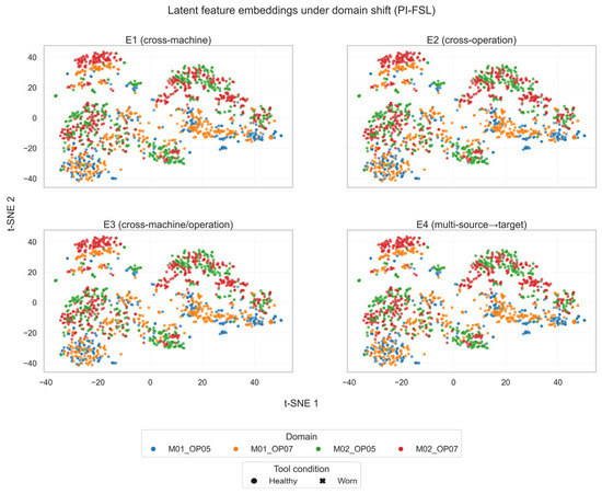
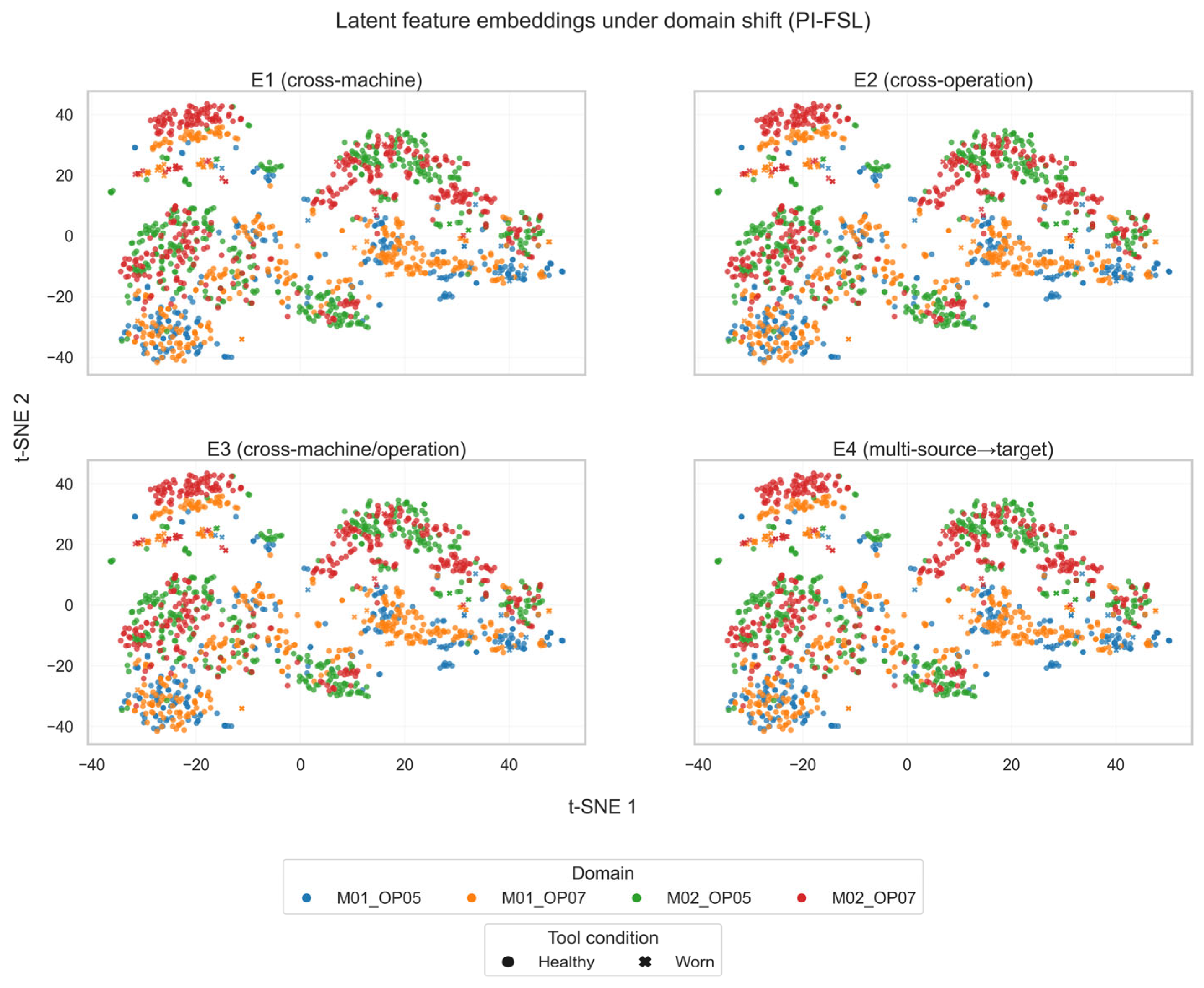
To further interpret this performance gap in feature space, Figure 9 visualizes the learned embeddings using t-SNE for the cross-machine (E1) and combined machine–operation (E3) scenarios. Under E1, the class clusters remained relatively well separated, despite the domain shift. In contrast, E3 exhibited substantially greater cross-domain overlap in the learned embedding space, consistent with the larger performance drop observed in Table 4. This visualization supports the interpretation that compounded drift increases class-boundary ambiguity rather than merely shifting global statistics.
Figure 9.
Learned feature embeddings under domain shift t-distributed stochastic neighbor embedding (t-SNE) for cross-machine and combined machine–operation targets.
4.4.2. Swap Study: Cross-Task Portability Under Matched Episodic Settings
While the Bosch benchmark evaluates structured domain shifts within a single monitoring problem, it does not assess cross-problem portability. We therefore conducted a controlled swap study to examine how the framework behaves when applied across heterogeneous degradation mechanisms. To assess the cross-task portability, we conducted a controlled swap study between the Bosch drilling-wear dataset and the CWRU bearing-fault dataset. The objective was to evaluate whether each pipeline can transfer under matched few-shot settings without redesigning the representation, preprocessing, or episodic task formulation. The results are summarized in Table 6.
Table 6.
Cross-dataset/method swap experiments (Bosch–CWRU).
We first evaluated whether PI-FSL, configured under the Bosch drilling episodic setting, can be directly applied to the CWRU bearing dataset without architectural modification. Using a binary normal-vs.-fault configuration (two-way, K = 3, Q = 16), PI-FSL achieved a near-perfect performance (accuracy = 1.000, F1 = 1.000, balanced accuracy = 1.000, MCC = 1.000). The experimental results showed that the same PI-FSL pipeline can be reused across datasets without redesigning the representation, preprocessing, or training strategy.
We next examined an MAML configuration reported to perform well on CWRU bearing diagnoses (10-way five-shot with STFT), achieving a mean accuracy = 0.984 under its native setting. By applying a comparable few-shot configuration to the Bosch drilling cross-machine scenario (M01_OP07 → M02_OP07, two-way five-shot, 15-query), the MAML pipeline achieved a mean episodic accuracy = 0.798. The degradation reflects structural differences between bearing faults (discrete fault-frequency signatures and categorical labels) and drilling wear (gradual time–frequency evolution and progression-based semantics).
Overall, the swap study indicates that PI-FSL is more tolerant to structural differences across degradation mechanisms. Its multi-resolution CWT representation, relation-based episodic comparison, and physics-consistency regularization together improve the robustness under cross-problem transfer without requiring architectural changes.
4.4.3. Support-Suite Results Under Cross-Domain Datasets
In this sub-section, we extend the evaluation to a support suite spanning four cross-domain datasets to assess the robustness under a unified two-way five-shot protocol. Table 7 and Table 8 summarize the macro-F1 and balanced accuracy (mean ±95% CI) across the four scenarios. PI-FSL achieved the best performance in all cases. The performance margin was scenario-dependent: the gains were modest on the easier HUST-CN and HUST-VN frequency-shift transfers, where several methods approached a near-ceiling performance, but they became more pronounced on Bosch drilling and particularly on the PU bearing transfer, which represents the most challenging setting in the suite.
Table 7.
Support-suite macro-F1 (mean ± 95% confidence interval (CI)) across four cross-domain datasets. Aggregated over 200 evaluation episodes per method–scenario.
Table 8.
Support-suite balanced accuracy (mean ±95% CI) across four cross-domain datasets. Aggregated over 200 evaluation episodes per method–scenario.
When averaged across scenarios, PI-FSL attained the highest macro-F1 and balanced accuracy, indicating an improved robustness beyond the original tool-wear benchmark. The lower across-method averages observed on PU bearing further confirm its higher intrinsic difficulty under the selected transfer configuration.
4.4.4. Ablation and Interpretation
To isolate the contribution of each component, we conducted structured ablations on the Bosch benchmark and extended selected analyses across datasets. All the results were aggregated over repeated trials as specified in the corresponding tables. The ablation study was organized into three parts: (i) the relative contribution of episodic fine-tuning and physics-consistency regularization, (ii) imbalance-handling strategies, and (iii) a component-wise analysis of the physics terms.
We first examined the importance of episodic fine-tuning and physics regularization on the Bosch support-suite setting; the results are shown in Table 9. Removing few-shot fine-tuning reduced the macro-F1 from 0.997 to 0.736, confirming that episodic adaptation is the primary alignment mechanism under domain shifts. In contrast, removing physics regularization reduced the macro-F1 from 0.997 to 0.991, indicating a smaller, but consistent, stabilizing effect. These results suggest that physics losses act as soft regularizers, while few-shot adaptation remains essential for effective transfer.
Table 9.
Ablation on the Bosch support-suite setting (mean ±95% CI). Aggregated over 200 evaluation episodes per ablation setting.
Table 10 compares imbalance-handling strategies on Bosch E3 (M01_OP07 → M02_OP05, two-way one-shot). All three strategies performed comparably: no balancing achieved 0.933 ± 0.052, random class-balanced sampling achieved 0.935 ± 0.052, and PSD-guided sampling achieved 0.937 ± 0.067. The slight improvement with PSD-guided selection suggests that diversity-aware episode construction can provide incremental benefits, though imbalance handling does not dominate the performance in this relatively moderate setting.
Table 10.
Episode construction under class imbalance on Bosch E3 (M01_OP07 → M02_OP05, 2-way 1-shot). Results are mean ± std over 5 seeds (200 evaluation episodes/seed).
The cross-dataset imbalance analysis in Table 11 provides a clearer picture. On Bosch, the performance remained strong across balance modes, with only a modest gain from PSD-guided sampling (macro-F1: 0.992 ± 0.022), indicating limited sensitivity to the imbalance strategy. On PU, however, PSD-guided sampling substantially improved the macro-F1 to 0.663 ± 0.015, compared to 0.459 ± 0.085 (none) and 0.458 ± 0.087 (random). This demonstrates that diversity-aware episode construction becomes particularly important in more challenging cross-domain scenarios.
Table 11.
Imbalance-handling ablation across Bosch and PU under the episodic protocol. All results use 2-way 5-shot episodic training with 200 training episodes and 200 evaluation episodes per run, with scalogram_64 × 64 inputs. Values are mean ± std over 3 seeds (seeds 1–3). “PSD-guided” denotes PSD-guided episodic selection; “random” denotes random class-balanced episodic sampling.
We next examined the contribution of individual physics terms. On Bosch E1 in Table 12 (two-way one-shot), removing physics regularization or isolating individual components (energy-only, spectral-only, envelope-only) yielded closely clustered macro-F1 values (0.911–0.914), confirming that no single term independently drives performance. Instead, physics constraints act collectively as mild stabilizers.
Table 12.
Component-wise physics regularization ablations on Bosch E1 (M01_OP07 → M03_OP07, 2-way 1-shot, PSD sampling off). Results are mean ± std over 5 seeds (200 evaluation episodes/seed).
Finally, Table 13 extends this analysis under a unified episodic protocol across Bosch and PU. On Bosch, the full model achieved a higher macro-F1 (0.993 ± 0.021), while removing or isolating physics terms yielded a lower, but similar, performance among ablations (0.949–0.953), suggesting that the physics terms provide a clear gain in this setting. On PU, however, removing physics regularization significantly degraded the performance from 0.663 ± 0.015 to 0.474 ± 0.089, with similar drops observed for individual terms (0.465–0.472). This indicates that physics-consistency regularization provides meaningful robustness under more severe domain shifts, even though it does not function as a standalone feature extractor.
Overall, these ablations confirm that episodic fine-tuning is the dominant adaptation mechanism, while physics regularization and diversity-aware episode construction contribute incremental, but scenario-dependent, robustness.
Table 13.
Physics-term ablation across Bosch and PU under the episodic protocol. All results use 2-way 5-shot episodic training with 200 training episodes and 200 evaluation episodes per run, with scalogram_64 × 64 inputs. Values are mean ± std over 3 seeds (seeds 1–3). Metrics are macro-F1 and balanced accuracy aggregated over evaluation episodes.
5. Conclusions
This work presents PI-FSL, an integrated episodic learning framework that embeds physics-consistency regularization within few-shot domain adaptations for condition monitoring under domain drift. The framework combines CWT-based time–frequency encoding, relation-based episodic classification, soft physics constraints at representation and signal levels, and imbalance-aware episode construction into a unified, deployment-oriented pipeline.
We evaluated PI-FSL across multiple cross-domain condition-monitoring datasets, including a scenario-structured tool-wear benchmark and several bearing-fault transfer settings. The results showed that episodic adaptation enables effective cross-domain alignment under limited target labels, while physics-consistency regularization provides a structured inductive bias that enhances the robustness, particularly under compounded machine–operation shifts. Multi-source training further improves the stability when multiple drift factors are present.
Under a unified few-shot protocol spanning tool-wear and bearing diagnostics, PI-FSL achieved a consistently competitive performance and ranked first in the macro-F1 and balanced accuracy across the evaluated scenarios. These findings support PI-FSL as a transferable engineering framework for robust few-shot adaptation across heterogeneous industrial monitoring tasks.
Future work will explore adaptive weighting of physics-consistency terms, extension to multi-level wear severity and regression settings (e.g., RUL), and evaluation under additional deployment drift factors such as sensor placement variation and sampling-rate mismatch.
Author Contributions
Conceptualization, J.W., K.P.Y., M.Y.H.L. and N.C.N.D.; Methodology, J.W., K.P.Y. and N.C.N.D.; Software, J.W.; Validation, J.W.; Formal analysis, J.W.; Investigation, J.W.; Resources, J.W., H.Y.N. and W.W.; Data curation, J.W.; Writing—original draft, J.W.; Writing—review & editing, J.W., K.P.Y., M.Y.H.L., N.C.N.D., H.Y.N. and W.W.; Visualization, J.W.; Supervision, K.P.Y., M.Y.H.L., C.X., N.C.N.D., H.Y.N. and W.W.; Project administration, J.W., C.X., H.Y.N. and W.W.; Funding acquisition, C.X., H.Y.N. and W.W. All authors have read and agreed to the published version of the manuscript.
Funding
This research was partially supported by the Ministry of Trade and Industry (MTI) and A*STAR under the Sectoral AI Centre of Excellence for Manufacturing Programme (award No. W24MFMF001), and the RIE2025 Manufacturing, Trade and Connectivity (MTC) Industry Alignment Fund—Pre-Positioning (IAF-PP) (award No. M23L4a0001).
Institutional Review Board Statement
Not applicable. This study did not involve humans or animals; therefore, ethical review and approval were not required.
Informed Consent Statement
Not applicable.
Data Availability Statement
The datasets analyzed in this study are publicly available from the repositories cited in the manuscript. The Bosch CNC machining dataset is available from the UCI Machine Learning Repository, University of California, Irvine, Irvine, CA, USA, and the Bosch Research GitHub repository. The Case Western Reserve University (CWRU) bearing dataset is available from the Bearing Data Center, Case Western Reserve University, Cleveland, OH, USA. The Paderborn University bearing dataset (PU) is available from Paderborn University, Paderborn, Germany, via the TIB dataset service (DOI: 10.57702/h4gb3nzj). The HUST bearing dataset—Vietnam is associated with Hanoi University of Science and Technology, Hanoi, Vietnam, and is available from Mendeley Data (DOI: 10.17632/cbv7jyx4p9.3). The HUST bearing dataset—China is associated with Huazhong University of Science and Technology, Wuhan, China, and is available from a public GitHub repository. The code used for preprocessing, model training, and evaluation is available from the public GitHub repository “PI-FSL-MDPI-Technologies”.
Acknowledgments
The authors would like to thank colleagues and collaborators for their helpful discussions and feedback that improved the presentation of this work.
Conflicts of Interest
The authors declare no conflicts of interest.
Abbreviations
The following abbreviations are used in this manuscript:
| BAL ACC | Balanced accuracy |
| CI | Confidence interval |
| CNC | Computer numerical control |
| CWT | Continuous wavelet transform |
| CWRU | Case Western Reserve University |
| FFT | Fast Fourier transform |
| FSL | Few-shot learning |
| F1 | F1-score |
| HUST | Hanoi University of Science and Technology |
| HUST bearing | Huazhong University of Science and Technology bearing dataset |
| MAML | Model-agnostic meta-learning |
| MCC | Matthews correlation coefficient |
| PdM | Predictive maintenance |
| PI-FSL | Physics-informed few-shot learning |
| PSD | Power spectral density |
| PU | Paderborn University bearing dataset |
| PQM | Process quality monitoring |
| RMS | Root mean square |
| STFT | Short-time Fourier transform |
References
- Wan, J.; Yar, K.P.; Du, C.; Low, M.Y.H. Sensor Data Analytics for Tool Condition Anomaly Detection with Machine Learning Techniques. In Proceedings of the 2023 5th International Electronics Communication Conference, Osaka, Japan, 21–23 July 2023; ACM: New York, NY, USA, 2023; pp. 38–45. [Google Scholar]
- Li, S.; Li, M.; Gao, Y. Deep Learning Tool Wear State Identification Method Based on Cutting Force Signal. Sensors 2025, 25, 662. [Google Scholar] [CrossRef] [Scilit] [PubMed]
- Papacharalampopoulos, A.; Alexopoulos, K.; Catti, P.; Stavropoulos, P.; Chryssolouris, G. Learning More with Less Data in Manufacturing: The Case of Turning Tool Wear Assessment through Active and Transfer Learning. Processes 2024, 12, 1262. [Google Scholar] [CrossRef] [Scilit]
- Zhang, W.; Li, C.; Peng, G.; Chen, Y.; Zhang, Z. A Deep Convolutional Neural Network with New Training Methods for Bearing Fault Diagnosis under Noisy Environment and Different Working Load. Mech. Syst. Signal Process. 2018, 100, 439–453. [Google Scholar] [CrossRef] [Scilit]
- Wang, D.; Liu, Q.; Wu, D.; Wang, L. Meta Domain Generalization for Smart Manufacturing: Tool Wear Prediction with Small Data. J. Manuf. Syst. 2022, 62, 441–449. [Google Scholar] [CrossRef] [Scilit]
- Liu, C.; Li, Y.; Li, J.; Hua, J. A Meta-Invariant Feature Space Method for Accurate Tool Wear Prediction under Cross Conditions. IEEE Trans. Ind. Inform. 2022, 18, 922–931. [Google Scholar] [CrossRef] [Scilit]
- Mo, X.; Hu, X.; Sun, A.; Zhang, Y. A Meta-Learning Method for Smart Manufacturing: Tool Wear Prediction Using Hybrid Information under Various Operating Conditions. Robot. Comput. Integr. Manuf. 2025, 91, 102846. [Google Scholar] [CrossRef] [Scilit]
- Li, W.; Fu, H.; Zhuo, Y.; Liu, C.; Jin, H. Semi-Supervised Multi-Source Meta-Domain Generalization Method for Tool Wear State Prediction under Varying Cutting Conditions. J. Manuf. Syst. 2023, 71, 323–341. [Google Scholar] [CrossRef] [Scilit]
- Shao, J.; Fang, D.; Huang, Z.; Zheng, Z.; Zhu, J. Multi-Source Feature Augmentation Adversarial Domain Generalization Method for Tool Wear Condition Monitoring on Unseen Machine Tools. J. Intell. Manuf. 2025. [Google Scholar] [CrossRef] [Scilit]
- Cai, Z.; Li, W.; Song, J.; Jin, H.; Fu, H. Tool Wear State Identification Method with Variable Cutting Parameters Based on Multi-Source Unsupervised Domain Adaptation. Sensors 2025, 25, 1742. [Google Scholar] [CrossRef] [Scilit] [PubMed]
- Zhao, C.; Zio, E.; Shen, W. Domain Generalization for Cross-Domain Fault Diagnosis: An Application-Oriented Perspective and a Benchmark Study. Reliab. Eng. Syst. Saf. 2024, 245, 109964. [Google Scholar] [CrossRef] [Scilit]
- Hou, W.; Guo, H.; Luo, L.; Jin, M. Tool Wear Prediction Based on Domain Adversarial Adaptation and Channel Attention Multiscale Convolutional Long Short-Term Memory Network. J. Manuf. Process. 2022, 84, 1339–1361. [Google Scholar] [CrossRef] [Scilit]
- Zhu, Y.; Zi, Y.; Xu, J.; Li, J. An Unsupervised Dual-Regression Domain Adversarial Adaption Network for Tool Wear Prediction in Multi-Working Conditions. Measurement 2022, 200, 111644. [Google Scholar] [CrossRef] [Scilit]
- Kim, G.; Yang, S.M.; Kim, S.; Kim, D.Y.; Choi, J.G.; Park, H.W.; Lim, S. A Multi-Domain Mixture Density Network for Tool Wear Prediction under Multiple Machining Conditions. Int. J. Prod. Res. 2023. [Google Scholar] [CrossRef] [Scilit]
- Qiang, B.; Shi, K.; Ren, J.; Shi, Y. Multi-Source Online Transfer Learning Based on Hybrid Physics-Data Model for Cross-Condition Tool Health Monitoring. J. Manuf. Syst. 2024, 77, 1–17. [Google Scholar] [CrossRef] [Scilit]
- Kim, G.; Yang, S.M.; Jeon, S.; Park, S.; Choi, J.G.; Park, H.W.; Lim, S. Robust Tool Wear Prediction under Novel Operating Conditions via Physics-Guided Unsupervised Domain Adaptation. Adv. Eng. Inform. 2026, 69, 103883. [Google Scholar] [CrossRef] [Scilit]
- Wang, Z.; Lu, Y.; Deng, K.; Liang, J.; Gao, D. Physics-Informed Self-Supervised Learning for Tool Wear Monitoring Leveraging Signal and Degradation Features under Limited Labels. Adv. Eng. Inform. 2025, 67, 103503. [Google Scholar] [CrossRef] [Scilit]
- Zhang, H.; Jiang, S.; Gao, D.; Sun, Y.; Bai, W. A Review of Physics-Based, Data-Driven, and Hybrid Models for Tool Wear Monitoring. Machines 2024, 12, 833. [Google Scholar] [CrossRef] [Scilit]
- Zhang, S.; Ye, F.; Wang, B.; Habetler, T.G. Few-Shot Bearing Fault Diagnosis Based on Model-Agnostic Meta-Learning. IEEE Trans. Ind. Appl. 2021, 57, 4754–4764. [Google Scholar] [CrossRef] [Scilit]
- Kim, J.; Kim, J.; Lee, H.U.; Choi, O.; Kim, S. UnderFSL: Boundary-Preserving Undersampling with Few-Shot Relation Networks for Cross-Machine CNC Fault Diagnosis. Electronics 2025, 14, 3699. [Google Scholar] [CrossRef] [Scilit]
- Wan, J.; Yar, K.P.; Hean Low, M.Y.; Du, C. Comparing Traditional Machine Learning and Deep Learning Methods for Imbalanced Vibration Signal-Based Tool Condition Monitoring. In Proceedings of the 2025 7th International Conference on Industrial Artificial Intelligence (IAI), Shenyang, China, 21–24 August 2025; IEEE: New York, NY, USA, 2025; pp. 1–6. [Google Scholar]
- Montesuma, E.F.; Mboula, F.N.; Souloumiac, A. Recent Advances in Optimal Transport for Machine Learning. IEEE Trans. Pattern Anal. Mach. Intell. 2025, 47, 1161–1180. [Google Scholar] [CrossRef] [Scilit]
- Sung, F.; Zhang, L.; Xiang, T.; Torr, P.H.S.; Hospedales, T.M. Learning to Compare: Relation Network for Few-Shot Learning. In Proceedings of the 2018 IEEE/CVF Conference on Computer Vision and Pattern Recognition; IEEE: New York, NY, USA, 2018. [Google Scholar]
- Cohen, R.; Bachar, L.; Matania, O.; Bortman, J. Few-Shot Learning for Estimating Gear Wear Severity towards Digital Twinning. Eng. Fail. Anal. 2025, 170, 109330. [Google Scholar] [CrossRef] [Scilit]
- Lessmeier, C.; Kuria Kimotho, J.; Zimmer, D.; Sextro, W. Condition Monitoring of Bearing Damage in Electromechanical Drive Systems by Using Motor Current Signals of Electric Motors: A Benchmark Data Set for Data-Driven Classification. In Proceedings of the European Conference of the PHM Society 2016, Bilbao, Spain, 5–8 July 2016. [Google Scholar]
- Tnani, M.A.; Feil, M.; Diepold, K. Smart Data Collection System for Brownfield CNC Milling Machines: A New Benchmark Dataset for Data-Driven Machine Monitoring. In Proceedings of the Procedia CIRP; Elsevier: Amsterdam, The Netherlands, 2022; Volume 107, pp. 131–136. [Google Scholar]
- Hendriks, J.; Dumond, P.; Knox, D.A. Towards Better Benchmarking Using the CWRU Bearing Fault Dataset. Mech. Syst. Signal Process. 2022, 169, 108732. [Google Scholar] [CrossRef] [Scilit]
- Thuan, N.D.; Hong, H.S. HUST Bearing: A Practical Dataset for Ball Bearing Fault Diagnosis. BMC Res. Notes 2023, 16, 138. [Google Scholar] [CrossRef] [Scilit]
- Lessmeier, C.; Kimotho, J.K.; Zimmer, D.; Sextro, W. Dataset: Paderborn University Bearing Dataset. Available online: https://mb.uni-paderborn.de/kat/forschung/bearing-datacenter/data-sets-and-download (accessed on 2 March 2026).
- Zhang, Y.; Qi, X.; Wang, T.; He, Y. Tool Wear Condition Monitoring Method Based on Deep Learning with Force Signals. Sensors 2023, 23, 4595. [Google Scholar] [CrossRef] [Scilit]
- Torrence, C.; Compo, G.P. A Practical Guide to Wavelet Analysis. Bull. Am. Meteorol. Soc. 1998, 79, 61–78. [Google Scholar] [CrossRef] [Scilit]
- Wang, K.; Wang, A.; Wu, L. Research on Tool Wear Monitoring Technology Based on Variational Mode Decomposition and Back Propagation Neural Network Model. Sensors 2024, 24, 8107. [Google Scholar] [CrossRef] [Scilit]
- Welch, P.D. The Use of Fast Fourier Transform for the Estimation of Power Spectra: A Method Based on Time Averaging Over Short, Modified Periodograms. IEEE Trans. Audio Electroacoust. 1967, 15, 70–73. [Google Scholar] [CrossRef] [Scilit]
- Snell, J.; Swersky, K.; Zemel, T.R. Prototypical Networks for Few-Shot Learning. arXiv 2017, arXiv:1703.05175. [Google Scholar]
- Vinyals, O.; Blundell, C.; Lillicrap, T.; Kavukcuoglu, K.; Wierstra, D. Matching Networks for One Shot Learning. arXiv 2017, arXiv:1606.04080. [Google Scholar]
- Finn, C.; Abbeel, P.; Levine, S. Model-Agnostic Meta-Learning for Fast Adaptation of Deep Networks. arXiv 2017, arXiv:1703.03400. [Google Scholar]

Disclaimer/Publisher’s Note: The statements, opinions and data contained in all publications are solely those of the individual author(s) and contributor(s) and not of MDPI and/or the editor(s). MDPI and/or the editor(s) disclaim responsibility for any injury to people or property resulting from any ideas, methods, instructions or products referred to in the content. |
© 2026 by the authors. Licensee MDPI, Basel, Switzerland. This article is an open access article distributed under the terms and conditions of the Creative Commons Attribution (CC BY) license.