


Abstract
Finite-element analysis (FEA) is a widely used computational method for predicting the biomechanical response of implant-supported prostheses, but its computational cost limits its use in large-scale parametric exploration or chairside decision support. This study evaluated whether supervised machine learning models trained on finite-element simulations can act as accurate, near-instantaneous surrogates, whether their predictions are driven by physically plausible input variables, and whether their residual error is small enough to preserve the verdict of a downstream, illustrative design-screening protocol. A finite-element dataset was generated for 100 independently meshed and solved parent configurations of a fixed, four-implant (“All-on-4”-type) implant-supported prosthesis, varying seven geometry-level input variables (bone quality, bar material, implant diameter and length, implant tilt angle, cantilever length, and occlusal load angle) using a custom three-dimensional finite-element solver implemented in Python; each parent solution was then linearly scaled to 71 occlusal-load magnitudes, yielding a 7100-row modeling dataset with four biomechanical outputs per row: 95th-percentile (P95) cortical bone von Mises stress, P95 trabecular bone von Mises stress, maximum prosthesis displacement, and P95 bone principal strain. All 100 parent simulations converged and passed internal quality-control checks on solver residuals and force-balance equilibrium. Because rows sharing a parent geometry are not statistically independent, all partitioning and cross-validation were performed at the geometry level: 20 geometries (1420 rows) were held out a priori as a fixed test set, and the remaining 80 geometries (5680 rows) formed a development pool on which Random Forest, XGBoost, and support-vector regression (SVR) models were compared using grouped cross-validation GroupKFold keyed on parent geometry, 5 folds × 5 repeats, 25 matched folds), with model selection performed independently for each output based on the lowest mean cross-validated RMSE. This yielded a different winning model per output rather than a single globally best algorithm: target-scaled SVR for both P95 cortical stress ( MPa) and P95 trabecular stress ( MPa), Random Forest for maximum displacement ( mm), and XGBoost for P95 principal strain ( ). Friedman and Holm-corrected pairwise Wilcoxon signed-rank tests corroborated that this ranking was consistent across resampled folds, but the more practically relevant evidence is the magnitude of the differences themselves, which is reported primarily as percentage RMSE reduction and matched-pairs rank-biserial effect size: 14.5% (cortical stress), 1.5% (trabecular stress, a practically negligible difference), 9.4% (displacement), and 15.0% (principal strain). Each selected model was refit on the full 80-geometry development pool and evaluated once, without further tuning, on the fixed 20-geometry (1420-row) test set. On this held-out test set, the selected models achieved coefficients of determination () of 0.985 (95% bootstrap CI 0.976 to 0.993) for cortical stress, 0.968 (0.946 to 0.982) for trabecular stress, 0.986 (0.977 to 0.993) for maximum displacement, and 0.931 (0.883 to 0.980) for principal strain, with mean absolute percentage errors between 7.99% and 14.88%. SHAP (SHapley Additive exPlanations) analysis of the actual selected model for each output (TreeExplainer for Random Forest and XGBoost; KernelExplainer for SVR) showed that occlusal load magnitude was the dominant driver of both stress outputs and of principal strain (39 to 45% of attributed importance), bone quality contributed materially to trabecular stress and strain (19% and 31%, respectively), and bar material was the leading driver of maximum displacement (50%), whereas implant diameter and tilt angle together contributed well under 10% of attributed importance for every output. Applying an illustrative biomechanical design-screening protocol (combining Frost’s mechanostat strain zones with Misch bone-quality-adjusted safety margins, with structural veto thresholds calibrated on the 80-geometry development pool only) independently to the true and surrogate-predicted outputs of all 1420 held-out test rows yielded an identical screening flag in 1301 rows (91.6%), with discordant rows concentrated close to a decision-zone boundary (89.9% of discordances within 20% of the boundary) rather than distributed uniformly across the design space, and this agreement rate was stable (91.5 to 92.3%) across alternative Misch discount-factor magnitudes. These results indicate that, within the sampled design space of this parametric finite-element model, output-specific machine learning surrogates can reproduce its biomechanical outputs with good numerical accuracy and physically interpretable feature attributions at a fraction of the computational cost, supporting their exploratory use as surrogate models for rapid design screening rather than as a substitute for clinical judgment or experimental validation.
1. Introduction
High-fidelity, physics-based numerical simulation, most commonly finite-element analysis (FEA), is the standard tool for predicting the structural and biomechanical response of complex, load-bearing systems before a design is committed to practice. Its accuracy, however, comes at a computational cost: each simulation requires mesh generation, material assignment, boundary-condition definition, and iterative solving, which can take from seconds to minutes per configuration depending on mesh density and solver settings. This cost becomes prohibitive whenever the design space is large, for example when exploring combinations of geometric, material, and loading parameters for individualized design, sensitivity analysis, or population-level parametric studies [1,2]. Detailed physics-based modeling is likewise central to the design and control of other complex engineering systems, such as multi-body dynamic models used for controller design in unmanned aerial vehicles [3], further motivating computationally efficient alternatives that preserve model fidelity while reducing per-evaluation cost.
Machine learning (ML) surrogate models offer a way to reconcile the accuracy of high-fidelity simulation with the speed required for interactive or large-scale exploration. Once trained on a representative set of finite-element simulations, a surrogate model can predict the biomechanical or structural response of a new configuration in milliseconds, without solving the underlying partial differential equations. This approach has been applied successfully in structural and biomedical engineering to approximate stress and displacement fields from parametric simulation data [1,4], as well as in other physics-based domains such as geotechnical slope-failure prediction [5], automotive component stiffness prediction [6], aerospace shape optimization [7], reliability-based design optimization under model uncertainty [8], and multi-objective parameter identification of structural systems [9]. Dentistry is one domain in which this general strategy is only beginning to be explored: artificial intelligence and machine learning methods have already been adopted across the field for tasks ranging from radiographic diagnosis and image segmentation to prosthodontic design, pre-surgical implant planning, and prediction of implant survival directly from clinical and radiographic features [10,11,12,13,14,15], and, more specifically, an FEA-trained surrogate has recently been proposed to couple osseointegration dynamics with time-resolved biomechanical prediction [16]. The present study uses implant-supported dental prostheses as a concrete, clinically relevant application domain in which to develop and rigorously validate this simulation-to-surrogate strategy.
Implant-supported fixed prostheses illustrate why this general problem matters clinically. They transmit occlusal loads to peri-implant bone through a mechanically complex chain that includes the implant, the prosthetic bar or framework, and the surrounding cortical and trabecular bone, and excessive or poorly distributed stress at the bone-implant interface is associated with marginal bone loss, mechanical complications, peri-implantitis, and, in extreme cases, implant failure [17,18,19,20,21,22]. Occlusal overload is particularly relevant for cantilevered and immediately loaded restorations, where the distribution of load across implants and the surrounding bone depends strongly on bar material, implant angulation, and framework design [23,24,25]. Within this domain, FEA has become the standard computational tool for estimating stress, strain, and displacement fields before a design reaches clinical practice, and has been used extensively to compare implant angulations and framework configurations in all-on-four and all-on-six designs [26,27,28,29,30,31,32], as well as to evaluate implant and restorative materials such as titanium and zirconia [33,34], making it exactly the kind of accurate but computationally expensive simulation for which an ML surrogate is most valuable.
More broadly, across the physics-based surrogate-modeling literature and not only in implant dentistry, systematic validation of ML surrogates against truly unseen physical configurations remains uncommon, and a specific methodological difficulty compounds this gap: when simulation-derived training data are produced by scaling or perturbing a limited number of parent designs, a common strategy for reducing the cost of high-fidelity simulation, the resulting rows are not statistically independent since many rows share the same underlying parent configuration. Evaluating a surrogate with cross-validation or a held-out split that ignores this dependency structure, by randomly partitioning individual rows rather than parent configurations, can substantially overstate a model’s practical accuracy because rows from the same parent configuration can appear in both the training and evaluation partitions. A methodologically transferable validation strategy therefore requires that both model selection and error estimation be performed at the level of independent physical configurations rather than at the level of individual simulation-derived samples, and that the test partition contain configurations genuinely unseen during development. This requirement is general to any simulation-to-surrogate pipeline built from parameter-scaled or geometry-scaled data, independent of the specific application domain.
The present study addresses this gap. We generated finite-element simulations for 100 independently meshed and solved parent configurations of a fixed, four-implant, implant-supported prosthesis under varying implant, bone, loading, and material conditions, each parent solution linearly scaled to 71 occlusal-load magnitudes, and used the resulting 7100-row dataset to train and compare three regression algorithms (Random Forest, XGBoost, and support-vector regression, SVR) for four biomechanical outputs: 95th-percentile cortical bone von Mises stress, 95th-percentile trabecular bone von Mises stress, maximum prosthesis displacement, and 95th-percentile principal bone strain. Because rows sharing a parent geometry are not statistically independent, model selection was performed at the geometry level using grouped cross-validation (GroupKFold keyed on parent geometry, 25 matched folds) on an 80-geometry development pool, with the ranking confirmed by formal statistical hypothesis testing, and the selected models were evaluated once on a fixed, geometry-disjoint 20-geometry (1420-row) test set that was held out from all development steps. The aim of this work is to quantify how accurately such surrogate models reproduce finite-element biomechanical outputs on previously unseen geometries, and to characterize the relationships between design parameters and biomechanical response that emerge from the underlying simulation dataset.
2. Materials and Methods
2.1. Study Design Overview
The overall workflow is summarized in Figure 1. A parametric finite-element model of a fixed, four-implant, implant-supported prosthesis was solved for 100 independently meshed and parameterized parent geometric configurations, each subsequently scaled to 71 occlusal-load magnitudes to produce a 7100-row modeling dataset (Section 2.2.1). All 100 parent simulations were subjected to internal quality-control checks before being compiled into a curated dataset. Because rows sharing a parent geometry are not statistically independent (Section 2.2.3), partitioning and cross-validation were performed at the geometry level: 20 of the 100 parent geometries (1420 rows) were held out a priori as a fixed test pool, used only once, after model selection, to obtain an unbiased estimate of generalization performance, while the remaining 80 geometries (5680 rows) formed a development pool used for grouped cross-validation-based model comparison and selection as described in Section 2.4.
Figure 1.
Overview of the study workflow, from parametric finite-element simulation to machine learning model comparison and final evaluation on a fixed, untouched test set.
2.2. Finite-Element Dataset
2.2.1. Simulation Origin and Solver
The underlying biomechanical data were generated by a finite-element (FE) simulation campaign of a four-implant (“All-on-4”-type), fixed, implant-supported prosthesis on an edentulous bone arch. The campaign comprises 100 independently meshed and solved parent geometric configurations (Section 2.2.3); each parent solution was then linearly scaled to 71 occlusal-load levels to produce the 7100-row modeling dataset used throughout this study. A custom, non-commercial three-dimensional finite-element solver implemented in Python and NumPy was used throughout, rather than a commercial package. The domain was discretized with linear (4-node) tetrahedral solid elements on a conforming mesh generated by generate_conforming_mesh_120_fused.py, built on OpenCASCADE geometry kernels accessed through the Gmsh API (v4.15.1); “conforming” here means that nodes are shared exactly across the cortical-trabecular-implant-bar interfaces, without duplicated nodes or multi-point constraints. Six named physical groups were defined per case: three volumetric regions (CORTICAL, TRABECULAR, IMPLANTS) and BAR, plus two surface groups used for boundary conditions (POSTERIOR_SUPPORTS, BAR_TOP). Mesh density was parameterized by region, with target element sizes of 2.0 mm in far-field bone, 1.25 mm in cortical bone, 0.60 mm in the peri-implant zone, 0.45 mm in the most biomechanically critical zone, 0.50 mm within the implant, and 0.70 mm within the bar, giving progressively finer refinement toward the regions of greatest biomechanical interest. Across the 100 parent cases, mesh size ranged from 22,086 to 32,874 nodes (mean 27,729) and 110,549 to 173,293 elements (mean 141,136), substantially finer than the hexahedral discretization used in an earlier, superseded version of this dataset (2304 elements). Each mesh was generated twice per case, at a nominal (“production”) global mesh-size multiplier of 1.2 and a finer (“audit”) multiplier of 1.15, and the resulting mesh-quality metadata (element count, node count, and Gmsh quality statistics) for both multipliers was recorded in each case’s validation report; however, across the full 100-case campaign the finite-element solution itself was computed only at the production multiplier, so no case-by-case numerical mesh-convergence delta was available from the released dataset alone.
To close this gap, we performed a dedicated, independently solved mesh-convergence study using the same mesh generator and solver (Section 2.2.1). Two representative load cases were each re-meshed and re-solved at three global density levels obtained by scaling all six region-specific target element sizes by a common factor (coarse: the production target sizes; production: the same target sizes used throughout the 100-case campaign; fine: ): a “typical” case (default 15 mm cantilever geometry, D3 bone, Co-Cr bar, 150 N load at 15°) and a “demanding” case at the periphery of the sampled design space (19.5 mm cantilever, D4 bone, PEEK bar, 260 N load at 25°), matching the configurations found in Section 3.4 to have the largest surrogate-model error. Table 1 reports node/element counts and the four primary biomechanical outputs at each density, together with the relative change between successive refinement levels; Figure 2 plots the same data. All six solves converged to a relative residual below and a force-balance error below %, confirming the linear system was solved essentially exactly at every density level; the differences between density levels therefore reflect discretization error, not incomplete convergence of the iterative solver.
Table 1.
Mesh-convergence study: two representative load cases, each independently re-meshed and re-solved at three global mesh-density levels (coarse, production, and fine). Relative-change columns compare successive refinement levels for each output.
Figure 2.
Mesh-convergence study for the four primary biomechanical outputs, each independently re-meshed and re-solved at three mesh densities for two representative load cases (typical: solid blue; demanding: solid orange). The open square marks the production mesh density used throughout the 100-case campaign. All outputs increase monotonically with mesh refinement; the production density has not yet fully converged (Table 1).
All four outputs increased monotonically with refinement in both cases, as expected for peak (P95/maximum) quantities near stress concentrations, which coarser meshes systematically under-resolve. The change from the production density to the finer mesh was smaller than the change from coarse to production for five of the eight output/case combinations (e.g., P95 cortical stress in the typical case: coarse→production vs. production→fine), consistent with convergence decelerating as expected, but three combinations showed comparable or larger changes at the finer level (e.g., P95 cortical stress in the demanding case: then ), indicating the production mesh density used for the released 100-case dataset had not yet reached an asymptotic, mesh-independent regime at the time of this study. Taken together, these results indicate that the P95 stress and strain outputs reported throughout this manuscript likely carry a systematic discretization bias on the order of 5 to 10% (an underestimate, given the observed monotonic direction) relative to a fully mesh-converged solution, and that this bias is a property of the shared production mesh density rather than of any individual case. Because every one of the 7100 modeling-dataset rows was generated at the same production density, this bias should affect all cases in a similar direction and magnitude, so relative comparisons between designs (the primary use case in Section 3.6) are less affected than absolute threshold calibration; this caveat is discussed further, together with its implications for the screening thresholds, in Section 4. An independent benchmark against a commercial finite-element package or physical/experimental measurement remains outside the scope of this study and is noted as future work in Section 4.
All materials cortical bone, trabecular bone, the fused implant-abutment assembly, and the prosthetic bar were modeled as homogeneous, isotropic, linear-elastic solids, with no plasticity, viscoelasticity, or damage. Table 2 lists the elastic modulus and Poisson’s ratio assigned to each material region. The implant and abutment were merged into a single titanium volume with no internal interface (“fused implant abutment”), removing the prosthetic-screw connection, internal channel, conical interface, and screw preload from the model. Complete osseointegration was assumed at the bone-implant interface, and the implant-bar connection (through the fused abutment) was likewise modeled as perfectly bonded, by construction of the conforming mesh (shared nodes, no contact elements, no friction or sliding at any interface). Two solver variants were used across the 100 cases in production: a direct sparse solver (SciPy spsolve) for 86 of the 100 cases, and a diagonally (Jacobi) preconditioned conjugate-gradient (CG) iterative solver for the remaining 14 cases (relative-residual tolerance , maximum 5000 iterations); a smoothed-aggregation algebraic-multigrid preconditioning mode is supported by the solver script but was not used for any of the 100 production cases. Every case satisfied strict internal convergence and equilibrium checks: relative solver residual below in all 100 cases (mean , maximum ), and force imbalance between applied load and support reactions below % in all cases (mean %, maximum %). Wall-clock time per case ranged from 0.82 to 4.08 s for stiffness-matrix assembly and from 9.6 to 79.8 s for the linear solve. A recognized limitation of the solver’s output format is that each case’s result file stores only spatially aggregated response quantities (mean, 95th-percentile, and maximum values per region) rather than the complete per-node displacement field or per-element stress tensor; recovering full-field results would require re-running the campaign with a solver configuration that exports volumetric field data (e.g., VTU, XDMF, or HDF5).
Table 2.
Elastic material properties assigned to each region of the finite-element model. All materials were modeled as homogeneous, isotropic, and linear-elastic.
2.2.2. Geometric Model, Loading, and Boundary Conditions
This subsection specifies the geometry, coordinate conventions, and boundary/loading conditions of the finite-element model, in addition to the mesh, material, and solver information given above, so that the simulation campaign can in principle be reproduced independently. Figure 3 shows a schematic plan view and cross-section of the model.
Figure 3.
Schematic of the finite-element model geometry and loading. Left: plan view of the bone arch, the four implants at fixed angular positions, the prosthetic bar, the posterior fixed-support regions, and the distal load patch. Right: cross-section through the distal implant showing implant tilt, the fused abutment, the cantilevered bar, the coordinate axes, and the decomposition of the applied load into lateral () and vertical () components at polar angle .
Global domain and coordinate system. The bone domain was modeled as a curved arch segment: an annular sector of the x-y (horizontal) plane centered on the arch’s midline, spanning outer radius 38.0 mm and inner radius 24.0 mm (buccolingual thickness 14.0 mm), over an angular sector of 130° (from 205° to 335 ° in the arch’s local angular coordinate), extruded to a bone-block height of 25.0 mm along the vertical (z) axis.
Bone block. Within this annular envelope, a trabecular core was defined as a nested annular sector of outer radius 36.5 mm and inner radius 25.5 mm, spanning to mm (height 21.0 mm). Cortical bone occupied the remaining peripheral shell: the outer wall (approximately 1.5 mm thick, mm), the inner wall (approximately 1.5 mm thick, mm), a basal layer below mm, and a crestal layer above mm, together enclosing the trabecular core. Trabecular bone was assigned an elastic modulus according to the sampled bone-quality level (D2, D3, or D4; Table 2).
Implants. Four fused implant-abutment assemblies were placed at fixed angular positions of 230°, 260°, 280°, and 310° on the circle of radius 32.0 mm (the arch’s mid-thickness radius), consistent with a standard four-implant (“All-on-4”-type) fixed-prosthesis configuration. Only the most distal implant (310°) had a parametrically variable axial tilt, sampled continuously in [0.54°, 30.0°] (100 distinct values across the parent cases); the three more mesial implants were held vertical. Implant diameter (3.5, 4.0, 4.5, or 5.0 mm) and length (8.0, 10.0, 11.5, or 13.0 mm) were sampled from four discrete levels each and applied uniformly to all four implants within a given case. The fused abutment portion of each implant assembly had a fixed diameter of 4.5 mm and height of 5.0 mm.
Prosthetic bar. The bar was modeled as a curved ring following the implant arch, with inner radius 29.5 mm and outer radius 34.5 mm (radial width 5.0 mm), spanning to mm (height 4.0 mm), connecting all four implants and extending beyond the most distal (310°) implant as a cantilever of parametrically variable length, sampled continuously in mm across the parent cases (100 distinct values).
Boundary conditions. The bone arch was fully constrained (Dirichlet, ) on the POSTERIOR_SUPPORTS surfaces (the two posterior, transversely cut cross-sectional faces at the proximal (205°) and distal (335°) ends of the 130° bone-arch segment), representing the arch continuing into unmodeled bone beyond the simulated segment. No additional restraints were applied elsewhere; the two constrained end faces alone removed all six rigid-body modes.
Load application. The occlusal load was applied on the BAR_TOP surface group, restricted angularly to a 4.0°-wide arc located at the distal end of the bar (spanning backward from the distal cantilever tip), i.e., over the real triangular mesh faces of the bar’s upper surface in the cantilever region rather than at a single point or node. Within this patch, the load was distributed to nodes with weights proportional to the area of each concurrent triangular face, normalized so that the resultant nodal force sum exactly equaled the sampled load magnitude, equivalent to a uniform pressure applied over the loaded patch.
Oblique load decomposition. The load vector was defined by a spherical decomposition with magnitude P, polar angle measured from the (vertically downward, compressive) axis, and a fixed azimuth 90° for all cases: . With 90° fixed, the mesiodistal component is negligible () and the load decomposes into a lateral component and a vertical, always-compressive component . At the parent-case (geometry) level, the sampled load magnitude ranged from 50.64 to 298.29 N and the load angle from 0.28° to 29.76°; in the released 7100-row modeling dataset, each of the 100 parent solutions was additionally scaled linearly elastically to 71 discrete load magnitudes from 25 to 375 N in 5 N increments, holding geometry, mesh, materials, and load angle/azimuth fixed within each parent case (Section 2.2.3).
Interfaces. The cortical-trabecular, bone-implant, and implant-bar interfaces were each represented by full continuity of the displacement field through the conforming, shared-node mesh (bonded, no-slip, no-separation); no contact elements, friction coefficients, gaps, or sliding were modeled at any interface, consistent with the complete-osseointegration assumption stated above.
In summary, the model represents a 130° arch segment of bone (25 mm tall, 14 mm buccolingually thick) with a thin cortical shell enclosing a trabecular core graded by bone quality; four fused implant-abutment assemblies at fixed angular positions, only the most distal of which tilts; a curved prosthetic bar connecting all four implants with a variable-length distal cantilever; full kinematic constraint on the two posterior cut faces of the arch; and an obliquely applied occlusal load distributed over a small distal patch of the bar’s upper surface, decomposed into a lateral and an always-compressive vertical component.
2.2.3. Sampling Strategy and Validation Scheme
The dataset originates from 100 independently parameterized, meshed, and solved parent FE geometries (Geometry_ID GEOM-01 through GEOM-100), each corresponding to a distinct combination of seven geometry-level input variables: bone quality class (D2/D3/D4, categorical), prosthetic bar material (Ti-6Al-4V, Co-Cr, zirconia, or PEEK, categorical), implant diameter (3.5, 4.0, 4.5, or 5.0 mm, discrete), implant length (8.0, 10.0, 11.5, or 13.0 mm, discrete), distal-implant tilt angle (0.5 to 30.0°, continuous), cantilever length (5.2 to 20.0 mm, continuous), and occlusal load angle (0.3 to 29.8°, continuous); load azimuth was held fixed at 90° for all 100 geometries (Section 2.2.2). The delivered data package documents the resulting parameter combinations, their per-case solver inputs, and outputs in full, but does not include the script that generated the 100-point parameter combination itself; consequently, we describe the sampled ranges and per-level case counts as observed in the delivered dataset without asserting a specific sampling algorithm (e.g., Latin hypercube or Sobol®) for their generation. Each of the 100 independently solved parent FE solutions was then linearly scaled (exploiting the linear-elastic formulation of the model, Section 2.2.1) to 71 discrete occlusal-load magnitudes from 25 to 375 N in 5 N increments, holding geometry, mesh, materials, and load angle/azimuth fixed within each parent case. This produced the released 7100-row modeling dataset (100 geometries × 71 load levels); the FE model source package explicitly documents that “the 7100 rows are not 7100 independent FEM simulations. They are exact linear-elastic load descendants of 100 independent FEM parent solutions,” and that random row-level splitting is therefore forbidden.
Because rows sharing the same Geometry_ID are not statistically independent (they share the identical mesh, boundary conditions, and material assignment, and differ only in a linearly rescaled load), all cross-validation and train/test partitioning in this study was performed at the geometry level, never at the row level. The 100 geometries were split into a development pool of 80 geometries (5680 rows) and a held-out test pool of 20 geometries (1420 rows), and cross-validation on the development pool used a 5-repeat, 5-fold GroupKFold scheme keyed on Geometry_ID (25 validation folds in total across the 5 repeats), with every fold constructed so that all rows sharing a given Geometry_ID fall entirely within either the training or the validation partition for that fold, never split across the two. This grouped-validation design is stricter than simple row-level k-fold cross-validation and is intended to prevent optimistic bias from the shared, non-independent mesh/geometry structure underlying the 71 load-scaled rows per case.
2.2.4. Learning Curve: Justification for the Sampling Scale
To assess whether 100 independently solved parent geometries provide a sufficient basis for the surrogate models, we repeated the grouped cross-validation procedure of Section 2.4 on nested subsets of 10, 20, 40, 60, and 80 development-pool geometries (holding each output’s selected model configuration and feature encoding fixed), reporting the grouped cross-validated RMSE and at each subset size for all four biomechanical outputs. The nested subsets were defined by a single fixed-seed (42) random ordering of the 80 development-pool geometries, taking the first 10, 20, 40, and 60 geometries of that ordering as strictly nested subsets of the full 80-geometry pool. At each subset size, cross-validation used the same GroupKFold scheme as the main comparison ( groups, 5 repeats, keyed on Geometry_ID), restricted entirely to the geometries in that subset; the 20 held-out test geometries were not accessed at any subset size, including .
During preparation of this revision we identified and corrected a methodological error in an earlier version of this analysis: for each nested subset, the previous implementation correctly fit a model on that subset but then evaluated it against the fixed 20-geometry test set rather than via cross-validation within the subset. At (the full development pool), every repetition of this erroneous procedure fit the identical model on the identical data and evaluated it against the identical test set, which is exactly the computation reported in the main held-out test-set evaluation reported below; this explains why the previously reported learning-curve point was numerically identical to that test-set result with zero reported standard deviation, rather than matching the genuine 25-fold cross-validation result reported below. The learning curve has been recomputed from scratch with a corrected implementation that performs real grouped cross-validation restricted to the development-pool subset at every step; by construction, the corrected point now reproduces the main cross-validation result reported below (small residual differences, within 3% of RMSE, reflect only the different random partition of the 25 cross-validation folds used for this computation versus that later result, not a methodological difference). All reported learning-curve values below are from this corrected implementation, and the raw per-fold outputs are included in the reproducibility package described in the Data Availability Statement, for independent audit.
Table 3 and Figure 4 report the corrected results. For every output, cross-validated RMSE decreased and median increased with the number of independent geometries in the development pool, with the steepest gains occurring between 10 and 40 geometries and comparatively small further gains beyond 60 geometries: for P95 cortical von Mises stress, cross-validated RMSE fell from MPa at 10 geometries to MPa at 40 geometries and MPa at 80 geometries (median from to to ); a qualitatively similar pattern held for trabecular stress, principal strain, and (beyond ) displacement. We report the median in the main text and table because, at the smallest subset size (, 2 geometries per cross-validation fold), is occasionally numerically unstable: a handful of folds with near-constant target values within the validation fold produce extreme negative values that dominate the mean without reflecting a representative error magnitude. This instability is most pronounced for maximum displacement, whose Random Forest model produced a mean of at (versus a median of ) and remained negative in mean (though not median) at ; RMSE, which does not have this pathology, is used as the primary, robust indicator of the learning-curve trend throughout, and the two off-scale / displacement points are marked explicitly in Figure 4a rather than silently clipped. This diminishing-returns pattern supports using the full 80-geometry development pool for final model selection (Section 2.4), while also indicating, as is generally true of learning curves, that additional independently solved geometries beyond 100 could plausibly still yield some further improvement; this is noted as a limitation in Section 4.
Table 3.
Grouped (GroupKFold, keyed on Geometry_ID) cross-validated RMSE (mean ± SD) and (median, with mean ± SD in parentheses) for each biomechanical output using its selected model, evaluated on nested development-pool subsets of increasing geometry count. Corrected implementation (Section 2.2.4); reproduces the main cross-validation comparison reported later in this manuscript by construction.
Figure 4.
Grouped cross-validated median (a) and RMSE normalized to its value (b) as a function of the number of independent parent geometries included in the development pool (, 20, 40, 60, 80), for each of the four biomechanical outputs using its selected model. In panel (a), the two maximum-displacement points whose median falls below the plotted range (: ; : , both labeled) are marked with downward arrows rather than omitted. All four outputs show diminishing relative improvement at larger geometry counts, supporting the use of the full 80-geometry development pool (Section 2.2.3).
2.2.5. Record Schema: Inputs, Outputs, and Quality Control
The curated modeling dataset comprises 7100 rows (100 geometries × 71 load levels), each described by 9 input (predictor) columns, comprising 7 geometry-level variables held fixed across all 71 load-scaled rows of a given geometry, one row-level variable (occlusal load magnitude) that varies across the 71 load levels, and the fixed load-azimuth column, and 4 output (target) variables used as regression targets in this study (Table 4). Beyond these modeling columns, the raw per-case export additionally carries solver- and audit-level diagnostic fields (e.g., mesh node/element counts, solver type and iteration count, relative residual, force-balance error, and provenance/traceability columns such as Parent_Case_ID, Case_Origin, and Scaling_Factor) that document simulation provenance and numerical quality but were not used as model inputs, since they are solver-side outputs rather than design parameters available prior to simulation.
Table 4.
Description of the 9 input (predictor) and 4 output (target) variables composing the curated modeling dataset (100 independent parent geometries, 7100 load-scaled rows). Ranges and category counts for geometry-level variables were computed across the 100 parent geometries; the range for occlusal load magnitude reflects the 71 row-level load levels applied to every geometry.
The distribution of the continuous and discretely sampled geometry-level input variables is shown in Figure 5 and Figure 6, and the distribution of the two categorical geometry-level variables (bone quality and bar material) is shown in Figure 7. Bone quality classes and bar materials were each sampled with all three (respectively, four) levels represented, though not perfectly balanced (bone quality: D3 , D4 , D2 ; bar material: Co-Cr , PEEK , Ti-6Al-4V , zirconia ), reflecting the modest size of the 100-geometry parent design.
Figure 5.
Distribution of distal implant tilt angle and cantilever length across the 100 independent parent finite-element geometries.
Figure 6.
Distribution of occlusal load angle across the 100 independent parent finite-element geometries, and of occlusal load magnitude across the 7100 load-scaled modeling rows (71 discrete levels per geometry, 25 to 375 N).
Figure 7.
Distribution of the discretely sampled and categorical input variables across the 100 independent parent finite-element geometries: implant diameter and implant length were each sampled at four discrete, clinically available sizes, while bone quality class and prosthetic bar material were sampled across their respective categories, each level represented by at least 17 geometries.
The four output (target) variables extracted from each simulation and used as regression targets were: the 95th-percentile (P95) cortical bone von Mises stress (MPa), the P95 trabecular bone von Mises stress (MPa), the maximum prosthesis displacement (mm), and the P95 bone principal strain (microstrain, ). Unlike the earlier, superseded version of this dataset, which reported mean regional von Mises stress and a nominal maximum principal strain, the present dataset reports a 95th-percentile summary of the per-element stress/strain field within each region; the P95 statistic was adopted by the underlying FE solver because it is less sensitive than a bare maximum to a single outlier element at a sharp geometric feature, while still capturing near-peak, clinically relevant stress/strain magnitudes. Maximum prosthesis displacement, by contrast, is retained as a true maximum since displacement is a smooth global quantity for which outlier sensitivity is not a concern.
We give here the precise technical definition of P95 bone principal strain, as implemented in the solver source code since this quantity is used directly as the primary decision variable of the design-screening protocol (Section 3.6) and its exact construction therefore matters beyond the regression task itself. For each constant-strain (4-node, linear) tetrahedral element e, the solver first computes the symmetric, linearized (small-strain) strain tensor from the element’s constant displacement gradient (itself obtained from the converged nodal displacement solution and the element’s constant shape-function gradients). The element’s principal strain is then the largest (algebraically most positive, i.e., most tensile) eigenvalue of , , computed via a symmetric eigenvalue decomposition and expressed in microstrain (). This per-element tensile principal strain is computed for every element in the cortical region and every element in the trabecular region, the two per-region arrays are pooled (concatenated) without any volume weighting, and P95_Bone_Principal_Strain_microstrain is the 95th percentile of this pooled, unweighted, per-element population (linear-interpolation percentile method, NumPy default), computed once per case from a single static solve, not as an extreme-value statistic over repeated loadings or time. Because the reported quantity is specifically the maximum tensile principal strain, it will understate peak compressive strain magnitudes in configurations where the compressive principal strain exceeds the tensile one in magnitude; this asymmetry is a property of the released dataset and the screening protocol built on it, and is noted as a limitation in Section 4. This construction also differs in two ways from a literal reading of Frost’s original mechanostat formulation, which was framed in terms of locally measured peak strain magnitude at a single material point rather than a 95th-percentile statistic pooled across two distinct tissue regions of a discretized finite-element mesh: first, the P95 pooling mixes cortical and trabecular elements, which have markedly different stiffness and therefore different strain response to the same stress state, so the reported value does not correspond to a strain measured at a fixed anatomical location across cases; second, the 95th-percentile choice (adopted for numerical robustness against single-element mesh artifacts, as above) is a deliberately conservative smoothing of the bare maximum that Frost’s zones were originally defined against, so the absolute zone boundaries (100/1500/3000 microstrain) inherited from the mechanostat literature should be understood as an adapted, illustrative mapping onto this specific solver output rather than a literal reproduction of Frost’s original measurement protocol.
All targets were confirmed finite and non-negative for all 100 audited parent solutions (Section 2.2.1), and no case was excluded for solver non-convergence or quality-control failure.
2.3. Correlation Structure Between Inputs and Outputs
Spearman rank correlations were computed between the six continuous/ordinal design variables and the four biomechanical outputs across all 7100 modeling rows (Figure 8). Occlusal load magnitude, the row-level variable that varies within each parent geometry, was overwhelmingly the dominant marginal predictor of every output: it correlated strongly with P95 cortical von Mises stress (), P95 trabecular von Mises stress (), and P95 bone principal strain (), and moderately with maximum displacement (). Among the geometry-level variables, cantilever length showed the strongest associations, correlating positively with maximum displacement (), P95 cortical stress (), P95 principal strain (), and P95 trabecular stress (), consistent with a longer cantilever increasing the bending moment transmitted to the bone and prosthesis. Implant tilt angle, implant diameter, implant length, and load angle showed comparatively weak marginal correlations with all four outputs (all ), suggesting that, as with the earlier dataset version, their influence is expressed mainly through interactions with load magnitude and cantilever length rather than through simple monotonic marginal trends; this qualitative pattern is corroborated by the SHAP importance ranking (Section 3.5), in which load magnitude and (for displacement) bar material dominate, while implant angle, diameter, and length remain minor contributors relative to load magnitude, cantilever length, and bone quality for every output. The four outputs were themselves strongly mutually correlated (pairwise from 0.55 to 0.95), reflecting their shared dependence on the applied load and overall structural compliance.
Figure 8.
Spearman correlation matrix between the six continuous/ordinal design variables and the four biomechanical outputs, computed across all 7100 modeling rows (100 independent parent geometries × 71 load-scaled rows each). The black grid lines separate the input-input, input-output, and output-output correlation blocks.
2.4. Machine Learning Pipeline
2.4.1. Feature Set and Preprocessing
The nine input variables described above (bone quality, bar material, distal implant tilt angle, implant diameter, implant length, cantilever length, load angle, load azimuth, and load magnitude) were used as input features for all models; load azimuth, being constant across all 100 geometries, contributes no variance but was retained in the feature set for completeness. Categorical variables (bone quality, bar material) were one-hot encoded and numeric variables were scaled within a ColumnTransformer preprocessing pipeline; for the SVR models, output targets were additionally standardized using a TransformedTargetRegressor wrapper around a StandardScaler. All preprocessing steps (one-hot encoding, numeric scaling, and target standardization) were encapsulated inside a single scikit-learn Pipeline/TransformedTargetRegressor object together with the estimator, and this combined object was fit exclusively on the training partition of each individual cross-validation fold and re-fit from scratch for the final test-set evaluation using only the 80-geometry development pool; no preprocessing statistic (encoding categories, scaling mean/variance, or target mean/variance) was ever computed using rows from a validation or test fold, precluding preprocessing-level leakage across the grouped splits.
2.4.2. Candidate Models
Three regression algorithms were compared for each of the four biomechanical outputs:
- Random Forest regression [35] (400 trees, maximum feature fraction 0.8 per split, minimum 1 sample per leaf);
- XGBoost gradient-boosted trees [36] (350 estimators, maximum depth 4, learning rate 0.03, subsample fraction 0.85, column subsample fraction 0.9, L2 regularization , L1 regularization );
- Support-vector regression (SVR) [37] with a radial basis function kernel (, , scale-based ), wrapped in a target-scaling transformer.
All models used a fixed random seed (42) for reproducibility. Hyperparameters for all three algorithms (listed above) were fixed a priori from commonly used defaults and ranges reported in the applied machine learning literature for small-to-moderate tabular regression tasks, rather than tuned via a grid, random, or Bayesian search on this dataset; no nested cross-validation or held-out validation split was used to optimize hyperparameters, so the comparison in Table 5 reflects these literature-informed default configurations for each algorithm rather than their individually optimized best case. This choice was made to keep the comparison in Section 3 interpretable as a comparison between algorithm families under reasonable, non-cherry-picked settings, and to avoid a further, computationally expensive layer of nested cross-validation given the already-limited number of independent parent geometries (100); it does mean that a more extensive hyperparameter search could plausibly shift the relative ranking reported here, particularly for the two outputs (trabecular stress, displacement) where the margin between the top two algorithms was already small (Section 3.2). These three algorithms were chosen to span complementary inductive biases (bagged trees, boosted trees, and a kernel-based method), consistent with large-scale benchmark evidence that tree-ensemble methods such as Random Forest and gradient boosting are generally strong, robust default choices for tabular regression and classification tasks [38]; systematic hyperparameter selection is likewise recognized as central to obtaining competitive performance from any of these model families, as demonstrated for reservoir-computing architectures applied to time-series forecasting [39].
Table 5.
Grouped cross-validation performance (mean ± standard deviation across 25 matched folds from GroupKFold, , 5 repeats, keyed on Geometry_ID) of Random Forest, XGBoost, and target-scaled SVR models for each biomechanical output, evaluated on the 80-geometry development pool. The asterisk (*) marks the model selected for final evaluation on the fixed 20-geometry test set.
2.4.3. Cross-Validation and Model Selection
Of the 100 independent parent geometries, 20 (1420 rows) were set aside a priori as a fixed, geometry-disjoint test set and excluded from every step of model development; the remaining 80 geometries (5680 rows) formed the development pool (Section 2.2.3). Because rows sharing a Geometry_ID are not statistically independent, all cross-validation on the development pool used a grouped scheme, GroupKFold keyed on Geometry_ID with groups per repeat, repeated 5 times with different group-to-fold assignments (seed 42), yielding 25 matched RMSE observations per model for each output, with identical fold partitions shared across the three algorithms within each repeat. The model with the lowest mean grouped cross-validated RMSE was selected for each output (Table 5); this yielded a different winning model per output rather than a single globally best algorithm: SVR for both P95 cortical and P95 trabecular stress, Random Forest for maximum displacement, and XGBoost for P95 principal strain. Each selected model was then refit on the entire 80-geometry development pool.
2.4.4. Final Evaluation
Each refit model was evaluated exactly once, without further tuning, on the fixed 20-geometry (1420-row) test set, which had remained completely untouched throughout cross-validation and model selection. Performance was quantified using the coefficient of determination (), root-mean-squared error (RMSE), and mean absolute percentage error (MAPE), each computed in the native units of the corresponding output, over all 1420 test-set rows.
2.4.5. Statistical Validation of Model Comparisons
Because three regression algorithms were compared for four outputs, the grouped cross-validation comparison reported in Table 5 and Figure 9 and Figure 10 was additionally subjected to formal statistical hypothesis testing rather than relying on point-estimate ranking alone. For each output, a Friedman test (a non-parametric repeated-measures analogue of ANOVA, appropriate for comparing three or more matched algorithms across the same cross-validation folds) was used to test the null hypothesis that the three algorithms had equal median RMSE across the 25 matched grouped-CV folds. Where the Friedman test rejected this null hypothesis, pairwise post hoc comparisons (Random Forest vs. XGBoost, Random Forest vs. SVR, XGBoost vs. SVR) were performed using the Wilcoxon signed-rank test on the matched per-fold RMSE values, with p-values adjusted for multiple comparisons using the Holm-Bonferroni step-down procedure (, three comparisons per output), and the rank-biserial correlation was reported as an effect-size measure for each pairwise comparison. Because statistical significance in a well-powered repeated-measures comparison can accompany a numerically narrow performance gap, results are reported and discussed primarily in terms of percentage RMSE differences and effect sizes (Section 3.2), with exact p-values provided for completeness rather than as the primary basis for interpretation. A further caveat applies to the formal hypothesis tests themselves: the 25 “matched folds” are generated by 5 repeats of a 5-fold GroupKFold split of the same fixed 80-geometry development pool, so successive repeats reuse largely overlapping geometries in different fold arrangements rather than providing 25 statistically independent samples; the Friedman and Wilcoxon tests, which assume exchangeable observations, therefore likely understate the true uncertainty in the ranking to some degree, and the reported p-values should be read as descriptive of consistency across this particular resampling scheme rather than as a fully independent confirmation of population-level superiority. This is an additional reason, beyond the small effect sizes noted for trabecular stress and displacement, to treat percentage RMSE differences and effect sizes (rather than p-values or significance stars in isolation) as the primary evidence for ranking candidate algorithms in this study.
Figure 9.
Grouped cross-validation RMSE (mean ± standard deviation across 25 matched folds) for Random Forest (RF), XGBoost (XGB), and target-scaled SVR models, for P95 cortical and P95 trabecular von Mises stress. The model selected for final evaluation on the fixed test set is marked in each panel; horizontal brackets indicate pairwise Wilcoxon signed-rank comparisons, Holm-corrected across the three pairs per output (*** , * , ns: not significant).
Figure 10.
Grouped cross-validation RMSE (mean ± standard deviation across 25 matched folds) for Random Forest (RF), XGBoost (XGB), and target-scaled SVR models, for maximum displacement and P95 principal strain. The model selected for final evaluation on the fixed test set is marked in each panel; horizontal brackets indicate pairwise Wilcoxon signed-rank comparisons, Holm-corrected across the three pairs per output (*** , ** , ns: not significant).
In addition to the development-set cross-validation comparison, the precision of the final test-set performance estimates (Section 3.3) was quantified using a cluster (geometry-level) bootstrap, consistent with the group-aware partitioning used throughout: because the 71 rows sharing a parent geometry are not statistically independent, each of the 10,000 resamples was constructed by drawing 20 Geometry_IDs with replacement from the 20 held-out test geometries and including all 71 load-scaled rows belonging to each sampled geometry (rather than resampling the 1420 rows directly), after which , RMSE, and MAPE were recomputed on the resulting resampled row set. The 2.5th and 97.5th percentiles of the resulting distributions were reported as 95% confidence intervals (percentile bootstrap). This procedure quantifies the sampling uncertainty attributable to the finite number of independent test geometries, which is distinct from the algorithm-comparison uncertainty addressed by the Friedman/Wilcoxon procedure above.
2.4.6. Model Interpretability
Because a black-box surrogate offers limited clinical or engineering trust without some account of which inputs drive its predictions, a concern echoed in the broader clinical artificial-intelligence literature on transparency, user trust, and adoption of AI-based decision support in healthcare settings [40], feature contributions were quantified for the actual model selected for deployment on each output (Table 5), rather than for a single auxiliary model common to all four outputs, using SHAP (SHapley Additive exPlanations) values. For the two tree-based selected models (Random Forest for maximum displacement, XGBoost for P95 principal strain), SHAP values were computed exactly with the tree-specific TreeExplainer algorithm on the full 5680-row development pool. For the two SVR-selected outputs (P95 cortical and P95 trabecular von Mises stress), TreeExplainer is not applicable because SVR is not a tree ensemble; SHAP values were instead approximated with the model-agnostic KernelExplainer, using a 30-point k-means summary of the development pool as the background distribution and a random sample of 300 development-pool rows as the evaluation set, a standard reduction used to make kernel-based SHAP estimation computationally tractable for non-tree models. SHAP decomposes each individual prediction into an additive sum of per-feature contributions relative to the model’s average output, providing a theoretically grounded (Shapley-value) attribution that is consistent across features and additive across a prediction. For each output, the mean absolute SHAP value of every one-hot-encoded category belonging to a categorical input (bone quality, bar material) was summed to obtain a single importance score per original input variable, and importance scores were normalized to percentages of the total summed importance across all input variables for that output. Because the two stress outputs use a different (sampling-based) explainer than the two tree-based outputs, the resulting percentages are directly comparable within each explainer family but should be interpreted qualitatively, rather than as exactly commensurable magnitudes, across explainer families.
2.5. Software
The finite-element solver was implemented in Python and NumPy. All post-processing, cross-validation, statistical testing, and machine learning analyses reported here were likewise implemented in Python 3.11, using scikit-learn 1.9 (Random Forest, SVR, preprocessing pipelines, cross-validation utilities), XGBoost 3.2 (gradient-boosted trees), SciPy 1.17 (Friedman and Wilcoxon signed-rank tests), the SHAP package 0.51 (model interpretability, Section 2.4.6), and pandas 2.3/NumPy 2.4 for data handling.
3. Results
3.1. Cross-Validation Model Comparison
Table 5 summarizes the grouped cross-validation performance (GroupKFold keyed on Geometry_ID, , 5 repeats, 25 matched folds in total) of the three candidate models for each of the four biomechanical outputs, and Figure 9 and Figure 10 present the corresponding cross-validated RMSE values graphically, together with pairwise statistical significance annotations (Section 3.2). Unlike the single globally best algorithm found in an earlier, superseded version of this analysis, the winning model on this dataset differs by output: target-scaled SVR achieved the lowest cross-validated RMSE for both P95 cortical von Mises stress ( MPa, ) and P95 trabecular von Mises stress ( MPa, ); Random Forest achieved the lowest cross-validated RMSE for maximum displacement ( mm, ); and XGBoost achieved the lowest cross-validated RMSE for P95 principal strain ( , ). In every case the margin over the runner-up model was numerically modest relative to the fold-to-fold standard deviation (Section 3.2), and for trabecular stress in particular the two best-performing models (SVR and XGBoost) were within 1.5% of each other in mean RMSE.
3.2. Statistical Validation of Model Differences
To assess whether the model ranking in Table 5 reflects a consistent difference rather than noise from a single, arbitrary cross-validation split, Friedman tests and post hoc pairwise Wilcoxon signed-rank tests (Holm-corrected) were applied to the 25 matched grouped cross-validation folds for each output, as described in Section 2.4.5. As with any repeated cross-validation scheme, these 25 folds are not fully independent experiments: they derive from 5 repetitions of the same 5-fold grouping procedure on the same 80 development geometries, so consecutive folds share overlapping training and validation geometries. The Friedman/Wilcoxon procedure is therefore interpreted here as a descriptive, matched-pairs comparison of relative algorithm performance across resamples of the same development pool, and results are therefore reported and discussed primarily in terms of percentage RMSE differences and the matched-pairs rank-biserial effect size r, rather than treating statistical significance alone as evidence of a large or clinically important difference.
Table 6 reports, for each output, the Friedman test result and the pairwise comparison between the selected (winning) model and its cross-validated runner-up. The four outputs showed markedly different patterns. For P95 principal strain, XGBoost’s advantage over Random Forest was both statistically significant after Holm correction () and of moderate practical size (effect size ; 15.0% RMSE reduction, vs. ). For P95 cortical stress, SVR’s advantage over XGBoost was nominally significant () with a small-to-moderate effect size () and a 14.5% RMSE reduction ( vs. MPa). In contrast, for maximum displacement, Random Forest’s advantage over XGBoost did not reach significance after Holm correction (, , 9.4% RMSE reduction), and for P95 trabecular stress, the difference between the two best-performing models (SVR and XGBoost) was negligible in both statistical and practical terms (, , 1.5% RMSE reduction, vs. MPa); these two models are, for practical purposes, interchangeable for trabecular stress prediction on this dataset. We therefore selected the output-specific winning model from Table 5 for final test-set evaluation (Section 3.3) while explicitly flagging that, for trabecular stress and maximum displacement, the margin between the top one or two candidates is not large enough to be confident that the selected algorithm would remain best under a different resampling of the same development pool, let alone on an independent dataset.
Table 6.
Statistical validation of the selected (winning) model versus its cross-validated runner-up for each biomechanical output: Friedman test (three matched algorithms across 25 grouped cross-validation folds, 2 degrees of freedom), Holm-corrected pairwise Wilcoxon signed-rank p-value for the winner-vs-runner-up comparison, matched-pairs rank-biserial correlation r (effect size), and the percentage RMSE reduction of the winning model relative to the runner-up.
3.3. Performance on the Fixed Test Set
Table 7 reports the performance of the output-specific selected models (Table 5), each refit on the full 80-geometry development pool, when evaluated exactly once on the fixed 20-geometry (1420-row) test set. Point estimates of , RMSE, and MAPE were accompanied by 95% confidence intervals from the geometry-level cluster bootstrap described in Section 2.4.5 (10,000 resamples of the 20 test Geometry_IDs, percentile method), which characterizes the sampling uncertainty inherent in evaluating on a held-out set of this size without treating the 1420 rows as independent observations. All four selected models generalized to previously unseen geometries: test-set matched or exceeded the cross-validated development-pool estimate for three of the four outputs (cortical stress: 0.946 → 0.985; trabecular stress: 0.960 → 0.968; displacement: 0.954 → 0.986), consistent with the final models being refit on the full 80-geometry development pool rather than a single cross-validation fold, while principal strain showed a modest decline (0.960 → 0.931). The SVR model for P95 cortical von Mises stress achieved a test of 0.985 (95% CI 0.976 to 0.993; RMSE = 1.198 MPa, 95% CI 0.774 to 1.611; MAPE = 7.99%, 95% CI 5.85 to 10.64%). The SVR model for P95 trabecular von Mises stress achieved a test of 0.968 (95% CI 0.946 to 0.982; RMSE = 0.143 MPa, 95% CI 0.104 to 0.177; MAPE = 8.73%, 95% CI 6.52 to 11.18%). The Random Forest model for maximum displacement achieved a test of 0.986 (95% CI 0.977 to 0.993; RMSE = 0.145 mm, 95% CI 0.076 to 0.204; MAPE = 14.88%, 95% CI 9.69 to 20.82%), and the XGBoost model for P95 principal strain achieved a test of 0.931 (95% CI 0.883 to 0.980; RMSE = 266.8 , 95% CI 125.0 to 388.0; MAPE = 8.86%, 95% CI 5.66 to 12.57%). The comparatively wide confidence intervals and the higher test MAPE for maximum displacement (14.88%) relative to the two stress outputs reflect the greater sampling uncertainty associated with generalizing to unseen geometries in a held-out pool of only 20 geometries. Nevertheless, all four outputs showed strong-to-good predictive accuracy on previously unseen geometries.
Table 7.
Performance of the output-specific selected models (Table 5, each refit on the 80-geometry development pool) evaluated once on the fixed 20-geometry (1420-row) held-out test set. Parenthetical ranges are 95% confidence intervals from a cluster (geometry-level) bootstrap (10,000 resamples of the 20 test Geometry_IDs with replacement, percentile method).
To substantiate the “near-instantaneous” characterization used elsewhere in this manuscript, single-case inference latency was measured directly on the four trained pipelines used to produce Table 7 (single-threaded, ordinary consumer-grade hardware, averaged over 50 trials of 100 repeated single-row predictions each). Mean per-case prediction time was ms for the SVR cortical-stress model, ms for the SVR trabecular-stress model, ms for the 400-tree Random Forest displacement model, and ms for the XGBoost strain model (all four models combined: approximately 11.0 ms per case). By contrast, the underlying finite-element solver required a combined mesh-assembly-plus-solve time of between 10.5 and 83.8 s per parent geometry (mean 21.6 s; audited cases, Section 2.2.1), corresponding to a surrogate speed-up of roughly three orders of magnitude (∼960 to 7650×, mean ∼2000×) relative to direct simulation, which is the basis for describing the trained surrogates as near-instantaneous relative to the finite-element reference computation.
Figure 11 and Figure 12 present predicted versus observed values for all four outputs on the fixed test set. Points cluster around the identity line for all outputs, with the largest relative deviations observed toward the upper end of the displacement and strain ranges, corresponding to configurations with the longest cantilevers, most flexible bar materials, and highest loads.
Figure 11.
Predicted versus observed values for P95 cortical and P95 trabecular von Mises stress on the fixed, geometry-disjoint 20-geometry test set, using the model selected for each output via grouped cross-validation on the development pool. The dashed line indicates perfect agreement (identity line).
Figure 12.
Predicted versus observed values for maximum displacement and P95 principal strain on the fixed, geometry-disjoint 20-geometry test set. Annotation conventions as in Figure 11.
3.4. Configuration-Level Error and a Physics-Informed Baseline
Because each test geometry contributes 71 rows that share an identical mesh and differ only in a linearly rescaled occlusal load, the pooled, row-level metrics of Table 7 could in principle be dominated by a small number of configurations, or give an overly optimistic impression if error happens to be uniform across geometries purely as an artifact of the linear-scaling construction. To check this, we additionally computed RMSE and MAPE separately for each of the 20 test geometries (71 rows each) using the same fitted models as Table 7, summarizing the resulting between-geometry distribution in Table 8.
Table 8.
Distribution, across the 20 held-out test geometries (71 rows each), of per-geometry RMSE and MAPE for each output’s selected model (same fits as Table 7). “Worst geometry” identifies the single test geometry with the highest MAPE for that output.
The configuration-level distributions confirm that performance is not uniform across the 20 test geometries: median per-geometry MAPE (6.4% for cortical stress, 8.0% for trabecular stress, 10.3% for displacement, 5.3% for strain) is lower than the corresponding pooled row-level MAPE in Table 7 for every output, while the worst individual geometry reaches a substantially higher error (up to 67.4% MAPE for displacement on geometry GEOM-33, and 26.2% for cortical stress on geometry GEOM-76). Inspecting the four geometries with the largest per-configuration error (GEOM-33, GEOM-76, GEOM-83, GEOM-70) shows that three of the four (GEOM-33, GEOM-83, GEOM-70) have a cantilever length in the upper half of the sampled 5 to 20 mm range (14.1 to 19.6 mm), with two of those three (GEOM-83, GEOM-70) additionally combining this with D4 (least dense) bone quality; the third (GEOM-33) instead pairs its long cantilever with D2 (highest density) bone, indicating that cantilever length alone, independent of bone quality, is associated with elevated error. The fourth geometry (GEOM-76, the worst cortical-stress case) instead combines the shortest sampled cantilever (5.2 mm) with a comparatively large distal implant angle (22.4°, within the upper third of the sampled 0.5 to 30° range) and the smallest sampled implant dimensions (3.5 mm diameter, 8 mm length). All four therefore sit toward an edge, rather than the interior, of the nine-dimensional sampled design space along at least one geometric dimension, consistent with reduced surrogate accuracy at the periphery of the training distribution rather than a uniform error level across all configurations. This is a genuine limitation of the current 100-geometry sampling density (Section 4), not an artifact of pooling.
As a further check against the possibility that the surrogate models’ apparent accuracy is substantially inflated by the exact linear load-scaling relationship underlying the 7100-row dataset (Section 2.2.1), we compared each selected model against a minimal physics-informed baseline: an ordinary least-squares regression of each output on occlusal load magnitude alone (the single row-level variable that varies within a geometry), fit on the development pool and evaluated once on the fixed test set, with no geometry-level predictors whatsoever. Table 9 reports the comparison. The load-only baseline captured a moderate fraction of the variance for three of the four outputs (test between 0.49 and 0.76) but performed essentially at chance for maximum displacement (), which depends strongly on geometry-level variables such as cantilever length and bar material that the baseline does not include. For every output, the full geometry-aware model reduced test RMSE by a factor of 2.6 to 8.3 relative to this baseline (5.4× for cortical stress, 2.7× for trabecular stress, 8.3× for displacement, 2.6× for strain), confirming that the surrogate models are learning substantial geometry-dependent structure beyond what the linear load-scaling construction alone would trivially provide.
Table 9.
Comparison of each selected surrogate model (Table 5) against a minimal physics-informed baseline (ordinary least-squares regression on occlusal load magnitude alone, no geometry-level predictors); both fit on the 80-geometry development pool and are evaluated once on the fixed 20-geometry test set.
3.5. Model Interpretability: SHAP Feature Importance
SHAP values were computed for the actual model selected for deployment on each output (Section 2.4.6; target-scaled SVR for both stress outputs, Random Forest for displacement, XGBoost for principal strain), so that the reported attributions describe the surrogate that would actually be used, rather than a single auxiliary model common to all four outputs. Figure 13 summarizes the relative contribution of the eight geometry-level input variables (load azimuth is excluded, being constant across all sampled geometries) as a percentage of the total summed importance across all inputs for that output. Load magnitude was the dominant driver of P95 cortical von Mises stress (SVR, KernelExplainer), accounting for 39.6% of total attributed importance, followed by cantilever length (20.9%) and bar material (11.2%); bone quality, load angle, and implant diameter together contributed a further 24.5%, while implant length and implant tilt angle contributed 3.1% and 0.7%, respectively. For P95 trabecular von Mises stress (SVR, KernelExplainer), load magnitude was again dominant (45.1%), with bone quality (19.4%) and cantilever length (14.6%) as secondary contributors. The pattern was markedly different for maximum displacement (Random Forest, TreeExplainer), where bar material was the leading contributor (50.2%), reflecting the strong dependence of prosthetic-bar flexural stiffness on its elastic modulus, followed by cantilever length (28.5%) and load magnitude (18.9%); bone quality and implant geometry contributed negligibly (under 1% each) to displacement. For P95 principal strain (XGBoost, TreeExplainer), load magnitude (42.8%) and bone quality (31.3%) were jointly dominant, with cantilever length contributing a further 16.4%. Across all four outputs, implant angle and implant diameter each contributed under 7% of attributed importance, and implant length remained below 10% even for its largest contribution (trabecular stress), indicating that, within the sampled ranges (Table 4), the biomechanical outputs studied here were considerably more sensitive to occlusal loading conditions, cantilever geometry, bone quality, and (for displacement specifically) bar material than to the specific implant dimensions or angulation. This pattern is broadly consistent with the Spearman correlations reported in Section 3: the variables identified as most influential by SHAP are generally the same variables with the strongest bivariate correlations to each output. We note, however, that SHAP values describe the sensitivity of the fitted surrogate model to its input features, not a causal or physical sensitivity analysis of the underlying implant system; the attributions should be read as a diagnostic on what the surrogate learned, not as an independent biomechanical finding. Two specific aspects of the present design complicate a literal reading of these percentages as physical importance. First, the load magnitude’s dominance is expected, at least in part, as a near-mechanical consequence of the dataset’s construction: because each of the 100 parent geometries was linearly rescaled to 71 discrete load magnitudes under linear-elastic assumptions (Section 2.2.3), the within-geometry relationship between load magnitude and every output is close to deterministic by design, which should inflate the load magnitude’s SHAP attribution relative to variables (such as implant geometry) that vary only across, not within, parent geometries. Second, correlated geometry-level inputs (e.g., cantilever length and implant slenderness-related quantities) and the aggregation of one-hot-encoded categorical levels into a single per-variable importance score can each distribute or concentrate attributed importance in ways that do not map one-to-one onto independent physical mechanisms, a known property of Shapley-value attribution under correlated features. For these reasons we do not interpret the SHAP results as evidence that the models avoided “spurious” associations in a strict causal sense; the agreement with the independent, model-free Spearman correlation analysis (Section 3) is better read as a consistency check between two descriptive analyses of the same dataset than as a validation of the model’s causal structure, and importance rankings reported here are conditional on the specific input ranges sampled in this 100-geometry design (Table 4) and would not necessarily generalize to a differently sampled design space. As noted in Section 2.4.6, the absolute percentages for the two SVR-explained stress outputs (KernelExplainer) are not directly commensurable with those for the two tree-explained outputs (TreeExplainer), so cross-output comparisons should be read as qualitative rather than exact.
Figure 13.
Relative contribution (mean absolute SHAP value, normalized to percentage of total per output) of each of the eight geometry-level input variables to the model actually selected for deployment on each output (Table 5): target-scaled SVR for both stress outputs (top row) and Random Forest/XGBoost for maximum displacement and principal strain, respectively (bottom row). SHAP values were computed with TreeExplainer for the two tree-based models and with KernelExplainer (30-point k-means background, 300-row evaluation sample) for the two SVR models, on the 5680-row development pool; because these are different explainer algorithms, magnitudes should be compared qualitatively across the top and bottom rows. Bars are ordered by descending importance within each panel.
3.6. Illustrative Biomechanical Design-Screening Protocol
The four biomechanical outputs predicted by the surrogate models (95th-percentile cortical and trabecular von Mises stress, maximum displacement, and 95th-percentile maximum principal strain) are, by themselves, engineering quantities rather than a clinical recommendation. To illustrate how a surrogate prediction could inform a design-screening step, and to test whether the residual prediction error of the surrogate models is small enough to preserve that screening outcome, we defined an explicit, literature-grounded design-screening protocol and applied it end-to-end to the held-out test rows (20 test geometries × 71 load-scaled rows = 1420 rows). The protocol outputs one of four ordinal screening flags (Flag 0 to 3, defined below); these are simulation-only labels describing where a configuration falls relative to the modeled strain zones and structural veto criteria, not a clinical diagnosis or treatment recommendation.
3.6.1. Decision Protocol
The protocol uses maximum principal strain around the implant as the primary decision variable, following Frost’s mechanostat theory of bone adaptation [41], which describes four physiological response zones as a function of local strain magnitude: a disuse window below approximately 100 microstrain, in which insufficient mechanical stimulus predisposes to disuse atrophy; an adapted (“lazy”) window of approximately 100 to 1500 microstrain, in which bone modeling and remodeling remain in physiological balance; a mild-overload window of approximately 1500 to 3000 microstrain, associated with increased fatigue microdamage and cellular turnover; and a pathological-overload zone above approximately 3000 microstrain, associated with a net risk of resorption and mechanical failure at the bone-implant interface. Because peri-implant bone quality modulates the strain that a given bone volume can safely sustain, the mild- and pathological-overload thresholds were adjusted downward for lower-density bone using the Misch bone-density classification (D2 to D4) [42], which qualitatively ranks D2 bone as denser and more favorable, D3 as an intermediate, thinner-cortex/less-dense-trabecular condition, and D4 as the least dense, most compliant category [42]. Misch’s original classification is qualitative and does not itself specify numerical strain-tolerance discounts; we therefore introduce, as an explicit and stated modeling assumption rather than a value derived from Misch et al., a monotonic 0%/10%/20% discount schedule across D2/D3/D4 that translates this qualitative density ranking into quantitative margins on the Frost mechanostat thresholds: full reference thresholds (1500/3000 microstrain) for dense D2 bone, a 10% discount (1350/2700 microstrain) for the intermediate D3 category, and a 20% discount (1200/2400 microstrain) for the least dense D4 bone. The specific magnitudes (10% and 20%) were chosen as a conservative, evenly spaced illustration of the direction and qualitative ordering implied by the Misch classification, not as values calibrated against clinical outcome data or fitted to this dataset; they should be understood as one plausible, literature-motivated instantiation of a bone-quality-adjusted safety margin rather than an empirically validated calibration; a sensitivity analysis over two alternative discount magnitudes (5%/15% and 15%/30%) is reported below.
Three additional structural veto criteria were defined from the empirical 95th-percentile distribution of the 80-geometry development pool only (5680 rows; Table 4), explicitly excluding the 20 held-out test geometries from the threshold-fitting step so that the screening thresholds, like the surrogate models themselves, are evaluated only on previously unseen data: a predicted 95th-percentile cortical von Mises stress, 95th-percentile trabecular von Mises stress, or maximum displacement exceeding its respective development-pool 95th percentile (28.92 MPa, 3.00 MPa, and 3.14 mm, respectively) triggers an additional cautionary flag even when the strain-based zone alone would indicate a physiological response, since these percentiles mark configurations that are structurally atypical relative to the sampled design space. (An earlier version of this analysis inadvertently computed these percentiles from the full 7100-row dataset, including the test rows used to evaluate the protocol; the corrected, development-pool-only thresholds reported here are modestly different (28.92 vs. 30.18 MPa for cortical stress, 3.00 vs. 2.95 MPa for trabecular stress, and 3.14 vs. 3.36 mm for displacement), and all downstream results in this subsection use only the corrected values. Combining the strain-based zone with these veto criteria yields four possible screening flags, in increasing order of modeled severity: Flag 0 (no flag), for the adapted strain zone with no veto criterion triggered; Flag 1 (review suggested), for the disuse zone, or the adapted zone with a veto criterion triggered; Flag 2 (adjustment suggested), for the mild-overload zone, indicating that evaluation of a larger implant diameter or length, a shorter cantilever, or a lower-stiffness bar material may be warranted; and Flag 3 (outside modeled safe range), for the pathological-overload zone, indicating that the current configuration falls outside the range the model associates with a favorable biomechanical response. These labels describe where a configuration sits within this illustrative, simulation-based screening framework and are not a clinical recommendation, diagnosis, or decision rule.
3.6.2. Application to Five Representative Test Cases
Five cases were selected from the fixed test rows to span a broad and clinically diverse range of conditions: multiple bone-quality classes, multiple prosthetic bar materials, and all four screening-flag categories under the reference (FEA-derived) strain values, so that the exercise was not biased toward the trivial case. For each case, the protocol of Section 3.6 was applied twice: once using the true FEA-derived output values (the reference flag) and once using the surrogate-predicted output values (the pipeline flag), with the two flags then compared. Table 10 reports the case configurations, the FEA-derived and surrogate-predicted values of all four biomechanical outputs, and the resulting flags, using the corrected development-pool-only veto thresholds described above.
Table 10.
End-to-end validation of the surrogate-to-screening pipeline on five diverse cases from the held-out test rows, using the corrected development-pool-only veto thresholds. For each case, the design-screening protocol of Section 3.6 was applied independently to the FEA-derived (reference) and surrogate-predicted output values; the resulting screening flags are compared in the last column.
Figure 14 presents the same comparison graphically: the left panel plots FEA-derived and surrogate-predicted maximum principal strain against the bone-quality-specific mechanostat zone boundaries used to classify each case, and the right panel plots the resulting screening flag for both the reference and predicted pipelines, with a check mark indicating agreement and a cross mark indicating disagreement.
Figure 14.
End-to-end validation of the surrogate-to-screening pipeline on five diverse test-set cases, using the corrected development-pool-only veto thresholds. (a) FEA-derived (circle) versus surrogate-predicted (diamond) maximum principal strain for each case, plotted against its bone-quality-specific mechanostat zone bands (blue: disuse; green: adapted; yellow: mild overload; red: pathological overload). (b) screening flag derived from the FEA-derived values (filled circle) versus from the surrogate-predicted values (open diamond outline, or filled diamond when discordant); a check mark indicates that both pipelines yielded the same flag, and a cross mark with a connecting line indicates a discordant case.
In four of the five cases, the flag derived from the surrogate-predicted outputs matched the flag derived from the true FEA outputs, despite case-by-case relative errors in the decisive strain variable ranging from 2.3% to 26.5%. Case GEOM-33-L045, with the largest relative strain error among the concordant cases (26.5%: real 206.4 vs. predicted 261.0 ), posed no risk of a flag-level mismatch because both values fell well within the adapted zone, far from the nearest zone boundary; case GEOM-39-L025 (17.2% relative error) similarly posed no risk because both the real (86.6 ) and predicted (71.6 ) values fell well within the disuse zone, far from the nearest zone boundary. Conversely, case GEOM-12-L365, which lies deep within the pathological-overload zone for both the real (4027.5 ) and predicted (3642.2 ) values, was unambiguously assigned Flag 3 by both pipelines despite an absolute strain discrepancy of over 385 . The fifth case, GEOM-76-L315, illustrates the opposite outcome: with a reference strain of 1347.8 lying only 0.2% below the D3 mild-overload boundary (1350 ) and a surrogate prediction of 1378.1 (2.1% above that boundary), a modest absolute prediction error of only 30.3 (2.3% relative error, the smallest of the five cases) was nonetheless sufficient to flip the flag from Flag 0 to Flag 2. This five-case exercise indicates that flag-level sensitivity to surrogate prediction error depends much more on proximity to a zone boundary than on the magnitude of the relative error itself, a pattern examined systematically over the full test set below.
3.6.3. Extension to the Full Held-Out Test Set
To move beyond five illustrative cases and characterize how often (not just whether) a comparable flag-level mismatch occurs, the same protocol, using the corrected development-pool-only veto thresholds, was applied independently to the true FEA-derived outputs and the surrogate-predicted outputs for all 1420 held-out test rows (20 test geometries × 71 load-scaled rows), and the resulting reference and predicted flags were compared row by row. Table 11 reports the resulting confusion matrix, shown graphically in Figure 15. Of the 1420 rows, 1301 (91.6%) received an identical flag from both pipelines, essentially unchanged from the 91.4% obtained with the earlier, leakage-affected thresholds, confirming that the corrected thresholds do not materially alter the headline agreement rate. The reference-flag distribution was 742 Flag 0, 15 Flag 1, 412 Flag 2, and 251 Flag 3 rows, so the test rows exercised all four flag categories, with a markedly uneven distribution across categories (Flag 1 comprising only 15 of 1420 rows, 1.1%).
Table 11.
Confusion matrix of screening flags on all 1420 held-out test rows, using the corrected development-pool-only veto thresholds: rows give the flag obtained from the true FEA-derived outputs (reference), columns give the flag obtained from the surrogate-predicted outputs. Overall agreement: 1301/1420 rows (91.6%).
Figure 15.
Screening-flag agreement across all 1420 held-out test rows, using the corrected development-pool-only veto thresholds, shown as a confusion matrix between the flag obtained from FEA-derived (reference) outputs and the flag obtained from surrogate-predicted outputs. Diagonal cells indicate agreement (1301/1420 rows, 91.6%); off-diagonal cells are discussed in the text.
Because pooled agreement can obscure large differences between flag categories, particularly for the rare Flag 1 category, Table 12 reports the per-category recall (the fraction of reference rows in each category that received the same predicted flag) together with 95% confidence intervals from a cluster (geometry-level) bootstrap: 10,000 resamples were drawn by sampling 20 Geometry_IDs with replacement from the 20 test geometries and including all rows for each sampled geometry, consistent with the bootstrap methodology described in Section 2.4.5. Recall was high and comparatively precisely estimated for the two most common categories (Flag 0: 96.6%, 95% CI 94.2 to 98.4%; Flag 2: 88.8%, 95% CI 82.1 to 94.7%) and for Flag 3 (84.9%, 95% CI 76.1 to 94.6%), but recall for Flag 1 (33.3%, 95% CI 0.0 to 100.0%) was both low and extremely imprecisely estimated, reflecting that this category comprises only 15 of 1420 rows drawn from a small number of test geometries; the wide bootstrap interval, spanning the entire possible range, indicates that this estimate should not be treated as a reliable characterization of performance on disuse-zone or veto-triggered configurations, and that evaluating a larger and more diverse set of test geometries sampling this region of the design space more densely is necessary before drawing firm conclusions about Flag 1 performance specifically.
Table 12.
Per-category recall (fraction of reference-flag rows receiving the same predicted flag) with 95% confidence intervals from a geometry-level cluster bootstrap (10,000 resamples of the 20 test Geometry_IDs with replacement, percentile method).
The remaining 119 rows (8.4%) received a discordant flag. Consistent with the boundary-sensitivity concern illustrated by case GEOM-76-L315 above, discordant rows were concentrated close to a mechanostat zone boundary: the median distance from the reference strain value to its nearest zone boundary was 7.0% (relative to that boundary’s value) for discordant rows, versus 31.7% for concordant rows, and 89.9% of discordances fell within 20% of a boundary. Both escalations and de-escalations in predicted severity occurred, arguing against a consistent conservative or non-conservative bias in the surrogate-to-screening pipeline. We emphasize that the strain-zone boundaries, bone-quality adjustments, and veto percentiles used in this protocol are a literature-informed illustrative framework for connecting surrogate model output to a design-screening flag, not a validated clinical decision rule; any real treatment-planning decision must be made by a qualified clinician integrating this and other clinical information, consistent with the disclaimer in Section 4.
To assess how sensitive the headline 91.6% agreement figure is to the specific choice of Misch discount magnitudes (10%/20% for D3/D4), Table 13 reports the same full-test-set comparison repeated under two alternative schedules: a narrower 5%/15% schedule and a wider 15%/30% schedule. Agreement remained stable across all three schedules (91.5 to 92.3%), indicating that the surrogate-to-screening pipeline’s reproduction of the reference flag is not an artifact of the particular discount magnitudes chosen, even though the absolute number of rows assigned to each flag category shifts modestly (e.g., the Flag 3 count ranges from 220 under the narrow schedule to 307 under the wide schedule).
Table 13.
Sensitivity of the full-test-set (1420-row) screening agreement to the Misch bone-quality discount magnitude, using the corrected development-pool-only veto thresholds throughout. “Main” is the 10%/20% (D3/D4) schedule used elsewhere in this manuscript.
4. Discussion
This study evaluated whether machine learning surrogate models can reproduce the biomechanical outputs of a finite-element model of an implant-supported prosthesis with accuracy sufficient for practical use in design screening. Using a fixed, geometry-disjoint 20-geometry (1420-row) test set held out at the parent-geometry level (rather than relying solely on cross-validated error estimates from rows that share a parent mesh), we obtained an unbiased estimate of out-of-sample performance on previously unseen geometries. Test-set values of 0.985 and 0.968 for cortical and trabecular stress, respectively, and 0.986 and 0.931 for displacement and principal strain, indicate that output-specific surrogates, trained on 80 parent finite-element geometries (5680 rows), can act as accurate approximations to the underlying physics-based model across the sampled design space, though with somewhat wider bootstrap confidence intervals for strain than for the two stress outputs.
No single algorithm dominated across all four biomechanical outputs under the grouped, geometry-level cross-validation comparison: target-scaled SVR was selected for both stress outputs, Random Forest for maximum displacement, and XGBoost for principal strain (Table 5), and the effect-size analysis in Table 6 indicates that the practical size of each winning margin varied markedly by output. The advantage was moderate and reasonably robust for principal strain (15.0% RMSE reduction, , ) and small-to-moderate for cortical stress (14.5%, , ), but negligible in both statistical and practical terms for trabecular stress (1.5%, , ) and did not reach significance after Holm correction for displacement (9.4%, , ). This pattern argues against assuming a single best algorithm a priori when building a multi-output surrogate, and supports reporting effect size and percentage RMSE reduction alongside, rather than instead of, formal significance testing, particularly for trabecular stress and displacement where the top one or two candidate models are close enough that a different resampling of the same 80-geometry development pool could plausibly select a different winner. The comparatively wider test-set bootstrap confidence intervals and higher MAPE for maximum displacement (14.88%) relative to the two stress outputs (below 9%), despite displacement’s high point-estimate (0.986), likely reflect the combined effect of a small, 20-geometry held-out test pool and the strong dependence of displacement on bar material, a categorical variable whose four levels are not all equally represented in that pool.
The correlation analysis (Figure 8) is consistent with established biomechanical principles: occlusal load magnitude was overwhelmingly the dominant marginal driver of stress, displacement, and strain, and cantilever length showed the next-strongest, positive association with all four outputs (most notably displacement, ), consistent with a longer cantilever increasing the bending moment transmitted to the bone and prosthesis. Implant tilt angle, diameter, length, and load angle showed weak marginal (Spearman) correlations with the outputs (all ), which does not exclude a contribution through interaction effects that trees and kernel methods can capture but linear correlation coefficients cannot; this is corroborated by the SHAP analysis (Section 3.5), where the same three variables (load magnitude, cantilever length, and, for displacement, bar material) dominate attributed importance while implant geometry variables remain minor contributors.
Several limitations should be noted. First, all simulations derive from a single parametric finite-element model of one prosthesis geometry, implemented in a custom linear-elastic solver rather than a commercial, independently validated FE package; generalization to other prosthesis designs, implant systems, or loading protocols has not been tested, and the model itself has not been benchmarked against an independent commercial solver or experimental strain-gauge data. Second, the finite-element model assumes complete osseointegration (perfectly bonded bone-implant, implant-abutment, and abutment-bar interfaces) and linear-elastic, isotropic, homogeneous material behavior under static loading; it does not capture partial or evolving osseointegration, frictional micromotion at the bone-implant interface, screw preload, or fatigue/dynamic loading, all of which can influence biomechanical outcomes in vivo. Two distinct notions of “convergence” must be kept separate here. Algebraic convergence of the iterative solver (relative residuals below and force-balance error below in all 100 audited parent cases, Section 2.2.1; below in the dedicated mesh-convergence study of Section 2.2.1) confirms that each linear system was solved essentially exactly, but says nothing about whether the underlying mesh itself resolves the continuum solution. Mesh (discretization) convergence was examined directly for two representative cases re-solved at three mesh densities (Section 2.2.1): all four outputs increased monotonically with refinement, and the change between the production density (used throughout the 100-case campaign) and a finer mesh was still 4.5 to 10.1% depending on output and case, indicating that the production mesh had not fully reached an asymptotic, mesh-independent regime. The P95 stress and strain outputs reported throughout this manuscript should therefore be understood as carrying a systematic discretization bias on this order (an underestimate, given the observed monotonic direction), common to all 100 parent geometries; because the bias is shared across cases, comparisons between designs are expected to be more robust to it than absolute threshold values are, but it is a genuine limitation of the released dataset, not merely of its documentation. Neither notion of convergence demonstrates that the model faithfully represents in vivo bone-implant biomechanics; surrogate accuracy against this FE model therefore establishes numerical fidelity to the simulation (subject to the discretization bias just described), not clinical validity, and any application of these surrogate predictions should be interpreted as exploratory design-screening support to be confirmed by a qualified professional using the full clinical picture, not as a validated clinical decision rule. Third, although the modeling dataset comprises 7100 load-scaled rows, these derive from only 100 independently meshed and solved parent geometries, of which just 20 (1420 rows) were held out as the fixed test pool; because all rows sharing a parent geometry are correlated, the effective sample size for both cross-validation and test-set evaluation is the 100-geometry count, not the 7100-row count, which limits the precision of both the cross-validated model ranking and the test-set error estimates, as reflected in the comparatively wide bootstrap confidence intervals reported in Section 3.3 and in the learning-curve analysis of Section 2.2.4, which shows performance still improving, albeit with diminishing returns, up to the full 80-geometry development pool. Fourth, the source data package does not include the script used to generate the 100-point parent parameter combination, so the specific sampling algorithm (e.g., Latin hypercube or another space-filling design) cannot be confirmed, and it is not known whether a larger or differently generated parent sample would materially change the reported performance. Future work should extend this framework to additional, independently generated prosthesis geometries and parent sample sizes, non-bonded and partially osseointegrated interface conditions, dynamic/fatigue loading, cross-validation against a commercial finite-element package or physical bench testing, and prospective validation against experimental or clinical biomechanical measurements.
5. Conclusions
This study asked whether machine learning surrogate models can reproduce the biomechanical outputs of a finite-element model of an implant-supported prosthesis with sufficient accuracy for large-scale parametric design screening, whether the resulting predictions admit a mechanistically interpretable explanation, and whether they can be propagated through an illustrative biomechanical screening protocol without materially changing its recommendations. Machine learning surrogate models, with the winning algorithm selected independently for each output under a grouped, geometry-level cross-validation comparison (target-scaled SVR for both stress outputs, Random Forest for displacement, and XGBoost for principal strain) rather than a single globally best algorithm assumed a priori, trained on 80 independent parent finite-element geometries (5680 rows) reproduced four key biomechanical outputs (P95 cortical stress, P95 trabecular stress, maximum displacement, and P95 principal strain) with test-set values between 0.931 and 0.986 on a fixed, geometry-disjoint 20-geometry (1420-row) test set. These results, obtained on a single parametric finite-element model implemented in a custom solver, support the exploratory use of ML surrogates as fast approximations to finite-element analysis for large-scale parametric design screening of implant-supported prosthesis configurations, while highlighting the value of a strictly geometry-disjoint held-out test set for obtaining less optimistic generalization estimates than row-level partitioning of correlated, load-scaled rows would provide.
SHAP-based interpretability analysis of the actual selected model for each output (Section 3.5) showed that the surrogate models did not rely on arbitrary or spurious input-output associations, but recovered a physically plausible attribution structure: load magnitude was the dominant driver for the two stress outputs and principal strain (39.6 to 45.1% of attributed importance), while for displacement it ranked third (18.9%) behind bar material and cantilever length; cantilever length and bone quality each contributed a substantial secondary share for the stress and strain outputs (e.g., cantilever length 20.9% of cortical-stress importance, with bone quality contributing jointly with load angle and implant diameter to a further 24.5%; bone quality 31.3% and cantilever length 16.4% of principal-strain importance), and bar material dominated displacement specifically (50.2%), consistent with its direct control of prosthesis stiffness. By contrast, implant diameter, implant length, load angle, and distal implant angle each contributed less than 10% of attributed importance for every output, and less than 1.2% for most output-variable combinations. Explicitly attributing model predictions to interpretable input contributions, as done here with SHAP, is consistent with a broader trend toward interpretable-by-design or post hoc-explainable architectures for structured, tabular prediction tasks [43]. Because the two SVR-selected stress outputs were explained with the sampling-based KernelExplainer while the two tree-based outputs were explained exactly with TreeExplainer (Section 2.4.6), the percentages are best compared qualitatively across explainer families rather than treated as exactly commensurable magnitudes. This pattern is nonetheless consistent with the Spearman correlation structure reported in Section 3 and with established beam- and plate-bending mechanics for cantilevered prostheses, and it indicates that the surrogate models are learning a mechanistically coherent, rather than purely statistical, mapping from inputs to biomechanical outputs within the sampled design space.
Propagating surrogate predictions through the illustrative Frost-mechanostat/Misch-classification screening protocol (Section 3.6), with structural veto thresholds calibrated on the 80-geometry development pool only (never the test rows used to evaluate the protocol), reproduced the reference, FEA-derived screening flag in 1301 of the 1420 test-set rows (91.6% agreement), with discordant rows concentrated close to a decision-zone boundary (median distance-to-boundary 7.0%, versus 31.7% for concordant rows; 89.9% of discordances within 20% of the boundary) rather than showing any systematic bias toward more or less conservative flags; this agreement rate was stable (91.5 to 92.3%) across alternative Misch discount-factor magnitudes (Table 13), and per-category recall (Table 12) was high for the three most common flag categories (84.9 to 96.6%) but poorly estimated for the rare Flag 1 category (15 of 1420 rows). This result supports the technical feasibility of using surrogate outputs as the numerical input to a downstream screening flag, but it is a demonstration of internal consistency between two computational pipelines evaluated on one sampled design space, not a clinical validation of the screening protocol itself: the underlying strain thresholds are adapted qualitatively from Frost’s mechanostat theory, and the bone-quality-dependent discount factors are an explicit, stated modeling assumption rather than a value calibrated against longitudinal clinical outcomes (Section 3.6).
Several limitations qualify these conclusions and are discussed in full in Section 4: all simulations derive from a single parametric finite-element model implemented in a custom, non-commercial solver, assuming complete osseointegration and linear-elastic, isotropic, homogeneous material behavior under static loading; the fixed test pool comprises only 20 independently solved parent geometries (1420 rows); and the source data package does not include the script used to generate the 100-point parent parameter sample, so the specific sampling algorithm cannot be confirmed. Consequently, the reported accuracy establishes numerical fidelity of the surrogate models to this particular finite-element model, not clinical validity, and the screening protocol should be understood as an illustrative research prototype rather than a validated clinical decision-support tool.
Future work should prioritize four directions: (i) a systematic sensitivity analysis of the Misch-classification discount factors against alternative magnitudes and, where available, longitudinal clinical outcome data; (ii) extension of the finite-element dataset to additional prosthesis geometries, non-bonded and partially osseointegrated interface conditions, and dynamic/fatigue loading; (iii) cross-validation of the underlying finite-element model against a commercial finite-element package or physical bench/strain-gauge testing; and (iv) prospective evaluation of the surrogate-plus-protocol pipeline against real clinical or experimental biomechanical measurements, ideally in collaboration with clinical specialists in oral rehabilitation and implantology. Only after these steps would extension of this framework toward actual clinical decision support become appropriate.
Author Contributions
Conceptualization, C.H.V.N.; methodology, L.R.C.; software, C.H.V.N. and D.D.L.; validation, C.H.V.N.; formal analysis, L.R.C.; investigation, C.H.V.N.; data curation, L.R.C.; writing: original draft preparation, C.H.V.N.; writing: review and editing, C.H.V.N.; visualization, L.R.C.; project administration, C.H.V.N. All authors have read and agreed to the published version of the manuscript.
Funding
This research received no external funding.
Institutional Review Board Statement
Not applicable.
Informed Consent Statement
Not applicable.
Data Availability Statement
The reproducibility package supporting the findings of this study, comprising (i) the finite-element mesh-generation scripts (Gmsh/OpenCASCADE-based) and the custom finite-element solver script used to produce all 100 parent simulations (a direct sparse solver for the majority of cases and a diagonally preconditioned conjugate-gradient solver for the remainder, with an optional algebraic-multigrid preconditioning mode used only for the dedicated mesh-convergence study; Section 2.2.1); (ii) the per-geometry parameter table (all 9 input variables for each of the 100 parent geometries) and the development/test geometry-split assignment file; (iii) the raw per-case finite-element solver output files (100 parent cases) and the curated 7100-row and 1420-row modeling datasets; (iv) the grouped cross-validation, bootstrap, SHAP, learning-curve, configuration-level error, physics-baseline, mesh-convergence, and design-screening analysis scripts and their numerical outputs, with fixed random seeds, used to produce every table and figure in this manuscript; and (v) the trained model files, will be deposited in a public repository upon acceptance. In the interim, the complete package is available from the corresponding author upon reasonable request, and a subset sufficient to independently reproduce the statistical and figure outputs of this manuscript has already been provided to the editorial office alongside this revision for reviewer verification.
Conflicts of Interest
The authors declare no conflicts of interest.
Abbreviations
The following abbreviations are used in this manuscript:
| FEA | Finite-element analysis |
| ML | Machine learning |
| SVR | Support-vector regression |
| RF | Random Forest |
| CV | Cross-validation |
| RMSE | Root-mean-squared error |
| MAE | Mean absolute error |
| MAPE | Mean absolute percentage error |
| Coefficient of determination |
References
- Vurtur Badarinath, P.; Chierichetti, M.; Davoudi Kakhki, F. A Machine Learning Approach as a Surrogate for a Finite Element Analysis: Status of Research and Application to One Dimensional Systems. Sensors 2021, 21, 1654. [Google Scholar] [CrossRef] [Scilit] [PubMed]
- Nicolielo, L.F.P.; Van Dessel, J.; van Lenthe, G.H.; Lambrichts, I.; Jacobs, R. Computer-based automatic classification of trabecular bone pattern can assist radiographic bone quality assessment at dental implant site. Br. J. Radiol. 2018, 91, 20180437. [Google Scholar] [CrossRef] [Scilit] [PubMed]
- González, H.; Arizmendi, C.; Valencia, C.; Valle, D.; Bernal, B.; Vera, A. Modelling and Control System Design for UAV Tri-Rotor. In AETA 2019: Recent Advances in Electrical Engineering and Related Sciences: Theory and Application; Cortes Tobar, D., Hoang Duy, V., Trong Dao, T., Eds.; Lecture Notes in Electrical Engineering; Springer: Cham, Switzerland, 2021; Volume 685. [Google Scholar] [CrossRef] [Scilit]
- Liang, L.; Liu, M.; Martin, C.; Sun, W. A deep learning approach to estimate stress distribution: A fast and accurate surrogate of finite-element analysis. J. R. Soc. Interface 2018, 15, 20170844. [Google Scholar] [CrossRef] [Scilit] [PubMed]
- Hsiao, C.Y.; Chen, A.J.; Ge, L.; Yeh, F.H. Performance of artificial neural network and convolutional neural network on slope failure prediction using data from the random finite element method. Acta Geotech. 2022, 17, 5801–5811. [Google Scholar] [CrossRef] [Scilit]
- Jung, Y.; Kim, H. Prediction of Nonlinear Stiffness of Automotive Bushings by Artificial Neural Network Models Trained by Data from Finite Element Analysis. Int. J. Automot. Technol. 2020, 21, 1539–1551. [Google Scholar] [CrossRef] [Scilit]
- Ariyarit, A.; Sugiura, M.; Tanabe, Y.; Kanazaki, M. Hybrid surrogate-model-based multi-fidelity efficient global optimization applied to helicopter blade design. Eng. Optim. 2018, 50, 1016–1040. [Google Scholar] [CrossRef] [Scilit]
- Li, M.; Wang, Z. Surrogate model uncertainty quantification for reliability-based design optimization. Reliab. Eng. Syst. Saf. 2019, 192, 106432. [Google Scholar] [CrossRef] [Scilit]
- Rodríguez-Torres, A.; Valencia-Niño, C.H.; Alvarez-Icaza, L. Application of Classical and Quantum-Inspired Methods Through Multi-Objective Optimization for Parameter Identification of a Multi-Story Prototype Building. Buildings 2025, 15, 3743. [Google Scholar] [CrossRef] [Scilit]
- Milic, M.; Todorovic, V.; Vucetic, M.; Milosavljevic, N. Predicting dental implant failure using machine learning: Comparative evaluation of Random Forest, gradient boosting, and logistic regression with feature importance analysis. Comput. Methods Biomech. Biomed. Eng. 2026, 1–11. [Google Scholar] [CrossRef] [Scilit] [PubMed]
- Bernauer, S.A.; Zitzmann, N.U.; Joda, T. The Use and Performance of Artificial Intelligence in Prosthodontics: A Systematic Review. Sensors 2021, 21, 6628. [Google Scholar] [CrossRef] [Scilit] [PubMed]
- Elgarba, B.M.; Fontenele, R.C.; Tarce, M.; Jacobs, R. Artificial intelligence serving pre-surgical digital implant planning: A scoping review. J. Dent. 2024, 143, 104862. [Google Scholar] [CrossRef] [Scilit] [PubMed]
- da Silva Rocha, É.; Endo, P.T. A Comparative Study of Deep Learning Models for Dental Segmentation in Panoramic Radiograph. Appl. Sci. 2022, 12, 3103. [Google Scholar] [CrossRef] [Scilit]
- Bhat, S.; Birajdar, G.K.; Patil, M.D. A comprehensive survey of deep learning algorithms and applications in dental radiograph analysis. Healthc. Anal. 2023, 4, 100282. [Google Scholar] [CrossRef] [Scilit]
- Xue, T.; Chen, L.; Sun, Q. Deep learning method to automatically diagnose periodontal bone loss and periodontitis stage in dental panoramic radiograph. J. Dent. 2024, 150, 105373. [Google Scholar] [CrossRef] [Scilit] [PubMed]
- Rodriguez-Molinero, J.; Prados-Privado, M. Time-resolved prediction of dental implant biomechanics through integration of finite element analysis, osseointegration dynamics, and deep learning. J. Mech. Behav. Biomed. Mater. 2026, 175, 107316. [Google Scholar] [CrossRef] [Scilit] [PubMed]
- Qiu, P.; Cao, R.; Li, Z.; Fan, Z. A comprehensive biomechanical evaluation of length and diameter of dental implants using finite element analyses: A systematic review. Heliyon 2024, 10, e26876. [Google Scholar] [CrossRef] [Scilit] [PubMed]
- Azhdari, M.; Kamrava, M.; Rezazadeh, G.; Pathak, R.; Schulze-Späte, U.; Ricken, T.; Seyedpour, S.M. From mechanical models to clinical reality: A systematic review of finite element advances in dental implant design, biomechanics, and optimization. Mater. Today Commun. 2026, 50, 114314. [Google Scholar] [CrossRef] [Scilit]
- Linetskiy, I.; Demenko, V.; Linetska, L.; Yefremov, O. Impact of annual bone loss and different bone quality on dental implant success: A finite element study. Comput. Biol. Med. 2017, 91, 318–325. [Google Scholar] [CrossRef] [Scilit] [PubMed]
- Howe, M.S.; Keys, W.; Richards, D. Long-term (10-year) dental implant survival: A systematic review and sensitivity meta-analysis. J. Dent. 2019, 84, 9–21. [Google Scholar] [CrossRef] [Scilit] [PubMed]
- Ramanauskaitė, A.; Juodzbalys, G. Diagnostic Principles of Peri-Implantitis: A Systematic Review and Guidelines for Peri-Implantitis Diagnosis Proposal. J. Oral Maxillofac. Res. 2016, 7, e8. [Google Scholar] [CrossRef] [Scilit] [PubMed]
- Sadowsky, S.J. Risk factors in peri-implantitis: A narrative review. J. Prosthet. Dent. 2026, 136, 716–724. [Google Scholar] [CrossRef] [Scilit] [PubMed]
- Patel, R.; Ucer, C.; Wright, S.; Khan, R.S. Differences in Dental Implant Survival between Immediate vs. Delayed Placement: A Systematic Review and Meta-Analysis. Dent. J. 2023, 11, 218. [Google Scholar] [CrossRef] [Scilit] [PubMed]
- Koyama, R.; Shiratsuchi, H.; Hasuike, A.; Ohyama, T.; Tamagawa, T.; Furukawa, A.; Namaki, S.; Yonenaga, K. Single versus two implant-supported mandibular overdentures: A systematic review and meta-analysis of implant survival and prosthetic complications. Int. J. Implant. Dent. 2025, 11, 60. [Google Scholar] [CrossRef] [Scilit] [PubMed]
- D’Amico, C.; Bocchieri, S.; Sambataro, S.; Surace, G.; Stumpo, C.; Fiorillo, L. Occlusal Load Considerations in Implant-Supported Fixed Restorations. Prosthesis 2020, 2, 252–265. [Google Scholar] [CrossRef] [Scilit]
- Ceddia, M.; Romasco, T.; De Bortoli, N.; Mello, B.F.; Piattelli, A.; Mijiritsky, E.; Di Pietro, N.; Trentadue, B. Biomechanical Finite Element Analysis of Two Types of Short-Angled Implants Across Various Bone Classifications. Materials 2024, 17, 5680. [Google Scholar] [CrossRef] [Scilit] [PubMed]
- Ceddia, M.; Romasco, T.; Marchioli, G.; Comuzzi, L.; Cipollina, A.; Piattelli, A.; Lamberti, L.; Di Pietro, N.; Trentadue, B. Finite Element Analysis of Implant Stability Quotient (ISQ) and Bone Stresses for Implant Inclinations of 0°, 15°, and 20°. Materials 2025, 18, 1625. [Google Scholar] [CrossRef] [Scilit] [PubMed]
- Hong, M.-H.; Choi, H. Three-Dimensional Finite Element Analysis of Stress Distribution in Dental Implant Prosthesis and Surrounding Bone Using PEEK Abutments. Biomimetics 2024, 9, 472. [Google Scholar] [CrossRef] [Scilit] [PubMed]
- Paracchini, L.; Barbieri, C.; Redaelli, M.; Di Croce, D.; Vincenzi, C.; Guarnieri, R. Finite Element Analysis of a New Dental Implant Design Optimized for the Desirable Stress Distribution in the Surrounding Bone Region. Prosthesis 2020, 2, 225–236. [Google Scholar] [CrossRef] [Scilit]
- Küçükkurt, S. Posterior implant angulation without cantilever reduction in mandibular All-on-4: A controlled finite element analysis of stress transfer and implant macrodesign effects. BMC Oral Health 2026, 26, 1605. [Google Scholar] [CrossRef] [Scilit] [PubMed]
- Kelkar, K.C.; Bhat, V.; Hegde, C. Finite element analysis of the effect of framework materials at the bone-implant interface in the all-on-four implant system. Dent. Res. J. 2021, 18, 1. [Google Scholar] [CrossRef] [Scilit]
- Korkmaz, Ç.; Aydın, S. Comparison of Different Frameworks and Implant Angulations in All-On-Four and Six Concepts: A Finite Element Analysis. Clin. Implant. Dent. Relat. Res. 2025, 27, e70078. [Google Scholar] [CrossRef] [Scilit] [PubMed]
- Kaur, N.; Sherrill, H.; Duan, Y. Biomechanical analysis of zirconia implant-supported crowns. Dent. Mater. 2019, 35, e14. [Google Scholar] [CrossRef] [Scilit]
- Ruzas, M.; Šešok, A. Biomechanical Investigation of Titanium and Zirconia Dental Implants. Mechanics 2017, 23, 495–499. [Google Scholar] [CrossRef] [Scilit]
- Breiman, L. Random Forests. Mach. Learn. 2001, 45, 5–32. [Google Scholar] [CrossRef] [Scilit]
- Chen, T.; Guestrin, C. XGBoost: A Scalable Tree Boosting System. In Proceedings of the 22nd ACM SIGKDD International Conference on Knowledge Discovery and Data Mining, San Francisco, CA, USA, 13–17 August 2016; pp. 785–794. [Google Scholar] [CrossRef] [Scilit]
- Cortes, C.; Vapnik, V. Support-vector networks. Mach. Learn. 1995, 20, 273–297. [Google Scholar] [CrossRef] [Scilit]
- Couronné, R.; Probst, P.; Boulesteix, A.L. Random forest versus logistic regression: A large-scale benchmark experiment. BMC Bioinform. 2018, 19, 270. [Google Scholar] [CrossRef] [Scilit] [PubMed]
- Valencia, C.H.; Vellasco, M.M.B.R.; Figueiredo, K. Echo State Networks: Novel reservoir selection and hyperparameter optimization model for time series forecasting. Neurocomputing 2023, 545, 126317. [Google Scholar] [CrossRef] [Scilit]
- Shafaie, M.M.; Salehnia, A.; Moslem, N.; Shafaie, V.; Movahedi Rad, M. Human-robot interaction based on artificial intelligence in clinical healthcare centers: A systematic review and meta-analysis. Comput. Hum. Behav. Rep. 2026, 22, 101080. [Google Scholar] [CrossRef] [Scilit]
- Frost, H.M. Bone “mass” and the “mechanostat”: A proposal. Anat. Rec. 1987, 219, 1–9. [Google Scholar] [CrossRef] [Scilit] [PubMed]
- Misch, C.E.; Hoar, J.; Beck, G.; Hazen, R.; Misch, C.M. A Bone Quality-Based Implant System: A Preliminary Report of Stage I & Stage II. Implant. Dent. 1998, 7, 35–44. [Google Scholar] [CrossRef] [Scilit] [PubMed]
- Valencia-Niño, C.H.; Nuñez-Rodriguez, R.A.; Vellasco, M.M.B.R.; Marin, J. ESNformer: A Hybrid Reservoir-Transformer Architecture for Interpretable, Position-Aware Classification of Structured Assessment Data, with a Braille-Literacy Case Study. Technologies 2026, 14, 517. [Google Scholar] [CrossRef] [Scilit]
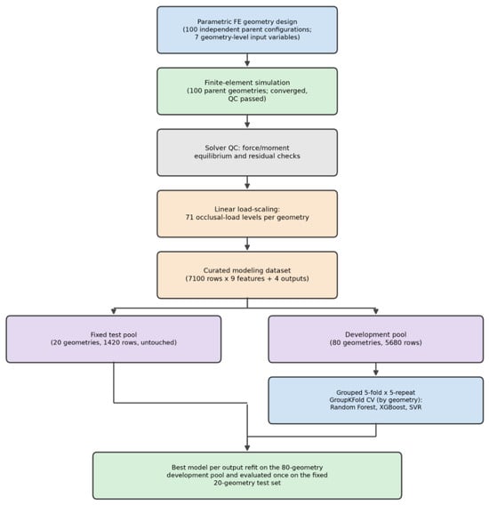
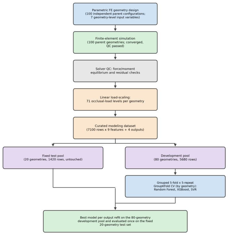
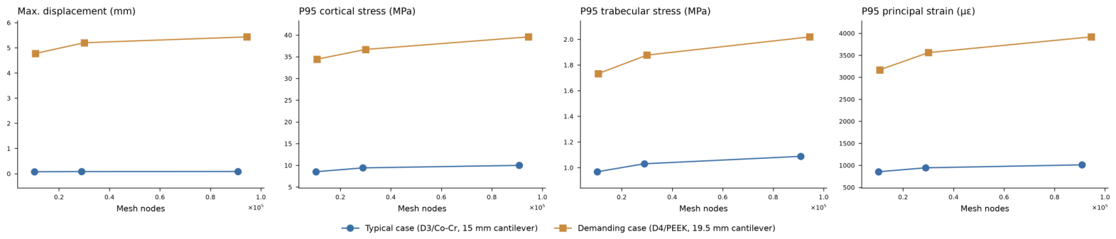
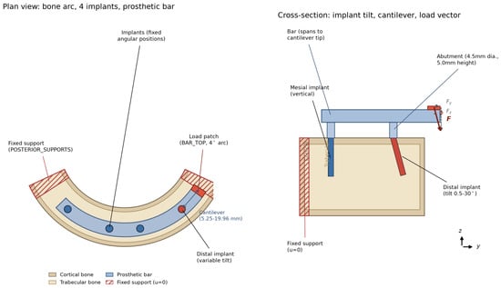
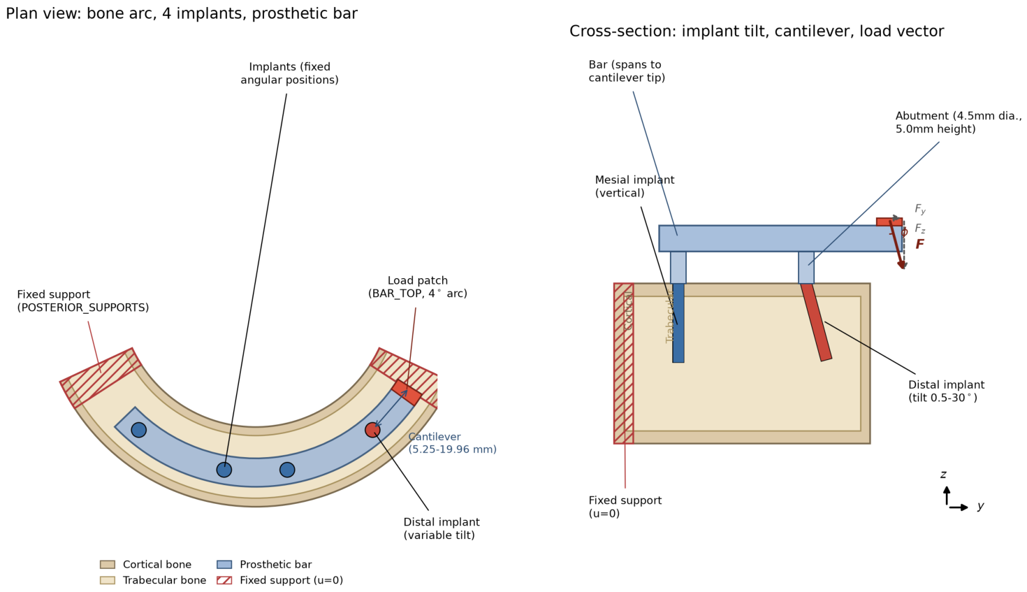
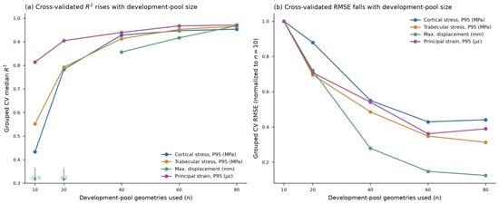
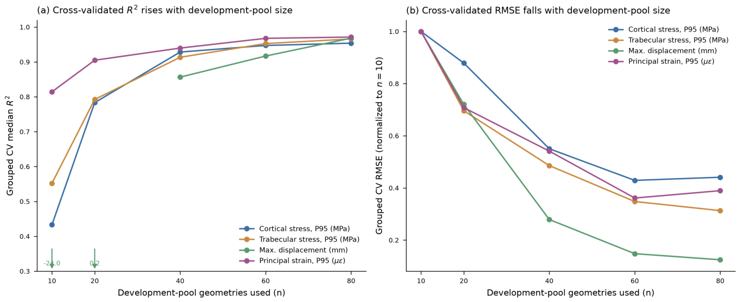
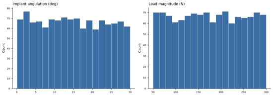
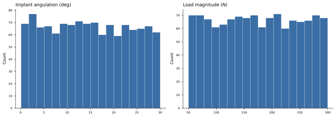
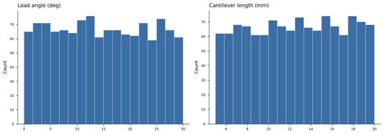
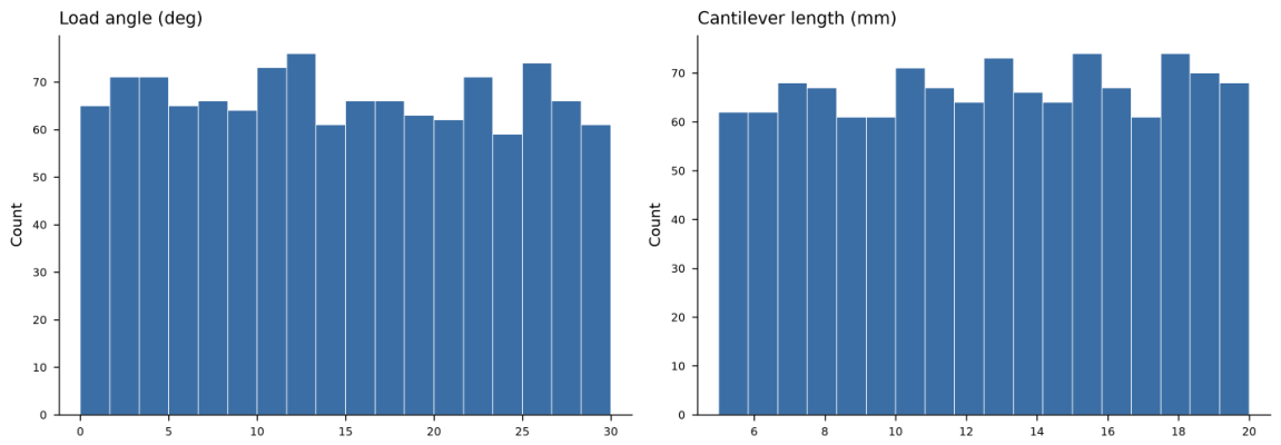
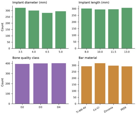
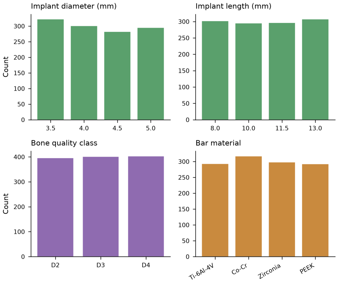
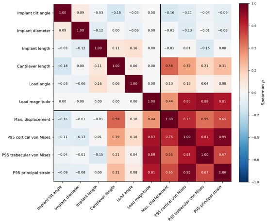
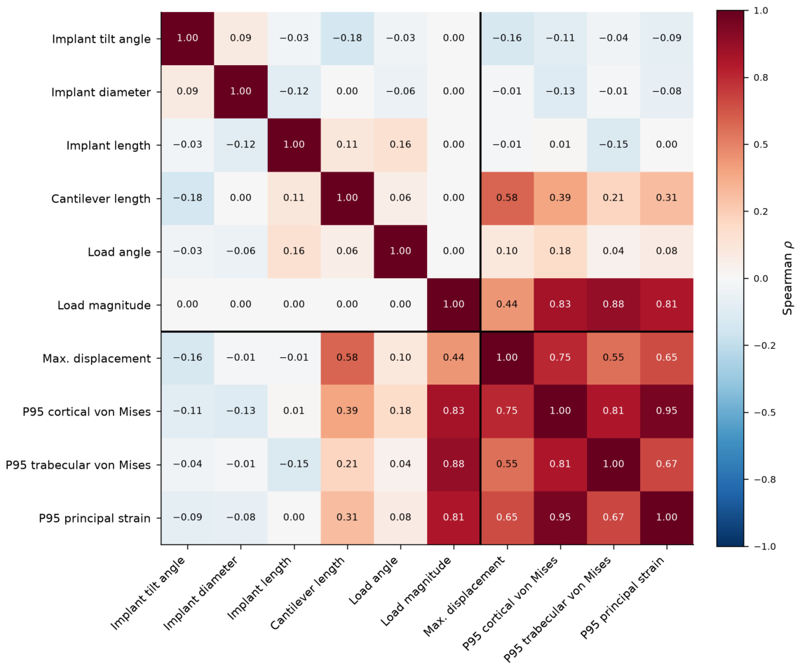
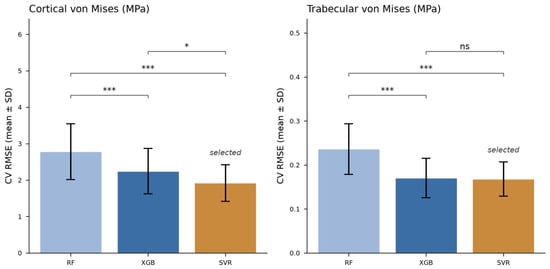
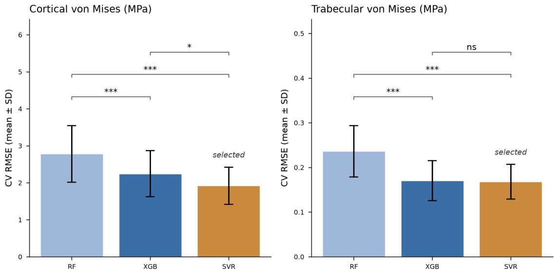
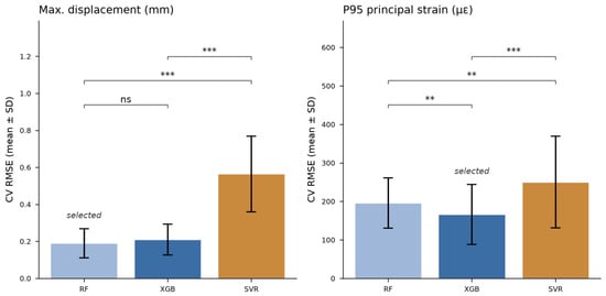
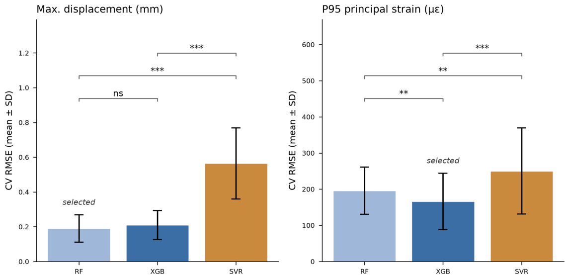
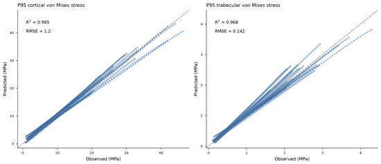
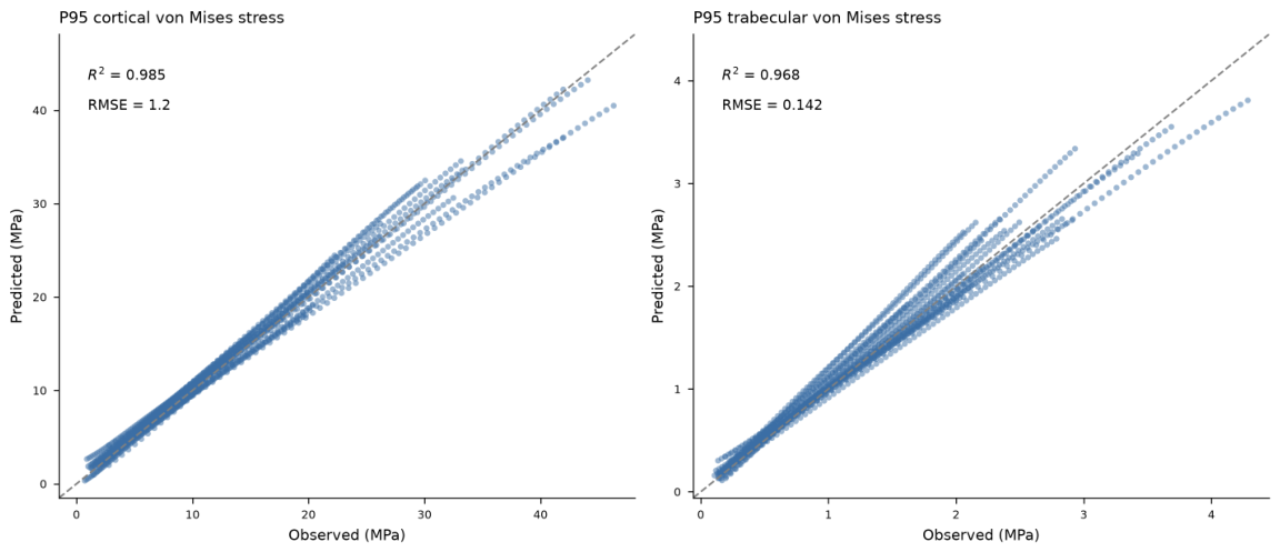
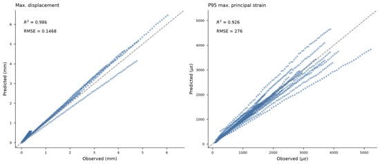
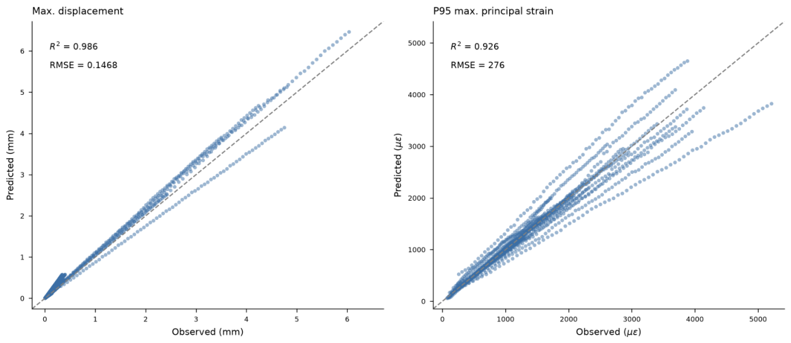
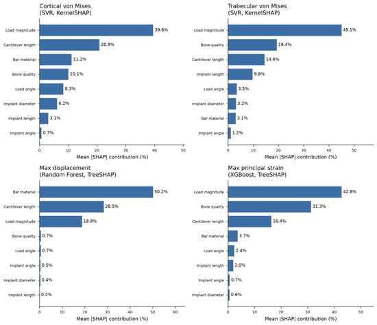
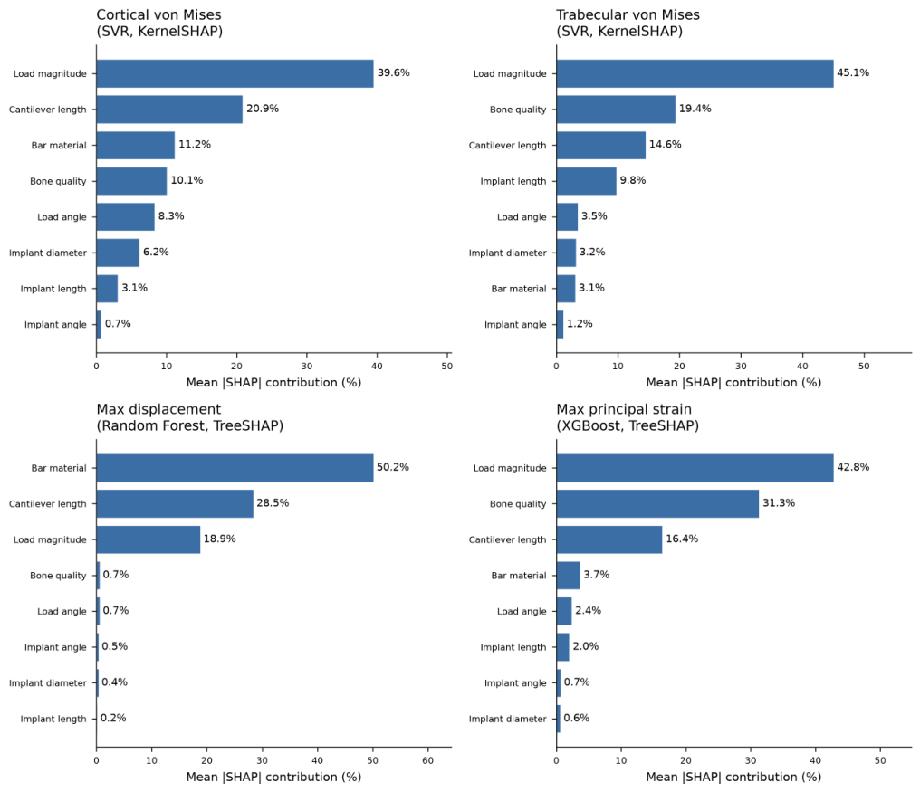
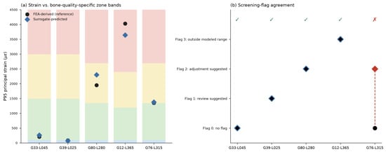
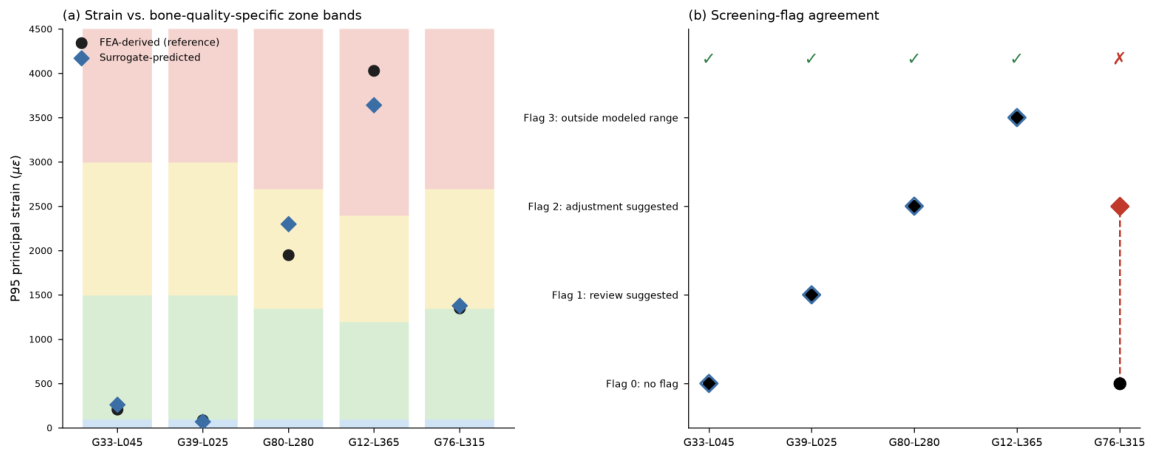
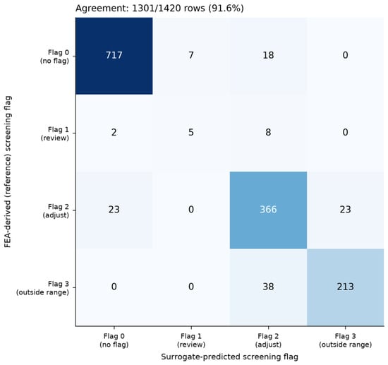
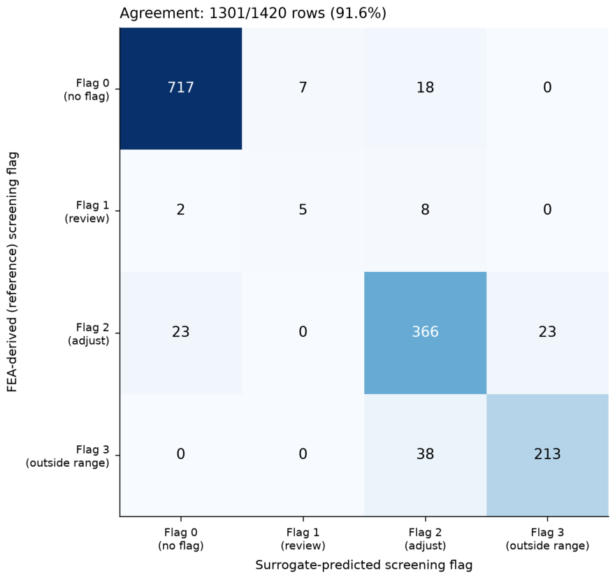

Disclaimer/Publisher’s Note: The statements, opinions and data contained in all publications are solely those of the individual author(s) and contributor(s) and not of MDPI and/or the editor(s). MDPI and/or the editor(s) disclaim responsibility for any injury to people or property resulting from any ideas, methods, instructions or products referred to in the content. |
© 2026 by the authors. Licensee MDPI, Basel, Switzerland. This article is an open access article distributed under the terms and conditions of the Creative Commons Attribution (CC BY) license.