


Abstract
Detecting small, distant ground vehicles in real time on edge hardware requires models that jointly balance accuracy, computational efficiency, and robustness to degraded imagery; therefore, deployment suitability cannot be inferred from accuracy on general-purpose benchmarks alone. This study compares five detection architectures spanning two-stage and one-stage families under a standardized experimental protocol, using a purpose-built dataset of 5501 annotated frames covering three classes of ground vehicles. Each configuration was trained with three random seeds using a leakage-controlled data split, evaluated under a unified detection protocol, benchmarked directly on an NVIDIA Jetson Orin Nano Super, and tested using a reproducible, probability-based corruption protocol. To the best of our knowledge, no previous study has evaluated both detector families on a common ground-vehicle dataset dominated by small and distant instances, within a single framework combining multi-seed variance analysis, on-device performance measurement, controlled corruption testing, and training-protocol sensitivity analysis. Under each architecture’s canonical training regime, YOLO11n (mAP@0.5 = 0.811 ± 0.004) and YOLOv8n (0.807 ± 0.010) achieved comparable detection accuracy, outperforming the strongest two-stage configuration (0.775 ± 0.003) with substantially fewer parameters; disabling YOLO’s canonical online augmentation reversed this ranking. On the target edge platform, the one-stage models reached up to 61 FPS under TensorRT deployment, whereas Faster R-CNN configurations achieved, at most, 2.6 FPS. Under image corruption, Faster R-CNN retained 82.6% of its clean accuracy without corruption-specific training, exceeding YOLO’s 74.6–74.8% retention even after corruption-aware retraining from a 58.7–60.0% baseline. These results show that newer detector generations do not necessarily yield measurable gains in accuracy and that rankings can depend on training protocol choices; architecture selection should instead jointly weigh accuracy, latency, computational cost, and robustness. Under the evaluated conditions, compact one-stage detectors remain the most favorable deployment trade-off, while the standardized framework offers a reproducible basis for evaluating future architectures and edge platforms.
1. Introduction
Object detection has become one of the most widely deployed capabilities in modern computer vision. It enables automated systems to locate and classify objects in images and video streams and now underpins applications ranging from autonomous navigation and industrial inspection to medical imaging and security surveillance [1]. As these systems move from offline analysis toward live, on-device operation, detection is increasingly expected to run in real time rather than as a post-processing step.
This shift makes inference speed a first-order requirement rather than a secondary concern. In a streaming setting, the value of a detection depends not only on whether it is correct but on whether it arrives in time to act on. A system that processes each frame too slowly cannot support decisions that must be made as events unfold, regardless of how accurate its predictions are in isolation. Real-time object detection, therefore, couples two demands that are often in tension: high detection accuracy and low inference latency.
Defense and security operations are among the domains where this coupling is most consequential. Automated detection supports field monitoring, reconnaissance, and target identification, where the reliable recognition of potentially hostile objects directly informs operational decisions and reduces risk to personnel and civilians [2,3]. In these settings, the time available to act is short, and the cost of a missed or delayed detection is high, which makes real-time performance a defining requirement rather than a desirable feature.
Reliable detection in this domain is therefore essential for situational awareness and effective decision-making. An automated system intended for this role must quickly and accurately identify and localize armored vehicles, such as tanks, infantry fighting vehicles (BMPs), and armored transporters (BTRs), to support action as events unfold. Meeting this requirement in realistic operational settings involves several constraints that interact rather than apply in isolation:
- Real-time constraints. Detection must keep pace with a live video stream on the available hardware. A prediction that arrives too late to inform a decision provides no operational value, regardless of its accuracy, which places a firm lower bound on acceptable inference speed.
- Challenging and uncontrolled conditions. Operational imagery departs sharply from curated benchmarks. Targets vary in scale and orientation, are frequently small or distant, and are often partially occluded or degraded by smoke, dust, and poor visibility. A deployable model must remain reliable under these conditions, not only on clean data.
- Accuracy and reliability. Speed cannot be obtained at the expense of detection quality. Missed detections and false alarms both carry operational costs, so a usable model must maintain high precision and recall rather than trade one for the other to improve throughput.
- Edge-deployment limits. Operational systems typically run on embedded hardware rather than on data-center GPUs. Constraints on compute, memory, and power restrict which architectures are viable and determine the accuracy a model can deliver within a fixed on-device latency budget.
These constraints rarely point to the same model. Architectures differ in how they allocate capacity between accuracy and inference speed: two-stage detectors generally favor accuracy, while one-stage detectors favor speed, and edge hardware further narrows the set of usable options. Consequently, the most accurate model in absolute terms is often not the most suitable once real-time and on-device limits are imposed.
The problem addressed in this paper, therefore, has two coupled parts. The first is informed model selection, determining which detection architecture offers the most favorable balance of accuracy, robustness, and inference speed for real-time armored vehicle recognition on edge hardware. The second is establishing the conditions under which such a selection can be made reliably. This requires a dataset representative of operational imagery, built specifically for this task; training recipes applied consistently across architectures, so that measured differences reflect the models themselves rather than differences in how they were trained; and inference benchmarking conducted on the target edge device rather than estimated on desktop hardware. Addressing both parts is what separates a defensible answer from an arbitrary one: a ranking produced without controlled training conditions, on data unrepresentative of the domain, or with speed estimated rather than measured on the target device would offer no reliable guidance for deployment.
This paper accordingly develops and evaluates object detection models for real-time armored vehicle recognition, with a focus on deployment under realistic operational and hardware constraints. The study targets three representative armored vehicle classes: tanks, infantry fighting vehicles (BMPs), and armored transporters (BTRs) and assesses both detection accuracy and inference performance, including behavior on edge hardware and under degraded visual conditions.
The main contributions of this study are as follows:
- A purpose-built dataset of 5501 annotated frames of armored vehicles, extracted from real operational footage and covering three target classes across varied terrain, viewpoint, scale, and visibility conditions, addressing the scarcity of openly available datasets for this domain [4,5]. Augmentation is applied only after the train/validation/test split is fixed, so that no augmented variant of a training image can appear in either evaluation subset.
- A standardized training and evaluation protocol under which five detection architectures spanning the two-stage and one-stage families are compared, with three seeds per configuration and all results reported as mean ± standard deviation, so that measured differences are attributable to the architectures rather than to training conditions or single-run variance.
- On-device deployment measurements on the NVIDIA Jetson Orin Nano Super, reporting throughput, latency, and energy per frame at explicitly stated inference precision and runtime, rather than estimating edge performance from desktop hardware.
- A robustness evaluation under a reproducible, probability-based corruption protocol, using a three-condition design that isolates the effect of corruption-aware training on the selected architectures.
The scientific novelty of this work lies in establishing a controlled cross-family experimental framework in which detection accuracy, edge-device efficiency, and robustness to corruption are evaluated jointly under identical data, training, and evaluation conditions. Previous studies have examined detector accuracy, edge deployment, or robustness separately, and comparable robustness studies have largely focused on civilian traffic imagery. At the same time, edge-device benchmarks have often been limited to individual architecture families. As a result, findings reported across such studies cannot be directly combined into a reliable deployment decision.
By evaluating these dimensions simultaneously, the present study provides new empirical evidence about the trade-offs between detector architecture, predictive performance, computational efficiency, energy cost, and robustness in the specific context of armored vehicle detection on resource-constrained edge hardware. In particular, the results show that a newer detector generation does not necessarily produce a measurable gain in detection accuracy under the examined task and data regime, while substantial differences remain in deployment efficiency and robustness. This finding indicates that model selection for operational edge deployment should not be based solely on architecture generation or clean-image accuracy, but on a joint assessment of accuracy, latency, energy consumption, and robustness.
Accordingly, the contribution of the proposed framework extends beyond the ranking of the five models evaluated in this study. It provides a reproducible experimental basis for assessing future detector architectures and hardware platforms under a common set of deployment-relevant criteria, thereby supporting more evidence-based model selection for real-time vision systems operating under constrained and potentially degraded conditions.
This paper is organized as follows: Section 2 reviews the most relevant literature on detection methods for this domain. Section 3 presents the materials and methods, comprising a comparative overview of two-stage and one-stage detection algorithms (Section 3.1), the creation and analysis of the custom dataset (Section 3.2), and the detection architectures with their standardized training procedures (Section 3.3). Section 4 presents the experimental setup and results, covering detection performance on the proposed dataset (Section 4.2), error analysis (Section 4.3), deployment performance on edge hardware (Section 4.4), robustness under degraded visual conditions (Section 4.5), and ablation studies isolating individual design choices (Section 4.6). Section 5 discusses the findings in relation to existing research. Finally, Section 6 concludes the paper and outlines directions for future work.
2. Related Work
Deep learning has become the dominant approach for detecting armored vehicles and other heavy equipment, in which reliable recognition directly informs reconnaissance and command decisions. Detection rarely stands alone: its output feeds downstream decision-support and threat-assessment systems, where accuracy and timeliness shape the quality of the resulting decisions [2]. Convolutional detectors, and the YOLO family in particular, now achieve high accuracy on this task without specialized sensing hardware. Deployment in the field, however, imposes requirements that extend beyond detection accuracy alone: models must run within tight latency budgets, on embedded platforms with limited compute and power, and remain reliable under visually degraded conditions. The following review groups prior work by these requirements and identifies, for each, the gap this study addresses.
The first body of work directly targets the detection of armored ground vehicles. Several studies adapt YOLO-family detectors to these targets and report high accuracy on custom datasets, often introducing lightweight backbones or attention modules to reduce computational cost for constrained platforms [3,4,6]. A recurring theme across this work is the scarcity of suitable data: because imagery in this domain is limited by confidentiality and has few public benchmarks, authors are repeatedly forced to construct their own datasets before training [4,5]. Gupta et al., for example, note the absence of an openly available dataset with diverse vehicle classes and assemble one specifically to train and compare lightweight detectors on edge devices [5]. This dependence on bespoke datasets is a shared constraint rather than an incidental detail, and it motivates the construction of a purpose-built dataset in the present study. The same body of work tends to optimize for accuracy on clean imagery, with deployment behavior and robustness reported only secondarily.
A second line of research compares two-stage and one-stage detectors to characterize the speed–accuracy trade-off. Huang et al. survey this trade-off across detector families and note that direct, like-for-like comparison is difficult because reported results differ in their backbones, input resolutions, and hardware [7]. On real-world data, the trade-off is not always settled in favor of speed: Carranza-García et al. evaluate one-stage and two-stage detectors on a large autonomous driving benchmark and find that the two-stage Faster R-CNN remains more accurate and more reliable for underrepresented classes, even as one-stage models retain a clear speed advantage [8]. These comparisons are typically conducted on general-purpose civilian benchmarks rather than on the target classes examined here and rarely under the deployment constraints that determine which detector is actually usable in the field.
A third group of studies evaluates detectors on embedded hardware, where inference speed and energy use become first-order metrics. Recent work benchmarks YOLO-family models across Jetson-class devices and quantization settings, reporting frame rates and energy consumption under FP32, FP16, and INT8 precision [9]. Rey et al., evaluating lightweight YOLOv8 variants on the NVIDIA Jetson Orin Nano and Orin NX, show that real-time throughput on these platforms depends strongly on the device and the precision used, with the smallest model reaching real-time rates only under reduced precision [9]. Such studies establish that edge viability cannot be inferred from desktop results, but they generally benchmark a single architecture family and report metrics without a sufficiently precise specification for fair comparisons across architectures.
A fourth line of work examines robustness under degraded visual conditions. Gholinavaz et al. compare YOLO variants and Faster R-CNN on adverse-weather imagery augmented with noise and blur, finding that the most accurate model on clean data is not the most resilient under degradation, and conclude that environment-aware evaluation is necessary for real-world reliability [10]. Related work improves robustness to specific effects such as fog or motion blur through architectural or preprocessing changes [3]. This research establishes that degraded conditions materially change model rankings, but it is largely confined to civilian domains and to ad hoc degradations rather than to a systematic, reproducible corruption protocol applied to a held-out test set.
Within the one-stage family itself, architectural turnover has been rapid, and comparative reviews now document a clear generational trajectory. Sapkota and Karkee trace the Ultralytics lineage from YOLOv5, which established a modular PyTorch implementation with a PANet neck, through YOLOv8, which introduced an anchor-free decoupled head and the C2f aggregation module, to YOLO11, which replaced C2f with more compact C3k2 blocks and added a spatial-attention module [11]. Their COCO benchmark quantifies the effect: at an equivalent parameter budget of 2.6 M, YOLOv5u-n reaches 34.3% mAP@0.5:0.95, while YOLO11n reaches 39.5%, with YOLOv8n intermediate at 37.3% using 3.2 M parameters [11]. The lineage has continued past YOLO11 with YOLO26, which removes distribution focal loss and non-maximum suppression to reduce export friction and quantization sensitivity on embedded hardware [12]. In parallel, community-maintained releases outside the Ultralytics line have pursued separate directions, including programmable gradient information in YOLOv9 [13], NMS-free dual-assignment training in YOLOv10 [14], and attention-centric designs in YOLOv12 [15]. The present study evaluates YOLOv8 and YOLO11 as representatives of this family. Both are maintained within a single framework, which allows them to be trained under one canonical regime so that the difference between them reflects architecture rather than differing reference implementations; earlier releases such as YOLOv5 are superseded at equivalent model size by the figures above, while the community-maintained variants would each introduce a distinct reference recipe and thereby weaken the controlled comparison this study is designed to support.
A separate line of work replaces convolutional detection components with transformer mechanisms. RT-DETR removes non-maximum suppression through an end-to-end design built on a hybrid encoder that decouples intra-scale interactions from cross-scale fusion, achieving accuracy exceeding that of comparable YOLO detectors on the COCO dataset [16]. Its behavior on embedded hardware, however, differs from its behavior on server-class GPUs in ways that matter for the deployment regime examined here. In a recent comparison of YOLOv8 and RT-DETR across Jetson-class and single-board platforms, Suchý and Turčaník report that the relative ranking of the two architectures depends on runtime realization rather than on nominal computational cost and that the transformer detector incurs higher latency and energy per unit of nominal work across the evaluated runtimes even where its total FLOP count is lower [17]. They further report that RT-DETR could not be deployed at all on the NPU accelerators tested, since the associated compilers are optimized for the static graph structures typical of convolutional networks and do not support the required attention operations, and that the transformer model loses a larger fraction of its accuracy during export to a compiled runtime than its convolutional counterpart [17]. Transformer-based detectors are therefore acknowledged here as a relevant and rapidly developing branch, but they are not evaluated in this study, whose scope is the established two-stage and one-stage convolutional families compared under a common training regime and a common export path.
Across these lines, prior work tends to optimize accuracy on clean data within a single architecture family, validate on desktop hardware, and treat robustness and deployment as secondary concerns, with comparisons drawn from civilian benchmarks under inconsistent training and evaluation conditions. This study addresses that combination directly. It compares two-stage and one-stage detectors across both families under standardized, family-appropriate training and a single unified evaluation protocol on a purpose-built ground-vehicle dataset; it benchmarks the trained models on the target edge device, the NVIDIA Jetson Orin Nano Super (NVIDIA Corporation, Santa Clara, CA, USA), with inference precision stated explicitly; and it evaluates robustness on a reproducible corruption test set derived from the original test split. Together, these elements provide not a single ranking but a fair and reproducible basis for selecting a detection architecture for this domain. The evaluation is deliberately bounded to these two families; extending the same protocol to transformer-based detectors and to more recent one-stage releases is a direct continuation of the apparatus rather than a revision of it.
3. Materials and Methods
3.1. Two-Stage vs. One-Stage Detectors
Modern object detectors are commonly divided into two families that differ in how they convert an image into a set of detections. The distinction is mechanical, and it is the source of the speed-accuracy trade-off that governs model selection for real-time use.
Two-stage detectors separate detection into proposal and classification. A first stage scans the image and proposes regions that are likely to contain objects; a second stage then classifies each proposed region and refines its bounding box. Faster R-CNN [18,19,20,21] is a representative example, generating proposals through a region proposal network (RPN) [22] that shares features with the classification stage, thereby eliminating the cost of external proposal methods. Concentrating computation on a limited set of promising regions yields high localization accuracy, particularly for small or densely arranged objects, but processing the image in two passes increases inference cost and constrains real-time deployment, especially on edge hardware.
One-stage detectors remove the proposal stage and predict object classes and bounding boxes directly from feature maps in a single pass. SSD [23] performs detection across multiple feature maps so that objects of different sizes are handled at different scales, while YOLO [24,25,26] divides the image into a grid and predicts detections for each cell simultaneously. Predicting everything in a single pass makes these detectors substantially faster and well-suited to streaming input, though the absence of a dedicated proposal stage has historically reduced accuracy for small and partially occluded objects. Successive YOLO generations have narrowed this gap through improved feature aggregation, anchor-free prediction, and refined loss functions.
Although the two families are defined by distinct mechanisms, the accuracy gap between them is not fixed. RetinaNet [27] illustrates this: it is a one-stage detector, but it approaches two-stage accuracy by introducing Focal Loss to counter the foreground–background class imbalance that single-pass detectors face and by combining it with a feature pyramid network (FPN) [28] for multi-scale detection. It is not evaluated in this study, but it shows that the accuracy gap can be narrowed through design rather than solely by adding a proposal stage, a principle since extended by transformer-based detectors discussed in Section 2, which is precisely why an empirical comparison in a specific domain and on a target device is necessary rather than assuming the trade-off based on architecture type alone.
In summary, the choice between detector families is a choice about where to spend a fixed computational budget: two-stage designs invest it in accuracy through region refinement, while one-stage designs invest it in throughput through single-pass prediction, with hybrid designs such as RetinaNet occupying the space between. This study samples the trade-off rather than a single point on it. The two-stage family is represented by Faster R-CNN with two backbones of differing capacity, a lightweight MobileNetV3 variant and a higher-capacity ResNet-50 FPN, allowing the accuracy-cost trade-off to be observed within a single architecture. The one-stage family is represented by SSD with a MobileNetV3 backbone and by two YOLO generations, YOLOv8 and YOLO11, selected for the reasons set out in Section 2 as representatives of a single framework’s canonical training regime. Evaluating these models under consistent conditions, on a common dataset, and on the target edge device allows the trade-off to be resolved for this domain rather than assumed.
3.2. Dataset
This section describes the construction and characterization of the dataset used throughout the study. It covers the frame extraction and annotation procedure, the resulting class and scale distribution, the train/validation/test partitioning and the safeguards applied to it, and the automated integrity checks performed before training.
A central requirement of this study is a dataset that reflects the conditions under which armored vehicle detection must operate. No public dataset covers the target classes with the diversity and realism required, a limitation noted repeatedly in earlier studies [4,5]. A purpose-built dataset was therefore constructed from real operational footage, following the pipeline shown in Figure 1.
Figure 1.
Dataset construction pipeline represented as an event-driven process chain (EPC): pink hexagons denote events (states), green rectangles denote functions (activities), and blue-bordered objects denote the software system supporting each function, connected to it by a dashed line.
The pipeline proceeds through video collection, import, frame extraction, and image preprocessing before annotation, splitting, and augmentation. Figure 1 represents this pipeline as an event-driven process chain (EPC), a notation in which states (events, shown as hexagons) and activities (functions, shown as rectangles) strictly alternate, so that every processing step carries an explicit precondition and outcome rather than an implied one. Each function is further linked, where applicable, to the software system used to execute it: video import and frame extraction were carried out in Adobe Premiere Pro (version 25.0; Adobe Inc., San Jose, CA, USA), image preprocessing in Python (version 3.13.15) with OpenCV (version 5.0.0), annotation in LabelImg (version 1.8.6), dataset splitting in Roboflow (Roboflow, Inc., Des Moines, IA, USA), offline augmentation with the Albumentations framework (version 2.0.8), and training integration through Ultralytics and PyTorch on Google Colab (Google LLC, Mountain View, CA, USA).
Frame extraction retains only a small number of visually distinct frames per source video, typically four to five per 1- to 2-min clip, to limit redundancy at the source. Augmentation is applied only to the training split, and only after the split has been fixed, so that no augmented variant of a training image can appear in either evaluation subset.
The dataset targets three classes of armored vehicles: tanks, infantry fighting vehicles (BMPs), and armored transporters (BTRs). Source frames were extracted from operational videos captured across varied terrain, seasons, viewpoints, and imaging conditions, including ground-level, elevated, and aerial perspectives. This variety is deliberate: it exposes the models to the scale, orientation, occlusion, and visibility changes characteristic of operational imagery rather than to a narrow, curated distribution. Figure 2 shows representative annotated samples across the three classes and the range of conditions present.
Figure 2.
Representative annotated dataset samples across the three target classes (BMP, BTR, and tank), illustrating the range of terrain, viewpoint, scale, and visibility conditions.
After extraction and cleaning, the dataset comprises 5501 distinct annotated frames. During preprocessing, images were auto-oriented to normalize EXIF rotation, and resolution was standardized per architecture to match each model’s expected input: 1280 × 720 for Faster R-CNN, 640 × 640 for YOLO, and 320 × 320 for SSD, so that every model received data in its native format without penalizing any architecture through mismatched scaling. Annotation was performed with bounding boxes for the three classes.
The dataset was divided into training, validation, and test subsets of 4185, 1017, and 299 images, respectively, with an approximate 76/19/5 split, preserving class balance across all three. Frame extraction was itself designed to limit redundancy at the source: from each source video, only a small number of visually distinct frames were retained, with adjacent or near-identical moments deliberately excluded. Augmentation was applied only to the training split, and only after the split had been fixed. This ordering is a deliberate control: because every augmented image is generated from a frame already assigned to training, no augmented variant of a training image can appear in the validation or test subsets. The dataset does not enforce a source-video-level split, so frames from the same video, and occasionally the same vehicle instance viewed from a substantially different angle, may appear across different subsets; the deliberate diversity of extracted frames limits how similar such cases can be, but this is a curation practice rather than a formal split-time guarantee. The augmentation set comprised brightness variation, mild noise (1%), horizontal flipping, and small rotations (−5° to +5°), expanding the training split fourfold to 16,740 images. The complete dataset contains 18,056 images and 31,545 annotations across all subsets.
To assess residual similarity across the split, an embedding-based nearest-neighbor search was performed for each test image against the training set. Each image was encoded with a ResNet-50 backbone pretrained on ImageNet, using global-average-pooled features, and similarity was measured by cosine distance between L2-normalized embeddings. For each test image, the single most similar training image was identified, and the resulting similarity scores were aggregated across the full test set. Similarity was moderate on average (mean 0.774, median 0.772, standard deviation 0.100), consistent with visually related but distinct content across most of the test set. Table 1 reports the fraction of test images whose nearest training match exceeds several similarity thresholds. At a strict threshold of 0.98, only a single test image (0.3%) returns a near-duplicate-range match; at 0.95, five images (1.7%) do so. This check does not by itself establish source-video independence, since video identity could not be recovered at the extraction stage, but it provides a direct, quantified measure of visual redundancy between the two subsets, alongside the curation practice described above.
Table 1.
Fraction of test images with a nearest-neighbor training-set match above each similarity threshold.
To support a separate robustness evaluation, two additional data artifacts were derived from the same source frame pool. A degraded training split applies stronger perturbations: 1% noise, Gaussian blur (0.3–0.8 px), and motion blur (10 px length), in addition to the original augmentations, to train a corruption-aware model. A corruption test set applies probability-triggered degradations to the held-out imagery, providing an evaluation target that no model has seen during training. These splits were repartitioned from the source pool with enlarged validation and test subsets, as detailed in Section 4.5; they are used only in the YOLO robustness analysis and do not affect the primary cross-architecture comparison.
The dataset’s composition was analyzed to characterize the detection problem it poses. Figure 3 shows the distribution of object sizes by class, expressed as the fraction of image area each object occupies. A large proportion of objects, most pronounced for BMPs and tanks, falls within the smallest size band (0–1% of the image area), indicating a prevalence of small, distant targets. A secondary concentration of larger objects (9–100%) reflects close-range views, giving the dataset a wide scale range that any detector must handle.
Figure 3.
Distribution of object size by class, as a percentage of image area across five size bands.
The spatial and geometric distribution of annotations further characterizes the task (Figure 4). Figure 4a shows bounding-box center density: objects concentrate toward the image center but occur across the full frame. The central bias is expected for operator-captured footage, where the camera tends to be aimed at the target; importantly, however, coverage of the periphery remains substantial, so models cannot exploit position as a shortcut and must detect objects wherever they appear. Figure 4b shows the joint distribution of normalized box width and height. Annotations concentrate on small dimensions, consistent with the size analysis of Figure 3, while a spread toward larger boxes preserves close-range instances. The distribution also reflects the geometry of the target classes: box shapes cluster around moderate aspect ratios rather than extreme elongations, which keeps them within the operating range of the anchor-based detectors’ default box configurations and requires no per-model anchor tuning, consistent with the no-modification principle applied in Section 3.3.1. Taken together, the two panels define the detection problem the dataset poses: targets may appear anywhere in the frame, at scales dominated by small instances, a combination that stresses precisely the multi-scale and small-object capabilities on which the compared architectures differ most.
Figure 4.
Spatial and geometric distribution of annotations in normalized image coordinates (log-scaled annotation count per cell): (a) bounding-box center density; (b) object size density over bounding-box width and height.
The dataset was validated for annotation integrity before training. Automated checks screened for missing or corrupt image files, unknown category IDs, orphan annotations, images without valid annotations, degenerate and out-of-bounds boxes, extreme aspect ratios, tiny boxes, and duplicate annotations. Most checks returned no violations. Figure 5 reports the three categories that did occur, all at low rates. Tiny boxes (<0.3% area) are the most frequent, at 14–18% across splits, which is consistent with the small-object prevalence seen in Figure 3 rather than an annotation fault; out-of-bounds boxes and extreme aspect ratios each remain below 4%. This profile indicates the dataset is clean enough for reliable training while retaining the genuinely difficult small-object cases the task requires.
Figure 5.
Dataset validation: annotation quality profile, showing the percentage of boxes flagged by each non-zero integrity check across the train, validation, and test splits.
Taken together, these analyses characterize a dataset that is both realistic and deliberately challenging. It spans a wide range of object scales, viewpoints, and visibility conditions, with a pronounced concentration of small, distant targets that represents the hardest case for detection. Its integrity was verified prior to training, and its augmentation and split design ensure that measured performance reflects genuine generalization rather than leakage between subsets. This dataset forms the common basis on which all five detection architectures are trained and evaluated under identical conditions. The architectures and their standardized training procedure are described in Section 3.3.
3.3. Methods
This section describes the detection architectures evaluated in this study and the training procedure applied to them. Section 3.3.1 states the design principles that ensure measured differences reflect the architectures themselves; Section 3.3.2 and Section 3.3.3 describe the two-stage and one-stage architectures, respectively; Section 3.3.4 specifies the standardized training recipe applied across all five models.
3.3.1. Design Principles
The methods in this study serve a practical objective: identifying a detection architecture that can be deployed for real-time armored vehicle recognition on edge hardware, with accuracy, speed, and robustness adequate to operational use. Answering this requires more than training several models; it requires a comparison in which measured differences reflect the architectures themselves rather than differences in how they were trained, since only then can the outcome support a deployment decision. Three principles enforce this. First, all five models are initialized with COCO-pretrained weights and used without architectural modifications: no custom anchors, backbone changes, or per-model structural tuning are applied, since any such adjustment would turn the comparison into a per-model improvement study. Second, all models are trained and evaluated on the identical dataset described in Section 3.2: the same split, the same augmented training set, and the same held-out test subset. The YOLO models additionally apply the online augmentation used in their native training frameworks; this is deliberately retained, as it is part of the canonical regime under which these architectures are published and reproduced. Third, every model is trained with three random seeds (0, 1, and 2) under a fixed epoch budget, and all results are reported as mean ± standard deviation across seeds, so that single-run variance cannot masquerade as an architectural difference. Training regimes are standardized at two levels. The TorchVision detectors, both Faster R-CNN variants and SSDLite, share one common recipe that removes optimizer and schedule differences as a confound within that family. The YOLO models are trained under the canonical regime of the Ultralytics framework, which constitutes their published identity. Both regimes, and the settings in which they differ, are specified in Section 3.3.4. Data, pretraining, epoch budget, seeds, and evaluation protocol remain identical across all five models.
3.3.2. Two-Stage Detectors: Faster R-CNN
Faster R-CNN decomposes detection into proposal generation and region classification. A backbone network extracts a feature representation of the input image; a region proposal network (RPN) slides over these features and proposes candidate object regions; a detection head classifies each proposed region and refines its bounding box. Both stages are trained jointly by minimizing a multitask objective combining classification and localization terms [22]:
where is the predicted object probability for anchor ; is its ground-truth label; and are the predicted and target box regression parameters; is a log loss over object/background; is a smooth- loss active only for positive anchors (); and is a balancing weight. The same loss form applies in both the RPN and the detection head, so accuracy is refined twice—once when regions are proposed and again when they are classified, which is the mechanical source of the family’s localization strength and of its additional inference cost.
Two backbone configurations are evaluated, chosen to span the capacity range within a single architecture (Figure 6). The first employs ResNet-50 with Feature Pyramid Network V2, providing deep residual feature extraction with multi-scale fusion. The second replaces the backbone with MobileNetV3-Large FPN, a lightweight alternative designed for constrained hardware. Comparing the two isolates, the contribution of backbone capacity while the detection mechanism is held fixed.
Figure 6.
Faster R-CNN architecture with the ResNet-50 FPN backbone.
In both configurations, the detection mechanism, loss, and training procedure are identical; only the backbone varies. This pairing provides the study’s controlled view of the accuracy-cost trade-off inside the two-stage family, complementing the cross-family comparison with the one-stage detectors described next.
3.3.3. One-Stage Detectors: SSDLite and YOLO
One-stage detectors remove the proposal stage and predict classes and boxes directly from feature maps. SSD performs this prediction over a set of default boxes tiled across feature maps of several resolutions, so that objects of different scales are matched at different levels. Training minimizes a weighted sum of confidence and localization losses over matched default boxes [23]:
where is the number of matched default boxes, is a softmax loss over class confidences ; is a smooth- loss between predicted boxes and ground truth ; and is a balancing weight. The contrast between Equations (1) and (2) expresses the two-stage/one-stage distinction of Section 3.1 in concrete form: Faster R-CNN applies its objective twice over a filtered set of candidate regions. In contrast, SSD applies a single objective once over a dense grid of default boxes, trading a second refinement pass for single-pass speed.
This study uses SSDLite320 with a MobileNetV3-Large backbone (Figure 7), a mobile-optimized SSD variant operating on 320 × 320 input images. SSDLite replaces the standard convolutions in the detection heads with depthwise separable convolutions, substantially reducing computation at a modest cost in capacity, and the MobileNetV3-Large backbone extends this efficiency to feature extraction through inverted residual blocks and hard-swish activations. The configuration represents the most efficient end of the model set: the smallest input resolution, the lightest heads, and the lowest computational budget among the five models. Its inclusion establishes the lower bound of the accuracy-efficiency trade-off: how much detection quality the task permits when computational cost is minimized as far as the standard toolset allows.
Figure 7.
SSDLite320 architecture with the MobileNetV3-Large backbone. The upper panel details the MobileNetV3 inverted residual block with squeeze-and-excitation, where denotes element-wise multiplication applying the channel-wise attention weights to the feature map; the lower panel shows the detection pipeline, in which two backbone levels and four SSDLite extra layers feed the detection heads. Feature map dimensions correspond to a 320×320 input.
The final pair of models comes from the YOLO family, which divides the image into a grid and predicts detections for all cells in a single forward pass. Every model in the family shares a three-part structure: a backbone extracts features, a neck aggregates them across scales, and a detection head produces class and box predictions (Figure 8). This study evaluates two recent generations of this design, YOLOv8 and YOLO11, selected for the reasons set out in Section 2, which differ in how the three components are implemented rather than in the overall scheme.
Figure 8.
Generalized YOLO detection architecture common to the YOLOv8 and YOLO11 generations: backbone stages P1–P5, a bidirectional feature-fusion neck, and three anchor-free decoupled detection heads. The dashed connector indicates that the box-regression and classification structure shown is shared identically across all three detection scales, rather than being repeated separately for each. Version-specific feature-aggregation modules are summarized in the lower panel. Feature map dimensions correspond to a 640 × 640 input.
YOLOv8 introduced an anchor-free, decoupled head that separates the classification and box-regression branches, along with the C2f feature-aggregation module to improve gradient flow and a distribution focal loss for box regression [29]. YOLO11 retains this anchor-free design while revising the backbone and neck to achieve greater parameter efficiency, achieving comparable or higher accuracy with reduced model size [30]. Their loss functions combine classification, box regression (CIoU), and distribution focal terms as defined in the respective framework implementations [29,30]; these are retained unchanged, consistent with the no-modification principle in Section 3.3.1.
Both models are used at 640 × 640 input in their small-capacity variants, matching the study’s edge-deployment focus. Together with SSDLite, they complete the one-stage family in this study, covering its efficiency extreme and its current accuracy-oriented designs; the cross-family comparison against the two-stage pair is carried out in Section 4.
3.3.4. Standardized Training Recipe
The three TorchVision detectors, both Faster R-CNN variants and SSDLite, are trained under a single common recipe. Its purpose is to remove differences in optimizers and schedules as a confound within that family, so that their results differ only where the architectures do. Optimization uses stochastic gradient descent with Nesterov momentum, in which parameters are updated through a velocity term evaluated at a look-ahead position:
with momentum and learning rate . SGD with momentum is preferred over adaptive optimizers because it provides a common, well-understood regime across all TorchVision models and avoids per-model differences in effective step sizes that adaptive methods introduce. This is precisely the confound this recipe is designed to remove.
Learning rates are differentiated by parameter group. The COCO-pretrained backbone is updated at , while the detection heads, which must adapt from the 91 COCO classes to the three target classes, are updated at . The 10-fold ratio perturbs transferred features slowly while allowing the reinitialized heads to converge quickly.
The learning rate follows a linear warmup over the first 500 iterations, then a cosine annealing schedule over the remaining training:
where is the current iteration after warmup, is the total post-warmup iterations, and . Warmup prevents divergence, while the reinitialized heads produce large early gradients; cosine decay then smoothly reduces the step size, avoiding the abrupt drops of step schedules.
Model weights are additionally tracked by an exponential moving average (EMA), updated after every optimization step:
with decay . The EMA weights , rather than the raw training weights, are used for validation, checkpoint selection, and final test evaluation, as they average out step-to-step noise and yield a more stable final model. Checkpoint selection is performed on validation mAP, not on training loss, so that the selected model reflects generalization rather than overfitting.
Training runs for a fixed budget of 50 epochs with batch size 8, without early stopping, so that every model receives an identical optimization budget. Gradients are clipped to a maximum norm of 5.0, weight decay is set to , and computation uses bfloat16 mixed precision. Each model is trained with three seeds (0, 1, and 2) controlling initialization and data ordering. The complete configuration is summarized in Table 2.
Table 2.
Training configuration: common recipe for the TorchVision detectors (Faster R-CNN ResNet-50 FPN V2, Faster R-CNN MobileNetV3-Large FPN, and SSDLite320) and canonical settings for the YOLO models (YOLOv8n, YOLO11n).
The YOLO models are trained under the resolved defaults of their framework, which follow the same broad logic as the common recipe but differ in constants and shape. Optimization likewise uses SGD with momentum 0.9, selected automatically by the framework; the learning rate starts at 0.01 after a three-epoch linear warmup and decays linearly, rather than by cosine, to a fraction = 0.01 of its initial value. An exponential moving average of the weights is maintained with decay 0.9999 and used for checkpoint selection, mirroring the role of Equation (5). Training additionally applies the framework’s online augmentation, including mosaic composition, HSV color shifts, flipping, and scaling, on top of the offline-augmented training set of Section 3.2. Early stopping is disabled to ensure the epoch budget matches the common recipe exactly, and each run is executed in deterministic mode using the same three seeds. The contribution of this online augmentation to YOLO’s reported accuracy is tested directly in Section 4.6.3, which retrains both YOLO models with it disabled and reports the resulting change in accuracy relative to the Table 3 baseline.
Table 3.
Detection performance on the test split (mean ± standard deviation over three seeds). Precision, recall, and F1 are reported at the maximum-F1 confidence threshold for each run, selected per seed on the validation split.
As Table 2 shows, the two regimes differ in schedule shape, regularization constants, and the presence of online augmentation. These differences are retained deliberately: overriding the framework defaults would train the YOLO models under conditions for which they were never designed, and the resulting comparison would reflect that mismatch rather than the architectures themselves.
4. Results
This section presents the experimental results of the study. Section 4.1 describes the experimental setup and the evaluation protocol common to all reported results. Section 4.2 reports detection performance across the five architectures on the primary test split. Section 4.3 analyzes the errors underlying these aggregate results by class and by object size. Section 4.4 reports deployment performance on the target edge platform. Section 4.5 evaluates the robustness of both deployment-viable and deployment-excluded architectures under degraded visual conditions. Section 4.6 isolates the marginal contribution of three design choices through targeted ablations.
4.1. Experimental Setup and Evaluation Protocol
All models were trained on NVIDIA RTX PRO 6000 Blackwell Server Edition GPUs (NVIDIA Corporation, Santa Clara, CA, USA) in the Google Colab environment, using the frameworks specified in Section 3.3.4: TorchVision 0.26.0 with PyTorch 2.11.0 (CUDA 12.8) for both Faster R-CNN variants and SSDLite and Ultralytics 8.4.95 for YOLOv8n and YOLO11n, with all versions pinned across runs. Every configuration was trained with seeds 0, 1, and 2, yielding 15 training runs for the primary comparison. For each run, the checkpoint selected based on validation performance was retained, and all reported test results were produced using the exponential moving-average weights of that checkpoint.
Deployment measurements were conducted on the NVIDIA Jetson Orin Nano Super Developer Kit running JetPack 6.1, with a fixed 15 W power profile. For each model, the seed-1 checkpoint was benchmarked with a batch size of 1 using the native PyTorch runtime at FP32 and FP16 precisions. Since throughput does not depend on the trained weights themselves, a single representative seed was used uniformly across all five models. TensorRT compilation (version 10.3.0) was additionally pursued for the YOLO models only, whose checkpoints were exported to ONNX and compiled to TensorRT engines directly on the device; the two-stage detectors and SSDLite embed non-maximum suppression and dynamic shapes in their computation graphs in a form that the standard export path does not support and were therefore benchmarked under PyTorch alone. On-device inference used Ultralytics 8.4.102, a later release than the 8.3.0 used for training; this does not affect the trained weights and is reported for completeness. Reported values, therefore, reflect the optimized on-device inference path at a stated precision and runtime, rather than an unspecified or framework-level configuration.
Detection quality is evaluated with the standard COCO-style protocol. A predicted box is matched to a ground-truth box through their intersection over union:
A prediction counts as a true positive when the IoU exceeds a threshold and the predicted class is correct. Precision and recall are then defined as follows:
where , , and denote true positives, false positives, and false negatives, respectively. Average precision for a class summarizes the precision-recall curve obtained by sweeping the detector’s confidence threshold:
where is the precision at the recall level . It is computed with the 101-point interpolation of the COCO protocol, and the mean average precision aggregates over the classes:
Results are reported at the matching threshold (mAP@0.5) and averaged over thresholds from 0.5 to 0.95 in steps of 0.05 (mAP@0.5:0.95), the former reflecting detection capability and the latter localization quality. Where per-class behavior is analyzed, is reported separately for each class, and object-size effects are examined using the COCO partition into small, medium, and large instances. Average precision on small objects is interpreted with caution throughout: the small-object subset of the test split contains few instances, so each detection carries substantial weight in the score; consequently, this metric shows the largest seed-to-seed variance of all reported quantities.
All quantitative results are aggregated across the three seeds and reported as mean ± standard deviation. Aggregation is performed at the level of final test metrics, not across training curves, and no run was excluded, restarted, or reselected after its result was known. The evaluation under degraded visual conditions in Section 4.5 follows this same protocol, with the evaluation target replaced by the corruption test set described in Section 3.2.
4.2. Detection Performance on the Proposed Dataset
This section establishes the study’s primary comparison: how the five architectures perform when trained and evaluated under the unified conditions outlined in Section 3.2 and Section 3.3. Three questions structure the analysis: how the two detector families rank on this task, whether the accuracy differences justify the models’ large size differences, and whether the shared training budget treated all architectures fairly.
Table 3 reports the test set performance of all five models, aggregated over three seeds. All values are produced by the evaluation protocol of Section 4.1, using the checkpoint selected on validation performance for each run.
The comparison yields a clear ordering. The two YOLO generations are the strongest models and are indistinguishable within seed-level variance: YOLO11n reaches mAP@0.5 of 0.811 ± 0.004 and YOLOv8n 0.807 ± 0.010, a nominal difference well within seed-level variance. Both exceed the strongest two-stage configuration, Faster R-CNN ResNet-50 FPN V2, at 0.775 ± 0.003 by 3.3–3.7 points while using roughly 14 times fewer parameters. The equivalence of the two generations is informative rather than incidental: for this task and data regime, the architectural revisions between them do not translate into measurable gains in accuracy, so the choice between the two can be made on deployment grounds rather than on accuracy alone.
Within the two-stage family, backbone capacity behaves as expected: the MobileNetV3-Large FPN variant reaches 0.735 ± 0.005, trailing the ResNet-50 configuration by four points and indicating that the lightweight backbone trades accuracy for its reduced computational footprint. The trade is unfavorable, however: YOLOv8n exceeds this variant’s accuracy with roughly six times fewer parameters, so the lightweight two-stage configuration is dominated on both accuracy and size, indicating that reducing the backbone does not rescue the two-stage design for edge budgets. SSDLite320 falls far below all other models at 0.508 ± 0.006, a gap whose origin the error analysis in Section 4.3 attributes to missed detections rather than misclassification and predominantly among small objects.
Figure 9 visualizes these relationships as an accuracy-size trade-off. The YOLO models occupy the favorable corner of the plane, achieving the highest accuracy with the smallest parameter budgets. At the same time, the two-stage configurations require an order-of-magnitude more parameters to approach, and SSDLite’s efficiency comes at a substantial cost to accuracy.
Figure 9.
Detection accuracy versus model size for the five evaluated models, with parameter count on a logarithmic axis. Markers show test mAP@0.5 (mean over three seeds); vertical bars indicate ± one standard deviation.
The comparisons in Table 3 and Figure 9 rest on final test metrics, which are meaningful only if the shared training budget allowed every architecture to reach its full performance. Figure 10 verifies this by showing the validation trajectory of each model over the fixed 50-epoch budget, plotting the seed with the median final validation performance for each model, and revealing a graded convergence ordering rather than a single profile. The two-stage models reach their best validation performance earliest, within the first two-fifths of training (best epochs 10–12 for the ResNet-50 configuration and 16–19 for MobileNetV3), after which their curves decline gently as the heads begin to overfit past the EMA optimum. SSDLite peaks near the training midpoint. The YOLO models improve for the longest, overtaking both two-stage curves around the midpoint of training and reaching their best validation performance between epochs 30 and 40, consistent with their online augmentation continually varying the training distribution; their curves ease downward only over the final epochs, after the framework turns off mosaic augmentation for the closing 10 epochs of training. All five models therefore attain their optimum well within the shared budget, and checkpoint selection on validation performance (Section 3.3.4) ensures that each model is evaluated at its own optimum rather than at the final epoch. This is the precondition for attributing the differences in Table 3 to the architectures themselves.
Figure 10.
Validation mAP@0.5 over the 50-epoch training budget for all five models. Each curve shows one complete training run, using the seed with the median final validation mAP across the three trained models per family, so that no model is represented by its best or worst run.
Together, these results answer the three questions posed at the start of this section. The one-stage YOLO models rank highest on this task, and their advantage stems from their smaller model sizes compared to the others. At the same time, the two-stage configurations require an order-of-magnitude more parameters to approach, and SSDLite trades too much accuracy for its efficiency. The convergence analysis indicates that these differences are not artifacts of the training budget. Every model reached its optimum within the shared 50 epochs and was evaluated at its own best checkpoint. What the accuracy ranking alone cannot settle is the deployment decision, since the ResNet-50 configuration’s result, only a few points behind the YOLO models, would justify its selection if throughput were not a constraint. Section 4.4 resolves this on the target edge device. The aggregate metrics also conceal systematic per-class and size-dependent structure shared across architectures, which Section 4.3 examines first.
4.3. Error Analysis
The aggregate metrics in Section 4.2 average over classes, object sizes, and error types, thereby concealing structure that is consistent across architectures and directly relevant to operational use. Three questions guide the analysis in this section: whether the three vehicle classes are equally detectable, how strongly performance depends on object scale, and what actually happens to the objects a model fails to detect: confusion with another class or no detection at all.
The three classes are not equally detectable, and the pattern is remarkably consistent: Tank is the weakest class across all models with functioning small-object detection (Figure 11). The gap is widest for the YOLO models, which reach 0.84–0.88 on BMP and BTR but only 0.72 on Tank, and narrower but present for both Faster R-CNN configurations (0.75 and 0.71 on Tank against 0.74–0.79 elsewhere). SSDLite is the sole exception: its Tank AP (0.53) marginally exceeds its BMP and BTR results (0.47 and 0.52). This inversion is explained by the size analysis below: SSDLite’s failure is driven by object scale rather than class difficulty, and Tank instances in the test split are the largest of the three classes on average, partially shielding the class from the model’s dominant failure mode.
Figure 11.
Per-class AP@0.5 (mean ± std over three seeds). Tank is the weakest class for all models except SSDLite320, whose size-dominated failure profile (Figure 11) inverts the pattern.
Object scale, however, proves to be the stronger determinant of performance. Miss rates were computed for all five models under a common protocol: each model runs at its native input resolution, predictions are expressed in original-image coordinates, and misses are counted against the original-resolution annotations at a shared detection threshold (confidence 0.25, IoU 0.5), with size bins following the COCO thresholds in the 640 × 640 frame. Every model degrades monotonically from large to small objects (Figure 12), consistent with the difficulty profile anticipated by the dataset analysis in Section 3.2. The degradation is sharpest for SSDLite, which misses 85% of small and 56% of medium objects while remaining nearly competitive on large ones (13%, against 9–16% for the other models), direct evidence that its accuracy ceiling is a small-object recall ceiling rather than a general deficiency. Among the capable models, the YOLO pair posts the lowest small-object miss rates (34–35%), slightly ahead of the ResNet-50 configuration (39%), while the ResNet-50 configuration leads on large objects (9%). The two families thus trade places along the size axis, and the modern anchor-free nano models match or exceed a 14-times-larger two-stage detector in the hardest size regime at a common threshold.
Figure 12.
Miss rate by object size, pooled over classes and three seeds, at a common detection threshold (confidence 0.25, IoU 0.5).
What ultimately happens to the objects a model fails on is the most operationally consequential question, and the pooled confusion matrices of the strongest member of each family answer it (Figure 13). Two findings emerge. First, misses dominate the error profile in both families: the Background row accounts for the largest share of errors overall and for every class in YOLO11n. The single exception is BTR in the two-stage model, where misclassification as BMP (57 pooled instances) exceeds outright misses (24), a case the second finding addresses directly. Operationally, this means the practical failure mode of these detectors is not mistaking one armored vehicle type for another but failing to report a vehicle at all, a distinction that matters for how downstream decision systems should treat detector output. Second, the residual inter-class confusion is architecture-dependent. In the two-stage model, true BTRs are misclassified as BMPs roughly three times as often as the reverse (57 versus 20 pooled instances), replicating a directional asymmetry consistently observed across the Faster R-CNN runs. In YOLO11n, the direction inverts, though with a weaker asymmetry (7 BTR-as-BMP against 11 BMP-as-BTR), indicating that the confusion between the visually similar BTR-BMP pair is a property of the architecture’s feature commitments rather than of the data itself. The remaining models follow their family’s pattern; their matrices are consistent with the counts reported in the per-model aggregates.
Figure 13.
Pooled confusion matrices (three seeds, column-normalized) at a common detection threshold (confidence 0.25, IoU 0.5): (a) Faster R-CNN ResNet-50 FPN V2; (b) YOLO11n. Cells show the fraction of true-class instances with pooled counts in parentheses.
These findings take visible form in test imagery from the selected model, YOLO11n (Figure 14). The examples span the conditions the dataset was built to represent: small aerial targets, close-range views, seasonal and terrain variation, and thermal-style footage. A multi-object scene of destroyed vehicles shows several annotated instances going undetected, the miss-to-background failure of Figure 13 in visible form and, in the setting where it matters most, cluttered scenes with degraded, partially destroyed targets. A low-confidence duplicate detection on one Tank instance illustrates the borderline predictions that survive at the common evaluation threshold. Where predicted and ground-truth boxes coincide closely, the prediction outline overlays the ground truth so that a single visible box may represent both.
A complementary view of the same model’s behavior is provided by its detection-head confidence maps (Figure 15), aggregated from the pre-non-maximum-suppression prediction tensors across the network’s detection scales. Confidence concentrates tightly on vehicle bodies and remains low elsewhere, including in multi-target scenes, camouflaged and thermal imagery, and heavily cluttered urban terrain. This spatial selectivity makes two quantitative results of Section 4.2 interpretable: the high precision in Table 3 reflects the near absence of activation on background clutter. In comparison, the sharply bounded high-confidence regions are consistent with the strong localization component of the mAP@0.5:0.95 results.
Figure 15.
Detection-head confidence heatmaps of YOLO11n on test imagery, aggregated from pre-NMS prediction tensors across detection scales. Warm regions indicate high objectness confidence.
Taken together, the error analysis sharpens the selection picture of Section 4.2. The accuracy advantage of the YOLO models holds precisely where the task is hardest, on small, distant targets. At the same time, the dominant residual failure across all architectures is missed detection, concentrated on small Tank instances and shared by all models rather than differentiating among them. The qualitative evidence of Figure 14 and Figure 15 illustrates the same pattern: the selected model’s predictions are well localized and its confidence spatially selective, with failures occurring exactly where Figure 11, Figure 12 and Figure 13 predict them, on small and heavily degraded targets in cluttered scenes. These observations frame the evaluation that follows: Section 4.4 measures whether this detection behavior survives the transition to edge hardware at real-time rates, and Section 4.5 examines how it degrades and how much of it can be recovered under corrupted visual conditions, since missed detections are exactly the failure class that degradation is expected to amplify.
4.4. Deployment Performance on Edge Hardware
Accuracy alone does not determine which architecture is deployable. A model must also run fast enough on the target hardware to support real-time use, so this section measures inference throughput on the NVIDIA Jetson Orin Nano Super, the platform introduced in Section 4.1, and addresses the question left open in Section 4.2.
Each model’s selected checkpoint was exported to ONNX and benchmarked using the PyTorch runtime at both FP32 and FP16 precisions, with a batch size of 1 and a fixed 15 W power profile. TensorRT compilation was pursued only for the YOLO models: the two-stage detectors and SSDLite embed non-maximum suppression and dynamic shapes directly in their computation graphs, which the standard export path does not support, while the YOLO models export and compile cleanly. This asymmetry does not affect the conclusion below: TensorRT compilation typically yields two- to fourfold speedup over native PyTorch for convolutional backbones, and even a fourfold gain would leave the two-stage models an order of magnitude short of real time, as the results show.
Table 4 reports throughput, latency, and energy per frame across all measured configurations. FPS varies by more than a factor of 30 across the study, from 1.6 for the ResNet-50 configuration at FP32 to 61.8 for the TensorRT-compiled YOLOv8n. The ResNet-50 configuration remains far below real time across all tested precisions, ruling it out for this deployment despite its competitive accuracy in Table 3. The MobileNetV3 configuration and SSDLite achieve moderate frame rates (11–20 FPS) but still fall short of real time, and SSDLite’s case is particularly unfavorable given its accuracy cost noted in Section 4.2. Notably, FP16 does not uniformly help: SSDLite runs slightly slower at FP16 than FP32 (17.5 vs. 20.2 FPS), consistent with the model being memory-bound rather than compute-bound at this size, where halving numerical precision does not relieve the bottleneck.
Table 4.
Inference throughput, latency, and energy per frame on the Jetson Orin Nano Super (15 W), batch size 1. Energy is computed as the mean power draw above idle, multiplied by the mean latency.
Real-time operation is the deciding constraint, and Figure 16 shows where each configuration stands against it. The TensorRT-compiled YOLO models clear the conventional 30 FPS threshold by a wide margin, roughly doubling it. Among the native PyTorch configurations, only YOLOv8n at FP16 exceeds the threshold, and then only marginally (34.2 FPS), with YOLO11n at FP16 falling just short (29.8 FPS); every other configuration in the study, including both two-stage detectors and SSDLite at either precision, remains well below it.
Figure 16.
Inference throughput on the Jetson Orin Nano Super (15 W power profile) across all measured runtime and precision configurations. Only the TensorRT-compiled YOLO models clear the 30 FPS real-time threshold with margin; among native PyTorch configurations, only YOLOv8n at FP16 marginally exceeds it.
Under TensorRT, YOLOv8n and YOLO11n are operationally indistinguishable: 61.8 versus 61.3 FPS and 34 versus 36 mJ per frame, differences within measurement noise. This mirrors the accuracy equivalence found in Section 4.2 and indicates that the choice between the two generations cannot be resolved on speed any more than on accuracy. Section 4.5 returns to this choice on robustness grounds. The energy figures add a second dimension to the ranking beyond throughput: the TensorRT-compiled YOLO models are not only fastest but also cheapest per detection, consuming roughly two orders of magnitude less energy per frame than the ResNet-50 configuration at FP32. This difference directly compounds into battery life for field-deployed hardware.
Combined with Section 4.2, these results complete the selection argument. The ResNet-50 configuration is eliminated on speed grounds, SSDLite on accuracy grounds, and the MobileNetV3 configuration for both speed and accuracy. YOLOv8n and YOLO11n satisfy real-time operation with a substantial margin and remain the only viable candidates. The following section examines their behavior under degraded visual conditions.
4.5. Robustness Under Degraded Visual Conditions
Section 4.2, Section 4.3 and Section 4.4 established that clean-image accuracy, deployment speed, and model size only partially determine which architecture is suitable for this task; robustness to corruption is the remaining requirement from Section 3. This section addresses it in two stages, scoped differently for reasons made explicit below. First, Faster R-CNN ResNet-50 FPN V2 and SSDLite320, both already excluded from deployment on speed or accuracy grounds in Section 4.2 and Section 4.4, are evaluated on the corruption test set under an inference-only protocol: their existing standard-trained checkpoints, unmodified, are simply run against corrupted imagery. This closes the cross-family gap the title’s scope commits to, at negligible additional cost, without retraining any model already ruled out for deployment. Second, the two YOLO generations, the only models to satisfy both the accuracy and real-time feasibility requirements of Section 4.2 and Section 4.4, are carried through the full three-condition analysis, including corruption-aware retraining, since a robustness-recovery strategy is operationally relevant only for models that are otherwise deployable.
Three conditions structure the evaluation, as outlined in Section 3.2. Condition A (baseline) evaluates each model’s standard-trained checkpoint, trained under the recipe of Section 3.3.4, on the original test split; for all four architectures, this is the result already reported in Table 3. Condition B (degradation) evaluates the same standard-trained checkpoint on a corruption test set constructed by applying fixed-probability noise, blur, motion blur, and geometric perturbations to held-out imagery. Condition C (corruption-aware training) evaluates a model trained on a correspondingly degraded training split on that same corruption test set; this condition is evaluated only for YOLOv8n and YOLO11n for the reason given above. Because Conditions A and B differ only in the presence of visual corruption, their difference isolates the accuracy lost to degradation; because Conditions B and C share the same corrupted evaluation images, their difference isolates the accuracy recovered by corruption-aware training.
The corruption-training and corruption-evaluation artifacts were built from a separate pool of 4874 distinct frames, drawn from the same source collection and following the same extraction and annotation procedure as the primary dataset (Section 3.2), and then partitioned into 3140 training, 1226 validation, and 508 test frames. As with the primary dataset, augmentation was applied only to the training portion and only after this split was fixed: the training frames received the same offline augmentation policy described in Section 3.2, expanding them fourfold to 12,560 images, with the additional corruption perturbations, 1% noise, Gaussian blur (0.3–0.8 px), and motion blur (10 px length), layered on top to produce the degraded training split. The validation and test frames were corrupted directly, without this fourfold expansion, yielding the 1226-image validation set and the 508-image corruption test set used throughout this section. For Faster R-CNN and SSDLite, this same 508-image test pool was independently exported and corrupted at each architecture’s native input resolution, 1280 × 720 and 320 × 320, respectively, using the identical per-frame corruption draws, so that a given source frame receives the same degradation regardless of which architecture’s resolution it is rendered at. Because this pool is a separate partition of the same source collection rather than a subset of the primary dataset’s splits, the corruption test set is drawn from the same distribution as the primary test split but does not include the same images; no image appears in both. Corrupted training samples are generated exclusively from frames assigned to this training subset, and corrupted evaluation samples exclusively from this held-out test subset, so no corrupted derivative of a training image can appear in the evaluation set. As noted in Section 3.2, this partition does not enforce source-video-level grouping; the same curated, low-redundancy frame extraction limits how similar cross-subset frames can be, but this remains a curation practice rather than a formal guarantee. The corruption families are shared between the degraded training split and the corruption test set by design, while the underlying images remain disjoint; this differs deliberately from corruption benchmarks intended to measure generalization to previously unseen degradation, where training on the tested corruption types would invalidate the measurement. The objective here is narrower and deployment-oriented: to determine how much of the performance lost under anticipated visual degradation can be recovered when comparable degradation is represented during training.
For Faster R-CNN and SSDLite, precision and recall in Condition B are computed at each seed’s confidence threshold, as already established on the clean validation split during standard training (Section 4.1), and are not retuned for the corrupted evaluation. This treats the confidence threshold as a fixed property of the deployed model rather than something optimized with foreknowledge of degraded input, consistent with how a system would actually operate in the field.
Results for all three conditions are reported in Table 5. Accuracy retention under degradation is expressed relative to the Condition A baseline, and recovery quantifies the fraction of corruption-induced performance loss restored by corruption-aware training.
Table 5.
Test mAP@0.5, mAP@0.5:0.95, precision, and recall (mean ± std, three seeds) across the three robustness conditions, for selected models.
The cross-family extension reveals a result that clean-image accuracy alone would not predict: retention under corruption does not follow the ranking established in Table 3. Faster R-CNN ResNet-50 FPN V2 retains 82.6% of its own clean mAP@0.5 (0.640 ± 0.007 against a 0.775 ± 0.003 baseline), the highest retention of any architecture evaluated in this study, exceeding both YOLO generations (58.7–60.0% retention) by more than 20 points despite trailing them by over 13 points in absolute clean-image accuracy. SSDLite320 shows the opposite extreme: only 30.1% of its already modest clean baseline survives (0.153 ± 0.003 against 0.508 ± 0.006), the steepest degradation of any model in the study. The ranking under corruption, therefore, inverts part of the ranking on clean data: the slower, larger, two-stage mechanism that Section 4.4 rules out on deployment grounds is, of the architectures tested, the most resistant to the exact kind of degradation a fielded system must tolerate.
The precision/recall pattern differs sharply between the two extensions. Faster R-CNN’s precision is nearly unaffected by corruption (0.747 ± 0.038 against 0.767 ± 0.042 clean), while recall falls further (0.581 ± 0.025 against 0.712 ± 0.029), the same miss-dominant failure signature identified across all architectures in Section 4.3, but proportionally milder here than in either YOLO model under corruption. SSDLite320 degrades on both axes simultaneously: precision falls from 0.589 ± 0.020 to 0.401 ± 0.016, and recall collapses from 0.512 ± 0.031 to 0.157 ± 0.014, a proportionally larger recall loss than any other architecture in this study, consistent with the small-object recall ceiling already identified as SSDLite’s dominant failure mode in Section 4.3.
Turning to the two deployment-viable architectures, corruption reduces accuracy by roughly half: mAP@0.5 drops to 60.0% of the baseline for YOLOv8n and 58.7% for YOLO11n, both substantially lower retention than Faster R-CNN’s 82.6% established above, despite YOLO’s higher absolute accuracy on clean data. The drop is driven almost entirely by recall, not precision. Precision remains at 0.75–0.76, while recall collapses to 0.43–0.45, indicating that degraded imagery causes the models to miss objects rather than misclassify or hallucinate them, the same miss-dominant failure mode identified in Section 4.3 and, per the analysis above, shared with Faster R-CNN in kind though not in degree.
Corruption-aware training recovers a substantial share of this loss without closing the gap entirely. Both models reach approximately 75% of their original-condition baseline after corruption-aware training (74.6% for YOLOv8n, 74.8% for YOLO11n), recovering roughly a third of the accuracy lost to degradation (Figure 17). The recovery is driven primarily by recall: YOLOv8n’s recall rises from 0.446 to 0.547 and YOLO11n’s from 0.428 to 0.589, each at a modest cost in precision. Per-class and per-size patterns persist under degradation: Tank remains the weakest class, and small objects are hit hardest, with miss rates for small Tank instances reaching approximately 75% for the corruption-trained models, compared to roughly 42% under the original condition. Degradation, therefore, amplifies an existing weakness rather than introducing a new one. Faster R-CNN and SSDLite320, evaluated only under Conditions A and B per the scoping established at the start of this section, have no corresponding corruption-aware variant. Figure 17, nonetheless, situates their retention alongside the YOLO models’ full three-condition trajectory, so the cross-family contrast is visible in the same place where the recovery story is being made.
Figure 17.
Test mAP@0.5 across robustness conditions for all four evaluated architectures. Condition A (clean baseline) and Condition B (corruption) are shown for Faster R-CNN ResNet-50 FPN V2, SSDLite320, YOLOv8n, and YOLO11n. Condition C (corruption-aware training) is shown additionally for the two YOLO models, the only architectures for which it was evaluated. Faster R-CNN’s high retention under Condition B without any corruption-aware training contrasts with SSDLite’s steep collapse and the YOLO models’ partial, training-dependent recovery.
The two YOLO generations remain equivalent within seed-level variance throughout this evaluation, mirroring the pattern established in Section 4.2 and Section 4.4: neither model shows a consistent advantage in raw accuracy, retention under corruption, or recovery through corruption-aware training. Figure 18 illustrates this robustness behavior qualitatively for YOLO11n on the corruption test set.
Figure 18.
Corruption-trained YOLO11n on the corruption test set: (a) correct detection and classification under degraded image quality; (b) a smoke-obscured vehicle left undetected, illustrating the limit of recovery.
Taken together, these results complicate rather than simply qualify the selection of Section 4.4. Visual degradation is a real and substantial threat to accuracy across all evaluated architectures, and for the two deployment-viable YOLO models, corruption-aware training is an effective but partial mitigation, not a complete solution. The cross-family extension in this section shows, however, that robustness is not architecture-independent: Faster R-CNN’s retention under degradation, achieved without any corruption-specific training, exceeds what either YOLO model achieves even after retraining specifically on degraded data, indicating that the trade-off Section 4.4 resolves in YOLO’s favor on speed and accuracy grounds carries a real, measurable robustness cost that an accuracy-and-speed-only selection would not surface. This does not overturn the deployment conclusion: Faster R-CNN remains roughly two orders of magnitude short of real-time throughput on the target hardware, regardless of its robustness advantage, but it means the selection made in Section 4.4 is now an informed trade-off against a quantified robustness cost, rather than one made without visibility into it. Within the one-stage family specifically, the recall-dominant failure pattern and the persistence of the small-object, Tank-class weakness under degradation indicate that further gains are more likely to come from targeted data or training strategies than from switching YOLO generations. With the full comparison now complete across accuracy, deployment speed, and robustness, the following section isolates the marginal contribution of individual design choices behind these results, beginning with backbone capacity and training-data corruption exposure, before the paper turns to their broader implications.
4.6. Ablation Studies
The comparisons in Section 4.2, Section 4.3, Section 4.4 and Section 4.5 establish which architectures and training choices perform best under the study’s design, but they do not, on their own, isolate the marginal contribution of any single design decision. This section addresses that gap directly by using three controlled comparisons already present or extending naturally from the experimental design: a fixed two-stage mechanism evaluated under two backbones with differing capacities, a fixed one-stage architecture evaluated under two training-data regimes, and the two YOLO generations evaluated under single-factor departures from their canonical online-augmentation and input-resolution settings. In each case, exactly one factor is varied while all other conditions are held constant, isolating the effect of that factor from the architecture comparison reported earlier.
4.6.1. Backbone Capacity
Section 3.3.2 fixed the two-stage detection mechanism and varied only the backbone, pairing a high-capacity ResNet-50 FPN V2 with a lightweight MobileNetV3-Large FPN under an otherwise identical recipe. Section 4.2 reported the resulting gap in overall accuracy; this ablation decomposes that gap by object size (Table 6), which was not previously reported for this pair and reveals where backbone capacity is actually spent.
Table 6.
Backbone capacity ablation: Faster R-CNN with ResNet-50 FPN V2 versus MobileNetV3-Large FPN, all other conditions fixed (mean ± std, three seeds).
The overall four-point mAP@0.5 gap between the two backbones understates how unevenly it is distributed across object scale. On large objects, the gap is 5.1 points; on medium objects, it widens to 8.3 points; on small objects, it reaches 26.2 points, a relative collapse of nearly 80% for the lighter backbone. Backbone capacity, in other words, is spent almost entirely on small-object detection, precisely the regime that Section 4.3 identifies as the most operationally demanding case in this dataset. This is consistent with the two backbones’ relative precision and recall: the lighter backbone reaches slightly higher precision (0.790 versus 0.767), but trails substantially on recall (0.675 versus 0.712), indicating that capacity loss manifests primarily as missed detections rather than false alarms, the same failure signature identified across architectures in Section 4.3. The ablation, therefore, clarifies why halving backbone capacity is not a proportionate trade in this domain: the parameters removed are disproportionately those responsible for the objects the task depends on most.
4.6.2. Training-Data Corruption Exposure
Section 4.5 compared a standard-trained model and a corruption-trained model on the corruption test set (Conditions B and C), reporting that corruption-aware training recovers roughly a third of the accuracy lost to degradation. That comparison was reported at mAP@0.5. Because mAP@0.5 rewards coarse detection while mAP@0.5:0.95 additionally rewards localization precision across stricter overlap thresholds, this ablation decomposes the same B-to-C comparison across both metrics (Table 7), separating two questions Section 4.5 did not distinguish: does corruption-aware training help the model find degraded objects, and does it also help the model localize them precisely?
Table 7.
Recovery of test mAP@0.5 (detection) and mAP@0.5:0.95 (localization) from Condition B to Condition C, for YOLOv8n and YOLO11n (mean ± std, three seeds).
For both models, corruption-aware training recovers detection capability at roughly twice the rate it recovers localization precision. YOLOv8n regains 36.8% of its lost mAP@0.5 but only 16.1% of its lost mAP@0.5:0.95; YOLO11n shows the same pattern at 39.0% and 23.3%. Training on corrupted data, therefore, teaches the model to find degraded objects considerably more effectively than it teaches the model to localize them precisely. This distinction is not visible in the single-metric retention figures reported in Section 4.5 and has a direct operational implication: a deployment that accepts coarse detections, for example, a cueing system that flags a region for human review, benefits substantially more from corruption-aware training than a deployment that depends on tight localization, since the latter recovers only a modest fraction of what degradation removes.
4.6.3. Online Augmentation and Input Resolution Sensitivity
The standardized recipe in Section 3.3.4 sets two properties of the YOLO training regime to their canonical values: online augmentation is enabled, and the input resolution is set to 640 × 640, matching the resolution used for all other measurements in this study. Both choices are deliberate and are defended in Section 3.3.1 and Section 4.1 as necessary to compare architectures under their published, reproducible identities rather than an arbitrarily modified one. This subsection tests the sensitivity of the Table 3 comparison to each choice individually, using single-seed training runs (seed 0) rather than the three-seed protocol used elsewhere in this study; the resulting differences should be read as a sensitivity check rather than as an estimate with quantified variance and are compared only against their own Table 3 baseline, not against each other.
Two single-factor conditions were trained for both YOLOv8n and YOLO11n, each departing from the Table 3 configuration in exactly one respect. In the first, all online augmentation (mosaic composition, HSV color shifts, flipping, scaling, and related transforms) was disabled, leaving the model trained only on the offline-augmented dataset of Section 3.2, at the canonical 640 × 640 resolution. In the second, online augmentation remained at its canonical setting while input resolution was increased to 1280 × 1280, letterboxed from the same 1280 × 720 source frames used for Faster R-CNN, using Ultralytics’ default padding behavior rather than a non-square training mode, so that resolution was the only factor varied. Results are reported in Table 8.
Table 8.
Sensitivity of YOLOv8n and YOLO11n to online augmentation and input resolution, relative to the Table 3 baseline (single seed 0; baseline retained as mean ± std for reference).
Disabling online augmentation costs both models substantially more than any margin reported elsewhere in this study: 21.6 points of mAP@0.5 for YOLOv8n and 16.1 points for YOLO11n, well beyond the 0.004–0.010 seed-to-seed variance observed under the standard protocol. At this reduced setting, both YOLO models fall below both Faster R-CNN configurations in Table 3 (0.775 for ResNet-50 FPN V2, 0.735 for MobileNetV3-Large FPN), leaving only SSDLite320 behind them. The cross-family accuracy ranking reported in Section 4.2, therefore, depends materially on YOLO’s canonical online augmentation; it is not an artifact of favorable treatment relative to the two-stage models, since the offline-augmented data available to all five architectures is identical, but it is a load-bearing component of the comparison that a reader should be able to see quantified rather than assumed. The gap is narrower for YOLO11n than for YOLOv8n, indicating the newer generation is somewhat less reliant on online augmentation to reach its reported accuracy, though the loss remains substantial for both; this difference should not be read as a broader accuracy advantage, since Table 3 finds the two generations indistinguishable within seed-level variance under the canonical setting each was evaluated at.
Increasing input resolution to 1280 × 1280 improves both models by a comparable margin in the opposite direction: 4.2 points for YOLOv8n and 3.6 points for YOLO11n, driven primarily by recall (+4.1 and +2.9 points, respectively) rather than precision, consistent with more spatial detail benefiting the small, distant objects identified throughout Section 4.3 as the dataset’s hardest case. This indicates that the 640 × 640 resolution used throughout the primary comparison is conservative with respect to YOLO’s achievable accuracy on this task, rather than favorable, and that measurable headroom remains unexploited under the study’s native-resolution protocol. This headroom is not adopted as the study’s primary result: input resolution was fixed a priori across all reported comparisons specifically to avoid selecting the configuration most favorable to any one architecture after seeing results, and the accuracy gain observed here has not been evaluated against its computational cost. Preliminary evidence suggests that cost is substantial, per-image inference time during training increased by roughly 30% for YOLOv8n and 125% for YOLO11n at 1280 versus 640 (Table 8’s underlying run logs), and a proportional throughput loss on the Jetson Orin Nano Super would plausibly place both models below the 30 FPS real-time threshold established in Section 4.4, though this was not directly measured and is not claimed here.
Taken together, these two sensitivity checks bracket the Table 3 comparison between two counterfactuals rather than establishing its robustness in either direction: removing YOLO’s canonical online augmentation would favor the two-stage family, while adopting a higher input resolution would favor YOLO further still. That the standardized protocol of Section 3.3.4 sits between these two extremes, using each architecture’s own published defaults rather than a configuration selected after observing results, is the basis on which the primary comparison in this study is offered, not a claim that the comparison is insensitive to these choices. Quantifying the accuracy-throughput trade-off of higher input resolution on the target edge device is identified as a direction for future work in Section 6.
Together, these three ablations show that the aggregate metrics reported in Section 4.2 and Section 4.5 can obscure the mechanisms underlying the observed performance differences. Reducing backbone capacity does not reduce accuracy uniformly; its effect is concentrated almost entirely on the small objects that are already the most difficult to detect, consistent with the cross-architecture failure pattern identified independently in Section 4.3. Corruption-aware training is similarly non-uniform in its effects, recovering detection capability substantially more effectively than it does localization precision. The sensitivity analysis in Section 4.6.3 further shows that the primary cross-family comparison, while conducted under a defensible and pre-specified protocol, is not insensitive to that protocol’s specific choices and quantifies the extent of each direction. By isolating these design factors, the ablation analysis clarifies where the observed differences in accuracy and robustness originate and where the reported comparison’s stability does and does not extend. With these design choices isolated and the full comparison across accuracy, deployment speed, and robustness now established, the discussion that follows interprets these results and considers their broader implications.
5. Discussion
The comparative design of this study rests on a premise stated in Section 1: that the selection of architecture for real-time armored vehicle detection cannot be inferred from accuracy on general-purpose benchmarks alone and must instead be determined by the specific constraints of the target domain and hardware. The results of Section 4.2, Section 4.3, Section 4.4, Section 4.5 and Section 4.6 directly support this premise and, in several respects, diverge from what the broader detection literature would predict, while also showing that the comparison’s own headline ranking is more conditional than a single-results table can convey.
The clearest divergence concerns the two-stage/one-stage trade-off itself. Carranza-García et al. found Faster R-CNN more accurate and more reliable for minority classes than one-stage detectors on the Waymo Open Dataset, with the two-stage model offering the better overall speed–accuracy balance [8]. Under the standardized protocol of Section 3.3.4, this study finds the opposite in accuracy: both YOLO generations exceed Faster R-CNN ResNet-50 FPN V2 in accuracy while requiring an order-of-magnitude fewer parameters and achieving real-time throughput by a wide margin, whereas the two-stage models fall short on both counts. This ranking, however, is not unconditional. Section 4.6.3 shows that disabling YOLO’s canonical online augmentation, leaving both families with access to only the same offline-augmented data, erases the YOLO accuracy advantage entirely, and places both YOLO generations below both Faster R-CNN configurations; Section 4.5 shows that Faster R-CNN, despite its lower clean-data accuracy, retains a substantially larger share of that accuracy under image corruption than either YOLO model achieves even after corruption-aware retraining. Read together with Carranza-García et al. finding of greater two-stage reliability, this study’s own robustness result points in a compatible direction: the two-stage mechanism’s advantage in that comparison and its advantage in this study’s corruption robustness may share a common source in the same region-refinement step that improves stability at the cost of speed, even though the two studies measure reliability under different kinds of stress, minority-class imbalance in one case, and image degradation in the other.
The most plausible explanation is domain composition rather than a general failure of prior findings: Waymo’s driving scenes are dominated by near-range, medium-to-large objects, while the present dataset is dominated by small, distant, frequently occluded targets, precisely the regime in which the error analysis of Section 4.3 shows every architecture under the most strain. The two studies are not in conflict so much as they characterize different operating points on the same trade-off surface, and the ablation and robustness results of Section 4.5 and Section 4.6.3 indicate that this surface is more sensitive to training-regime and evaluation-condition choices than a single clean-accuracy comparison would suggest. The equivalence found between YOLOv8n and YOLO11n admits a similar reading. It is not a universal property of generation change: a recent vehicle-detection study on urban traffic imagery reports that YOLO11 achieves meaningfully higher accuracy than YOLOv8, particularly for smaller object classes [31]. In small-object aerial imagery, however, an independent study of human detection in UAV footage reports that YOLOv8n and YOLO11n achieve comparable accuracy (80–82%) at similar speeds [32], closely matching the pattern observed here. Section 4.6.3 adds that this equivalence is itself conditional: removing online augmentation narrows the gap between the two generations rather than widening it, with YOLO11n proving somewhat less dependent on it than YOLOv8n, suggesting the generations differ more in how they achieve a given accuracy level than in the level itself. Taken together, these results suggest that the accuracy gains of newer YOLO generations and the accuracy gap between detector families more broadly are domain- and training-regime-conditioned rather than fixed properties of the architectures themselves.
A second contribution of this study is methodological rather than empirical. Huang et al. observed that apples-to-apples comparison of detection architectures is difficult because published results differ in backbone, resolution, and platform [7], and this fragmentation is echoed by the broader edge-deployment literature, where metrics are frequently reported in isolation rather than under conditions that permit cross-architecture comparison. The standardized recipe of Section 3.3.4 and the unified evaluation protocol of Section 4.1 were designed specifically to close that gap for the five architectures compared here, and Section 4.6.3’s sensitivity analysis extends this contribution by quantifying, rather than leaving implicit, how much of the reported comparison depends on specific protocol choices. A related gap, the scarcity of open armored vehicle detection datasets, has been noted independently by Gupta et al. and Du et al., both of whom constructed bespoke datasets for the same reason this study did [4,5]. The severity of SSDLite320’s failure on this dataset, an accuracy ceiling near 51% mAP@0.5 against the 72–75% typically reported for SSD on PASCAL VOC, is itself evidence for why this gap matters: accuracy figures established on general-purpose benchmarks with predominantly large, centered objects do not transfer to a small-object-dominant distribution representative of this domain, and a detector selected on the strength of VOC or COCO performance alone would be a poor choice for this task.
The deployment results extend this comparison to a specific and recently released platform. Rey et al. benchmarked YOLOv8n on the Jetson Orin Nano and Orin NX, reporting throughput in the same range observed here for native PyTorch execution, though substantially below the TensorRT-compiled results of Section 4.4 [9]. The Jetson Orin Nano Super used in this study was released in December 2024, and peer-reviewed benchmarking on this specific variant remains limited; the precision-labeled, energy-quantified, cross-architecture measurements reported here extend that still-emerging body of evidence rather than replacing it. The broader pattern they reflect is not specific to this study: across edge-deployed computer vision generally, from agricultural inspection to traffic analytics, compact one-stage detectors increasingly displace larger two-stage architectures once real-time and power constraints are imposed, and the present results are a domain-specific instance of that wider trend rather than an isolated exception.
The robustness evaluation in Section 4.5 addresses a further, frequently noted limitation in the literature: that studies of degraded-condition performance typically test isolated stressors under uncontrolled or unreported severity. The corruption test set introduced here provides a reproducible, seeded benchmark for corruption, and the three-condition design specifically isolates the effect of corruption-aware training. Among directly comparable studies, Gholinavaz et al. found that Faster R-CNN was the most resilient architecture to noise on the DAWN dataset, more so than the YOLO models they tested, even though a YOLO model achieved the highest clean-data accuracy [10]. Section 4.2 and Section 4.4 excluded Faster R-CNN and SSDLite from deployment on accuracy and speed grounds before the robustness evaluation began, but rather than leaving Gholinavaz et al. finding as an open question for this domain, Section 4.5 extends inference-only corruption testing to both excluded architectures using their existing standard-trained checkpoints. The result directly reflects the pattern Gholinavaz et al. report: Faster R-CNN ResNet-50 FPN V2 retains 82.6% of its clean-data mAP@0.5 under corruption, exceeding the retention of both YOLO models even after corruption-aware retraining (74.6–74.8%), while SSDLite320 shows the opposite extreme, retaining only 30.1%, the steepest degradation of any architecture in this study. This indicates that Faster R-CNN’s region-refinement mechanism does offer a genuine resilience advantage in this domain, consistent with Gholinavaz et al. finding on a different dataset and corruption protocol, and that this advantage is independent of the same architecture’s unsuitability for real-time deployment; the two properties are not in tension, a model can be simultaneously the most robust and the least deployable, and Section 4.4’s deployment conclusion already accounts for this trade-off explicitly rather than by omission. Other work addresses degraded conditions through architectural or preprocessing modifications rather than training-data augmentation, for instance, combining AOD-Net defogging with attention and feature-fusion modules added to YOLOv5 [33] or, specifically within this domain, augmenting training data with blur and motion-blur examples to improve YOLOv5 detection under those conditions [3]. The approach taken here, training on a corruption-augmented split without architectural modification, is consistent with the no-modification principle of Section 3.3.1 and recovers a substantial share of the accuracy lost to corruption for the two deployment-viable YOLO models. Still, it remains a partial rather than complete mitigation: even the corruption-trained YOLO models retain only around three-quarters of their original-condition accuracy, well short of Faster R-CNN’s retention without any corruption-specific training at all. This gap, and the fact that the corruption protocol here tests fixed-probability, largely independent perturbations rather than the simultaneous, compounding conditions that a real mission might present, mark the boundary of what this study establishes, rather than a limitation specific to the selected architecture.
These boundaries point directly to future work. Section 4.5’s inference-only extension establishes that Faster R-CNN’s corruption resilience holds under this domain’s specific dataset and protocol, but corruption-aware training, evaluated here only for the two YOLO models, was not extended to the two-stage architectures; whether Faster R-CNN’s already-high retention could be pushed further by the same training data intervention that partially recovers YOLO’s larger losses remains an open and directly testable extension of the present protocol. Evaluating performance under compounding rather than isolated degradations, and under sustained operational stress such as thermal throttling over extended runtime, would close a gap that persists across the edge-deployment literature generally, not only in this study. Techniques developed for adjacent small-object domains, including slicing-aided inference and attention-based feature enhancement explored in UAV and maritime detection research, were not evaluated here and represent a plausible route to narrowing the small-object and Tank-class gap identified in Section 4.3. Section 4.6.3’s resolution ablation identifies a further direction: quantifying the throughput and energy cost of higher input resolution on the target edge device to determine whether the accuracy gains observed there are attainable within a real-time budget or require a faster platform to realize. Finally, newer YOLO generations released after this study began, including YOLO26, were deliberately excluded from the comparison to keep the training and evaluation protocol fixed; extending the same standardized recipe to future architectures is a natural continuation of the apparatus this study contributes, rather than a limitation of the comparison performed here.
6. Conclusions
This study addressed two closely related questions: which detection architectures are best suited for real-time armored vehicle detection on resource-constrained edge hardware and how to reliably evaluate such a deployment decision. Five architectures spanning two-stage and one-stage detector families were assessed using a purpose-built dataset under a standardized experimental protocol. All models were evaluated under the same leakage-controlled data split and training budget, with three independent seeds per configuration, while deployment performance was measured directly on the NVIDIA Jetson Orin Nano Super. Models that remained viable after the accuracy and edge-performance stages were subsequently subjected to a controlled robustness analysis under reproducible visual corruption, and two of the protocol’s own design choices, online augmentation and input resolution, were tested directly for their contribution to the reported ranking.
The results provide a clear answer under the evaluated conditions, with two qualifications that the study itself surfaces. YOLOv8n achieved an mAP@0.5 of 0.807 ± 0.010 and YOLO11n 0.811 ± 0.004, compared with 0.775 ± 0.003 for the strongest two-stage configuration, Faster R-CNN ResNet-50 FPN V2. At the same time, YOLOv8n and YOLO11n contained only 3.0 M and 2.6 M parameters, respectively, compared with 43.3 M, resulting in reductions of approximately 14.4 and 16.7 times, respectively. Under FP16 TensorRT deployment, both YOLO models reached 61.3–61.8 FPS with an energy cost of 34–36 mJ per frame. In contrast, Faster R-CNN ResNet-50 FPN V2 achieved at most 2.6 FPS at 1763 mJ per frame, while SSDLite320, although faster at 20.2 FPS, remained substantially less accurate than the selected YOLO models. Taken together, these results demonstrate that compact one-stage detectors provide a markedly more favorable accuracy-efficiency trade-off for real-time edge deployment under the study’s standardized training regime. That regime, however, is not accuracy-neutral: a sensitivity analysis found that disabling YOLO’s canonical online augmentation, leaving both families access to only the same offline-augmented data, reduces YOLOv8n and YOLO11n to 0.591 and 0.650 mAP@0.5, respectively, below both Faster R-CNN configurations. The reported accuracy advantage of the one-stage models is therefore contingent on a training-regime choice applied to both YOLO generations, not on preferential treatment relative to the two-stage family, but it is a load-bearing condition of the result rather than an incidental one. Conversely, the same analysis found that increasing YOLO’s input resolution to 1280 × 1280 raises accuracy by 3.6–4.2 points beyond the reported baseline, indicating that the study’s native-resolution protocol is a conservative choice for the one-stage models rather than a favorable one; this headroom was not adopted as the primary result because its deployment cost on the target hardware was not measured.
The robustness experiments further showed that deployment suitability cannot be inferred from clean-image accuracy alone and, more strongly, cannot be inferred from any single-condition result in isolation. Under the corruption protocol of Section 3.2, YOLOv8n retained 60.0% of its baseline accuracy, and YOLO11n retained 58.7%. Corruption-aware training increased retention to 74.6% and 74.8%, respectively, recovering 36.7% and 38.8% of the performance lost under degradation. Extending inference-only corruption testing to the excluded two-stage architectures, using their existing standard-trained checkpoints without any corruption-specific retraining, found that Faster R-CNN ResNet-50 FPN V2 retained 82.6% of its own clean-data accuracy, exceeding the retention that either the YOLO model achieves even after corruption-aware training, while SSDLite320 retained only 30.1%, the steepest degradation observed in this study. Faster R-CNN’s exclusion from deployment on speed grounds and its superior robustness are not in tension: a model can simultaneously be the least deployable and the most resilient to degraded input, and this study’s staged evaluation makes that trade-off explicit rather than resolving it by omission. Across the evaluated conditions, YOLOv8n and YOLO11n’s differences in raw accuracy and corruption retention remained within seed-level variability, and their gap under the augmentation-sensitivity analysis, while larger, indicates a difference in how each generation depends on its canonical training regime rather than a difference in the accuracy either can achieve under it. Consequently, the choice between these two models should be guided by secondary implementation and deployment considerations rather than by model generation alone.
The methodological novelty of this study is a staged, deployment-oriented evaluation framework that moves from controlled accuracy comparison to direct edge-device feasibility testing, robustness analysis under reproducible visual degradation, and a direct sensitivity check of the protocol’s own defining choices. Rather than treating accuracy, computational efficiency, and robustness as independent benchmarks, or the training protocol as a fixed and unexamined given, the framework integrates them into a sequential model-selection process and then tests the sensitivity of that process to its own design decisions. The first stage compares predictive performance under controlled training and evaluation conditions; the second determines whether candidate models meet the computational and energy constraints of the target edge platform; the third assesses the robustness of both deployment-viable and deployment-excluded candidates to reproducible image degradation; the fourth quantifies how much of the first stage’s ranking depends on specific, defensible but non-inevitable protocol choices. This design makes it possible to distinguish models that are merely accurate from those that remain practically deployable when hardware limitations, degraded visual conditions, and training-protocol dependencies are considered jointly. The use of a common dataset, a fixed data partition, a controlled training budget, multiple random seeds, direct on-device measurements, and a reproducible corruption protocol provides a reproducible basis for reassessing deployment decisions as detector architectures and hardware platforms evolve.
The scope of the study is intentionally bounded. The cross-family robustness comparison in Section 4.5 extends to Faster R-CNN and SSDLite under inference-only corruption testing (Conditions A and B), but corruption-aware retraining (Condition C) was evaluated only for the two YOLO models; whether Faster R-CNN’s already-high corruption retention could be improved further by the same training-data intervention that partially recovers YOLO’s larger losses remains an open and directly testable extension of the present protocol. The augmentation and resolution sensitivity analysis of Section 4.6.3 was conducted at a single seed rather than the three-seed protocol used elsewhere in this study and should be read as an indicative bound on the primary comparison’s stability rather than a variance-quantified estimate in its own right; the resolution finding in particular identifies an accuracy gain whose throughput and energy cost on the target device were not measured. The corruption experiments also considered fixed-probability, independently drawn perturbations rather than the simultaneous and compounding degradations that may occur in operational environments. In addition, hardware benchmarking was performed on a single-edge platform and power profile and did not examine sustained thermal loading over prolonged operation. The dataset split is not grouped by source video, so near-duplicate frames from the same footage may occasionally span different subsets; the curated, low-redundancy frame extraction described in Section 3.2, together with the nearest-neighbor similarity check reported there, indicates this risk is small in practice but does not eliminate it, and a formal sequence-aware split is a straightforward extension. Future work should therefore investigate corruption-aware training for the two-stage family; the measured throughput cost of higher input resolution, combined degradation, long-duration inference, and alternative power modes; edge platforms; and additional detector architectures, all using the same evaluation protocol. Techniques developed for adjacent small-object detection tasks, including slicing-aided inference and attention-based feature enhancement, also warrant investigation as potential means of improving performance on small and difficult vehicle instances.
Overall, the study shows that model selection for real-time armored vehicle detection should be treated as a multi-criteria deployment problem rather than as an accuracy-ranking exercise and that the criteria themselves, including the training protocol used to establish accuracy in the first place, warrant explicit examination rather than tacit acceptance. Under the evaluated conditions, YOLOv8n and YOLO11n emerge as the most suitable candidates among the tested architectures for real-time deployment, while Faster R-CNN ResNet-50 FPN V2’s corruption resilience and the demonstrated dependence of the one-stage models’ accuracy advantage on their canonical training regime indicate that this suitability is a conditional, deployment-specific conclusion rather than an unconditional ranking of architectures. More importantly, the proposed staged evaluation framework, now extended to include direct sensitivity analysis of its own protocol choices, provides a reproducible basis for reassessing deployment decisions regarding datasets, hardware platforms, operational constraints, and detector architectures as they continue to evolve.
Author Contributions
Conceptualization, S.H. and A.D.; methodology, S.H.; software, S.H.; validation, S.H., A.D. and Y.K.; formal analysis, S.H. and A.D.; investigation, S.H.; resources, S.H.; data curation, S.H.; writing—original draft preparation, S.H.; writing—review and editing, S.H., A.D. and Y.K.; visualization, S.H.; supervision, A.D.; project administration, Y.K.; funding acquisition, A.D. and Y.K. All authors have read and agreed to the published version of the manuscript.
Funding
This research received no external funding.
Institutional Review Board Statement
Not applicable.
Informed Consent Statement
Not applicable.
Data Availability Statement
The dataset generated for this study consists of imagery derived from publicly available operational footage and is available from the corresponding authors upon reasonable request; it is not publicly archived due to the sensitivity of its content. The training configurations, evaluation scripts, corruption-generation code, and per-run result files supporting the reported findings are available from the corresponding authors upon request.
Acknowledgments
This work was realized within the framework of the program Erasmus+ Jean Monnet Module “European Data Strategy: Data Governance for New Opportunities,” 101127839—Data4EU—ERASMUS-JMO-2023-HEI-TCH-RSCH. This study is situated within the field of computer vision and real-time object detection on edge hardware. It reports controlled experiments evaluating five previously published, publicly available detection architectures under a standardized protocol and does not introduce a new detection architecture, sensing modality, targeting, or engagement capability beyond methods already available in the public domain. The authors acknowledge the potential dual-use implications of research involving armored-vehicle detection. The scope of this study is limited to comparative methodological evaluation and explicitly excludes target prioritization, fire control, weapons guidance, or autonomous decision-making concerning the use of force. The authors adhere to applicable national and international legal and ethical requirements concerning dual-use research and support responsible development, transparent reporting, and regulatory compliance to mitigate potential misuse.
Conflicts of Interest
The authors declare no conflicts of interest.
Abbreviations
The following abbreviations are used in this manuscript:
| AP | Average Precision |
| BMP | Infantry Fighting Vehicle |
| BTR | Armored Personnel Carrier |
| CIoU | Complete Intersection over Union |
| CNN | Convolutional Neural Network |
| COCO | Common Objects in Context |
| DFL | Distribution Focal Loss |
| EMA | Exponential Moving Average |
| FPN | Feature Pyramid Network |
| FPS | Frames per Second |
| IoU | Intersection over Union |
| mAP | Mean Average Precision |
| NMS | Non-Maximum Suppression |
| ONNX | Open Neural Network Exchange |
| R-CNN | Region-based Convolutional Neural Network |
| RPN | Region Proposal Network |
| SGD | Stochastic Gradient Descent |
| SSD | Single Shot MultiBox Detector |
| UAV | Unmanned Aerial Vehicle |
| YOLO | You Only Look Once |
References
- Gromada, K.; Siemiątkowska, B.; Stecz, W.; Płochocki, K.; Woźniak, K. Real-Time Object Detection and Classification by UAV Equipped with SAR. Sensors 2022, 22, 2068. [Google Scholar] [CrossRef] [Scilit] [PubMed]
- Žigulić, N.; Glučina, M.; Lorencin, I.; Matika, D. Military Decision-Making Process Enhanced by Image Detection. Information 2024, 15, 11. [Google Scholar] [CrossRef] [Scilit]
- Liu, H.; Yu, Y.; Liu, S.; Wang, W. A Military Object Detection Model of UAV Reconnaissance Image and Feature Visualization. Appl. Sci. 2022, 12, 12236. [Google Scholar] [CrossRef] [Scilit]
- Du, L.; Wei, H.; Liang, L.; Zhang, X.; Zhang, B. A Lightweight Military Target Detection Algorithm Based on Improved YOLOv5. Electronics 2022, 11, 3263. [Google Scholar] [CrossRef] [Scilit]
- Gupta, P.; Pareek, B.; Singal, G.; Rao, D.V. Edge Device Based Military Vehicle Detection and Classification from UAV. Multimed. Tools Appl. 2022, 81, 19813–19834. [Google Scholar] [CrossRef] [Scilit]
- Ouyang, Y.; Wang, X.; Hu, R.; Xu, H.; Shao, F. Military Vehicle Object Detection Based on Hierarchical Feature Representation and Refined Localization. IEEE Access 2022, 10, 99897–99908. [Google Scholar] [CrossRef] [Scilit]
- Huang, J.; Rathod, V.; Sun, C.; Zhu, M.; Korattikara, A.; Fathi, A.; Fischer, I.; Wojna, Z.; Song, Y.; Guadarrama, S.; et al. Speed/Accuracy Trade-Offs for Modern Convolutional Object Detectors. In Proceedings of the IEEE Conference on Computer Vision and Pattern Recognition (CVPR), Honolulu, HI, USA, 21–26 July 2017; pp. 7310–7311. [Google Scholar] [CrossRef] [Scilit]
- Carranza-García, M.; Torres-Mateo, J.; Lara-Benítez, P.; García-Gutiérrez, J. On the Performance of One-Stage and Two-Stage Object Detectors in Autonomous Vehicles Using Camera Data. Remote Sens. 2021, 13, 89. [Google Scholar] [CrossRef] [Scilit]
- Rey, L.; Bernardos, A.M.; Dobrzycki, A.D.; Carramiñana, D.; Bergesio, L.; Besada, J.A.; Casar, J.R. A Performance Analysis of You Only Look Once Models for Deployment on Constrained Computational Edge Devices in Drone Applications. Electronics 2025, 14, 638. [Google Scholar] [CrossRef] [Scilit]
- Gholinavaz, S.; Saeedi, N.; Samadi Gharehveran, S. Robustness Analysis of YOLO and Faster R-CNN for Object Detection in Realistic Weather Scenarios with Noise Augmentation. Sci. Rep. 2025, 15, 44888. [Google Scholar] [CrossRef] [Scilit] [PubMed]
- Sapkota, R.; Karkee, M. Ultralytics YOLO Evolution: An Overview of YOLO26, YOLO11, YOLOv8, and YOLOv5 Object Detectors for Computer Vision and Pattern Recognition. arXiv 2025, arXiv:2510.09653. [Google Scholar] [CrossRef] [Scilit]
- Sapkota, R.; Cheppally, R.H.; Sharda, A.; Karkee, M. YOLO26: Key Architectural Enhancements and Performance Benchmarking for Real-Time Object Detection. arXiv 2025, arXiv:2509.25164. [Google Scholar] [CrossRef] [Scilit]
- Wang, C.-Y.; Yeh, I.-H.; Liao, H.-Y.M. YOLOv9: Learning What You Want to Learn Using Programmable Gradient Information. In Computer Vision—ECCV 2024; Lecture Notes in Computer Science; Springer: Cham, Switzerland, 2024; Volume 15089, pp. 1–21. [Google Scholar] [CrossRef] [Scilit]
- Wang, A.; Chen, H.; Liu, L.; Chen, K.; Lin, Z.; Han, J.; Ding, G. YOLOv10: Real-Time End-to-End Object Detection. Adv. Neural Inf. Process. Syst. 2024, 37, 107984–108011. [Google Scholar] [CrossRef] [Scilit]
- Tian, Y.; Ye, Q.; Doermann, D. YOLOv12: Attention-Centric Real-Time Object Detectors. arXiv 2025, arXiv:2502.12524. [Google Scholar] [CrossRef] [Scilit]
- Zhao, Y.; Lv, W.; Xu, S.; Wei, J.; Wang, G.; Dang, Q.; Liu, Y.; Chen, J. DETRs Beat YOLOs on Real-Time Object Detection. In Proceedings of the IEEE/CVF Conference on Computer Vision and Pattern Recognition (CVPR), Seattle, WA, USA, 17–21 June 2024; pp. 16965–16974. [Google Scholar] [CrossRef] [Scilit]
- Suchý, I.; Turčaník, M. Review of Large YOLOv8 and RT-DETR Energy Efficiency on Edge Devices for Real-Time Detection. Sci. Rep. 2026, 16, 10908. [Google Scholar] [CrossRef] [Scilit] [PubMed]
- Girshick, R.; Donahue, J.; Darrell, T.; Malik, J. Rich Feature Hierarchies for Accurate Object Detection and Semantic Segmentation. In Proceedings of the IEEE Conference on Computer Vision and Pattern Recognition (CVPR), Columbus, OH, USA, 23–28 June 2014; pp. 580–587. [Google Scholar] [CrossRef] [Scilit]
- Girshick, R. Fast R-CNN. In Proceedings of the IEEE International Conference on Computer Vision (ICCV), Santiago, Chile, 7–13 December 2015; pp. 1440–1448. [Google Scholar] [CrossRef] [Scilit]
- He, K.; Gkioxari, G.; Dollár, P.; Girshick, R. Mask R-CNN. In Proceedings of the IEEE International Conference on Computer Vision (ICCV), Venice, Italy, 22–29 October 2017; pp. 2961–2969. [Google Scholar] [CrossRef] [Scilit]
- Du, L.; Zhang, R.; Wang, X. Overview of Two-Stage Object Detection Algorithms. J. Phys. Conf. Ser. 2020, 1544, 012033. [Google Scholar] [CrossRef] [Scilit]
- Ren, S.; He, K.; Girshick, R.; Sun, J. Faster R-CNN: Towards Real-Time Object Detection with Region Proposal Networks. Adv. Neural Inf. Process. Syst. 2015, 28, 91–99. [Google Scholar]
- Liu, W.; Anguelov, D.; Erhan, D.; Szegedy, C.; Reed, S.; Fu, C.-Y.; Berg, A.C. SSD: Single Shot MultiBox Detector. In Computer Vision—ECCV 2016; Lecture Notes in Computer Science; Springer: Cham, Switzerland, 2016; Volume 9905, pp. 21–37. [Google Scholar] [CrossRef] [Scilit]
- Arani, E.; Gowda, S.; Mukherjee, R.; Magdy, O.; Kathiresan, S.; Zonooz, B. A Comprehensive Study of Real-Time Object Detection Networks Across Multiple Domains: A Survey. Trans. Mach. Learn. Res. 2022, 8, 1–48. [Google Scholar] [CrossRef] [Scilit]
- Redmon, J.; Divvala, S.; Girshick, R.; Farhadi, A. You Only Look Once: Unified, Real-Time Object Detection. In Proceedings of the IEEE Conference on Computer Vision and Pattern Recognition (CVPR), Las Vegas, NV, USA, 27–30 June 2016; pp. 779–788. [Google Scholar] [CrossRef] [Scilit]
- Diwan, T.; Anirudh, G.; Tembhurne, J.V. Object Detection Using YOLO: Challenges, Architectural Successors, Datasets and Applications. Multimed. Tools Appl. 2022, 82, 9243–9275. [Google Scholar] [CrossRef] [Scilit] [PubMed]
- Lin, T.-Y.; Goyal, P.; Girshick, R.; He, K.; Dollár, P. Focal Loss for Dense Object Detection. In Proceedings of the IEEE International Conference on Computer Vision (ICCV), Venice, Italy, 22–29 October 2017; pp. 2999–3007. [Google Scholar] [CrossRef] [Scilit]
- Lin, T.-Y.; Dollár, P.; Girshick, R.; He, K.; Hariharan, B.; Belongie, S. Feature Pyramid Networks for Object Detection. In Proceedings of the IEEE Conference on Computer Vision and Pattern Recognition (CVPR), Honolulu, HI, USA, 21–26 July 2017; pp. 2117–2125. [Google Scholar] [CrossRef] [Scilit]
- Sohan, M.; Sai Ram, T.; Rami Reddy, C.V. A Review on YOLOv8 and Its Advancements. In Data Intelligence and Cognitive Informatics; Algorithms for Intelligent Systems; Springer: Singapore, 2024; pp. 529–545. [Google Scholar] [CrossRef] [Scilit]
- Khanam, R.; Hussain, M. YOLOv11: An Overview of the Key Architectural Enhancements. arXiv 2024, arXiv:2410.17725. [Google Scholar] [CrossRef] [Scilit]
- Alif, M.A.R. YOLOv11 for Vehicle Detection: Advancements, Performance, and Applications in Intelligent Transportation Systems. arXiv 2024, arXiv:2410.22898. [Google Scholar] [CrossRef] [Scilit]
- Zhexebay, D.; Skabylov, A.; Turlykozhayeva, D.; Bolysbay, A.; Turmaganbet, U.; Namazbayev, T.; Tao, M. Real-Time Small Object Detection with YOLOv8n/8s and YOLOv11n/11s Models in Complex Natural Landscapes. Phys. Sci. Technol. 2025, 12, 142–153. [Google Scholar] [CrossRef] [Scilit]
- Haoran, L.; Li, X.; Yin, Z.; Xiangyuan, F. YOLOv5 Vehicle Detection Model in Fog Based on Channel Attention Enhancement. J. Phys. Conf. Ser. 2023, 2589, 012004. [Google Scholar] [CrossRef] [Scilit]
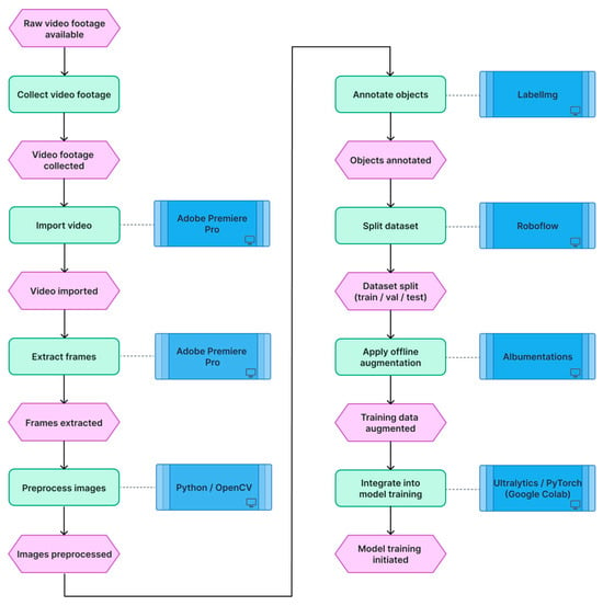
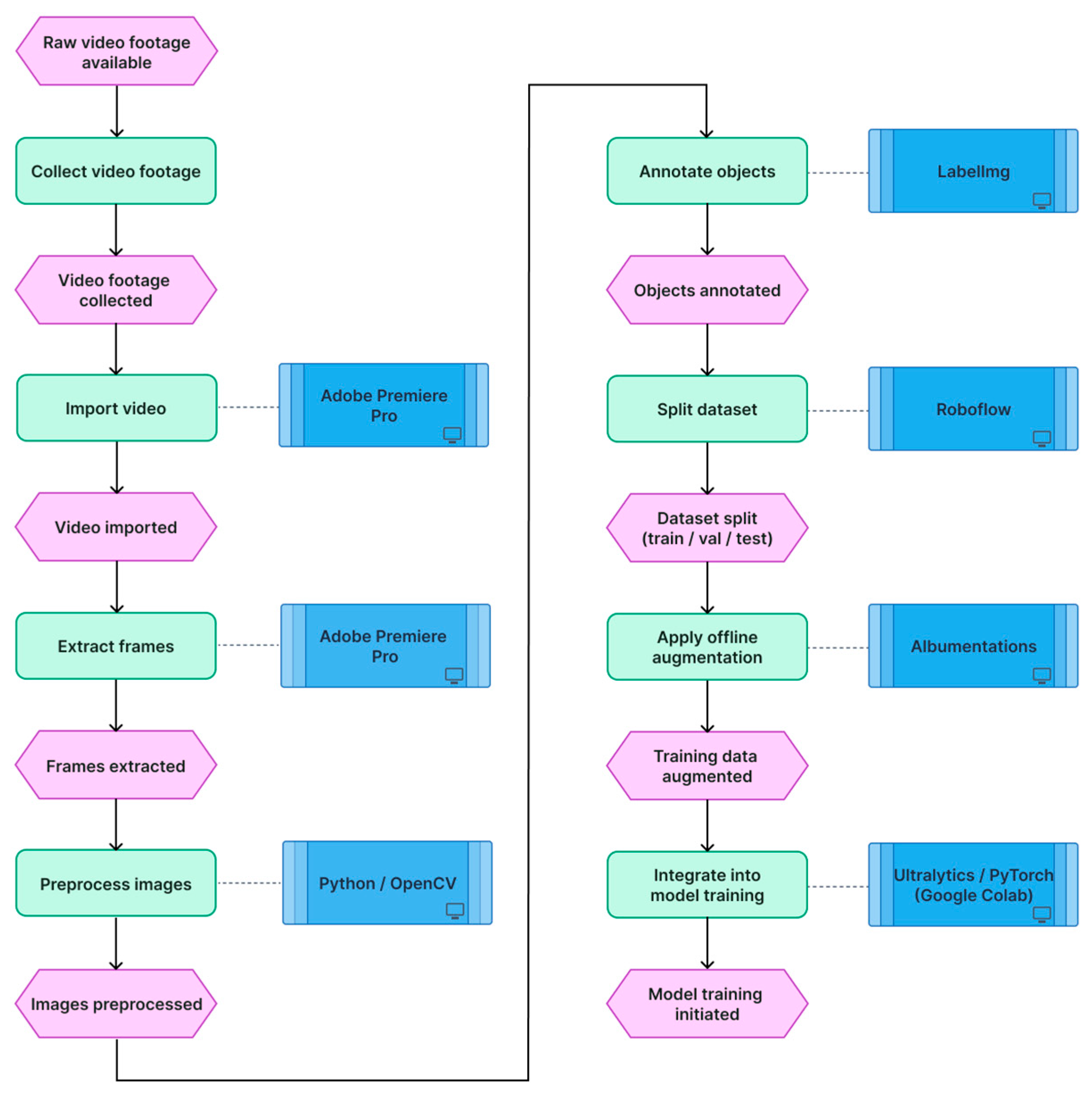
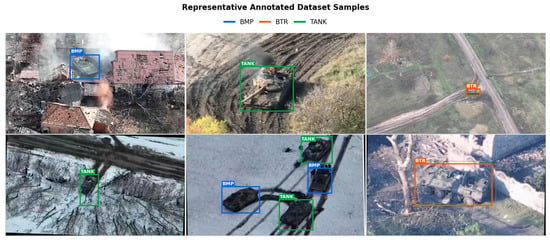
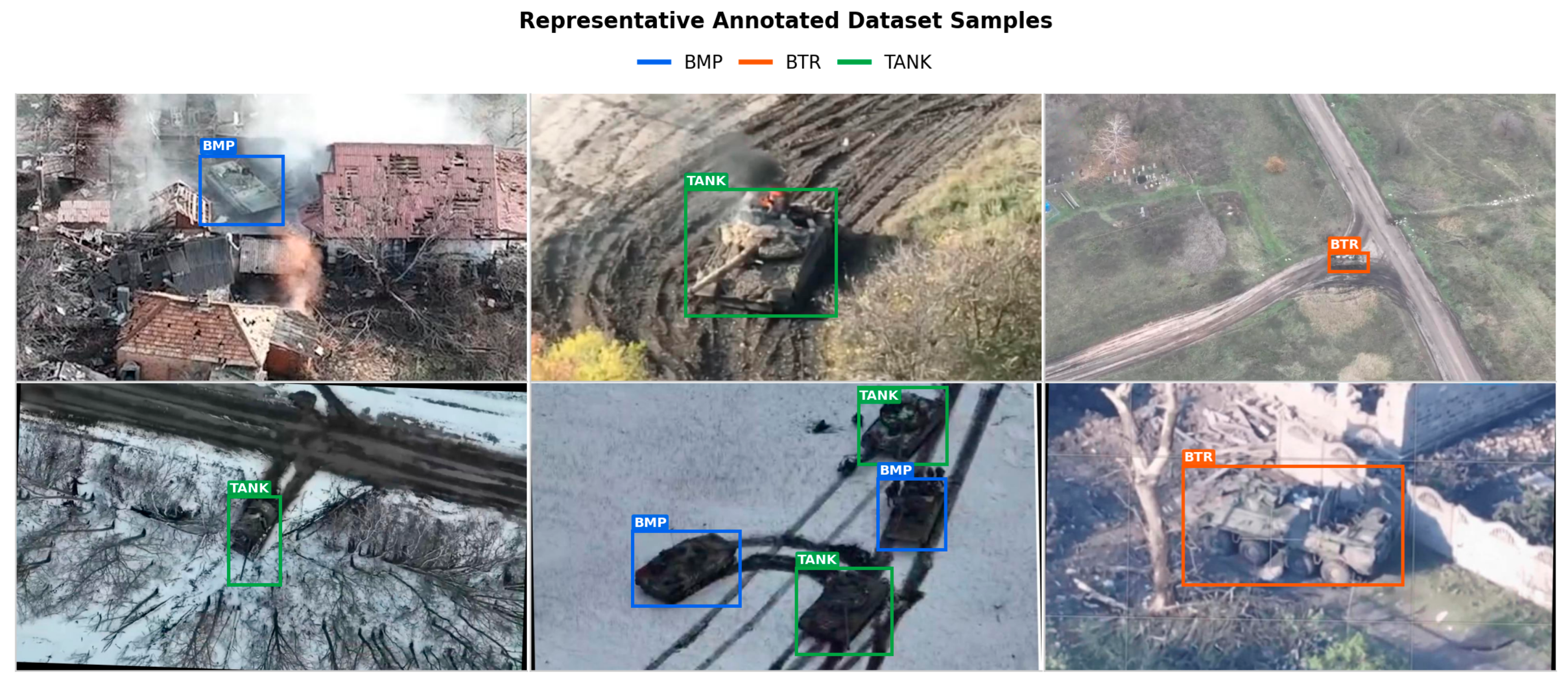
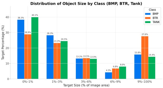
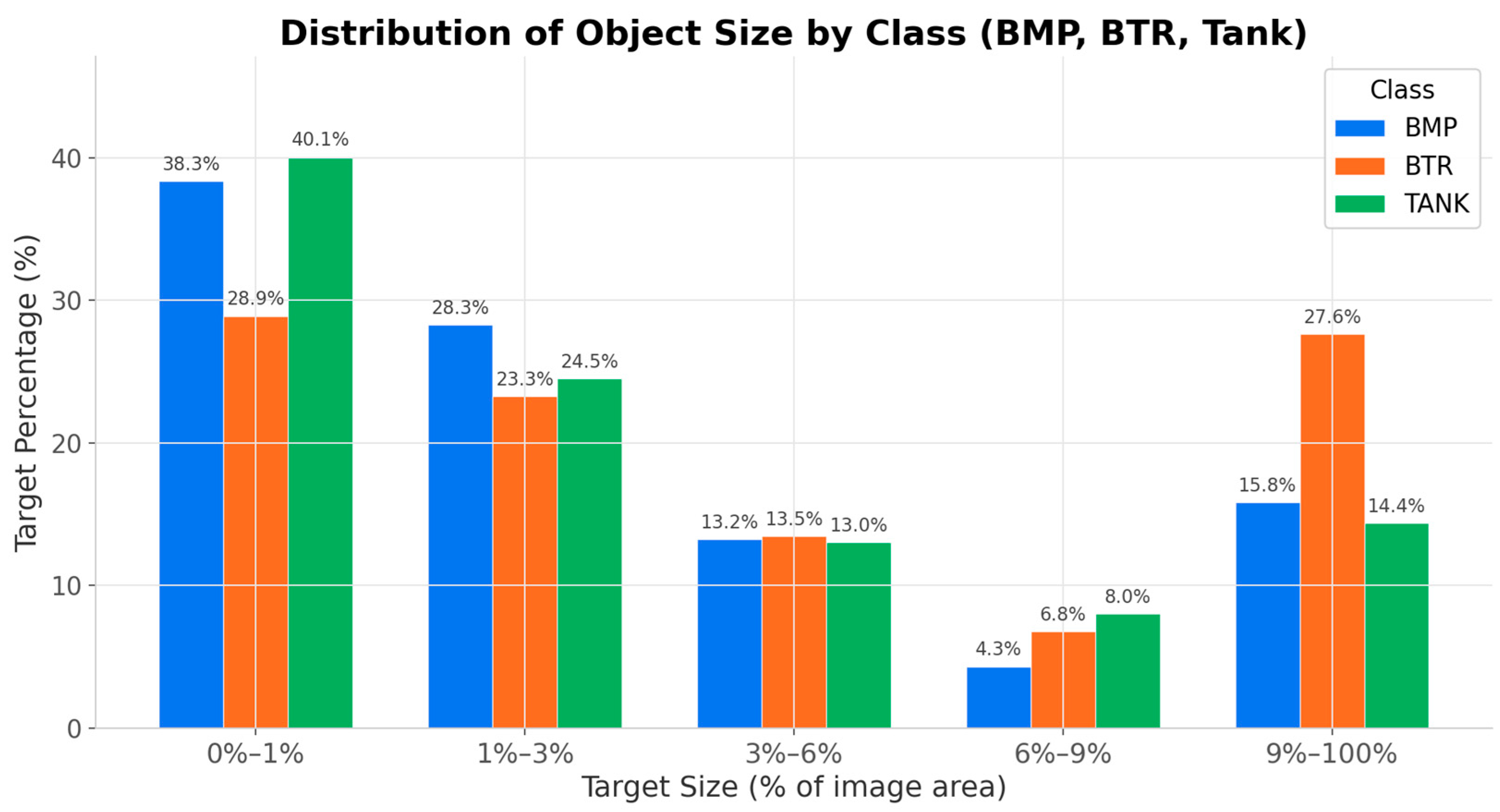
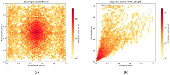
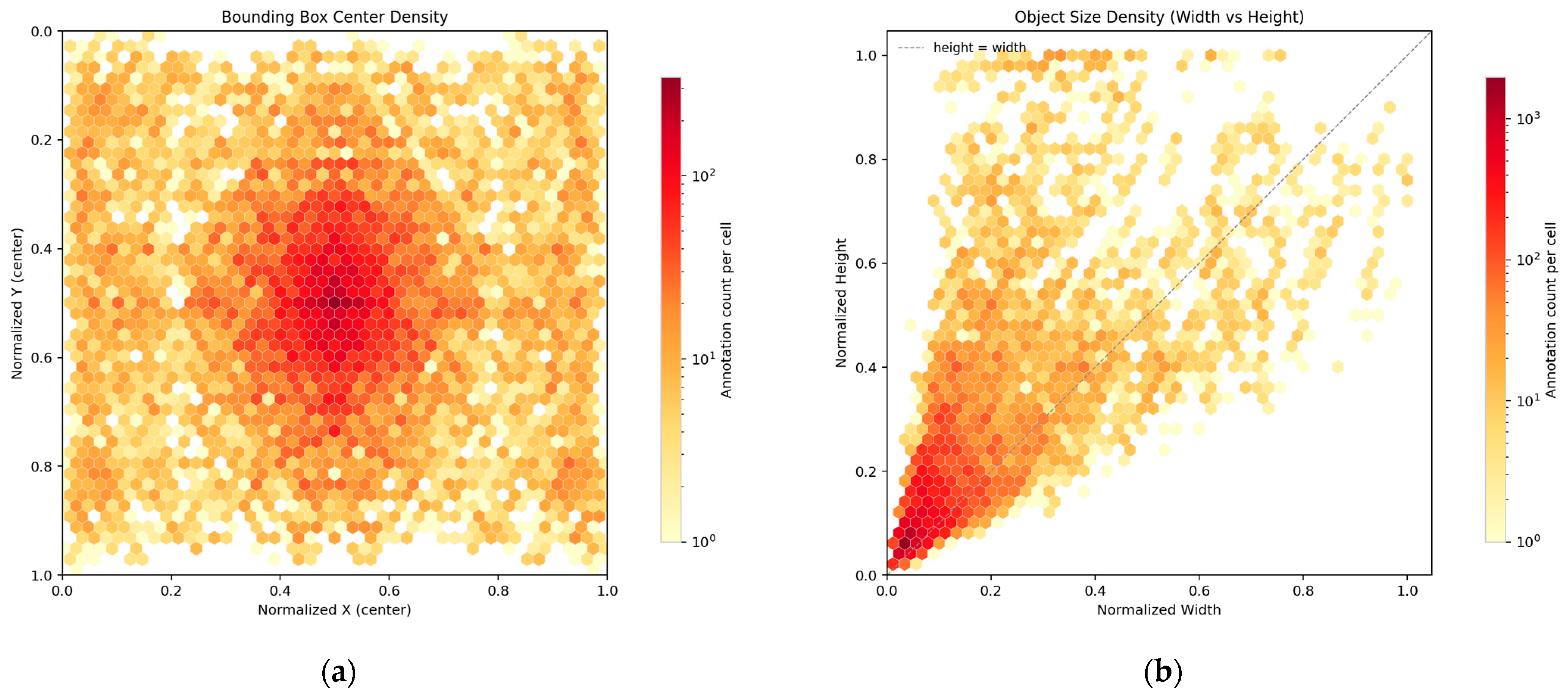
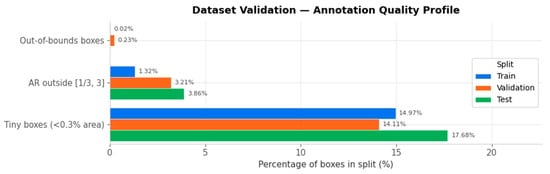
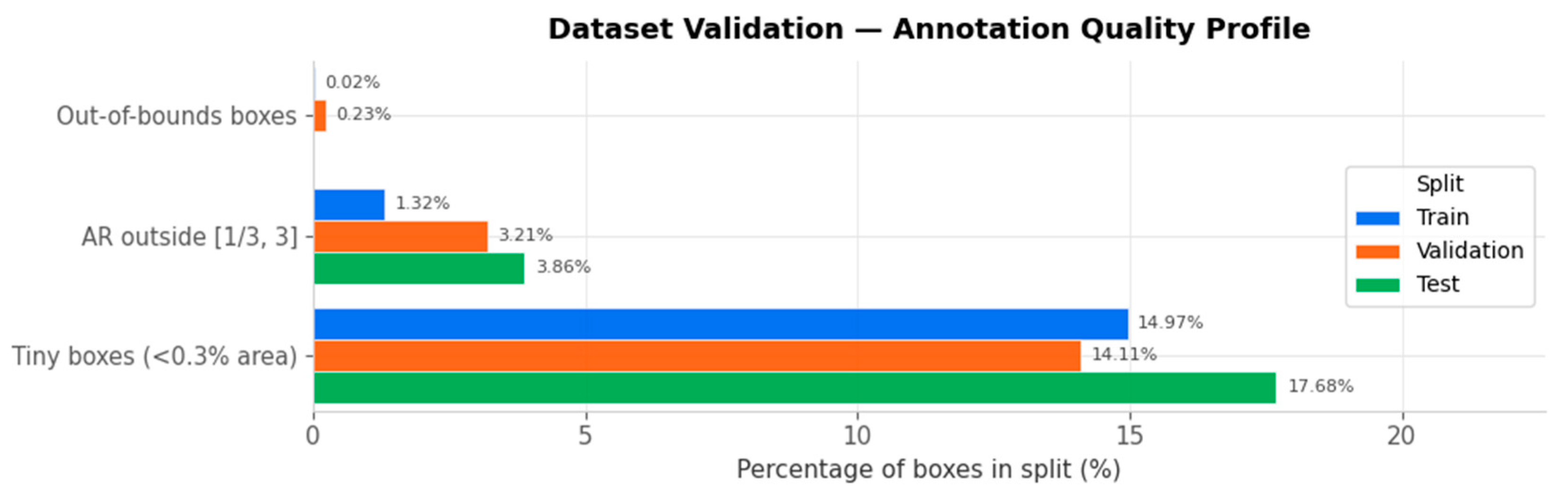
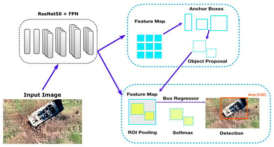
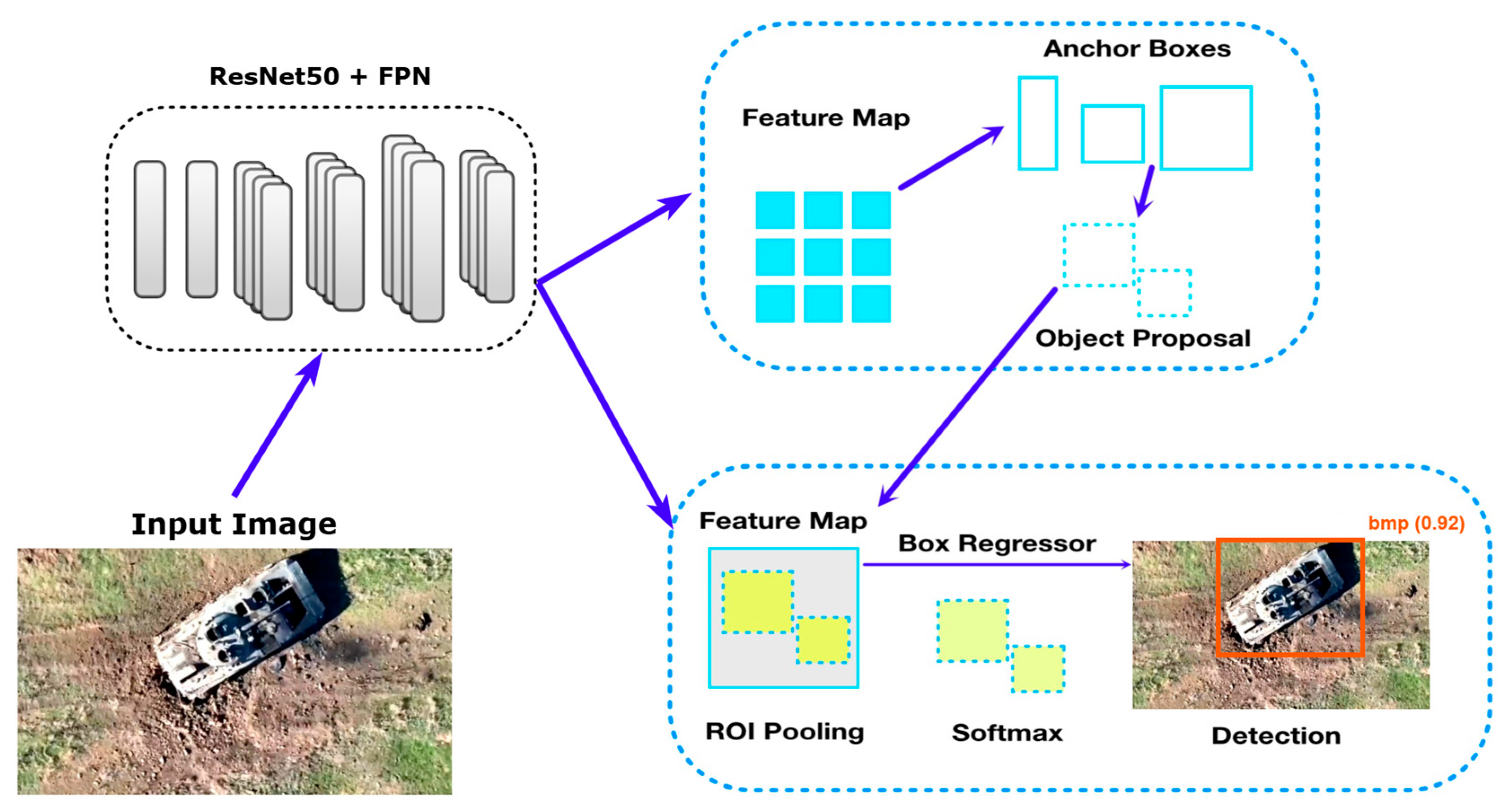
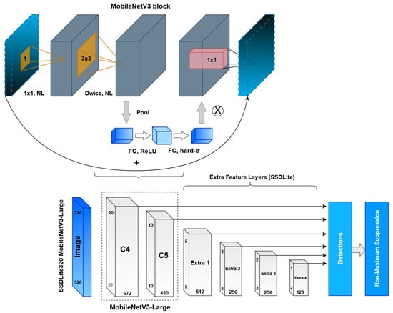
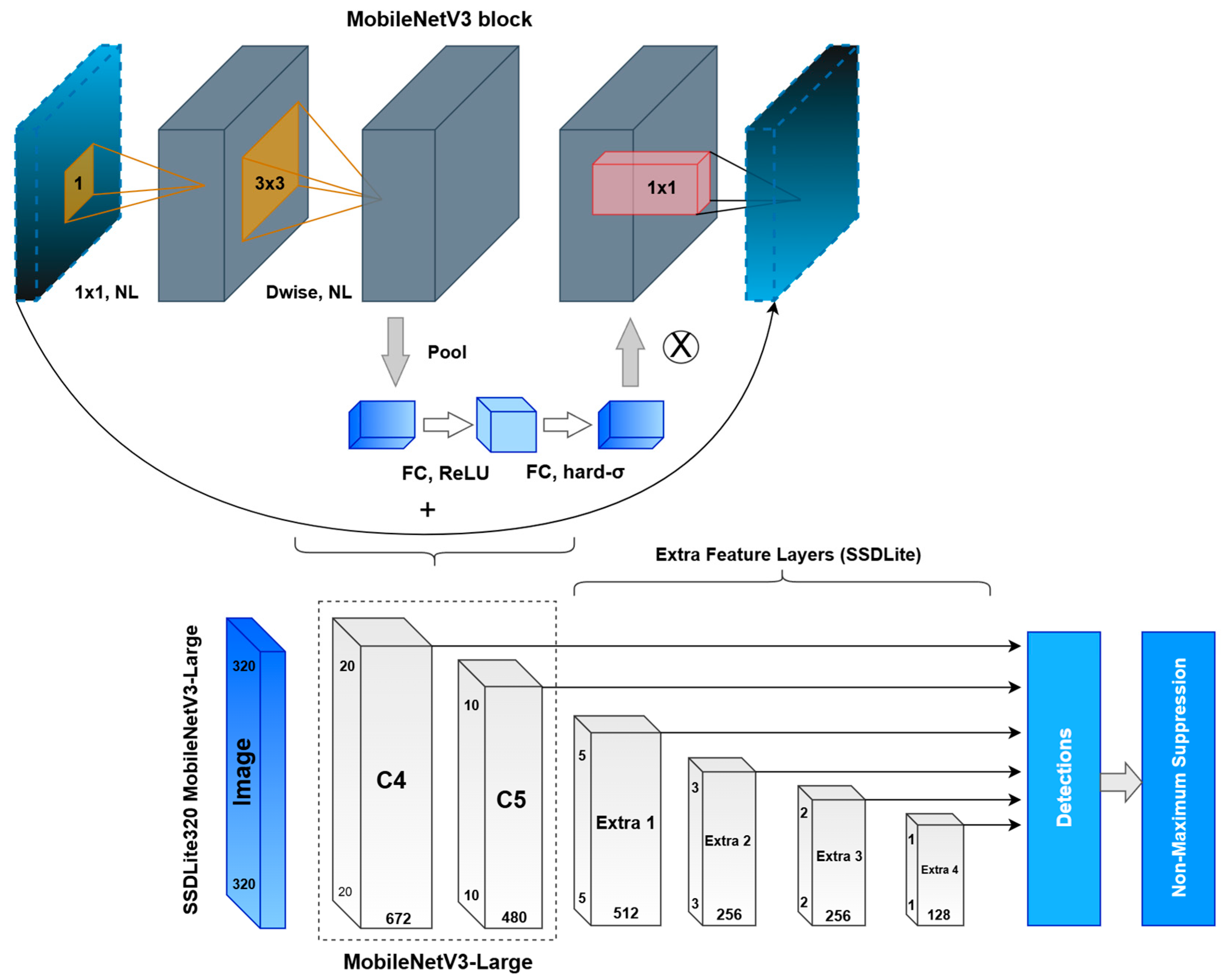
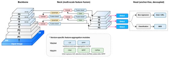
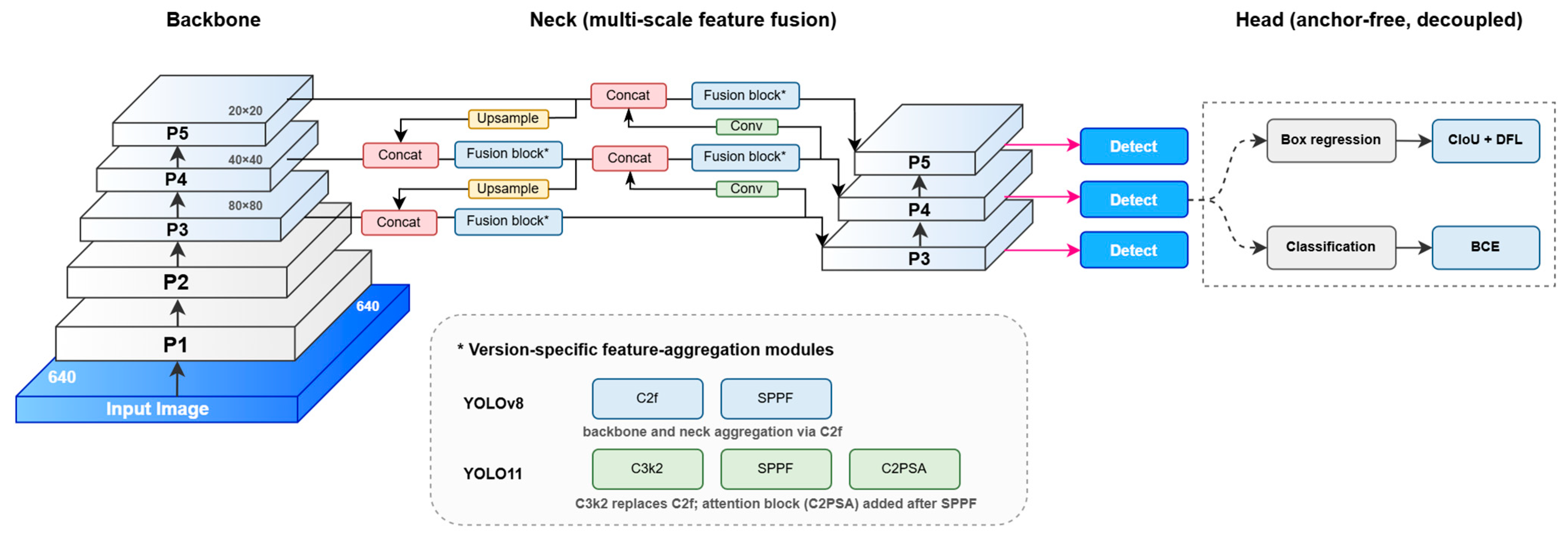
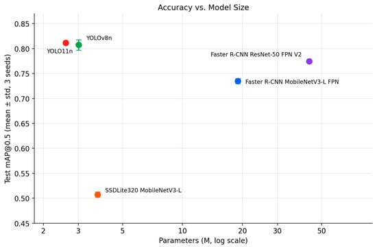
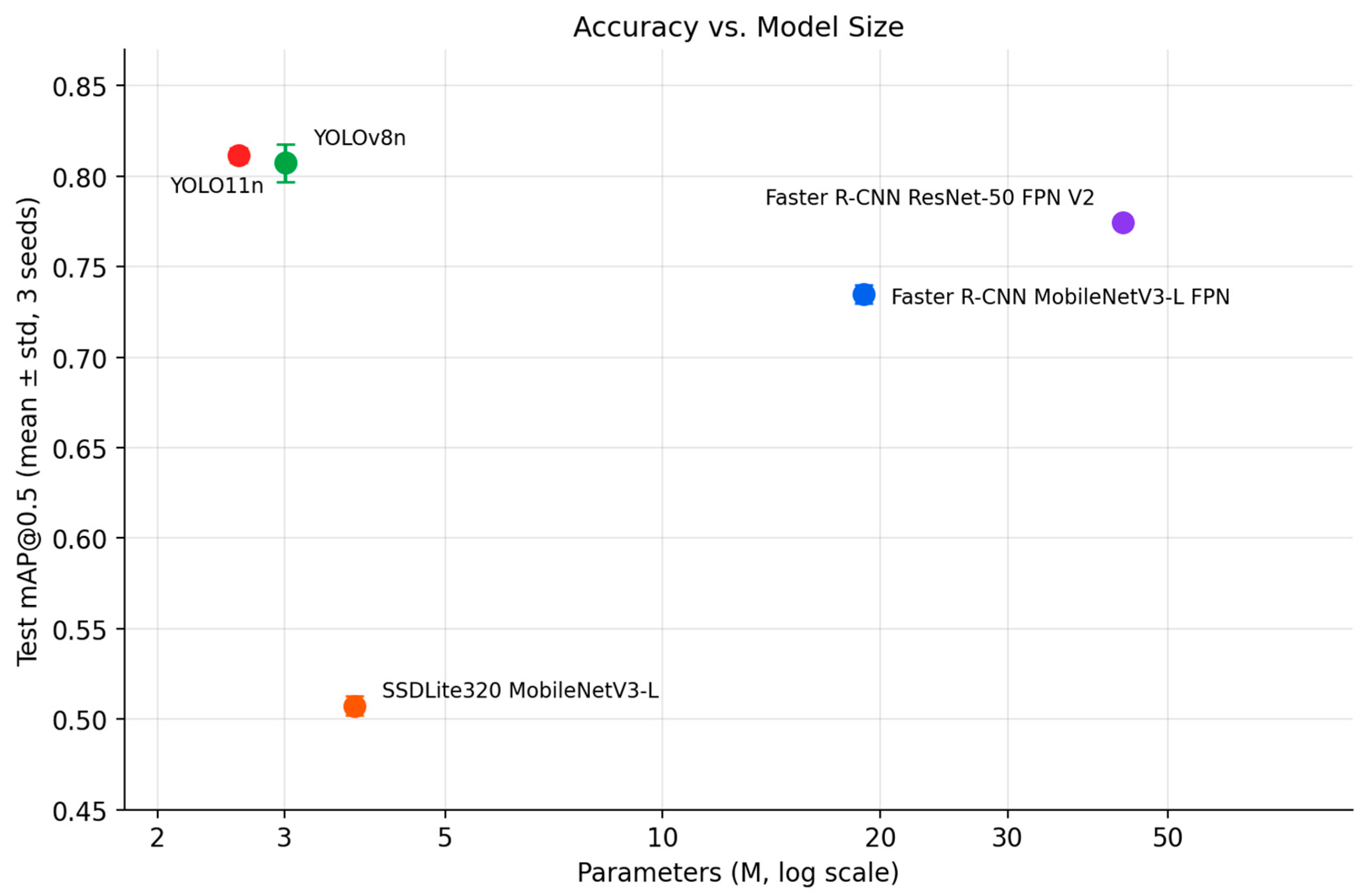
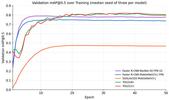
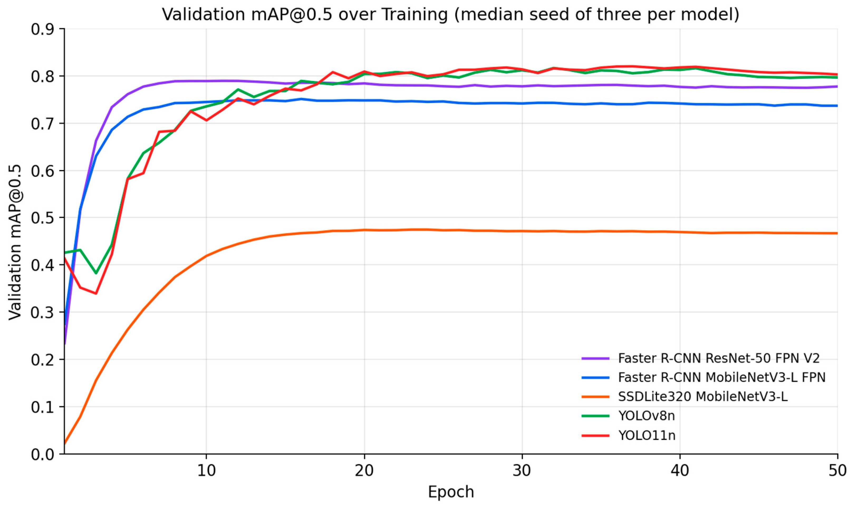
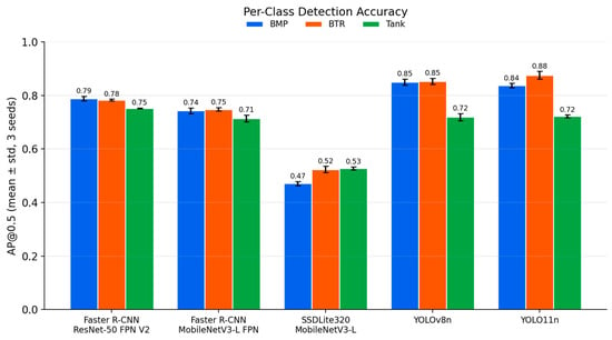
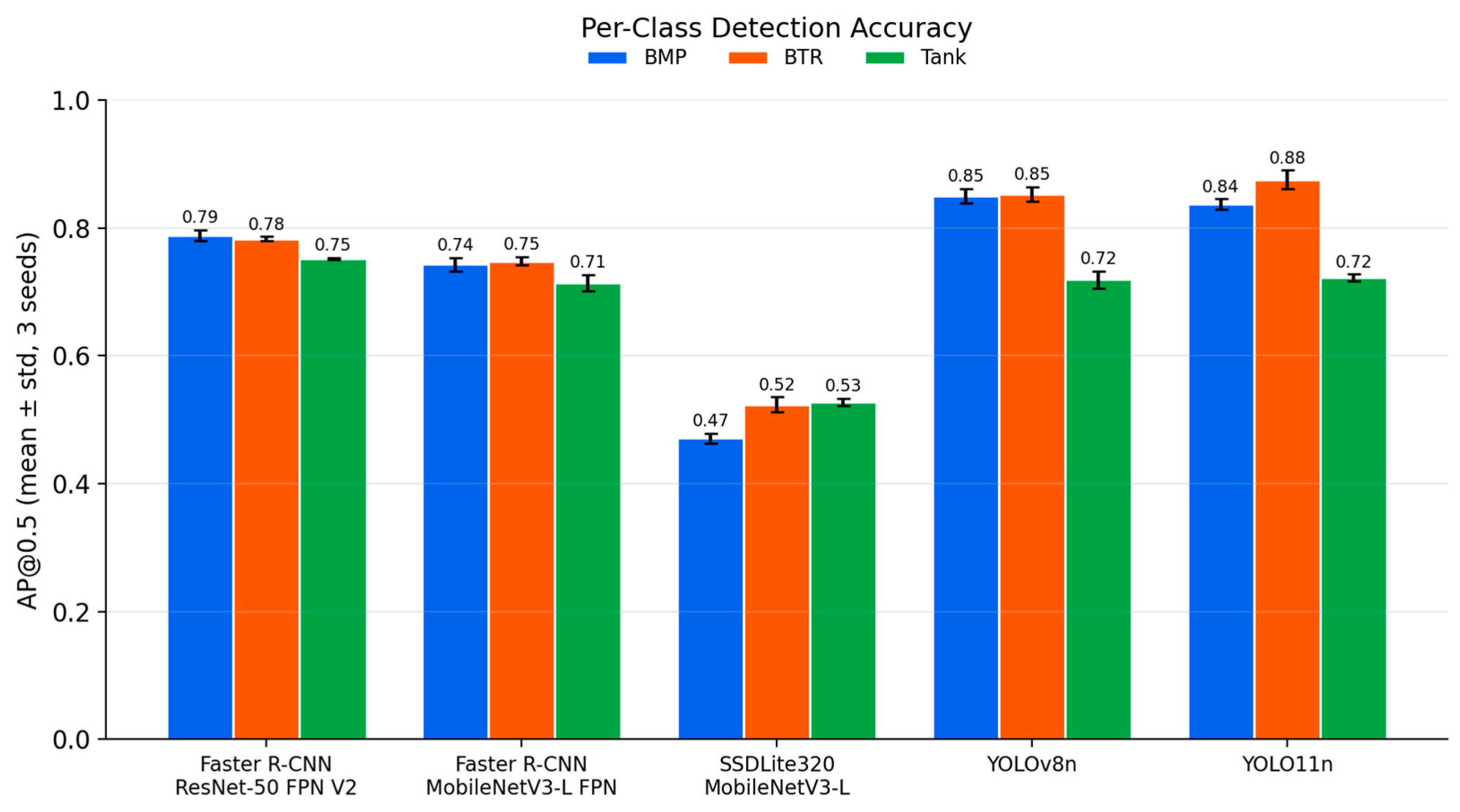
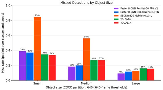
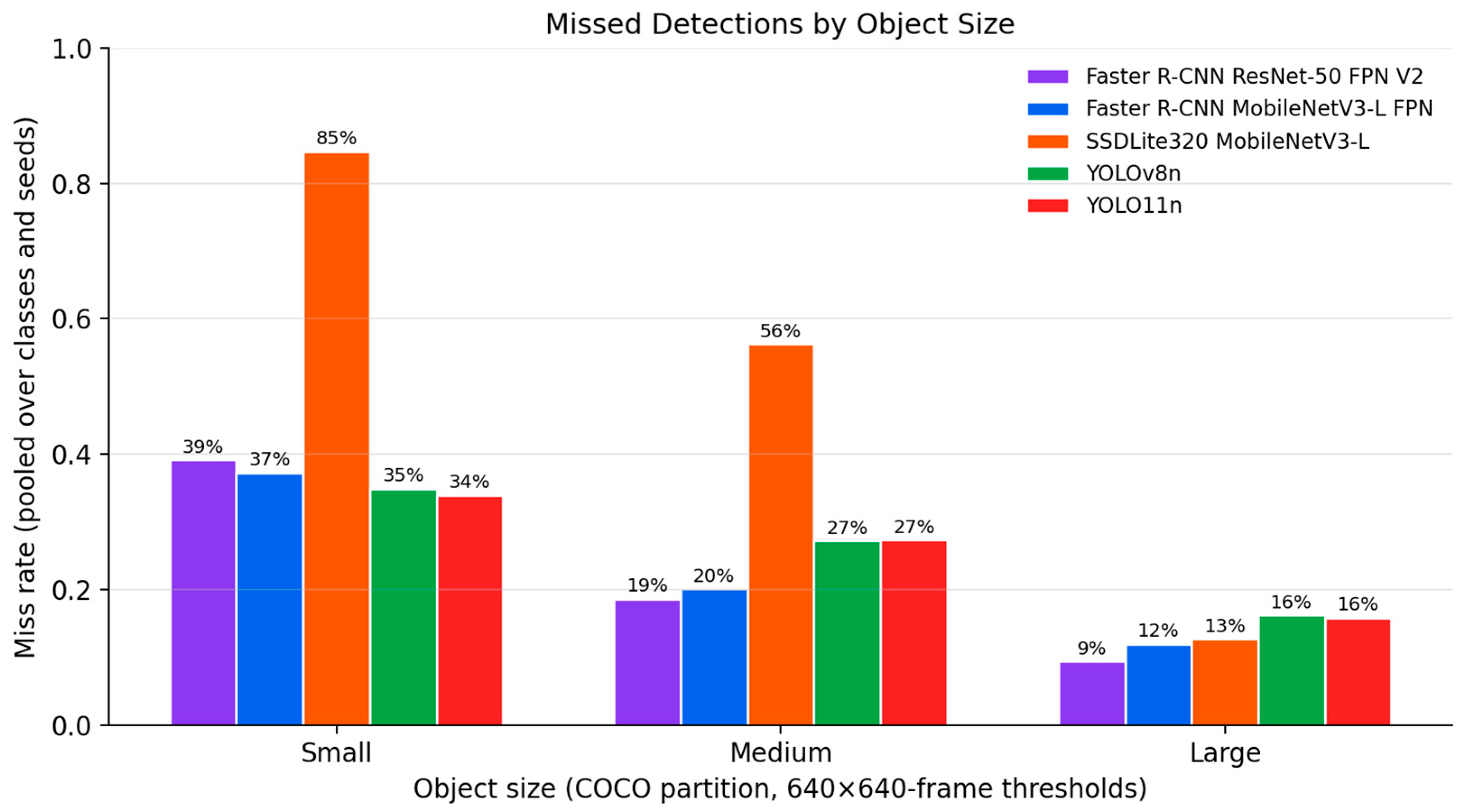
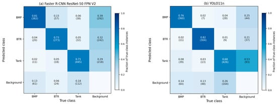
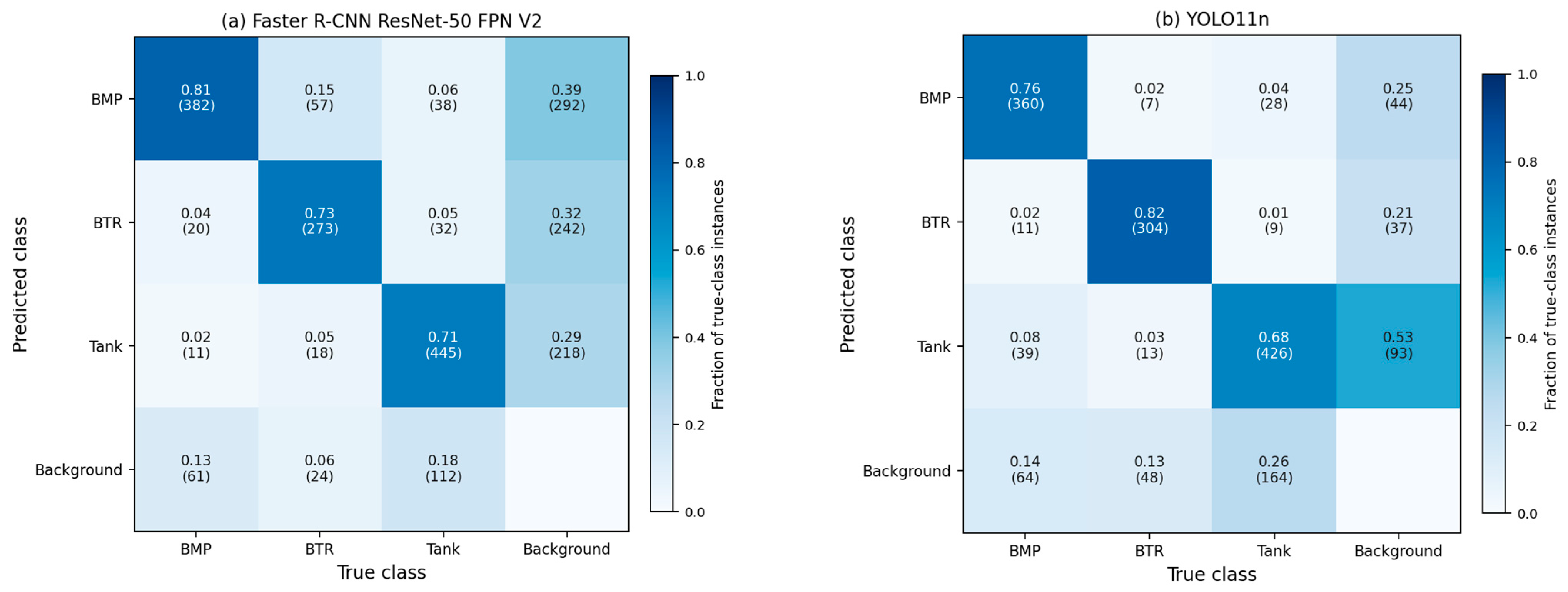
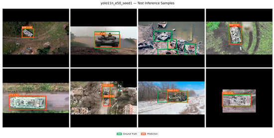
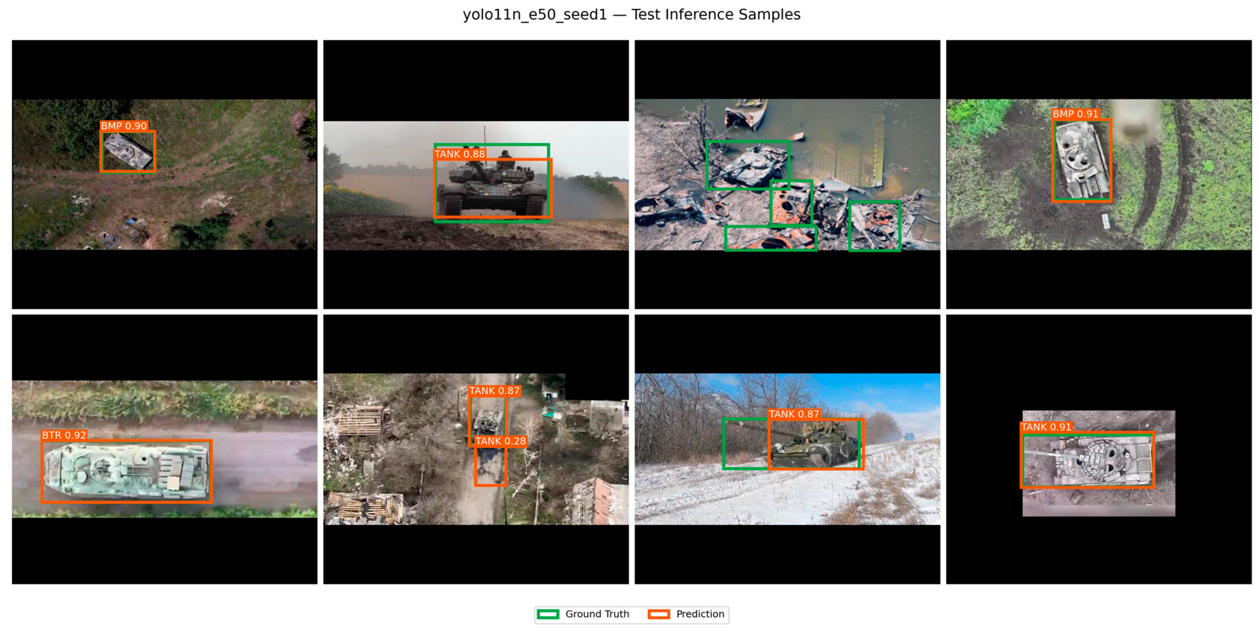
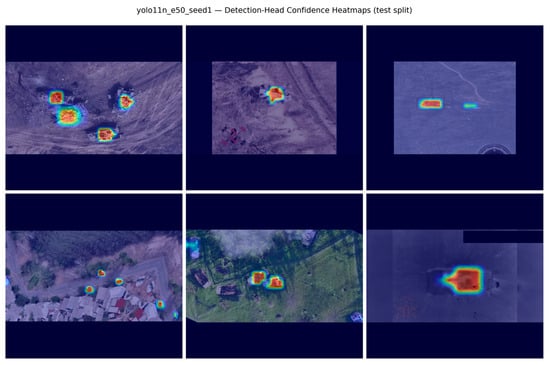
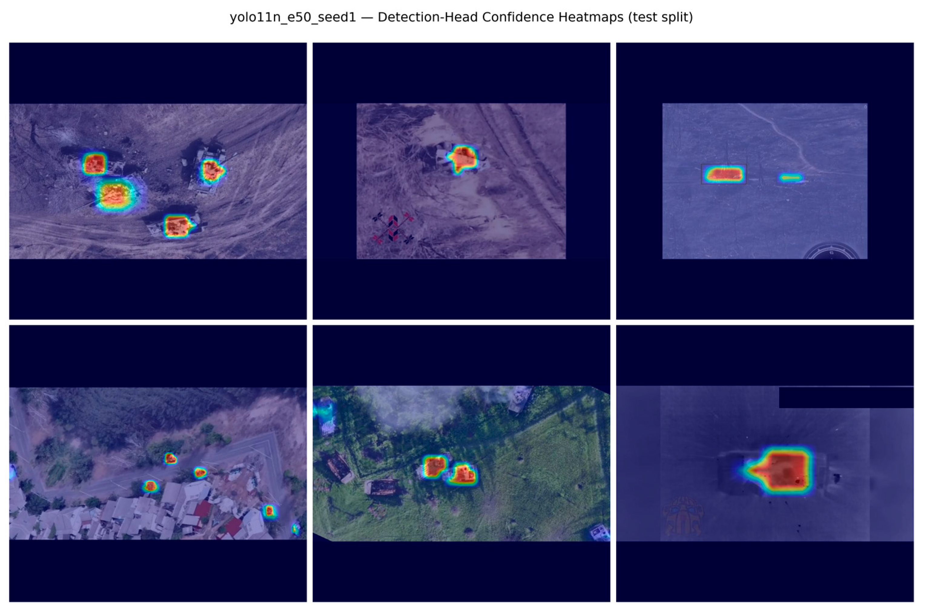
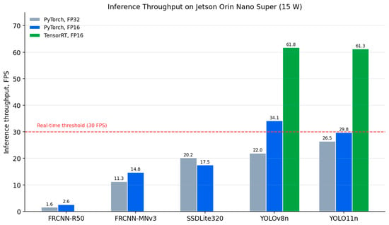
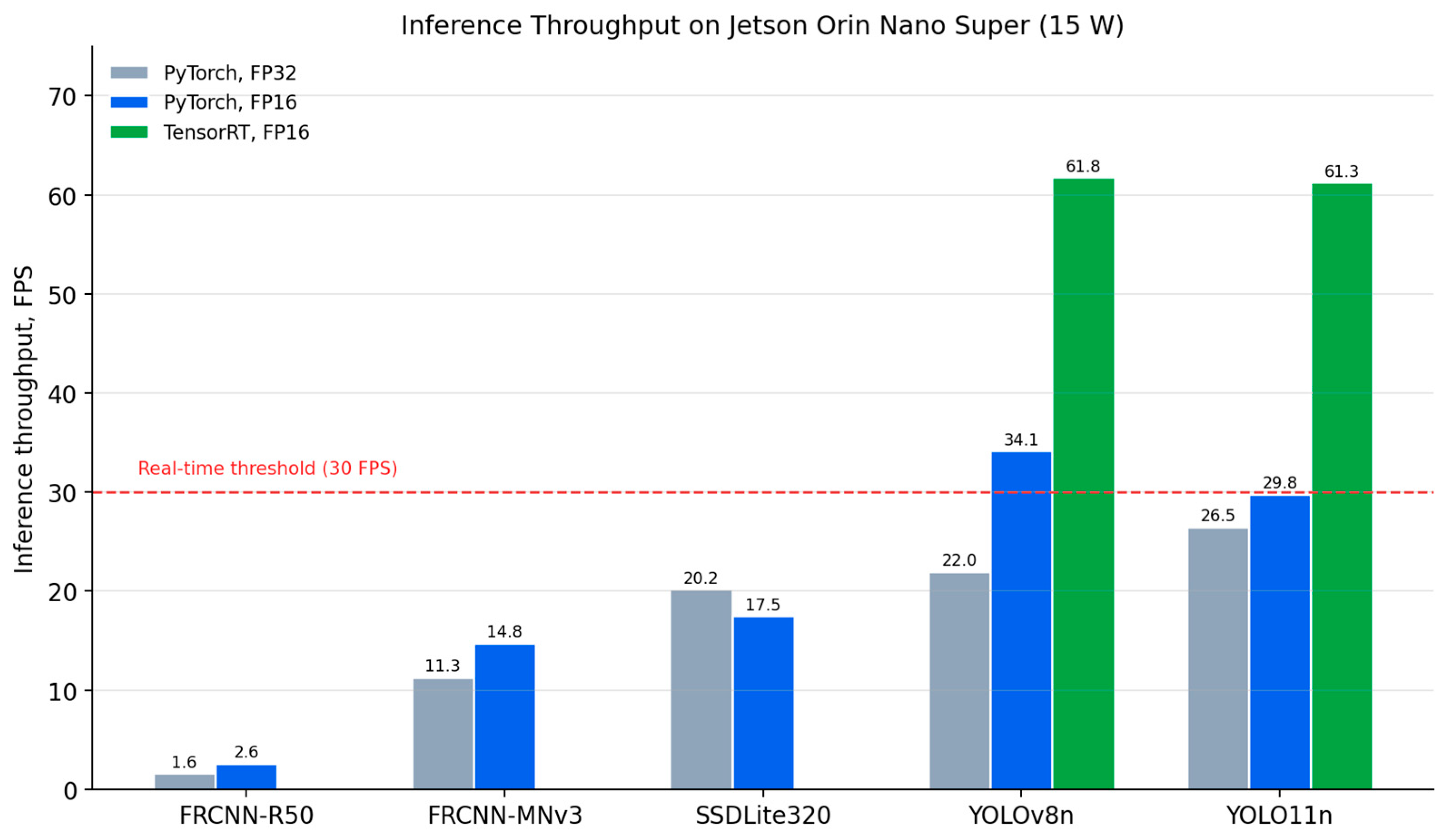
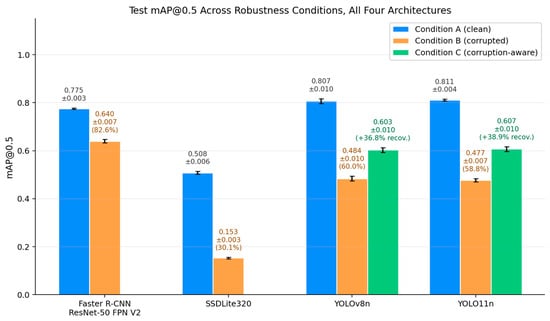
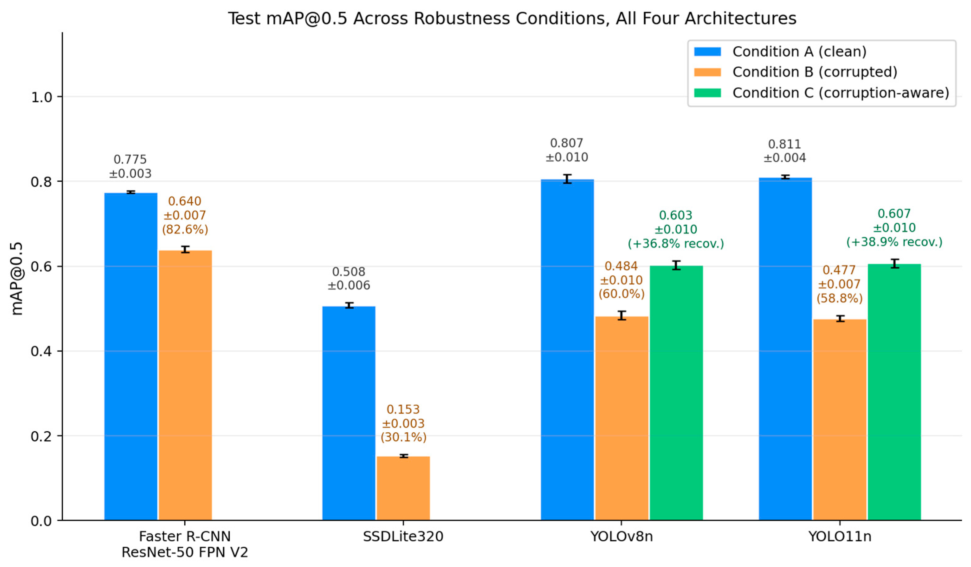
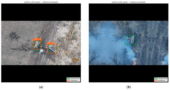
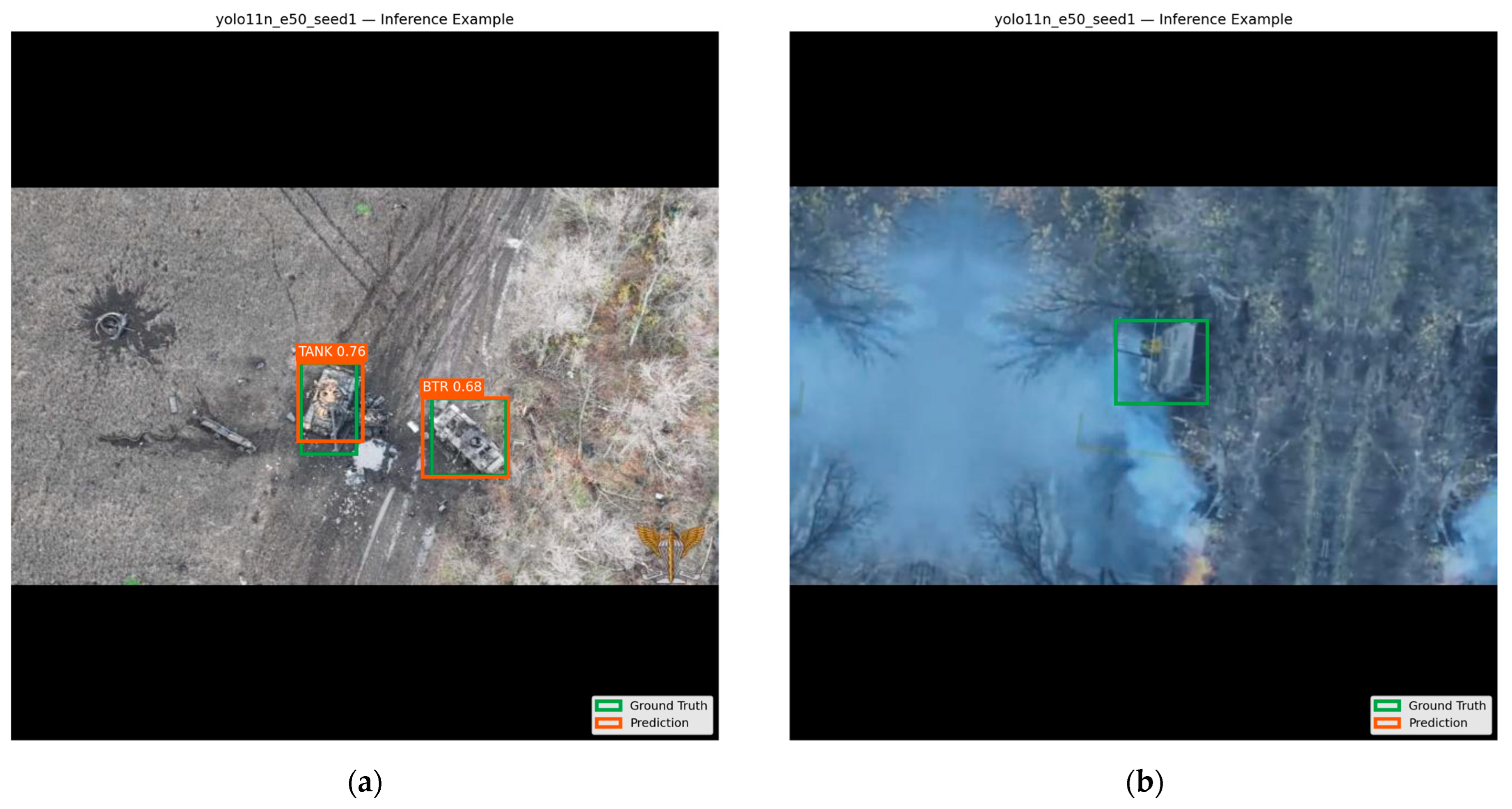

Disclaimer/Publisher’s Note: The statements, opinions and data contained in all publications are solely those of the individual author(s) and contributor(s) and not of MDPI and/or the editor(s). MDPI and/or the editor(s) disclaim responsibility for any injury to people or property resulting from any ideas, methods, instructions or products referred to in the content. |
© 2026 by the authors. Licensee MDPI, Basel, Switzerland. This article is an open access article distributed under the terms and conditions of the Creative Commons Attribution (CC BY) license.