


Abstract
Effective transmission of monetary policy serves as the foundational institutional guarantee for sustaining macroeconomic stability, smoothing cyclical economic fluctuations, and promoting high-quality development. Nevertheless, the underlying determinants driving the time-varying effectiveness of China’s quantity-based monetary policy have not been systematically and empirically delineated in the prevailing literature. This paper first constructs a precise measurement indicator for the effectiveness of China’s quantity-based monetary policy from the output-transmission dimension, which is defined as the response of domestic real output (excluding the contribution of net exports) to orthogonalized exogenous M2 growth shocks. On this basis, the gradient-boosting decision tree (GBDT) model is integrated with the Shapley Additive Explanations (SHAP) framework to quantitatively identify the core determinants that govern the policy effectiveness across different economic cycles and structural transformation stages. The estimation results document clear stage-wise heterogeneity in the drivers of China’s quantity-based monetary policy effectiveness: population-aging and macroeconomic-policy indicators stand out as the dominant explanatory factors over 2002–2008, while economic-structure indicators assume the leading role in shaping policy effectiveness during 2009–2015. The 2016–2022 period is further characterized by the joint dominance of demographic aging and economic-structure dimensions. Within this latest phase, the old-age dependency ratio, real–virtual economy structural misalignment, and distorted aggregate supply configuration exert statistically significant negative marginal contributions to the model-predicted effectiveness of monetary policy, whereas the total fertility rate and potential output growth rate yield positive and economically meaningful contributions.
1. Introduction
Monetary policy is a crucial regulatory tool used by central banks to stabilize the macroeconomy, expand domestic demand, and mitigate risks. The effectiveness of monetary policy depends largely on how smoothly its transmission mechanism operates. This process typically proceeds through multiple stages, from central-bank policy operations and financial-institution behavior to real-economy financing and, ultimately, the investment and consumption expenditures of microeconomic agents. In recent years, amid changes in the external environment, a slowdown in China’s economic growth, insufficient effective domestic demand, and deep-seated structural adjustment, improving the transmission efficiency of China’s monetary policy and strengthening its support for the real economy have become central issues in macroeconomic research and policy practice.
As one of the core instruments in China’s monetary policy regulation framework, quantity-based policy tools have been widely deployed in the policy practices of smoothing business cycle fluctuations and responding to various types of financial shocks (H. Chen et al., 2020). Although factors including the declining stability of money demand and the continuous rise in the endogeneity of money supply have raised academic doubts about the actual effectiveness of quantity-based monetary policy in recent years, quantity-oriented regulation has long occupied a pivotal position in China’s macro policy framework, as evidenced by its historical trajectory of monetary policy operations. A substantial body of empirical studies further confirms that the overall regulatory performance of quantity-based monetary policy still significantly outperforms that of price-based monetary policy in the current Chinese context. Accordingly, combining the salient features of China’s current economic operation, an in-depth investigation into the effectiveness and applicable boundary of quantity-based monetary policy in the dimension of safeguarding financial stability carries important theoretical value and practical policy implications.
Money supply is widely used as an empirical anchor for quantity-based monetary policy in the existing literature (Sheng & Wu, 2009; K. Chen et al., 2018). Its usefulness depends on the extent to which changes in money supply correspond to underlying money demand and support a dynamic balance between supply and demand. However, money demand is embedded in complex microeconomic behavior and macroeconomic conditions and therefore cannot be directly observed with precision. Its determinants also continue to evolve as the financial system develops and shadow banking expands (K. Chen et al., 2018). Clarifying these changes is important for improving the scientific basis of quantity-based monetary policy decisions and the accuracy of policy regulation. The transmission of quantity-based monetary policy generally follows the sequence of “central-bank policy operations–financial-institution behavior–real-economy financing–investment and consumption expenditures.” Frictions at any stage may weaken policy transmission (Choi et al., 2024). Existing studies have examined the factors associated with changes in monetary policy effectiveness from several perspectives. Financial-market conditions may affect the interest-rate, credit, and asset-price channels of monetary policy transmission (C. Liu & Zhang, 2026; X. Tan, 2025). The macroeconomic-policy environment may shape policy expectations and the degree of policy coordination, thereby influencing the realized effects of monetary policy (Caramp & Silva, 2023; Silvo, 2019). Demographic changes may also influence the transmission of monetary policy to the real economy through household saving, consumption propensities, and firms’ investment expectations (X. Chen et al., 2025; Lee, 2026). Although these studies provide an important basis for understanding monetary policy transmission, they mainly examine individual factors or specific mechanisms. Systematic comparisons of the relative importance of multiple factors, their stage-specific variation, contribution directions, and nonlinear relationships remain limited.
Against this background, we examine which indicators are most informative for predicting variations in China’s quantity-based monetary policy effectiveness and how their model-implied associations vary across economic stages. Using the longest common monthly sample from June 2002 to February 2022, we construct a 17-indicator system covering financial markets, macroeconomic policies, economic growth, economic structure, and population aging. We then compare six machine learning regressors, select the best-performing model, and use SHAP values to evaluate predictive importance, contribution direction, and model-implied nonlinear patterns across economic stages.
We make three contributions. First, we develop a two-stage empirical framework designed to characterize the time-varying dynamics of quantity-based monetary policy effectiveness in China. We first use smooth local projections (SLP) to construct a time-varying measure based on the response of domestic real output to exogenous M2 growth shocks. We then compare multiple machine learning models and use SHAP analysis to assess the factors associated with changes in this measure. This approach links the measurement of monetary policy effectiveness with an interpretable analysis of its predictors and allows complex nonlinear relationships to be examined without specifying a single functional form in advance. Second, we construct a system of 17 indicators covering financial markets, macroeconomic policies, economic growth, economic structure, and population aging. The indicators represent the main stages of monetary policy transmission, from central-bank policy guidance and financial institutions’ credit expansion to real-sector activity, firms’ productive investment, and household consumption. This system allows factors located at different stages of the transmission process to be compared within a common framework. Third, rather than relying only on relationships estimated over the full sample, we adopt a stage-specific perspective to examine how the factors associated with quantity-based monetary policy effectiveness evolve as China’s policy environment, economic structure, and demographic conditions change. Applying the same analytical framework to three economic stages makes it possible to compare changes in the relative predictive importance, contribution direction, and nonlinear patterns of the associated factors as China’s policy environment, economic structure, and demographic conditions evolve. This stage-specific approach provides a more dynamic understanding of the factors associated with quantity-based monetary policy effectiveness.
The remainder of this paper is organized as follows. Section 2 reviews the relevant literature and theoretical mechanisms. Section 3 describes the construction of the indicator system, data processing, and sample characteristics. Section 4 measures the output-transmission effectiveness of China’s quantity-based monetary policy and presents analyses of predictive importance and model-implied nonlinear patterns. Section 5 summarizes the main findings and discusses their policy implications.
2. Literature Review
2.1. Measurement of Monetary Policy Effectiveness
Empirical analysis of monetary policy effectiveness first requires a measurable representation of policy effects. Early studies relied mainly on qualitative assessments of policy instruments, transmission channels, and the macroeconomic environment. Although this approach helps clarify the institutional foundations of monetary transmission, it does not quantify the dynamic responses of macroeconomic outcomes to policy shocks. Subsequent research has therefore increasingly adopted structural and time-series models to measure policy effectiveness through estimated output, price, or financial responses.
Dynamic stochastic general equilibrium (DSGE) models evaluate monetary policy effectiveness by tracing macroeconomic responses to policy shocks within a theory-consistent structural framework. Qi et al. (2024) used a DSGE model to examine the effects of debt expansion by real-estate enterprises and households. L. Zhang et al. (2020) employed a time-varying DSGE model to compare quantity-based and price-based monetary policies. Aminu and Nuhu (2025) used a Bayesian DSGE model to evaluate the effects of climate, exchange-rate, and oil-price shocks. These models are well suited to tracing specified transmission mechanisms and conducting structural counterfactual analysis. However, the estimated policy effects depend on the equations, parameter restrictions, and transmission channels imposed by the model. When the objective is to construct a data-driven and continuously updated effectiveness indicator, these structural restrictions may reduce flexibility and increase sensitivity to model specification.
A range of VAR-based models has also been used to evaluate monetary policy effects by estimating the joint dynamics of policy variables and macroeconomic outcomes. Jena et al. (2023) employed a structural vector autoregression model to examine how demographic change affects monetary policy effectiveness. Hauzenberger et al. (2021) used a Bayesian smooth transition VAR model to capture policy effects under different levels of uncertainty. Related nonlinear time-series methods can also allow policy responses to vary across states or directions. One example is the asymmetric autoregressive distributed lag model used by Oyadeyi (2024). These approaches are useful for capturing system-wide dynamics and state dependence. However, VAR estimates can be sensitive to shock-identification assumptions, variable selection, and parameter proliferation. Standard specifications also assume stable underlying relationships unless time variation or regime changes are explicitly incorporated.
Local projections (LP) estimate impulse responses directly at each forecast horizon and impose fewer restrictions on the system’s dynamic structure. Deb et al. (2023) used cross-country LP estimates to examine heterogeneity in monetary policy transmission. X. Chen et al. (2025) applied LP to investigate the effect of population aging on monetary policy effectiveness in China. This flexibility makes LP suitable for tracing policy responses without specifying a complete structural system. However, estimating each horizon separately can produce irregular response paths and relatively high sampling variability, especially when the effective sample is limited. Smooth local projections (SLP) address this limitation by linking response coefficients across horizons through B-spline basis functions and a smoothness penalty (Barnichon & Brownlees, 2019). SLP therefore retains the flexibility and relative robustness of LP while producing more stable and economically interpretable response paths.
2.2. Influencing Factors of Monetary Policy Effectiveness
Monetary policy effectiveness refers to the central bank’s ability to influence output, employment, and prices through instruments such as the money supply and interest rates (Friedman, 1968). Its effectiveness depends on how smoothly policy impulses pass through the transmission mechanism. In China’s institutional setting, this process can be divided into three connected stages. Central-bank operations first guide the balance-sheet decisions and capital allocation of financial institutions. Financial institutions then transmit policy impulses through credit expansion and changes in financing conditions. Finally, firms and households convert the resulting financing into real-sector activity, productive investment, and consumption expenditure. This sequence provides the framework for reviewing the determinants of monetary policy effectiveness.
Macroeconomic-policy factors mainly influence the first two stages through the interest-rate and exchange-rate channels. Monetary policy affects financing costs, aggregate demand, and output by changing market interest rates (Mishkin, 1995). The broader policy environment also influences financial institutions’ balance sheets, risk preferences, and loan pricing. Altavilla et al. (2020) showed that bank capitalization and liability structures affect the pass-through from policy rates to lending rates. Goncharenko and Lukamanova (2025) found that the extent of this pass-through varies across lenders and loan types. X. Zhang and Huang (2024) showed that expansionary policy can stimulate output during low-interest-rate periods by reducing financing costs. Exchange-rate arrangements and external monetary tightening can also affect domestic credit, asset prices, and output (Obstfeld et al., 2017; Ahmed, 2021; Camara, 2025). These studies clarify how policy conditions shape the initial transmission of monetary impulses. However, their focus on individual policies or channels provides limited evidence on the relative importance of downstream financial, structural, and demographic constraints.
Financial-market factors mainly affect the intermediary stage through the asset-price and balance-sheet channels. Policy changes can reprice equity, bond, and foreign-exchange assets, thereby affecting wealth, corporate financing conditions, and market expectations. Gigante et al. (2025) found that financial-market responses to monetary tightening vary across macro-financial conditions. Ngondo and Phiri (2025) identified external policy spillovers through equity, bond, and foreign-exchange markets. Financial institutions’ balance sheets and market liquidity also determine their capacity to absorb and transmit policy shocks. Boutfssi et al. (2026) documented heterogeneous adjustments between policy signals and banking-sector variables. Pessoa and Rochman (2026) showed that non-bank intermediaries and funding liquidity can amplify global financial shocks in emerging markets. This literature explains how policy-induced liquidity is received and redistributed within the financial system. However, it pays less attention to whether this liquidity ultimately supports real-sector activity, productive investment, and consumption expenditure.
Economic growth and economic structure largely determine whether financing is converted into actual expenditure and output at the terminal stage of transmission. Weak growth expectations and low real-sector returns can reduce firms’ willingness to borrow and invest, even when liquidity is abundant. X. Chen and Liu (2025) argued that structural distortions reduce capital returns, potential growth, and entrepreneurial confidence. These conditions weaken the investment response to monetary easing. Imbalances in income distribution and aggregate demand can similarly constrain household consumption capacity and expectations. During economic downturns, reduced policy space and weaker confidence may further prevent liquidity from becoming effective demand (H. Tan et al., 2025). This literature identifies constraints that cannot be captured by examining policy operations and financial intermediation alone. However, growth and structural factors are rarely integrated with upstream policy and financial conditions within a common quantitative framework.
Population aging can affect several stages of transmission through the interest-rate, consumption, and credit channels. Demographic change can alter the natural rate of interest and reduce the scope for conventional interest-rate adjustments. Bielecki et al. (2023) found that demographic transitions increase the likelihood that the zero lower bound becomes binding. Aging also changes household saving and consumption behavior. Kim and Song (2022) showed that retired households respond less strongly to policy shocks than working-age households. Lee (2026) found that aging can shift economic activity toward service sectors that are less sensitive to interest rates. Aging may also reduce real-sector credit demand and alter financial institutions’ risk-taking and credit allocation (Doerr et al., 2024; Leahy & Thapar, 2022). These studies confirm that aging can weaken several links in the transmission mechanism. However, demographic effects are generally examined separately, leaving their importance relative to policy, financial, growth, and structural constraints unresolved.
Methodologically, studies of the determinants of monetary policy effectiveness typically use conventional regressions or structural time-series models to estimate the effects of one or a limited number of factors. These methods are well suited to identifying the direction, magnitude, and statistical significance of prespecified relationships. However, different determinants are usually examined in separate model specifications. Their estimated coefficients are therefore not readily comparable as measures of relative importance. Moreover, incorporating numerous indicators, interactions, and potential nonlinearities into conventional specifications requires the relevant variables and functional forms to be determined in advance. These requirements limit their usefulness for ranking heterogeneous indicators within a unified framework and detecting nonlinear patterns whose forms are not known beforehand.
For this multi-indicator task, machine learning methods provide a complementary analytical framework. They can accommodate multiple predictors, flexibly capture nonlinear relationships and interactions, and generate comparable measures of predictive importance (Varian, 2014; Goulet Coulombe et al., 2022). Recent work has also applied deep-learning architectures to model complex price dynamics in commodity markets (J. He et al., 2026). However, machine learning predictions are often difficult to interpret economically. SHAP addresses this limitation by decomposing model predictions into the contributions of individual features (Lundberg & Lee, 2017). L. Liu et al. (2026) combined a random forest model with SHAP to rank the determinants of China’s monetary policy effectiveness and identify their nonlinear patterns. Extending this approach across multiple machine learning models and economic stages can provide more robust evidence on relative importance, directional contributions, and nonlinear patterns.
2.3. Summary of the Literature
Existing studies provide an important foundation for understanding monetary policy effectiveness, but three related gaps remain. First, the literature has not fully integrated the determinants operating across the principal stages of monetary policy transmission within a unified indicator framework. These stages extend from central-bank guidance and financial institutions’ credit expansion to real-sector activity and the conversion of financing into productive expenditure. Second, the relative importance and directional contributions of multiple determinants have not been systematically compared across different stages of economic development. Third, existing studies have mainly examined linear relationships between individual factors and monetary policy effectiveness, while potential nonlinear relationships have received limited attention. Theoretically, imbalances in economic structure, population aging, and other factors may be associated with monetary policy effectiveness in nonlinear ways. Ignoring these nonlinear patterns may make it difficult to accurately assess the relative importance and contribution directions of different factors.
To address these gaps, we first use SLP to measure China’s quantity-based monetary policy effectiveness through the output response to exogenous M2 growth shocks. We then construct a 17-indicator system covering financial markets, macroeconomic policies, economic growth, economic structure, and population aging. This system connects the principal stages of monetary policy transmission. On this basis, the study compares multiple machine learning models and uses SHAP to examine predictive importance, the direction of contributions to model predictions, and model-implied nonlinear patterns across economic stages.
3. Indicator System and Data
Drawing on the theoretical analysis of the determinants of monetary policy effectiveness and considering data availability, this paper constructs a benchmark indicator system comprising 17 indicators grouped into five categories: financial markets, macroeconomic policies, economic growth, economic structure, and population aging. The details of the indicator system are presented in Table 1.
Table 1.
Description of the indicator system.
3.1. Construction and Definition of the Indicator System
3.1.1. Financial-Market Factors
Financial-market conditions affect monetary policy transmission from central-bank operations to the real economy. This paper selects indicators representing three dimensions: base-money provision, capital-market performance, and cross-border capital flows. First, pledged monetary injection, defined as central-bank liquidity provided through collateral-based lending facilities, is selected to capture changes in the composition of base-money provision. As structural monetary policy tools continue to diversify, the central bank can guide financial institutions to expand credit support for specific sectors through instruments such as relending, thereby affecting monetary policy transmission (Jin et al., 2026). The relevant data are obtained from the People’s Bank of China (PBOC). Second, the Shanghai Composite Index is selected to reflect capital market performance. Fluctuations in stock market prices can affect household wealth, corporate financing conditions, and market expectations, thereby potentially influencing monetary policy effectiveness through the asset-price channel. The relevant data are obtained from the China Economic Information Network (CEI) database. Finally, capital-account openness is selected to reflect restrictions on cross-border capital transactions and the degree of integration between domestic and international financial markets. Greater capital-account openness strengthens linkages between domestic and international financial markets and can affect the independence and effectiveness of monetary policy through exchange-rate expectations and capital flows (Hu, 2020). The relevant data are obtained from the IMF database.
3.1.2. Macroeconomic-Policy Factors
The macroeconomic-policy environment affects monetary policy transmission. This paper selects indicators representing four dimensions: fiscal policy, macroprudential policy, domestic economic policy uncertainty, and U.S. economic policy uncertainty. First, the fiscal policy intensity index is selected to characterize the strength of the fiscal policy stance and its support for aggregate demand. Fiscal and monetary policies jointly influence aggregate demand and economic growth, and the degree of coordination between them affects the effectiveness of macroeconomic stabilization (Chinnakum et al., 2025). The relevant data are obtained from the Macro-Policy Trinity Database. Second, macroprudential policy intensity is selected to characterize changes in the tightening or easing of macroprudential regulation. Macroprudential policy may alter the monetary policy transmission environment by affecting financial institutions’ risk-taking, credit expansion, and stability. Moreover, existing studies show that the effects of monetary and fiscal policy shocks vary under uncertainty (Aye et al., 2019). The relevant data are obtained from the IMF database. Third, the China Economic Policy Uncertainty (EPU) index is selected. Economic policy uncertainty affects corporate investment, household consumption, and the lending behavior of financial institutions, thereby affecting monetary policy effectiveness (Dima et al., 2017). Studies focusing on China also indicate that policy uncertainty can alter the effects of monetary policy on output and technological progress (Zheng & Zhu, 2021) and can exert nonlinear effects on the effectiveness of quantity-based and price-based monetary policies (Song et al., 2021). Finally, the U.S. Economic Policy Uncertainty index is selected. External uncertainty influences domestic monetary policy transmission through capital flows, exchange rate expectations, and financial-market linkages; a high-uncertainty environment typically weakens the effects of monetary policy on the real economy (Aastveit et al., 2017). Furthermore, among major Asian economies, both types of economic policy uncertainty can affect monetary policy effectiveness and generate state-dependent effects (Balcilar et al., 2022).
3.1.3. Economic-Growth Factors
Economic-growth conditions directly affect the real sector’s financing demand and willingness to invest, which in turn determine whether monetary policy can be transmitted smoothly to the output stage. This paper selects indicators across three dimensions: aggregate growth, industrial production, and long-term growth capacity. First, the cumulative year-on-year GDP growth rate is selected to reflect the overall macroeconomic performance. Second, the year-on-year growth rate of industrial value added is selected to capture industrial activity and real-economy conditions. Finally, the potential growth rate is selected to reflect the economy’s long-term sustainable growth capacity. Together, these three indicators characterize the economic-growth environment from the perspectives of demand realization, production activity, and long-term supply capacity. Among them, data for the cumulative year-on-year GDP growth rate and the year-on-year growth rate of industrial value added are sourced from the National Bureau of Statistics (NBS), while data for the potential growth rate are sourced from the Macro-Policy Trinity Database.
3.1.4. Economic-Structure Factors
The state of the economic structure affects the efficiency of monetary policy transmission from the financial system to the real economy. When structural imbalances are substantial, liquidity released by monetary policy may not translate effectively into consumption, investment, and output expansion. This paper selects indicators across four dimensions: aggregate demand structure, income distribution structure, aggregate supply structure, and the real–virtual economy structure. The aggregate demand structure is measured by the ratio of household consumption to GDP to reflect the role of consumption demand in economic growth; the data are sourced from the NBS. The income distribution structure is measured by the wealth Gini coefficient to reflect wealth distribution disparities; the data are sourced from the World Inequality Database (WID). The aggregate supply structure is measured using the contribution rates of human capital and total factor productivity (TFP) to economic growth, which capture the quality and efficiency of the supply side; the relevant data are calculated with reference to the methodology of the Macro-Policy Trinity Database. Following L. Liu et al. (2026), the real–virtual economy structure is proxied by the combined value added of the financial and real-estate sectors as a share of GDP. This measure captures the relative expansion of finance- and asset-related activities within aggregate output, which is relevant to whether liquidity is transmitted to productive investment and consumption or remains concentrated in financial and property markets. The data are obtained from the NBS.
3.1.5. Population-Aging Factors
Demographic structural changes affect household consumption, saving behavior, and credit demand, thereby altering monetary policy transmission. Following L. Liu et al. (2026), this paper incorporates population-aging factors into the indicator system and uses three indicators: the old-age dependency ratio, the total fertility rate, and life expectancy at birth. Specifically, the old-age dependency ratio is used to reflect the elderly-support burden relative to the working-age population; the total fertility rate reflects the prevailing fertility level and long-term population replenishment capacity; and life expectancy at birth captures the longevity dimension of population aging. Together, these indicators characterize demographic change in terms of the old-age support burden, fertility dynamics, and longevity, thereby enabling a more comprehensive analysis of how population aging affects monetary policy effectiveness. The old-age dependency ratio is sourced from the National Bureau of Statistics of China, while the total fertility rate and life expectancy at birth are sourced from the World Bank’s World Development Indicators (WDI) database.
3.2. Data Processing and Sample Description
The SLP estimation uses quarterly data from 2000Q3 to 2024Q1. We subsequently construct the time-varying monetary policy effectiveness measure using three-year rolling windows and convert the resulting quarterly series to a monthly frequency. After accounting for window alignment and the common availability of all 17 predictors, the longest balanced monthly sample for the predictive analysis spans June 2002 to February 2022 (237 monthly observations).
Due to differences in data frequency across indicators, some demographic and economic structural variables are available annually, while certain financial-market and macroeconomic-policy variables are available quarterly. Constructing a consistent monthly dataset follows the mixed-frequency time-series processing approach of Abberger et al. (2023) and applies cubic spline interpolation to convert annual and quarterly variables into monthly observations. Because the candidate algorithms differ in their sensitivity to variable scales, the predictors are standardized within the modeling pipeline for SVM and KNN, using scaling parameters estimated from the training data. The tree-based models are fitted using the original predictor values. Indicator definitions, descriptive statistics, and economic interpretations remain based on the original, unstandardized data. The data files, code, and instructions for reproducing the empirical analysis are provided in the Supplementary Materials.
4. Empirical Results and Analysis
4.1. Measurement of China’s Monetary Policy Effectiveness
We use the exogenous component of M2 growth to identify China’s quantity-based monetary policy shocks and evaluates their effectiveness through the response of domestic real output. Quantity-based instruments operate mainly through the money supply and credit volume, whereas price-based instruments operate through interest rates and exchange rates. China adopted M2 as an intermediate policy target in the late 1990s, and it remained an important gauge of the monetary policy stance (Sheng & Wu, 2009; Fu & Wang, 2020). Interest-rate liberalization has increased the role of price-based and structural instruments and strengthened policy-rate transmission (L. Zhang et al., 2020). Nevertheless, quantity-based instruments remained central throughout much of the sample period (H. Chen et al., 2020; Fu & Wang, 2020; Z. He & Jia, 2020). Although total social financing later became a broader indicator of aggregate credit conditions, M2 retained its historical relevance for identifying quantity-based policy shocks over the period examined. The resulting indicator therefore measures the output-transmission effectiveness of China’s quantity-based monetary policy.
This paper uses the smooth local projections (SLP) method proposed by Barnichon and Brownlees (2019) to measure monetary policy effectiveness. The method introduces B-spline smoothing constraints into the local-projection framework by expressing impulse-response coefficients as smooth functions of the forecast horizon, thereby reducing the large fluctuations in response paths that may arise in conventional local-projection estimates. The model is specified as follows:
where denotes the forecast horizon, and is the real output excluding net exports. Following the approach of L. Liu et al. (2026), this paper selects real GDP excluding net exports to measure the output level. The primary reason is that China’s monetary policy transmission is reflected primarily in its effects on domestic demand, such as consumption and investment, whereas our analysis does not focus on the exchange-rate channel. Therefore, excluding net exports allows the output variable to capture more directly the effects of monetary policy on domestic economic activity. is the monetary policy shock, represents the linear effect of the monetary policy shock, and captures the nonlinear effect associated with the shock size, with used to characterize this nonlinear component. The model controls for the first and second lags of the monetary policy shock, as well as the first and second lags of the output variable.
Here, represents the exogenous component of the monetary policy shock. In this paper, the monetary policy shock refers specifically to the exogenous component of quarterly M2 growth. Because China relied heavily on quantity-based monetary policy for much of the sample period, and quantity indicators such as M2 and total social financing served as important policy signals, this paper adopts the approach of K. Chen et al. (2018) and uses the exogenous component of quarterly M2 growth to measure quantity-based monetary policy shocks. Specifically, the endogenous component of M2 growth is first estimated from monetary policy rules and represents the systematic response of policy authorities to economic conditions. By removing this endogenous component, the exogenous component of quarterly M2 growth is obtained and used as the monetary policy shock variable.
To achieve smooth estimation, this paper expresses the response coefficients at different forecast horizons as linear combinations of B-spline basis functions:
where are the B-spline basis functions, and and are the parameters to be estimated. Under this specification, the monetary policy response coefficients at different forecast horizons are jointly determined by a set of smooth basis functions, thereby producing smoother estimated dynamic response paths.
This cross-horizon regularization reduces the sampling variability that may arise when the response at each horizon is estimated separately, although it may also attenuate highly transitory movements in the response path.
Given the quarterly frequency of the data, we employ a three-year rolling estimation window. Each window contains 12 quarterly observations, within which the smooth dynamic response of output to monetary policy shocks is estimated. The average output response to a medium-sized monetary policy shock is used as an output-response measure of quantity-based monetary policy effectiveness. Let the median of the absolute values of monetary policy shocks within the rolling window be . The effectiveness measure for the m-th rolling window is defined as
where and are the estimated linear and nonlinear response coefficients in the m-th window, respectively. This indicator reflects the average magnitude of the output response to a medium-sized monetary policy shock.
The rolling-window design allows the measure to capture changes in policy transmission over time, although estimates based on local windows may be less precise than those obtained from the full sample.
This output-response measure is informative about the transmission effectiveness of quantity-based monetary policy for three reasons. First, influencing real economic activity is an important objective of monetary policy, and the output response therefore indicates whether monetary impulses are transmitted beyond the financial system to domestic consumption and investment. Second, using the exogenous component of M2 growth reduces the influence of the systematic response of monetary authorities to prevailing economic conditions, allowing the estimated output response to more closely reflect the transmission of quantity-based monetary policy innovations. Third, excluding net exports focuses the measure on domestic real activity, which is more closely related to the consumption and investment channels emphasized in our analysis. A larger positive response indicates stronger output transmission, whereas a response close to zero indicates weak transmission. A negative response indicates that the estimated output effect is adverse or inconsistent with the conventional expansionary transmission mechanism.
Nevertheless, this measure captures only one dimension of monetary policy effectiveness. It does not evaluate the effects of monetary policy on inflation, employment, financial stability, or other policy objectives, nor does it cover price-based or structural monetary policy instruments. Accordingly, the term “quantity-based monetary policy effectiveness” used in this paper refers specifically to the output-transmission effectiveness identified through exogenous M2-growth shocks, rather than to the overall effectiveness of China’s monetary policy framework.
Because the aforementioned SLP model yields a quarterly measure of monetary policy effectiveness, whereas the explanatory variables used in the subsequent analysis are primarily available at a monthly frequency, cubic-spline interpolation is applied to obtain a monthly series covering June 2002 to February 2022. The procedure preserves the values of the original quarterly observations and provides a smooth within-quarter path for frequency alignment. However, the interpolated monthly observations do not contain additional independent economic information, and their within-quarter movements depend on the assumed smooth path. The resulting series is therefore interpreted as a smoothed estimate of the output-transmission effectiveness of quantity-based monetary policy and serves as the dependent variable in the subsequent interpretable machine learning analysis.
To examine whether the factors associated with monetary policy effectiveness vary with the macroeconomic and policy environment, the sample is organized into three institutionally meaningful economic development stages. The 2002–2008 period represents the high-growth stage before the full impact of the global financial crisis. The 2009–2015 period captures post-crisis macroeconomic adjustment, economic recovery, and the transition from high-speed growth toward structural adjustment. The 2016–2022 period corresponds to the advancement of supply-side structural reform and the transition toward high-quality development. This classification reflects major changes in China’s economic development conditions and policy environment and yields sufficiently large, broadly comparable samples for stage-specific machine learning and SHAP analyses.
Within this stage-based framework, Figure 1 shows a broad decline in the output-transmission effectiveness of China’s quantity-based monetary policy. The average response of real output excluding net exports to exogenous M2 growth shocks declined from 0.850 during 2002–2008 to 0.258 during 2009–2015 and then to −0.451 during 2016–2022. The movement from relatively strong positive responses to weaker and eventually negative responses indicates that the transmission environment of quantity-based monetary policy changed substantially across the three economic development stages.
Figure 1.
Evolution of China’s quantity-based monetary policy effectiveness, 2002Q2–2022Q1. Note: The solid line represents the quarterly output-transmission effectiveness of China’s quantity-based monetary policy estimated using smooth local projections with a three-year rolling window. The measure is defined as the average smoothed response of real output excluding net exports to a medium-sized exogenous M2 growth shock. The shaded backgrounds distinguish three economic development stages, 2002–2008, 2009–2015, and 2016–2022, while the gray vertical dashed lines separate these stages. The brown vertical dashed lines and circular markers identify one major event within each stage: the Global Financial Crisis in 2008Q3, the removal of China’s lending-rate floor in 2013Q3, and the initial COVID-19 shock in 2020Q1. The horizontal dashed line denotes zero effectiveness.
4.2. Predictive Analysis of Factors Associated with Monetary Policy Effectiveness
This section examines which indicators are most important for predicting China’s quantity-based monetary policy effectiveness and how their contributions vary across indicator values and economic stages. The 17 indicators cover macroeconomic conditions, financial markets, the policy environment, economic structure and demographic change. Their relationships with monetary policy effectiveness may therefore differ across stages and value ranges. Machine learning models are used to compare predictive performance and identify these patterns.
Based on the above sample, we use machine learning models and SHAP to compare predictive performance and identify the indicators that contribute most to predicting monetary policy effectiveness. First, the dataset is randomly divided into a training set and a test set at a ratio of 7:3, with the random seed set to 30. Six mainstream machine learning algorithms are selected for comparison: support vector regression (SVM), k-nearest-neighbor regression (KNN), gradient-boosting decision tree (GBDT), random forest (RF), LightGBM, and XGBoost. For SVM and KNN, the explanatory variables are standardized before model estimation, whereas the tree-based models are estimated using the original explanatory variables. To enhance model generalization and reduce the risk of overfitting, we use BayesSearchCV for Bayesian hyperparameter optimization. For each model, 100 search iterations are conducted, and five-fold cross-validation is used within the training set to evaluate the predictive performance of different hyperparameter combinations. The cross-validation procedure adopts shuffled KFold cross-validation with five folds and the same random seed of 30. The optimization objective is the negative root mean square error, which is equivalent to minimizing RMSE. After hyperparameter optimization, we evaluate model performance on the test set using R2, RMSE, MAE, MAPE, and shifted MSLE, and select the final model according to the lowest test-set RMSE. The parameter search spaces and optimal hyperparameter values for each model are reported in Table A2 of Appendix A.
Second, the best-performing model is used to calculate SHAP values for all explanatory variables. SHAP decomposes each model prediction into feature-level contributions, allowing the predictive importance and contribution direction of different indicators to be compared on a common scale. Mean absolute SHAP values and SHAP contribution rates are used to rank predictive importance, while the signs of SHAP values indicate whether an observation raises or lowers the model prediction relative to its baseline value. The analysis then compares these predictive contributions across 2002–2008, 2009–2015, and 2016–2022. Finally, following the bin-averaged SHAP approach used by DeMiguel et al. (2023), SHAP dependence plots are employed to examine the model-implied nonlinear contribution patterns of the six predictors with the largest full-sample mean absolute SHAP values. For each predictor, the observations are divided into up to 20 quantile-based bins, and the mean predictor value and mean SHAP value are calculated within each bin. In this study, an empirical turning point is defined as the approximate predictor value at which the binned mean SHAP value changes sign and is estimated by linear interpolation between two adjacent bin means with opposite signs.
The economic interpretation of the SHAP results is anchored in the monetary policy transmission framework developed in Section 2.2. Financial-market and macroeconomic-policy indicators represent conditions at the policy-operation and financial-intermediation stages; economic-growth and economic-structure indicators describe whether financing is converted into real-sector activity, productive investment, and consumption; and population-aging indicators capture demographic conditions that may influence saving, credit demand, and expenditure responses. Within this theoretically organized system, a larger mean absolute SHAP value indicates that an indicator contains more information for predicting variation in the measured output response. It does not measure the causal strength of the corresponding transmission channel. The theoretical framework therefore guides the selection, grouping, and economic interpretation of the predictors, while SHAP provides a common predictive scale for comparing them.
It should be noted that the SHAP analysis in this paper focuses mainly on the main effects and nonlinear marginal contributions of each explanatory variable. Although SHAP dependence plots can provide clues about possible interactions among variables, this paper does not decompose pairwise interaction effects using SHAP interaction values. Therefore, the following analysis interprets the nonlinear patterns as model-implied marginal relationships rather than strict causal interaction effects.
4.2.1. Comparison of Machine Learning Model Performance
Figure 2 shows that all six models achieve strong predictive performance, with the predicted values clustered around the 45-degree line. Compared with the other models, GBDT achieves the highest of 0.8608 and the lowest values for error metrics such as RMSE and MSLE, indicating the best overall predictive performance. Accordingly, after systematic hyperparameter optimization and validation, we select GBDT as the baseline model.
Figure 2.
Comparison of six machine learning models. (a) GBDT. (b) KNN. (c) RF. (d) SVM. (e) XGBoost. (f) LightGBM.
4.2.2. Predictive Importance of Associated Factors
Following the stage classification introduced above, this section compares the predictive importance of the 17 indicators across three economic development stages: 2002–2008, 2009–2015, and 2016–2022. For each stage, mean absolute SHAP values are aggregated into the five indicator categories, and their contribution rates are reported in Table 2. The predictive importance rankings of the individual indicators are presented in Figure 3, Figure 4 and Figure 5. The category-level results show how the importance of broader factor groups changes across stages, while the indicator-level results identify the specific variables that provide the greatest predictive information within each stage.
Table 2.
Contribution rates of the five factor categories across economic stages.
Figure 3.
Stage-specific SHAP predictive importance and contribution distributions, 2002–2008. (a) SHAP contribution rates. (b) SHAP value distribution.
Figure 4.
Stage-specific SHAP predictive importance and contribution distributions, 2009–2015. (a) SHAP contribution rates. (b) SHAP value distribution.
Figure 5.
Stage-specific SHAP predictive importance and contribution distributions, 2016–2022. (a) SHAP contribution rates. (b) SHAP value distribution.
During 2002–2008, population-aging and macroeconomic-policy indicators accounted for 24.82% and 24.68% of total SHAP contributions, respectively. Economic-structure indicators accounted for 22.28%, followed by financial-market indicators at 15.18% and economic-growth indicators at 13.03%. At the individual level, fiscal policy intensity, the old-age dependency ratio, aggregate supply structure, and potential growth rate were the four most important indicators. This pattern is consistent with China’s rapid-growth environment after its accession to the World Trade Organization. Strong external demand, industrial expansion, and infrastructure investment created favorable conditions for credit to be converted into production and expenditure. At the same time, fiscal coordination and demographic-dividend conditions supported labor supply, household income, and investment demand. Policy and demographic indicators therefore provided substantial predictive information about the output response to quantity-based monetary policy.
During 2009–2015, economic-structure indicators became the most important category, with their contribution share rising to 25.70%. Population-aging indicators remained important, accounting for 24.67%, while the contribution share of macroeconomic-policy indicators declined to 19.93%. Aggregate supply structure, potential growth rate, US economic policy uncertainty, and the old-age dependency ratio ranked among the most important individual indicators. This reordering corresponds to the post-crisis adjustment period, when the effects of large-scale stimulus were accompanied by excess capacity, weaker investment returns, and slower potential growth. Under these conditions, the availability of credit alone was less sufficient to generate effective demand. The allocation of financing across sectors and the ability of the supply side to convert credit into productive output therefore became more informative for predicting monetary policy effectiveness.
During 2016–2022, population-aging and economic-structure indicators accounted for 31.88% and 31.83% of total SHAP contributions, respectively, jointly representing 63.71%. Economic-growth indicators accounted for 18.49%, whereas the contribution rates of financial-market and macroeconomic-policy indicators declined to 9.44% and 8.36%. At the individual level, the old-age dependency ratio, real–virtual economy structure, total fertility rate, and aggregate supply structure were the leading indicators. This pattern corresponds to China’s transition towards high-quality development, during which population aging, declining fertility, and slower growth became more pronounced. Meanwhile, the expansion of financial and real-estate activities and continuing supply-side adjustment affected credit allocation, real-sector returns, and financing demand. These conditions help explain why structural and demographic indicators provided more predictive information than policy-related indicators during this stage.
In summary, the predictive hierarchy changed across the three stages. The main sources of predictive information were policy coordination and demographic conditions during the high-growth period, supply-side and structural conditions during the post-crisis adjustment period, and demographic and real–virtual structural conditions during the high-quality development period. This change does not imply that monetary or fiscal policy became irrelevant. Rather, it suggests that the predictive role of policy conditions increasingly depended on whether structural and demographic conditions allowed liquidity to reach productive investment, consumption, and output.
To further examine the directional contribution of each indicator, we analyze the SHAP value distributions shown in Figure 3b, Figure 4b and Figure 5b. Contribution rates primarily reflect predictive importance, whereas the sign of an SHAP value indicates the direction of an observation’s marginal contribution to the model prediction. When high values of an indicator are concentrated in the positive SHAP region, higher values tend to increase predicted monetary policy effectiveness. When they are concentrated in the negative SHAP region, higher values tend to lower predicted effectiveness.
During 2002–2008, high values of fiscal policy intensity, the old-age dependency ratio, aggregate supply structure, and life expectancy were mainly located in the positive SHAP region. These indicators therefore made positive contributions to the model predictions. The positive contribution of fiscal policy intensity is consistent with the role of public expenditure in supporting infrastructure investment and credit demand. Higher potential growth and more favorable supply-side conditions also provided better investment returns, allowing firms to convert credit into production more readily. The positive contribution of the old-age dependency ratio during this period should be interpreted in the context of China’s relatively favorable demographic structure and expanding economy, rather than as evidence that population aging universally improves monetary policy transmission.
During 2009–2015, high values of aggregate supply structure, potential growth rate, US economic policy uncertainty, and the old-age dependency ratio remained mainly in the positive SHAP region. The positive contributions of aggregate supply structure and potential growth rate indicate that the capacity of the real economy to absorb liquidity remained important during the post-crisis adjustment. When growth prospects and production conditions were relatively favorable, credit was more likely to support investment and output. The positive contribution of US economic policy uncertainty may reflect stronger domestic countercyclical policy responses during periods of heightened external uncertainty. By contrast, high values of life expectancy increasingly appeared in the negative SHAP region, suggesting that demographic changes were becoming associated with weaker predicted monetary policy transmission.
During 2016–2022, the contribution directions of several major indicators changed. High values of the old-age dependency ratio, real–virtual economy structure, and aggregate supply structure were concentrated mainly in the negative SHAP region, whereas high values of total fertility rate, cumulative GDP growth, and potential growth rate remained mainly in the positive region. The negative contribution of the old-age dependency ratio is consistent with the possibility that deeper population aging is accompanied by stronger precautionary saving and weaker consumption, credit, and investment demand. The negative contribution of the real–virtual economy structure may indicate that a high concentration of financial and real-estate activity weakens the link between liquidity and productive investment. By contrast, higher fertility and stronger growth conditions are more consistent with stable long-term demand expectations, investment returns, and financing demand.
Overall, the directional SHAP results complement the importance rankings by showing how the contributions of the leading indicators changed across stages. During 2002–2008, fiscal, supply-side, and demographic conditions generally made positive contributions. During 2009–2015, supply-side and growth-related indicators remained positive, while life expectancy began to make a negative contribution. During 2016–2022, the old-age dependency ratio, real–virtual economy structure, and aggregate supply structure made predominantly negative contributions, whereas total fertility rate, cumulative GDP growth, and potential growth rate continued to make positive contributions. This shift is consistent with a transmission environment increasingly shaped by structural and demographic constraints rather than by policy expansion alone.
4.2.3. Nonlinear Contribution Patterns of Key Factors
The importance rankings identify the indicators that provide the most predictive information, but they do not show how the contribution of an indicator changes across its observed value range. Building on the stage-specific importance and directional analysis above, this section uses full-sample SHAP dependence plots to examine the nonlinear contribution patterns of the six indicators with the largest mean absolute SHAP values. Figure 6 presents the relationships for the old-age dependency ratio, aggregate supply structure, real–virtual economy structure, potential growth rate, total fertility rate, and fiscal policy intensity. In these plots, the sign and magnitude of SHAP values show how each indicator contributes to predicted monetary policy effectiveness at different values.
Figure 6.
SHAP dependence plots of six key factors. (a) Old-age dependency ratio (ODR); (b) aggregate supply structure (ASS); (c) real–virtual economy structure (RVS); (d) potential growth rate (PGR); (e) total fertility rate (TFR); and (f) fiscal policy intensity (FPI). The dots represent observation-level SHAP values, and the solid line connects the mean SHAP values calculated within up to 20 quantile-based bins. The dashed vertical lines mark approximate zero-crossing points obtained by linear interpolation between adjacent bins with opposite mean SHAP signs.
Figure 6a shows that the contribution of the old-age dependency ratio changes across several value ranges, with empirical turning points at approximately 12.10%, 13.76%, and 14.64%. When the ratio is below 12.10%, its SHAP values are generally positive. Between 12.10% and 13.76%, they become negative, and between 13.76% and 14.64%, they move back towards zero. Once the ratio exceeds 14.64%, SHAP values become increasingly negative. This pattern indicates that the negative contribution of population aging becomes more pronounced beyond the upper turning point. It is consistent with the possibility that deeper aging is accompanied by greater precautionary saving and weaker debt-financed consumption and investment demand.
Figure 6b shows an empirical turning point of approximately 0.3194 for aggregate supply structure. Below this level, SHAP values are mainly negative, whereas values above 0.3194 are associated with positive SHAP values. This pattern indicates that the contribution of supply-side conditions changes once the indicator reaches a sufficiently favorable range. When productive efficiency and human-capital contributions are limited, additional credit may be less readily translated into real output. Once supply-side conditions improve beyond the turning point, firms may be better able to use available credit for capacity expansion and technological upgrading.
Figure 6c shows a non-monotonic relationship for the real–virtual economy structure, with turning points at approximately 0.0854 and 0.1474. SHAP values are mainly negative below 0.0854, generally positive between 0.0854 and 0.1474, and markedly negative above 0.1474. The intermediate range is therefore associated with a more favorable contribution to predicted monetary policy effectiveness. By contrast, when financial and real-estate activities account for an excessive share of output, liquidity may circulate within asset markets rather than supporting productive real-sector investment, weakening predicted policy transmission.
Figure 6d shows a turning point of approximately 0.0951 for the potential growth rate. Below this value, SHAP values are mainly negative. Above it, they rise into the positive region and remain comparatively high. This pattern indicates that stronger potential growth is associated with a more favorable contribution to predicted effectiveness. Stronger growth prospects may improve expected investment returns, encourage firms to borrow and invest, and make monetary impulses more readily reflected in real output.
Figure 6e shows a turning point of approximately 1.554 for the total fertility rate. Below this level, SHAP values are negative, whereas above it they shift into the positive region. This pattern indicates that a low-fertility environment is associated with a negative contribution to predicted monetary policy effectiveness. Higher fertility may be associated with more favorable long-term demographic expectations and stronger prospective household demand, creating better conditions for monetary liquidity to affect real economic activity.
Figure 6f shows a turning point of approximately 51.44 for fiscal policy intensity. Below this value, SHAP values are mainly negative. Above it, they become positive and follow an upward trend. The result indicates that fiscal support becomes increasingly complementary to predicted monetary policy effectiveness once it exceeds the empirical turning point. Public expenditure may support aggregate demand and credit demand, thereby improving the conditions under which monetary liquidity is converted into real expenditure and output.
Overall, the SHAP dependence plots show that the contributions of the key factors are not constant across their observed value ranges. Aggregate supply structure, potential growth rate, total fertility rate, and fiscal policy intensity make more favorable contributions after entering higher-value ranges. By contrast, the old-age dependency ratio and real–virtual economy structure makes increasingly negative contributions after exceeding their upper turning points. These nonlinear patterns indicate that the output response to quantity-based monetary policy is closely related to the prevailing structural, demographic, and macroeconomic conditions.
4.3. Robustness Checks
To assess the robustness of the baseline empirical findings, we conduct the following robustness checks.
First, the dependent variable is temporally lagged. To mitigate potential endogeneity arising from contemporaneous reverse causality, the explanatory variables in the current period are matched with the monetary policy effectiveness measure six and twelve months later, respectively, while all other model settings remain unchanged. The corresponding results are reported in Appendix A Table A3.
Second, the sample period is adjusted by excluding observations from the period of the major public health emergency. The COVID-19 pandemic in 2020 caused substantial fluctuations in several macroeconomic indicators, which could disproportionately affect the machine learning estimates. Accordingly, all monthly observations from January to December 2020 are removed, and the model is re-estimated using the remaining sample. The corresponding results are reported in Appendix A Table A4.
Third, the original quarterly data are used. To examine whether converting quarterly variables into monthly observations through cubic-spline interpolation materially affects the machine learning results, all variables are aligned at their original quarterly frequency. The GBDT-SHAP analysis is then repeated using the quarterly dataset from 2002Q2 to 2022Q1. The corresponding results are reported in Appendix A Table A5.
Fourth, the machine learning model is replaced. To examine whether the findings depend on the selection of GBDT, the benchmark GBDT model is replaced in turn by support vector regression (SVM), k-nearest-neighbor regression (KNN), random forest (RF), LightGBM, and XGBoost. Each alternative model uses the fixed optimal hyperparameters obtained from the original model comparison, without repeating Bayesian optimization, and the corresponding SHAP values are recalculated. The results for the five alternative models are reported in Appendix A Table A6.
Fifth, time-series validation is conducted. To examine whether the findings depend on the benchmark random train–test split, all observations are arranged chronologically. The earliest 70% of the sample is used for model development, followed by a three-month gap, while the remaining later observations form the final chronological holdout sample. Within the model-development sample, the hyperparameters of the six candidate models are re-optimized using five expanding-window splits, each with a 12-month validation block and a three-month gap. Models are selected according to their mean validation RMSE, and the final holdout sample is not used for model selection. The selected model is then refitted on the full sample, and the stage-specific SHAP contribution rates of the five factor categories are recalculated. The corresponding results are reported in Appendix A Table A7.
Taken together, the four robustness checks provide qualified support for the broad stage-specific pattern identified in the baseline analysis. Economic-structure factors rank first under the six-month specification, whereas economic-growth factors become more prominent under the twelve-month specification. Nevertheless, the combined contribution of financial-market and macroeconomic-policy factors declines from 33.53% to 28.13% and then to 11.20%. After excluding 2020, population-aging factors remain the leading category in the final stage (30.88%). With quarterly data, economic-structure factors instead rank first in the final stage (39.47%); although this differs from the baseline ranking, it preserves the broader shift toward structural factors. Across the five alternative models, the leading final-stage category is consistently either economic structure or population aging. Under the expanding-window time-series validation, the combined contribution of economic-structure and population-aging factors increases from 32.89% to 48.97%, preserving the broader shift toward structural and demographic factors. Thus, the checks support the qualitative robustness of the broad stage-specific evolution, while the exact contribution shares and rankings remain specification-dependent.
The robustness checks above assess the sensitivity of the broad stage-specific patterns to alternative outcome timing, sample composition, data frequency, model choice, and validation design. They do not constitute formal uncertainty intervals for the reported SHAP values, which remain point estimates conditional on the fitted model. Because the dependent variable is constructed from overlapping rolling windows and the monthly observations are serially dependent, conventional bootstrap intervals based on independent resampling would not be appropriate. Future research could quantify SHAP uncertainty through block resampling combined with repeated model refitting.
5. Conclusions and Policy Implications
5.1. Conclusions
We estimate the output-transmission effectiveness of China’s quantity-based monetary policy using quarterly data from 2000Q3 to 2024Q1. It then examines the factors affecting this effectiveness using a corresponding monthly sample of 237 observations from June 2002 to February 2022. After comparing six machine learning models, the study interprets the selected gradient-boosting decision tree (GBDT) model using SHAP. Three main findings emerge.
First, the dominant predictors of China’s quantity-based monetary policy effectiveness shifted from policy-related factors in the early stage to structural and demographic factors in the later stages. During 2002–2008, population-aging and macroeconomic-policy indicators accounted for the largest shares of total SHAP contributions, with fiscal policy intensity, the old-age dependency ratio, aggregate supply structure, and potential growth rate ranking as the most important individual predictors. During 2009–2015, economic-structure indicators became the leading category, while aggregate supply structure and potential growth rate continued to provide substantial predictive information. During 2016–2022, population-aging and economic-structure indicators jointly dominated the prediction of monetary policy effectiveness. Overall, the predictive focus shifted from fiscal-policy coordination and demographic conditions toward economic structure and population aging.
Second, the directional contributions of the leading predictors indicate that structural and demographic constraints became more pronounced in the later stage. During 2002–2008, fiscal policy intensity, the old-age dependency ratio, aggregate supply structure, and life expectancy contributed mainly positively to predicted monetary policy effectiveness. During 2009–2015, aggregate supply structure, potential growth rate, U.S. economic policy uncertainty, and the old-age dependency ratio continued to make predominantly positive contributions, whereas life expectancy contributed negatively. During 2016–2022, the old-age dependency ratio, real–virtual economy structure, and aggregate supply structure made predominantly negative contributions, while the total fertility rate, cumulative GDP growth, and potential growth rate remained positive contributors. These results suggest that population aging and structural imbalances increasingly constrained the predicted output-transmission effectiveness of quantity-based monetary policy.
Third, the key indicators exhibit clear nonlinear threshold patterns in their SHAP contributions. Aggregate supply structure, potential growth rate, total fertility rate, and fiscal policy intensity contributed more positively after exceeding their respective empirical thresholds. In contrast, the contributions of the old-age dependency ratio and real–virtual economy structure became increasingly negative after the indicators exceeded their upper empirical turning points of approximately 14.64% and 0.1474, respectively. These threshold patterns suggest that the output-transmission effectiveness of quantity-based monetary policy is conditional on the economy’s structural quality, demographic profile, growth capacity, and degree of fiscal support.
5.2. Policy Implications
The following implications are conditional on the predictive evidence and distinguish short-run transmission management from longer-run structural adjustment. In the short run, monetary and macroprudential authorities could monitor more closely whether credit and liquidity reach productive activities. The monitoring framework could jointly track credit allocation to manufacturing and small businesses, real-estate financing, leveraged asset transactions, non-bank financial intermediation, and cross-market capital flows. When real-sector credit remains weak while leveraged asset financing expands rapidly, regulators could strengthen loan-use verification and cross-market fund-flow supervision. Targeted reserve requirement reductions, relending, and rediscount facilities could be considered for advanced manufacturing, technological innovation, green industries, and small- and medium-sized enterprises, while differentiated risk weights and capital requirements could be used to limit excessive speculative exposure. The implementation of these measures should be evaluated using indicators such as manufacturing loans, financing costs, private investment, fund-use compliance, and credit risk.
Over the longer term, demographic and structural conditions could be incorporated more explicitly into the design of policy support. In regions experiencing rapid population aging, structural monetary instruments could be evaluated as tools for supporting elderly care, healthcare, age-friendly housing renovation, and inclusive childcare services. Commercial banks could provide medium- and long-term financing whose maturities are better aligned with the cash flows of these service providers. Fiscal authorities could complement these instruments through interest subsidies, guarantee funds, and risk-compensation arrangements. Coordination with pension reform, medical reimbursement, childcare support, and public-service provision could reduce household uncertainty and support consumption demand. These measures should be introduced through regional pilots and evaluated according to credit uptake, investment completion, service consumption, and credit risk before broader implementation.
Across both horizons, a regular coordination mechanism among monetary, fiscal, industrial, and demographic authorities could improve the timing and targeting of the policy mix. When aggregate demand is weak but viable investment projects are available, fiscal authorities could establish project pipelines and provide interest subsidies or credit guarantees, while monetary authorities could provide targeted financing support. When the main constraints arise from technology, equipment, or production capacity, fiscal and industrial policies could prioritize equipment renewal, research and development, digital transformation, and green upgrading, with structural monetary instruments used to reduce financing costs for eligible projects. By contrast, when asset-market leverage and speculative financing are increasing, broad policy expansion should be accompanied by macroprudential safeguards. A pilot–evaluation–adjustment–expansion process could help align short-run transmission objectives with sustainable investment and long-term financial resilience.
Supplementary Materials
The following supporting information can be downloaded at: https://www.mdpi.com/article/10.3390/ijfs14080215/s1, Supplementary Materials: Instructions for Use; source data and code for identifying exogenous M2 growth shocks, smooth local projections, cubic-spline interpolation, model comparison and SHAP analysis, and robustness checks.
Author Contributions
Conceptualization, L.S. and N.J.; methodology, L.S.; software, N.J.; validation, L.S., N.J. and A.W.; formal analysis, N.J.; investigation, N.J.; resources, L.S.; data curation, N.J.; writing—original draft preparation, N.J.; writing—review and editing, L.S., N.J. and A.W.; visualization, N.J.; supervision, L.S. and A.W.; project administration, L.S. and A.W.; funding acquisition, L.S. All authors have read and agreed to the published version of the manuscript.
Funding
This research was funded by the National Social Science Fund of China, grant number 24BTJ002, and the Doctoral Research Start-up Fund of Hubei University of Technology, grant number XJ2023011401.
Institutional Review Board Statement
Not applicable.
Informed Consent Statement
Not applicable.
Data Availability Statement
The datasets generated and analyzed during the current study are available from public sources, including the People’s Bank of China, the National Bureau of Statistics of China, and the Macro-Policy Trinity Database. The processed data supporting the findings of this study are available from the corresponding author upon reasonable request.
Conflicts of Interest
The authors declare no conflicts of interest.
Appendix A
Table A1.
Summary statistics for the variables.
Table A2.
Optimal hyperparameter values obtained from Bayesian optimization.
Table A3.
Robustness results using a lagged dependent variable (%).
Table A4.
Robustness results after excluding the period of the major public health emergency (%).
Table A5.
Robustness results using the original quarterly data (%).
Table A6.
Robustness results using alternative machine learning models (%).
Table A7.
Robustness results using expanding-window time-series validation (%).
References
- Aastveit, K., Natvik, G., & Sola, S. (2017). Economic uncertainty and the effectiveness of monetary policy. Journal of International Money and Finance, 76, 50–67. [Google Scholar] [CrossRef] [Scilit]
- Abberger, K., Graff, M., Müller, O., & Siliverstovs, B. (2023). Imputing monthly values for quarterly time series: An application performed with swiss business cycle data. Journal of Business Cycle Research, 19, 241–273. [Google Scholar] [CrossRef] [Scilit]
- Ahmed, R. (2021). Monetary policy spillovers under intermediate exchange rate regimes. Journal of International Money and Finance, 112, 102342. [Google Scholar] [CrossRef] [Scilit]
- Altavilla, C., Canova, F., & Ciccarelli, M. (2020). Mending the broken link: Heterogeneous bank lending rates and monetary policy pass-through. Journal of Monetary Economics, 110, 81–98. [Google Scholar] [CrossRef] [Scilit]
- Aminu, U., & Nuhu, A. (2025). Monetary policy effectiveness under climate uncertainty: A bayesian dynamic stochastic general equilibrium approach. Asian Economics Letters, 6, 28–34. [Google Scholar] [CrossRef] [Scilit]
- Aye, G. C., Clance, M. W., & Gupta, R. (2019). The effectiveness of monetary and fiscal policy shocks on U.S. inequality: The role of uncertainty. Quality & Quantity, 53, 283–295. [Google Scholar] [CrossRef] [Scilit]
- Baker, S. R., Bloom, N., & Davis, S. J. (2016). Measuring economic policy uncertainty. The Quarterly Journal of Economics, 131, 1593–1636. [Google Scholar] [CrossRef] [Scilit]
- Balcilar, M., Ozdemir, Z. A., Ozdemir, H., Aygun, G., & Wohar, M. E. (2022). Effectiveness of monetary policy under the high and low economic uncertainty states: Evidence from the major Asian economies. Empirical Economics, 63, 1741–1769. [Google Scholar] [CrossRef] [Scilit]
- Barnichon, R., & Brownlees, C. (2019). Impulse response estimation by smooth local projections. The Review of Economics and Statistics, 101, 522–530. [Google Scholar] [CrossRef] [Scilit]
- Bielecki, M., Brzoza-Brzezina, M., & Kolasa, M. (2023). Demographics, monetary policy, and the zero lower bound. Journal of Money, Credit and Banking, 55, 1857–1887. [Google Scholar] [CrossRef] [Scilit]
- Boutfssi, A., Zizi, Y., & Bensouda, M. (2026). Heterogeneous adjustment in monetary transmission: Short-run evidence from an emerging market on bank equity valuations, balance sheets, and inflation. International Journal of Financial Studies, 14, 141. [Google Scholar] [CrossRef] [Scilit]
- Camara, S. (2025). Spillovers of US interest rates: Monetary policy & information effects. Journal of International Economics, 154, 104059. [Google Scholar] [CrossRef] [Scilit]
- Caramp, N., & Silva, D. H. (2023). Fiscal policy and the monetary transmission mechanism. Review of Economic Dynamics, 51, 716–746. [Google Scholar] [CrossRef] [Scilit]
- Chen, H., Funke, M., Losev, I., & Tsang, A. (2020). To guide or not to guide? Quantitative monetary policy tools and macroeconomic dynamics in China. International Journal of Central Banking, 16, 49–94. [Google Scholar]
- Chen, K., Ren, J., & Zha, T. (2018). The nexus of monetary policy and shadow banking in China. American Economic Review, 108, 3891–3936. [Google Scholar] [CrossRef] [Scilit]
- Chen, X., Guo, J., & Zhang, J. (2025). How does aging population affect China’s monetary policy effectiveness: Empirical evidence and theoretical analysis. Economic Modelling, 152, 107309. [Google Scholar] [CrossRef] [Scilit]
- Chen, X., & Liu, Q. (2025). A new explanation for the effectiveness of China’s monetary policy: A new perspective based on macroeconomic structural. Nankai Economic Studies, 8, 104–126. [Google Scholar] [CrossRef]
- Chinnakum, W., Ko, H., Xie, J., Wu, M., & Chaiboonsri, C. (2025). Empirical analysis of economic impact of monetary policy and fiscal policy in china under global uncertainty. International Journal of Financial Studies, 13, 196. [Google Scholar] [CrossRef] [Scilit]
- Choi, S., Willems, T., & Yoo, S. Y. (2024). Revisiting the monetary transmission mechanism through an industry-level differential approach. Journal of Monetary Economics, 145, 103556. [Google Scholar] [CrossRef] [Scilit]
- Deb, P., Estefania-Flores, J., Firat, M., Furceri, D., & Kothari, S. (2023). Monetary policy transmission heterogeneity: Cross-country evidence (Vol. 2023, p. 1). IMF working papers. International Monetary Fund. [Google Scholar] [CrossRef] [Scilit]
- DeMiguel, V., Gil-Bazo, J., Nogales, F. J., & Santos, A. A. P. (2023). Machine learning and fund characteristics help to select mutual funds with positive alpha. Journal of Financial Economics, 150, 103737. [Google Scholar] [CrossRef] [Scilit]
- Dima, B., Dinca, M., Dima, S., & Dinca, G. (2017). Does economic policies uncertainty affect economic activity? Evidences from the United States of America. Romanian Journal of Economic Forecasting, 20, 60–74. [Google Scholar]
- Doerr, S., Kabaş, G., & Ongena, S. (2024). Population aging and bank risk-taking. Journal of Financial and Quantitative Analysis, 59, 3037–3061. [Google Scholar] [CrossRef] [Scilit]
- Friedman, M. M. (1968). The role of monetary policy. American Economic Review, 58, 1–17. [Google Scholar]
- Fu, B., & Wang, B. (2020). The transition of China’s monetary policy regime: Before and after the four trillion RMB stimulus. Economic Modelling, 89, 273–303. [Google Scholar] [CrossRef] [Scilit]
- Gigante, G., Piccolantonio, F., & Scarlini, F. (2025). Monetary policy tightening and financial market reactions: A comparative analysis of soft and hard landings. International Journal of Financial Studies, 13, 150. [Google Scholar] [CrossRef] [Scilit]
- Goncharenko, R., & Lukamanova, E. (2025). Monetary policy pass-through to lending rates: Evidence from the Irish central credit register. Central Bank of Ireland. [Google Scholar]
- Goulet Coulombe, P., Leroux, M., Stevanovic, D., & Surprenant, S. (2022). How is machine learning useful for macroeconomic forecasting? Journal of Applied Econometrics, 37, 920–964. [Google Scholar] [CrossRef] [Scilit]
- Hauzenberger, N., Pfarrhofer, M., & Stelzer, A. (2021). On the effectiveness of the European Central Bank’s conventional and unconventional policies under uncertainty. Journal of Economic Behavior & Organization, 191, 822–845. [Google Scholar] [CrossRef] [Scilit]
- He, J., Xiong, L., & Ning, H. (2026). PDIFormer: Price-discovery-informed deep temporal learning for price dynamics in small-scale commodity markets. Applied Soft Computing, 202, 115841. [Google Scholar] [CrossRef] [Scilit]
- He, Z., & Jia, G. (2020). An institutional analysis of China’s reform of their monetary policy framework. Journal of Economic Issues, 54, 838–854. [Google Scholar] [CrossRef] [Scilit]
- Hu, X. (2020). Can the exchange rate liberalization improve the independence and effectiveness of monetary policy?: Based on the perspective of dual-target and dual-tool policy. World Economy Studies, 5, 45–58+136. [Google Scholar] [CrossRef]
- Huang, Y., & Luk, P. (2019). Measuring economic policy uncertainty in China. China Economic Review, 59, 101367. [Google Scholar] [CrossRef] [Scilit]
- Jena, P. K., Sharma, R., Dehury, T., & Nayak, S. (2023). Impact of monetary policy transmission on the demographic in India: A structural VAR approach. Asian Economics Letters, 4, 77815. [Google Scholar] [CrossRef] [Scilit]
- Jin, L., Li, X., & Zang, J. (2026). Research on the effectiveness of structural monetary policy tools: From the perspective of uncertain risk shock. Reform of Economic System, 3, 114–124. [Google Scholar]
- Kim, M., & Song, S.-y. (2022). The effects of monetary policy on consumption: Workers vs. retirees. Journal of Macroeconomics, 74, 103473. [Google Scholar] [CrossRef] [Scilit]
- Leahy, J. V., & Thapar, A. (2022). Age structure and the impact of monetary policy. American Economic Journal: Macroeconomics, 14, 136–173. [Google Scholar] [CrossRef] [Scilit]
- Lee, J. (2026). Population aging, transition to service economy, and effects of monetary policy. International Journal of Central Banking, 22, 101–144. [Google Scholar]
- Liu, C., & Zhang, T. (2026). The impact of the global financial cycle on the effectiveness of china’s monetary policy. International Economics and Trade Research, 42, 90–107. [Google Scholar] [CrossRef]
- Liu, L., Chen, X., & Chen, Y. (2026). Reassessment of factors affecting the effectiveness of monetary policy: Based on explainable machine learning methods. Journal of Quantitative & Technological Economics, 43, 27–52. [Google Scholar] [CrossRef]
- Lundberg, S. M., & Lee, S.-I. (2017). A unified approach to interpreting model predictions. In Proceedings of the advances in neural information processing systems 30, Long Beach, CA, USA, December 4–9 (pp. 4765–4774). NeurIPS. [Google Scholar]
- Mishkin, F. S. (1995). Symposium on the monetary transmission mechanism. Journal of Economic Perspectives, 9, 3–10. [Google Scholar] [CrossRef] [Scilit]
- Ngondo, M., & Phiri, A. (2025). Has US (Un)conventional monetary policy affected South African financial markets in the aftermath of COVID-19? A quantile–frequency connectedness approach. International Journal of Financial Studies, 13, 153. [Google Scholar] [CrossRef] [Scilit]
- Obstfeld, M., Ostry, J., & Qureshi, M. (2017). A Tie that binds: Revisiting the trilemma in emerging market economies (Vol. 17, p. 1). IMF working papers. International Monetary Fund. [Google Scholar] [CrossRef] [Scilit]
- Oyadeyi, O. O. (2024). Financial development, monetary policy, and the monetary transmission mechanism—An asymmetric ARDL analysis. Economies, 12, 191. [Google Scholar] [CrossRef] [Scilit]
- Pessoa, G. H. R., & Rochman, R. R. (2026). Macro-financial blind spots in emerging markets: Non-bank intermediation, funding liquidity, and the persistence of global shock transmission. International Journal of Financial Studies, 14, 40. [Google Scholar] [CrossRef] [Scilit]
- Qi, Y., Xu, Y., & Tan, H. (2024). Real estate debt expansion and the decline in monetary policy effectiveness: Theory and empirical evidence. Research on Financial and Economic Issues, 11, 46–61. [Google Scholar] [CrossRef]
- Sheng, S., & Wu, P. (2009). The binary transmission mechanism of China’s monetary policy—A research on the “two intermediaries, two targets” model. Frontiers of Economics in China, 4, 335–360. [Google Scholar] [CrossRef] [Scilit]
- Silvo, A. (2019). The interaction of monetary and macroprudential policies. Journal of Money, Credit and Banking, 51, 859–894. [Google Scholar] [CrossRef] [Scilit]
- Song, Y., Yang, Y., Yu, J., & Zhao, Z. (2021). The post-COVID-19 economic policy uncertainty and the effectiveness of monetary policy: Evidence from China. Frontiers in Public Health, 9, 771364. [Google Scholar] [CrossRef] [Scilit] [PubMed]
- Tan, H., Chen, X., & Chen, Y. (2025). Does the narrowing of monetary policy space weaken monetary policy effectiveness? Journal of Finance and Economics, 51, 123–137. [Google Scholar] [CrossRef]
- Tan, X. (2025). The effectiveness of China’s interest rate channel of monetary policy transmission: Evidence from external instruments VAR. Journal of Applied Statistics and Management, 44, 348–360. [Google Scholar] [CrossRef]
- Varian, H. R. (2014). Big data: New tricks for econometrics. Journal of Economic Perspectives, 28, 3–28. [Google Scholar] [CrossRef] [Scilit]
- Zhang, L., Yin, H., & Wang, Q. (2020). Quantity type or price type—Empirical evidence from the “Non-Linear” effectiveness of monetary policy. China Industrial Economics, 7, 61–79. [Google Scholar] [CrossRef]
- Zhang, X., & Huang, Q. (2024). “A Drop in the Ocean” or “Offer Fuel in Snowy Weather”—Research on the effectiveness of monetary policy in a low interest rate environment. South China Journal of Economics, 5, 75–94. [Google Scholar] [CrossRef]
- Zheng, G., & Zhu, S. (2021). Research on the effectiveness of China’s macro control policy on output and technological progress under economic policy uncertainty. Sustainability, 13, 6844. [Google Scholar] [CrossRef] [Scilit]
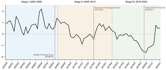
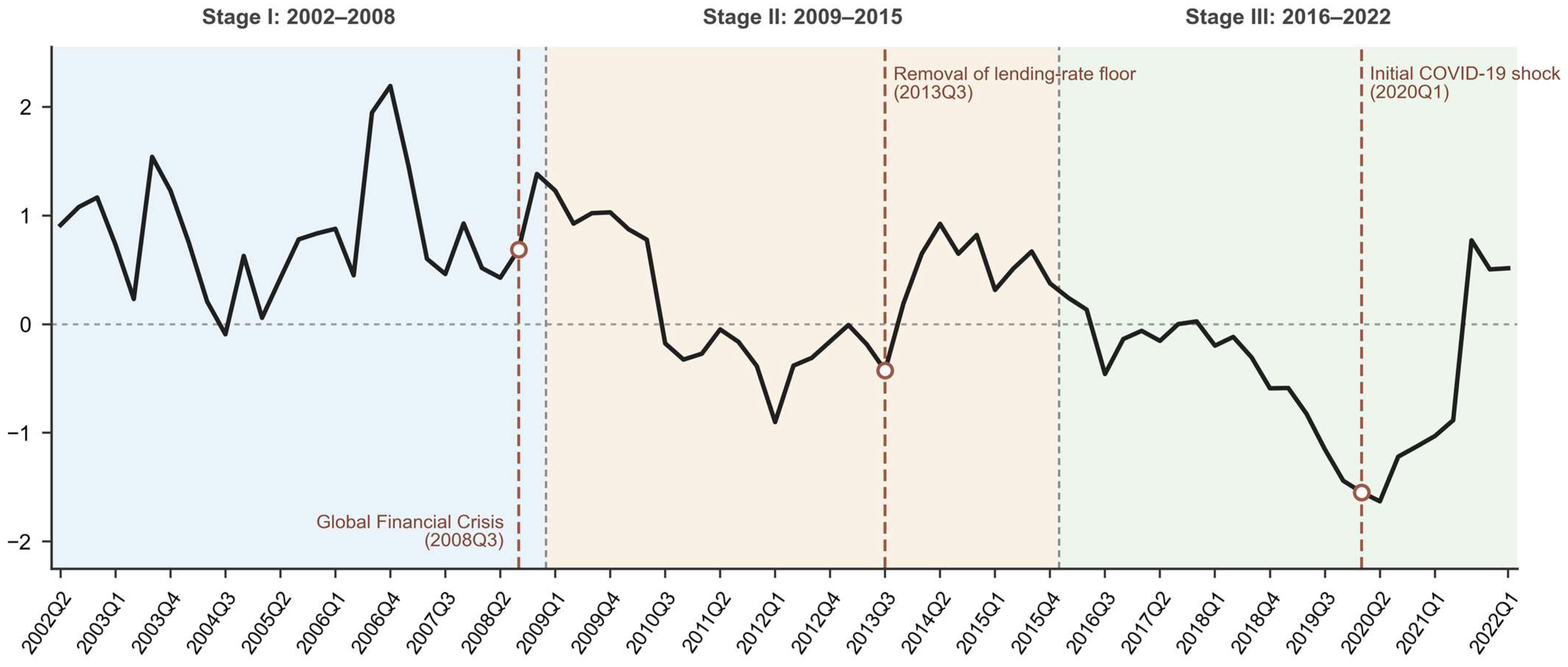
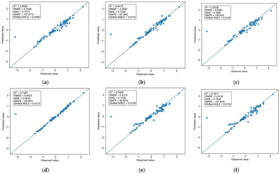
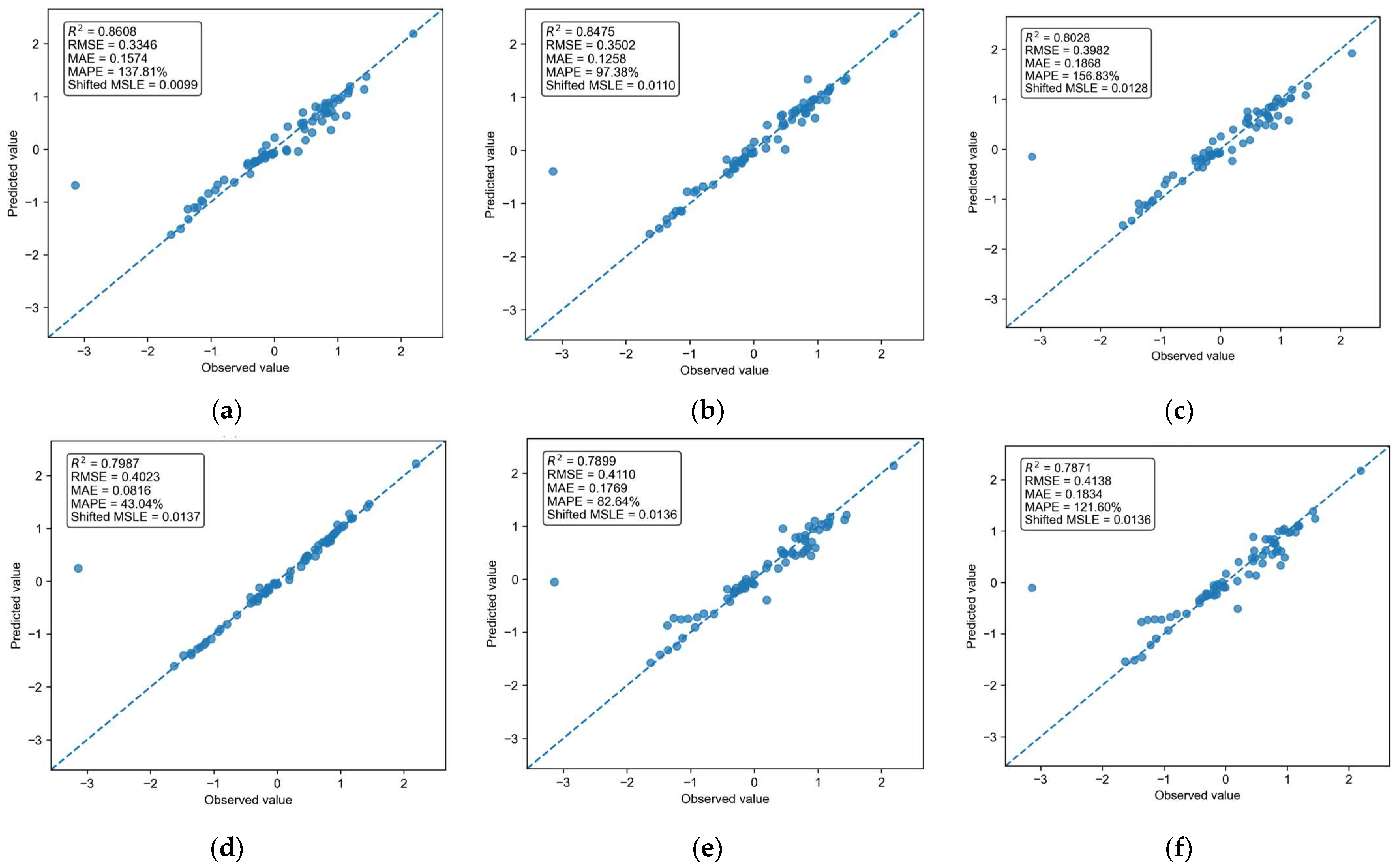
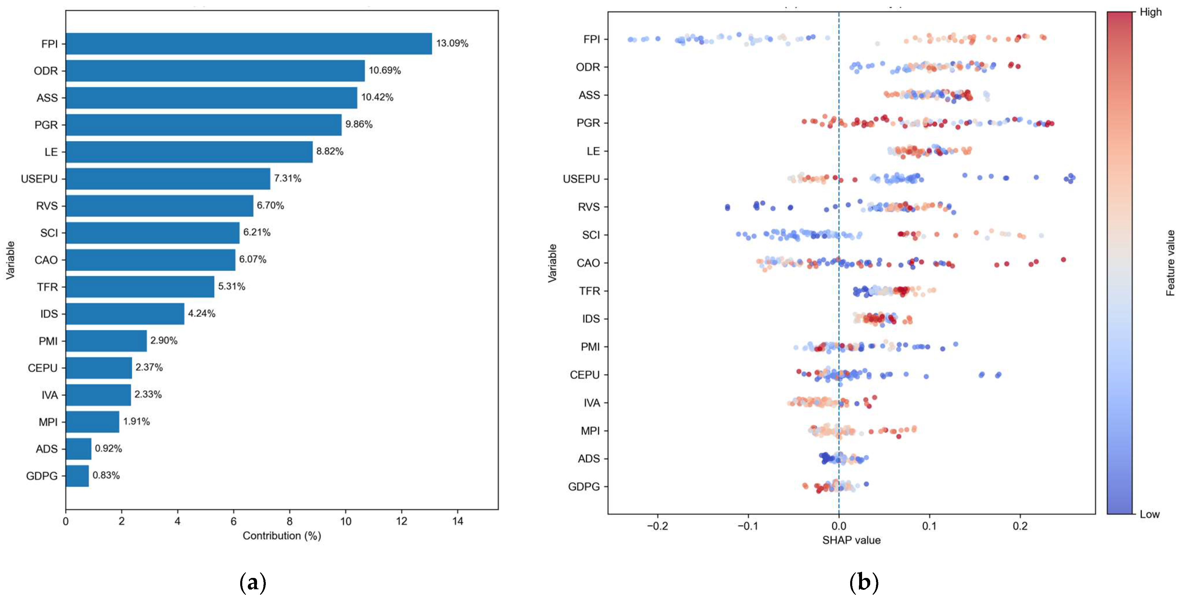
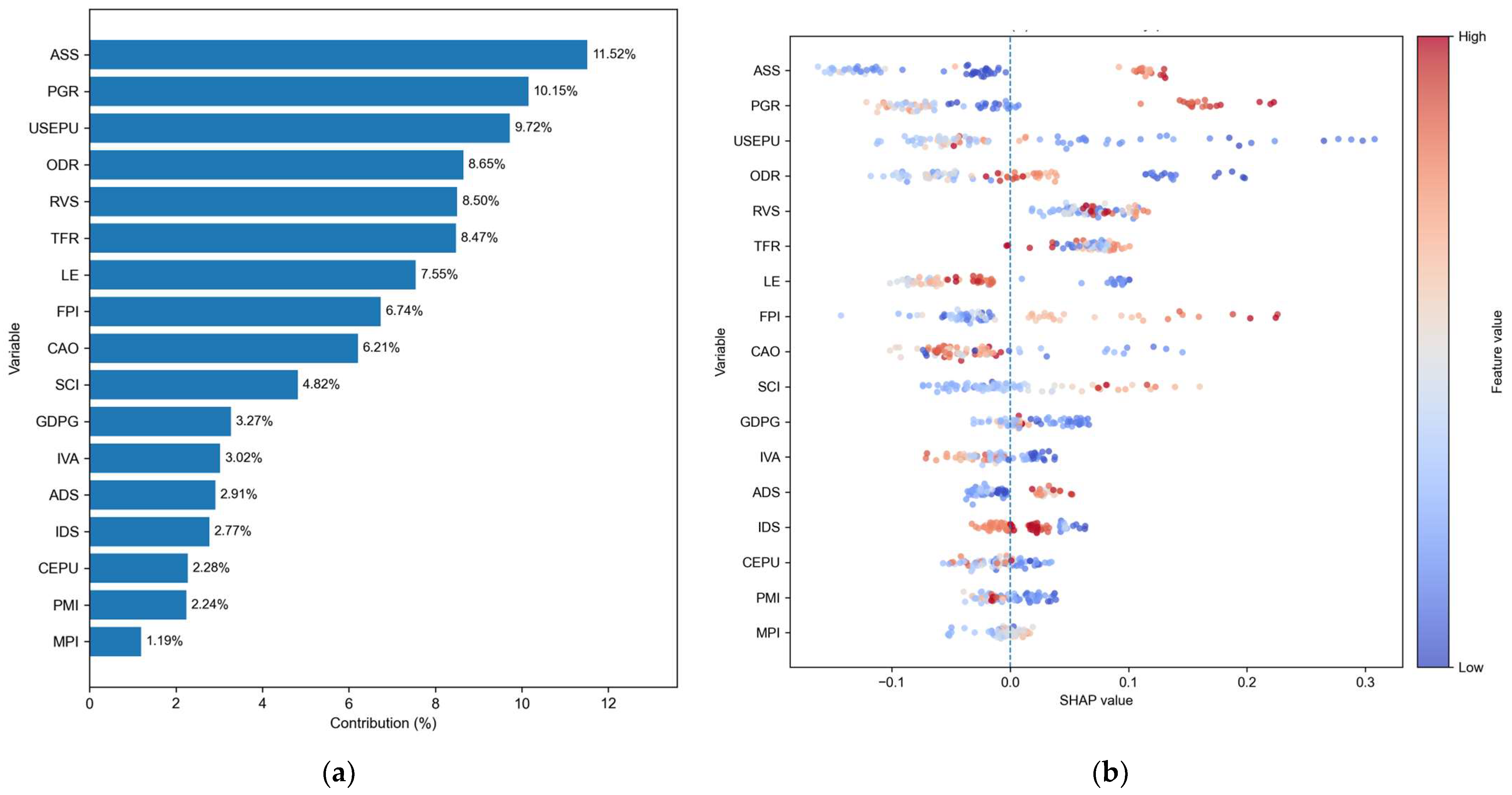
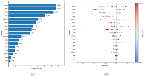
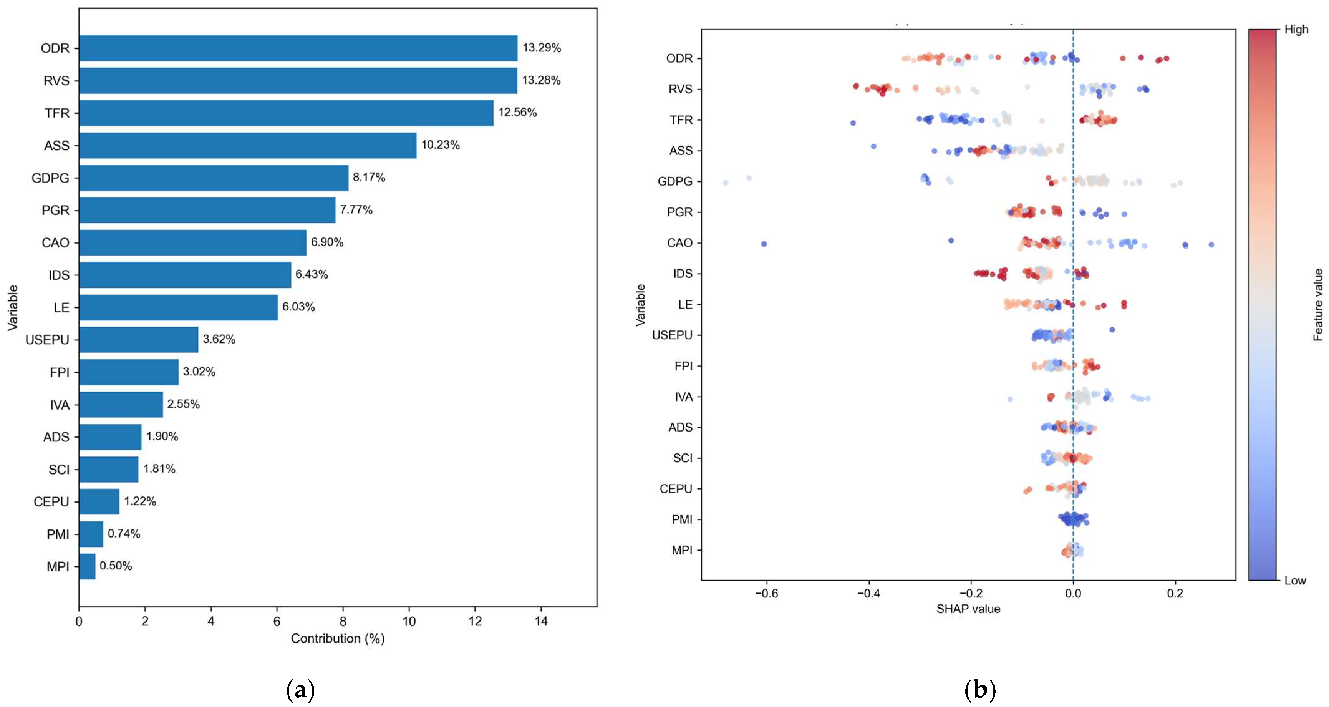
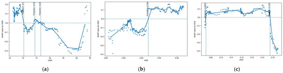
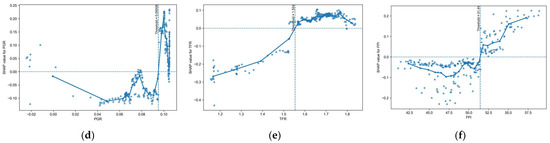
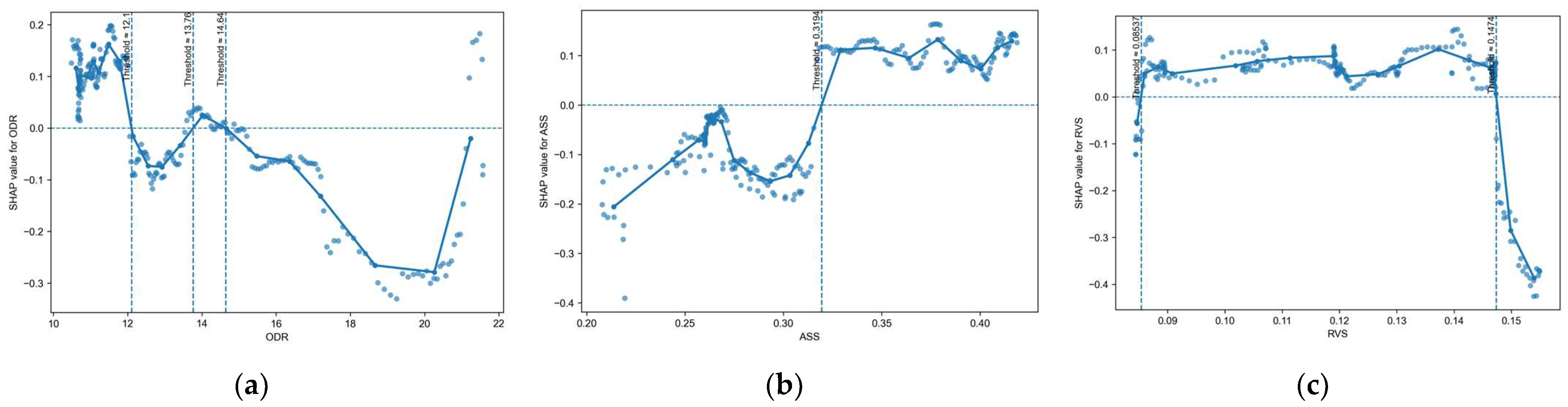
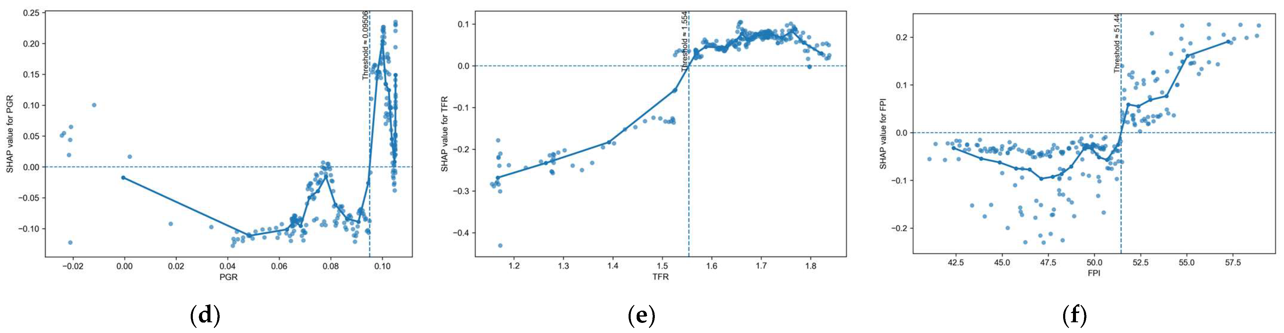

Disclaimer/Publisher’s Note: The statements, opinions and data contained in all publications are solely those of the individual author(s) and contributor(s) and not of MDPI and/or the editor(s). MDPI and/or the editor(s) disclaim responsibility for any injury to people or property resulting from any ideas, methods, instructions or products referred to in the content. |
© 2026 by the authors. Licensee MDPI, Basel, Switzerland. This article is an open access article distributed under the terms and conditions of the Creative Commons Attribution (CC BY) license.