A Risk Minimization Model for Capital Asset Portfolios

Abstract

In 1952, Harry Markowitz established the foundations of Modern Portfolio Theory by introducing a mean–variance framework for constructing investment portfolios that optimize the trade-off between risk and expected return. Expanding upon this classical framework, this paper develops an analytical algorithm to determine optimal asset weights for long-only portfolios that minimize total risk. We derive the necessary and sufficient conditions through rigorous determinant-based identities, providing a closed-form solution for achieving the global minimum variance. The theoretical findings are demonstrated through three numerical examples: the first examines a standard six-asset portfolio using an admissible covariance matrix; the second serves as an algebraic cautionary case by identifying negative variance when the input matrix fails to satisfy the criteria for positive definiteness; and the third example validates the practical application of the proposed identities using empirical market data.

1. Introduction

An investment portfolio is a combination of assets held for investment purposes, including financial, tangible, and intangible assets. In the present study, the focus is on portfolios of capital assets (referred to as investment instruments), although the conclusions are broadly applicable to the general case.

Portfolios improve investment outcomes by combining assets to achieve risk–return profiles unattainable individually. In 1952, Markowitz (1952) formalized diversification by introducing measures of portfolio risk and expected return and defining “efficient portfolios” that minimize risk for a given return or maximize return for a given risk. His framework yields a set of optimal portfolios, from which investors choose according to their preferences. While expected return is a weighted average of asset returns, portfolio risk depends on both individual risks and covariances. The effect of adding an asset often depends more on its correlations with existing assets than on its standalone risk.

The theory of portfolio selection has its origins in the pioneering work by Markowitz (1952, 1959), who introduced the mean–variance framework to optimize the trade-off between expected return and risk and formalized the concept of efficient diversification. This framework laid the foundation for modern portfolio theory and practical investment strategies.

Building on Markowitz’s idea, Tobin (1958) explored investors’ behavior towards risk and liquidity preference, while Sharpe (1963, 1964, 1967) and Lintner (1965) developed models such as CAPM and linear programming approaches for portfolio selection, providing a theoretical bridge between asset pricing and portfolio construction. Subsequent textbooks and comprehensive treatments by Elton and Gruber (1995), Fabozzi (2001), Reilly and Brown (2002), and Bodie et al. (2017) consolidated these theories and extended their practical applications.

Recent research has focused on refining the mean–variance framework and incorporating alternative risk measures. Zhang et al. (2018) reviewed methodological innovations and practical modifications of the Markowitz model, while Rigamonti (2020) highlighted its continued relevance due to interpretability and computational tractability. Extensions using Conditional Value-at-Risk (CVaR) have been proposed to improve downside risk management, as shown by Li and Xu (2013) and Razak et al. (2019). Further studies addressed robustness and empirical validation, including worst-case optimization (Baviera & Bianchi, 2021), real-world stock portfolio applications (Wang, 2022), and comparative risk–return analyses under varying market conditions (Zhou et al., 2025). Collectively, these works demonstrate that the mean–variance framework remains a cornerstone of portfolio theory, while modern adaptations enhance its practical relevance and effectiveness in contemporary financial markets.

However, a persistent challenge in the evolution from Markowitz’s foundations to the equilibrium models by Sharpe and Lintner is the high sensitivity of the efficient frontier to expected return estimates. This study deepens the Markowitz framework by shifting the focus to the specific isolation of total risk minimization, independent of return expectations. Unlike broader generalizations, our model establishes a direct logical link to the global minimum variance (GMV) point, turning portfolio selection into a rigorous mathematical refinement of the problem first envisioned by Markowitz.

Focusing on long-only portfolios of capital assets without short sales, this study achieves the following results:

• Establishes the existence and coordinates of a stationary point for the portfolio risk function;
• Provides a formal proof that the risk function attains its unique global minimum;
• Derives an exact analytical closed-form representation based on determinant identities.

This approach offers two distinct advantages. First, it augments iterative numerical procedures with an exact determinant-based algebraic representation, thereby establishing a direct functional link between the covariance structure and optimal weights. Second, it provides a necessary and sufficient condition for the existence and uniqueness of the global minimum. While contemporary portfolio construction shifts toward data-driven paradigms, such as generative models Cheng and Chen (2025) or complex risk measures like CVaR Senescall and Low (2024), refining these analytical foundations retains their fundamental value. By linking abstract covariance structures to their direct functional impact, this study provides mathematical clarity regarding the algebraic constraints of the GMV problem that often remains obscured in purely numerical or generative methods. Specifically, the determinantal identities provide a transparent analytical view of how the covariance matrix determines the inclusion or exclusion of certain assets. The sign conditions for the principal minors serve as an algebraic verification for the feasibility of long-only weights, thereby establishing a theoretical foundation for understanding when an interior optimum is maintained before any boundary analysis is required. Reframing the contribution within this determinant-based framework ensures that the proposed approach remains consistent with established analytical foundations while providing new qualitative perspectives into the geometry of the feasible set.

The results are illustrated with three numerical examples. In the first example, we consider a classical portfolio with six capital assets. The second example serves as an algebraic cautionary case by identifying negative variance when the input matrix fails to meet the criteria for positive definiteness. The third example validates the practical application of the proposed identities using empirical market data.

2. Preliminaries

Throughout this section, we define the following notations and conventions that are necessary to formulate the main results.

Given a portfolio of n capital assets $C{A}_1,\dots ,C{A}_n$ whose returns are $R_1,\dots ,R_n$ correspondingly and a variance–covariance matrix

$$\mathsf{\Sigma }=\left(\begin{array}{cccc}{\sigma }_1^2& {\sigma }_{12}& \dots & {\sigma }_{1n}\\ {\sigma }_{12}& {\sigma }_2^2& \dots & {\sigma }_{2n}\\ ⋮& ⋮& \ddots & ⋮\\ {\sigma }_{1n}& {\sigma }_{2n}& \dots & {\sigma }_n^2\end{array}\right).$$

The following inequalities

$$-{\sigma }_i{\sigma }_j\le {\sigma }_{ij}\le {\sigma }_i{\sigma }_j,\mathrm{where}1\le i\le j\le n$$

(1)

hold. The ultimate values of ${\sigma }_{ij}$ correspond to perfectly correlated (negatively or positively) returns $R_i$ and $R_j$. Further, we also used the notation ${\sigma }_{ii}$ instead of ${\sigma }_i^2$, $i=1,\dots ,n=\overline{1,n}$.

According to $\left|B\right|$, we denote the determinant of a quadratic matrix B; according to $B^T$, we denote the transpose of the matrix B. The equality $\left|B^T\right|=\left|B\right|$ holds.

For a quadratic matrix B of order n, the leading principal minors $M_i^B$ (for $i=\overline{1,n}$) are the determinants of the upper-left $(i\times i)$ submatrices:

$$M_1^B=b_{11},M_2^B=\left|\begin{array}{cc}{b}_{11}& b_{12}\\ b_{21}& b_{22}\end{array}\right|,\dots ,M_n^B=\left|B\right|.$$

Theorem 1 

(Fikhtengol’ts (1956, 1957, 1958)). (Sylvester’s Criterion for Positive Definiteness): Let B be a real symmetric matrix of order n. The matrix B is positive definite if and only if all its leading principal minors are strictly positive, i.e., $M_1^B>0,\dots ,M_n^B>0$.

According to Sylvester’s Criterion, a symmetric matrix $\mathsf{\Sigma }$ is positive semi-definite if and only if all its principal minors (not just the leading ones) are non-negative.

The corresponding asset shares in the portfolio are denote by $x_i$, $i=\overline{1,n}$. They satisfy the conditions

$$\sum _{i=1}^n{x}_i=1$$

(2)

and

$$x_i\ge 0\mathrm{for}i=\overline{1,n},$$

(3)

which define the $(n-1)$-dimensional manifold $S_{n-1}$. The last inequalities correspond to the absence of short sales in portfolio assets.

According to the portfolio theory of Markowitz (1952), the portfolio return $R_p$ is given by

$$R_p=\sum _{i=1}^n{R}_i{x}_i$$

(4)

and the portfolio variance ${\sigma }_p^2$ is a quantitative measure of the portfolio risk and is given by

$${\sigma }_p^2=x^T\mathsf{\Sigma }x,$$

(5)

where $x^T=(x_1,\dots ,x_n)$.

Representation (5) is valid only under the assumption that the underlying quadratic form is positive definite. For $n=2$, the matrix $\mathsf{\Sigma }$ satisfies Sylvester’s Criterion (Theorem 1), except in the degenerated cases ${\sigma }_{12}=\pm {\sigma }_1{\sigma }_2$ of perfect correlation between the asset returns. For $n\ge 3$, however, Sylvester’s Criterion may fail to be satisfied if the matrix is not properly constructed, as illustrated in an example below. To ensure that the model remains within the boundaries of standard portfolio theory and that all results are economically interpretable, we shall assume that the matrix $\mathsf{\Sigma }$ is symmetric and positive semi-definite, ensuring that ${\sigma }_p^2\left(x\right)\ge 0$ for all asset weights. While positive semi-definiteness is sufficient to maintain the probabilistic integrity of the variance, the stronger requirement of positive definiteness ensures that the Hessian of the objective function is positive definite, thereby providing the strict convexity necessary for the existence of a unique stationary point and an optimal weight vector.

The first problem involves determining the conditions under which a minimum-risk $min{\sigma }_p^2\left(x\right)$ portfolio exists on the manifold $S_{n-1}$ and the corresponding asset weights. To establish the existence of a critical point of the function ${\sigma }_p^2\left(x\right)$ over $S_{n-1}$ and to derive its coordinates, the variables are reduced using Equality (2). The existence of a minimum at this critical point is demonstrated via Sylvester’s Criterion. The coordinates of the critical point, the minimum portfolio risk, and the corresponding portfolio return are then expressed in a compact and explicit form in terms of the determinant of the portfolio matrix and its extensions. All computations in the examples considered for $n=\overline{2,6}$ are performed using Wolfram Mathematica 14.

We introduce the notations

$${\tilde{x}}^T=(x_1,\dots ,x_{n-1}),b^T=(b_1,\dots ,b_{n-1}),\mathrm{where}{b}_i={\sigma }_n^2-{\sigma }_{in}.$$

Let $A=\left(a_{ij}\right)$, $a_{ij}=b_i+c_{ij}$, $c_{ij}={\sigma }_{ij}-{\sigma }_{jn}$, $c_j^T=(c_{1j},\dots ,c_{(n-1)j})$, $i,j=\overline{1,n-1}$. We also denote ${\displaystyle r=\underset{i=\overline{1,n}}{min}\left\{R_i\right\}}$, ${\displaystyle R=\underset{i=\overline{1,n}}{max}\left\{R_i\right\}}$ and

$${\mathsf{\Sigma }}_i=\left(\begin{array}{cccccccc}{\sigma }_1^2& {\sigma }_{12}& \dots & {\sigma }_{1i-1}& 1& {\sigma }_{1i+1}& \dots & {\sigma }_{1n}\\ {\sigma }_{12}& {\sigma }_2^2& \dots & {\sigma }_{2i-1}& 1& {\sigma }_{2i+1}& \dots & {\sigma }_{2n}\\ ⋮& ⋮& \ddots & ⋮& ⋮& ⋮& \dots & \\ {\sigma }_{1n}& {\sigma }_{2n}& \dots & {\sigma }_{i-1n}& 1& {\sigma }_{i+1n}& \dots & {\sigma }_n^2\end{array}\right),$$

$$\left(\begin{array}{cc}\mathsf{\Sigma }& 1\\ 1& 0\end{array}\right)=\left(\begin{array}{ccccc}{\sigma }_1^2& {\sigma }_{12}& \dots & {\sigma }_{1n}& 1\\ {\sigma }_{12}& {\sigma }_2^2& \dots & {\sigma }_{2n}& 1\\ ⋮& ⋮& \ddots & ⋮& \\ {\sigma }_{1n}& {\sigma }_{2n}& \dots & {\sigma }_n^2& 1\\ 1& 1& \dots & 1& 0\end{array}\right),\left(\begin{array}{cc}\mathsf{\Sigma }& 1\\ R& 0\end{array}\right)=\left(\begin{array}{ccccc}{\sigma }_1^2& {\sigma }_{12}& \dots & {\sigma }_{1n}& 1\\ {\sigma }_{12}& {\sigma }_2^2& \dots & {\sigma }_{2n}& 1\\ ⋮& ⋮& \ddots & ⋮& \\ {\sigma }_{1n}& {\sigma }_{2n}& \dots & {\sigma }_n^2& 1\\ R_1& R_2& \dots & R_n& 0\end{array}\right).$$

3. Main Results

The task to be solved in the present study consists of determining the conditions for the existence of a portfolio with minimal risk $\left(\min {\sigma }_p^2\right)$ and the corresponding asset shares on the manifold $S_{n-1}$.

First, we shall prove two auxiliary lemmas.

Lemma 1. 

For the matrix Σ, the equality

$$-\left|\begin{array}{cc}\mathsf{\Sigma }& 1\\ 1& 0\end{array}\right|=\sum _{i=1}^n\left|{\mathsf{\Sigma }}_i\right|$$

(6)

holds.

Proof. 

By expanding the determinant $-\left|\begin{array}{cc}\mathsf{\Sigma }& 1\\ 1& 0\end{array}\right|$ with respect to the elements of its last row, we obtain

$$\begin{array}{c}-\left|\begin{array}{ccccc}{\sigma }_1^2& {\sigma }_{12}& \dots & {\sigma }_{1n}& 1\\ {\sigma }_{12}& {\sigma }_2^2& \dots & {\sigma }_{2n}& 1\\ \dots & \dots & \dots & \dots & \dots \\ {\sigma }_{1n}& {\sigma }_{2n}& \dots & {\sigma }_n^2& 1\\ 1& 1& \dots & 1& 0\end{array}\right|={(-1)}^{n+3}\left|\begin{array}{cccc}{\sigma }_{12}& \dots & {\sigma }_{1n}& 1\\ {\sigma }_2^2& \dots & {\sigma }_{2n}& 1\\ \dots & \dots & \dots & \dots \\ {\sigma }_{2n}& \dots & {\sigma }_n^2& 1\end{array}\right|\hfill \\ +{(-1)}^{n+4}\left|\begin{array}{cccc}{\sigma }_1^2& \dots & {\sigma }_{1n}& 1\\ {\sigma }_{12}& \dots & {\sigma }_{2n}& 1\\ \dots & \dots & \dots & \dots \\ {\sigma }_{1n}& \dots & {\sigma }_n^2& 1\end{array}\right|+\dots +{(-1)}^{2n+2}\left|\begin{array}{cccc}{\sigma }_1^2& \dots & {\sigma }_{1n-1}& 1\\ {\sigma }_{12}& \dots & {\sigma }_{2n-1}& 1\\ \dots & \dots & \dots & \dots \\ {\sigma }_{1n}& \dots & {\sigma }_{n-1n}& 1\end{array}\right|\hfill \\ ={(-1)}^4{(-1)}^{n-1}\left|\begin{array}{cccc}{\sigma }_{12}& \dots & {\sigma }_{1n}& 1\\ {\sigma }_2^2& \dots & {\sigma }_{2n}& 1\\ \dots & \dots & \dots & \dots \\ {\sigma }_{2n}& \dots & {\sigma }_n^2& 1\end{array}\right|+{(-1)}^6{(-1)}^{n-2}\left|\begin{array}{cccc}{\sigma }_1^2& \dots & {\sigma }_{1n}& 1\\ {\sigma }_{12}& \dots & {\sigma }_{2n}& 1\\ \dots & \dots & \dots & \dots \\ {\sigma }_{1n}& \dots & {\sigma }_n^2& 1\end{array}\right|+\dots \hfill \\ +{(-1)}^{2n+2}\left|\begin{array}{cccc}{\sigma }_1^2& \dots & {\sigma }_{1n-1}& 1\\ {\sigma }_{12}& \dots & {\sigma }_{2n-1}& 1\\ \dots & \dots & \dots & \dots \\ {\sigma }_{1n}& \dots & {\sigma }_{n-1n}& 1\end{array}\right|\hfill \\ =\left|\begin{array}{cccc}1& {\sigma }_{12}& \dots & {\sigma }_{1n}\\ 1& {\sigma }_2^2& \dots & {\sigma }_{2n}\\ \dots & \dots & \dots & \dots \\ 1& {\sigma }_{2n}& \dots & {\sigma }_n^2\end{array}\right|+\left|\begin{array}{cccc}{\sigma }_1^2& 1& \dots & {\sigma }_{1n}\\ {\sigma }_{12}& 1& \dots & {\sigma }_{2n}\\ \dots & \dots & \dots & \dots \\ {\sigma }_{1n}& 1& \dots & {\sigma }_n^2\end{array}\right|+\dots +\left|\begin{array}{cccc}{\sigma }_1^2& {\sigma }_{12}& \dots & 1\\ {\sigma }_{12}& {\sigma }_2^2& \dots & 1\\ \dots & \dots & \dots & \dots \\ {\sigma }_{1n}& {\sigma }_{2n}& \dots & 1\end{array}\right|,\hfill \end{array}$$

which proves Equality (6). □

Lemma 2. 

For every $i=\overline{1,n-1}$, the following equalities are valid:

$$\left|\begin{array}{cccccc}{\sigma }_1^2& {\sigma }_{12}& \dots & {\sigma }_{1i}& {\sigma }_{1n}& 1\\ {\sigma }_{12}& {\sigma }_2^2& \dots & {\sigma }_{2i}& {\sigma }_{2n}& 1\\ \dots & \dots & \dots & \dots & \dots & \dots \\ {\sigma }_{1i}& {\sigma }_{2i}& \dots & {\sigma }_i^2& {\sigma }_{in}& 1\\ {\sigma }_{1n}& {\sigma }_{2n}& \dots & {\sigma }_{in}& {\sigma }_n^2& 1\\ 1& 1& \dots & 1& 1& 0\end{array}\right|=-\left|\begin{array}{cccc}{a}_{11}& a_{12}& \dots & a_{1i}\\ a_{21}& a_{22}& \dots & a_{2i}\\ \dots & \dots & \dots & \dots \\ a_{i1}& a_{i2}& \dots & a_{ii}\end{array}\right|.$$

Proof. 

The matrix $A=\left(a_{ij}\right)$ is symmetric since

$$a_{ij}=b_i+c_{ij}={\sigma }_n^2-{\sigma }_{in}+{\sigma }_{ij}-{\sigma }_{jn}={\sigma }_n^2-{\sigma }_{jn}+{\sigma }_{ij}-{\sigma }_{in}=b_j+c_{ji}=a_{ji}$$

for $i,j=\overline{1,n-1}$ due to ${\sigma }_{ij}={\sigma }_{ji}$ for $i,j=\overline{1,n}$. By applying suitable transformations while keeping i ($1\le i\le n-1$) fixed, we obtain

$$\begin{array}{c}\left|\begin{array}{cccccc}{\sigma }_1^2& {\sigma }_{12}& \dots & {\sigma }_{1i}& {\sigma }_{1n}& 1\\ {\sigma }_{12}& {\sigma }_2^2& \dots & {\sigma }_{2i}& {\sigma }_{2n}& 1\\ \dots & \dots & \dots & \dots & \dots & \dots \\ {\sigma }_{1i}& {\sigma }_{2i}& \dots & {\sigma }_i^2& {\sigma }_{in}& 1\\ {\sigma }_{1n}& {\sigma }_{2n}& \dots & {\sigma }_{in}& {\sigma }_n^2& 1\\ 1& 1& \dots & 1& 1& 0\end{array}\right|=\left|\begin{array}{cccccc}{c}_{11}& c_{12}& \dots & c_{1i}& -b_1& 0\\ c_{21}& c_{22}& \dots & c_{2i}& -b_2& 0\\ \dots & \dots & \dots & \dots & \dots & \dots \\ c_{i1}& c_{i2}& \dots & c_{ii}& -b_i& 0\\ {\sigma }_{1n}& {\sigma }_{2n}& \dots & {\sigma }_{in}& {\sigma }_n^2& 1\\ 1& 1& \dots & 1& 1& 0\end{array}\right|\hfill \\ =-\left|\begin{array}{ccccc}{c}_{11}& c_{12}& \dots & c_{1i}& -b_1\\ c_{21}& c_{22}& \dots & c_{2i}& -b_2\\ \dots & \dots & \dots & \dots & \dots \\ c_{i1}& c_{i2}& \dots & c_{ii}& -b_i\\ 1& 1& \dots & 1& 1\end{array}\right|=-\left|\begin{array}{ccccc}{a}_{11}& a_{12}& \dots & a_{1i}& -b_1\\ a_{12}& a_{22}& \dots & a_{2i}& -b_2\\ \dots & \dots & \dots & \dots & \dots \\ a_{1i}& a_{2i}& \dots & a_{ii}& -b_i\\ 0& 0& \dots & 0& 1\end{array}\right|\hfill \\ =-\left|\begin{array}{cccc}{a}_{11}& a_{12}& \dots & a_{1i}\\ a_{12}& a_{22}& \dots & a_i\\ \dots & \dots & \dots & \dots \\ a_{1i}& a_{2i}& \dots & a_{ii}\end{array}\right|=-M_i^A,\hfill \end{array}$$

where $M_i^A$ denotes the leading principal minor of order i of the matrix A. For $i=n-1$, we obtain

$$\left|\begin{array}{cc}\mathsf{\Sigma }& 1\\ 1& 0\end{array}\right|=-M_{n-1}^A=-\left|A\right|,$$

(7)

which completes the proof. □

Now we are ready to state the first main result.

Theorem 2. 

Let the matrix Σ fulfill the following inequalities:

$$|{\mathsf{\Sigma }}_i|\ge 0\mathrm{with}\sum _{i=1}^n\left|{\mathsf{\Sigma }}_i\right|>0,i=\overline{1,n}.$$

(8)

Then, ${\sigma }_p^2\left(x\right)$ has a unique conditional critical (stationary) point on $S_{n-1}$.

Proof. 

We use Equality (2) to express $x_n$ in terms of the remaining $n-1$ variables and substitute it into Equality (5); we then obtain

$${\sigma }_p^2\left(\tilde{x}\right)={\tilde{x}}^{T}A\tilde{x}-2b^T\tilde{x}+{\sigma }_n^2.$$

(9)

From (8), (6) and (7), it follows that $\left|A\right|\ne 0$. Then, the equation

$${\left({\sigma }_p^2\left(\tilde{x}\right)\right)}^{\prime }=2(A\tilde{x}-b)=\mathbf{0},\mathrm{where}\mathbf{0}=(\underset{n-1}{\underbrace{0,\dots ,0}})$$

(10)

has a unique solution

$${\tilde{x}}^{\ast }=A^{-1}b,$$

(11)

which is the critical point of the quadratic function ${\sigma }_p^2\left(\tilde{x}\right)$. The coordinates of the solution ${\tilde{x}}^{\ast }$ for $i=1,\dots ,n-1$ are

$$x_i^{\ast }={\displaystyle \frac{|A_i|}{\left|A\right|}},$$

(12)

where

$$A_i=\left(\begin{array}{cccccccc}{a}_{11}& a_{12}& \dots & a_{1i-1}& b_1& a_{1i+1}& \dots & a_{1n-1}\\ a_{12}& a_{22}& \dots & a_{2i-1}& b_2& a_{2i+1}& \dots & a_{1n-1}\\ \dots & \dots & \dots & \dots & \dots & \dots & \dots & \dots \\ a_{1n-1}& a_{2n-1}& \dots & a_{i-1n-1}& b_{n-1}& a_{i+1n-1}& \dots & a_{n-1n-1}\end{array}\right).$$

From

$$\begin{array}{cc}|A_i|& =|b+c_1\dots b+c_{i-1}bb+c_{i+1}\dots b+c_{n-1}|\hfill \\ & =|c_1\dots c_{i-1}b{c}_{i+1}\dots c_{n-1}|.\hfill \end{array}$$

and

$$\begin{array}{cc}|{\mathsf{\Sigma }}_i|& =\left|\begin{array}{cccccccc}{\sigma }_1^2& {\sigma }_{12}& \dots & {\sigma }_{1i-1}& 1& {\sigma }_{1i+1}& \dots & {\sigma }_{1n}\\ {\sigma }_{12}& {\sigma }_2^2& \dots & {\sigma }_{2i-1}& 1& {\sigma }_{2i+1}& \dots & {\sigma }_{2n}\\ ⋮& ⋮& \ddots & ⋮& ⋮& ⋮& \dots & \\ {\sigma }_{1n}& {\sigma }_{2n}& \dots & {\sigma }_{i-1n}& 1& {\sigma }_{i+1n}& \dots & {\sigma }_n^2\end{array}\right|\hfill \\ & =\left|\begin{array}{ccccccccc}{c}_1& c_2& \dots & c_{i-1}& 0& c_{i+1}& \dots & c_{n-1}& -b\\ {\sigma }_{1n}& {\sigma }_{2n}& \dots & {\sigma }_{i-1n}& 1& {\sigma }_{i+1n}& \dots & {\sigma }_{n-1n}& {\sigma }_n^2\end{array}\right|\hfill \\ & ={(-1)}^{n+i}|c_1\dots c_{i-1}{c}_{i+1}\dots c_{n-1}-b|\hfill \\ & ={(-1)}^{n+i+1}|c_1\dots c_{i-1}{c}_{i+1}\dots c_{n-1}b|\hfill \\ & =|c_1\dots c_{i-1}b{c}_{i+1}\dots c_{n-1}|=|A_i|\hfill \end{array}$$

we deduce that

$$\left|A_i\right|=\left|{\mathsf{\Sigma }}_i\right|,i=\overline{1,n-1}.$$

(13)

By combining (13) with (7), from (12) we obtain

$$x_i^{\ast }={\displaystyle \frac{|{\mathsf{\Sigma }}_i|}{-\left|\begin{array}{cc}\mathsf{\Sigma }& 1\\ 1& 0\end{array}\right|}}\mathrm{for}i=\overline{1,n-1}.$$

(14)

From (6) and (8), we conclude that the numbers $-\left|\begin{array}{cc}\mathsf{\Sigma }& 1\\ 1& 0\end{array}\right|$ and $\left|{\mathsf{\Sigma }}_i\right|,i=\overline{1,n}$ have the same sign. This implies that $0\le x_i^{\ast }\le 1,i=\overline{1,n-1}$. On the other hand, we have

$$x_n^{\ast }=1-{\displaystyle \sum _{i=1}^{n-1}}{x}_i^{\ast }=1-{\displaystyle \frac{{\displaystyle \sum _{i=1}^{n-1}}\left|{\mathsf{\Sigma }}_i\right|}{-\left|\begin{array}{cc}\mathsf{\Sigma }& 1\\ 1& 0\end{array}\right|}}={\displaystyle \frac{\left|{\mathsf{\Sigma }}_n\right|}{-\left|\begin{array}{cc}\mathsf{\Sigma }& 1\\ 1& 0\end{array}\right|}}\in \left[0,1\right].$$

Therefore, the point $x^{\ast }$ with coordinates

$$x_i^{\ast }={\displaystyle \frac{\left|{\mathsf{\Sigma }}_i\right|}{-\left|\begin{array}{cc}\mathsf{\Sigma }& 1\\ 1& 0\end{array}\right|}},i=\overline{1,n}$$

(15)

is a critical point for ${\sigma }_p^2\left(x\right)$ under condition (2) and $x^{\ast }\in S_{n-1}$. This completes the proof of the theorem. □

Remark 1. 

Theorem 2 also holds under the condition ${\displaystyle |{\mathsf{\Sigma }}_i|\le 0\mathrm{with}\sum _{i=1}^n\left|{\mathsf{\Sigma }}_i\right|<0,i=\overline{1,n}.}$ However, it is important to note that these inequalities ensure non-negative asset weights (i.e., the existence of a conditional stationary point for the quadratic function ${\sigma }_p^2\left(x\right)$), but they imply $M_{n-1}^A=\left|A\right|<0$. According to Sylvester’s Criterion, this indicates that a minimum is not attained at this critical point.

With the following theorem, we provide a necessary and sufficient condition for a local minimum at the previously established critical point.

Theorem 3. 

Assume that Theorem 2 holds. The function ${\sigma }_p^2\left(x\right)$ has a conditional minimum at the point $x^{\ast }$ if and only if the inequalities

$$\left|\begin{array}{cccccc}{\sigma }_1^2& {\sigma }_{12}& \dots & {\sigma }_{1i}& {\sigma }_{1n}& 1\\ {\sigma }_{12}& {\sigma }_2^2& \dots & {\sigma }_{2i}& {\sigma }_{2n}& 1\\ \dots & \dots & \dots & \dots & \dots & \dots \\ {\sigma }_{1i}& {\sigma }_{2i}& \dots & {\sigma }_i^2& {\sigma }_{in}& 1\\ {\sigma }_{1n}& {\sigma }_{2n}& \dots & {\sigma }_{in}& {\sigma }_n^2& 1\\ 1& 1& \dots & 1& 1& 0\end{array}\right|<0,i=\overline{1,n-1}.$$

(16)

are satisfied.

Proof. 

Necessity (⟹): Assume that ${\sigma }_p^2\left(x\right)$ has a conditional minimum at $x^{\ast }$. This coincides with the minimum of ${\sigma }_p^2\left(\tilde{x}\right)$ at ${\tilde{x}}^{\ast }$ by virtue of condition (2). By substituting ${\tilde{x}}^{\ast }$ from (11) into (9), we get

$${\sigma }_p^2\left({\tilde{x}}^{\ast }\right)={\sigma }_n^2-b^T{A}^{-1}b.$$

(17)

We write Equality (9) in its equivalent form

$${\sigma }_p^2\left(\tilde{x}\right)={(\tilde{x}-A^{-1}b)}^{T}A(\tilde{x}-A^{-1}b)-b^T{A}^{-1}b+{\sigma }_n^2.$$

(18)

From (17) and (18), it follows that

$${\sigma }_p^2\left(\tilde{x}\right)-{\sigma }_p^2\left({\tilde{x}}^{\ast }\right)={(\tilde{x}-{\tilde{x}}^{\ast })}^{T}A(\tilde{x}-{\tilde{x}}^{\ast }).$$

(19)

The inequality ${\sigma }_p^2\left(\tilde{x}\right)-{\sigma }_p^2\left({\tilde{x}}^{\ast }\right)>0$ holds for every $\tilde{x}\in S_{n-1},\tilde{x}\ne {\tilde{x}}^{\ast }$. This makes the quadratic form on the right-hand side of (19) and the matrix A positive definite. By Sylvester’s Criterion, it follows that all leading principal minors of A are positive; i.e., Inequalities (16) are satisfied for $i=1,\dots ,n-1$.

Sufficiency (⟸): From Inequalities (16) and the remark, it follows that all principal minors of A are positive. Then, according to Sylvester’s Criterion (Theorem 1), the matrix A is positive definite. This is a necessary and sufficient condition for the positive definiteness of the quadratic form on the right-hand side of Equality (19), i.e., ${\sigma }_p^2\left(\tilde{x}\right)-{\sigma }_p^2\left({\tilde{x}}^{\ast }\right)>0$, for every $\tilde{x}\in S_{n-1}$, $\tilde{x}\ne {\tilde{x}}^{\ast }$. Therefore, the function ${\sigma }_p^2\left(\tilde{x}\right)$ has a local minimum at the point ${\tilde{x}}^{\ast }$, which coincides with the constrained minimum of the function ${\sigma }_p^2\left(x\right)$ at the point $x^{\ast }$ under condition (2), i.e.,

$$min{\sigma }_p^2\left(\tilde{x}\right)={\sigma }_p^2\left({\tilde{x}}^{\ast }\right)=min{\sigma }_p^2\left(x\right){|}_{\left(2\right)}={\sigma }_p^2\left(x^{\ast }\right).$$

(20)

This completes the proof of the theorem. □

Remark 2. 

It is important to note that Theorem 3 characterizes the analytical structure of the interior optimum within the feasible set. In the context of constrained optimization, determinant-sign condition (8) serves as an algebraic filter to determine whether the optimal solution satisfies the non-negativity requirements for $x_i\ge 0$. If this condition is met, the minimum is guaranteed to lie on the feasible set, meaning that all assets with positive weights are included. If determinantal condition (8) is violated, it indicates that the unconstrained minimum lies outside the feasible set, implying that the constrained optimum is located on the boundary. In such cases, assets with non-positive weights are excluded from the “active set” (the assets with positive weights). In this context, the proposed determinantal framework may serve as analytical prerequisite that facilitates the identification of the optimal subset of assets.

In the next theorem, we establish formulas for calculating the risk at the point of local minimum and the corresponding average return.

Theorem 4. 

Assume that Theorem 2 holds. Then

$$min{\sigma }_p^2\left(x\right){|}_{\left(2\right)}={\sigma }_p^2\left(x^{\ast }\right)={\displaystyle \frac{\left|\mathsf{\Sigma }\right|}{-\left|\begin{array}{cc}\mathsf{\Sigma }& 1\\ 1& 0\end{array}\right|}}$$

(21)

holds.

Proof. 

Using Equalities (20), (11), (14) and (6), we obtain

$$\begin{array}{ccc}& min{\sigma }_p^2\left(x\right){|}_{\left(2\right)}& ={\sigma }_n^2-b^T{\tilde{x}}^{\ast }={\sigma }_n^2-{\left({\tilde{x}}^{\ast }\right)}^{T}b\hfill \\ & & ={\sigma }_n^2-{\displaystyle \frac{1}{{\sum }_{i=1}^n{\mathsf{\Sigma }}_i}}\left(|{\mathsf{\Sigma }}_1\left|\right|{\mathsf{\Sigma }}_2|\dots |{\mathsf{\Sigma }}_{n-1}|\right)\left(\begin{array}{c}{\sigma }_n^2-{\sigma }_{1n}\\ {\sigma }_n^2-{\sigma }_{2n}\\ ⋮\\ {\sigma }_n^2-{\sigma }_{n-1n}\end{array}\right)\hfill \\ & & ={\sigma }_n^2-{\displaystyle \frac{{\displaystyle {\sigma }_n^2\sum _{i=1}^{n-1}|{\mathsf{\Sigma }}_i|-\sum _{i=1}^{n-1}{\sigma }_{in}\left|{\mathsf{\Sigma }}_i\right|}}{{\displaystyle \sum _{i=1}^n\left|{\mathsf{\Sigma }}_i\right|}}}={\displaystyle \frac{{\displaystyle \sum _{i=1}^n{\sigma }_{in}\left|{\mathsf{\Sigma }}_i\right|}}{-\left|\begin{array}{cc}\mathsf{\Sigma }& 1\\ 1& 0\end{array}\right|}}.\hfill \end{array}$$

On the other hand, we have

$$\begin{array}{c}{\displaystyle \sum _{i=1}^n{\sigma }_{in}\left|{\mathsf{\Sigma }}_i\right|={\sigma }_{1n}\left|\begin{array}{ccccc}1& {\sigma }_{12}& {\sigma }_{13}& \dots & {\sigma }_{1n}\\ 1& {\sigma }_2^2& {\sigma }_{23}& \dots & {\sigma }_{2n}\\ 1& {\sigma }_{23}& {\sigma }_3^2& \dots & {\sigma }_{3n}\\ ⋮& ⋮& ⋮& ⋮& ⋮\\ 1& {\sigma }_{2n}& {\sigma }_{3n}& \dots & {\sigma }_n^2\end{array}\right|+{\sigma }_{2n}\left|\begin{array}{ccccc}{\sigma }_1^2& 1& {\sigma }_{13}& \dots & {\sigma }_{1n}\\ {\sigma }_{12}& 1& {\sigma }_{23}& \dots & {\sigma }_{2n}\\ {\sigma }_{13}& 1& {\sigma }_3^2& \dots & {\sigma }_{3n}\\ ⋮& ⋮& ⋮& ⋮& ⋮\\ {\sigma }_{1n}& 1& {\sigma }_{3n}& \dots & {\sigma }_n^2\end{array}\right|+\dots }\hfill \\ +{\sigma }_n^2\left|\begin{array}{ccccc}{\sigma }_1^2& {\sigma }_{12}& {\sigma }_{13}& \dots & 1\\ {\sigma }_{12}& {\sigma }_2^2& {\sigma }_{23}& \dots & 1\\ {\sigma }_{13}& {\sigma }_{23}& {\sigma }_3^2& \dots & 1\\ ⋮& ⋮& ⋮& ⋮& ⋮\\ {\sigma }_{1n}& {\sigma }_{2n}& {\sigma }_{3n}& \dots & 1\end{array}\right|={\sigma }_{1n}\left|\begin{array}{cccccc}0& c_2& c_3& \dots & c_{n-1}& -b\\ 1& {\sigma }_{2n}& {\sigma }_{3n}& \dots & {\sigma }_{n-1n}& {\sigma }_n^2\end{array}\right|\hfill \\ +{\sigma }_{2n}\left|\begin{array}{cccccc}{c}_1& 0& c_3& \dots & c_{n-1}& -b\\ {\sigma }_{1n}& 1& {\sigma }_{3n}& \dots & {\sigma }_{n-1n}& {\sigma }_n^2\end{array}\right|+\dots +{\sigma }_n^2\left|\begin{array}{cccccc}{c}_1& c_2& c_3& \dots & c_{n-1}& 0\\ {\sigma }_{1n}& {\sigma }_{2n}& {\sigma }_{3n}& \dots & {\sigma }_{n-1n}& 1\end{array}\right|\hfill \\ ={(-1)}^{n+1}{\sigma }_{1n}\left|\begin{array}{cccccc}{c}_2& c_3& c_4& \dots & c_{n-1}& -b\end{array}\right|\hfill \\ +{(-1)}^{n+2}{\sigma }_{2n}\left|\begin{array}{cccccc}{c}_1& c_3& c_4& \dots & c_{n-1}& -b\end{array}\right|+\dots +{\sigma }_n^2\left|\begin{array}{ccccc}{c}_1& c_2& c_3& \dots & c_{n-1}\end{array}\right|\hfill \\ =\left|\begin{array}{cccccc}{c}_1& c_2& c_3& \dots & c_{n-1}& -b\\ {\sigma }_{1n}& {\sigma }_{2n}& {\sigma }_{3n}& \dots & {\sigma }_{n-1n}& {\sigma }_n^2\end{array}\right|=\left|\begin{array}{ccccc}{\sigma }_1^2& {\sigma }_{12}& {\sigma }_{13}& \dots & {\sigma }_{1n}\\ {\sigma }_{12}& {\sigma }_2^2& {\sigma }_{23}& \dots & {\sigma }_{2n}\\ {\sigma }_{13}& {\sigma }_{23}& {\sigma }_3^2& \dots & {\sigma }_{3n}\\ ⋮& ⋮& ⋮& ⋮& ⋮\\ {\sigma }_{1n}& {\sigma }_{2n}& {\sigma }_{3n}& \dots & {\sigma }_n^2\end{array}\right|.\hfill \end{array}$$

which proves (21). □

Theorem 5. 

Assume that Theorem 2 holds. Then, the inequality

$$min{\sigma }_p^2\left(x\right){|}_{\left(2\right)}\le min\{{\sigma }_1^2,\dots ,{\sigma }_n^n\}$$

(22)

holds.

Proof. 

For each point $x\in S_{n-1}$, the inequality ${\sigma }_p^2\left(x\right)=x^T\mathsf{\Sigma }x\ge min{\sigma }_p^2\left(x\right){|}_{\left(2\right)}={\sigma }_p^2\left(x^{\ast }\right)$ is fulfilled, and the equality occurs only when $x=x^{\ast }$. In particular, we have

$$\begin{array}{ccc}& & {\sigma }_p^2(\underset{n}{\underbrace{1,0,\dots ,0}})={\sigma }_1^2\ge min{\sigma }_p^2\left(x\right){|}_{\left(2\right)}\hfill \\ & & {\sigma }_p^2(\underset{i-1}{\underbrace{0,0,\dots ,0}},1,\underset{n-i}{\underbrace{0,\dots ,0}})={\sigma }_i^2\ge min{\sigma }_p^2\left(x\right){|}_{\left(2\right)}\mathrm{for}i=2,\dots ,n-1\hfill \\ & & {\sigma }_p^2(\underset{n}{\underbrace{0,0,\dots ,1}})={\sigma }_n^2\ge min{\sigma }_p^2\left(x\right){|}_{\left(2\right)}.\hfill \end{array}$$

These inequalities prove the assertion. □

Inequality (22) determines the primary goal of creating a portfolio with minimal variance, that is, with the lowest possible risk relative to its component assets.

Theorem 6. 

Assume that Theorem 2 holds. Then, the representation

$$R_p^{\ast }=\sum _{i=1}^n{R}_i{x}_i^{\ast }={\displaystyle \frac{\left|\begin{array}{cc}\mathsf{\Sigma }& 1\\ R& 0\end{array}\right|}{\left|\begin{array}{cc}\mathsf{\Sigma }& 1\\ 1& 0\end{array}\right|}}$$

(23)

holds.

Proof. 

From (4) and (15), we obtain

$$\begin{array}{ccc}& R_p^{\ast }& ={\displaystyle \frac{{\displaystyle \sum _{i=1}^n{R}_i\left|{\mathsf{\Sigma }}_i\right|}}{-\left|\begin{array}{cc}\mathsf{\Sigma }& 1\\ 1& 0\end{array}\right|}}={\displaystyle \frac{1}{-\left|\begin{array}{cc}\mathsf{\Sigma }& 1\\ 1& 0\end{array}\right|}}\left(R_1\left|\begin{array}{cccc}1& {\sigma }_{12}& \dots & {\sigma }_{1n}\\ 1& {\sigma }_2^2& \dots & {\sigma }_{2n}\\ ⋮& ⋮& ⋮& ⋮\\ 1& {\sigma }_{2n}& \dots & {\sigma }_n^2\end{array}\right|+R_2\left|\begin{array}{cccc}{\sigma }_1^2& 1& \dots & {\sigma }_{1n}\\ {\sigma }_{12}& 1& \dots & {\sigma }_{2n}\\ ⋮& ⋮& ⋮& ⋮\\ {\sigma }_{1n}& 1& \dots & {\sigma }_n^2\end{array}\right|+\dots +R_n\left|\begin{array}{cccc}{\sigma }_1^2& {\sigma }_{12}& \dots & 1\\ {\sigma }_{12}& {\sigma }_2^2& \dots & 1\\ ⋮& ⋮& ⋮& ⋮\\ {\sigma }_{1n}& {\sigma }_{2n}& \dots & 1\end{array}\right|\right)\hfill \\ & & ={\displaystyle \frac{1}{-\left|\begin{array}{cc}\mathsf{\Sigma }& 1\\ 1& 0\end{array}\right|}}\left({(-1)}^{n-1}{R}_1\left|\begin{array}{cccc}{\sigma }_{12}& {\sigma }_{13}& \dots & 1\\ {\sigma }_2^2& {\sigma }_{23}& \dots & 1\\ ⋮& ⋮& ⋮& ⋮\\ {\sigma }_{2n}& {\sigma }_{3n}& \dots & 1\end{array}\right|+{(-1)}^{n-2}{R}_2\left|\begin{array}{cccc}{\sigma }_1^2& {\sigma }_{13}& \dots & 1\\ {\sigma }_{12}& {\sigma }_{23}& \dots & 1\\ ⋮& ⋮& ⋮& ⋮\\ {\sigma }_{1n}& {\sigma }_{3n}& \dots & 1\end{array}\right|+\dots +R_n\left|\begin{array}{cccc}{\sigma }_1^2& {\sigma }_{12}& \dots & 1\\ {\sigma }_{12}& {\sigma }_2^2& \dots & 1\\ ⋮& ⋮& ⋮& ⋮\\ {\sigma }_{1n}& {\sigma }_{2n}& \dots & 1\end{array}\right|\right)\hfill \\ & & ={\displaystyle \frac{-1}{-\left|\begin{array}{cc}\mathsf{\Sigma }& 1\\ 1& 0\end{array}\right|}}\left|\begin{array}{ccccc}{\sigma }_1^2& {\sigma }_{12}& \dots & {\sigma }_{1n}& R_1\\ {\sigma }_{12}& {\sigma }_2^2& \dots & {\sigma }_{2n}& R_2\\ ⋮& ⋮& \ddots & ⋮& \\ {\sigma }_{1n}& {\sigma }_{2n}& \dots & {\sigma }_n^2& R_n\\ R_1& R_2& \dots & R_n& 0\end{array}\right|,\hfill \end{array}$$

which proves (23). □

4. Examples

This section illustrates the applicability of Theorem 3, Theorem 6 and Theorem 4 with three examples.

The first example (examined in Patev and Kanaryan (2008)) is a classical problem involving six capital assets in which the existence of a stationary point is established. The coordinates of the stationary point are determined (these are the quantities of the assets that ensure the minimum value of the portfolio’s weighted average risk), and the existence of a minimum value of the risk-measuring function is proven.

Example 1. 

Consider a classical 6-capital-asset portfolio with given returns $R_1=0.08,R_2=0.12,$ $R_3=0.20,R_4=0.15,R_5=0.10,R_6=0.24$ of the assets and with the following variance–covariance matrix

$$\mathsf{\Sigma }=\left(\begin{array}{cccccc}0.25& 0.12& 0.13& 0.18& 0.14& 0.15\\ 0.12& 0.36& 0.20& 0.23& 0.26& 0.25\\ 0.13& 0.20& 0.49& 0.14& 0.17& 0.20\\ 0.18& 0.23& 0.14& 0.54& 0.22& 0.26\\ 0.14& 0.26& 0.17& 0.22& 0.58& 0.30\\ 0.15& 0.25& 0.20& 0.26& 0.30& 0.64\end{array}\right).$$

Then $b^T=(0.49,0.39,0.44,0.38,0.34)$,

$$c=\left(\begin{array}{ccccc}0.10& -0.13& -0.07& -0.08& -0.16\\ -0.03& 0.11& 0.00& -0.03& -0.04\\ -0.02& -0.05& 0.29& -0.12& -0.13\\ 0.03& -0.02& -0.03& 0.28& -0.08\\ -0.01& 0.01& -0.03& -0.04& 0.28\end{array}\right)$$

and the matrix A is in the following form

$$A=\left(\begin{array}{ccccc}0.59& 0.36& 0.42& 0.41& 0.33\\ 0.36& 0.50& 0.39& 0.36& 0.35\\ 0.42& 0.39& 0.73& 0.32& 0.31\\ 0.41& 0.36& 0.35& 0.66& 0.30\\ 0.33& 0.35& 0.31& 0.30& 0.62\end{array}\right).$$

The values of the leading principal minors $M_i^A$ for $i=\overline{1,5}$ are $M_1^A=0.590000;M_2^A=0.165400;M_3^A=0.060739;M_4^A=0.020192;M_5^A=\left|A\right|=0.007190.$ Therefore, the inequalities $M_i^A>0$ are valid for all $i=1,\dots ,5$. According to Lemma 2 and Theorem 3, this guarantees the existence of $min{\sigma }_p^2{\left(x\right)|}_{\left(2\right)}$ in the point $x^{\ast }(x_1^{\ast },x_2^{\ast },x_3^{\ast },x_4^{\ast },x_5^{\ast },x_6^{\ast })$. Then

$$|{\mathsf{\Sigma }}_1|=\left|\begin{array}{cccccc}1& 0.12& 0.13& 0.18& 0.14& 0.15\\ 1& 0.36& 0.20& 0.23& 0.26& 0.25\\ 1& 0.20& 0.49& 0.14& 0.17& 0.20\\ 1& 0.23& 0.14& 0.54& 0.22& 0.26\\ 1& 0.26& 0.17& 0.22& 0.58& 0.30\\ 1& 0.25& 0.20& 0.26& 0.30& 0.64\end{array}\right|=0.003984;$$

$$|{\mathsf{\Sigma }}_2|=\left|\begin{array}{cccccc}0.25& 1& 0.13& 0.18& 0.14& 0.15\\ 0.12& 1& 0.20& 0.23& 0.26& 0.25\\ 0.13& 1& 0.49& 0.14& 0.17& 0.20\\ 0.18& 1& 0.14& 0.54& 0.22& 0.26\\ 0.14& 1& 0.17& 0.22& 0.58& 0.30\\ 0.15& 1& 0.20& 0.26& 0.30& 0.64\end{array}\right|=0.001641;$$

$$|{\mathsf{\Sigma }}_3|=\left|\begin{array}{cccccc}0.25& 0.12& 1& 0.18& 0.14& 0.15\\ 0.12& 0.36& 1& 0.23& 0.26& 0.25\\ 0.13& 0.20& 1& 0.14& 0.17& 0.20\\ 0.18& 0.23& 1& 0.54& 0.22& 0.26\\ 0.14& 0.26& 1& 0.22& 0.58& 0.30\\ 0.15& 0.25& 1& 0.26& 0.30& 0.64\end{array}\right|=0.000935;$$

$$|{\mathsf{\Sigma }}_4|=\left|\begin{array}{cccccc}0.25& 0.12& 0.13& 1& 0.14& 0.15\\ 0.12& 0.36& 0.20& 1& 0.26& 0.25\\ 0.13& 0.20& 0.49& 1& 0.17& 0.20\\ 0.18& 0.23& 0.14& 1& 0.22& 0.26\\ 0.14& 0.26& 0.17& 1& 0.58& 0.30\\ 0.15& 0.25& 0.20& 1& 0.30& 0.64\end{array}\right|=0.000138;$$

$$|{\mathsf{\Sigma }}_5|=\left|\begin{array}{cccccc}0.25& 0.12& 0.13& 0.18& 1& 0.15\\ 0.12& 0.36& 0.20& 0.23& 1& 0.25\\ 0.13& 0.20& 0.49& 0.14& 1& 0.20\\ 0.18& 0.23& 0.14& 0.54& 1& 0.26\\ 0.14& 0.26& 0.17& 0.22& 1& 0.30\\ 0.15& 0.25& 0.20& 0.26& 1& 0.64\end{array}\right|=0.000338;$$

$$|{\mathsf{\Sigma }}_6|=\left|\begin{array}{cccccc}0.25& 0.12& 0.13& 0.18& 0.14& 1\\ 0.12& 0.36& 0.20& 0.23& 0.26& 1\\ 0.13& 0.20& 0.49& 0.14& 0.17& 1\\ 0.18& 0.23& 0.14& 0.54& 0.22& 1\\ 0.14& 0.26& 0.17& 0.22& 0.58& 1\\ 0.15& 0.25& 0.20& 0.26& 0.30& 1\end{array}\right|=0.000111;$$

whence we obtain ${\displaystyle -\left|\begin{array}{cc}\mathsf{\Sigma }& 1\\ 1& 0\end{array}\right|=\sum _{i=1}^6\left|{\mathsf{\Sigma }}_i\right|=0.007147}$,

$$x_1^{\ast }={\displaystyle \frac{|{\mathsf{\Sigma }}_1|}{-\left|\begin{array}{cc}\mathsf{\Sigma }& 1\\ 1& 0\end{array}\right|}}={\displaystyle \frac{0.003984}{0.007147}}\approx 0.557383;x_2^{\ast }={\displaystyle \frac{|{\mathsf{\Sigma }}_2|}{-\left|\begin{array}{cc}\mathsf{\Sigma }& 1\\ 1& 0\end{array}\right|}}={\displaystyle \frac{0.001641}{0.007147}}\approx 0.229586;$$

$$x_3^{\ast }={\displaystyle \frac{|{\mathsf{\Sigma }}_3|}{-\left|\begin{array}{cc}\mathsf{\Sigma }& 1\\ 1& 0\end{array}\right|}}={\displaystyle \frac{0.000935}{0.007147}}\approx 0.130819;x_4^{\ast }={\displaystyle \frac{|{\mathsf{\Sigma }}_4|}{-\left|\begin{array}{cc}\mathsf{\Sigma }& 1\\ 1& 0\end{array}\right|}}={\displaystyle \frac{0.000138}{0.007147}}\approx 0.019326;$$

$$x_5^{\ast }={\displaystyle \frac{|{\mathsf{\Sigma }}_5|}{-\left|\begin{array}{cc}\mathsf{\Sigma }& 1\\ 1& 0\end{array}\right|}}={\displaystyle \frac{0.000338}{0.007147}}\approx 0.047350;x_6^{\ast }={\displaystyle \frac{|{\mathsf{\Sigma }}_6|}{-\left|\begin{array}{cc}\mathsf{\Sigma }& 1\\ 1& 0\end{array}\right|}}={\displaystyle \frac{0.000111}{0.007147}}\approx 0.015536;$$

and ${\displaystyle \sum _{i=1}^6{x}_i^{\ast }=1}$. In addition,

$$\left|\mathsf{\Sigma }\right|=\left|\begin{array}{cccccc}0.25& 0.12& 0.13& 0.18& 0.14& 0.15\\ 0.12& 0.36& 0.20& 0.23& 0.26& 0.25\\ 0.13& 0.20& 0.49& 0.14& 0.17& 0.20\\ 0.18& 0.23& 0.14& 0.54& 0.22& 0.26\\ 0.14& 0.26& 0.17& 0.22& 0.58& 0.30\\ 0.15& 0.25& 0.20& 0.26& 0.30& 0.64\end{array}\right|=0.001403,$$

which implies ${\displaystyle min{\sigma }_p^2{\left(x\right)|}_{\left(2\right)}=\frac{\left|\mathsf{\Sigma }\right|}{-\left|\begin{array}{cc}\mathsf{\Sigma }& 1\\ 1& 0\end{array}\right|}=\frac{0.001403}{0.007147}=0.196341}$ according to (21). Taking into account (23) from Theorem 6 for the weighted average return $R_p^{\ast }$, we have

$$R{p}^{\ast }={\displaystyle \frac{\left|\begin{array}{cc}\mathsf{\Sigma }& 1\\ R& 0\end{array}\right|}{\left|\begin{array}{cc}\mathsf{\Sigma }& 1\\ 1& 0\end{array}\right|}}={\displaystyle \frac{-0.000784}{-0.007147}}=0.109667.$$

This result is also confirmed by

$$R_p^{\ast }=x_1^{\ast }{R}_1+x_2^{\ast }{R}_2+x_3^{\ast }{R}_3+x_4^{\ast }{R}_4+x_5^{\ast }{R}_5+x_6^{\ast }{R}_6=0.109667.$$

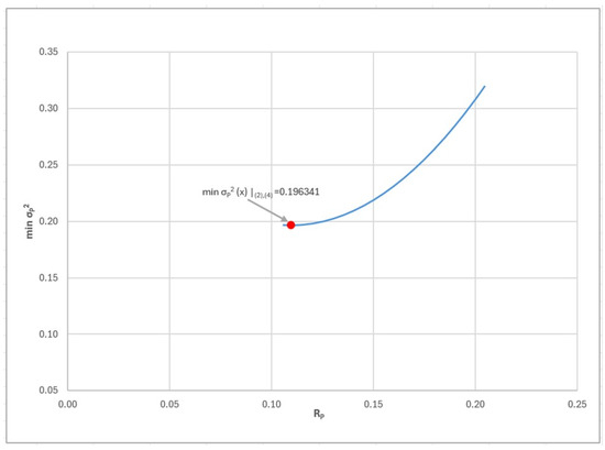
The optimization result for the selected assets is illustrated in Figure 1.

Figure 1. Risk optimization and identification of the global minimum variance portfolio for the six-asset portfolio.

The proposed framework for portfolio risk minimization provides a rigorous analytical tool, though its application requires careful consideration of the input matrix properties. The next example (Example 2) is presented not as a financially feasible scenario but as an algebraic cautionary case. It illustrates how a symmetric matrix that fails to satisfy the property of positive semi-definiteness can lead to non-physical outcomes, such as negative variance. This highlights the necessity of ensuring that $\mathsf{\Sigma }$ is an admissible covariance matrix to maintain the economic validity of the optimization results.

From (6), (8) and (21), it follows that $min{\sigma }_p^2\left(x\right)\ge 0$ exactly when $\left|\mathsf{\Sigma }\right|\ge 0$. In Example 2, we show that for $n=3$, there exist values of the covariations satisfying Inequalities (1) for which $x^{\ast }\in S_n$ but $min{\sigma }_p^2{\left(x\right)|}_{\left(2\right)}={\sigma }_p^2\left(x^{\ast }\right)<0$.

Example 2. 

Let $n=3$. Consider the matrix $\mathsf{\Sigma }=\left(\begin{array}{ccc}0.25& -0.20& -0.30\\ -0.20& 0.36& -0.40\\ -0.30& -0.40& 0.49\end{array}\right).$ Then, Inequalities (1) have the form

$$-0.2>-\sqrt{0.250.36}=-0.3;$$

$$-0.3>-\sqrt{0.250.49}=-0.35\mathit{and}-0.4>-\sqrt{0.360.49}=-0.42.$$

Then $b^T=(0.79,0.89)$, $c=\left(\begin{array}{cc}0.55& 0.20\\ 0.10& 0.76\end{array}\right)$ and the matrix A is in the following form

$$A=\left(\begin{array}{cc}1.34& 0.99\\ 0.99& 1.65\end{array}\right).$$

In confirmation of Lemma 2, Inequalities (16) are valid too:

$$M_1^A=\left|1.34\right|=-\left|\begin{array}{ccc}0.25& -0.3& 1\\ -0.3& 0.49& 1\\ 1& 1& 0\end{array}\right|=1.3400>0;$$

$$M_2^A=\left|\begin{array}{cc}1.34& 0.99\\ 0.99& 1.65\end{array}\right|=-\left|\begin{array}{cccc}0.25& -0.20& -0.30& 1\\ -0.20& 0.36& -0.40& 1\\ -0.30& -0.40& 0.49& 1\\ 1& 1& 1& 0\end{array}\right|=1.2309>0.$$

According to Theorem 3, this guarantees the existence of $min{\sigma }_p^2{\left(x\right)|}_{\left(2\right)}$ in the point $x^{\ast }(x_1^{\ast },x_2^{\ast },x_3^{\ast })$. Additionally,

$$|{\mathsf{\Sigma }}_1|=\left|\begin{array}{ccc}1& -0.20& -0.30\\ 1& 0.36& -0.40\\ 1& -0.40& 0.49\end{array}\right|=0.4224,\left|{\mathsf{\Sigma }}_2\right|=\left|\begin{array}{ccc}0.25& 1& -0.30\\ -0.20& 1& -0.40\\ -0.30& 1& 0.49\end{array}\right|=0.4105,$$

$$|{\mathsf{\Sigma }}_3|=\left|\begin{array}{ccc}0.25& -0.2& 1\\ -0.20& 0.36& 1\\ -0.30& -0.40& 1\end{array}\right|=0.3980,$$

whence, according to Lemma 1, we obtain ${\displaystyle -\left|\begin{array}{cc}\mathsf{\Sigma }& 1\\ 1& 0\end{array}\right|=\sum _{i=1}^3\left|{\mathsf{\Sigma }}_i\right|=1.2309}$,

$$x_1^{\ast }={\displaystyle \frac{|{\mathsf{\Sigma }}_1|}{-\left|\begin{array}{cc}\mathsf{\Sigma }& 1\\ 1& 0\end{array}\right|}}={\displaystyle \frac{0.4224}{1.2309}}\approx 0.3432;x_2^{\ast }={\displaystyle \frac{|{\mathsf{\Sigma }}_2|}{-\left|\begin{array}{cc}\mathsf{\Sigma }& 1\\ 1& 0\end{array}\right|}}={\displaystyle \frac{0.4105}{1.2309}}\approx 0.3335;$$

$$x_3^{\ast }={\displaystyle \frac{|{\mathsf{\Sigma }}_3|}{-\left|\begin{array}{cc}\mathsf{\Sigma }& 1\\ 1& 0\end{array}\right|}}={\displaystyle \frac{0.3980}{1.2309}}\approx 0.3233,$$

and ${\displaystyle \sum _{i=1}^3{x}_i^{\ast }=1}$. However,

$$\left|\mathsf{\Sigma }\right|=\left|\begin{array}{ccc}0.25& -0.20& -0.30\\ -0.20& 0.36& -0.40\\ -0.30& -0.40& 0.49\end{array}\right|=-0.0959,$$

and (21) implies ${\displaystyle min{\sigma }_p^2{\left(x\right)|}_{\left(2\right)}=\frac{\left|\mathsf{\Sigma }\right|}{-\left|\begin{array}{cc}\mathsf{\Sigma }& 1\\ 1& 0\end{array}\right|}=\frac{-0.0959}{1.2309}=-0.0779}$.

According to (9), the function ${\sigma }_p^2$ has the form

$${\sigma }_p^2\left(\tilde{x}\right)=1.34x_1^2+1.98x_1{x}_2+1.65x_2^2-1.58x_1-1.78x_2+0.49.$$

It is continuous in both variables, and therefore there exists a neighborhood of the point $x^{\ast }$ in which it preserves its negative sign. By means of the change in variables

$$\left(\begin{array}{c}{x}_1\\ x_2\end{array}\right)=\left(\begin{array}{c}0.3432\\ 0.3335\end{array}\right)+\left(\begin{array}{cc}0.76& 0.65\\ -0.65& 0.76\end{array}\right)\left(\begin{array}{c}{y}_1\\ y_2\end{array}\right)$$

we obtain

$${\sigma }_p^2\left(y\right)=0.493y_1^2+2.497y_2^2-0.07791.$$

Therefore, in the elliptical region

$${\left({\displaystyle \frac{y_1}{0.39756}}\right)}^2+{\left({\displaystyle \frac{y_2}{0.17664}}\right)}^2\le 1,$$

i.e.,

$${\left({\displaystyle \frac{0.76(x_1-0.3432)-0.65(x_2-0.3335)}{0.39756}}\right)}^2+{\left({\displaystyle \frac{0.65(x_1-0.3432)+0.76(x_2-0.3335)}{0.17664}}\right)}^2\le 1$$

with center at $(0.3432;0.3335)$, the function ${\sigma }_p^2\left(\tilde{x}\right)$ is non-positive.

This example shows that under condition (2), the symmetry of Σ and the validity of Inequalities (1) and (3) are insufficient for the positive definiteness of the quadratic function ${\sigma }_p^2\left(\tilde{x}\right)$ defined in (9). This is an important circumstance which should be kept in mind when this form is used as an empirical variance of a multidimensional random variable.

Remark 3. 

It is important to clarify that “negative portfolio risk” in this context serves as a theoretical diagnostic indicator rather than physical reality. Mathematically, this result signifies that the input covariance matrix Σ is not positive definite. In practical financial applications, such a scenario may occur during periods of extreme market stress, through data asynchronicity, or when assets exhibit perfect multi-collinearity. Within our framework, this finding highlights the boundary conditions of the optimization process. It underscores the necessity of employing regularization techniques, such as the Ledoit–Wolf shrinkage, to ensure that the matrix is well-conditioned and positive definite before deriving real-world investment weights.

To demonstrate the practical utility of the proposed determinant-based identities, in the next example (Example 3), we apply the framework to a portfolio of three highly liquid equity assets: NVIDIA (NVDA), JPMorgan Chase (JPM), and Procter & Gamble (PG). These assets are selected to represent the growth, financial, and defensive sectors, respectively.

Example 3. 

The empirical data for the three risky assets (NVDA, JPM and PG) in this example are retrieved from the Yahoo Finance database. We utilize Adjusted Closing prices, which account for all corporate actions, including dividend distributions and stock splits. The use of adjusted prices is critical for financial modeling as they reflect the true total return to the investor and eliminate artificial price discontinuities.

The dataset spans one full calendar year, from 17 March 2025 to 16 March 2026. Daily frequency is chosen for the observations, providing a sample size of approximately 252 trading days. This frequency ensures statistical robustness and provides sufficient degrees of freedom for the stable estimation of the covariance matrix parameters. The daily rates of return $R_t$ are calculated using the standard discrete (simple) return method: ${\displaystyle R_t=\frac{P_t-P_{t-1}}{P_{t-1}}}$, where $P_t$ represents the adjusted price at day t and $P_{t-1}$ is the price on the preceding trading day. Following the generation of the return series, the following statistical measure is computed: mean daily return $R_{daily}$, calculated as the arithmetic average of the daily returns over the sample period

$$R_{daily}={\displaystyle \frac{1}{n}}\sum _{t=1}^n{R}_t.$$

To convert the daily mean into a standard annual format $R_i(i=1,2,3)$, the daily return is multiplied by the number of trading days in a year:

$$R_i=R_{daily}\times 252.$$

The variance and covariance elements of the covariance matrix Σ are estimated based on daily deviations from the mean. For the final optimization, the matrix is annualized (multiplied by 252) to align with the scale of the annualized returns.

Thus, we consider three capital assets portfolio (NVDA, JPM and PG) with returns $R_1=0.500509$, $R_2=0.226597,$ and $R_3=-0.102961$ of the assets and with the following variance–covariance matrix

$$\mathsf{\Sigma }=\left(\begin{array}{ccc}0.171966& 0.000212& -0.010180\\ 0.000212& 0.064029& 0.000016\\ -0.010180& 0.000016& 0.035620\end{array}\right).$$

The covariance matrix Σ is tested for positive definiteness. The verification step confirmed that all principal minors are positive and that the determinant $\left|\mathsf{\Sigma }\right|=0.0003856>0$ is strictly greater than zero. This step ensures that the empirical data is “physically admissible”, guaranteeing the existence and uniqueness of the global minimum variance portfolio, which is the central focus of this theoretical framework. Then

$$|{\mathsf{\Sigma }}_1|=\left|\begin{array}{ccc}1& 0.000212& -0.010180\\ 1& 0.064029& 0.000016\\ 1& 0.000016& 0.035620\end{array}\right|=0.002925;$$

$$|{\mathsf{\Sigma }}_2|=\left|\begin{array}{ccc}0.171966& 1& -0.010180\\ 0.000212& 1& 0.000016\\ -0.010180& 1& 0.035620\end{array}\right|=0.006009;$$

$$|{\mathsf{\Sigma }}_3|=\left|\begin{array}{ccc}0.171966& 0.000212& 1\\ 0.000212& 0.064029& 1\\ -0.010180& 0.000016& 1\end{array}\right|=0.011658.$$

We obtain ${\displaystyle -\left|\begin{array}{cc}\mathsf{\Sigma }& 1\\ 1& 0\end{array}\right|=\sum _{i=1}^3\left|{\mathsf{\Sigma }}_i\right|=0.020592}$,

$$x_1^{\ast }={\displaystyle \frac{|{\mathsf{\Sigma }}_1|}{-\left|\begin{array}{cc}\mathsf{\Sigma }& 1\\ 1& 0\end{array}\right|}}={\displaystyle \frac{0.002925}{0.020592}}\approx 0.142040;x_2^{\ast }={\displaystyle \frac{|{\mathsf{\Sigma }}_2|}{-\left|\begin{array}{cc}\mathsf{\Sigma }& 1\\ 1& 0\end{array}\right|}}={\displaystyle \frac{0.006009}{0.020592}}\approx 0.291824;$$

$$x_3^{\ast }={\displaystyle \frac{|{\mathsf{\Sigma }}_3|}{-\left|\begin{array}{cc}\mathsf{\Sigma }& 1\\ 1& 0\end{array}\right|}}={\displaystyle \frac{0.011658}{0.020592}}\approx 0.566136.$$

Since

$$\left|\mathsf{\Sigma }\right|=\left|\begin{array}{ccc}0.171966& 0.000212& -0.010179\\ 0.000212& 0.064029& 0.000016\\ -0.010179& 0.000016& 0.035621\end{array}\right|=0.000386,$$

according to (21), it follows that ${\displaystyle min{\sigma }_p^2{\left(x\right)|}_{\left(2\right)}=\frac{\left|\mathsf{\Sigma }\right|}{-\left|\begin{array}{cc}\mathsf{\Sigma }& 1\\ 1& 0\end{array}\right|}=\frac{0.000386}{0.020592}=0.018725}$. Then $min{\sigma }_p{\left(x\right)|}_{\left(2\right)}=\sqrt{min{\sigma }_p^2{\left(x\right)|}_{\left(2\right)}}=0.136838$. From (23) for the weighted average return $R_p^{\ast }$, we obtain

$$R{p}^{\ast }={\displaystyle \frac{\left|\begin{array}{cc}\mathsf{\Sigma }& 1\\ R& 0\end{array}\right|}{\left|\begin{array}{cc}\mathsf{\Sigma }& 1\\ 1& 0\end{array}\right|}}={\displaystyle \frac{-0.001625}{-0.020592}}=0.078929.$$

The results are summarized in Table 1.

Table 1. Empirical optimization results (annualized data).

Statistic	NVDA	JPM	PG	Portfolio (GMVP)
Annualized Expected Return	50.0509%	22.6597%	−10.2961%	7.8929%
Annualized Volatility ($\sigma$)	41.4688%	25.3040%	18.8734%	13.6838%
Optimal Weights ($x_i^{\ast }$)	14.2040%	29.1824%	56.6136%	100%

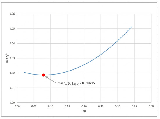
The optimization result for the selected assets is illustrated in Figure 2.

Figure 2. Risk optimization and identification of the global minimum variance portfolio for the three-asset (NVDA, JPM and PG) portfolio.

The analytical solution successfully identified the optimal allocation that minimizes total portfolio risk. As expected, the model assigned the largest weight ($56.6136\%$) to Procter & Gamble (PG), which exhibits the lowest individual volatility, while strategically incorporating NVDA and JPM to exploit diversification benefits through their covariance structure. The portfolio’s expected return of $7.8929\%$ corresponds to the minimum achievable risk level ($\min {\sigma }_p=13.6838\%$) for this asset universe. These results were cross-validated against standard optimization solutions generated via Excel Solver, yielding identical values.

5. Discussion: Data Requirements, Robustness, and Limitations

The practical implementation of the proposed algorithm in real-world investment management requires careful consideration of data inputs and structural stability. A primary challenge in portfolio optimization is the estimation of the variance–covariance matrix $\mathsf{\Sigma }$. In environments with limited or noisy market data, the sample covariance matrix often suffers from estimation error, which can lead to unstable and extreme asset weights.

To enhance the model’s practicality and ensure the stability of input parameters, practitioners can utilize two primary approaches. First, Ledoit–Wolf shrinkage (Ledoit & Wolf, 2004) can be applied to smooth out statistical noise inherent in historical datasets. Second, the adoption of a Factor Model (Chan et al., 1999) enables the framework to capture the fundamental economic logic behind asset dependencies, thereby effectively mitigating the risk of relying on spurious correlations. The proposed algorithm is designed to be fully compatible with these advanced estimation techniques. By integrating a shrinkage estimator or a factor-based covariance matrix as the primary input for $\mathsf{\Sigma }$, the algorithm’s ability to identify the true global minimum variance is significantly enhanced.

However, it is important to note that our model possesses intrinsic robustness even before such refinements due to two fundamental factors:

1.

By isolating the global minimum variance (GMV) portfolio, the model eliminates the need to estimate expected returns—the most volatile and error-prone parameter in the Markowitz framework.

2.

The imposition of non-negative weights does not merely serve as a practical boundary; it acts as a form of implicit regularization Jagannathan and Ma (2003). This significantly reduces the model’s sensitivity to noise and prevents the aggressive shorting of assets that often occurs in unconstrained optimization.

The structural properties of the model indicate that while the optimal weights are influenced by the quality of covariance estimates, the resulting portfolio remains more stable under market stress compared to unconstrained risk–return models.This combination of methodological compatibility and structural robustness ensures that the optimal weights derived are driven by persistent relationships rather than transitory market noise, providing a reliable solution for real-world portfolio construction.

5.1. Comparative Analysis with Alternative Risk Frameworks

While modern frameworks such as CVaR (Conditional Value-at-Risk) and robust optimization offer advanced protection against tail risks and parameter uncertainty, the proposed GMV algorithm provides distinct advantages in specific scenarios.

• Unlike CVaR, which often requires large-scale simulations or linear programming that can be computationally intensive for high-dimensional portfolios, our analytical approach offers computational speed and stability, making it suitable for real-time rebalancing.
• Robust optimization aims to protect against worst-case scenarios but often results in overly conservative portfolios that may sacrifice significant performance. Our model, by focusing on the GMV through the lens of necessary and sufficient conditions, maintains a balance between risk control and practical weight distribution (Table 2).

Table 2. Comparative analysis: proposed GMV model vs. alternative risk frameworks.

Feature	Proposed GMV Model	CVaR Model	Robust Optimization
Objective	Overall Volatility Min.	Tail-Risk Mitigation	Worst-Case Protection
Complexity	Low (Analytical)	High (Simulation-based)	Medium to High
Data Inputs	Covariance Matrix ($\mathsf{\Sigma }$)	Full Distribution	Uncertainty Sets
Scenario	Large-scale Portfolios	Hedge Funds/Tail Risk	High Parameter Instability
Advantage	Direct Analytical Solution	Extreme Market Events	Conservative Buffering

5.2. Future Research Directions and Potential Outcomes

In a forthcoming scientific publication based on the present study, a significant expansion of the current approach is planned, integrating dynamic parameters and a broader analytical scope. The future results will focus on the determination of the efficient set. Following Markowitz’s theory, an approach for identifying the full spectrum of efficient portfolios will be presented. The efficient frontier is determined by establishing the functional relationship between ${\sigma }_p^2$ and $R_p$ subject to conditions

$$\left|\begin{array}{cc}& R_p=\sum _{i=1}^n{x}_i{R}_i\hfill \\ & x_i\left(R_p\right)>0\mathrm{for}\mathrm{all}i=\overline{1,n-2}.\hfill \end{array}\right.$$

This transforms the quadratic form ${\sigma }_p^2\left(x\right)=x^T\mathsf{\Sigma }x$ into a quadratic function ${\sigma }_p^2\left(\tilde{x}\right)$. By applying the necessary condition for the minimum, we obtain ${\displaystyle x_i=\frac{a_i{R}_p-b_i}{c_i}>0}$ ($a_i$, $b_i$ and $c_i$ are real numbers), defining the return constraints for portfolios with short-selling allowed. Within the resulting interval for $R_p$, the endpoints of the efficient set in the portfolios are specified.

In addition, the structural design of the model ensures that even with a static estimation, it maintains reliable stability through non-negative constraints. These constraints act as an inherent filter against noise—a benefit that can sometimes be compromised in more complex, over-parameterized dynamic models. Time-varying volatility can be integrated using a rolling window estimation approach, thus allowing the efficient frontier to adapt to changing market regimes while preserving the model’s structural stability and computational efficiency.

The analysis for $n=2$ assets will illustrate the direct relationship between portfolio risk and expected portfolio return, whereas for $n\ge 3$, the study will focus on the relationship between the global minimum variance (minimum portfolio risk) and the corresponding portfolio return. The results will be organized through precise tabular data representations and graphical mapping, thereby allowing for the full visualization of the efficient frontier.

6. Conclusions

The main elements of Markowitz’s model are based on the expected return and risk of financial instruments. For the first time, Markowitz draws attention not to the number of instruments but to the types of instruments in which one invests and to the interrelationships between them. This logic forms the basis for hedging operations based on capital markets, which aim to minimize the risks of investing in stocks and bonds.

The model proposed in this study for constructing a minimum risk portfolio is characterized by its practical utility and simplified algorithmic structure. By utilizing the classic Markowitz framework, which was adapted through modern software tools (such as Wolfram Mathematica and Excel), precise results are achieved through an uncomplicated yet mathematically rigorous algorithm. The primary advantages of this model for financial analysis include:

• Direct Analytical Solution: By directly employing the variance–covariance matrix for the selected assets, the model avoids the unnecessary complexity typical of large-scale optimization tasks without compromising analytical precision.
• Practical Replicability: The methodology is designed to be easily replicable in a real-world environment, providing investors with a clear visual and numerical representation of the minimum variance portfolio.
• Transparency of Results: The simplified data structure allows for easy verification of each optimization step—from calculating individual sigma ($\sigma$) values to the final testing of portfolio weights ($x_i$).

In conclusion, the model offers a balance between theoretical depth and operational ease, making it a suitable tool for research focused on finding optimal investment solutions under risk conditions in a fast and reliable manner.

References

- Baviera, R., & Bianchi, G. (2021). Model risk in mean variance portfolio selection: An analytic solution to the worst case approach. Journal of Global Optimization, 81, 469–491. [Google Scholar] [CrossRef] [Scilit]
- Bodie, Z., Kane, A., & Marcus, A. J. (2017). Investments (11th ed.). McGraw-Hill Education. [Google Scholar]
- Chan, L. K. C., Karceski, J., & Lakonishok, J. (1999). On portfolio optimization: Forecasting covariances and choosing the risk model. The Review of Financial Studies, 12, 937–974. [Google Scholar] [CrossRef] [Scilit]
- Cheng, T., & Chen, K. (2023). A general framework for portfolio construction based on generative models of asset returns. The Journal of Financial Data Science, 9, 100113. [Google Scholar] [CrossRef] [Scilit]
- Elton, E. J., & Gruber, M. J. (1995). Modern portfolio theory and investment analysis (5th ed.). John Wiley & Sons. [Google Scholar]
- Fabozzi, F. J. (2001). Bond portfolio management (2nd ed.). Frank J. Fabozzi Associates. [Google Scholar]
- Fikhtengol’ts, G. M. (1956). Course of differential and integral calculus (Vol. 1). Fizmatgiz. (In Russian) [Google Scholar]
- Fikhtengol’ts, G. M. (1957). Course of differential and integral calculus (Vol. 2). Fizmatgiz. (In Russian) [Google Scholar]
- Fikhtengol’ts, G. M. (1958). Course of differential and integral calculus (Vol. 3). Fizmatgiz. (In Russian) [Google Scholar]
- Jagannathan, R., & Ma, T. (2003). Risk reduction in large portfolios: Why imposing the wrong constraints helps. The Journal of Finance, 58, 1651–1683. [Google Scholar] [CrossRef] [Scilit]
- Ledoit, O., & Wolf, M. (2004). Honey, I shrunk the sample covariance matrix. The Journal of Portfolio Management, 30, 110–119. [Google Scholar] [CrossRef] [Scilit]
- Li, J., & Xu, M. (2013). Optimal dynamic portfolio with mean CVaR criterion. Risks, 1, 119–147. [Google Scholar] [CrossRef] [Scilit]
- Lintner, J. (1965). The valuation of risk assets and the selection of risky investments in stock portfolios and capital budgets. The Review of Economics and Statistics, 47, 13–37. [Google Scholar] [CrossRef] [Scilit]
- Markowitz, H. (1952). Portfolio selection. The Journal of Finance, 7, 77–91. [Google Scholar] [PubMed]
- Markowitz, H. (1959). Portfolio selection: Efficient diversification of investments. John Wiley & Sons. [Google Scholar]
- Patev, P., & Kanaryan, N. (2008). Portfolio management. Publishing House “ABAGAR”. (In Bulgarian) [Google Scholar]
- Razak, H. N. A., Maasar, M. A., Hafidzah, N. H., & Lee, E. S. C. (2019). Portfolio optimization of risky assets using mean variance and mean CVaR. Journal of Academia, 7, 1–12. [Google Scholar]
- Reilly, F. K., & Brown, K. C. (2002). Investment analysis and portfolio management (7th ed.). South-Western College Publications. [Google Scholar]
- Rigamonti, A. (2020). Mean variance optimization is a good choice, but for other reasons than you might think. Risks, 8, 29. [Google Scholar] [CrossRef] [Scilit]
- Senescall, M., & Low, R. K. Y. (2024). Quantitative portfolio management: Review and outlook. Mathematics, 12, 2897. [Google Scholar] [CrossRef] [Scilit]
- Sharpe, W. F. (1963). A Simplified model for portfolio analysis. Management Science, 9, 277–293. [Google Scholar] [CrossRef] [Scilit]
- Sharpe, W. F. (1964). Capital asset prices: A theory of market equilibrium under conditions of risk. The Journal of Finance, 19, 425–442. [Google Scholar]
- Sharpe, W. F. (1967). A linear programming algorithm for mutual fund portfolio selection. Management Science, 13, 499–510. [Google Scholar] [CrossRef] [Scilit]
- Tobin, J. (1958). Liquidity preference as behavior towards risk. The Review of Economic Studies, 25, 65–86. [Google Scholar] [CrossRef] [Scilit]
- Wang, X. (2022). Portfolio optimization of five stocks based on the mean variance model. BCP Business & Management, 35, 687–693. [Google Scholar] [CrossRef] [Scilit]
- Zhang, Y., Li, X., & Guo, S. (2018). Portfolio selection problems with Markowitz’s mean–variance framework: A review of literature. Fuzzy Optimization and Decision Making, 17, 125–158. [Google Scholar] [CrossRef] [Scilit]
- Zhou, J., Liu, C., & Liang, B. (2025). Portfolio optimization based on quadratic programming: A comparative risk return analysis with mean variance model under different time periods. Financial Economics, 3, wdzyjh14. [Google Scholar] [CrossRef] [Scilit]
Disclaimer/Publisher’s Note: The statements, opinions and data contained in all publications are solely those of the individual author(s) and contributor(s) and not of MDPI and/or the editor(s). MDPI and/or the editor(s) disclaim responsibility for any injury to people or property resulting from any ideas, methods, instructions or products referred to in the content. |
© 2026 by the authors. Licensee MDPI, Basel, Switzerland. This article is an open access article distributed under the terms and conditions of the Creative Commons Attribution (CC BY) license.