


Abstract
This study examines whether speculative bubbles in cryptocurrency markets are transmitted to the assets that finance the energy transition, or whether both segments respond to common drivers. Using freely available weekly and daily data from January 2020 to September 2026, it applies the generalised sup ADF procedure with Monte Carlo and wild-bootstrap critical values, separates global explosiveness, exploratory local crossings and independently validated bubbles, and benchmarks the dating against ex-ante log-periodic power-law singularity (LPPLS) diagnostics and ε-drawdown target events. Synchronisation, causality and dynamic probit tests are calibrated by circular-shift, bootstrap and simulation designs and conditioned on measured common factors. Only Bitcoin’s 2020–2021 run-up survives family-wise control; validated bubbles occur in Bitcoin, Ether and clean-energy equities in 2020–2021 and in battery equities in 2025–2026. Crypto and clean-energy exuberance overlapped in a single joint episode, but the overlap is not significant after multiplicity correction, and no specification shows crypto exuberance predicting green exuberance; the 2017 crypto bubble and the 2024 crypto exuberance had no green counterpart. Detection power is limited and lead–lag orderings are not robust. The evidence rejects crypto-to-green contagion but does not identify a common driver, and is best read as a descriptive account of one shared episode.
Keywords:
speculative bubbles; explosive behaviour; GSADF; LPPLS; cryptocurrencies; clean energy; carbon allowances; co-explosivity JEL Classification:
C22; C15; G12; G14; G15; Q42
1. Introduction
The interplay between speculative dynamics in cryptocurrency markets and the valuation of energy-transition assets has gained growing attention as both segments experienced extraordinary price surges and collapses in recent years. Between late 2020 and early 2021, Bitcoin more than tripled in value, while clean-energy and solar equity indices rose by 30–60% in a matter of weeks, and this sequence was followed by sharp reversals in 2021–2022. A similar pattern of rapid appreciation re-emerged around the approval of US spot Bitcoin exchange-traded funds in early 2024 (Babalos et al., 2025; Liu & Yang, 2024). At the same time, green finance has reached a systemic scale, with cumulative aligned sustainable debt of approximately USD 6.8 trillion by the end of 2025 (Climate Bonds Initiative, 2026). Speculative bubbles in assets that finance the energy transition are not a mere curiosity. Overvaluation can misallocate capital towards projects whose financing collapses once exuberance fades, and a subsequent crash can raise the cost of capital for the transition precisely when long-term investment is needed (Lehnert, 2023; Potrykus et al., 2024). Understanding whether such episodes originate in, or are transmitted from, highly speculative crypto markets is therefore important for investors, regulators and climate-finance policymakers.
Importantly, the various energy-transition segments differ in their potential for speculative overvaluation. Clean-energy and solar equities are growth-oriented and highly sensitive to expectations about policy support and technological adoption, which makes them prone to valuation surges when climate optimism rises (Igeland et al., 2024; Pástor et al., 2022). Battery-technology and lithium-related equities are tied to critical-minerals markets that have themselves displayed bubble behaviour (X.-Q. Wang et al., 2023). EU carbon allowances are policy-created assets whose prices have repeatedly shown explosive episodes linked to market reforms, energy shocks and speculative positioning (Huang & Wang, 2024; Wei et al., 2022), and whose pricing is tied to the financing conditions of polluting firms (Azzone et al., 2025). Green bonds, by contrast, are high-grade fixed-income instruments whose valuations are anchored by interest rates rather than by growth expectations (Mertzanis & Tebourbi, 2025; Sheenan, 2023). The Brent oil benchmark reflects the conventional energy system where its price cycle is sensitive to geopolitical surprises and transfers to the green energy market (Chishti et al., 2023; Elsayed et al., 2024; Maneejuk et al., 2024). The above differences suggest that, if any, exuberance will have heterogeneous impacts on transition assets. Related evidence from crude oil and currency markets also documents changing cross-market spillover patterns across crisis periods (Almansour et al., 2024).
Two explanations compete for the co-movement of these speculative episodes. According to the contagion approach, enthusiasm in one market gets transferred to the other through wealth effects, portfolio adjustment and common investors; hence, a crypto bubble must come before a green bubble (Chen et al., 2024; Escobari & Sharma, 2026). In a common-driver account, both segments are long-duration claims on uncertain future adoption whose valuations respond to the same discount-rate, liquidity and narrative shocks, so that their explosive regimes can coincide without any transmission (Gordo et al., 2024; Pástor et al., 2022; P. Zhang et al., 2024). Section 2 develops this argument and derives testable implications that discriminate between the two accounts. This question is particularly relevant because the crypto and green segments are increasingly linked through investors and narratives: recent work documents strong interdependence between cryptocurrencies, clean energy and green markets, especially during the COVID-19 period (Arfaoui et al., 2023; Mensi et al., 2025), shifting transmission roles around the Russia–Ukraine conflicts (Patel et al., 2023), and growing links through environmental attention and climate-policy uncertainty (Ding et al., 2025; Qing et al., 2025), as well as through the energy footprint of crypto mining (Ali et al., 2024; Kumari et al., 2024; Ren & Lucey, 2022). Research on green cryptocurrencies and sustainable-finance assets also finds pronounced downside-tail connectedness between digital and traditional sustainable assets (Almansour et al., 2026).
While the existing literature has examined bubbles in each of these markets, the evidence remains fragmented. In crypto markets, M’bakob (2024) shows that Bitcoin and Ether bubbles recur in cycles linked to Bitcoin halvings; Oldani et al. (2025) date-stamp multiple explosive episodes in Bitcoin and Ether between 2018 and 2024, linking them to halving events, the pandemic and changing expectations, and showing that restrictive monetary policy burst both bubbles in 2024. Osman et al. (2024) find that crypto-market fear and greed sentiment drive price bubbles, and Chen et al. (2024) show that large cryptocurrencies such as Bitcoin and Ether generate co-bubbles in smaller clean and dirty cryptocurrencies. In green markets, Potrykus et al. (2024) document price bubbles and co-bubbles in solar and wind indices, with peaks during COVID-19 and the Russia–Ukraine conflicts, and Lehnert (2023) argues that explosive movements in green stocks started roughly a year before the broader US market bubble of 2021. Foglia and Miglietta (2024) show that ESG sentiment amplifies positive bubbles in ESG markets, while Huang and Wang (2024) and Wei et al. (2022) identify multiple bubbles in global emission trading schemes, with the EU ETS displaying the highest frequency. Ariza and Ferrer (2025) identify speculative exuberance in renewable energy equities in the US, Europe and China beginning in late 2020, but find limited co-explosivity with broader stock markets, while Franco et al. (2026) report strong evidence of bubble dynamics in renewable-energy indices driven by policy incentives and investor flows, and Vriz and Grossi (2026) conceptualise green bubbles as a potentially “necessary evil” of the transition that may nonetheless culminate in “Climate Minsky” moments. Zheng and Lucey (2025) show that media sentiment, rather than fundamentals, is the most robust driver of clean-energy stock prices, and Qiao et al. (2024) find that climate policy uncertainty is a critical node in risk transmission among clean energy and energy metals. The case of the lithium industry is that of X.-Q. Wang et al. (2023), who demonstrate bubble contagion along the supply chain, while Li et al. (2025) reveal that global economic growth and depreciation of the dollar make commodity price bubbles more probable. Outside of these markets, Escobari and Sharma (2026) confirm that contagion in G7 stock markets becomes more likely during crises than during bubbles, while X. Wang et al. (2026) demonstrate that bubbles in Chinese stock markets spread from leading to other sectors and predate instabilities, and Yang and Ferrer (2023) confirm significant movement of explosive periods between Chinese equity sectors. With regard to the crypto asset markets, Bazán-Palomino (2022) demonstrates reduced interdependence among major cryptocurrencies during bubble periods and increased contagion after these bubbles pop up.
Two further strands bear directly on the present design. First, the dating of explosive episodes is method-dependent. The recursive one-sided test aims at a slightly explosive autoregressive model as an alternative hypothesis but shows size distortions and lack of power under leverage effects and other types of alternative bubbles (Monschang & Wilfling, 2021), while LPPLS is aimed at a super exponential growth regime and provides a distribution of critical times (Filimonov & Sornette, 2013; Johansen & Sornette, 1998). Comparisons using two centuries of S&P 500 data (Q. Zhang et al., 2016), on Bitcoin (Geuder et al., 2019), on carbon markets (Huang & Wang, 2024) and on simulated data (Bertelsen, 2020) show that the two approaches carry complementary information, with BSADF tending to produce longer episodes and LPPLS shorter ones. Second, closely related work on the assets examined here combines LPPLS with independent benchmarks. Giorgis et al. (2024) dissect the 2004–2008 clean-tech bubble, combining LPPLS with social and narrative evidence and a test of clean-tech performance relative to the broad equity market; Wheatley et al. (2019) evaluate Bitcoin bubbles against a network-based valuation benchmark; Gerlach et al. (2019) classify Bitcoin drawups and drawdowns at multiple scales and construct independently observable target events; and Huber and Sornette (2022) interpret Bitcoin bubbles as self-reinforcing adoption cycles that may accelerate innovation. All these contributions taken together indicate that any valid empirical study of coexplosions between cryptos and environmental factors has to verify the statistical signals against independent definitions of bubbles.
In this context, there are still three gaps, each of which is relevant for its own reasons. First, to date, no literature has attempted to establish dates for explosive periods in the main cryptocurrency assets, as well as the entire range of transition assets, including carbon allowances, green bonds, and clean-energy and battery technology stocks. The relevance of this gap is in the fact that the question of leadership and thus the direction of the supervisory reaction depends on comparing the dates in these markets. Second, the co-bubble literature typically infers transmission from co-occurrence, without distinguishing synchronised exuberance driven by common factors from contagion in which one market’s bubble causes another’s. This is important because both explanations have opposite implications: in the case of contagion, limiting the euphoria of crypto would safeguard transition finance, while in the case of common drivers, this would not address the reason for both being overvalued. Third, the consequences of bubble collapses for transition assets, and whether the institutionalisation of crypto through spot exchange-traded funds in 2024 created a channel to green markets that was absent in 2020–2021, remain largely unexplored. This matters because a structural link would change the risk profile of sustainability-oriented portfolios, and because post-bubble drawdowns in clean-energy equities raise the cost of equity for transition firms. This study addresses these gaps by asking whether crypto bubbles are transmitted to energy-transition assets, or whether both segments are driven by a common speculative cycle.
Methodologically, the study combines the generalised sup ADF (GSADF) procedure of Phillips et al. (2015a, 2015b) with finite-sample Monte Carlo and heteroskedasticity-robust wild-bootstrap critical values (Harvey et al., 2016), and separates three objects: global evidence of explosiveness, exploratory local crossings of the backward SADF (BSADF) statistic, and economically meaningful bubbles that are validated independently by ex-ante LPPLS diagnostics and subsequent ε-drawdowns (Filimonov & Sornette, 2015; Johansen & Sornette, 2001). It compares GSADF and LPPLS at every historical cutoff against independently defined target events, calibrates size and power by simulation, and tests transmission using positive-state overlap measures with circular-shift nulls, Toda–Yamamoto tests between BSADF sequences (Toda & Yamamoto, 1995) calibrated by bootstrap, harmonised dynamic probit models with block-bootstrap inference, and a model with measured common factors. Figure 1 summarises the research design.
Figure 1.
Research design. Notes: The above figure shows the six steps involved in the empirical methodology, from data construction through global explosiveness tests to episode classification and independent benchmark tests. The curved arrow from Step 3 to Step 4 indicates that tier (iii) episodes are classified only after the independent validation carried out in Step 4.
The findings are graded by the strength of the evidence. Apart from an explosive decline in green bonds, only Bitcoin rejects the null of no explosiveness at the 5% level with heteroskedasticity-robust critical values, and only its 2020–2021 run-up exceeds a family-wise threshold among the exuberance episodes. Independently validated bubbles are confined to Bitcoin, Ether and two clean-energy indices in 2020–2021 and to battery-technology equities in 2025–2026, whereas the explosive episodes in carbon allowances and green bonds do not display the speculative signature. Crypto and clean-energy exuberance coincided in a single joint episode in December 2020–February 2021; the overlap is not significant once multiplicity is controlled, lead–lag orderings change across reasonable dating choices, and no specification shows crypto exuberance predicting green exuberance, either unconditionally or conditional on measured common factors. The bubble in Bitcoin prices that happened in 2017, and the crypto enthusiasm triggered by the approval of spot ETFs in 2024, were not paralleled in any way by developments in the cleantech market. Thus, the data does not provide support for any contagion between cryptocurrencies and green investments. It also fails to provide an explanation, as the analysed factors account for virtually nothing about timing.
The remainder of this paper is structured as follows. Section 2 develops the theoretical framework and hypotheses, Section 3 presents the methodological approach, Section 4 describes the data and summary statistics, Section 5 discusses the empirical findings and robustness checks, and Section 6 concludes the study.
2. Theoretical Framework and Hypotheses
2.1. Explosiveness, Bubbles and Fundamentals
Rational bubble theory implies that, if an asset price contains a component that grows at the required rate of return, the log price departs from unit-root behaviour towards explosive dynamics (Diba & Grossman, 1988; Phillips et al., 2015a). The converse does not hold. A statistically explosive segment may reflect a rapid change in fundamentals, a policy or market-design shock, or a correction in the direction opposite to exuberance, and a positive-feedback bubble need not display a constant explosive autoregressive coefficient over the short windows on which recursive tests operate (Johansen & Sornette, 1998; Monschang & Wilfling, 2021). This paper therefore treats an explosive episode as a candidate and reserves the term speculative bubble for episodes that combine (a) explosive dynamics, (b) a faster-than-exponential acceleration of the type captured by LPPLS, and (c) a subsequent large drawdown that is defined independently of either detector. The definition of the three features connects the statistic with the economy, while differentiating the explosive retracements, such as the repricing of high-quality bonds when money is tightened, from the speculative excesses. Accordingly, the term “bubble” is reserved for episodes that satisfy all three criteria (tier (iii) in Section 3.2); other statistically explosive segments are described as explosive episodes or periods of exuberance, because fundamental explanations—such as policy changes, post-pandemic reopening or physical supply–demand shifts in carbon and oil markets—cannot be ruled out for them.
2.2. A Common Valuation-Factor Argument
The argument in the paper itself relies on three properties common to both crypto assets and clean-technology equities. Firstly, both types of assets represent claims of long duration. Cryptocurrency claims generate no contractual cash flows, while the cash flows associated with clean-energy, solar, and battery companies take place in the distant future and require adoption and regulatory support, making valuations of both kinds highly sensitive to the real discount rate and liquidity expectations, as shown in Pástor et al. (2022) for green equities and in Gordo et al. (2024) for renewable-energy stocks under alternative monetary regimes. Secondly, both are subject to pricing based on adoption stories—digital revolution and energy transition—such that an increase in the probability of rapid adoption causes an increase in the value of both (Huber & Sornette, 2022; Shiller, 2017). Thirdly, both are attracting investor attention and momentum traders, who are known to cause positive feedback, turning a common valuation shock into an accelerating process (Foglia & Miglietta, 2024; Koch & Dimpfl, 2023; Osman et al., 2024).
Thus, four theoretical approaches serve different purposes within one argument. The rational bubble theory specifies the nature of the statistical object; the global liquidity and discount rate channel gives the common shock; investor attention and sentiment provide the amplification mechanism that transforms the shock into explosive dynamics; and contagion provides the competing explanation. According to the argument, a decline in the real yield rate, an increase in the central bank liquidity, or a change in the narratives of disruption can cause both segments to enter into the regime of explosiveness within a short period of time without any transmission between them. Since investor populations, trading times, and reactions to the shock vary, the reaction is delayed in such a way that originations differ by weeks even without leading markets.
2.3. The Rival Contagion Argument
Contagion means that the excitement in the lead market increases the likelihood of excitement in the follower market beyond the one due to normal circumstances. Wealth effects stemming from gains in crypto assets, portfolio rebalancing by the investors holding both markets, and attention spillovers due to media coverage of the crypto asset rally are possible mechanisms for contagion (Chen et al., 2024; Escobari & Sharma, 2026). In the line of Forbes and Rigobon (2002), co-movements that are left even after conditioning on common shocks are defined as contagion, while those that are driven by common shocks are interdependence.
2.4. Testable Implications
These arguments have four implications, which are summarised in Table 1 below. H1 (prediction directionality): Under crypto-to-green contagion, lagged crypto exuberance predicts green exuberance conditional on common factors and the size of the effect is greater than that of the reverse effect; under the common drivers argument, cross-market effects are zeroed out conditional on the factors, and any unconditional association is symmetric. H2 (dating sequence): Contagion implies that crypto originations happen before green originations regardless of dating decisions, while a common driver implies no sequencing other than measurement error. H3 (bubble recurrence): Contagion implies that there is green exuberance after crypto bubbles, while a common driver implies that recurrent joint exuberances are only possible when the common valuation conditions recur. The 2017 Bitcoin bubble and 2024 spot-ETF episode are out-of-sample predictions to test the hypotheses. H4 (asymmetric aftermath): Contractual cash flow and policy fundamentals—green bonds, carbon allowances and oil—do not show the speculative nature of an identified bubble even if their prices become explosive, while long duration growth assets may.
Table 1.
Theoretical implications and empirical tests.
Implications vary in terms of what they allow us to identify. While rejection of H1 implies rejection of the crypto-to-green contagion channel, the absence of a cross-market effect does not imply the identification of a common factor because it has to be measurable and drive the simultaneous occurrence.
3. Methodological Approaches
The study adopts a multi-stage approach for the analysis of explosive behaviour and its spread through cryptocurrency and energy transition markets. The first stage consists of GSADF testing, which identifies the presence of explosive behaviour and dates the origin and end date of each episode and divides each such episode into one of three degrees of evidence. The second stage involves LPPLS diagnostics and ε-drawdown target events independently identified as an out-of-sample benchmark, with simulation-based calibration of size and power. In the third stage, positive state overlaps, calibrated causality tests, and dynamic probit models with common factor adjustment are adopted to distinguish synchronised exuberance from contagion. All the above-mentioned tests were implemented using Python 3.13 with just-in-time compilation.
3.1. Recursive Explosiveness Tests
Following Phillips et al. (2011) and Phillips et al. (2015a), explosive behaviour is detected through right-tailed recursive ADF regressions on the log price yt. For a sample window starting at fraction r1 and ending at fraction r2 of the full sample, the regression is
and ADFr1r2 denotes the t-statistic of βr1,r2. Under the null hypothesis of a unit root with mild drift, β = 0, whereas explosive behaviour implies β > 0. The generalised sup ADF statistic of Phillips et al. (2015a) is obtained by varying both the starting and ending points of the window over all feasible ranges:
where r0 is the minimum window, set to r0 = 0.01 + 1.8/√T as recommended by Phillips et al. (2015a). This flexibility allows the detection of multiple, recurring bubbles, which the earlier SADF test may miss. The empirical relevance of this procedure is supported by its increasing use in recent studies. For instance, Huang and Wang (2024) applied SADF and GSADF tests to identify price bubbles in six global carbon markets, and Oldani et al. (2025) used recursive unit-root testing to date-stamp collapsing bubbles in cryptocurrencies.
Critical values are obtained in two ways. First, finite-sample critical values are simulated from 2000 Monte Carlo replications of a random walk with drift T−1, matching the sample size and lag order (400 replications for the daily sample). Second, because financial returns display strong volatility clustering that can distort the size of right-tailed tests, heteroskedasticity-robust p-values are obtained from 499 replications of a wild bootstrap with Rademacher weights applied to the demeaned price changes, in the spirit of Harvey et al. (2016). The baseline uses weekly data with k = 1; robustness checks use k = 0 and daily data.
This procedure is well founded for its own statistical alternative. The canonical local alternative is the mildly explosive autoregression
(Phillips et al., 2015a, 2015b). A positive-feedback bubble, however, need not present a constant explosive coefficient over short windows; it may involve accelerating growth, intermittent corrections and changes in risk-taking, and the relation to the subsequent drawdown matters. Monschang and Wilfling (2021) report size distortions under leverage effects, low power against flexible rational-bubble specifications and sensitivity to observation frequency, and Bertelsen (2020) shows in simulations that the size and power of sup ADF and LPPL procedures depend on the null model and on implementation choices. For these reasons, a BSADF flag is treated here as a candidate rather than an unambiguous bubble label (Section 2.1), and the size and power of the procedures used are calibrated by simulation (Section 3.5).
3.2. Date-Stamping and Classification of Explosive Episodes
To date-stamp episodes, the backward SADF (BSADF) statistic is computed for each observation r2 by fixing the window end and varying the start:
The origination of an episode is the first observation at which the BSADF exceeds its 95% critical value, and its termination is the last observation before it falls below the critical value:
where the minimum duration δlog(T), with δ = 1, equals five weeks for the weekly sample and seven trading days for the daily sample. Because the right-tailed test detects explosive dynamics regardless of direction, each episode is classified as exuberance if prices rose over the episode and as an explosive decline if they fell. A negative explosive correction, such as an interest-rate-induced decline in high-grade bonds, is therefore never treated as a speculative bubble.
Because a pointwise crossing over many overlapping windows is not a globally controlled discovery, episodes are classified into three tiers. Tier (i) is global evidence of right-tailed explosiveness: the GSADF statistic exceeds its wild-bootstrap 95% critical value. Tier (ii) comprises exploratory local episodes, in which the BSADF exceeds its pointwise Monte Carlo 95% critical value for at least the minimum duration. To address the episode-level false-discovery problem, a tier (ii) episode is additionally flagged as family-wise significant (FWER) when its peak BSADF exceeds the 95% quantile of the bootstrap distribution of supt BSADFt, which coincides with the bootstrap GSADF critical value. By construction, the probability that any crossing of this threshold occurs anywhere in the sample under the null is 5%, which makes it the full-sample analogue of the multiplicity-controlled monitoring threshold of Phillips and Shi (2020). Local dates are interpreted conditionally on the global test: for an asset without tier (i) evidence, tier (ii) episodes are reported as exploratory and are not used to support claims that require a bubble. Tier (iii) comprises economically meaningful speculative bubbles, namely tier (ii) exuberance episodes that are validated independently by (a) an ex-ante LPPLS positive-bubble signal (confidence indicator of at least 0.10) in some week between 13 weeks before origination and termination, and (b) an independently defined target event—the peak that precedes an ε-drawdown of at least 20%—between origination and 13 weeks after termination (Section 3.3 and Section 3.4). As a robustness check, all episodes are re-dated with asset-specific pointwise wild-bootstrap 95% critical values.
3.3. LPPLS Benchmark
The LPPLS model describes a positive-feedback bubble as a faster-than-exponential trend decorated by log-periodic oscillations that converge on a critical time tc (Filimonov & Sornette, 2013; Johansen & Sornette, 1998). With τ = |tc − t| and 0 < m < 1,
A positive bubble requires B < 0; the accelerating trend is visible even when the oscillatory terms vanish, because d2E[lnP]/dt2 = Bm(m − 1)τm−2 > 0 for B < 0 and 0 < m < 1. The model is calibrated with the stable scheme of Filimonov and Sornette (2013): the linear parameters (A, B, C1, C2) are concentrated out by least squares, and the nonlinear parameters are estimated by a grid search with three refinement rounds over tc ∈ [t2 − 0.2dt, t2 + 0.2dt], m ∈ [0.01, 0.99] and ω ∈ [2, 15], where dt = t2 − t1 is the window length. Following Q. Zhang et al. (2016), a fit is qualified when tc ∈ [t2 − 0.05dt, t2 + 0.1dt], the number of oscillations (ω/π)ln|(tc − t1)/(tc − t2)| is at least 2.5 and the damping ratio m|B|/(ω|C|) is at least 0.5, where |C| = (C12 + C22)1/2. The positive-bubble confidence indicator at week t2 is the share of 14 window lengths (26 to 104 weeks in steps of six) whose fit is qualified with B < 0. All windows end at t2 and use only data available at that date, so the indicator is strictly ex ante; where pre-2020 history exists (Bitcoin from 2015, Ether from 2016, the clean-energy proxies from 2005 to 2008, LIT from 2010), windows may extend into it. The indicator is computed for BTC, ETH, ECO, CELS, SUN, LIT and EUA. The alert threshold of 0.10 and all filter settings were fixed before scoring, and thresholds of 0.05 and 0.20 are reported as sensitivity checks.
3.4. Independent Target Events and Horse Race
Target events are constructed from prices alone, independently of either detector, using the ε-drawdown methodology (Filimonov & Sornette, 2015; Gerlach et al., 2019; Johansen, 2003; Johansen & Sornette, 2001). Starting from a local peak, a drawdown continues as long as no rebound from its running minimum exceeds εt = ε0σt, where σt is the standard deviation of weekly log returns over the preceding 26 weeks; drawups are defined symmetrically. A target event is the peak that precedes an ε-drawdown of at least 20% with ε0 = 2. Because the choice of ε0 and of the magnitude threshold is arbitrary, results are reported for ε0 ∈ {1, 2, 3} and magnitudes of 15%, 20% and 30%. An ex-post event set of this kind is legitimate for scoring forecasts because its definition does not favour either detector.
Four alert rules are compared at every historical cutoff: (1) GSADF with pointwise Monte Carlo critical values, which raises an alert when the BSADF exceeds its 95% critical value and the 13-week return is positive; (2) the same rule with pointwise wild-bootstrap critical values, which uses the full-sample bootstrap and is therefore not strictly ex ante; (3) an LPPLS alert when the positive-bubble confidence indicator is at least 0.10; and (4) a persistence (momentum) baseline that raises an alert when the trailing 13-week return exceeds the 90th percentile of its expanding history. A target is hit when at least one alert occurs between 13 weeks and one week before the peak, and the lead time is measured from the first such alert. An alert run is counted as a false alarm when no target peak occurs during the run or within 13 weeks after it ends. Scoring starts once the BSADF is available (11 September 2020) and covers BTC, ETH, ECO, CELS, SUN, LIT and EUA.
3.5. Simulation Calibration of Size and Power
Size and power are calibrated under explicit data-generating mechanisms with T = 352 weekly observations, matching the empirical sample. Two null designs contain no bubble: (a) a random walk with GJR-GARCH(1,1) innovations, leverage and Student-t(5) shocks (unconditional weekly volatility 4.5%); and (b) a regime-switching drift process in which a Markov chain alternates between weekly drifts of +1.5% and −1.0% with persistence 0.96, representing fundamental repricing without a bubble. Two alternatives contain a bubble with a known target time τ: (c) a mildly explosive autoregression in the log-price deviation, with coefficient 1 + T−0.6 over 40 weeks from a random origination, followed by a collapse over six weeks; and (d) an LPPLS positive-feedback bubble over 60 weeks (m = 0.5, ω = 8, total rise of 100%) with AR(1) noise, followed by a 35% crash over three weeks. Two further two-asset designs examine whether the transmission tests of Section 3.6 can distinguish (e) a common explosive factor loaded with heterogeneous delays of zero to four weeks from (f) directed transmission, in which the explosive component of the second asset is driven by lagged changes in the explosive component of the first. For replication m = 1, …, M, let Wm = 1 if the method raises an alert at least one week before τ within the 13-week evaluation window, and zero otherwise; empirical power is
False-alarm rates are reported as the share of null replications with any alert and as the share of weeks in alert, alongside lead times and the share of bubble replications with alerts more than 13 weeks before τ. Because the LPPLS calibration is computationally intensive, M = 100 for designs (a)–(d), with the confidence indicator evaluated every third week using the same 14 windows and filters as in the empirical analysis, and M = 200 for designs (e)–(f).
3.6. Synchronisation, Causality, Dynamic Probit and Common-Factor Models
To examine whether explosive episodes are shared across markets, this study first computes the concordance index of Harding and Pagan (2006) between the exuberance indicators Sc,t of crypto-asset c and Sg,t of transition asset g:
Because the concordance index is dominated by weeks in which neither series is exuberant, the analysis focuses on the positive-state Jaccard overlap
together with the conditional overlap probabilities Pr(Sg = 1 | Sc = 1) and Pr(Sc = 1 | Sg = 1) and the number of distinct joint episodes. Statistical significance is assessed against a null that preserves the length and clustering of each series’ regimes: one indicator is shifted circularly against the other over all T − 1 offsets, and the p-value is the share of shifts with an overlap at least as large as the observed one. The Holm (1979) correction controls the family-wise error rate across the 14 crypto–transition pairs. The exercise is repeated with wild-bootstrap-dated labels, with LPPLS-based labels (confidence ≥ 0.10), and with labels from BSADF tests on benchmark-relative prices
where Pbroad is a matched broad benchmark (the S&P 500 for ECO and CELS, the MSCI ACWI for SUN and LIT, and the NASDAQ-100 for BTC and ETH), so that growth-stock and discount-rate shocks common to the broad market are removed.
Synchronisation, however, does not imply transmission. To test whether exuberance in one market predicts exuberance in another, the study applies the Toda–Yamamoto causality test (Toda & Yamamoto, 1995) to the BSADF sequences, which measure the time-varying intensity of explosiveness. A bivariate VAR in levels with p + 1 lags is estimated, where p is selected by the AIC, and a Wald test with heteroskedasticity-robust standard errors is applied to the first p lags of the causing variable. The BSADF sequences are, however, generated statistics—recursive extrema of highly overlapping regressions with a non-standard dependence structure—so the nominal Wald distribution is not guaranteed. The null distribution is therefore calibrated by simulation: in each of 499 replications, both price series are generated independently by the wild bootstrap under the unit-root null, both BSADF sequences are reconstructed, and the entire lag-selection, VAR and Wald procedure is rerun; the bootstrap p-value is the share of replications whose asymptotic p-value is at least as small as the observed one. Diagnostics comprise ADF tests on the BSADF sequences, Ljung–Box tests on the VAR residuals and the range of p-values across lag orders one to four. Non-rejections are interpreted as inconclusive rather than as evidence that transmission is absent.
Finally, dynamic probit models estimate the probability that an asset is in an exuberance regime as a function of its own lagged regime, the lagged exuberance regime of the other block and common conditions:
where Sj indicates exuberance in any asset of the other block and X is either ln VIX or the measured common factors defined below. To make the two directions comparable, the design is harmonised: the clean-energy and battery block (ECO, CELS, SUN, LIT) is regressed on lagged crypto exuberance (BTC or ETH), and the crypto block is regressed on lagged clean-energy or battery exuberance, using identical weekly dates (18 September 2020 to 25 September 2026, 315 weeks), identical controls and asset fixed effects. Assets without any exuberance week under a given labelling are dropped because they carry no within-asset variation. The estimand is the average marginal effect of the lagged cross-market regime,
where ηi,t is the index excluding the cross-market term and Φ is the standard normal cdf. Coefficient standard errors are clustered by week. Confidence intervals for the average marginal effects, and a formal test of directional asymmetry, are obtained from a moving-block bootstrap of weeks (block length eight weeks, 499 replications; Künsch, 1989) that resamples the same weeks for both panels. Each model is compared with a baseline that contains only the own lag and controls, using likelihood-ratio tests, the increment in pseudo-R2, the area under the ROC curve (AUC), and expanding-window out-of-sample Brier and log scores from January 2022.
Symmetric predictive effects are not sufficient to identify a common driver, because contemporaneous shocks observed at slightly different market-clock times, feedback in both directions, shared investors, different detection thresholds or a latent factor with heterogeneous delays can all produce them. The common-driver hypothesis is therefore tested directly with measured time-varying factors. Seven weekly indicators capture the drivers named in Section 2: ln VIX (risk appetite), the 10-year real Treasury yield (the growth-stock discount rate), the 13-week change in the two-year Treasury yield (expected policy rates), the 26-week log change in Federal Reserve total assets (central-bank liquidity), the Moody’s Baa–Treasury spread (credit conditions), the 13-week log change in the broad US dollar index, and the 13-week log return of the NASDAQ-100 (the technology and growth-equity cycle). The first two principal components of the standardised indicators, F1 and F2, enter the probit models and the following model for the continuous explosiveness intensities Zi,t = BSADFi,t:
estimated by OLS with HAC standard errors (eight lags) for each crypto–clean-energy pair in both directions. The common-driver hypothesis implies γij = 0 once Ft is controlled for, whereas contagion from crypto implies γij > 0 for j ∈ {BTC, ETH}. Model fit is compared with and without the factors, and one-step-ahead out-of-sample forecasts from January 2022 are compared with and without the cross-market term.
4. Data and Summary Statistics
This study employs freely available daily closing prices for the period from 1 January 2020 to 30 September 2026. All observations, including those for 2026, are realised historical closing values retrieved from the public sources listed in Table 2 in October 2026; no series has been extended, modelled or projected. Relying on public series that track the benchmark indices allows the complete data set to be released. Consistent with prior bubble research (e.g., Huang & Wang, 2024; Oldani et al., 2025; Potrykus et al., 2024), the baseline analysis uses weekly (Friday) log prices, which reduce the influence of microstructure noise and non-synchronous trading between crypto and traditional markets, yielding 352 weekly observations. Daily data (1695 common US trading days) are used for the chronology of originations and for robustness. Table 2 lists the variables and their roles. Bitcoin (BTC) and Ether (ETH) represent the digital-asset block. The energy-transition block includes EU carbon allowance futures (EUA), green bonds (GB), measured by the VanEck Green Bond ETF which tracks the S&P Green Bond Select Index, and four clean-energy and energy-transition equity benchmarks, each measured by the exchange-traded fund that tracks it: the WilderHill Clean Energy Index (ECO; Invesco PBW), the NASDAQ Clean Edge Green Energy Index (CELS; First Trust QCLN), the MAC Global Solar Energy Index (SUN; Invesco TAN) and the Global X Lithium & Battery Tech ETF (LIT). The Europe Brent spot price (BRENT) represents the conventional energy system, and the CBOE Volatility Index (VIX) proxies market-wide uncertainty and risk aversion. Six further FRED series measure common macro-financial conditions (Section 3.6), and the S&P 500, MSCI ACWI and NASDAQ-100 serve as broad benchmarks.
Table 2.
Variables, sources and roles.
For instance, the solar and clean-energy indices capture the equity segment most exposed to climate-policy optimism and to the growth narrative that characterised the 2020–2021 rally (Lehnert, 2023; Potrykus et al., 2024), while LIT captures the battery and critical-minerals segment whose underlying commodities have displayed bubble behaviour (X.-Q. Wang et al., 2023). The EUA represents a policy-created market with a documented history of explosive episodes (Huang & Wang, 2024; Wei et al., 2022), and GB provides a fixed-income benchmark whose valuation is anchored by interest rates. Solana (SOL) and the iShares ESG MSCI USA Leaders ETF (ESGL), used from August 2023, are used in an extended-universe robustness exercise covering the spot-ETF era.
Several features of the series were audited. The Brent spot series contains no contract rolls. For carbon, the continuous series follows the ICE EUA December benchmark contract and rolls at expiry; the largest daily log changes (1 March 2022, 18 March 2020 and 8 March 2022) coincide with identifiable market events rather than with roll dates, and no back-adjustment is applied. ETF prices are split- and distribution-adjusted closing prices, so the green bond and equity proxies are total-return measures; this differs from the price-index definitions of some underlying indices but applies consistently across the transition block. EUA prices are in euros and all other series in US dollars, and each series is analysed in its own currency. Crypto prices are Coinbase daily observations recorded at the end of the US trading day, so the Friday observation is aligned with the Friday close of conventional markets. Weekly series use the last observation on or before each Friday, and daily series use common US trading days, with the last available observation carried forward over local holidays (at most seven days). Pre-2020 histories (BTC from December 2014, ETH from May 2016, PBW from March 2005, QCLN from February 2007, TAN from April 2008 and LIT from July 2010) are used only for ex-ante LPPLS windows and for the out-of-sample check in Section 5.7.
Table 3 shows the summary statistics of weekly log returns. Mean weekly returns are highest for Ether (0.85%) and Bitcoin (0.70%) and slightly negative for green bonds and the WilderHill Clean Energy proxy. Volatility differs considerably across assets, from a weekly standard deviation of 0.66% for green bonds to 11.26% for Ether. All series are negatively skewed, and the Jarque–Bera test rejects normality for all assets. The ADF test does not reject the unit-root null for any log price series except Ether (at the 5% level), whereas it strongly rejects for returns. This implies that, over the full sample, prices behave as integrated processes on average, so that any explosive behaviour must be episodic. This finding motivates the use of recursive procedures that can detect temporary departures from unit-root dynamics, which conventional full-sample tests are unable to capture (Phillips et al., 2011; Phillips et al., 2015a).
Table 3.
Descriptive statistics of weekly log returns.
5. Empirical Results and Discussion
This section presents the results of the explosiveness tests, the classification of date-stamped episodes, the LPPLS benchmark and simulation evidence, their chronology, the aftermath of bubble collapses, and the tests of synchronisation and contagion, followed by robustness checks.
5.1. Explosiveness Tests
Table 4 reports the GSADF statistics. Using the Monte Carlo critical values, the null hypothesis of no explosive behaviour is rejected at the 1% level for Bitcoin (3.64) and green bonds (4.88), and at the 10% level for the solar proxy (2.32) and Brent (2.28). The wild-bootstrap p-values, which account for volatility clustering, confirm the rejections for Bitcoin (0.022) and green bonds (0.006), weaken the solar result to the 10% level (0.062) and do not confirm the Brent result (0.230). For Ether, carbon allowances, the clean-energy proxies and LIT, the full-sample GSADF statistics do not exceed their 10% critical values, although, as shown below, they display shorter local episodes in which the BSADF statistic exceeds its time-varying critical value. With daily data, the GSADF test also rejects for Brent at the 1% level and for Ether at the 10% level, consistent with the explosive oil-price rebound of early 2021 and the 2026 oil spike.
In terms of the tiers defined in Section 3.2, global evidence at the 5% level with heteroskedasticity-robust critical values (tier (i)) is therefore limited to Bitcoin and green bonds, and the green-bond result reflects an explosive decline rather than a bubble (Section 5.2). The global rejection for the solar proxy is driven by its explosive decline from September to November 2023 (peak BSADF of 2.32); its positive 2020 run-up is not dated at all by the Monte Carlo rule and reaches a BSADF of only 0.31 under the bootstrap rule, so the global test provides no independent statistical evidence of a positive 2020 solar bubble. The only global rejection associated with a positive speculative surge is that for Bitcoin. These results confirm that explosive behaviour is a recurrent feature of crypto markets, consistent with Oldani et al. (2025) and Osman et al. (2024), but they qualify the evidence for transition assets documented for green-economy indices by Potrykus et al. (2024).
Table 4.
GSADF tests for explosive behaviour.
Table 5.
Date-stamped explosive episodes (weekly) and tier classification.
5.2. Date-Stamped Episodes and Their Classification
Figure 2 plots the BSADF sequences against their 95% critical values, and Table 5 reports the date-stamped episodes together with their tier classification. The most striking feature is the clustering of exuberance in late 2020 and the first half of 2021. Bitcoin entered an explosive regime on 18 December 2020 that lasted 18 weeks, during which its price rose by 241%, and Ether followed on 8 January 2021 with two episodes in which its price rose by 168% and 69%. The WilderHill and NASDAQ Clean Edge proxies entered exuberance in the same week as Bitcoin, on 18 December 2020, rising by 35% and 41% over ten and nine weeks. Carbon allowances (April–July 2021, +28%) followed somewhat later. In contrast, green bonds never displayed exuberance. Their only explosive episode is a 46-week decline from January to November 2022 (−12%), which coincides with the most rapid tightening of monetary policy in decades and is consistent with the view that green bond valuations are anchored by interest rates (Sheenan, 2023). Outside the 2020–2021 cluster, Bitcoin displayed a second episode of exuberance around the spot-ETF approval (March–April 2024, +32%), LIT displayed two episodes in late 2025 and 2026, and the solar proxy displayed an explosive decline in late 2023. Under the Monte Carlo rule, no weekly exuberance episode is dated for the solar proxy, for LIT in 2020–2021 or for Brent.
Figure 2.
BSADF sequences and date-stamped episodes. Notes: This figure presents the weekly BSADF statistics (k = 1), their pointwise Monte Carlo and wild-bootstrap 95% critical values and the family-wise threshold for each asset. Orange shading marks exuberance episodes and blue shading explosive declines.
The classification separates the three objects identified by a careful reading of these results. Of the eleven tier (ii) episodes, only two exceed the family-wise threshold: Bitcoin’s 2020–2021 exuberance and the 2022 green-bond decline. Seven exuberance episodes are validated as tier (iii) speculative bubbles by both an ex-ante LPPLS signal and a subsequent ε-drawdown of at least 20%: Bitcoin in 2020–2021, both Ether episodes in 2021, the clean-energy (ECO) and Clean Edge (CELS) episodes of December 2020–February 2021, and the two LIT episodes of 2025–2026. Two exuberance episodes fail validation: Bitcoin’s 2024 episode, which was not followed by a 20% drawdown within 13 weeks, and the 2021 carbon episode, during which LPPLS signalled acceleration but prices continued to rise. Re-dating with wild-bootstrap critical values (Panel B) moves the clean-energy originations forward to September 2020, adds short tier (ii) exuberance episodes for the solar proxy, LIT and Brent in 2020–2021 that are not validated, and shortens Bitcoin’s 2020–2021 episode to March–April 2021. Conclusions that require a speculative bubble are therefore based on tier (iii) episodes only.
These patterns are consistent with prior evidence on each market. The 2020–2021 crypto episodes correspond to those documented by Oldani et al. (2025) and Osman et al. (2024), while the clean-energy episodes correspond to the green-economy bubbles identified by Potrykus et al. (2024) and the green stock market bubble described by Lehnert (2023). The carbon episode of spring 2021 is in line with the high frequency of bubbles in the EU ETS reported by Huang and Wang (2024) and Wei et al. (2022), although it does not meet the validation criteria. Figure 3 summarises the episodes in a map of explosive episodes, which shows that most of the explosive activity in transition assets is concentrated in a single window from November 2020 to May 2021.
Figure 3.
Map of explosive episodes. Notes: This figure presents the date-stamped exuberance (orange) and explosive decline (blue) episodes from the weekly analysis, distinguishing tier (ii) from validated tier (iii) episodes (hatched), wild-bootstrap-dated exuberance (dashed outlines), weeks with LPPLS positive-bubble confidence of at least 0.10 (green strips) and target peaks preceding ε-drawdowns of at least 20% (triangles). The shaded area marks November 2020–May 2021.
5.3. LPPLS Benchmark, Horse Race and Simulated Size and Power
The LPPLS positive-bubble confidence indicator reached at least 0.10 in 46 weeks for Bitcoin, 53 for Ether, 61 for ECO, 63 for CELS, 54 for SUN, 85 for LIT and 56 for EUA. In the 2020–2021 cluster, the clean-energy signals appeared from mid-July 2020 (ECO 17 July, CELS 24 July, SUN 31 July and LIT 21 August), before those for Ether (25 September 2020), Bitcoin (27 November 2020) and carbon (18 December 2020). LPPLS thus flags the clean-energy acceleration several months before the BSADF does, consistent with the complementarity of the two methods documented by Huang and Wang (2024) and Q. Zhang et al. (2016).
Table 6 compares the four alert rules against the 62 independently defined target events. No detector anticipates most targets. GSADF with Monte Carlo critical values hits 10 targets (16.1%) with 30 alert runs, of which 12 are false alarms; the wild-bootstrap variant hits 16 (25.8%) with 17 false alarms; LPPLS hits 18 (29.0%) but produces 25 false alarms out of 45 alert runs; and the momentum baseline hits 10 targets with 18 false alarms. LPPLS therefore offers the highest hit rate at the cost of the lowest precision, whereas GSADF with Monte Carlo critical values is the most conservative. Both GSADF rules weakly dominate the persistence baseline (as many or more hits with fewer false alarms), whereas LPPLS trades additional hits for additional false alarms, so neither GSADF nor LPPLS dominates the other. This ranking is stable across ε0 ∈ {1, 2, 3} and drawdown thresholds of 15%, 20% and 30% (Table A1) and across LPPLS thresholds of 0.05 (21 hits, 20 false alarms) and 0.20 (17 hits, 24 false alarms). Prediction intervals for the critical time are informative but imprecise (Table A2): for Bitcoin’s April 2021 peak, the median tc from qualified fits in the preceding 13 weeks lies eight weeks before the realised peak, but the 80% interval [−9.3, +1.2] weeks contains it; for the February 2021 peaks of ECO, CELS and SUN, the median tc lies 6.4–7.0 weeks early and the 80% intervals exclude the realised peak. Overall, the 80% interval covers the realised peak for 8 of the 21 target events with qualified fits.
Table 6.
GSADF–LPPLS horse race against independent target events (weekly, September 2020–September 2026).
Table 7 reports the simulation evidence (100 replications for each univariate design). Under both null designs, pointwise date-stamping produces at least one alert in most samples—81% under the GJR-GARCH random walk and 98% under the regime-switching drift—and LPPLS produces at least one alert in 98–99% of samples, with roughly 5% of weeks in alert. Because a single alert anywhere in a sample is the relevant false-discovery event for date-stamping, this confirms that a pointwise crossing is not a globally controlled discovery. Family-wise control with the Monte Carlo sup-BSADF threshold reduces the share of null samples with any alert to 11% and 22%, still above the nominal 5% under heteroskedasticity and drift switching. Against the bubble alternatives, pointwise GSADF and LPPLS have similar power: 66% and 72% against the mildly explosive autoregression, and 100% and 98% against the LPPLS bubble, with median lead times of 10–13 weeks. Alerts frequently occur more than 13 weeks before the target (76–97% of bubble replications), so the timing information is coarse. Family-wise control removes almost all power at this sample size (12% and 0%). Neither method is universally superior, raw detection counts are not evidence of superior power, and statistical flags require external validation—which is the rationale for tier (iii).
Table 7.
Simulated false alarms, power and timing (T = 352 weeks).
5.4. Chronology of the 2020–2021 Exuberance
Because weekly date-stamping cannot resolve the precise order in which markets became explosive, Table 8 reports the chronology of exuberance originations between August 2020 and April 2021 based on daily data. In the baseline configuration, the solar proxy originated short explosive episodes on 25 August and 29 September 2020, and the WilderHill Clean Energy proxy on 7 October 2020, between 29 and 72 days before Bitcoin’s first origination on 5 November 2020. These early episodes are short (7–20 trading days) and small (price rises of 6–15%). The clean-energy proxies then entered their main episodes on 11 and 13 November 2020, six and eight days after Bitcoin. LIT followed on 15 December 2020, Ether on 4 January 2021, carbon allowances on 5 February 2021 and Brent on 3 March 2021.
Table 8.
Chronology of exuberance originations, August 2020–April 2021 (daily, baseline configuration).
The baseline ordering is, however, sensitive to dating choices. Table 9 re-dates the first origination in the window under 27 configurations (critical values at the 90%, 95% and 99% levels, minimum durations of 3, 7 and 14 trading days, and minimum windows of 0.8, 1.0 and 1.2 times r0). Bitcoin’s first origination is stable (3 November–15 December 2020, median 5 November), but the clean-energy originations range from August 2020 to January 2021 and precede Bitcoin’s in 59–60% of configurations; only the solar proxy, whose 2020 episodes are not validated, precedes Bitcoin in every configuration, whereas LIT, carbon and Brent follow Bitcoin in every configuration and Ether precedes it in 44%. Restricting the chronology to tier (iii) episodes gives the order ECO (7 October 2020), Bitcoin (5 November), CELS (11 November) and Ether (4 January 2021). The simulations reinforce the caution: in the directed-transmission design, the leading asset is dated first in only 66% of replications, and in the common-factor design in 46% (Table A4). The chronology therefore provides no evidence that crypto exuberance came first (H2 under contagion), but the green-first ordering is itself fragile and cannot be read as evidence of leadership. The near-simultaneous timing of the main episodes in November 2020 coincided with the US presidential election, the announcement of effective COVID-19 vaccines and expectations of large fiscal and climate stimulus, which is consistent with common shocks to expectations and liquidity but does not establish them. This timing aligns with Lehnert (2023), who finds that explosive movements in green stocks preceded the broader market bubble, and with Ariza and Ferrer (2025), who date the onset of renewable-energy exuberance to late 2020.
Table 9.
Uncertainty in the first origination date, August 2020–April 2021 (daily, 27 configurations).
5.5. Aftermath of Exuberance Episodes
Figure 4 shows the price paths around the origination of the first 2020–2021 episode for each asset. The aftermath differs sharply across segments. Ether and carbon allowances remained well above their origination levels over the following year, whereas the clean-energy proxies gave back their gains and more. Table 10 quantifies these outcomes. Within 52 weeks of the end of their exuberance episodes, the WilderHill Clean Energy proxy fell by 53.5% and the NASDAQ Clean Edge proxy by 35.2%, with maximum drawdowns from the bubble peak of 61% and 40%. Bitcoin also suffered a 49% drawdown, a decline later compounded by the Terra-Luna and FTX collapses (Bouri et al., 2023), but carbon allowances rose by 51% over the following year and their maximum drawdown was only 11%. This divergence suggests that the explosive rise in carbon in 2021 reflected changing fundamentals, including economic reopening, energy-market tightening and EU climate-policy reforms, whereas the clean-energy episode displayed the hallmark of a speculative bubble, namely a sharp rise followed by a prolonged collapse. This finding complements Potrykus et al. (2024), Foglia and Miglietta (2024) and Zheng and Lucey (2025), who show that green and ESG markets are vulnerable to sentiment-driven overvaluation, and illustrates the risk of the abrupt reversals that Vriz and Grossi (2026) describe as potential “Climate Minsky” moments. The continued rise of carbon prices is, in turn, consistent with Li et al. (2025), who show that global economic expansion is a key driver of explosive commodity prices.
Figure 4.
Price paths around the 2020–2021 exuberance episodes. Notes: This figure presents weekly prices rebased to 100 at the origination of each asset’s first 2020–2021 exuberance episode (week 0), on a log scale. Dashed lines denote assets without a Monte Carlo-dated 2020–2021 episode, rebased at their wild-bootstrap origination.
Table 10.
Returns and drawdowns after the exuberance episodes.
Outcomes that extend beyond the end of the sample are treated as censored. The LIT episode ending on 27 February 2026 has only 30 weeks of subsequent data and the episode ending on 29 May 2026 only 17 weeks; their 52-week (and, for the latter, 26-week) returns are therefore reported as censored, and the return to the end of the sample and the censored maximum drawdown are reported separately. The weekly baseline detects no exuberance in green bonds; the daily spot-ETF-era analysis in Section 5.7 detects a 13-day rise of 2.2% in December 2023, which is statistically local and economically negligible and is not interpreted as exuberance in the bubble sense. Consistent with H4, the speculative signature is confined to long-duration growth assets, whereas the explosive episodes of green bonds and carbon allowances reflect repricing.
5.6. Synchronisation and Contagion
Table 11 reports the concordance indices and positive-state overlap measures between the exuberance regimes of crypto-assets and transition assets. Concordance is high for all pairs (0.86–0.95), but this largely reflects the long periods during which neither market is explosive. The positive-state Jaccard overlap is largest for Bitcoin with ECO (0.40) and CELS (0.36): all ten ECO and nine CELS exuberance weeks coincide with Bitcoin exuberance, but all joint weeks belong to a single episode, so they are not independent evidence. Against the circular-shift null, which preserves the length and clustering of each regime, these overlaps are significant at the 5% level (p = 0.028 and 0.032), but not after the Holm correction across the 14 pairs (adjusted p = 0.228). The overlaps of Ether with ECO, CELS and carbon (0.27–0.32) have unadjusted p-values of 0.054–0.066. With wild-bootstrap labels, the Bitcoin–clean-energy overlap disappears because the bootstrap-dated clean-energy episodes end before Bitcoin’s; with LPPLS labels the overlaps (0.10–0.36) are not significant after adjustment; and with benchmark-relative labels, which remove the broad equity and growth-stock component, the overlaps (0.18–0.38) have unadjusted p-values of 0.05–0.12 and an adjusted p-value of 0.41 (Table A3). Notably, the benchmark-relative clean-energy proxies display exuberance from October 2020 to February 2021, indicating a green-specific component beyond the broad market rally, in the spirit of the relative-performance test of Giorgis et al. (2024). These results indicate that crypto and clean-energy exuberance coincided once, in December 2020–February 2021, consistent with the co-bubble evidence of Chen et al. (2024) within crypto markets, Potrykus et al. (2024) within green markets, and Yang and Ferrer (2023) across equity sectors, but that statistically significant co-bubbling is not established once multiplicity and regime clustering are taken into account. Related quantile-connectedness evidence from EU carbon allowances, green bonds, ESG equities and digital assets likewise identifies state-dependent and heterogeneous cross-market risk transmission (Shojaei et al., 2026).
Table 11.
Synchronisation of exuberance regimes (Monte Carlo-dated labels).
Synchronisation, however, does not imply transmission. Table 12 reports the Toda–Yamamoto causality tests between the weekly BSADF sequences, together with bootstrap-calibrated p-values and diagnostics. We find no statistically significant Granger-causal evidence supporting bubble-intensity transmission from crypto explosiveness to the explosiveness of any clean-energy, solar, battery, carbon, green-bond or oil series, or in the reverse direction: no asymptotic p-value is below 0.12, and the bootstrap p-values are uniformly larger. The calibration exercise shows why the bootstrap matters: when both BSADF sequences are generated under independent unit-root nulls, the nominal 5% asymptotic test rejects in 5.0–15.2% of replications, with the largest distortions in the Bitcoin-to-clean-energy direction. The BSADF sequences of most assets are stationary by the ADF test (p < 0.05 for BTC, ETH, ECO, SUN, LIT and Brent; 0.05–0.17 for CELS, EUA and GB), and the Ljung–Box tests do not indicate residual autocorrelation. Isolated rejections appear only for particular lag orders (BTC → GB, ECO → ETH and CELS → ETH, each at one lag order out of four), so the high p-values are characterised as inconclusive rather than as a demonstration that transmission does not occur. These weak lag-specific signals, including the one in the crypto-to-green direction (BTC → GB), do not survive the AIC lag choice or the bootstrap calibration and are therefore not read as evidence of transmission. Because the explosive episodes are short, the tests also have limited power, so the absence of significant results does not rule out causal transmission. This result echoes Escobari and Sharma (2026), who find that contagion among stock markets intensifies during crashes but not during bubbles, and Bazán-Palomino (2022), who report that interdependence among cryptocurrencies weakens during bubble periods. The tightening that ended the 2020–2021 episode also increased volatility transmission to cryptocurrencies (Będowska-Sójka et al., 2024), and research on international equity markets similarly documents changing directional spillovers across major crisis episodes (Shojaei et al., 2025).
Table 12.
Toda–Yamamoto causality between BSADF sequences (weekly) with bootstrap calibration.
Table 13 reports the dynamic probit models, estimated on identical dates for both directions. With the Monte Carlo-dated labels, the probability that an asset is in an exuberance regime is strongly persistent: the own-lag coefficient is 3.7–3.9 and accounts for most of the pseudo-R2 of 0.76–0.79, so the large pseudo-R2 mainly reflects persistence within one long episode. Lagged crypto exuberance has no significant effect on clean-energy and battery exuberance (coefficient −0.15; average marginal effect −0.3 percentage points, 95% block-bootstrap interval [−8.3, 1.6]), and lagged clean-energy exuberance has no significant effect on crypto exuberance (0.48; 1.8 percentage points, [−4.7, 10.9]). The difference between the two marginal effects is not significant (95% interval [−11.0, 2.9] percentage points; p = 0.45), and the cross-market term raises the pseudo-R2 by at most 0.004 relative to the own-lag baseline (likelihood-ratio p-values of 0.25 and 0.76). The results are unchanged when ln VIX is replaced by the measured factors. Out of sample (from January 2022), adding the cross-market term changes the Brier score of the clean-energy panel from 0.0078 to 0.0077 and worsens its log score, and leaves the crypto panel’s Brier score unchanged at 0.0038. The solar proxy is dropped from the clean-energy panel because it has no exuberance week under these labels, so the panel contains 945 observations (three assets × 315 weeks) and the crypto panel 630 (two assets × 315 weeks). Because exuberance regimes are rare (base rates of 3.9% and 7.0%) and are concentrated in essentially one joint episode, the probit coefficients and average marginal effects are subject to small-sample and rare-event bias, which the block-bootstrap intervals capture only partly; the estimates are therefore read as descriptive associations rather than precise effect sizes.
Table 13.
Harmonised dynamic probit models of cross-market exuberance.
With LPPLS-based labels, lagged clean-energy acceleration raises the probability of crypto acceleration (average marginal effect 6.1 percentage points, [1.8, 11.9]; 3.9 percentage points, [0.6, 12.2], conditional on the factors), whereas lagged crypto acceleration has no effect on clean-energy acceleration (1.1 percentage points, [−2.5, 4.4]), and the asymmetry is significant (p = 0.008, or p = 0.004 conditional on the factors). With wild-bootstrap labels, the crypto-to-clean-energy coefficient is large and negative because no bootstrap-dated clean-energy exuberance week follows a crypto exuberance week (quasi-complete separation), which again reflects the earlier timing of the clean-energy episodes. Across all labelling schemes, therefore, no specification shows crypto exuberance predicting green exuberance, and where a directional effect appears it runs from clean energy to crypto.
Table 14 tests the common-driver hypothesis directly with Equation (13). The first factor explains 41.5% of the variation in the seven indicators and loads positively on ln VIX, the credit spread and central-bank balance-sheet growth and negatively on the real yield, so it captures stress episodes and the policy easing that followed them; the second factor explains 25.1% and loads positively on growth-equity momentum and negatively on the dollar and on changes in the two-year yield, so it captures risk appetite. Neither factor has a significant effect on the explosiveness intensities (all |t| < 1.7), and adding them raises the R2 by at most 0.002. The directed cross-effects run in one direction only: lagged clean-energy intensities predict Bitcoin’s intensity (γ = 0.103, t = 2.90 for ECO; 0.061, t = 2.92 for CELS; 0.060, t = 2.82 for SUN; 0.038, t = 1.84 for LIT) and, more weakly, Ether’s, whereas lagged crypto intensities never predict clean-energy intensities (γ between −0.036 and −0.003, all |t| < 1.7). None of the cross-effects improves out-of-sample forecasts after January 2022, as all RMSE ratios exceed one (1.001–1.037).
Table 14.
Explosiveness intensities with measured common factors and directed cross-effects (Equation (13)).
Taken together, the transmission evidence rejects H1 in its contagion form: no test, labelling scheme or specification indicates that crypto exuberance predicts green exuberance. The evidence does not, however, identify a common driver. The measured factors do not account for the timing of explosiveness at the weekly frequency, the in-sample directed effects that do appear run from clean energy to crypto, and these effects do not survive out of sample. The two-asset simulations (Table A4) show that the available tests have limited power to discriminate between the two mechanisms: significant probit effects in both directions occur in 31.5% of common-factor replications and in 33.5% of directed-transmission replications, the Toda–Yamamoto test detects true directed transmission in only 15.5% of replications (against 8.0% in the wrong direction), and circular-shift overlap tests rarely reject. Symmetric predictive effects, insignificant causality tests and co-occurrence are therefore not identification strategies, and the paper does not claim that a common driver has been established.
5.7. Robustness and Out-of-Sample Checks
Several checks confirm the robustness of these findings. First, Table 4 shows that the GSADF results are similar without augmentation lags (k = 0). The test rejects for Bitcoin and green bonds at the 1% level and additionally for Brent at the 10% level. Second, the daily date-stamping closely replicates the weekly 2020–2021 episodes (Table 8), and re-dating with bootstrap critical values is reported in Table 5.
Third, Table 15 re-estimates the daily procedure on the shorter sample from 8 August 2023, which covers the spot-ETF era and allows the inclusion of Solana and the ESG Leaders proxy. Solana displays the strongest explosiveness (GSADF 2.63, wild-bootstrap p = 0.046), with a 215% rise between October 2023 and January 2024, and Bitcoin and Ether display exuberance around the spot-ETF launch in February–March 2024, ahead of the April 2024 halving that M’bakob (2024) associates with recurring crypto cycles, and after the US election in November 2024, although neither rejects the global null with bootstrap critical values (p = 0.21 and 0.14). However, this crypto exuberance did not spread to clean-energy equities: the Clean Edge, solar and ESG Leaders proxies display no explosive episode in this period, and the only clean-energy episode (ECO, October 2025, +14%) occurs 19 months after the spot-ETF episodes. Battery-technology equities displayed their own episodes in late 2025 and 2026, unrelated to crypto. Hence, the co-explosivity of 2020–2021 was not repeated in the spot-ETF era, contrary to the recurrence implication of contagion (H3). This is consistent with Oldani et al. (2025), who show that restrictive monetary conditions in 2024 contained crypto bubbles, and with Babalos et al. (2025), who document the distinct effects of spot ETFs on crypto markets.
Table 15.
Robustness: explosive episodes in the spot-ETF era, 8 August 2023–30 September 2026 (daily).
Fourth, the claim of generality is examined out of sample with pre-2020 data (Table 16). For the WilderHill proxy over 2005–2019, the GSADF test does not reject (2.21; wild-bootstrap p = 0.364) and no exuberance episode is dated, so the recursive test misses the 2007 clean-tech run-up documented by Giorgis et al. (2024). The LPPLS indicator, by contrast, signalled a positive bubble in 13 weeks of 2007 (maximum confidence 0.50 in October 2007) ahead of the December 2007 peak, which was followed by ε-drawdowns of 32% and, in 2008, 67%. This is a concrete instance of the complementarity of the two methods. For Bitcoin over 2015–2019, the GSADF test rejects (3.23; p = 0.048), and three 2017 exuberance episodes are validated as tier (iii), the last of which (July 2017–February 2018, +296%) exceeds the family-wise threshold. None of the clean-energy proxies displays exuberance during the 2017 Bitcoin bubble, so the overlap is zero. The two major crypto exuberance episodes outside 2020–2021—the validated 2017 bubble and the 2024 spot-ETF episode—therefore had no clean-energy counterpart, whereas joint exuberance occurred in the one period of deeply negative real yields and rapid balance-sheet expansion. This pattern contradicts the recurrence implication of contagion and is compatible with the common-conditions view, but with one joint episode it is a descriptive observation, not a test.
Table 16.
Out-of-sample check: explosive episodes before 2020 (weekly).
Taken together, these results highlight that explosive behaviour in crypto and energy-transition markets is episodic, heterogeneous across segments and concentrated in a common speculative window, consistent with prior literature (Chen et al., 2024; Huang & Wang, 2024; Oldani et al., 2025; Potrykus et al., 2024). Still, it is important to exercise caution when interpreting these results. Right-tailed unit-root tests detect explosive dynamics but cannot by themselves identify the fundamental value of an asset, so some explosive episodes, particularly in carbon and oil, may reflect rapid changes in fundamentals rather than speculative bubbles. Detection power is limited, timing information is coarse, and the empirical unit of information is the episode rather than the week: the sample contains one major joint episode. These findings should thus inform market surveillance with an understanding of their conditional nature rather than serve as conclusive evidence of irrational overvaluation.
6. Conclusions
This study provides a systematic analysis of speculative explosive behaviour in cryptocurrencies and the assets that finance the energy transition, making a critical distinction between synchronised exuberance and bubble contagion. By combining the GSADF procedure with Monte Carlo and wild-bootstrap critical values, a three-tier classification that separates global evidence, exploratory local crossings and independently validated bubbles, an ex-ante LPPLS benchmark and independent ε-drawdown target events, simulation-calibrated size and power, and transmission tests calibrated by circular-shift and bootstrap designs and conditioned on measured common factors, the research reaches a more qualified conclusion than co-occurrence alone would suggest. Validated speculative bubbles occurred in Bitcoin, Ether and clean-energy equities in late 2020 and early 2021 and in battery-technology equities in 2025–2026; only Bitcoin’s 2020–2021 bubble survives family-wise control. Crypto and clean-energy exuberance coincided in a single joint episode whose overlap is not significant after multiplicity correction. No specification shows crypto exuberance predicting green exuberance, the 2017 crypto bubble and the 2024 crypto exuberance had no clean-energy counterpart, and the green-first ordering of 2020 is fragile. The explosive episodes of green bonds and carbon allowances reflect repricing rather than speculative bubbles. The evidence therefore rejects crypto-to-green contagion but does not identify a common driver.
These findings position the study within three theoretical strands. First, in the terms of Forbes and Rigobon (2002), the joint exuberance of 2020–2021 is better described as interdependence than as contagion: the cross-market association does not survive the controls and calibrations that a directed transmission claim requires. Second, the results bear on the duration and discount-rate view of green-asset valuation (Pástor et al., 2022). The only joint episode occurred when real yields were deeply negative and central-bank balance sheets expanded rapidly, yet the measured factors do not predict the weekly timing of explosiveness. This suggests that, if a common valuation channel operated, it set the conditions for exuberance at a lower frequency, or worked through adoption narratives and attention (Huber & Sornette, 2022; Shiller, 2017) that the measured factors do not capture, rather than triggering explosive regimes week by week. Third, the study contributes to the methodological debate on bubble detection (Monschang & Wilfling, 2021; Q. Zhang et al., 2016): GSADF and LPPLS answer different questions, neither dominates against independent events or in simulations, LPPLS detected the 2007 clean-tech bubble that the recursive test missed, and pointwise date-stamping is not a globally controlled discovery. Bubble studies that infer contagion from co-occurring local BSADF flags should therefore be read with caution.
The practical implications are correspondingly modest. For investors, diversification across “digital” and “green” growth assets offered little protection during the 2020–2021 episode, and the subsequent drawdowns of 40–61% in clean-energy equities illustrate the downside of joint exuberance; this is a descriptive lesson from one episode rather than a forecasting rule. For portfolio managers with sustainability mandates, the validated clean-energy bubble underlines the value of valuation discipline. For supervisors, recursive explosiveness tests and LPPLS diagnostics are informative but noisy monitoring tools: they should be used with multiplicity control and external validation, and their alerts treated as prompts for further analysis rather than as early warnings. The evidence provides no support for the view that crypto-specific interventions would have prevented clean-energy overvaluation in 2020–2021, but it does not establish that such interventions are ineffective, and it does not speak to the financing of renewable projects, which would require direct evidence from funding markets.
While the study provides novel empirical insights, it is not without limitations. Right-tailed unit-root tests do not identify fundamental values, so that some explosive episodes may reflect rapid changes in fundamentals rather than bubbles. The number of exuberance episodes is necessarily small, which limits the precision and power of the probit and causality estimates and may bias their coefficients and marginal effects, and the sample contains only one major cycle of joint exuberance. The free proxies (exchange-traded funds and a continuous futures series) differ in construction from the underlying indices, and the measured factors may not capture investor attention or climate-policy news. The measured factors serve as controls and diagnostics, so their coefficients are not causal estimates of the effects of liquidity, interest rates or risk appetite on exuberance; the study documents patterns that are compatible with common-driver explanations without quantifying the causal impact of those drivers. Future research could incorporate direct measures of retail attention and climate-policy shocks to identify the drivers of joint exuberance, extend the validation framework to a broader universe of crypto and green assets and to emerging-market transition assets, and develop multivariate co-explosivity tests with calibrated size.
Author Contributions
Conceptualization, B.Y.A., S.A.S., F.A. and B.O.B.; methodology, B.Y.A.; software, B.Y.A., S.A.S., F.A. and B.O.B.; validation, B.Y.A., S.A.S., F.A. and B.O.B.; formal analysis, B.Y.A.; investigation, B.Y.A., S.A.S., F.A. and B.O.B.; resources, B.Y.A., S.A.S., F.A. and B.O.B.; data curation, B.Y.A. and S.A.S.; writing—original draft preparation, B.Y.A., S.A.S., F.A. and B.O.B.; writing—review and editing, B.Y.A., S.A.S., F.A. and B.O.B.; visualisation, B.Y.A., S.A.S., F.A. and B.O.B.; supervision, S.A.S.; project administration, B.Y.A., S.A.S., F.A. and B.O.B.; funding acquisition, B.O.B. All authors have read and agreed to the published version of the manuscript.
Funding
This research received no external funding.
Institutional Review Board Statement
Not applicable.
Informed Consent Statement
Not applicable.
Data Availability Statement
All data are publicly available. Bitcoin and Ether (CBBTCUSD, CBETHUSD), Brent (DCOILBRENTEU), VIX (VIXCLS) and the factor series (DFII10, DGS2, WALCL, BAA10Y, DTWEXBGS, NASDAQ100) are from FRED, Federal Reserve Bank of St. Louis, https://fred.stlouisfed.org (accessed on 1 October 2026); the ETF series (PBW, QCLN, TAN, LIT, GRNB, SUSL, SPY, ACWI) are from Stooq, https://stooq.com (accessed on 1 October 2026); EU carbon allowance futures and Solana are from Investing.com, https://www.investing.com (accessed on 1 October 2026).
Acknowledgments
During the preparation of this manuscript, the authors used ChatGPT (GPT-6; OpenAI, https://chatgpt.com, accessed on 1 October 2026) solely for language editing, proofreading, and improving the clarity and readability of the text. The tool was not used to generate research data, conduct the analysis, develop the findings, or make scholarly decisions. All content was reviewed, verified, and approved by the authors, who take full responsibility for the accuracy, integrity, and final content of the manuscript.
Conflicts of Interest
The authors declare no conflicts of interest.
Abbreviations
The following abbreviations are used in this manuscript: ADF, augmented Dickey–Fuller; AME, average marginal effect; AUC, area under the ROC curve; BSADF, backward sup ADF; CV, critical value; ETF, exchange-traded fund; EUA, EU allowance; FWER, family-wise error rate; GSADF, generalised sup ADF; LPPLS, log-periodic power-law singularity; MC, Monte Carlo; OOS, out of sample; RMSE, root mean squared error; TY, Toda–Yamamoto.
Appendix A. Additional Results
Table A1.
Horse-race sensitivity to the definition of target events (hits/false alarms, pooled over seven assets).
Table A2.
LPPLS critical-time prediction intervals around target peaks.
Table A3.
Positive-state overlap with alternative labels.
Table A4.
Can the transmission tests discriminate a common factor from directed transmission? Two-asset simulations (rejection frequencies, %).
References
- Ali, F., Khurram, M. U., Sensoy, A., & Vo, X. V. (2024). Green cryptocurrencies and portfolio diversification in the era of greener paths. Renewable and Sustainable Energy Reviews, 191, 114137. [Google Scholar] [CrossRef] [Scilit]
- Almansour, B. Y., Almansour, A. Y., & Shojaei, S. A. (2026). Green cryptocurrencies, carbon-neutral blockchain, and sustainable finance: Tail connectedness and systemic risk in the digital asset sustainability nexus. Eurasian Economic Review, 16(3), 1185–1210. [Google Scholar] [CrossRef] [Scilit]
- Almansour, B. Y., Shojaei, S. A., & Elkrghli, S. (2024). Examining market synchronicity: Spillover connectedness among commodity markets and exchange rates during crisis periods. Edelweiss Applied Science and Technology, 8(5), 1322–1347. [Google Scholar] [CrossRef] [Scilit]
- Arfaoui, N., Naeem, M. A., Boubaker, S., Mirza, N., & Karim, S. (2023). Interdependence of clean energy and green markets with cryptocurrencies. Energy Economics, 120, 106584. [Google Scholar] [CrossRef] [Scilit]
- Ariza, J., & Ferrer, R. (2025). Explosiveness in the renewable energy equity sector: International evidence. The North American Journal of Economics and Finance, 76, 102378. [Google Scholar] [CrossRef] [Scilit]
- Azzone, M., Baviera, R., & Manzoni, P. (2025). The puzzle of carbon allowance spread. Energy Economics, 146, 108459. [Google Scholar] [CrossRef] [Scilit]
- Babalos, V., Bouri, E., & Gupta, R. (2025). Does the introduction of US spot Bitcoin ETFs affect spot returns and volatility of major cryptocurrencies? The Quarterly Review of Economics and Finance, 102, 102006. [Google Scholar] [CrossRef] [Scilit]
- Bazán-Palomino, W. (2022). Interdependence, contagion and speculative bubbles in cryptocurrency markets. Finance Research Letters, 49, 103132. [Google Scholar] [CrossRef] [Scilit]
- Bertelsen, K. P. (2020). Comparing the supremum augmented Dickey–Fuller and log periodic power law frameworks for identifying bubbles [Working paper]. SSRN. [Google Scholar] [CrossRef] [Scilit]
- Będowska-Sójka, B., Górka, J., Hemmings, D., & Zaremba, A. (2024). Uncertainty and cryptocurrency returns: A lesson from turbulent times. International Review of Financial Analysis, 94, 103330. [Google Scholar] [CrossRef] [Scilit]
- Bouri, E., Kamal, E., & Kinateder, H. (2023). FTX collapse and systemic risk spillovers from FTX token to major cryptocurrencies. Finance Research Letters, 56, 104099. [Google Scholar] [CrossRef] [Scilit]
- Chen, Y., Zhang, L., & Bouri, E. (2024). Co-bubble transmission across clean and dirty cryptocurrencies: Network and portfolio analysis. Journal of International Money and Finance, 145, 103108. [Google Scholar] [CrossRef] [Scilit]
- Chishti, M. Z., Khalid, A. A., & Sana, M. (2023). Conflict vs sustainability of global energy, agricultural and metal markets: A lesson from Ukraine-Russia war. Resources Policy, 84, 103775. [Google Scholar] [CrossRef] [Scilit]
- Climate Bonds Initiative. (2026, March 17). Sustainable debt market nears USD7 trillion in aligned issuance [Press release]. Available online: https://www.climatebonds.net/news-events/press-room/press-releases/sustainable-debt-market-nears-usd7-trillion-aligned-issuance-demonstrating-strong-global-momentum (accessed on 1 October 2026).
- Diba, B. T., & Grossman, H. I. (1988). Explosive rational bubbles in stock prices? American Economic Review, 78(3), 520–530. [Google Scholar]
- Ding, S., Wu, X., Cui, T., Goodell, J. W., & Du, A. M. (2025). Modeling climate policy uncertainty into cryptocurrency volatilities. International Review of Financial Analysis, 102, 104030. [Google Scholar] [CrossRef] [Scilit]
- Elsayed, A. H., Khalfaoui, R., Nasreen, S., & Gabauer, D. (2024). The impact of oil shocks on green, clean, and socially responsible markets. Energy Economics, 136, 107729. [Google Scholar] [CrossRef] [Scilit]
- Escobari, D., & Sharma, S. (2026). Bubbles, crashes, and financial market contagion: Evidence from G7 economies. Research in International Business and Finance, 86, 103382. [Google Scholar] [CrossRef] [Scilit]
- Filimonov, V., & Sornette, D. (2013). A stable and robust calibration scheme of the log-periodic power law model. Physica A: Statistical Mechanics and Its Applications, 392(17), 3698–3707. [Google Scholar] [CrossRef] [Scilit]
- Filimonov, V., & Sornette, D. (2015). Power law scaling and “Dragon-Kings” in distributions of intraday financial drawdowns. Chaos, Solitons & Fractals, 74, 27–45. [Google Scholar] [CrossRef] [Scilit]
- Foglia, M., & Miglietta, F. (2024). Does every cloud (bubble) have a silver lining? An investigation of ESG financial markets. Journal of Behavioral and Experimental Finance, 42, 100928. [Google Scholar] [CrossRef] [Scilit]
- Forbes, K. J., & Rigobon, R. (2002). No contagion, only interdependence: Measuring stock market comovements. The Journal of Finance, 57(5), 2223–2261. [Google Scholar] [CrossRef] [Scilit]
- Franco, J. P. M., Morales, A. B., & Laurini, M. P. (2026). When green turns exuberant: Bubble detection in clean-energy markets. Finance Research Letters, 87, 109109. [Google Scholar] [CrossRef] [Scilit]
- Gerlach, J.-C., Demos, G., & Sornette, D. (2019). Dissection of Bitcoin’s multiscale bubble history from January 2012 to February 2018. Royal Society Open Science, 6(7), 180643. [Google Scholar] [CrossRef] [Scilit]
- Geuder, J., Kinateder, H., & Wagner, N. F. (2019). Cryptocurrencies as financial bubbles: The case of Bitcoin. Finance Research Letters, 31, 179–184. [Google Scholar] [CrossRef] [Scilit]
- Giorgis, V., Huber, T. A., & Sornette, D. (2024). Salvation and profit: Deconstructing the clean-tech bubble. Technology Analysis & Strategic Management, 36(4), 827–839. [Google Scholar] [CrossRef] [Scilit]
- Gordo, N., Hunt, A., & Morley, B. (2024). Alternative monetary policies and renewable energy stock returns. Energy Economics, 136, 107740. [Google Scholar] [CrossRef] [Scilit]
- Harding, D., & Pagan, A. (2006). Synchronization of cycles. Journal of Econometrics, 132(1), 59–79. [Google Scholar] [CrossRef] [Scilit]
- Harvey, D. I., Leybourne, S. J., Sollis, R., & Taylor, A. M. R. (2016). Tests for explosive financial bubbles in the presence of non-stationary volatility. Journal of Empirical Finance, 38, 548–574. [Google Scholar] [CrossRef] [Scilit]
- Holm, S. (1979). A simple sequentially rejective multiple test procedure. Scandinavian Journal of Statistics, 6(2), 65–70. [Google Scholar]
- Huang, W., & Wang, Y. (2024). Identifying price bubbles in global carbon markets: Evidence from the SADF test, GSADF test and LPPLS method. Energy Economics, 134, 107626. [Google Scholar] [CrossRef] [Scilit]
- Huber, T. A., & Sornette, D. (2022). Boom, bust, and Bitcoin: Bitcoin-bubbles as innovation accelerators. Journal of Economic Issues, 56(1), 113–136. [Google Scholar] [CrossRef] [Scilit]
- Igeland, P., Schroeder, L., Yahya, M., Okhrin, Y., & Uddin, G. S. (2024). The energy transition: The behavior of renewable energy stock during the times of energy security uncertainty. Renewable Energy, 221, 119746. [Google Scholar] [CrossRef] [Scilit]
- Johansen, A. (2003). Characterization of large price variations in financial markets. Physica A: Statistical Mechanics and Its Applications, 324(1–2), 157–166. [Google Scholar] [CrossRef] [Scilit]
- Johansen, A., & Sornette, D. (1998). Stock market crashes are outliers. The European Physical Journal B, 1(2), 141–143. [Google Scholar] [CrossRef] [Scilit]
- Johansen, A., & Sornette, D. (2001). Large stock market price drawdowns are outliers. The Journal of Risk, 4(2), 69–110. [Google Scholar] [CrossRef] [Scilit]
- Koch, S., & Dimpfl, T. (2023). Attention and retail investor herding in cryptocurrency markets. Finance Research Letters, 51, 103474. [Google Scholar] [CrossRef] [Scilit]
- Kumari, P., Mamidala, V., Chavali, K., & Behl, A. (2024). The changing dynamics of crypto mining and environmental impact. International Review of Economics & Finance, 89, 940–953. [Google Scholar] [CrossRef] [Scilit]
- Künsch, H. R. (1989). The jackknife and the bootstrap for general stationary observations. The Annals of Statistics, 17(3), 1217–1241. [Google Scholar] [CrossRef] [Scilit]
- Lehnert, T. (2023). The green stock market bubble. Circular Economy and Sustainability, 3, 1213–1222. [Google Scholar] [CrossRef] [Scilit]
- Li, B., Chen, Y., Wu, H., & Mao, X. (2025). Macroeconomics, geopolitical risk, and resource commodity price bubbles. Resources Policy, 101, 105478. [Google Scholar] [CrossRef] [Scilit]
- Liu, S., & Yang, C. (2024). Spot cryptocurrency ETFs: Crypto investment products or stepping stones toward tokenization. Finance Research Letters, 69, 106150. [Google Scholar] [CrossRef] [Scilit]
- Maneejuk, P., Kaewtathip, N., & Yamaka, W. (2024). The influence of the Ukraine-Russia conflict on renewable and fossil energy price cycles. Energy Economics, 129, 107218. [Google Scholar] [CrossRef] [Scilit]
- M’bakob, G. B. (2024). Bubbles in Bitcoin and Ethereum: The role of halving in the formation of super cycles. Sustainable Futures, 7, 100178. [Google Scholar] [CrossRef] [Scilit]
- Mensi, W., Belghouthi, H. E., Al-Kharusi, S., & Kang, S. H. (2025). Tail risk contagion and connectedness between clean cryptocurrency, green assets and commodity markets. International Review of Financial Analysis, 105, 104370. [Google Scholar] [CrossRef] [Scilit]
- Mertzanis, C., & Tebourbi, I. (2025). Geopolitical risk and global green bond market growth. European Financial Management, 31(1), 26–71. [Google Scholar] [CrossRef] [Scilit]
- Monschang, V., & Wilfling, B. (2021). Sup-ADF-style bubble-detection methods under test. Empirical Economics, 61(1), 145–172. [Google Scholar] [CrossRef] [Scilit]
- Oldani, C., Bruno, G. S. F., & Signorelli, M. (2025). Collapsing bubbles in the prices of cryptocurrencies. The Journal of Economic Asymmetries, 31, e00420. [Google Scholar] [CrossRef] [Scilit]
- Osman, M. B., Galariotis, E., Guesmi, K., Hamdi, H., & Naoui, K. (2024). Are markets sentiment driving the price bubbles in the virtual? International Review of Economics & Finance, 89, 272–285. [Google Scholar] [CrossRef] [Scilit]
- Patel, R., Kumar, S., Bouri, E., & Iqbal, N. (2023). Spillovers between green and dirty cryptocurrencies and socially responsible investments around the war in Ukraine. International Review of Economics & Finance, 87, 143–162. [Google Scholar] [CrossRef] [Scilit]
- Pástor, Ľ., Stambaugh, R. F., & Taylor, L. A. (2022). Dissecting green returns. Journal of Financial Economics, 146(2), 403–424. [Google Scholar] [CrossRef] [Scilit]
- Phillips, P. C. B., & Shi, S. (2020). Real time monitoring of asset markets: Bubbles and crises. In H. D. Vinod, & C. R. Rao (Eds.), Financial, macro and micro econometrics using R (Vol. 42, pp. 61–80). Handbook of Statistics. Elsevier. [Google Scholar] [CrossRef] [Scilit]
- Phillips, P. C. B., Shi, S., & Yu, J. (2015a). Testing for multiple bubbles: Historical episodes of exuberance and collapse in the S&P 500. International Economic Review, 56(4), 1043–1078. [Google Scholar] [CrossRef] [Scilit]
- Phillips, P. C. B., Shi, S., & Yu, J. (2015b). Testing for multiple bubbles: Limit theory of real-time detectors. International Economic Review, 56(4), 1079–1134. [Google Scholar] [CrossRef] [Scilit]
- Phillips, P. C. B., Wu, Y., & Yu, J. (2011). Explosive behavior in the 1990s Nasdaq: When did exuberance escalate asset values? International Economic Review, 52(1), 201–226. [Google Scholar] [CrossRef] [Scilit]
- Potrykus, M., Ramzan, I., Mazhar, M., & Bouri, E. (2024). Price bubbles and co-bubbles in the green economy market. Journal of Environmental Management, 370, 122678. [Google Scholar] [CrossRef] [Scilit]
- Qiao, S., Chang, Y., Mai, X. X., & Dang, Y. J. (2024). Climate policy uncertainty, clean energy and energy metals: A quantile time-frequency spillover study. Energy Economics, 139, 107919. [Google Scholar] [CrossRef] [Scilit]
- Qing, L., Alnafrah, I., & Dagestani, A. A. (2025). Environmental attention in cryptocurrency markets: A catalyst for clean energy investments. International Review of Economics & Finance, 99, 104063. [Google Scholar] [CrossRef] [Scilit]
- Ren, B., & Lucey, B. (2022). A clean, green haven?—Examining the relationship between clean energy, clean and dirty cryptocurrencies. Energy Economics, 109, 105951. [Google Scholar] [CrossRef] [Scilit]
- Sheenan, L. (2023). Green bonds, conventional bonds and geopolitical risk. Finance Research Letters, 58, 104587. [Google Scholar] [CrossRef] [Scilit]
- Shiller, R. J. (2017). Narrative economics. American Economic Review, 107(4), 967–1004. [Google Scholar] [CrossRef] [Scilit]
- Shojaei, S. A., Almansour, A. Y., Abdelazeem, M. A. L., & Elkrghli, S. (2025). From crisis to contagion: Exploring the threads of market connectedness. Industrial Engineering & Management Systems, 24(3), 396–410. [Google Scholar] [CrossRef] [Scilit]
- Shojaei, S. A., Tellez Gaytan, J. C., Almansour, B. Y., & Almansour, A. Y. (2026). Carbon market risk, green finance assets, and digital asset spillovers: Evidence from a quantile connectedness framework. Journal of Risk and Financial Management, 19(9), 656. [Google Scholar] [CrossRef] [Scilit]
- Toda, H. Y., & Yamamoto, T. (1995). Statistical inference in vector autoregressions with possibly integrated processes. Journal of Econometrics, 66(1–2), 225–250. [Google Scholar] [CrossRef] [Scilit]
- Vriz, G. L., & Grossi, L. (2026). Green bubbles: A four-stage paradigm for detection and propagation. Energy Economics, 154, 109095. [Google Scholar] [CrossRef] [Scilit]
- Wang, X., Wang, S., & Feng, H. (2026). Sectoral bubble formation and contagion dynamics in China’s stock market. Economic Modelling, 163, 107726. [Google Scholar] [CrossRef] [Scilit]
- Wang, X.-Q., Qin, M., Moldovan, N.-C., & Su, C.-W. (2023). Bubble behaviors in lithium price and the contagion effect: An industry chain perspective. Resources Policy, 83, 103725. [Google Scholar] [CrossRef] [Scilit]
- Wei, Y., Li, Y., & Wang, Z. (2022). Multiple price bubbles in global major emission trading schemes: Evidence from European Union, New Zealand, South Korea and China. Energy Economics, 113, 106232. [Google Scholar] [CrossRef] [Scilit]
- Wheatley, S., Sornette, D., Huber, T., Reppen, M., & Gantner, R. N. (2019). Are Bitcoin bubbles predictable? Combining a generalized Metcalfe’s law and the log-periodic power law singularity model. Royal Society Open Science, 6(6), 180538. [Google Scholar] [CrossRef] [Scilit]
- Yang, H., & Ferrer, R. (2023). Explosive behavior in the Chinese stock market: A sectoral analysis. Pacific-Basin Finance Journal, 81, 102104. [Google Scholar] [CrossRef] [Scilit]
- Zhang, P., Kong, D., Xu, K., & Qi, J. (2024). Global economic policy uncertainty and the stability of cryptocurrency returns: The role of liquidity volatility. Research in International Business and Finance, 67, 102165. [Google Scholar] [CrossRef] [Scilit]
- Zhang, Q., Sornette, D., Balcilar, M., Gupta, R., Ozdemir, Z. A., & Yetkiner, H. (2016). LPPLS bubble indicators over two centuries of the S&P 500 index. Physica A: Statistical Mechanics and Its Applications, 458, 126–139. [Google Scholar] [CrossRef] [Scilit]
- Zheng, Y., & Lucey, B. (2025). What REALLY drives clean energy stocks—Fear or fundamentals? Energy Economics, 148, 108558. [Google Scholar] [CrossRef] [Scilit]
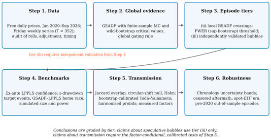
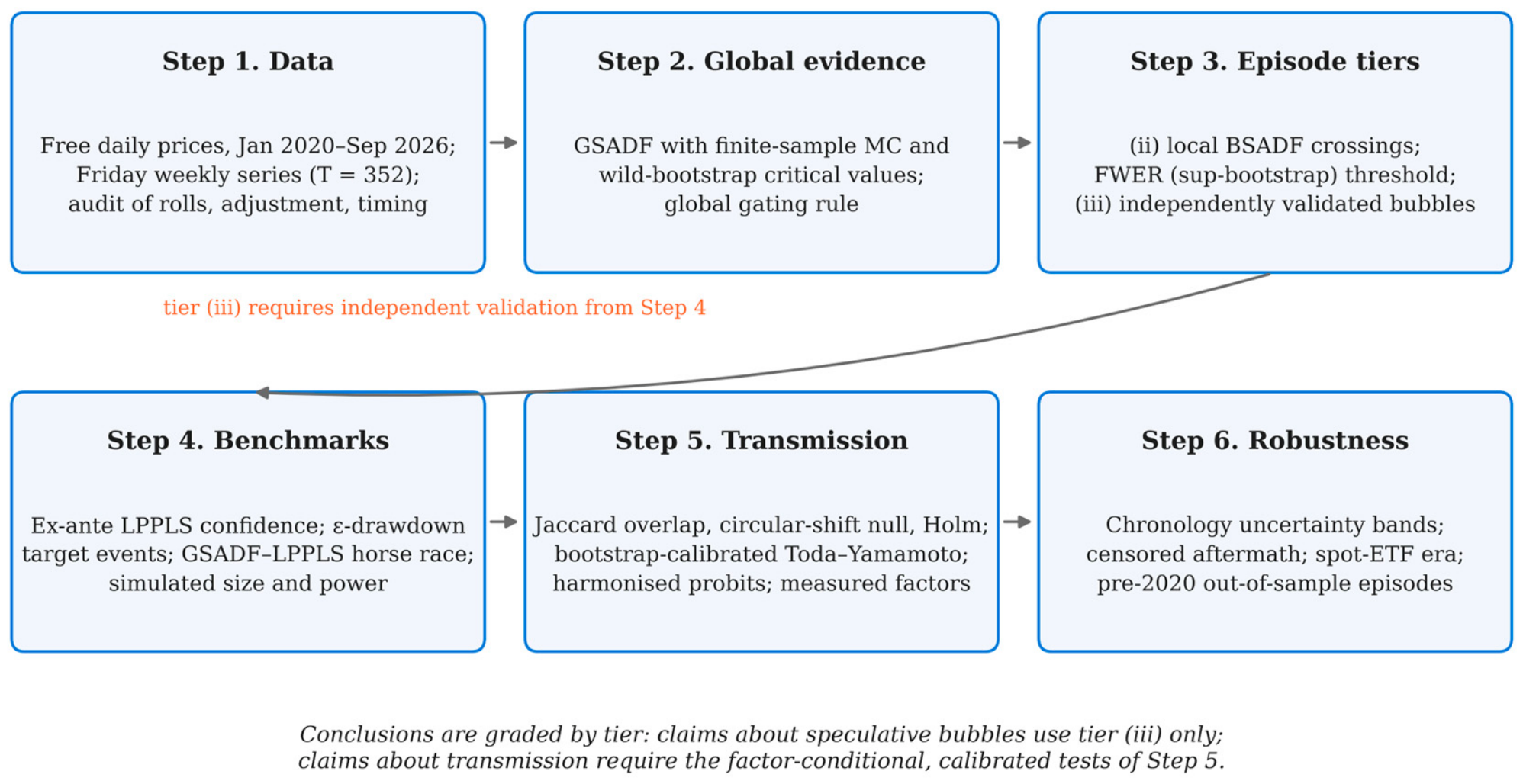
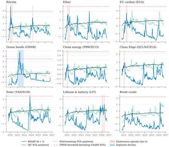
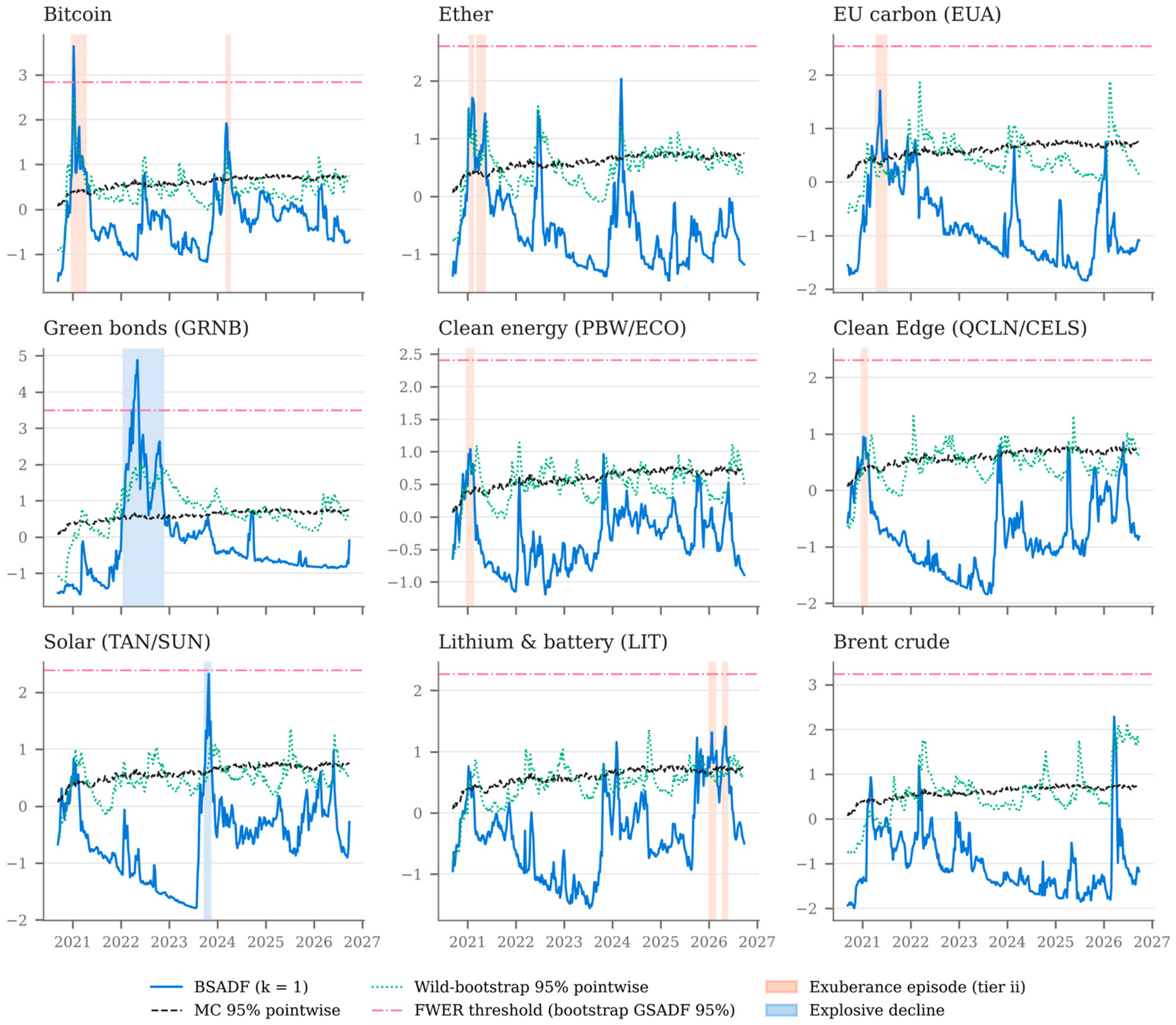
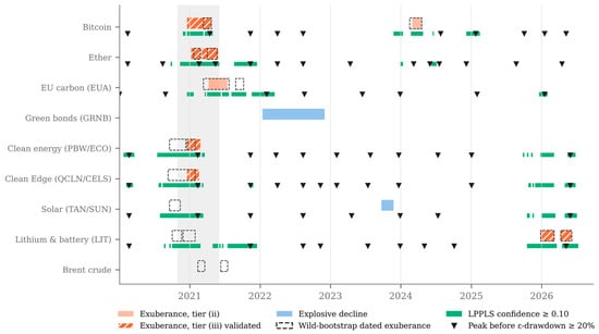
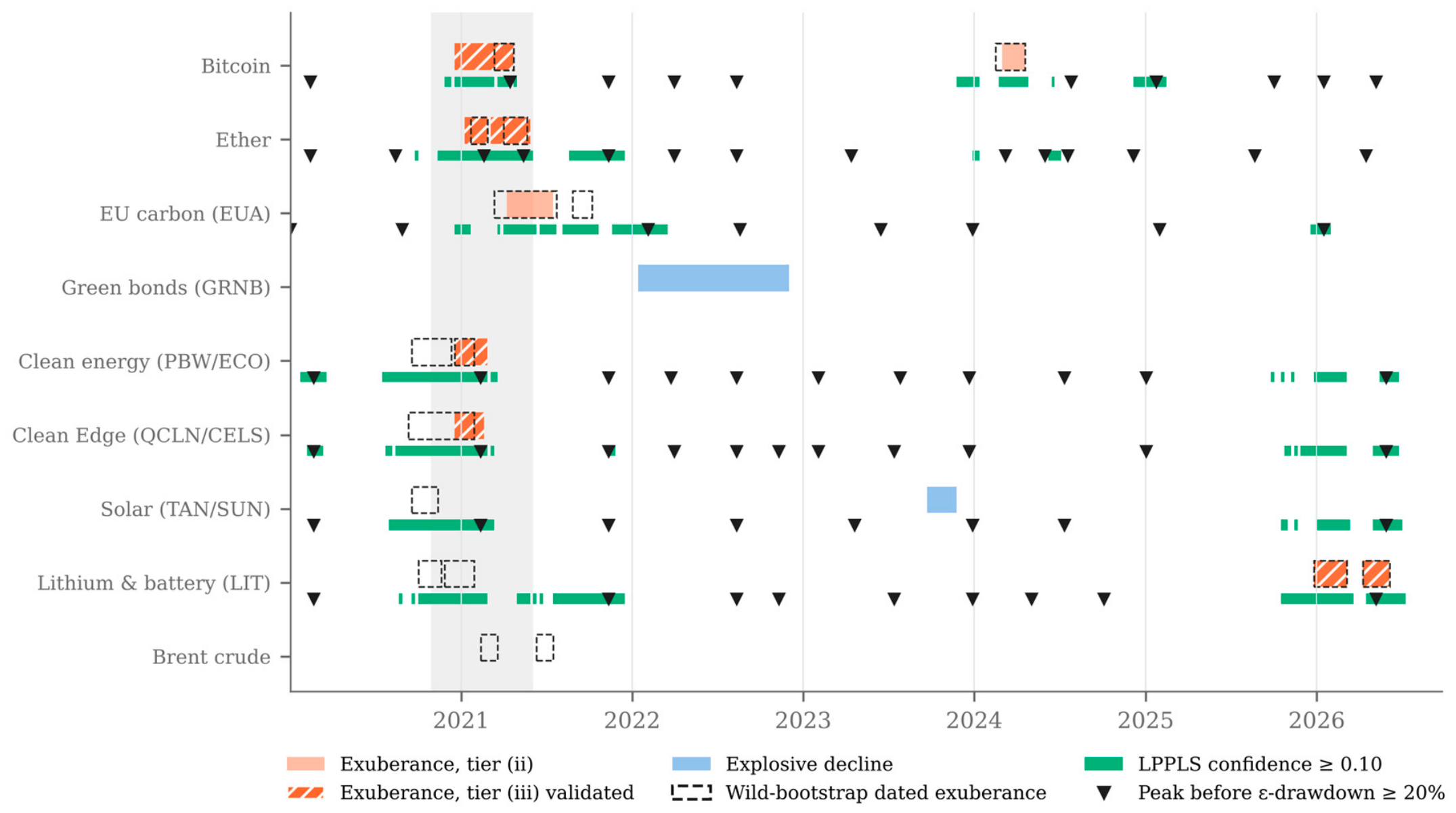
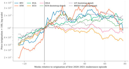
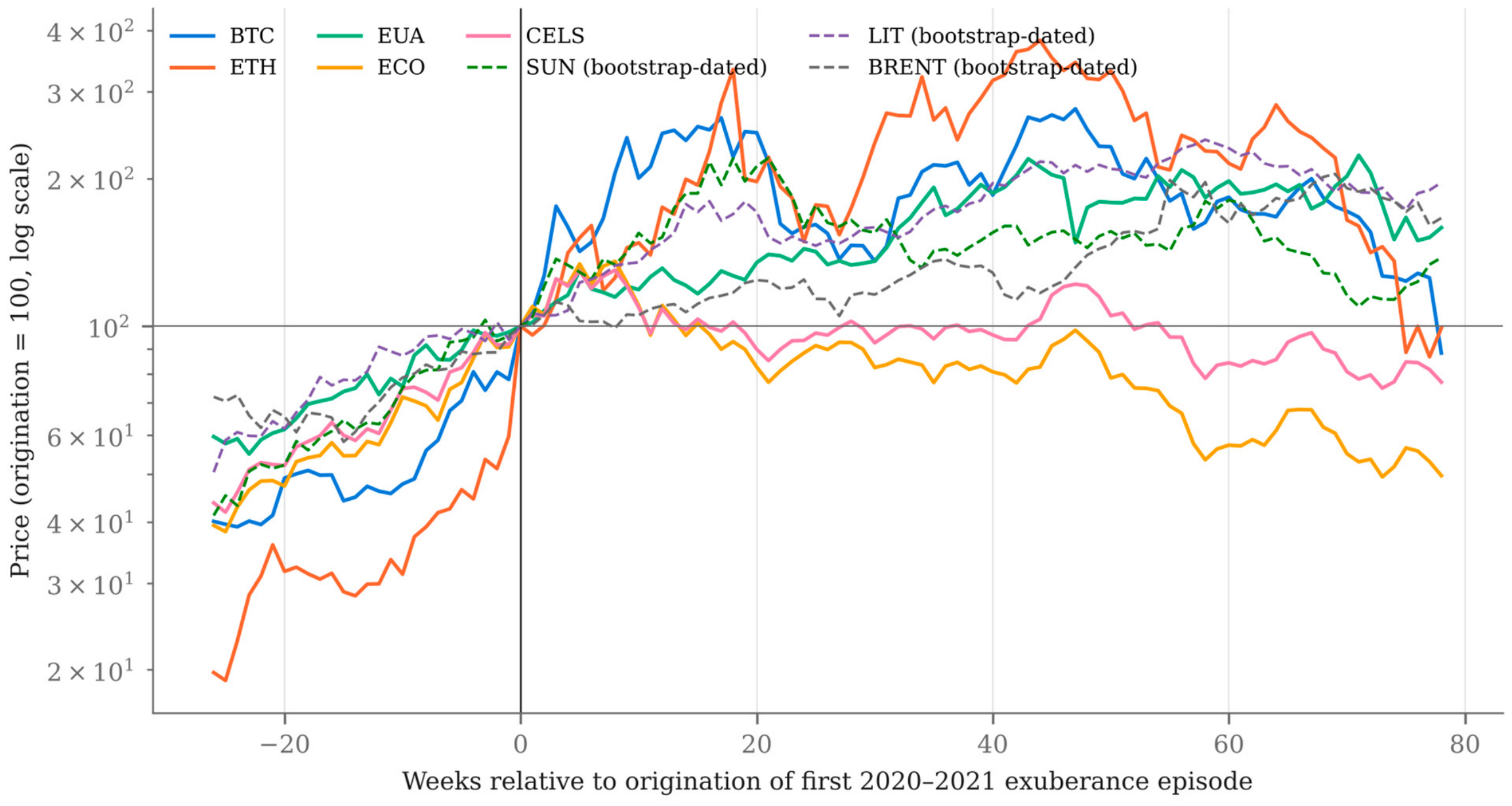

Disclaimer/Publisher’s Note: The statements, opinions and data contained in all publications are solely those of the individual author(s) and contributor(s) and not of MDPI and/or the editor(s). MDPI and/or the editor(s) disclaim responsibility for any injury to people or property resulting from any ideas, methods, instructions or products referred to in the content. |
© 2026 by the authors. Licensee MDPI, Basel, Switzerland. This article is an open access article distributed under the terms and conditions of the Creative Commons Attribution (CC BY) license.