Process-Resolved Attribution of Model-Choice Effects in Compressible Moving-Domain Flow: A Gas-Driven Launch System Study

Abstract

In compressible moving-domain computations, similar terminal responses can mask energy-input and pressure-transport biases from different origins, preventing physical attribution of modeling differences. A process-resolved model-choice attribution (PMCA) framework is therefore constructed and applied to 28 controlled cases of a 45 mm combustion light gas gun. Flow closure and heat-source normalization volume are varied independently within a shared forward problem. Differences are tracked from energy input through pressure transport and base-pressure work to the ballistic endpoint, and their stability across heat-release amounts and projectile masses is tested. The laminar closure leaves the applied energy unchanged; the first difference arises in pressure transport. Base-pressure work increases by 9.37–10.84%, mainly because temporal coupling between the pressure history and projectile motion is enhanced, rather than because the overall pressure level rises. Fixed-volume normalization first changes energy input: the applied energy exceeds the prescribed value by 3.48–10.81%, controlled by gas-region expansion during heat release. Base-pressure work then increases by 2.49–6.90%, and the two biases are approximately proportional across common conditions. Cross-condition reconstruction shows that the applied energy, pressure histories, and base-pressure work reproduce these differences in held-out conditions, whereas local peak pressures do not exhibit comparable stability. Terminal responses of strongly coupled moving domains are therefore many-to-one mappings of distinct internal transfer processes; terminal agreement does not guarantee agreement in energy input or pressure transport. PMCA advances model comparison for moving-boundary flows with volumetric sources from terminal matching to physical-process consistency checks.

1. Introduction

The combustion light gas gun (CLGG), a high-energy aerospace launch concept, propels projectiles with low-molecular-weight, high-sound-speed gas produced by hydrogen–oxygen combustion, offering a high-energy launch approach distinct from conventional solid-propellant systems [1,2]. At the same temperature, the light gas has a much higher sound speed than solid-propellant gas and therefore has the potential to overcome the driving-gas speed limit of conventional guns; Kruczynski et al. [1] provided an experimental demonstration and benchmark data for a 45 mm caliber facility. In this type of device, megajoule-level chemical energy is released within a few milliseconds, the gas pressure rises to hundreds of megapascals, and the projectile is already moving at high speed before combustion and pressure propagation are complete. The interior-ballistics process can be divided into three interrelated physical problems: the conversion of combustion heat release into gas energy, the generation and propagation of pressure in the confined gas domain, and the coupling between the projectile moving boundary and the gas flow. These three do not occur sequentially but feed back on one another over comparable timescales: rapid combustion builds up high pressure, the high pressure accelerates the projectile, projectile motion expands the gas domain and changes the density distribution and pressure-propagation path, and the modified gas domain in turn affects energy deposition and pressure evolution, forming a closed-loop coupling.

Combustion and energy release in such devices have been widely studied [2,3,4,5,6,7], spanning detailed chemical kinetics, ignition conditions, propellant composition, chamber configuration, and the deflagration-to-detonation transition. Pressure buildup and its ballistic effects have been described through interior-ballistics computational fluid dynamics (CFD) with turbulence closures and dynamic-mesh computations [8,9,10,11,12,13]; at the higher-fidelity end, the low-dissipative, structure-preserving ROUND convection schemes [14,15] have been demonstrated in implicit large-eddy simulation of compressible reacting flows [16]. The moving gas domain is computed with the arbitrary Lagrangian–Eulerian (ALE) method, the geometric conservation law, and fluid–object interaction methods [17,18,19,20,21,22,23]. These works can already connect combustion, pressure, and projectile motion, but model evaluation still relies mainly on agreement of peak pressure and muzzle velocity with experimental results.

However, peak pressure and muzzle velocity are integrated responses following the joint action of energy deposition, pressure transport, and boundary work; different internal processes can produce similar endpoints, and the terminal quantities therefore cannot determine whether an observed model difference originates from energy input or pressure transport. In more general computational fluid dynamics, Xiao et al. examined the influence of Reynolds-averaged Navier–Stokes (RANS) model-form variations on flow responses through physically constrained controlled perturbations [24]; Oberkampf and Trucano distinguished numerical error, input uncertainty, and model-form error within a verification and validation framework [25]; and Peherstorfer et al. systematically surveyed methods that exploit difference relations between models of different fidelities for cross-parameter response reconstruction [26]. These studies provide the foundations of controlled perturbation, error-source distinction, and cross-parameter difference reconstruction, respectively. Still, the three classes of methods have not yet been combined in a shared forward problem to represent discrete model forms as independently comparable variables and to locate the onset and transfer of differences along physical processes. For CLGG interior ballistics, this absence causes energy-input and pressure-transport biases to lose their source identity once they merge into projectile-base work, and makes terminal agreement unusable for judging whether internal models are equivalent.

This paper combines controlled comparison, physical-process attribution, and cross-condition difference tests into a process-resolved model-choice attribution (PMCA) framework. In a shared forward problem, the framework isolates the flow closure and the heat-source normalization volume, determines the physical process in which the two differences first appear and the way they transfer to moving-boundary work and the ballistic endpoint, and tests whether the resulting attribution is preserved as the heat-release amount and projectile mass vary.

2. Materials and Methods

2.1. Computational Model, Properties, and Numerical Settings

To compare different modeling choices on a fixed baseline, an interior-ballistics computational mapping consisting of the governing equations, property closures, and geometric constraints is established [27]. The process is described by the arbitrary Lagrangian–Eulerian (ALE) integral form of the two-dimensional axisymmetric compressible unsteady conservation equations. In the cylindrical coordinate system $(x,r)$, the computational domain $\Omega \left(t\right)$ varies with the motion of the projectile base:

$${\displaystyle \frac{\mathrm{d}}{\mathrm{d}t}}{\int }_{\Omega \left(t\right)}\mathbf{U}\mathrm{d}V+{\int }_{\partial \Omega \left(t\right)}\left({\mathbf{F}}_c-\mathbf{U}\otimes {\mathbf{v}}_g-{\mathbf{F}}_v\right)·\mathbf{n}\mathrm{d}A={\int }_{\Omega \left(t\right)}\left({\mathbf{S}}_{\mathrm{axi}}+{\mathbf{S}}_Q\right)\mathrm{d}V.$$

(1)

Here, ${\mathbf{v}}_g$ is the mesh velocity and ${\mathbf{S}}_{\mathrm{axi}}$ is the axisymmetric geometric source term. The conserved variables and the total energy per unit mass are

$$\mathbf{U}={\left[\rho ,\rho u_x,\rho u_r,\rho E_t\right]}^{\mathrm{T}},E_t=e+{\displaystyle \frac{1}{2}}\left(u_x^2+u_r^2\right).$$

(2)

The heat-release source in Equation (1) enters only the total energy equation:

$${\mathbf{S}}_Q={\left[0,0,0,{\dot{q}}^{‴}(\mathit{x},t;Q)\right]}^{\mathrm{T}}.$$

(3)

The construction of the volumetric energy source term ${\dot{q}}^{‴}$ is given in Section 2.2.

Cases A and C are closed by the RNG k–$\epsilon$ RANS model [28], whose transport equations for the turbulent kinetic energy k and its dissipation rate $\epsilon$ are

$${\displaystyle \frac{\partial \left(\rho k\right)}{\partial t}}+\nabla ·\left(\rho k\mathit{u}\right)=\nabla ·\left({\alpha }_k{\mu }_{\mathrm{eff}}\nabla k\right)+G_k-\rho \epsilon ,$$

(4)

$${\displaystyle \frac{\partial \left(\rho \epsilon \right)}{\partial t}}+\nabla ·\left(\rho \epsilon \mathit{u}\right)=\nabla ·\left({\alpha }_{\epsilon }{\mu }_{\mathrm{eff}}\nabla \epsilon \right)+C_{1\epsilon }{\displaystyle \frac{\epsilon }{k}}{G}_k-C_{2\epsilon }\rho {\displaystyle \frac{{\epsilon }^2}{k}}-R_{\epsilon },$$

(5)

where $\mathit{u}={(u_x,u_r)}^{\mathrm{T}}$ is the velocity vector, $G_k$ is the production of turbulent kinetic energy by the mean strain rate, $R_{\epsilon }$ is the RNG correction term [28], and the effective viscosity is

$${\mu }_{\mathrm{eff}}=\mu +{\mu }_t,{\mu }_t=\rho C_{\mu }{\displaystyle \frac{k^2}{\epsilon }},$$

(6)

with $C_{\mu }=0.0845$, ${\alpha }_k={\alpha }_{\epsilon }=1.393$, $C_{1\epsilon }=1.42$, and $C_{2\epsilon }=1.68$. In the laminar-control case (Case B), the modeled turbulent-viscosity contribution is removed, and molecular viscosity only is retained; all other governing equations, source terms, mesh-motion treatment, and solver settings are unchanged.

The gas composition is taken as $8{\mathrm{H}}_2+{\mathrm{O}}_2+2\mathrm{He}$. The mixture’s molar mass and specific gas constant satisfy

$$M={\displaystyle \frac{8M_{{\mathrm{H}}_2}+M_{{\mathrm{O}}_2}+2M_{\mathrm{He}}}{11}},R={\displaystyle \frac{R_u}{M}}.$$

(7)

Pressure, density, and temperature are closed by the Abel–Noble equation of state:

$$p\left({\displaystyle \frac{1}{\rho }}-b\right)=RT.$$

(8)

The mixture mass-specific constant-pressure heat capacity is synthesized from the molar constant-pressure heat capacities of the components; the molecular viscosity follows a power-law temperature dependence; the thermal conductivity is determined from a fixed Prandtl number; and the sensible enthalpy, specific enthalpy, and specific internal energy are integrated from the reference state. These property parameters are listed in Table 1.

Table 1. Gas-mixture properties and reference constants.

Parameter	Symbol	Value
Mixture molar mass	M	$5.102837\mathrm{kg}{\mathrm{kmol}}^{-1}$
Specific gas constant	R	$1629.38\mathrm{J}{\mathrm{kg}}^{-1}{\mathrm{K}}^{-1}$
Covolume	b	$1.582904027\times {10}^{-3}{\mathrm{m}}^3{\mathrm{kg}}^{-1}$
Reference temperature	$T_{\mathrm{ref}}$	$298.15\mathrm{K}$
Reference pressure	$p_{\mathrm{ref}}$	$\mathrm{101,325}\mathrm{Pa}$
Dynamic viscosity at $300\mathrm{K}$	${\mu }_{300}$	$1.30\times {10}^{-5}\mathrm{Pa}\mathrm{s}$
Viscosity temperature exponent	$n_{\mu }$	$0.70$
Prandtl number	Pr	$0.72$

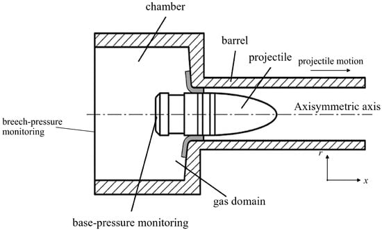
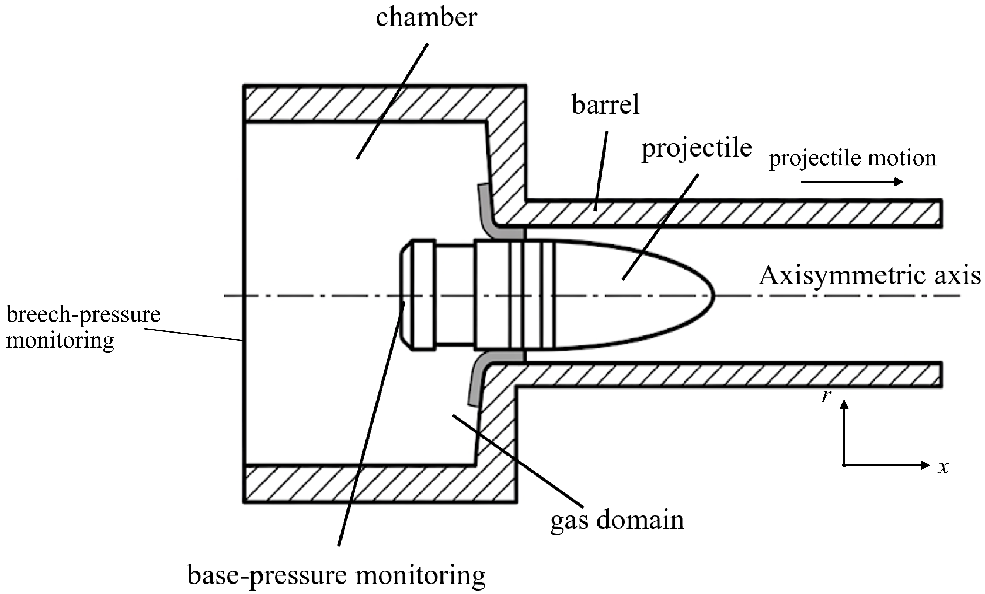
The 45 mm combustion light gas gun experimental facility reported by Kruczynski et al. [1] is used as the physical prototype, and a two-dimensional axisymmetric computational model is built based on its published geometry and operating parameters. The combustion chamber is a constant-section cylinder of volume $V_0$; its cross-sectional area equals the projectile-base area $A_b$; and the chamber length is $L_{\mathrm{ch}}=V_0/A_b$. A constant-diameter barrel of length $L_b$ is connected downstream of the chamber. Initially, the gas is uniform and at rest, and the projectile is located at the junction between the chamber and the barrel. The geometry and reference initial parameters are listed in Table 2.

Table 2. Computational-domain geometry and reference operating parameters.

Parameter	Symbol	Value
Caliber	D	$45\mathrm{mm}$
Initial gas volume	$V_0$	$5.0\times {10}^{-3}{\mathrm{m}}^3$
Barrel length	$L_b$	$4.5\mathrm{m}$
Initial temperature	$T_0$	$298\mathrm{K}$
Reference initial pressure	$p_0\left(Q_0\right)$	$38.0\mathrm{MPa}$
Total chemical energy	$Q_0$	$3.0\mathrm{MJ}$
Reference projectile mass	$m_{p,0}$	$0.520\mathrm{kg}$
Shot-start pressure	$p_r$	$172.4\mathrm{MPa}$

The values of D, $V_0$, $L_b$, $Q_0$, and $m_{p,0}$ in the table are taken from the experimental facility and conditions of Kruczynski et al. [1]. At the same time, $T_0$, $p_0\left(Q_0\right)$, and $p_r$ adopt the initial parameters listed by Liu et al. [10].

The chamber and barrel walls are adiabatic and no-slip, the breech end is fixed, the centerline is an axisymmetric boundary, and the projectile base is an axially moving wall. The breech pressure and the base pressure are taken as area averages over the corresponding surfaces:

$$p_{\mathrm{br}}\left(t\right)={\displaystyle \frac{1}{A_{\mathrm{br}}}}{\int }_{A_{\mathrm{br}}}p\mathrm{d}A,p_b\left(t\right)={\displaystyle \frac{1}{A_b}}{\int }_{A_b}p\mathrm{d}A.$$

(9)

The instant at which the base pressure first reaches $p_r$ is denoted $t_r$. For $t<t_r$ the projectile is stationary; after release, the projectile state is advanced once per physical time step in the following order:

$$\begin{array}{cc}\hfill F_p^n& =A_b{p}_b^n,\hfill \\ \hfill v_p^{n+1}& =v_p^n+{\displaystyle \frac{F_p^n}{m_p}}\Delta t,\hfill \\ \hfill s_p^{n+1}& =s_p^n+v_p^{n+1}\Delta t,\hfill \\ \hfill {\mathit{x}}_{\mathrm{mesh}}^{n+1}& =\mathcal{M}\left(s_p^{n+1}\right),\hfill \\ \hfill V_g^{n+1}& ={\int }_{{\Omega }^{n+1}}{\chi }_g(\mathit{x},t)\mathrm{d}V.\hfill \end{array}$$

(10)

with $s_p\left(t_r\right)=v_p\left(t_r\right)=0$. Here, $p_b^n$ is the area-averaged base pressure obtained from the PISO-coupled flow solution at step n, and $\mathcal{M}$ denotes the Laplace-smoothing dynamic-mesh update; the updated projectile position and mesh then define the gas region of step $n+1$. No prescribed trajectory or trajectory correction is imposed on the projectile motion. The pressure work is

$$W_p\left(t\right)={\int }_{t_r}^t{A}_b{p}_b\left(\tau \right)v_p\left(\tau \right)\mathrm{d}\tau ={\displaystyle \frac{1}{2}}{m}_p{v}_p^2\left(t\right).$$

(11)

When the axial distance between the projectile base and the muzzle is $\delta =1\mathrm{mm}$, the action time is denoted $t_{\delta }$. Linear interpolation on both sides of the terminal instant gives $v_{\delta }$ and $a_{\delta }=A_b{p}_b\left(t_{\delta }\right)/m_p$, and the muzzle velocity is taken as

$$v_{\mathrm{muzzle}}={\left(v_{\delta }^2+2a_{\delta }\delta \right)}^{1/2}.$$

(12)

The computational domain is illustrated in Figure 1.

Figure 1. Schematic of the two-dimensional axisymmetric interior-ballistic computational domain.

The governing equations are discretized by the finite-volume method [29], and the pressure–velocity coupling is treated by the PISO algorithm [30]. The numerical discretization and solver settings are listed in Table 3.

Table 3. Numerical discretization and solver-control parameters.

Item	Setting
Solver	ANSYS Fluent 2026 R1 (2D, double precision)
Baseline mesh	24,000 cells
Pressure–velocity coupling	PISO
Pressure interpolation	second-order scheme
Density, momentum, and energy	second-order upwind schemes
Turbulence transport (k and $\epsilon$)	first-order upwind schemes
Time discretization	first-order implicit scheme
Physical time step	1 $\mathsf{\mu }$s
Maximum iterations per step	50
Residual criterion	Scaled absolute residuals; continuity, x-velocity, y-velocity, k, and $\epsilon$: ${10}^{-3}$; energy: ${10}^{-6}$
Convergence checking	Enabled for all equations listed above
Dynamic mesh	Laplace smoothing

2.2. Prescribed Heat Release and the Dynamic-Volume Source Term

If the energy-input rules differ across cases, differences in responses cannot be attributed to the modeling choices themselves. All cases, therefore, adopt the same prescribed heat-release rate, and the source-intensity distortion caused by projectile motion is eliminated through dynamic-volume normalization.

The prescribed heat-release rate at the reference condition is written as

$${\dot{Q}}_0\left(t\right)=Q_{0}g\left(t\right),g\left(t\right)\ge 0,{\int }_0^{\infty }g\left(t\right)\mathrm{d}t=1.$$

(13)

The timescale of the baseline heat-release history $g\left(t\right)$ is determined with reference to the experimental pressure response in Figure 9 of Appendix B of the UTRON report [1]; the nonzero interval is $0.722$–$5.780\mathrm{ms}$, and the peak occurs at $3.330\mathrm{ms}$.

The total chemical energy of each condition is Q, and the initial gas mass is scaled proportionally at constant chemical energy per unit mass:

$$m_g\left(Q\right)={\displaystyle \frac{Q}{Q_0}}{m}_{g,0}.$$

(14)

From the Abel–Noble equation of state, the corresponding initial pressure satisfies

$$p_0\left(Q\right)={\displaystyle \frac{[m_g\left(Q\right)/V_0]R{T}_0}{1-b{m}_g\left(Q\right)/V_0}}.$$

(15)

With ${\chi }_g(\mathit{x},t)$ marking the current gas region, the volumetric energy source term is normalized by the current gas volume:

$${\dot{q}}^{‴}(\mathit{x},t;Q)={\chi }_g(\mathit{x},t){\displaystyle \frac{\dot{Q}(t;Q)}{V_g\left(t\right)}},\dot{Q}(t;Q)=Qg\left(t\right).$$

(16)

Here, $V_g\left(t\right)={\int }_{\Omega \left(t\right)}{\chi }_g(\mathit{x},t)\mathrm{d}V$ is updated as the gas region expands with projectile motion. This construction satisfies ${\int }_{\Omega \left(t\right)}{\dot{q}}^{‴}\mathrm{d}V=\dot{Q}(t;Q)$, so that the prescribed heat-release power and the total chemical energy are not affected by the expansion of the gas region.

2.3. Case Design and Operating-Condition Matrix

To separate the respective effects of the solver-closure branch and the heat-source normalization volume, the two are arranged as independent variables in a comparison matrix, following the controlled-comparison idea of computer-experiment design [31].

The operating condition is denoted $\xi =(Q,m_p)$, where Q takes $2.4$, $2.7$, $3.0$, and $3.3\mathrm{MJ}$ and $m_p$ takes $0.416$, $0.468$, $0.520$, and $0.572\mathrm{kg}$, covering the parameter range published in the UTRON report. The reference condition ${\xi }_0=(3.0\mathrm{MJ},0.520\mathrm{kg})$ corresponds to the UTRON experimental condition [1].

Case A covers all combinations of the above Q and $m_p$ values; Case B takes $(2.4,0.416)$, $(2.4,0.520)$, $(2.7,0.468)$, $(3.0,0.416)$, $(3.0,0.520)$, $(3.0,0.572)$, $(3.3,0.520)$, and $(3.3,0.572)$; Case C takes $(2.4,0.416)$, $(2.4,0.572)$, $(3.3,0.416)$, and $(3.3,0.572)$, where the parentheses list $Q/\mathrm{MJ}$ and $m_p/\mathrm{kg}$ in order.

To make the effect of each modeling setting individually identifiable, three classes of cases are defined: A is the dynamic-volume baseline case, using the RNG k–$\epsilon$ RANS [28] with normalization by the current gas volume; B is the laminar-control case, changing only the solver closure to molecular-viscosity laminar flow; C is the fixed-volume-control case, changing only the heat-source normalization volume to the initial volume $V_0$. The modeling settings of the three case classes are listed in Table 4.

Table 4. Modeling settings of the three case classes.

Case	Flow Closure	Source Normalization
A	RNG k–$\epsilon$ RANS; standard wall functions	$V_g\left(t\right)$
B	Laminar flow; molecular viscosity only	$V_g\left(t\right)$
C	RNG k–$\epsilon$ RANS; standard wall functions	$V_0$

All cases use the governing equations, gas properties, boundary conditions, and numerical settings described in Section 2.1, and the volumetric energy source is constructed as in Section 2.2. A paired comparison at the same condition changes only one modeling setting: A–B identifies the solver-closure difference, and A–C identifies the heat-source normalization-volume difference.

2.4. Physical-Transport-Stage Response Measures and the Cross-Condition Stability Test

To locate the transport stage at which a modeling difference first appears and to test the stability of this conclusion over the condition domain, response measures for the physical transport stages and a cross-condition stability criterion are established.

The conservation-law connection among the stages is first established from the ALE energy equation. The applied power at the energy-input stage is obtained by integrating the volumetric energy source over the gas region:

$${\dot{Q}}_{\mathrm{app}}\left(t\right)={\int }_{\Omega \left(t\right)}{\dot{q}}^{‴}(\mathit{x},t;Q)\mathrm{d}V,Q_{\mathrm{app}}\left(t\right)={\int }_0^t{\dot{Q}}_{\mathrm{app}}\left(\tau \right)\mathrm{d}\tau .$$

(17)

Under the pressure-driven base relation of Equation (10), the energy equation is integrated over the gas domain $\Omega \left(t\right)$ moving with the projectile base. The adiabatic fixed walls contribute no energy flux, and the moving base contributes the boundary power $A_b{p}_b\left(t\right)v_p\left(t\right)$, so that

$${\displaystyle \frac{\mathrm{d}}{\mathrm{d}t}}{\int }_{\Omega \left(t\right)}\rho E_t\mathrm{d}V={\dot{Q}}_{\mathrm{app}}\left(t\right)-A_b{p}_b\left(t\right)v_p\left(t\right).$$

(18)

Integrating from 0 to $t_{\delta }$ and combining with Equation (11) yields the overall energy constraint

$$Q_{\mathrm{app}}\left(t_{\delta }\right)=\Delta E_t+W_p\left(t_{\delta }\right),\Delta E_t={\int }_{\Omega \left(t_{\delta }\right)}\rho E_t\mathrm{d}V-{\int }_{\Omega \left(0\right)}\rho E_t\mathrm{d}V.$$

(19)

The pressure-transport stage is characterized by the breech pressure $p_{\mathrm{br}}\left(t\right)$, the base pressure $p_b\left(t\right)$, and their difference $\Delta p\left(t\right)=p_{\mathrm{br}}\left(t\right)-p_b\left(t\right)$; the base-work stage is characterized by the pressure work $W_p\left(t_{\delta }\right)$ at the terminal instant; and the ballistic-response stage by the action time $t_{\delta }$ and the muzzle velocity $v_{\mathrm{muzzle}}$. The four physical transport stages form the $E\to F\to W\to B$ transport chain; a stage-by-stage comparison along this chain determines the transport stage at which a modeling-setting difference first appears.

The response difference of case j relative to case A is defined as follows:

$${\Delta }_{j}Y\left(\xi \right)=Y(\xi ,j)-Y(\xi ,\mathrm{A}),j\in \{\mathrm{B},\mathrm{C}\}.$$

(20)

History responses are compared over the interior-ballistics interval $I_j=[0,\min (t_{\delta ,\mathrm{A}},t_{\delta ,j})]$ common to both cases, with the dimensionless differences:

$$\begin{array}{cc}\hfill d_t(f_j,f_{\mathrm{A}})& ={\left[{\displaystyle \frac{{\displaystyle {\int }_{I_j}{(f_j-f_{\mathrm{A}})}^2\mathrm{d}t}}{{\displaystyle {\int }_{I_j}{f}_{\mathrm{A}}^2\mathrm{d}t}}}\right]}^{1/2},\hfill \\ \hfill d_s(Y_j,Y_{\mathrm{A}})& ={\displaystyle \frac{|Y_j-Y_{\mathrm{A}}|}{|Y_{\mathrm{A}}|}}.\hfill \end{array}$$

(21)

Here, $d_t$ is the relative $L^2$ perturbation norm on the baseline response.

The comparison above locates the physical transport stage where the difference first appears at the reference condition, but it is insufficient to judge the stability of this stage relation over the condition domain. For this purpose, the case response difference is expanded locally in a Taylor series about ${\xi }_0$. With ${\eta }_Q=(Q-Q_0)/Q_0$ and ${\eta }_m=(m_p-m_{p,0})/m_{p,0}$:

$${\Delta }_{j}Y\left(\xi \right)={\Delta }_{j}Y\left({\xi }_0\right)+{\left.{\displaystyle \frac{\partial {\Delta }_{j}Y}{\partial {\eta }_Q}}\right|}_{{\xi }_0}{\eta }_Q+{\left.{\displaystyle \frac{\partial {\Delta }_{j}Y}{\partial {\eta }_m}}\right|}_{{\xi }_0}{\eta }_m+{\mathcal{O}(\parallel \eta \parallel }^2).$$

(22)

The coefficients are denoted ${\beta }_0$, ${\beta }_Q$, and ${\beta }_m$, and are estimated from the condition data as ${\widehat{\beta }}_0$, ${\widehat{\beta }}_Q$, and ${\widehat{\beta }}_m$; retaining the first-order terms gives

$$\widehat{{\Delta }_{j}Y}\left(\xi \right)={\widehat{\beta }}_0+{\widehat{\beta }}_Q{\eta }_Q+{\widehat{\beta }}_m{\eta }_m.$$

(23)

After the i-th condition is left out, the coefficients of Equation (23) are re-estimated from the remaining conditions, giving the difference prediction ${\widehat{{\Delta }_{j}Y}}^{(-i)}$; the case-A response is then reconstructed from the case-j response at the held-out condition:

$${\widehat{Y}}_{\mathrm{A},i}^{(-i)}=Y({\xi }_i,j)-{\widehat{{\Delta }_{j}Y}}^{(-i)}\left({\xi }_i\right).$$

(24)

The reduction of the leave-one-out reconstruction error relative to the raw case difference is

$$G_{j,Y}=1-{\displaystyle \frac{{\epsilon }_{\mathrm{LOO}}}{{\epsilon }_{\mathrm{raw}}}}.$$

(25)

The criterion $G_{j,Y}>0$ is taken to indicate that the case-difference relation is stable across conditions. In what follows, the A–B and A–C pairs are referred to as the laminar-control pair and the fixed-volume-control pair, respectively.

3. Results

3.1. Reference-Condition Verification and the Baseline Case

Case A serves as the baseline for the subsequent same-condition pairs; its ballistic endpoint responses are compared with published results in Table 5. The reference condition is ${\xi }_0=(3.0\mathrm{MJ}, 0.520\mathrm{kg})$.

Table 5. Ballistic responses at the reference condition compared with published results.

Response Quantity	Simulation Value	Experimental Value	Premixed-Model Computation
Muzzle velocity$/\mathrm{m}{\mathrm{s}}^{-1}$	1800.439	1700	1800
Muzzle kinetic energy$/\mathrm{MJ}$	0.842811	0.751400	0.842400
Ballistic efficiency	0.28094	0.25	0.28

The muzzle velocity computed here differs from the premixed-model computation by $0.024\%$, the muzzle kinetic energy by about $0.05\%$, and the ballistic efficiency by about $0.34\%$; relative to the experimental value, the muzzle velocity is higher by about $5.9\%$. The cumulative applied energy of the reference case is $3.000\mathrm{MJ}$; at the terminal instant, the base-pressure work and the projectile kinetic energy are $0.842820\mathrm{MJ}$ and $0.842706\mathrm{MJ}$, respectively, a relative difference of $0.0135\%$. The action time is $t_{\delta }=7.603\mathrm{ms}$.

To verify the sensitivity of the reported responses to the baseline discretization, two additional calculations of the baseline case were performed under identical physical models, source terms, and boundary conditions: one with the time step halved to $0.5\mathsf{\mu }\mathrm{s}$ and one with the mesh coarsened fourfold to 6,000 cells (Table 6).

Table 6. Discretization-sensitivity check of the baseline case at the reference condition.

		Time Step $0.5\mathsf{\mu }\mathbf{s}$		6000-Cell Mesh
Quantity	Baseline	Value	Deviation/%	Value	Deviation/%
Exit time$/\mathrm{ms}$	7.60251	7.62148	0.250	7.64425	0.549
Muzzle velocity$/\mathrm{m}{\mathrm{s}}^{-1}$	1800.33	1789.85	0.582	1767.93	1.799
Peak base pressure$/\mathrm{MPa}$	174.47	174.22	0.144	174.84	0.209
Peak breech pressure$/\mathrm{MPa}$	261.26	261.40	0.054	260.83	0.165
Base-pressure work$/\mathrm{MJ}$	0.8430	0.8330	1.190	0.8129	3.571

The key scalar responses vary by at most $0.6\%$ under time-step halving and by at most $1.8\%$ under fourfold mesh coarsening, with the local base-pressure history deviating by about $6\%$; the baseline discretization is therefore retained for all cases in this study.

3.2. Physical-Transport-Stage Responses of the Modeling Differences

To identify the transport stage at which the difference induced by each modeling choice arises, cases A, B, and C are compared at the corner condition $(Q,m_p)=(3.3\mathrm{MJ}, 0.572\mathrm{kg})$, where all three case classes are defined. The responses at each transport stage, from the cumulative applied energy to the ballistic endpoint, are listed in Table 7.

Table 7. Physical-transport-stage results of the three case classes at $(Q,m_p)=(3.3\mathrm{MJ}, 0.572\mathrm{kg})$.

Transport Stage	Response Quantity	A	B	C
E	Cumulative applied energy$/\mathrm{MJ}$	3.3000	3.3000	3.5892
F	Peak breech pressure$/\mathrm{MPa}$	279.796	279.789	286.924
F	Peak base pressure$/\mathrm{MPa}$	182.460	184.878	185.538
W	Base-pressure work$/\mathrm{MJ}$	0.9273	1.0181	0.9805
B	Action time$/\mathrm{ms}$	7.4431	7.3644	7.3492
B	Muzzle velocity$/\mathrm{m}{\mathrm{s}}^{-1}$	1800.626	1886.814	1851.583

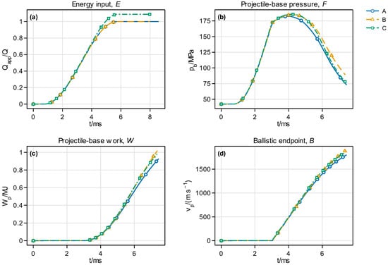
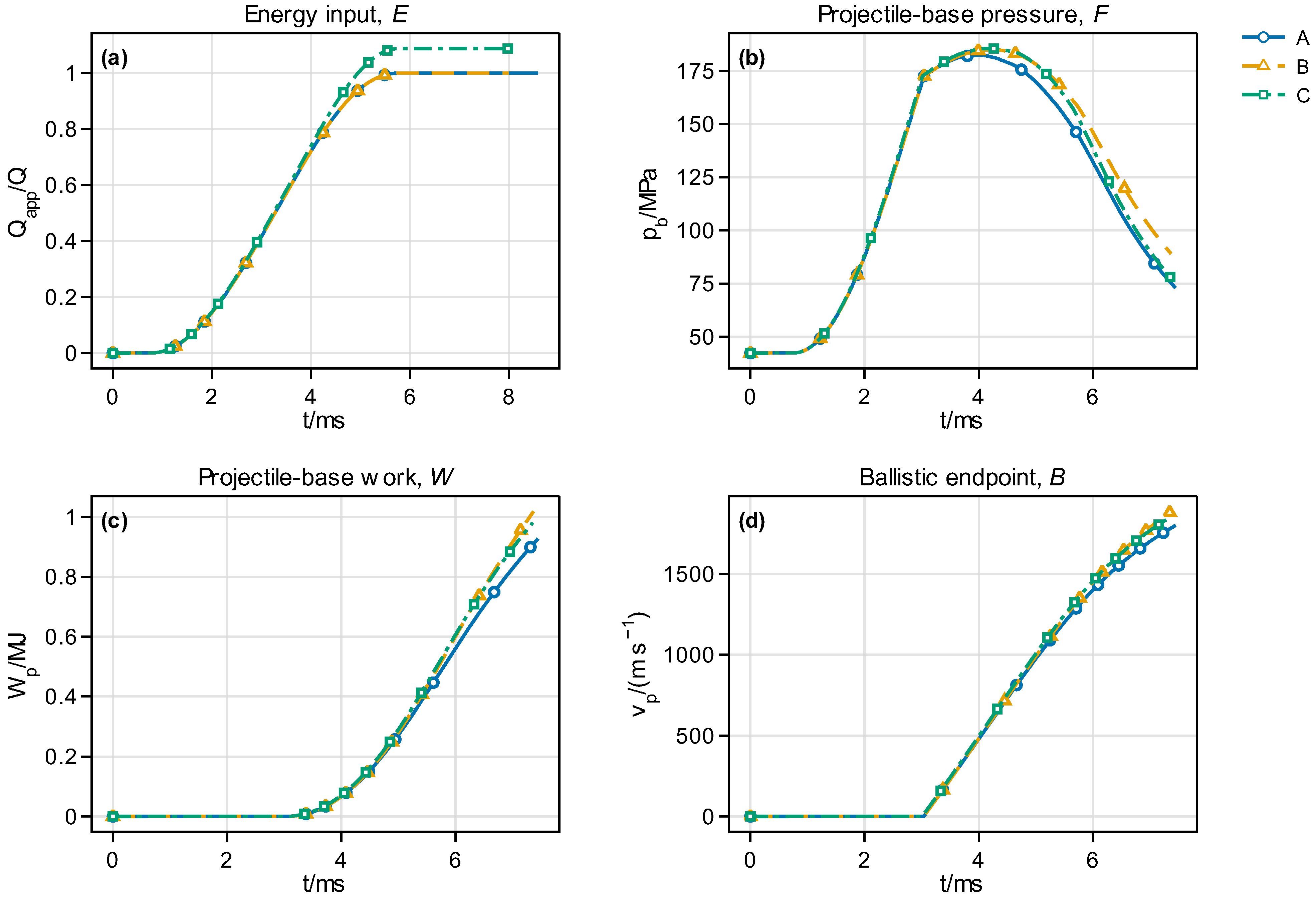
The evolution of these stage differences along the $E\to F\to W\to B$ transport chain is shown in Figure 2.

Figure 2. Physical-transport-stage responses of the three case classes at $(Q,m_p)=(3.3\mathrm{MJ}, 0.572\mathrm{kg})$: (a) cumulative applied-energy ratio $Q_{\mathrm{app}}\left(t\right)/Q$; (b) base pressure $p_b\left(t\right)$; (c) base-pressure work $W_p\left(t\right)$; (d) projectile velocity $v_p\left(t\right)$. The markers at the ends of the curves in panel (d) indicate the muzzle velocity of the corresponding case.

In the figure, the applied-energy curves of A and B coincide over the whole action time, whereas the curve of C lies above them. With identical energy input, the base-pressure histories of A and B separate, and the separation propagates through the base-pressure work to the projectile velocity; C separates from A and B already in the applied energy and maintains the offset through all subsequent responses. The first separation of the response sequences locates the closure difference at the pressure-transport stage and the normalization-volume difference at the energy-input stage.

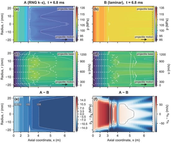
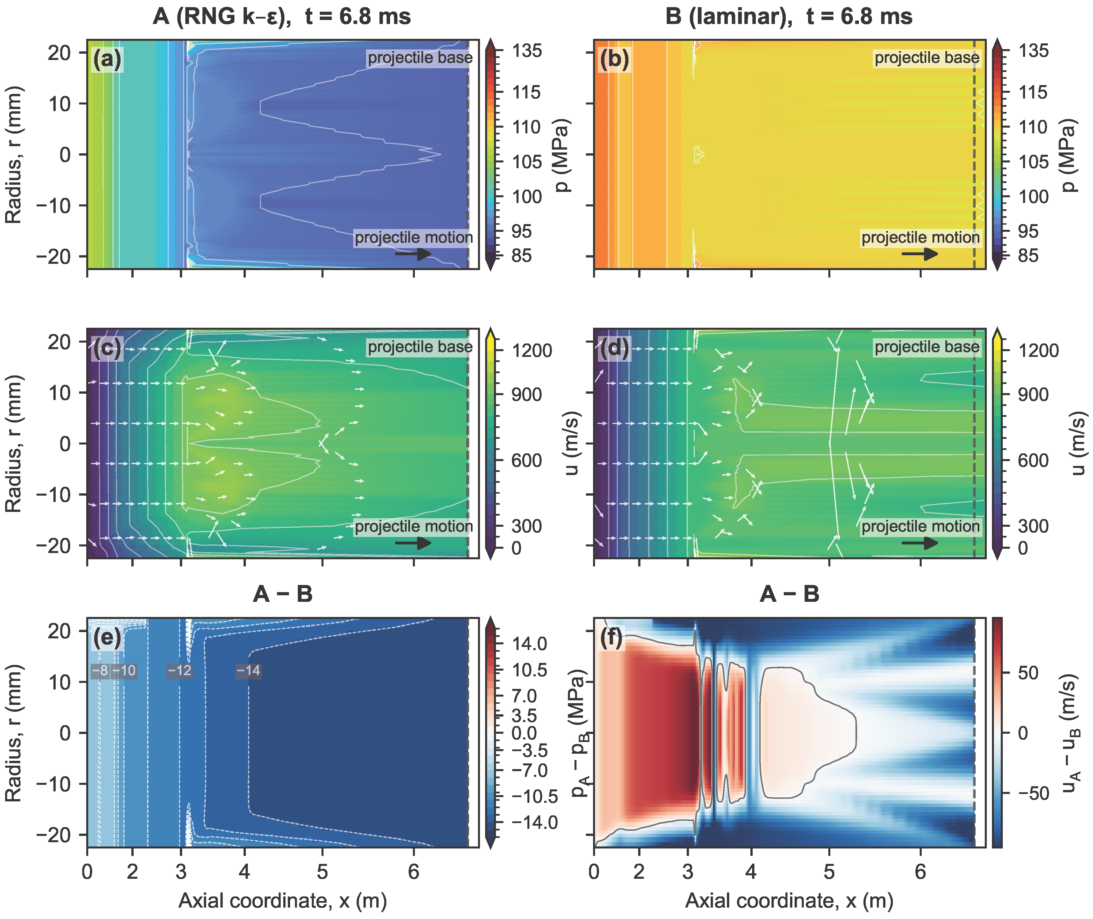
The same pair is further examined at the field level in Figure 3, which compares the instantaneous pressure and axial-velocity fields of cases A and B at $t=6.8$ ms, $0.6$ ms before muzzle exit of case A.

Figure 3. Instantaneous fields of cases A and B at $(Q,m_p)=(3.3\mathrm{MJ}, 0.572\mathrm{kg})$, $t=6.8$ ms: (a,b) pressure; (c,d) axial velocity; (e) pressure difference $p_A-p_B$; (f) axial-velocity difference $u_A-u_B$. The dashed line marks the projectile-base position of case A. The white arrows indicate streamlines of the instantaneous velocity field.

In the figure, the pressure fields of the two cases share the same overall structure, while their difference $p_A-p_B$ is negative throughout the bore and increases in magnitude along the axis: about $-8$ MPa at the breech and about $-14.5$ MPa at the projectile base. The axial-velocity difference alternates in sign along the axis and forms alternating bands. The closure difference is thus distributed over the entire pressure field between the breech and the projectile base.

3.3. Cross-Condition Stability of the Transport-Stage Differences

Section 3.2 presented the response sequences of A, B, and C at the representative condition. This section tests whether the relative relations of these response differences can be reconstructed at other $(Q,m_p)$ combinations.

The correction gain is computed by leave-one-out reconstruction:

$$G=1-{\displaystyle \frac{{\epsilon }_{\mathrm{LOO}}}{{\epsilon }_{\mathrm{raw}}}},$$

(26)

where ${\epsilon }_{\mathrm{raw}}$ is the root-mean-square error of the raw case difference, and ${\epsilon }_{\mathrm{LOO}}$ is the root-mean-square error between the reconstructed and actual case-A responses. $G>0$ indicates that the difference relation is reconstructed at the held-out condition. The results are listed in Table 8.

Table 8. Leave-one-out reconstruction gains of cases B and C.

Response Quantity	Case B	Case C
Applied energy	–	0.766
Breech-pressure history	0.829	0.835
Base-pressure history	0.951	0.831
Breech-to-base pressure-difference history	0.842	0.715
Base-pressure work	0.954	0.853
Action time	0.819	0.992
Muzzle velocity	0.959	0.708
Peak breech pressure	−0.438	0.866
Peak base pressure	0.316	−1.011

The leave-one-out results show that case B obtains positive gains for the base-pressure history, base-pressure work, action time, and muzzle velocity, and case C obtains positive gains for the applied energy, pressure histories, base-pressure work, action time, and muzzle velocity. The positive gains of these quantities at held-out conditions indicate that the response-difference relations observed at the representative condition are not confined to a single condition.

4. Discussion

4.1. Onset of the Differences Between the Two Modeling Choices

The response comparison in Section 3 shows that the offsets of B and C first appear in pressure transport and applied energy, respectively, and the leave-one-out reconstruction further demonstrates that this order of appearance is preserved across conditions. This section explains the formation mechanisms of the two differences in terms of the flow closure and moving-domain source-term conservation. The condition $(Q,m_p)=(3.3\mathrm{MJ}, 0.572\mathrm{kg})$, covered by all three case classes, is selected; with the dynamic-volume baseline A as the reference, the responses of B and C are expressed as relative offsets $\Delta X=(X-X_A)/X_A$. If the difference of B originates from viscous transport, its offset should first appear in pressure-wave propagation and the base-pressure buildup process; if the difference of C originates from source-term normalization, its offset should first appear in the applied energy. Table 9 gives the quantitative offsets of the response quantities.

Table 9. Response offsets of the two modeling choices at the representative condition.

Case	$\mathbf{\Delta }({\mathit{Q}}_{\mathbf{app}}/\mathit{Q})$ (%)	$\mathbf{\Delta }{\mathit{p}}_{\mathit{b},\max }$ (%)	$\mathbf{\Delta }{\mathit{W}}_{\mathit{p}}$ (%)	$\mathbf{\Delta }{\mathit{t}}_{\mathit{\delta }}$ (%)	$\mathbf{\Delta }{\mathit{v}}_{\mathbf{muzzle}}$ (%)
B	0.00	+1.33	+9.80	−1.06	+4.79
C	+8.76	+1.69	+5.74	−1.26	+2.83

B and A share the same prescribed heat-release history and dynamic-volume normalization, and $Q_{\mathrm{app}}/Q$ is unchanged, so an applied-energy increment cannot explain the subsequent response offsets. The two flow closures first change the viscous momentum transport and dissipation in the ALE equations: the RNG k–$\epsilon$ branch represents unresolved fluctuations through turbulent viscosity, whereas the laminar branch retains only molecular viscosity. The propagation and attenuation of pressure waves and the pressure-buildup process near the projectile base are therefore changed, and the synchronization between $p_b\left(t\right)$ and $v_p\left(t\right)$ changes accordingly. The pressure-work increment comes from the time integral of $A_b{p}_b\left(t\right)v_p\left(t\right)$ in Equation (11), not from a single-point offset of the peak pressure.

The difference between C and A first appears in the applied energy. C replaces the projectile-motion-updated $V_g\left(t\right)$ by $V_0$ in the source-term normalization; when $V_g\left(t\right)>V_0$, the fixed-volume rule amplifies the local source intensity by $V_g\left(t\right)/V_0$. The added internal energy changes the pressure history through the equation of state and is then converted into pressure work and terminal kinetic energy by the moving base. The pressure and ballistic-response offsets of C therefore inherit the volume-normalization bias at the input end.

This comparison yields two testable criteria for mechanisms. If the difference of B is produced by pressure transport, the moving-boundary-weighted pressure-transfer coefficient from the breech pressure to base work, and the degree of temporal coupling between the base pressure and the boundary velocity, should change consistently across the eight common conditions. If the difference in C is produced by source-term normalization, the applied-energy bias should equal the temporal-coupling functional of the normalized heat-release history and the gas-region expansion history. Section 4.2 and Section 4.3 test these two criteria, respectively.

4.2. Pressure-Transport and Work Responses Induced by the Laminar Closure

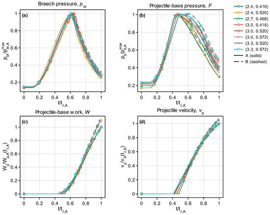
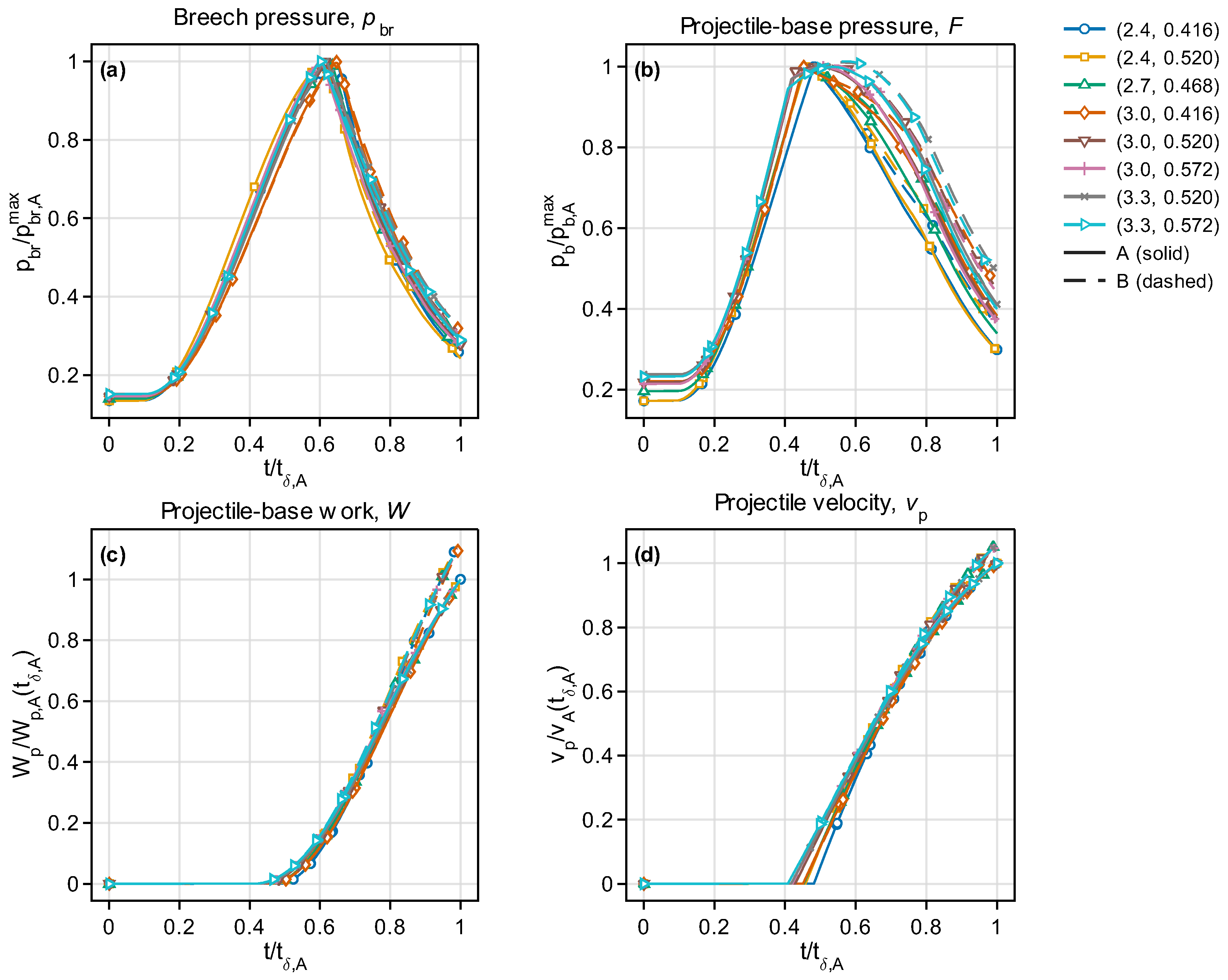
A and B share eight $(Q,m_p)$ conditions. The two case classes use the same prescribed heat-release history, dynamic-volume normalization, geometric motion, and numerical settings, changing only the solver closure. Figure 4 shows how the pressure-transport offset induced by the laminar closure accumulates into base work and ballistic responses.

Figure 4. Pressure-transport, base-work, and ballistic-response offsets induced by the laminar closure: (a) breech-pressure history; (b) projectile-base pressure history; (c) projectile-base work; (d) projectile velocity. Solid lines: case A (dynamic-volume baseline); dashed lines: case B (laminar closure); colors denote the eight operating conditions. Solid and dashed curves of the same color are close during breech-pressure buildup and separate progressively in the base-pressure, work, and velocity responses.

In the figure, the solid and dashed lines of the same color are close during the breech-pressure buildup stage and then gradually separate in the base-pressure, pressure-work, and projectile-velocity histories, indicating that the observable difference of the laminar closure enters through the pressure-transport process and accumulates toward the endpoint responses.

To distinguish the contributions of the pressure-history amplitude, the moving-boundary velocity amplitude, and their temporal synchronization to the pressure work, the time inner product and the $L^2$ norm are defined as follows:

$$⟨f,h⟩={\int }_0^{t_{\delta }}f\left(t\right)h\left(t\right)\mathrm{d}t,{\parallel f\parallel }_2={\left[{\int }_0^{t_{\delta }}{f}^2\left(t\right)\mathrm{d}t\right]}^{1/2}.$$

(27)

The temporal-coupling coefficient between the base pressure and the moving-boundary velocity is defined as follows:

$${\mathsf{\Gamma }}_{pv}={\displaystyle \frac{⟨p_b,v_p⟩}{\parallel p_b{\parallel }_2{\parallel v_p\parallel }_2}},0\le {\mathsf{\Gamma }}_{pv}\le 1.$$

(28)

From Equation (11), the pressure work admits the exact decomposition:

$$W_p=A_b\parallel p_b{\parallel }_2{\parallel v_p\parallel }_2{\mathsf{\Gamma }}_{pv},$$

(29)

With $\Delta \ln X=\ln (X_B/X_A)$, A and B satisfy the log-difference identity:

$$\Delta \ln W_p=\Delta \ln \parallel p_b{\parallel }_2+\Delta \ln {\parallel v_p\parallel }_2+\Delta \ln {\mathsf{\Gamma }}_{pv}.$$

(30)

The three additive terms $C_p=100\Delta \ln {\parallel p_b\parallel }_2$, $C_v=100\Delta \ln {\parallel v_p\parallel }_2$, and $C_c=100\Delta \ln {\mathsf{\Gamma }}_{pv}$ denote the contributions of the pressure-history amplitude, the moving-boundary velocity amplitude, and their temporal synchronization to the pressure-work offset, and they sum to $C_W=100\Delta \ln W_p$. These additive logarithmic terms differ from the ordinary relative difference ${\delta }_X=100(X_{\mathrm{B}}-X_{\mathrm{A}})/X_{\mathrm{A}}$ used elsewhere in this paper; the two families coincide only to first order.

The moving-boundary-weighted pressure-transfer coefficient is further defined as follows:

$${\eta }_{pb}={\displaystyle \frac{{\displaystyle {\int }_0^{t_{\delta }}{p}_b\left(t\right)v_p\left(t\right)\mathrm{d}t}}{{\displaystyle {\int }_0^{t_{\delta }}{p}_{\mathrm{br}}\left(t\right)v_p\left(t\right)\mathrm{d}t}}}.$$

(31)

${\eta }_{pb}$ compares the actual base-pressure work kernel with the work potential constructed from the breech pressure, characterizing the extent to which the breech pressure is retained in moving-boundary work; ${\mathsf{\Gamma }}_{pv}$ separates the degree of temporal synchronization between $p_b\left(t\right)$ and $v_p\left(t\right)$ from the pressure amplitude. Equation (30) further decomposes the pressure-work offset exactly into three contributions: pressure-history amplitude, boundary-velocity amplitude, and pressure–motion coupling. The condition-by-condition results are listed in Table 10.

Table 10. Pressure-transport measures and logarithmic decomposition of pressure-work offsets under the laminar closure.

(a) Pressure Transfer and Pressure–Motion Coupling
Condition	${\mathit{\eta }}_{\mathit{pb}}$		${\mathsf{\Gamma }}_{\mathit{pv}}$
	A	B	A	B
$(2.4,0.416)$	0.788	0.831	0.582	0.615
$(2.4,0.520)$	0.832	0.872	0.593	0.626
$(2.7,0.468)$	0.792	0.833	0.624	0.656
$(3.0,0.416)$	0.746	0.787	0.648	0.677
$(3.0,0.520)$	0.795	0.835	0.656	0.686
$(3.0,0.572)$	0.813	0.853	0.658	0.687
$(3.3,0.520)$	0.779	0.819	0.679	0.709
$(3.3,0.572)$	0.798	0.837	0.681	0.710
(b) Logarithmic Contributions to Pressure Work
Condition	${\mathit{C}}_{\mathit{p}}$ (%)	${\mathit{C}}_{\mathit{v}}$ (%)	${\mathit{C}}_{\mathit{c}}$ (%)	${\mathit{C}}_{\mathit{W}}$ (%)
$(2.4,0.416)$	2.99	1.66	5.56	10.21
$(2.4,0.520)$	3.15	1.68	5.45	10.29
$(2.7,0.468)$	3.31	1.61	5.00	9.92
$(3.0,0.416)$	3.18	1.40	4.37	8.95
$(3.0,0.520)$	3.54	1.56	4.56	9.65
$(3.0,0.572)$	3.38	1.45	4.32	9.15
$(3.3,0.520)$	3.63	1.49	4.20	9.32
$(3.3,0.572)$	3.68	1.51	4.16	9.35

Note. Here $\Delta \ln X\equiv \ln (X_{\mathrm{B}}/X_{\mathrm{A}})$ for the A–B comparison. Thus, $C_p=100\Delta \ln {\parallel p_b\parallel }_2$, $C_v=100\Delta \ln {\parallel v_p\parallel }_2$, $C_c=100\Delta \ln {\mathsf{\Gamma }}_{pv}$, and $C_W=100\Delta \ln W_p$; all four quantities are reported in percent.

A and B use the same prescribed heat-release history and dynamic-volume normalization, and Equation (16) guarantees identical volume-integrated heat input, so no energy increment is available at the input end for B to inherit. The difference between the two case classes enters only the transport closure of the ALE equations: the RNG k–$\epsilon$ branch converts unresolved fluctuations into turbulent viscosity and dissipation, whereas the laminar branch retains only molecular viscosity. The axial momentum flux driven by the pressure gradient, the attenuation of pressure waves, and the pressure-buildup rate near the projectile base are changed accordingly.

${\eta }_{pb}$ is higher for B than for A in all eight conditions, with relative increases of $4.83$–$5.49\%$; ${\mathsf{\Gamma }}_{pv}$ rises from $0.582$–$0.681$ for A to $0.615$–$0.710$ for B, with relative increases of $4.25$–$5.71\%$. The former indicates increased retention of breech pressure in moving-boundary work, and the latter indicates enhanced temporal synchronization between the base-pressure history and the projectile-velocity history. The pressure difference, therefore, contains both spatial transport and temporal coupling changes, rather than a single-point change in the local breech pressure.

In the logarithmic decomposition of the pressure work, $C_p$ accounts for $2.99$–$3.68\%$, $C_v$ for $1.40$–$1.68\%$, and $C_c$ for $4.16$–$5.56\%$ of the total logarithmic pressure-work difference; the three terms sum to $C_W$ under all conditions. The coupling term is consistently larger than the pressure-amplitude and velocity-amplitude terms, indicating that the pressure-work increase arises mainly from the enhanced synchronous integration of $p_b\left(t\right)$ and $v_p\left(t\right)$ after the pressure-transport change, rather than from an overall rise in pressure amplitude.

As the boundary driver in Equation (10), the base pressure changes its waveform, $p_b\left(t\right)$ and $v_p\left(t\right)$ adjust synchronously, and the instantaneous power $A_b{p}_b\left(t\right)v_p\left(t\right)$ is redistributed over the action time. The base-pressure work of B increases by $9.37$–$10.84\%$, the action time shortens by $0.74$–$1.14\%$, and the muzzle velocity still increases by $4.58$–$5.28\%$; the closure difference is transmitted to the endpoint through the integral effect of the pressure history rather than through a single peak. The base pressure simultaneously controls the projectile acceleration and the gas-domain boundary position; an increased velocity changes the subsequent gas volume and the pressure-wave propagation distance, forming feedback between pressure transport and the moving boundary. The physical entry of the laminar closure is thus located in the pressure-transport process, and the pressure work and muzzle velocity retain the time-integrated information of this transport difference.

The A–B comparison is conducted at the engineering fidelity level of interior-ballistics modeling: the RNG k–$\epsilon$ closure is consistent with the mesh scales used here, and the discretization sensitivity audit in Section 3.1 confirms that the reported attribution is not altered by the mesh or the time step. The higher-fidelity route noted in Section 1, LES closures combined with low-dissipative convection schemes of the ROUND type, would allow the pressure-transport onset identified above to be examined without modeled turbulent viscosity.

4.3. Energy-Input Bias Induced by Fixed-Volume Normalization

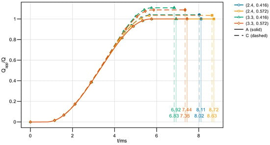
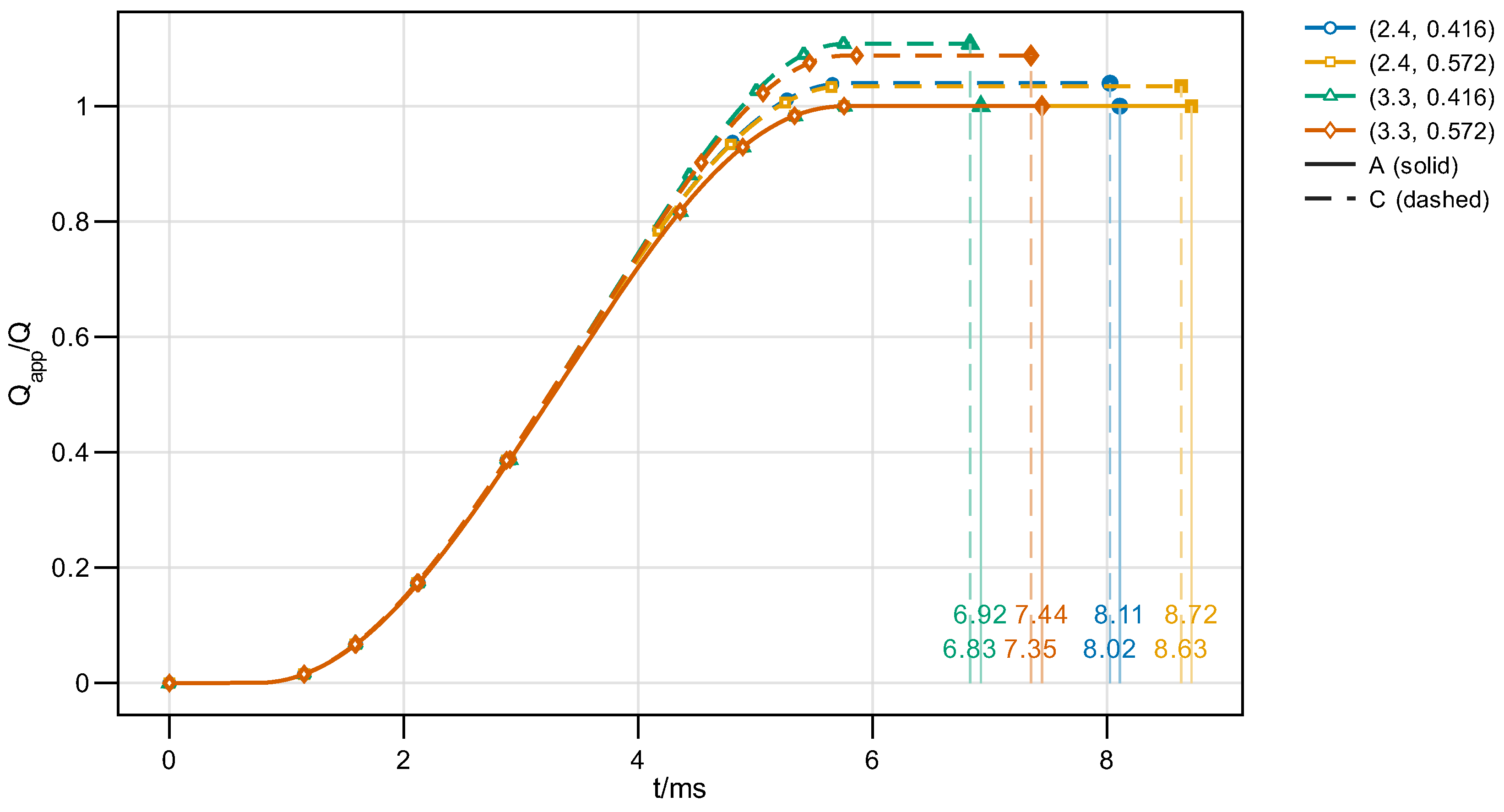
A and C share four $(Q,m_p)$ conditions. The two case classes keep the RNG k–$\epsilon$ flow closure, prescribed heat-release history, geometric motion, and numerical settings unchanged, except for the heat-source normalization volume, which is changed from $V_g\left(t\right)$ to $V_0$. Figure 5 shows the cumulative applied-energy offset induced by fixed-volume normalization.

Figure 5. Cumulative applied-energy offsets induced by fixed-volume normalization for four operating conditions. The legend lists the operating conditions.

In the figure, the solid and dashed lines of the same color nearly coincide during the early heat-release stage and gradually separate as the gas region expands, indicating that the difference in fixed-volume normalization arises during the energy-input stage and accumulates with the boundary motion.

To separate the effects of the gas-region expansion amplitude and the heat-release timing, let the normalized heat-release rate and the relative gas-region expansion be

$$g\left(t\right)={\displaystyle \frac{\dot{Q}\left(t\right)}{Q}},{\int }_0^{t_{\delta }}g\left(t\right)\mathrm{d}t=1,{\xi }_V\left(t\right)={\displaystyle \frac{V_g\left(t\right)}{V_0}}-1.$$

(32)

Denote the active heat-release time window by ${\mathcal{T}}_Q=\{t:\dot{Q}\left(t\right)>0\}$, and define the inner product and norm within this window as follows:

$${⟨f,h⟩}_Q={\int }_{{\mathcal{T}}_Q}f\left(t\right)h\left(t\right)\mathrm{d}t,{\parallel f\parallel }_{2,Q}={\left[{\int }_{{\mathcal{T}}_Q}{f}^2\left(t\right)\mathrm{d}t\right]}^{1/2}.$$

(33)

The applied-energy bias caused by fixed-volume normalization can be written as the inner product of the heat-release history and the boundary-expansion history:

$${\mathcal{C}}_{QV}={⟨g,{\xi }_V⟩}_Q={\int }_0^{t_{\delta }}g\left(t\right){\xi }_V\left(t\right)\mathrm{d}t={\displaystyle \frac{Q_{\mathrm{app},\mathrm{C}}-Q}{Q}}.$$

(34)

${\mathcal{C}}_{QV}$ is defined as the heat-source–boundary coupling strength; it is exactly equal to the applied-energy bias, not an empirical quantity inferred from terminal responses.

The heat-source–boundary temporal-overlap coefficient is further defined as follows:

$${\Omega }_{QV}={\displaystyle \frac{{⟨g,{\xi }_V⟩}_Q}{{\parallel g\parallel }_{2,Q}{\parallel {\xi }_V\parallel }_{2,Q}}},0\le {\Omega }_{QV}\le 1,$$

(35)

The corresponding coupling capacity is defined as follows:

$${\mathcal{A}}_{QV}={\parallel g\parallel }_{2,Q}{\parallel {\xi }_V\parallel }_{2,Q}.$$

(36)

The energy-input bias then admits the exact decomposition:

$${\mathcal{C}}_{QV}={\mathcal{A}}_{QV}{\Omega }_{QV}.$$

(37)

${\mathcal{A}}_{QV}$ denotes the potential coupling capacity formed jointly by the heat-release intensity and the boundary-expansion amplitude, and ${\Omega }_{QV}$ denotes the degree of overlap between the two histories within the active heat-release window. The former answers how large a normalization bias the gas-region expansion can form, and the latter answers how much of it effectively coincides with the heat-release history in time; their product gives the applied-energy bias. The condition-by-condition values are listed in Table 11.

Table 11. Coupling decomposition of heat release and boundary expansion.

Condition	${\mathcal{A}}_{\mathit{QV}}$	${\mathsf{\Omega }}_{\mathit{QV}}$	${\mathcal{C}}_{\mathit{QV}}$
$(2.4,0.416)$	0.12267	0.3241	0.03976
$(2.4,0.572)$	0.09676	0.3597	0.03480
$(3.3,0.416)$	0.30524	0.3542	0.10811
$(3.3,0.572)$	0.24039	0.3645	0.08762

The ${\mathcal{C}}_{QV}$ values in Table 11 agree with the applied-energy bias of C within integration accuracy, indicating that this input bias arises from the temporal coupling between the heat-release history and the gas-region expansion history. High Q and low $m_p$ produce larger boundary displacements during heat release, and ${\mathcal{A}}_{QV}$ rises from $0.09676$ to $0.30524$; by comparison, ${\Omega }_{QV}$ varies only within $0.3241$–$0.3645$. The growth of the energy-input bias over the present condition domain is therefore controlled mainly by the coupling capacity formed by the boundary-expansion amplitude, while the temporal overlap between heat release and boundary motion provides secondary modulation.

As ${\mathcal{C}}_{QV}$ increases from $3.48\%$ to $10.81\%$, the pressure-work bias increases from $2.49\%$ to $6.90\%$. Part of the excess input is retained as gas internal energy and flow energy and participates in the subsequent expansion; the remainder is converted into mechanical work through the base-pressure history. The increased pressure drives the projectile out of the barrel earlier, but the shortened action time does not offset the increased instantaneous power, and the muzzle velocity ultimately increases by $1.24$–$3.39\%$.

The physical mechanism of fixed-volume normalization is thus decomposed into two factors: the expansion amplitude that the gas region can reach during heat release determines the coupling capacity, and the relative timing of heat release and boundary motion determines the overlap coefficient; their product gives the applied-energy bias. This decomposition further explains why the same prescribed chemical energy produces different source-term normalization errors at different $(Q,m_p)$ conditions. The A–C relations above are established at the four corner conditions of the condition matrix and within the prescribed-source forward problem, in which the source profile does not respond to local pressure, temperature, or gas-region expansion; they therefore describe the tested conditions under the controlled source input rather than the full domain or explicit combustion coupling. Under explicit combustion coupling, the heat-release rate would respond to the local pressure, temperature, and gas-region expansion, and the input-end bias identified here would be modulated by this response; quantifying the modulation requires combustion-coupled cases.

4.4. Cross-Condition Response Stability of the Modeling Differences

The leave-one-out reconstruction gain $G_{j,Y}$ in Section 3.3 tests the difference relation between one modeling choice and one response quantity. This section treats B and C as modeling-choice variables and tests whether they can stably reconstruct response offsets once the main operating-condition trend has been removed. To further judge whether the differences exceed what the $(Q,m_p)$ condition variation itself can explain, the two first-order response representations are compared. The first retains only the operating-condition variables:

$$Y_i^{\left(0\right)}={\beta }_0+{\beta }_Q{\tilde{Q}}_i+{\beta }_m{\tilde{m}}_{p,i}+{\epsilon }_i,$$

(38)

The second adds the modeling-choice variables to the same operating-condition terms:

$$Y_i^{\left(1\right)}={\beta }_0+{\beta }_Q{\tilde{Q}}_i+{\beta }_m{\tilde{m}}_{p,i}+{\beta }_B{I}_{B,i}+{\beta }_C{I}_{C,i}+{\epsilon }_i.$$

(39)

Here, $\tilde{Q}$ and ${\tilde{m}}_p$ are standardized operating-condition variables, and $I_B$ and $I_C$ denote the modeling-choice variables of B and C, respectively; A serves as the baseline, with both variables equal to zero. Both representations are evaluated by leave-one-out reconstruction on the full 28-case matrix, using the mean absolute error:

$${\mathrm{MAE}}_k\left(Y\right)={\displaystyle \frac{1}{N}}{\displaystyle \sum _{i=1}^N}\left|Y_i-{\widehat{Y}}_{i,-i}^{\left(k\right)}\right|,k\in \{0,1\},$$

(40)

The explanatory gain of the modeling-choice variables is defined as follows:

$$R_Y={\displaystyle \frac{{\mathrm{MAE}}_0\left(Y\right)}{{\mathrm{MAE}}_1\left(Y\right)}}.$$

(41)

$R_Y>1$ indicates that adding the modeling-choice variables reduces the leave-one-out reconstruction error; $R_Y\approx 1$ indicates that the modeling-choice variables provide no stable additional reconstruction capability; and $R_Y<1$ indicates an increased error after the variables are added.

Table 12 gives the leave-one-out mean absolute errors of the two response representations and the corresponding explanatory gains. The errors retain the original units of the response quantities, so $R_Y$ is a dimensionless indicator comparable across response quantities.

Table 12. Response-reconstruction gains of the modeling-choice variables.

Response Quantity	Unit	${\mathbf{MAE}}_0$	${\mathbf{MAE}}_1$	${\mathit{R}}_{\mathit{Y}}$
$Q_{\mathrm{app}}/Q$	–	0.0190	0.00993	1.92
$p_{\mathrm{br},\max }$	MPa	1.614	0.964	1.67
$p_{b,\max }$	MPa	2.119	2.319	0.91
$W_p$	MJ	0.0373	0.00729	5.11
$t_{\delta }$	ms	0.0522	0.0498	1.05
$v_{\mathrm{muzzle}}$	$\mathrm{m}{\mathrm{s}}^{-1}$	39.81	9.52	4.18

The pressure work and muzzle velocity have the largest $R_Y$, $5.11$ and $4.18$, respectively; after the modeling-choice variables are added, the leave-one-out errors decrease by about $80.4\%$ and $76.1\%$. The pressure work integrates $A_b{p}_b\left(t\right)v_p\left(t\right)$ over time, and the muzzle velocity reflects the accumulation of pressure acting on momentum and kinetic energy; their high gains therefore correspond to adjacent responses in the same physical process rather than to two independent pieces of evidence. The value $R_Y=1.92$ for $Q_{\mathrm{app}}/Q$ indicates that the modeling-choice variables can still identify the input bias of fixed-volume normalization after the current first-order $(Q,m_p)$ main trend is removed.

The peak base pressure has $R_Y=0.91$: adding the variables increases the leave-one-out error by about $10\%$. The action time has $R_Y=1.05$, with the error reduced by only about $4.8\%$. Neither form a clear explanatory gain of the variables. The peak base pressure is controlled by the local pressure-wave phase and peak timing, and the action time is mainly determined by the overall motion timescale; thus, neither can reliably capture the full difference between the modeling choices. The peak breech pressure, with $R_Y=1.67$, shows some variable separation. Still, its gain is lower than that of the integral quantities, indicating that retaining modeling-choice information in peak responses depends on the observation location and the temporal structure of the pressure history.

$R_Y$ judges whether the modeling choices provide additional cross-condition explanatory capability, but it does not state in what proportion the upstream bias is reflected in the pressure work and terminal kinetic energy. For each common condition k, define the upstream discrepancy measures:

$${\delta }_{F,k}={\displaystyle \frac{{∥p_{\mathrm{br},k}^B\left(t\right)-p_{\mathrm{br},k}^A\left(t\right)∥}_2}{{∥p_{\mathrm{br},k}^A\left(t\right)∥}_2}},{\delta }_{E,k}={\displaystyle \frac{Q_{\mathrm{app},k}^C}{Q_{\mathrm{app},k}^A}}-1.$$

(42)

The corresponding downstream discrepancy measures are:

$${\delta }_{W,k}^{\left(j\right)}={\displaystyle \frac{W_{p,k}^j}{W_{p,k}^A}}-1,{\delta }_{K,k}^{\left(j\right)}={\displaystyle \frac{\frac{1}{2}{m}_{p,k}{\left[v_{\mathrm{muzzle},k}^j\right]}^2}{\frac{1}{2}{m}_{p,k}{\left[v_{\mathrm{muzzle},k}^A\right]}^2}}-1,j\in \{B,C\}.$$

(43)

Here, ${\delta }_F$ retains the overall breech-pressure-history bias induced by the laminar closure, ${\delta }_E$ denotes the applied-energy bias induced by fixed-volume normalization, and ${\delta }_W$ and ${\delta }_K$ denote the relative biases of the base-pressure work and terminal kinetic energy, respectively.

For input and response biases ${\delta }_X$ and ${\delta }_Y$, write

$$\ln \left|{\delta }_{Y,k}\right|=a_{XY}+{\mathsf{\Lambda }}_{XY}\ln \left|{\delta }_{X,k}\right|+e_k,{\mathsf{\Lambda }}_{XY}={\displaystyle \frac{\partial \ln |{\delta }_Y|}{\partial \ln |{\delta }_X|}},$$

(44)

The logarithmic transfer elasticity ${\mathsf{\Lambda }}_{XY}$ is obtained from Equation (44), and the cross-condition fit is evaluated as follows:

$$R_{XY}^2=1-{\displaystyle \frac{{\sum }_k{e}_k^2}{{\sum }_k{\left[\ln |{\delta }_{Y,k}|-\overline{\ln |{\delta }_Y|}\right]}^2}}.$$

(45)

Equation (45) evaluates the cross-condition fit of the scaling relation. ${\mathsf{\Lambda }}_{XY}$ denotes the relative change of the response-bias magnitude when the input-bias magnitude changes by $1\%$, and $R_{XY}^2$ denotes the proportion of cross-condition variation explained by a single scaling relation; the two characterize the relative sensitivity and structural stability of the difference transmission, respectively. The fitted elasticities and coefficients of determination are listed in Table 13.

Table 13. Transfer elasticity and goodness of fit of the modeling differences.

Choice	Input	Response	N	${\mathsf{\Lambda }}_{\mathit{XY}}$	${\mathit{R}}_{\mathit{XY}}^2$
B	${\delta }_F$	${\delta }_W^{\left(B\right)}$	8	0.391	0.209
C	${\delta }_E$	${\delta }_W^{\left(C\right)}$	4	0.907	0.9999
B and C	${\delta }_W^{\left(j\right)}$	${\delta }_K^{\left(j\right)}$	12	1.000	$>0.9999$

For B, ${\mathsf{\Lambda }}_{FW}=0.391$ and $R_{FW}^2=0.209$, indicating that a single norm of the breech-pressure history cannot stably predict the work bias. The flow closure changes the arrival time and attenuation of pressure waves and the pressure-buildup process near the projectile base; $W_p$ depends on the synchronous integral of $p_b\left(t\right)$ and $v_p\left(t\right)$ over the entire motion history, and pressure-norm biases of the same magnitude can produce different work biases depending on the phase and the moving-boundary velocity. Thus, the pressure work and muzzle velocity have a high $R_Y$. Still, no stable single-parameter scaling relation exists between the pressure norm and the pressure work: the influence of B is carried by the complete history structure.

For C, ${\mathsf{\Lambda }}_{EW}=0.907$ and $R_{EW}^2=0.9999$: a $1\%$ relative increase in the applied-energy bias raises the pressure-work bias by about $0.907\%$, and the scaling relation covers the four common conditions. In Section 4.3, ${\delta }_W$ is always smaller than ${\delta }_E$, indicating that the excess input is also distributed to gas internal energy, flow energy, and the expansion process; the near-unity elasticity and fit indicate that this energy-distribution ratio remains stable across the four tested conditions. C produces an amplitude bias at the input end, whose influence on the pressure work is therefore closer to proportional transmission than the history effect of B.

Over the 12 common conditions of B and C, ${\mathsf{\Lambda }}_{WK}=1.000$ and $R_{WK}^2>0.9999$ hold for the pressure-work bias and the terminal kinetic-energy bias. This is consistent with the overall balance by which base-pressure work is converted into projectile kinetic energy, indicating that the muzzle-velocity difference is the terminal expression of the pressure-work bias, rather than a second piece of evidence independent of the work process.

Thus, $R_Y$ answers whether the modeling-choice variables retain explanatory capability after the main operating-condition trend is removed, while ${\mathsf{\Lambda }}_{XY}$ and $R_{XY}^2$ answer whether the differences follow stable physical scalings. The laminar closure appears as a combination of high integral-response gain and low pressure-norm–work fit, reflecting the coupling among the pressure history, phase, and moving-boundary velocity; fixed-volume normalization appears as a near-proportional relation between the energy-input bias and the pressure-work bias, reflecting the direct control of work by the source-term amplitude. Peak pressure and action time show no comparably stable variable gain. They therefore cannot replace the pressure histories, applied energy, and pressure work as the primary audit quantities of modeling differences. These stability and scaling indicators are obtained from the first-order local reconstruction about the reference condition; they support cross-condition stability within the tested $(Q,m_p)$ domain, and conditions with substantially different projectile mass or energy would require intermediate sampling or higher-order terms.

5. Conclusions

To address the problem that CLGG terminal responses cannot identify the sources of internal model differences, this paper constructs a process-resolved model-choice attribution (PMCA) framework, which isolates the flow closure and the heat-source normalization volume in a shared forward problem and determines the onset and transfer of differences along energy input, pressure transport, moving-boundary work, and the ballistic endpoint. When the flow closure is changed, the applied energy remains unchanged; the difference first appears in the pressure-transport process and increases the base-pressure work by $9.37$–$10.84\%$ through the cumulative action of the pressure history and projectile motion. The initial-volume normalization first changes the applied energy, producing $3.48$–$10.81\%$ excess applied energy, which is converted into a $2.49$–$6.90\%$ pressure-work increment. The two modeling choices thus have different internal onsets, but both can be transmitted to the ballistic endpoint through moving-boundary work.

Cross-condition reconstruction shows that the applied energy, pressure histories, and base-pressure work stably retain the above differences at held-out conditions. In contrast, local peak pressures do not exhibit comparable stability. Terminal-response agreement, therefore, cannot prove the equivalence of internal models; compressible flows with volumetric heat sources and moving boundaries require input conservation, complete pressure histories, and boundary work jointly to test the physical-process consistency of a model. PMCA converts discrete modeling choices into locatable, traceable, and cross-condition-testable differences in response, providing a model-comparison approach beyond terminal matching for strongly coupled moving-domain computations.

The above attribution is obtained within the shared forward problem, the prescribed heat-release history, and the investigated $(Q,m_p)$ condition domain, and the present matrix identifies the individual effects of the two modeling choices. Adding combined cases in which the two choices are switched simultaneously will enable testing of model interactions. Further modeling and numerical variables—such as ignition, detailed combustion kinetics, higher-fidelity turbulence closures and convection schemes, the equation of state, and mesh resolution—will enable testing of the persistence of the attribution relation over a wider condition domain.

References

- Kruczynski, D.; Massey, D.; Milligan, R.; Vigil, E.; Landers, B.; Meneguzzi, M. Combustion Light Gas Gun Technology Demonstration; Technical Report ADA462130; U.S. Army Research Laboratory: Adelphi, MD, USA, 2007. [Google Scholar]
- Zhou, F.; Liu, N.; Zhang, X.Y.; You, X. 1D study of the detonation phenomenon and its influence on the interior ballistics of the combustion light gas gun. Def. Technol. 2020, 16, 341–347. [Google Scholar] [CrossRef] [Scilit]
- Deng, F.; Liu, N.; Zhang, X. Analysis on influence of propellant component on interior ballistics of combustion light gas gun. J. Ballist. 2012, 24, 90–93. [Google Scholar] [CrossRef]
- Deng, F.; Zhang, X.; Liu, N. Influences of ignition process and initial conditions on interior ballistic characteristics of combustion light gas gun. Explos. Shock Waves 2013, 33, 551–555. [Google Scholar] [CrossRef]
- Deng, F.; Zhang, X. Simulation of hydrogen–oxygen combustion of combustion light gas gun using detailed chemical kinetics model. Acta Armamentarii 2014, 35, 415–420. [Google Scholar] [CrossRef]
- Deng, F.; Zhang, X.; Liu, N. Simulation on the flow characteristics of multi-stage divergent combustion chamber of combustion light gas gun. Explos. Shock Waves 2015, 35, 409–415. [Google Scholar] [CrossRef]
- Zhou, F.; Liu, N.; Zhang, X. Numerical study of hydrogen–oxygen flame acceleration and deflagration to detonation transition in combustion light gas gun. Int. J. Hydrogen Energy 2018, 43, 5405–5414. [Google Scholar] [CrossRef] [Scilit]
- Sheu, T.W.H.; Lee, S.M. Analysis of combustion processes in a gun interior ballistics. Int. J. Comput. Fluid Dyn. 1995, 4, 57–71. [Google Scholar] [CrossRef] [Scilit]
- Heiser, R.; Garloff, J. Study on turbulence in interior ballistics flows. J. Propul. Power 1992, 8, 59–65. [Google Scholar] [CrossRef] [Scilit]
- Liu, N.; Deng, F.; Zhou, F.; Zhang, X. Modeling of combustion and propulsion processes of a new concept gun using a gaseous propellant. J. Theor. Appl. Mech. 2015, 53, 531–541. [Google Scholar] [CrossRef] [Scilit]
- Hu, B.; Wang, Z.; He, H.; Peng, S.J. Simulation for launch process of combustion light gas gun based on CFD. Ship Sci. Technol. 2022, 44, 180–184. [Google Scholar] [CrossRef]
- Guermonprez, G.; Gaillard, T.; Dupays, J.; Anthoine, J.; Demarthon, R. A methodology to simulate interior and intermediate ballistics with dynamic mesh technique and lumped parameter code. Def. Technol. 2025, 49, 447–464. [Google Scholar] [CrossRef] [Scilit]
- Ongaro, F.; Robbe, C.; Papy, A.; Stirbu, B.; Chabotier, A. Modelling of internal ballistics of gun systems: A review. Def. Technol. 2024, 41, 35–58. [Google Scholar] [CrossRef] [Scilit]
- Deng, X. A unified framework for non-linear reconstruction schemes in a compact stencil. Part 1: Beyond second order. J. Comput. Phys. 2023, 481, 112052. [Google Scholar] [CrossRef] [Scilit]
- Deng, X. A new open-source library based on novel high-resolution structure-preserving convection schemes. J. Comput. Sci. 2023, 74, 102150. [Google Scholar] [CrossRef] [Scilit]
- Deng, X.; Massey, J.C.; Swaminathan, N. Large-eddy simulation of bluff-body stabilized premixed flames with low-dissipative, structure-preserving convection schemes. AIP Adv. 2023, 13, 055014. [Google Scholar] [CrossRef] [Scilit]
- Hirt, C.W.; Amsden, A.A.; Cook, J.L. An arbitrary Lagrangian–Eulerian computing method for all flow speeds. J. Comput. Phys. 1974, 14, 227–253. [Google Scholar] [CrossRef] [Scilit]
- Thomas, P.D.; Lombard, C.K. Geometric conservation law and its application to flow computations on moving grids. AIAA J. 1979, 17, 1030–1037. [Google Scholar] [CrossRef] [Scilit]
- Farhat, C.; Geuzaine, P.; Grandmont, C. The discrete geometric conservation law and the nonlinear stability of ALE schemes for the solution of flow problems on moving grids. J. Comput. Phys. 2001, 174, 669–694. [Google Scholar] [CrossRef] [Scilit]
- Ray, S.E.; Tezduyar, T.E. Fluid–object interactions in interior ballistics. Comput. Methods Appl. Mech. Eng. 2000, 190, 363–372. [Google Scholar] [CrossRef] [Scilit]
- Tezduyar, T.E. Finite element methods for flow problems with moving boundaries and interfaces. Arch. Comput. Methods Eng. 2001, 8, 83–130. [Google Scholar] [CrossRef] [Scilit]
- Saadat, M.H.; Karlin, I.V. Arbitrary Lagrangian–Eulerian formulation of lattice Boltzmann model for compressible flows on unstructured moving meshes. Phys. Fluids 2020, 32, 046105. [Google Scholar] [CrossRef] [Scilit]
- Bhadauria, A.; Dorschner, B.; Karlin, I. Lattice Boltzmann method for fluid–structure interaction in compressible flow. Phys. Fluids 2021, 33, 106111. [Google Scholar] [CrossRef] [Scilit]
- Xiao, H.; Wu, J.L.; Wang, J.X.; Sun, R.; Roy, C.J. Quantifying and reducing model-form uncertainties in Reynolds-averaged Navier–Stokes simulations: A data-driven, physics-informed Bayesian approach. J. Comput. Phys. 2016, 324, 115–136. [Google Scholar] [CrossRef] [Scilit]
- Oberkampf, W.L.; Trucano, T.G. Verification and validation in computational fluid dynamics. Prog. Aerosp. Sci. 2002, 38, 209–272. [Google Scholar] [CrossRef] [Scilit]
- Peherstorfer, B.; Willcox, K.; Gunzburger, M. Survey of multifidelity methods in uncertainty propagation, inference, and optimization. SIAM Rev. 2018, 60, 550–591. [Google Scholar] [CrossRef] [Scilit]
- Krier, H.; Summerfield, M. (Eds.) Interior Ballistics of Guns. In Progress in Astronautics and Aeronautics; American Institute of Aeronautics and Astronautics: New York, NY, USA, 1979; Volume 66. [Google Scholar]
- Yakhot, V.; Orszag, S.A. Renormalization group analysis of turbulence. I. Basic theory. J. Sci. Comput. 1986, 1, 3–51. [Google Scholar] [CrossRef] [Scilit]
- Patankar, S.V.; Spalding, D.B. A calculation procedure for heat, mass and momentum transfer in three-dimensional parabolic flows. Int. J. Heat Mass Transf. 1972, 15, 1787–1806. [Google Scholar] [CrossRef] [Scilit]
- Issa, R.I. Solution of the implicitly discretised fluid flow equations by operator-splitting. J. Comput. Phys. 1986, 62, 40–65. [Google Scholar] [CrossRef] [Scilit]
- Sacks, J.; Welch, W.J.; Mitchell, T.J.; Wynn, H.P. Design and analysis of computer experiments. Stat. Sci. 1989, 4, 409–423. [Google Scholar] [CrossRef] [Scilit]
Disclaimer/Publisher’s Note: The statements, opinions and data contained in all publications are solely those of the individual author(s) and contributor(s) and not of MDPI and/or the editor(s). MDPI and/or the editor(s) disclaim responsibility for any injury to people or property resulting from any ideas, methods, instructions or products referred to in the content. |
© 2026 by the authors. Licensee MDPI, Basel, Switzerland. This article is an open access article distributed under the terms and conditions of the Creative Commons Attribution (CC BY) license.