


Abstract
Conceptual design is a critical phase in the development of propulsion plants. Its aim is to explore multidimensional design spaces to provide guidelines for the detailed design phase. This exploration is necessarily broad in scope and shallow in fidelity. Lately, developments in computing hardware have allowed the use of simplified computational fluid dynamics (CFD) models for conceptual design purposes, thereby increasing significantly the amount of data to be processed and generalised. In this context, the present work benchmarks two specific surrogate-model implementations for the conceptual design of a rocket-type pulse detonation engine: a tensor-based method based on high-order singular value decomposition (HOSVD) and a fully connected feed-forward neural network (NN). Two complementary comparisons were considered: HOSVD versus NN, using the same factorial databases to assess the effect of the surrogate method; and factorial versus low-discrepancy sampling, using the same NN architecture to assess the effect of the database distribution. The benchmark, which involved five input architecture parameters and five output operation parameters, was performed for both the direct analysis problem (outputs obtained from inputs) and the inverse design problem (inputs obtained from outputs). Three different situations were considered in the comparison—dimensionally balanced, overdetermined, and underdetermined—to simulate conditions that typically arise in these design phases. Three databases of different sizes were generated for the comparison. The results provide a case-specific assessment of the performance of the two implementations under the conditions considered and may provide useful guidance on the application of these data-analysis approaches in conceptual design.
1. Introduction
Conceptual design is a key phase of the development process of propulsion plants. Its objective is the exploration of a multi-dimensional space of design variables to provide guidelines for the detailed design phase. Typically, it involves computation of hundreds/thousands of cases, so it is based on the use of low-fidelity methods that are relatively inexpensive to compute. Those results, to be of any use, need to be organised and generalised efficiently. From a methodological standpoint, the goal is to extract a maximum of information out of data that could be described as very broad in scope and shallow in fidelity. In practice, despite the limitations of the conceptual design phase as compared to the detailed design phase, decisions taken at this early stage are seldom reversed later, thereby giving it importance in the industrial context.
For a long time, propulsion plant conceptual design relied on the method of gas path analysis and its many variants. However, approaches started to change significantly about 15 years ago when improvements on computing hardware allowed for the introduction of simplified CFD simulations into the process. This implied that the amount of data to be analysed increased dramatically since space/time distributions of variables (and not only global performance parameters) became available.
Nowadays, propulsion engineers could use a wealth of different methods for data analysis in the context of conceptual design. Broadly speaking, these methods could be classified as either algebraic-based or AI-based. Then, it might be of interest to define an application test point, apply both approaches on even grounds, perform a systematic comparison of the results, and draw indications that may help engineers to assess their portfolio of data analysis methods. This comparison cannot be of a generic nature because it depends on the selected propulsion plant architecture.
The propulsion plant selected for the present work is a rocket-type pulse detonation engine (PDE) with a convergent-divergent (Con-Di) nozzle. The reasons for the selection are twofold. First, it is a promising concept that has already expanded its reach out of the design board to enter the phases of extensive experimental testing and flight testing; see Bogoi et al. [1], Goto et al. [2], and Buyakofu et al. [3]. Second, the internal flow physics involved is reasonably complex: supersonic reacting flow (detonation wave) combined with strong unsteady effects.
Concerning traditional approaches to the conceptual design of PDE, Jie et al. [4] developed an evolved version of the ideal cycle thermodynamics analysis to study the performance of a PDE gas turbine. In the same field of application, Asli et al. [5] used a 1D CFD approach combined with blade source terms. Peace and Lu [6] employed a quasi-1D Method of Characteristics of low computational cost. Roux [7] evolved an idealised version of the PDE thermodynamics cycle. Hua et al. [8] superimposed 1D CFD simulations on some branches of the ideal cycle. The performance of a hydrogen-propelled PDE was studied by Luo et al. [9] using a modified ideal cycle. Tan et al. [10] analysed the transient operation characteristics of a PDE gas turbine by establishing balance equations for the different parts of the engine. Xiao et al. [11] adopted the viewpoint of exergy analysis in their study of the PDE cycle. Sanchez de Leon et al. [12] used 1D simulations involving a 25-chemical-reaction H2-air mechanism to generate a PDE surrogate model that could be used for both the direct (performance) and inverse (design) problems. Along the same line, Gonzalez-Viana et al. [13] employed a similar type of surrogate model for multi-objective optimisation of the PDE nozzle. Concerning AI approaches, there is a lack of references dealing with PDE. In fact, most AI studies address rotating detonation engines (RDE) that are the annular equivalent of the PDE. Wolff et al. [14] developed a neural network (NN) for misfiring detection purposes in an annular pulsed detonation combustor (a concept that is somewhat different from a conventional PDE). Johnson et al. [15] and Johnson et al. [16] used convolutional NN for wave mode identification and detonation identification, respectively, in RDE. Koch [17] developed an RDE surrogate using neural differential equations. Mendible [18] employed machine learning for rotating detonation wave modelling. Shen et al. [19] formulated an interpretable deep learning method to predict combustion performance in an RDE. Wang et al. [20] modelled a rotating detonation combustor via physics-informed NN, while Johnson et al. [21] used machine learning for RDE diagnosis.
The objective of the present study was to perform a systematic comparison of the accuracy, operational aspects, and general pros and cons of two different methods in the context of the conceptual design of a PDE. The first method was algebraic tensor-based (TB) that used the high-order singular value decomposition (HOSVD) approach, and the second was neural network based (NN). The idea was to provide the aerospace engineer with insights that might be of interest when managing a portfolio of different conceptual design methods. The authors are not aware of this type of comparison in the specialised literature regarding PDE propulsion plants.
HOSVD and feed-forward NN surrogates have not previously been benchmarked for pulse detonation engine conceptual design using common databases and test points for both direct and inverse problems. The specific contribution of this work is therefore not the development of either method but a controlled benchmark designed to separate the effect of the surrogate method from that of the sampling distribution. The benchmark also examines the influence of database size and to reduces the number of output parameters, thereby covering conditions of different dimensionality that may arise in conceptual design applications.
The benchmark was structured to distinguish between the effect of the surrogate method, assessed using the common factorial databases, and the effect of the sampling distribution, assessed using the NN algorithm.
As for the organisation of this article, the problem is defined in Section 2, while the CFD model that provides the data is described in Section 3. The TB and the NN formulations are described in Section 4 and Section 5, respectively; results and discussions are presented in Section 6; and, finally, conclusions are given in Section 7.
2. Description of the Problem
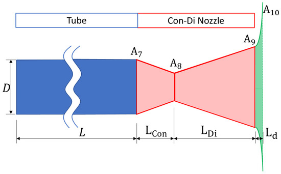
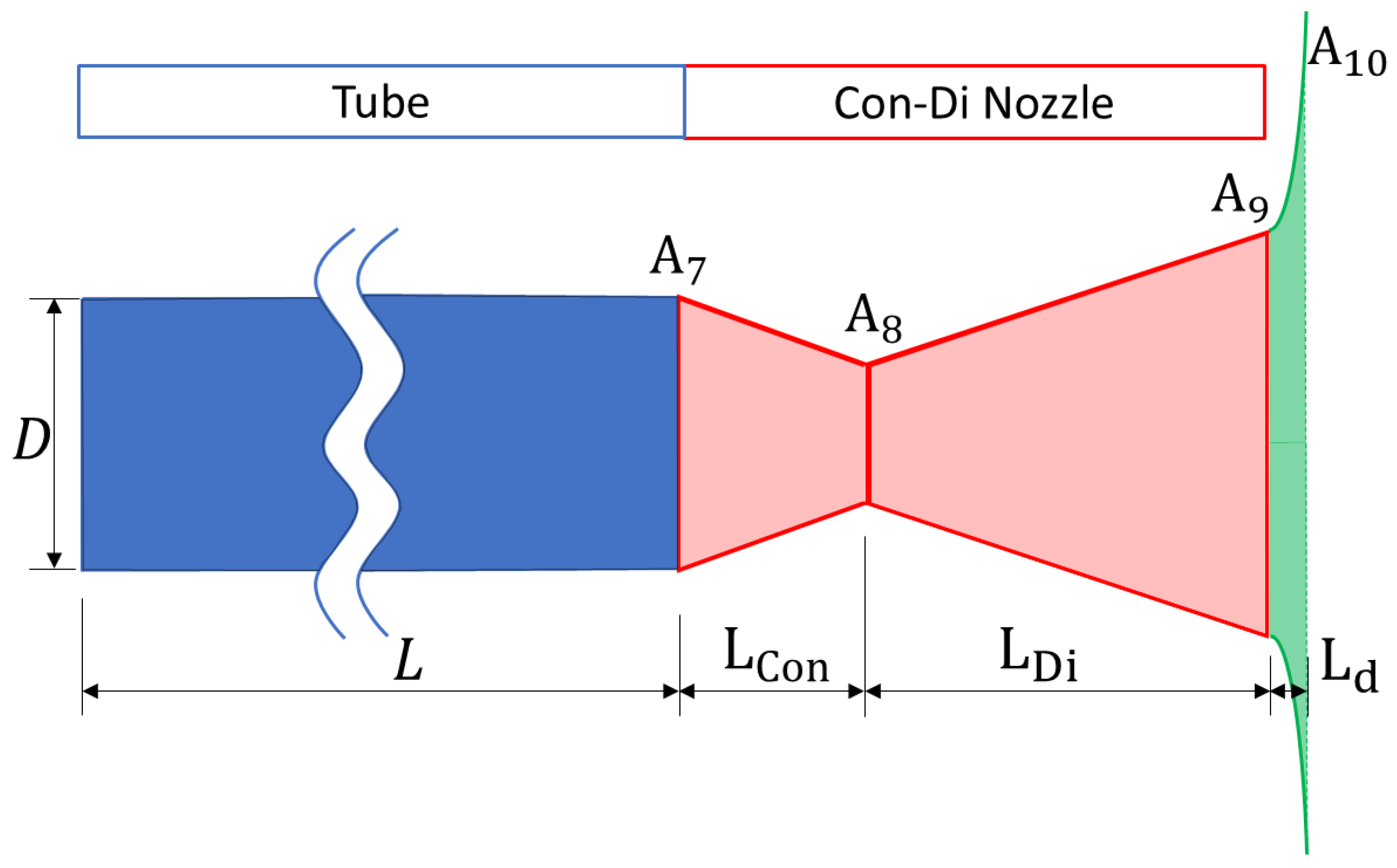
The problem consisted of comparing the performance (regarding data analysis and generalisation) of two approaches of different nature, TB and NN, in the context of the conceptual design of a rocket-type pulse detonation engine with a convergent-divergent (Con-Di) nozzle. The input for both methods was a multi-parameter, multi-dimensional database generated via computational fluid dynamics (CFD). A sketch of the PDE configuration is presented in Figure 1. The length and diameter of the circular section were constant: , .
Figure 1.
Sketch of the PDE configuration. Sections (A7, A8, A9) were named after the standard convention used in propulsion plants.
The numerical model for database generation was unsteady and quasi-1D with variable cross-section area . A simplified chemical kinetics model was used to describe the combustion of the H2-air mixture with four species and one irreversible global reaction. The problem had 5 input parameters () and 5 output parameters (). Input parameters were related to the PDE design while output parameters were connected to PDE operation. Their definition and nomenclature are presented in Table 1.
Table 1.
Input and output parameters of the problem.
Two different CFD databases, DB1A and DB1B, were generated first. DB1A was organised as a group of 5 tensors, whereas DB1B consists of a list of sparse low-discrepancy samples the same size as DB1A. Each tensor had 5 axes (the input parameters) and contained one output parameter. Each combination of five input parameters and their corresponding five output parameters is hereafter referred to as a “database sample”. Database DB1A contained 13,860 such samples. For the NN implementation, 95% of the database samples were assigned to the training set, while the remaining 5% constituted the validation set used for early stopping. In contrast, the complete factorial database was used to construct the HOSVD surrogate. The additional 1400 CFD evaluations described below constituted an independent test set—with each of those called a test point common to all the benchmarks—and were excluded for either NN training, validation, or HOSVD surrogate construction.
Database DB1A had a factorial distribution of input parameters. This distribution was as follows:
Database DB1A (5 × 6 × 11 × 7 × 6 = 13,860 database samples):
- , 5 values: 0.8, 0.9, 1.0, 1.1, 1.2;
- , 6 values: 1.0, 1.8, 2.6, 3.4, 4.2, 5.0;
- , 11 values: 1.0, 2.4, 3.8, 5.2, 6.6, 8.0, 9.4, 10.8, 12.2, 13.6, 15.0;
- , 7 values: 0.02, 0.05, 0.08, 0.11, 0.14, 0.17, 0.20;
- , 6 values: 1.0,1.8, 2.6, 3.4, 4.2, 5.0.
Throughout the manuscript, each complete set of input and output parameters is referred to as a database sample, whereas database denotes the complete collection of these samples.
Database DB1B had the same minimum and maximum limits for the input parameters and the same number of database samples as DB1A, but these were distributed using the quasi-random low-discrepancy Sobol method; see Sobol [22]. Details of the low-discrepancy approach are provided in Section 6: Results and Discussion.
The neural network method was applied to both the factorial and low-discrepancy databases, whereas HOSVD was applied only to the factorial database. Standard HOSVD requires the data to be arranged as a complete tensor whose entries correspond to factorial combinations of the input parameters. This condition is not met by the scattered samples of the low-discrepancy database. Gappy HOSVD can reconstruct missing entries when the available samples occupy known positions in an otherwise factorial tensor. It consists of the recursive application of HOSVD to an incomplete tensor and, to the authors’ knowledge, was first tested on an aerodynamic problem by Moreno et al. [23]. It was later applied to reconstruct an incomplete RDE performance database for conceptual design purposes by Sastre et al. [24]. In principle, a more extensive completion procedure could be developed to infer a full factorial tensor from low-discrepancy samples through an iterative optimisation process. However, since these samples do not coincide with the nodes of the target tensor, this would require an additional mapping procedure or a different tensor regression method rather than a direct application of Gappy HOSVD. This possibility was therefore considered outside the scope of the present benchmark.
Accordingly, the results were interpreted through two complementary comparisons. First, HOSVD and NN were compared using the same factorial databases (A cases) to assess the effect of the surrogate method under equivalent database conditions. Second, the NN results obtained with factorial and low-discrepancy databases containing the same number of samples (A and B cases, respectively) were compared to assess the effect of the sampling distribution.
To achieve maximum robustness of both the TB and NN methods, both input and output parameters were rendered dimensionless and scaled between 0 and 1 as follows:
To test the behaviour of both methods, 1400 additional test points were computed inside the parametric domain. These 1400 points did not coincide with any interior point of DB1A or DB1B and were the same for both databases. They were selected via the Latin hypercube sampling technique to ensure an even distribution inside the 5D spaces of parameters. Each of the 1400 test points had its own set of input and output parameters. Then, both the TB and the NN methods were used to compute the 1400 test points both for the direct problem (outputs obtained from inputs) and the inverse problem (inputs obtained from outputs). The average ( and maximum errors () between the exact computations and the results provided by the two methods were calculated. The definition of was as follows:
Subscripts and are the number of parameters and the number of points in the test sample. All errors reported in this work were calculated using the dimensionless variables normalised between 0 and 1 according to Equation (1). The values presented as percentages were obtained by multiplying these normalised errors by 100. stands either for a dimensionless output parameter (direct problem) or an input parameter (inverse problem).
For each problem, the absolute differences between the surrogate predictions and the CFD reference values formed a 1400 × 5 error matrix. While is the mean of all its entries, is the largest individual entry and therefore corresponds to one variable at one test point.
For the inverse problem, an additional reconstructed output error () was computed to complement the error associated with recovering the reference input parameters. Once an input set had been obtained from a given output query, the corresponding output set was calculated by evaluating the corresponding surrogate direct problem. The reconstructed output error was computed as defined in Equation (2), but compared with the output query . Thus, this metric represents the mean absolute deviation between the requested and reconstructed outputs in the normalised space and indicates how accurately the solution identified by the inverse method reproduces the requested engine performance.
Additionally, the comparison was repeated using four smaller databases. DB2A and DB2B contained 6000 samples with factorial and low-discrepancy distributions, respectively. DB3A and DB3B followed the same distributions and contained 2160 samples. The objective was to assess which method performed better in the context of increasing sparsity of information. The definitions of DB2A and DB3A were as follows:
Database DB2A (4 × 5 × 10 × 6 × 5 = 6000 database samples):
- , 4 values: 0.8, 1.0, 1.1, 1.2;
- , 5 values: 1.0, 2.6, 3.4, 4.2, 5.0;
- , 10 values: 1.0, 2.4, 3.8, 6.6, 8.0, 9.4, 10.8, 12.2, 13.6, 15.0;
- , 6 values: 0.02, 0.08, 0.11, 0.14, 0.17, 0.20;
- , 5 values: 1.0, 2.6, 3.4, 4.2, 5.0.
Database DB3A (3 × 4 × 9 × 5 × 4 = 2160 database samples):
- , 3 values: 0.8, 1.0, 1.2;
- , 4 values: 1.0, 2.6, 3.4, 5.0;
- , 9 values: 1.0, 2.4, 3.8, 6.6, 8.0, 9.4, 12.2, 13.6, 15.0;
- , 5 values: 0.02, 0.08, 0.11, 0.14, 0.20;
- , 4 values: 1.0, 2.6, 3.4, 5.0.
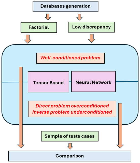
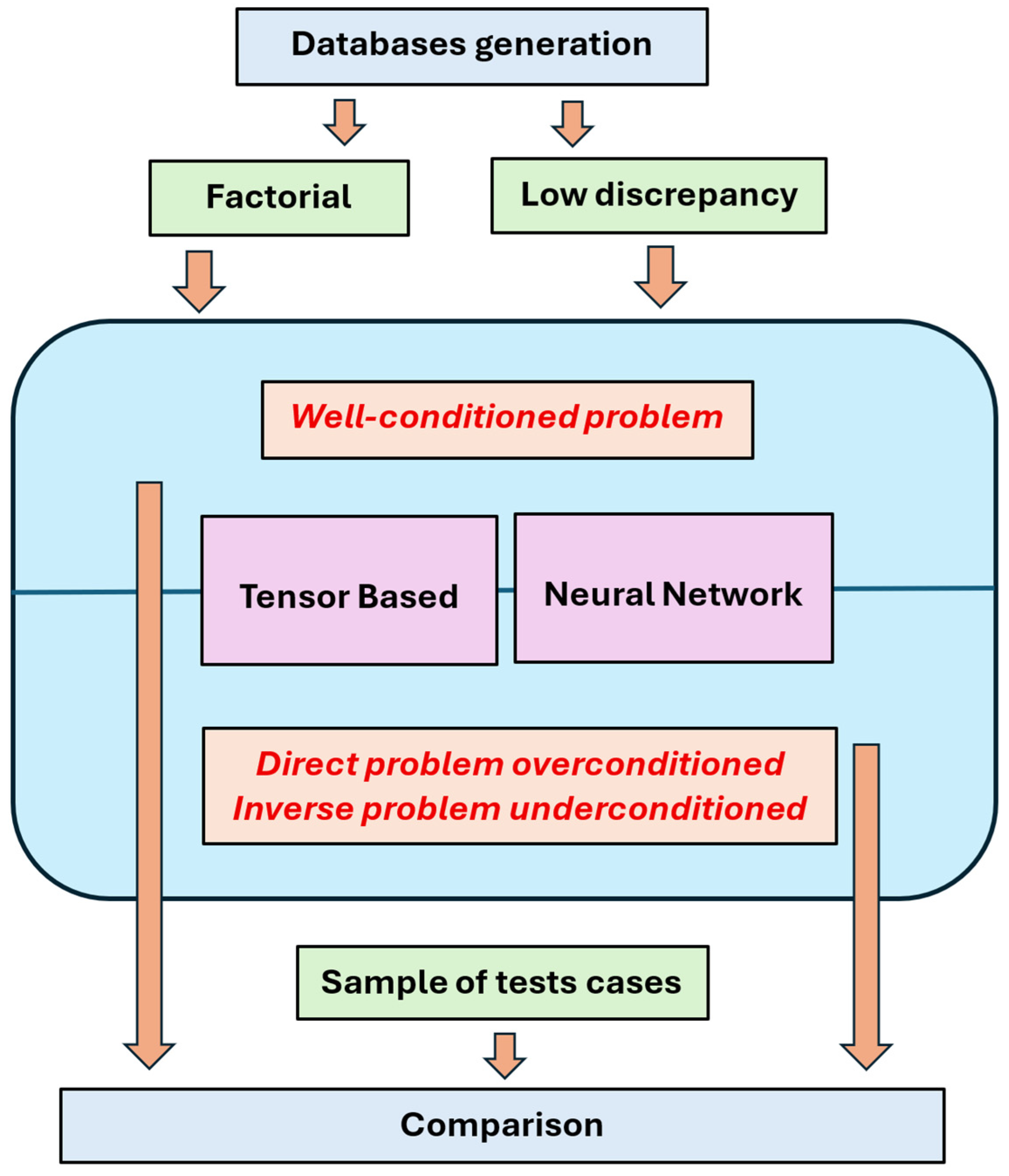
Finally, yet another two cases were computed that considered 5 input parameters ( to ) and 2 output parameters ( and ). The rationale for these cases was to include an overdetermined situation for the direct problem and an underdetermined situation for the inverse problem. The summary of cases and the nomenclature are presented in Table 2. For the sake of clarity of exposition, a sketch of the workflow described above is presented in Figure 2.
Table 2.
Nomenclature for the computed cases. F and LD refer to factorial and low-discrepancy databases, respectively. “tb” and “nn” stand for tensor-based and neural network, respectively. Case keys consist of a number identifying the test configuration, the letter A or B identifying the database distribution, and the suffix ‘tb’ or ‘nn’ identifying the method. Comparisons between Atb and Ann cases assess the method effect, whereas comparisons between Ann and Bnn cases assess the sampling-distribution effect.
Figure 2.
Sketch of the workflow.
3. Description of the Flow Solver
The quasi-1D unsteady compressible reactive Euler model described in Gonzalez-Viana et al. [13] was selected to solve the flow. JANAF polynomials, described by Stull and Prophet [25], were used to describe the thermal properties of each species in the H2-air gas mixture, while chemical kinetics were modelled by a one-step irreversible global reaction with the following Arrhenius reaction rate:
with the preexponential factor and activation temperature equal to and , respectively (McGough [26], Towery et al. [27], and Rai et al. [28]).
The 1D domain with variable cross section area included the PDE tube (), the Con-Di nozzle (), and a discharge section. Simulations were performed for various cross-sectional area distributions (Figure 1). The computational discharge section was times larger than that of the tube. It was modelled with a parabolic profile connected smoothly to the nozzle outlet to ensure numerical stability. The quasi-1D PDE domain was initialised at pressure and temperature and , and filled with a quiescent and air () mixture of different equivalence ratios (input parameter ). Ignition was prescribed at over one cell length with temperature and pressure equal to and , respectively. The nozzle and discharge sections initially contained air. Boundary conditions were zero velocity at the closed end, with zero gradients for other variables, and ambient pressure at the outlet with zero-gradient velocity and temperature. The governing reactive Euler equations were solved in OpenFOAM using a modified version of the rhoCentralFoam solver. Convective fluxes were discretised using the second-order central upwind scheme of Kurganov et al. [29]. Implicit Euler time integration and Newton–Raphson iterations were used for the flow and temperature equations, while chemistry was treated by operator splitting with a fourth order Runge–Kutta scheme. A uniform mesh of and adaptive time stepping with a maximum Courant number of 0.1 were employed after a sensitivity analysis (see Gonzalez-Viana et al. [13] for details). Simulations ended () when the static pressure at returned to .
The thrust time integral and the fuel based specific impulse were calculated, respectively, as , and , where is the initial mass of fuel inside the PDE tube.
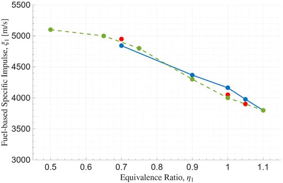
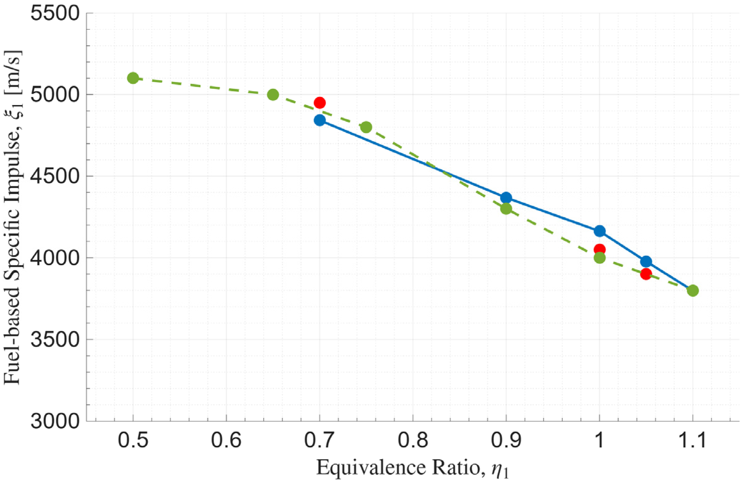
To assess the accuracy of the single-step irreversible reaction scheme, results for a stoichiometric mixture were compared with NASA CEA predictions at the Chapman–Jouguet (CJ) point. Deviations were small: +1.5% in CJ pressure, +2.7% in wave speed, and +10% in temperature—the latter reflecting the absence of intermediate chemistry and heat-absorbing species. The solver’s performance prediction was further examined by computing the fuel-based specific impulse for different equivalence ratios and contrasting it with experimental data from Schauer et al. [30] and numerical results from Sánchez de León et al. [12], as depicted in Figure 3. The agreement was good near stoichiometric and rich mixtures, although the model could not capture detonations at very lean conditions (with equivalence ratios < 0.7) due to the simplified chemistry. As a third validation case, the configuration analysed by Ornano et al. [31], using the Method of Characteristics, was reproduced. The steady thrust obtained with the present model was 5865 N, compared to 5960 N reported by Ornano et al. [31], corresponding to a deviation of about 2%. Finally, an unsteady case adapted from Owens and Hanson [32] reproduced detonation-driven nozzle flow, with discrepancies below 7% in maximum thrust, wave arrival time, and blowdown duration. Overall, the solver showed reliable predictive capability for detonation properties and performance metrics, despite the simplifications in chemical kinetics.
Figure 3.
Fuel-based specific impulse comparison between the present model (blue dots), and the works of Sanchez de Leon et al. [12] (numerical, red dots) and Schauer et al. [30] (experimental, green dots).
The validation and numerical sensitivity of the CFD framework are summarised above and reported in further detail in Gonzalez-Viana et al. [13]. Additional pointwise comparisons at the centre or other interior locations of the 5D tensor could not be performed because, to the authors’ knowledge, no published experimental or higher-fidelity numerical results are available for the specific PDE and nozzle geometries represented by these points. The available reference cases therefore provide the closest feasible validation, while the conclusions are then restricted to the ability of these approaches to reproduce and invert the numerical mapping generated by the quasi-1D CFD model.
4. Description of the Algebraic Tensor-Based Model
The algebraic-based model consisted of three phases: (a) generation of the initial database (as described in Section 2), (b) construction of a surrogate model, and (c) development of the algorithm to compute both the direct and inverse problems.
The first phase (a) was performed offline. For this algebraic-based model, discretisation must follow a factorial mesh. Once generated, the database underwent a high-order singular value decomposition (HOSVD) postprocessing to build a surrogate model of the original database. This surrogate exposed and exploited the underlying patterns of the database to facilitate the development and operation of the direct/inverse algorithm (phase (c)). The postprocessing of the database began with the application of the HOSVD, Tucker [33], and Lathauwer et al. [34,35]. No truncation was applied to the HOSVD in the present study. All singular vectors and the complete core tensor were retained for each output database. Consequently, the decomposition itself introduced no approximation error at the original database points. The next step involved generation of cubic splines between the nodes of all eigenvectors, allowing for interpolation in the HOSVD modal space. This allowed for the accurate reconstruction of outputs even if none of the inputs coincided with the original database entries (in between the factorial mesh). The final step consisted of developing and operating an optimisation algorithm for the inverse problem. For this purpose, the MATLAB (R2025a) function FMINCON was employed. This is a gradient-based, iterative interior-point method that, like most algorithms of its class, requires an initial guess to initiate the iterations.
An important feature of the methodology is that the output query does not need to be consistent with the model. In other words, it does not have to lie within the algebraic image of the surrogate. Nevertheless, all test points considered here were computed using the original model and were therefore consistent with its image. Though naturally, these TCs were not part of the database used to construct the surrogate.
To improve convergence, the starting point for the optimisation should ideally belong to the surrogate’s image. For this reason, a set of 1200 sampling points was generated in advance using Latin hypercube sampling in the 5D domains and was stored as part of the surrogate model together with the splines and the core tensor. The initial guess was chosen as the point whose outputs were closest to the query with the Euclidean norm. The optimisation itself proceeded through the interior-point algorithm, which minimised the distance between the model outputs and the query while keeping the model’s constraints. The method generated local approximations for the objective function, applied a barrier term for stability, and progressively reduced this barrier to approach the feasibility boundary. Iterations continued until convergence criteria were satisfied. Readers seeking further details on this method are referred to Byrd et al. [36,37] and Waltz et al. [38].
5. Description of the Neural Network Configuration
The fully connected, multi-input, multi-output, feed-forward, multi-layer configuration was chosen for the NN. A calibration process was performed to select the configuration parameters (hidden layers and neurons). The candidate architectures were selected to have comparable numbers of trainable parameters, corresponding to 5–10% of the samples available in the largest database. This ratio was used only as a practical guideline, consistent with the order of magnitude found in research studies dealing with propulsion/power plants like gas turbines (Cao et al. [39], Manatura et al. [40], Hashmi et al. [41], Raghavan et al. [42], and Talebi et al. [43]). The calibration was performed using the largest database with 13,860 samples. The activation function was the hyperbolic tangent. This function is symmetric with zero average, so it is well suited to deal with normalised data (LeCun et al. [44]). Initialisation of unknowns was carried out using the method described by Glorot and Bengio [45].
The mean squared error (MSE) was used as the loss function. Adam was selected as a computationally efficient first-order optimiser that provides adaptive updates based on estimates of the first and second moments of the gradients (Kingma and Ba [46]). Although Adam was originally introduced for stochastic optimisation, it can also be applied in full-batch mode, as considered here and in the analysis of regression and scientific computing problems by Ma et al. [47]. The learning rate was set to 0.001, following the value recommended by Kingma and Ba [46]. The non-default values β1 = β2 = 0.99 were adopted because Ma et al. [47] showed that the conventional values β1 = 0.9 and β2 = 0.999 may produce spikes in full-batch problems with quadratic loss, whereas similar values of the two momentum factors provide smoother and more stable convergence. These parameters were kept unchanged for all NN configurations and databases to ensure a consistent comparison.
For NN training, 95% of the samples in each database were assigned to the training set, while the remaining 5% constituted the validation set. Full-batch training was employed, meaning that all database samples were used in every epoch. The maximum number of epochs was set at 50,000. Early stopping was applied by monitoring the validation loss and interrupting the training when it failed to show sufficient improvement according to the criterion described below. After an initial period of 2000 epochs, the validation MSE was compared at each epoch with its mean over the preceding 2000 epochs. Training was stopped after 100 consecutive epochs without an improvement exceeding the adaptive threshold. The counter was reset whenever improvement occurred.
For a fixed data split and weight initialisation, the training process was deterministic. However, the initial weights were randomly generated using the Glorot method [45]. Therefore, each network was trained five times using different initialisations, and the one producing the lowest validation loss was retained. The difference in average error between the best and worst runs was approximately 0.25% for the direct factorial case and 0.05% for the direct low-discrepancy cases, whereas for the inverse problem, it reached 4% with factorial sampling but remained around 0.05% with low-discrepancy sampling, indicating substantially more consistent training in the latter case, possibly aided by early stopping.
Three different NN configurations with a similar number of unknowns (weights and biases) were considered: #C1: 1 hidden layer, 60 neurons; #C2: 2 hidden layers, 20 neurons per layer; #C3: 3 hidden layers, 15 neurons per layer. In all three cases, the ratio of unknowns to database samples was on the order of 5%. When using databases DB2A, DB2B, DB3A and DB3B, the ratio increased to about 12% and 32%, respectively. These configurations were like others already studied in the propulsion/power specialised literature. In particular, C3 (5 inputs, 5 outputs, 3 hidden layers, 15 neurons per layer) was like the one proposed by Cao et al. [39] (8 inputs, 4 outputs, 3 hidden layers, 10 neurons per layer). In the case of Cao et al. [39], the ratio of unknowns to database samples was 6%. Table 3 shows a summary of the results obtained during the NN calibration process for the highest density databases (13,860 database samples). It could be observed that, except for the outliers (maximum error) for the factorial database, the three configurations, #C1, #C2, and #C3, had similar levels of errors. Then, in line with the work of Cao et al. [39], configuration #C3 was selected (3 hidden layers, 15 neurons per layer).
Table 3.
Comparison of the three NN configurations results in the case of the largest database (13,860 database samples). F and LD stand for factorial and low-discrepancy types of databases, respectively. and are the average error (defined in Equation (2)) and the maximum error, respectively. Since the NN architecture was kept unchanged in each row, the differences between the F and LD results are associated with the sampling distribution.
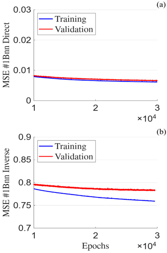
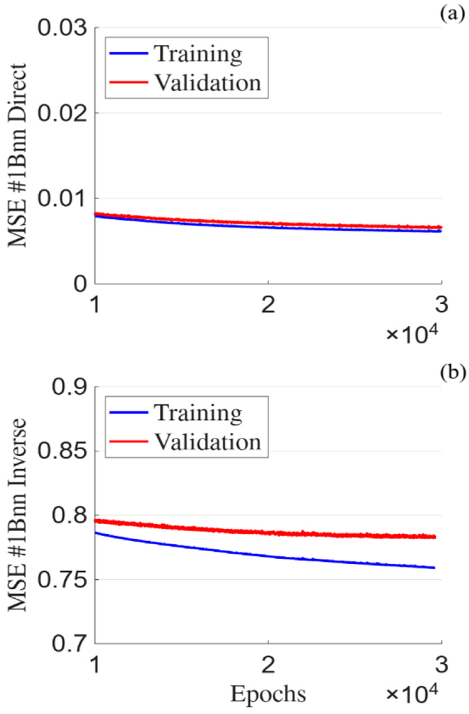
A different behaviour was observed for the inverse problems using low-discrepancy databases, for which the validation loss progressively flattened while the training loss continued to decrease, producing a growing generalisation gap. Early stopping was activated at epochs 19,681, 11,039, and 3748 for inverse cases #1Bnn, #2Bnn, and #3Bnn, respectively. This contrast is illustrated in Figure 4 through the late-stage training and validation MSE histories for the direct and inverse #1Bnn cases: for the inverse case, training was intentionally continued to epoch 30,000, beyond the early stopping point, to make the progressive flattening of the validation loss and the widening generalisation gap visible.
Figure 4.
MSE for direct (a) and inverse (b) training of #1Bnn.
Table 4 compares the inverse problem errors obtained for cases #1Bnn–#3Bnn when training was stopped at epoch 19,681 and when it continued until the maximum of 50,000 epochs, using the same data split and initialisation. The average error remained practically unchanged, whereas the maximum error increased when early stopping was disabled. Thus, early stopping had little influence on the overall predictive performance but prevented the deterioration of a small number of individual predictions.
Table 4.
Early stopping vs. no early stopping performance.
To assess whether the early-stopping behaviour observed for case #3Bnn was caused by the larger unknowns to database samples ratio, an additional NN configuration with 3 hidden layers and 4 neurons per layer was tested. This architecture contained 89 trainable parameters, resulting in a ratio of approximately 4.3%, close to the 5% obtained for case #1Bnn. However, no appreciable changes were observed in either the average or maximum errors compared with the original 3 × 15 architecture, and early stopping was still activated. Therefore, the detailed results of this additional configuration are not included, and the original architecture was retained to preserve consistency across the benchmark cases.
The robustness of the results with respect to the validation split was also examined for case #1Bnn. Validation fractions of 5%, 10%, and 20% were considered, and three different subsets were selected for each fraction. As summarised in Table 5, no appreciable variations were observed in the average error. Therefore, within the examined range, the results were not significantly affected by either the size or the particular composition of the validation set.
Table 5.
for #1Bnn with 5% to 20% validation cases for three different repetitions.
6. Results and Discussion
The global results obtained for both the direct and inverse problems are summarised in Table 6. The results are discussed through two independent comparisons. The Atb-Ann comparison isolates the effect of the surrogate method under the same factorial database conditions, whereas the Ann-Bnn comparison assesses the effect of the sampling distribution using the same NN implementation.
Table 6.
Results and nomenclature for the computed cases. F and LD refer to factorial and low-discrepancy database, respectively. “tb” and “nn” stand for tensor-based and neural network, respectively.
The following aspects could be observed:
- Direct problem. Average error. Cases #1Atb, #1Ann, and #1Bnn.
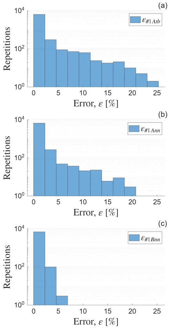
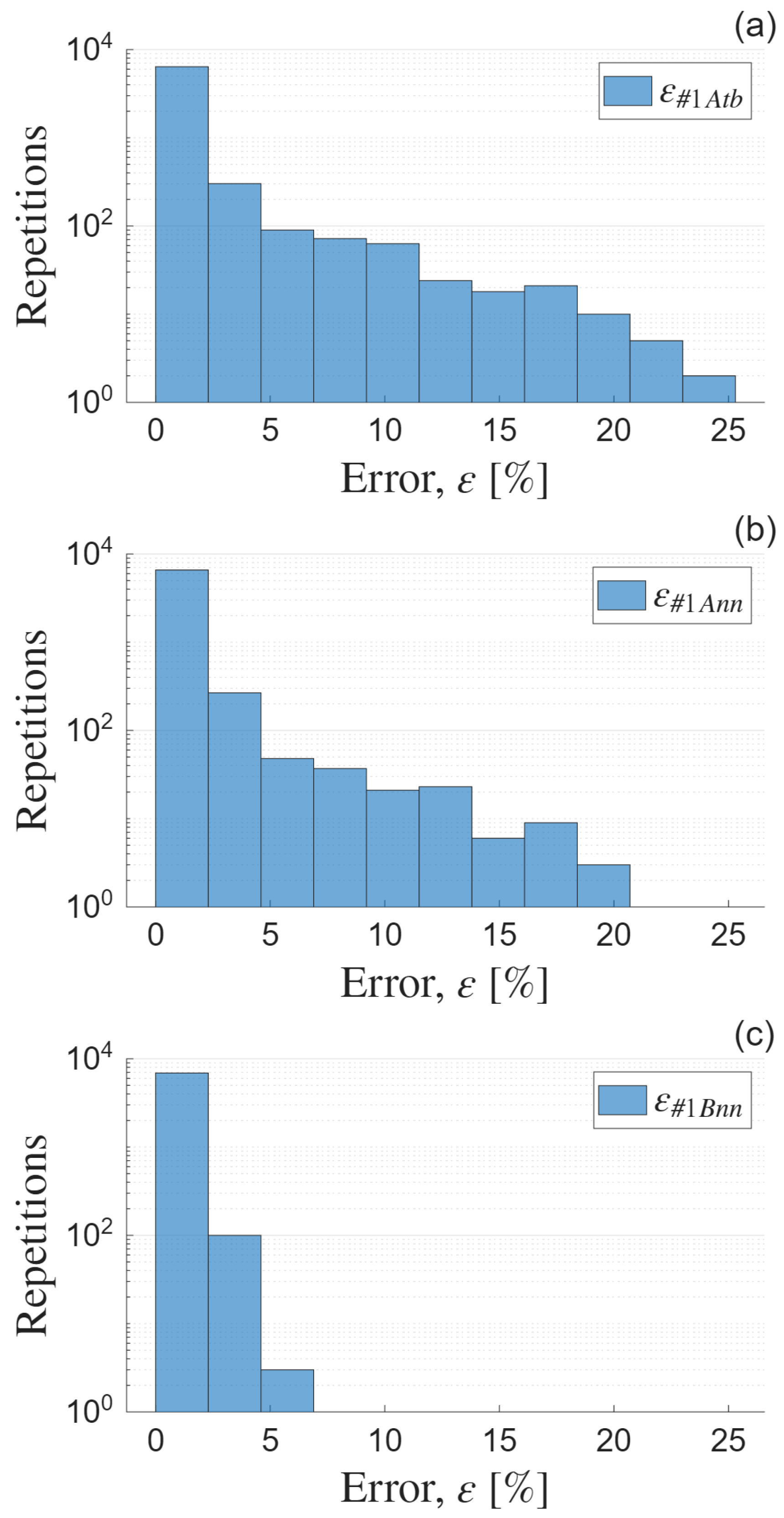
The average error was, in all cases, of the order of 1%, which is acceptable for conceptual design purposes. Regarding the surrogate method effect, a comparison of #1Atb and #1Ann shows that both algorithms produce a 1% average error. Regarding the sampling effect, a comparison of #1Ann and #1Bnn shows a reduction to 0.5% when using the low-discrepancy database. Furthermore, between 96% and 100% of all individual cases had errors below the 5% threshold, and between 98% and 100% of cases had errors below 10%; see Table 7. This suggests that the histograms of the distributions were slanted strongly towards the smaller errors, as illustrated in Figure 5. The conclusion is that, when looking at the average error, the specific HOSVD and NN implementations delivered a similar performance, provided that the database was dense enough. And, regarding the NN, this happened no matter whether the database had a factorial or a low-discrepancy distribution. This result was somewhat expected because both methods are “interpolating methods” that have proved their accuracy in many other contexts. Then, similar performance should not be a surprise.
Table 7.
Distribution of errors (direct problem) for all computed cases.
Figure 5.
Histograms for the error (in %) of cases. (a) #1Atb. (b) #1Ann. (c) #1Bnn. The number of repetitions is expressed in the log scale.
It is also relevant to have information about the mean error associated with individual outputs, , to see if any of them were more difficult to predict than the others. This information is shown in Table 8, where it could be observed that values of were similar for all outputs.
Table 8.
Distribution of average errors per output variable, , for the direct problem.
- II.
- Direct problem. Maximum error. Cases #1Atb, #1Ann, and #1Bnn.
Larger differences were observed in the maximum error . In particular, and for cases #1Atb and #1Ann (different algorithm, same database), respectively. However, by switching to the low-discrepancy database, the NN achieves , for case #1Bnn. The question is whether these outliers are, in practice, significant or not. The far-right column of Table 7 shows the percentage of cases in which error per test point exceeded the 15% threshold. It could be observed that the number of points exceeding the 15% error threshold was almost negligible.
- III.
- Inverse problem. Average error. Cases #1Atb, #1Ann, and #1Bnn.
For the inverse problem, increased to values of the order of 10% (Table 6). Errors of this magnitude are consistent with those reported in other aerospace conceptual design applications; for example, Dababneh and Conway-Smith [48] found predictions within approximately ±12% of the actual values in 62% of the analysed cases and considered this accuracy adequate for most conceptual and preliminary design purposes.
Differences in between the different cases were small: both algorithms with the DB1A achieve 10% average error, and NN using DB1B lowers it to 7%. Inverse problem errors (10%) were larger than direct problem errors (1%). The reason for this phenomenon could be related to the morphology of the image set in the 5D output spaces: two or more distinct input sets may produce output sets that are very close to each other. Consequently, when the algorithm is queried with a given output, it may identify an alternative input set that yields an output very similar to the query, while the solution input set is relatively distant from the correct one. An impression of the distribution of errors is presented in Table 9. It could be observed that the percentage of cases with an average error smaller than 20% was approximately 80%.
Table 9.
Distributions of errors (inverse problem) for all computed cases.
As shown by the reconstructed output errors included in Table 6, the output sets generated from the input parameters predicted by the inverse methods remained very close to the corresponding queries. These deviations were substantially smaller than the errors obtained when comparing the predicted and reference input parameters, which were generally of the order of 10% or higher. This indicates that noticeably different combinations of input parameters can produce very similar output responses. Consequently, a relatively large input recovery error does not necessarily imply that the identified design reproduces the requested performance poorly. For this reason, the reconstructed output error provides a complementary and, from an inverse design perspective, particularly relevant measure of solution quality.
Regarding the different predictions of input parameters, the average errors are presented in Table 10. While prediction of (equivalence ratio), (Con-contraction ratio), and (Di-expansion ratio) was carried out with errors smaller than 5% typically, the errors associated with (nozzle length ratio) and (Con/Di length ratio) were of the order of 10% and 20%, respectively. The reason could be that these input parameters do not have a significant impact in the evaluated outputs since it is possible to obtain similar results with very different and . In other words, the outputs have lower sensitivity to these two input parameters.
Table 10.
Average errors associated with the prediction of the different input parameters in the inverse problem.
To quantify the influence of each input parameter, the normalised Jacobian was evaluated at 100 points distributed throughout the parametric domain using Latin hypercube sampling. The derivatives were computed using centred finite differences, and Table 11 reports their root mean square values. The RMS formulation prevents derivatives with opposite signs at different locations from cancelling each other.
Table 11.
RMS of Jacobians calculated at 100 different locations of the parametric space.
The results show that has consistently the lowest influence on the outputs, while the sensitivity to is also lower than that associated with and . The median condition number of the normalised Jacobians was 551, and 97% of them had condition numbers above 100, indicating that the inverse mapping is locally ill-conditioned throughout most of the domain. Consequently, different input combinations may produce very similar outputs, explaining why relatively large input recovery errors can coexist with very small, reconstructed output errors.
- IV.
- Inverse problem. Maximum error. Cases #1Atb, #1Ann, and #1Bnn.
The maximum error for the inverse problem was of the order of 100%. Again, the question here is whether the outliers are significant or not. The far-right column of Table 9 shows that the percentage of cases with errors larger than 30% could be considered as a threshold for conceptual design applications in the context of the inverse (design problem).
For the HOSVD inverse cases, the optimisation performed with FMINCON was constrained to the normalised interval [−0.05, 1.05]. These bounds extend 5% beyond the original [0, 1] domain to allow limited extrapolation. Consequently, an error of 105% may occur when, for a particular test point and input parameter, the reference value lies at one boundary of the original domain (0 or 1), while the optimisation converges to the opposite extended boundary (1.05 or −0.05). In contrast, no explicit bounds or output clipping were imposed on the inverse NN predictions, which were evaluated directly as returned by the network. Predictions outside the normalised domain can therefore produce maximum errors exceeding 100%, including the values above 200% and 300% observed for some factorial NN cases. However, these extreme errors corresponded to isolated outliers representing only a negligible fraction (<0.1%) of the evaluated test points, and, consequently, they had a strong influence on the maximum error but little effect on the average error or the overall error distribution. Nevertheless, the substantially lower maximum error of 68% obtained for case #1Bnn is noteworthy, particularly because it was achieved without imposing explicit bounds on the NN outputs.
- V.
- Sparser databases. Cases #2Atb, #2Ann, #2Bnn, #3Atb, #3Ann, #3Bnn
Table 6 shows that reducing the number of database samples by factors of approximately 2 and 6 had only a limited effect on the direct problem errors. Regarding the surrogate method comparison under the same factorial database conditions, HOSVD and NN retained comparable accuracy across the three database sizes. Regarding the sampling distribution effect within the NN approach, both distributions remained stable, although the low-discrepancy databases consistently produced lower errors. A different trend was observed for the inverse problem. Under factorial conditions, the HOSVD results remained approximately unchanged, whereas the average error of the NN increased from 10% to 17–18% as the database size was reduced. In contrast, the NN trained with the low-discrepancy databases maintained average errors of approximately 7% and maximum errors between 68% and 72%. Thus, for the inverse problem considered here, low-discrepancy sampling made the NN less sensitive to reductions in database size.
- VI.
- Overdetermined and underdetermined cases: #4Atb, #4Ann, #4Bnn
All three approaches performed consistently better with the overdetermined direct problem than with the dimensionally balanced direct problem. Under the same factorial conditions, the HOSVD and NN implementations showed comparable trends, as average errors decreased slightly (see Table 6): from about 1% to 0.5%. For the NN algorithm, the low-discrepancy database also reduced the errors by around a half. Maximum errors decreased significantly: from about 20% to 3% for both the TB and NN approaches with the factorial database, and from 6% to 1% for the NN approach with the low-discrepancy database. All three approaches degraded consistently for the underdetermined inverse problem as compared to the dimensionally balanced inverse problem. Average errors nearly doubled (maximum errors did not change significantly).
- VII.
- Factorial versus Low-Discrepancy databases distributions
When generating database samples for surrogate models or neural networks, the distribution of sampling points across the parametric space influences the predictive performance of the resulting model. A common approach in engineering design is to use a factorial grid. Another approach is to use low-discrepancy sequences, such as the Sobol sequence introduced by Sobol [22]. These sequences are constructed deterministically to achieve a highly uniform coverage of the parameter space. The quality of coverage is quantified by the star discrepancy (Niederreiter [49]), D*, which measures the maximal deviation between the empirical distribution of the sampled points and the ideal uniform distribution. Lower values of D* indicate a more uniform distribution of points.
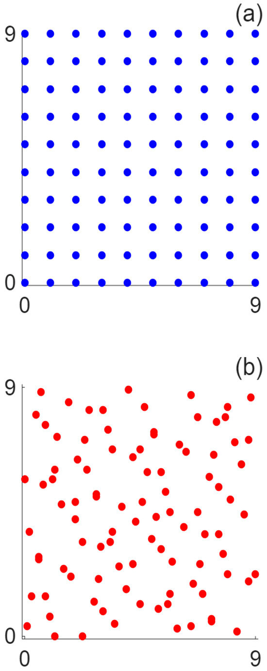
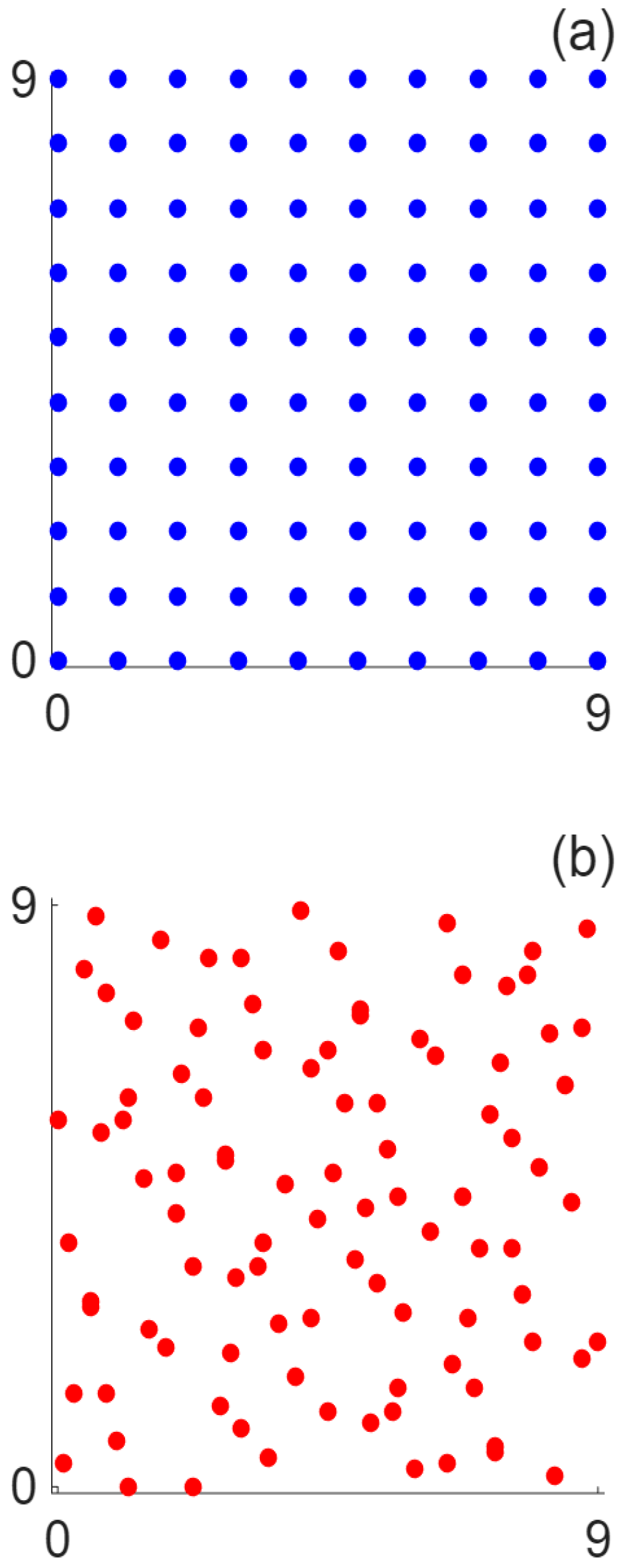
The discrepancy of a set of points is the maximum difference between the fraction of samples contained in an axis-aligned box anchored at the origin and the fraction of the domain volume occupied by that box. In other words, it is defined as the largest possible difference between two ratios: (a) the fraction of points that fall inside an axis-aligned box anchored at the origin, and (b) the fraction of the total domain volume that this box occupies. To illustrate this concept, two sets of 100 points in a 2D domain are compared: a uniform factorial 10 × 10 grid and a Sobol sequence; see Figure 6.
Figure 6.
Distribution of points for a factorial 10 × 10 mesh. (a) Factorial Distribution point list in a generic domain. (b) Sobol Distribution point list in a generic domain.
The factorial grid yields a star discrepancy of D* = 0.17, whereas the Sobol set achieves D* = 0.05. That is, sets with lower discrepancy inherently provide more information per sample, leading to better surrogate model training. Additionally, recent works have shown that training NN using low-discrepancy samples improves generalisation and reduces the number of required database samples. For instance, Mishra and Rusch [50] reported enhanced accuracy in deep learning algorithms when using low-discrepancy sequences for training data generation.
- VIII.
- Computational cost
The generation of the CFD databases represented, by far, the largest computational cost. A single CFD simulation required approximately 40 min. The two databases containing 13,860 samples each were generated in parallel using two workstations equipped with AMD Ryzen 9 9950X processors (Santa Clara, CA, USA), with 60 simultaneous processes. Consequently, their generation required close to two weeks per database. In comparison, the computational costs associated with the surrogate models were relatively small. For the NN, one full-batch training epoch required approximately 20 ms, resulting in about 15–20 min for a standard training of 50,000 epochs. Since five different weight initialisations were considered, the complete selection process required approximately 75–90 min per NN configuration. A single direct or inverse NN evaluation required approximately 40 ms. For HOSVD, processing the complete database and constructing the surrogate required only a few seconds. A direct HOSVD evaluation took slightly less than 1 ms, whereas an inverse evaluation required approximately 250 ms because the iterative optimisation process involved several hundred direct evaluations. Thus, database generation largely dominated the total computational cost, while both surrogate approaches provided predictions several orders of magnitude faster than the original CFD model.
- IX.
- Extrapolation test
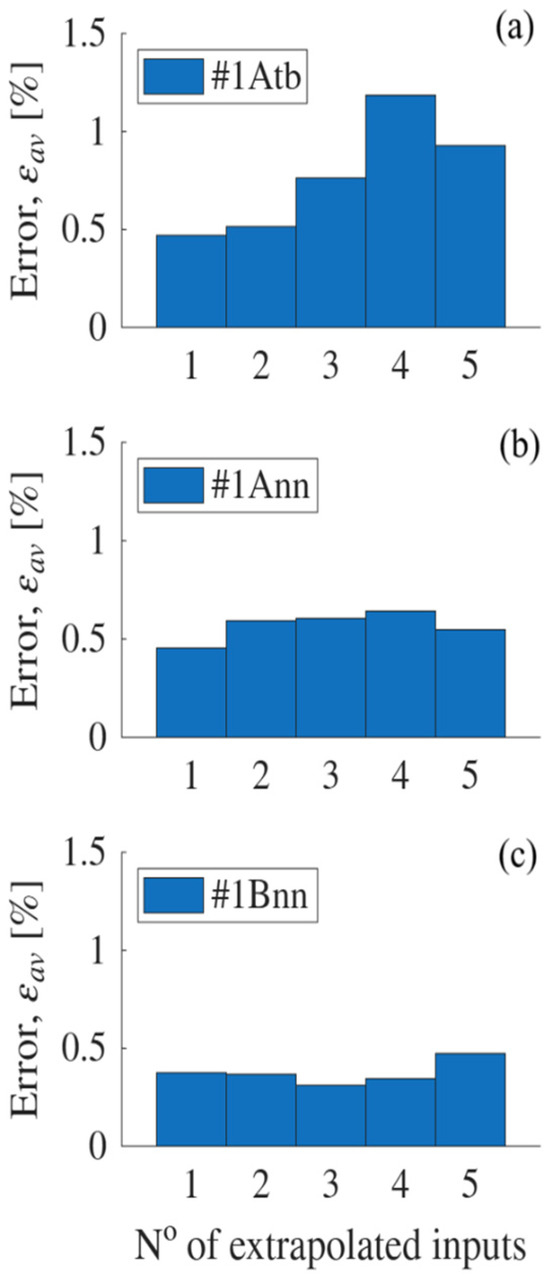
A limited direct problem extrapolation test was performed using 31 additional CFD cases. Each case combined between one and five normalised inputs at 1.05, corresponding to 5% above their upper bounds, while the remaining inputs were fixed at 0.5. As shown in Figure 7, the mean errors remained comparable to those obtained within the original domain: approximately 1% for #1Atb, slightly below 1% for #1Ann, and below 0.5% for #1Bnn.
Figure 7.
Error bars for the extrapolation error (in %) of cases. (a) #1Atb. (b) #1Ann. (c) #1Bnn. The number of extrapolated inputs in the x-axis.
7. Conclusions
The main conclusion of this benchmark is that, broadly speaking, for the application case that was selected (a pulse detonation engine), both the tensor-based and the neural network-based methods chosen for conceptual design purposes performed with comparable efficiencies when the conditions were the same. This should not be a surprise because, in the end, both methods interpolate data, albeit following different approaches. In addition, some differences were introduced in the application conditions of the methods, and the observed differences in the results are described in the following paragraphs.
For the dimensionally balanced cases involving equal numbers of input and output parameters, the benchmark was interpreted through two complementary comparisons. First, HOSVD and NN were compared using the same factorial databases and the same number of samples to assess the effect of the surrogate method. Under these equivalent database conditions, the two implementations showed broadly comparable accuracy, particularly in terms of average errors. Second, the effect of the sampling distribution was assessed by comparing the NN results obtained with factorial and low-discrepancy databases containing the same number of samples. The low-discrepancy databases consistently produced smaller average and maximum errors, particularly for the inverse problem.
The low-discrepancy data organisation consistently yielded lower errors in the present benchmark, suggesting that it may be advantageous when sampling locations can be freely selected. However, its practical suitability depends on the constraints of the database generation process and should therefore be assessed for each particular application. If a conventional factorial approach was chosen, no significant differences were observed between the tensor-based and the neural network-based methods. Regarding the issue of sparse databases, the tendencies observed were the same as in the high-density database. Concerning the test points that were not dimensionally balanced, errors diminished systematically for the overdetermined cases and increased for the underdetermined cases. Furthermore, differences between tensor-based and neural network-based approaches tended to narrow down further.
This study, which was performed, and the conclusions obtained could only be formally applied to the case of a pulse detonation engine. Cases involving other types of propulsion plants would require additional studies. Even in the case of a pulse detonation engine, an open question remains regarding the situation in which local flow variables instead of global performance parameters are generalised. In this case, it is not clear a priori whether one of the methods outperforms the other or, again, they behave similarly. This could be the subject of future work.
Author Contributions
Conceptualisation, A.G.-V., F.S., E.M. and A.V.; methodology, A.G.-V., F.S. and A.V.; software, A.G.-V., F.S. and E.M.; validation, E.M. and A.V.; formal analysis, A.G.-V. and E.M.; investigation, A.G.-V. and A.V.; resources, F.S. and A.V.; data curation, A.G.-V. and F.S.; writing—original draft preparation, F.S. and A.V.; writing—review and editing, A.G.-V. and F.S.; visualisation, A.G.-V.; supervision, F.S., E.M. and A.V.; project administration, F.S. and A.V. All authors have read and agreed to the published version of the manuscript.
Funding
This research received no external funding.
Data Availability Statement
The data that support the findings of this study are available from the corresponding author upon reasonable request.
Conflicts of Interest
The authors declare no conflicts of interest.
Abbreviations
The following abbreviations are used in this manuscript:
| CJ | Chapman–Jouguet |
| PDE | Pulse detonation engine |
| RDE | Rotating detonation engine |
References
- Bogoi, A.; Cuciuc, T.; Cojocea, A.V.; Gall, M.; Porumbel, I.; Hrițcu, C.E. Experimental Pressure Gain Analysis of Pulsed Detonation Engine. Aerospace 2024, 11, 465. [Google Scholar] [CrossRef] [Scilit]
- Goto, K.; Matsuoka, K.; Matsuyama, K.; Kawasaki, A.; Watanabe, H.; Itouyama, N.; Ishihara, K.; Buyakofu, V.; Noda, T.; Kasahara, J.; et al. Space flight demonstration of rotating detonation engine using sounding rocket S-520-31. J. Spacecr. Rockets 2023, 60, 273–285. [Google Scholar] [CrossRef] [Scilit]
- Buyakofu, V.; Matsuoka, K.; Matsuyama, K.; Kawasaki, A.; Watanabe, H.; Itouyama, N.; Goto, K.; Ishihara, K.; Noda, T.; Kasahara, J.; et al. Flight demonstration of pulse detonation engine using sounding rocket S-520-31 in space. J. Spacecr. Rockets 2023, 60, 181–189. [Google Scholar] [CrossRef] [Scilit]
- Jie, L.; Longxi, Z.; Hua, Q.; Zeyang, X.; Xiaoyao, D. Performance investigation of a pulse detonation turbine engine. Proc. Inst. Mech. Eng. G J. Aerosp. Eng. 2016, 230, 350–359. [Google Scholar] [CrossRef] [Scilit]
- Asli, M.; Garan, N.; Neumann, N.; Stathopoulos, P. A robust one-dimensional approach for the performance evaluation of turbines driven by pulsed detonation combustion. Energy Convers. Manag. 2021, 248, 114784. [Google Scholar] [CrossRef] [Scilit]
- Peace, J.T.; Lu, F.K. Performance modeling of pulse detonation engines using the method of characteristics. Aerosp. Sci. Technol. 2019, 88, 51–64. [Google Scholar] [CrossRef] [Scilit]
- Roux, J.A. Parametric cycle analysis of an ideal pulse detonation engine–Supersonic branch. Therm. Sci. Eng. Prog. 2018, 5, 296–302. [Google Scholar] [CrossRef] [Scilit]
- Hua, Q.I.U.; Xiong, C.; Jianling, L.I. A theoretical and 1-D numerical investigation on a valve/valveless air-breathing pulse detonation engine. Chin. J. Aeronaut. 2021, 34, 68–78. [Google Scholar] [CrossRef] [Scilit]
- Luo, S.; Sun, Y.; Song, J.; Liu, J. Performance analysis of a hybrid pulse detonation engine using liquid hydrogen as fuel. Int. J. Hydrogen Energy 2022, 47, 21537–21551. [Google Scholar] [CrossRef] [Scilit]
- Tan, W.; Zheng, L.; Lu, J.; Xiao, Z. Analysis of dynamic operating characteristics of a pulse detonation turbine engine. Aerospace 2022, 9, 550. [Google Scholar] [CrossRef] [Scilit]
- Xiao, Z.; Lu, J.; Zheng, L.; Liu, K. Energy and exergy analysis of pulse detonation combustor and pulse detonation turbine engine cycle. Case Stud. Therm. Eng. 2024, 64, 105426. [Google Scholar] [CrossRef] [Scilit]
- de Leon, L.S.; Sastre, F.; Martin, E.; Velazquez, A. Reduced-Order Model for Performance Simulation and Conceptual Design of Rocket-Type Pulse Detonation Engines. Aerospace 2025, 12, 132. [Google Scholar] [CrossRef] [Scilit]
- Gonzalez-Viana, A.; Sastre, F.; Martin, E.; Velazquez, A. Multi-Objective Optimization of Rocket-Type Pulse Detonation Engine Nozzles. Aerospace 2025, 12, 502. [Google Scholar] [CrossRef] [Scilit]
- Wolff, S.; Schäpel, J.S.; King, R. Application of artificial neural networks for misfiring detection in an annular pulsed detonation combustor mockup. J. Eng. Gas Turbines Power 2017, 139, 041510. [Google Scholar] [CrossRef] [Scilit]
- Johnson, K.B.; Ferguson, D.H.; Tempke, R.S.; Nix, A.C. Application of a convolutional neural network for wave mode identification in a rotating detonation combustor using high-speed imaging. J. Therm. Sci. Eng. Appl. 2021, 13, 061021. [Google Scholar] [CrossRef] [Scilit]
- Johnson, K.B.; Ferguson, D.H.; Nix, A.C. Use of Convolutional Neural Network Image Classification and High-Speed Ion Probe Data Toward Real-Time Detonation Characterization in a Water-Cooled Rotating Detonation Engine. J. Therm. Sci. Eng. Appl. 2023, 15, 061011. [Google Scholar] [CrossRef] [Scilit]
- Koch, J. Data-driven surrogates of rotating detonation engine physics with neural ordinary differential equations and high-speed camera footage. Phys. Fluids 2021, 33, 091703. [Google Scholar] [CrossRef] [Scilit]
- Mendible, A.; Koch, J.; Lange, H.; Brunton, S.L.; Kutz, J.N. Data-driven modeling of rotating detonation waves. Phys. Rev. Fluids 2021, 6, 050507. [Google Scholar] [CrossRef] [Scilit]
- Shen, D.; Sheng, Z.; Zhang, Y.; Rong, G.; Wu, K.; Wang, J. Predicting combustion behaviour in rotating detonation engines using an interpretable deep learning method. Phys. Fluids 2023, 35, 076105. [Google Scholar] [CrossRef] [Scilit]
- Wang, X.; Wen, H.; Hu, T.; Wang, B. Flow-field reconstruction in rotating detonation combustor based on physics-informed neural network. Phys. Fluids 2023, 35, 076109. [Google Scholar] [CrossRef] [Scilit]
- Johnson, K.B.; Ferguson, D.; Nix, A.C. Machine-learning-based rotating detonation engine diagnostics: Evaluation for application in experimental facilities. J. Propuls. Power 2024, 40, 257–270. [Google Scholar] [CrossRef] [Scilit]
- Sobol, I.M. Distribution of points in a cube and approximate evaluation of integrals. USSR Comput. Math. Math. Phys. 1967, 7, 86–112. [Google Scholar] [CrossRef] [Scilit]
- Moreno, A.I.; Jarzabek, A.A.; Perales, J.M.; Vega, J.M. Aerodynamic database reconstruction via gappy high order singular value decomposition. Aerosp. Sci. Technol. 2016, 52, 115–128. [Google Scholar] [CrossRef] [Scilit]
- Sastre, F.; Sanchez de Leon, L.; Martin, E.B.; Velazquez, A. Surrogate data-driven physics-aware model for the conceptual aerodynamic design of rotating detonation engines. Int. J. Numer. Methods Heat Fluid Flow 2025, 35, 3539–3560. [Google Scholar] [CrossRef] [Scilit]
- Stull, D.R.; Prophet, H. JANAF Thermodynamical Tables; US National Bureau of Standards: Washington, DC, USA, 1971.
- McGough, D.A. Detonation Modeling in OpenFOAM Using Adaptive Mesh Refinement. Master’s Thesis, University of Colorado at Boulder, Boulder, CO, USA, 2020. [Google Scholar]
- Towery, C.A.; Smith, K.M.; Shrestha, P.; Hamlington, P.E.; Van Schoor, M. Examination of turbulent flow effects in rotating detonation engines. In Proceedings of the 44th AIAA Fluid Dynamics Conference; American Institute of Aeronautics and Astronautics: Reston, VA, USA, 2014. [Google Scholar]
- Rai, J.; Parajuli, S.; Abbasi, A.; Hashemi, S. Investigation of different chemical kinetics reaction rates and its relevant modelling for h2-o2 combustion. Int. J. Sci. Eng. Res. 2018, 9, 84–90. [Google Scholar]
- Kurganov, A.; Noelle, S.; Petrova, G. Semidiscrete central-upwind schemes for hyperbolic conservation laws and hamilton-jacobi equations. SIAM J. Sci. Comput. 2001, 23, 707–740. [Google Scholar] [CrossRef] [Scilit]
- Schauer, F.; Stutrud, J.; Bradley, R. Detonation initiation studies and performance results for pulsed detonation engine applications. In Proceedings of the 39th Aerospace Sciences Meeting and Exhibit; American Institute of Aeronautics and Astronautics: Reston, VA, USA, 2012. [Google Scholar]
- Ornano, F.; Braun, J.; Saracoglu, B.H.; Paniagua, G. Multi-stage nozzle-shape optimization for pulsed hydrogen–air detonation combustor. Adv. Mech. Eng. 2017, 9, 1687814017690955. [Google Scholar] [CrossRef] [Scilit]
- Owens, Z.C.; Hanson, R.K. Single-cycle unsteady nozzle phenomena in pulse detonation engines. J. Propuls. Power 2007, 23, 325–337. [Google Scholar] [CrossRef] [Scilit]
- Tucker, L.R. Some mathematical notes on three-mode factor analysis. Psychometrika 1966, 31, 279–311. [Google Scholar] [CrossRef] [Scilit] [PubMed]
- De Lathauwer, L.; De Moor, B.; Vandewalle, J. A multilinear singular value decomposition. SIAM J. Matrix Anal. Appl. 2000, 21, 1253–1278. [Google Scholar] [CrossRef] [Scilit]
- de Lathauwer, L.; de Moor, B.; Vandewalle, J. On the best rank-one and rank (R1, R2, RN) approximation of higher order tensors. SIAM J. Matrix Anal. Appl. 2000, 21, 1324–1342. [Google Scholar]
- Byrd, R.H.; Gilbert, J.C.; Nocedal, J. A Trust Region Method Based on Interior Point Techniques for Nonlinear Programming. Math. Program. 2000, 89, 149–185. [Google Scholar] [CrossRef] [Scilit]
- Byrd, R.H.; Hribar, M.E.; Nocedal, J. An Interior Point Algorithm for Large-Scale Nonlinear Programming. SIAM J. Optim. 1999, 9, 877–900. [Google Scholar] [CrossRef] [Scilit]
- Waltz, R.A.; Morales, J.L.; Nocedal, J.; Orban, D. An interior algorithm for nonlinear optimization that combines line search and trust region steps. Math. Program. 2006, 107, 391–408. [Google Scholar] [CrossRef] [Scilit]
- Cao, Q.; Chen, S.; Zheng, Y.; Ding, Y.; Tang, Y.; Huang, Q.; Wang, K.; Xiang, W. Classification and prediction of gas turbine gas path degradation based on deep neural networks. Int. J. Energy Res. 2021, 45, 10513–10526. [Google Scholar] [CrossRef] [Scilit]
- Manatura, K.; Rummith, N.; Chalermsinsuwan, B.; Samsalee, N.; Chen, W.H.; Phookronghin, K.; Wongrerkdee, S. Gas turbine heat rate prediction in combined cycle power plant using artificial neural network. Therm. Sci. Eng. Prog. 2025, 59, 103301. [Google Scholar] [CrossRef] [Scilit]
- Hashmi, M.B.; Mansouri, M.; Fentaye, A.D.; Ahsan, S.; Kyprianidis, K. An artificial neural network-based fault diagnostics approach for hydrogen-fueled micro gas turbines. Energies 2024, 17, 719. [Google Scholar] [CrossRef] [Scilit]
- Raghavan, S.M.; Palatel, A.; Simon, J. Artificial neural networks based parametric curve generation for health assessment of industrial gas turbine systems. Process Integr. Optim. Sustain. 2024, 8, 577–590. [Google Scholar] [CrossRef] [Scilit]
- Talebi, S.S.; Madadi, A.; Tousi, A.M.; Kiaee, M. Micro Gas Turbine fault detection and isolation with a combination of Artificial Neural Network and off-design performance analysis. Eng. Appl. Artif. Intell. 2022, 113, 104900. [Google Scholar] [CrossRef] [Scilit]
- LeCun, Y.; Bottou, L.; Orr, G.B.; Müller, K.R. Efficient backprop. In Neural Networks: Tricks of the Trade; Springer: Berlin/Heidelberg, Germany, 1998; Volume 1524, pp. 9–50. [Google Scholar]
- Glorot, X.; Bengio, Y. Understanding the difficulty of training deep feedforward neural networks. In Proceedings of the Thirteenth International Conference on Artificial Intelligence and Statistics, Sardinia, Italy, 13–15 May 2010. [Google Scholar]
- Kingma, D.P.; Ba, J. ADAM: A method for stochastic optimization. arXiv 2014, arXiv:1412.6980. [Google Scholar]
- Ma, C.; Wu, L.; Weinan, E. A qualitative study of the dynamic behavior for adaptive gradient algorithms. In Mathematical and Scientific Machine Learning; PMLR: Cambridge, MA, USA, 2022; Volume 145, pp. 671–692. [Google Scholar]
- Dababneh, O.; Conway-Smith, J.T. An evaluation of the accuracy of existing empirical and semi-empirical methods for predicting the wing mass of large transport aircraft. Aerospace 2025, 12, 142. [Google Scholar] [CrossRef] [Scilit]
- Niederreiter, H. Random Number Generation and Quasi-Monte Carlo Methods; SIAM: Philadelphia, PA, USA, 1992. [Google Scholar]
- Mishra, S.; Rusch, T.K. Enhancing accuracy of deep learning algorithms by training with low-discrepancy sequences. SIAM J. Numer. Anal. 2021, 59, 1811–1834. [Google Scholar] [CrossRef] [Scilit]

Disclaimer/Publisher’s Note: The statements, opinions and data contained in all publications are solely those of the individual author(s) and contributor(s) and not of MDPI and/or the editor(s). MDPI and/or the editor(s) disclaim responsibility for any injury to people or property resulting from any ideas, methods, instructions or products referred to in the content. |
© 2026 by the authors. Licensee MDPI, Basel, Switzerland. This article is an open access article distributed under the terms and conditions of the Creative Commons Attribution (CC BY) license.