Conceptual Design of Green Propulsive Systems Using Reinforcement Learning

Abstract

Hybrid-electric powertrains offer a solution to significantly reduce aircraft emissions in flight. This study presents a method that couples the generative design of hybrid-electric architectures with reinforcement learning for the optimization of their control parameters. The application proposed is the retrofitting of an ATR-72 with the objective of identifying an optimal green architecture. The results show that a promising candidate is a dual fuel powertrain combining a gas turbine and fuel cells. Compared with a conventional architecture, this concept reduces ${\mathrm{CO}}_2$ and ${\mathrm{NO}}_x$ emissions by up to 74% and 86%, respectively, incurring a payload mass penalty of only 24%.

1. Introduction

As global populations and economies continue to grow, the demand for aviation is projected to increase between 3% and 5% per year by 2050 [1]. However, while air traffic increases, air transport contributes to global warming through the emission of carbon dioxide (${\mathrm{CO}}_2$), nitrogen oxides (${\mathrm{NO}}_x$), water vapor (${\mathrm{H}}_2$O), and the formation of contrails [2]. In 2018, ${\mathrm{CO}}_2$ emissions from aviation were estimated to be 1.59% of global effective radiative forcing (ERF), and ${\mathrm{non-CO}}_2$ aviation emissions were 1.91% [3]. To reduce the aviation industry’s contribution to anthropogenic climate change, the European Union updated its long-term vision in 2022 with the Fly the Green Deal [4]. This roadmap set the ambitious goal of complete climate neutrality by 2050, which requires reducing aircraft emissions significantly. One of the potential solutions identified in the scientific literature lies in the development of hybrid-electric powertrains (HEP) [5,6].

The formal categorizations of HEP architectures proposed by Lorenz et al. [7] and Isikveren et al. [8] served as guidelines for the development of analytical HEP models representing architectures powered by multiple power sources and providing power to multiple propulsive lines. Following this approach, de Vries et al. [9] introduced two hybridization factors to create an analytical model of a generalized HEP powered by two power sources and delivering power to two separate propulsive lines. The two hybridization factors are reported as the supply power ratio, which represents the ratio of power from a single power source to the total generated power, and the shaft power ratio, which represents the ratio of power in a single shaft to the total shaft power. The flexibility and simplicity of this model make it suitable for conceptual design studies, and several design workflows have used it [10]. The original framework proposed by de Vries et al. has since been expanded to include liquid hydrogen as a third energy source [11,12], which can be combusted in a gas turbine [13,14] or converted to electrical power via a fuel cell. In addition to developing conceptual HEP models, recent works have focussed on developing an optimization framework for complex powertrain architectures. Other applications, such as the one proposed by Bussemaker et al. [15], exploited the flexibility of these models in multi-objective optimization frameworks, generating candidate architectures to minimize fuel burn, maximum take-off weight (MTOW), and flight time.

This work proposes an additional step in this direction by combining the generative design of HEP architectures with an optimization framework based on reinforcement learning (RL), similarly to what has been done in the literature for different optimization problems [16,17,18,19]. However, to formulate a reward function for this optimizer, explicit numerical constraints regarding tailpipe emissions are required. This makes the Fly the Green Deal roadmap unsuitable for this specific application, as it relies heavily on system-wide mitigations, such as carbon offsets. Therefore, in this study, the previous EU aviation goals are used, as outlined in Flightpath 2050 [20]. These sustainability goals include a 75% reduction in ${\mathrm{CO}}_2$ per passenger kilometer (pkm), a 90% reduction in ${\mathrm{NO}}_x$ emissions, and a 65% reduction in perceived noise compared to the year 2000 [20]. This method is applied to a retrofit study of the ATR 72-600 according to the design constraints and requirements selected within the European project demoQUAS (https://www.demoquas.eu/ (accessed on 18 August 2026)) and reported in Section 4, while considering technology projections for the year 2050 as the target entry into service. The objective of the project demoQUAS is the creation of a design workflow capable of quantifying input uncertainties and measuring the impact of their propagation on the results. The application selected by the project to demonstrate the impact of uncertainties on the reliability of the results is a retrofit study of the ATR 72-600 as the one considered in this work. To verify the reliability of the results and the effectiveness of the developed design workflow, the retrofit starts by measuring the initial uncertainty due to the discrepancy between the real ATR 72-600 and the one designed as a baseline. However, to measure the impact of input uncertainties without accounting for epistemic uncertainties introduced by design methods, the retrofit study updates the powertrain mass while reducing the payload to keep the MTOW constant. In this work, the same retrofit study is considered for a different reason: reducing the impact of the variables that do not directly depend on the powertrain architecture on the update of the weights of the neural network. Therefore, the proposed application discussed in this work minimizes the payload reduction resulting from the introduction of green enabling technologies and design choices made to adhere to the Flightpath 2050 goals.

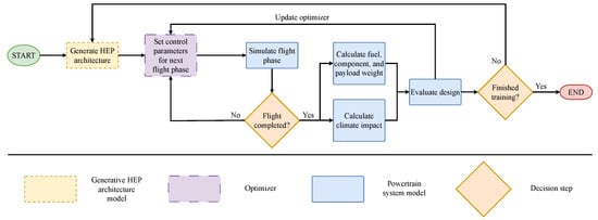
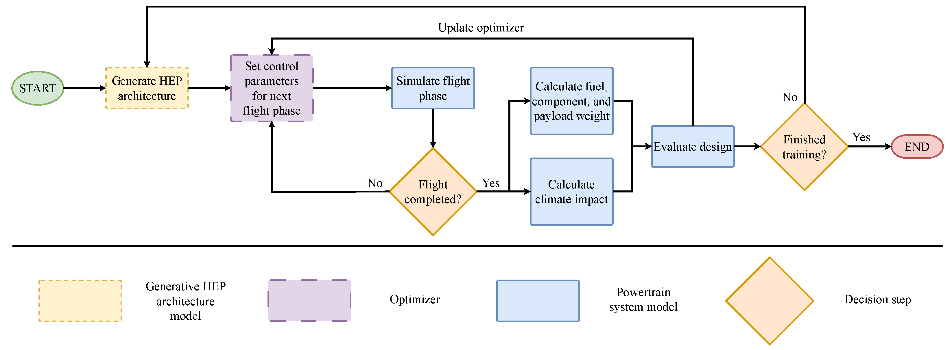
The workflow developed is shown in Figure 1 and further detailed in Section 3. First, a HEP architecture is stochastically generated from the model presented in Section 2 and passed to the optimizer, which sets the control parameters for each flight phase. After a single flight is completed, the weights of systems, fuel, hydrogen, and payload are determined, along with the amount of ${\mathrm{CO}}_2$ and ${\mathrm{NO}}_x$ emitted. Then, the performance is evaluated and used by the optimizer to improve its decision-making by trimming the control parameters. This process is repeated until a specified training threshold is reached, after which the optimizer can determine the optimal control parameters for each HEP architecture. The application of this workflow is introduced in Section 4, where the components’ characteristics are presented. Finally, the results are presented in Section 5.

2. Analytical Models for Design and Analysis of the Powertrain

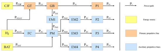
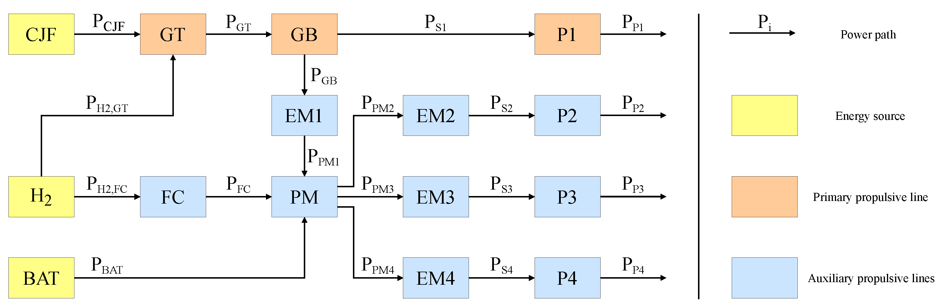
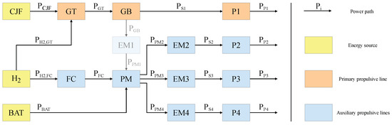
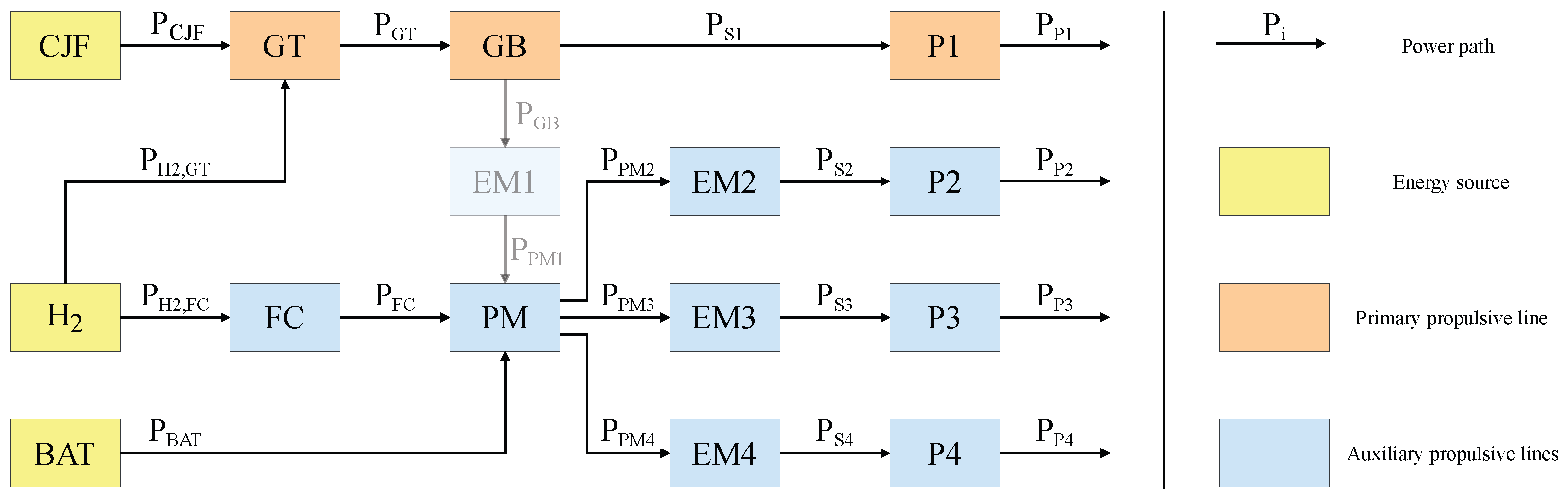
This section introduces the analytical model used to describe the powertrain. The elements considered are clustered into four different groups: power sources, propulsion units, power converters, and power splitters. In this work, three power sources are considered: jet fuel (CJF), liquid hydrogen (${\mathrm{H}}_2$), and battery (BAT). The power converters included in this work are gas turbines (GT), fuel cells (FC), and electric motors (EM). The power management system (PM) and the gearbox (GB) are the two types of power splitter included in this work. Finally, considering the chosen application, namely the ATR 72-600, the propulsion unit considered is the propeller (P). The elements are linked by mechanical or electrical connections, collectively referred to as power paths. Although 28 distinct architectures are presented in the literature [11], this number is based on some assumptions that simplify the computational framework, such as the maximum of two propulsive lines and the connection of each power source to all propulsion lines. However, when assuming that up to three power sources and four independent propulsive lines can be included in a single powertrain architecture, for example, the number of possible architectures increases to 120. The most general representation of this architecture is reported in Figure 2. The remaining 119 architectures are therefore limit cases of this architecture. Concerning the assumptions made in this work, as from other studies from the literature, the symmetry condition is applied to each architecture, whereby the single semi-span configuration reported in Figure 2 is mirrored to represent the aircraft’s full powertrain.

The architecture shown in Figure 2 has a total of 19 different power paths, which are defined as the connection between two elements that exchange power and are represented by arrows in the same figure. Therefore, 19 equations are necessary to solve this system. Using the conservation of energy, Equation (1), a general equation is proposed for the 13 components excluding the energy sources [9].

$${\eta }_{component}·\sum P_{in}=\sum P_{out}$$

(1)

Six equations are formulated as control parameters, which are either the supply or shaft parameters and are bounded within the domain [0,1] [21]. The supply parameters are the ratios between the power delivered by a single energy source and the total power delivered by all energy sources. For a system with N energy sources, there will always be $N-1$ supply parameters. The architecture shown in Figure 2 will therefore have three supply parameters, which are defined by Equations (2)–(4).

$${\mathsf{\Phi }}_{\mathrm{H}2,\mathrm{GT}}={\displaystyle \frac{P_{\mathrm{H}2,\mathrm{GT}}}{P_{\mathrm{CJF}}+P_{\mathrm{H}2,\mathrm{GT}}+P_{\mathrm{H}2,\mathrm{FC}}+P_{\mathrm{BAT}}}}$$

(2)

$${\mathsf{\Phi }}_{\mathrm{H}2,\mathrm{FC}}={\displaystyle \frac{P_{\mathrm{H}2,\mathrm{FC}}}{P_{\mathrm{CJF}}+P_{\mathrm{H}2,\mathrm{GT}}+P_{\mathrm{H}2,\mathrm{FC}}+P_{\mathrm{BAT}}}}$$

(3)

$${\mathsf{\Phi }}_{\mathrm{BAT}}={\displaystyle \frac{P_{\mathrm{BAT}}}{P_{\mathrm{CJF}}+P_{\mathrm{H}2,\mathrm{GT}}+P_{\mathrm{H}2,\mathrm{FC}}+P_{\mathrm{BAT}}}}$$

(4)

The shaft parameters are the ratios between the power delivered by a single shaft and the total shaft power. For the architecture introduced, three shaft parameters are required, which are defined in Equations (5)–(7).

$${\phi }_{\mathrm{S}2}={\displaystyle \frac{P_{\mathrm{S}2}}{P_{\mathrm{S}1}+P_{\mathrm{S}2}+P_{\mathrm{S}3}+P_{\mathrm{S}4}}}$$

(5)

$${\phi }_{\mathrm{S}3}={\displaystyle \frac{P_{\mathrm{S}3}}{P_{\mathrm{S}1}+P_{\mathrm{S}2}+P_{\mathrm{S}3}+P_{\mathrm{S}4}}}$$

(6)

$${\phi }_{\mathrm{S}4}={\displaystyle \frac{P_{\mathrm{S}4}}{P_{\mathrm{S}1}+P_{\mathrm{S}2}+P_{\mathrm{S}3}+P_{\mathrm{S}4}}}$$

(7)

Finally, an additional equation is proposed to close the system of equations by imposing that the total propulsive power required is equal to the sum of the contributions provided by each propulsion element, as in Equation (8) [9].

$$P_p=2·{\displaystyle \sum _{n=1}^{{\mathrm{N}}_{\mathrm{Prop}}}}{P}_{P_n}$$

(8)

Each unique architecture will have a distinct system of equations that depends on the elements present and their connections. Equation (9) is the system of equations associated with the architecture presented in Figure 2, and to solve for each power path, the matrix is inverted and multiplied by the vector on the right-hand side.

$$\left[\begin{array}{ccccccccccccccccccc}-{\eta }_{GT}& 1& 0& 0& -{\eta }_{GT}& 0& 0& 0& 0& 0& 0& 0& 0& 0& 0& 0& 0& 0& 0\\ 0& -{\eta }_{GB}& 1& 0& 0& 0& 0& 0& 0& 1& 0& 0& 0& 0& 0& 0& 0& 0& 0\\ 0& 0& -{\eta }_{P1}& 1& 0& 0& 0& 0& 0& 0& 0& 0& 0& 0& 0& 0& 0& 0& 0\\ 0& 0& 0& 0& 0& 0& 0& 0& 0& -{\eta }_{EM1}& 1& 0& 0& 0& 0& 0& 0& 0& 0\\ 0& 0& 0& 0& 0& 0& 0& 1& 0& 0& 0& -{\eta }_{FC}& 1& 0& 0& 0& 0& 0& 0\\ 0& 0& 0& 0& 0& -{\eta }_{PM}& 1& 0& 0& 0& -{\eta }_{PM}& 0& -{\eta }_{PM}& 1& 0& 0& 1& 0& 0\\ 0& 0& 0& 0& 0& 0& -{\eta }_{EM2}& 1& 0& 0& 0& 0& 0& 0& 0& 0& 0& 0& 0\\ 0& 0& 0& 0& 0& 0& 0& 0& 0& 0& 0& 0& 0& -{\eta }_{EM3}& 1& 0& 0& 0& 0\\ 0& 0& 0& 0& 0& 0& 0& 0& 0& 0& 0& 0& 1& 0& 0& 0& -{\eta }_{EM4}& 1& 0\\ 0& 0& 0& 0& 0& 0& 0& -{\eta }_{P2}& 1& 0& 0& 0& 0& 0& 0& 0& 0& 0& 0\\ 0& 0& 0& 0& 0& 0& 0& 0& 0& 0& 0& 0& 0& 0& -{\eta }_{P3}& 1& 0& 0& 0\\ 0& 0& 0& 0& 0& 0& 0& 0& 0& 0& 0& 0& 0& 0& 0& 0& 0& -{\eta }_{P4}& 1\\ {\mathsf{\Phi }}_{H2,GT}& 0& 0& 0& {\mathsf{\Phi }}_{H2,GT}-1& {\mathsf{\Phi }}_{H2,GT}& 0& 0& 0& 0& 0& {\mathsf{\Phi }}_{H2,GT}& 0& 0& 0& 0& 0& 0& 0\\ {\mathsf{\Phi }}_{BAT}& 0& 0& 0& {\mathsf{\Phi }}_{BAT}& {\mathsf{\Phi }}_{BAT}-1& 0& 0& 0& 0& 0& {\mathsf{\Phi }}_{BAT}& 0& 0& 0& 0& 0& 0& 0\\ {\mathsf{\Phi }}_{H2,FC}& 0& 0& 0& {\mathsf{\Phi }}_{H2,FC}& {\mathsf{\Phi }}_{H2,FC}& 0& 0& 0& 0& 0& {\mathsf{\Phi }}_{H2,FC}-1& 0& 0& 0& 0& 0& 0& 0\\ 0& 0& {\phi }_{S2}& 0& 0& 0& 0& {\phi }_{S2}-1& 0& 0& 0& 0& 0& 0& {\phi }_{S2}& 0& 0& {\phi }_{S2}& 0\\ 0& 0& {\phi }_{S3}& 0& 0& 0& 0& {\phi }_{S3}& 0& 0& 0& 0& 0& 0& {\phi }_{S3}-1& 0& 0& {\phi }_{S3}& 0\\ 0& 0& {\phi }_{S4}& 0& 0& 0& 0& {\phi }_{S4}& 0& 0& 0& 0& 0& 0& {\phi }_{S4}& 0& 0& {\phi }_{S4}-1& 0\\ 0& 0& 0& 1& 0& 0& 0& 0& 1& 0& 0& 0& 0& 0& 0& 1& 0& 0& 1\end{array}\right]·\left[\begin{array}{c}{P}_{CJF}\\ P_{GT}\\ P_{S1}\\ P_{P1}\\ P_{H2,GT}\\ P_{BAT}\\ P_{PM2}\\ P_{S2}\\ P_{P2}\\ P_{GB}\\ P_{PM1}\\ P_{H2,FC}\\ P_{FC}\\ P_{PM3}\\ P_{S3}\\ P_{P3}\\ P_{PM4}\\ P_{S4}\\ P_{P4}\end{array}\right]=\left[\begin{array}{c}0\\ 0\\ 0\\ 0\\ 0\\ 0\\ 0\\ 0\\ 0\\ 0\\ 0\\ 0\\ 0\\ 0\\ 0\\ 0\\ 0\\ 0\\ P_p\end{array}\right]$$

(9)

Although the number of supply parameters is directly related to the number of energy sources, this is not the case for the shaft parameters. In fact, for example, when the element EM1 is removed, as shown in Figure 3, two power paths and the associated equations are canceled. Therefore, Equations (1) and (5) are removed from the system of equations.

The system of equations is solved to determine the sizing power of each component and calculate their weights and volumes. The weights and volumes of the energy sources are calculated by dividing the necessary energy requested to each source by the gravimetric and volumetric energy densities, while the characteristics of the other components are calculated from their respective gravimetric and volumetric power densities, as reported in [22]. For the application presented in this work, the total powertrain mass is added to the aircraft’s operational empty mass, from which the mass of the original propulsion system has already been subtracted. The remaining available mass is then allocated to the payload, while keeping the maximum take-off mass (MTOM) constant. The masses of powertrain and payload are distributed throughout the aircraft to keep the center of gravity (CG) within the stability and controllability margins.

Three constraints are necessary to ensure the consistency of the solutions. First, since both the supply and control parameters express a ratio of a single power path relative to the total supplied or shaft power, the sum of both the supply and shaft parameters cannot exceed one. Secondly, the direction of the power paths must be chosen coherently with the supplied and control parameters. For example, in Figure 2, if ${\mathsf{\Phi }}_{\mathrm{BAT}}>0.5$ and ${\phi }_{\mathrm{S}2}+{\phi }_{\mathrm{S}3}+{\phi }_{\mathrm{S}4}<0.5$, the battery is the main power supplier and the primary shaft delivers most of the propulsive power. Therefore, the power must flow from the power management system to the gearbox, contrary to the direction of the arrows. As a result, the sign of these power paths becomes negative, which may result in singularities [10,11]. To avoid this issue, when the value associated with a power path is negative, its direction is reversed, the system of equations is reconstructed, and the system is solved again. Finally, in this work, the considered operating conditions do not include the harvesting of the propellers.

3. Optimization Framework

Optimizing the distribution of power of a simplified hybrid-electric powertrain requires a control strategy that can be adapted to various architectures and flight conditions. Consequently, an algorithm must find the optimal set of control parameters for each case that maximizes a certain objective. This section discusses the method for solving the problem at hand and presents the chosen algorithm to address it.

3.1. Problem Formulation

The power distribution of a hybrid-electric powertrain represents a complex sequential decision-making problem in which optimal control parameters depend on the specific architecture and the current flight phase. Traditional optimization algorithms, such as Genetic Algorithms, are computationally prohibitive for generative design. Because a total of 120 unique architectures are found, employing these methods would require evaluating hundreds of generations from scratch for every generated architecture. While, Reinforcement learning (RL), a machine learning approach in which an agent learns through trial and error to maximize a specific objective, trains a single generalized policy. Other machine learning paradigms, such as supervised and unsupervised learning, aim to make accurate predictions based on labeled data and to uncover hidden patterns or structures in unlabeled data, respectively. However, in uncharted scenarios, where there is no correct or representative example, reinforcement learning offers a distinct advantage by learning from its interactions and experiences [23]. By standardizing varying topologies using a dynamic System and Action Mask, the trained RL agent can instantaneously set control parameters for any architecture without requiring isolated retraining. Furthermore, while RL requires substantial initial sample data, this computational cost is amortized as generating data is inexpensive and evaluating a new architecture is near-instantaneous. Therefore, exploring RL as an optimization method presents a novel framework that generalizes a policy across the entire architectural design space.

RL problems can be formulated as a Markov decision process (MDP), a mathematical framework where actions (${\mathrm{a}}_t$) influence both immediate rewards and future states (${\mathrm{s}}_t$) [24]. For this application, an architecture is generated stochastically at the beginning of each episode (a flight). Then, for each flight phase (a step), the agent observes the aircraft’s status (the state) and outputs the control parameters (the action) to maximize the cumulative reward. The agent must learn to trade off between payload maximization, fuel usage, and climate impact through direct interaction with the powertrain metamodel. To accommodate varying architectures within a single fixed-size interface, the action and state spaces are structured as follows: The Action Space ($\mathcal{A}$) contains an array of six variables corresponding to the maximum number of supply (3) and shaft (3) parameters. The State Space ($\mathcal{S}$) consists of a vector providing context to the agent on which it can base its decision of choosing the values for the action space, and the State Space contains the following elements:

• System Matrix: A powertrain matrix describing the elements and their connections in a HEP, as shown in Equation (9). The system matrix has a fixed size of (19 × 19) representing the maximum possible system dimensions. For limit cases, the powertrain matrix is embedded in the top-left corner, with the remaining elements padded with zeros.
• System Mask: Also a (19 × 19) matrix that contains the active elements of the system matrix. The elements that contain architectural data are set to 1, while the remaining elements are padded with 0.
• Action Mask: An array of the same size as the maximum number of control parameters (6). However, most architectures will have fewer control parameters, and the agent uses this array to determine which parameters are relevant. The active control parameters for each architecture will contain a one, while the remaining elements are padded with zeros.
• Flight Phase Indicator: An array containing normalized values that contain information regarding the current flight phase, the normalized required power, and the normalized duration of the current flight phase. The first instance is the current flight phase, where 0.2 corresponds to take-off, 0.4 to climb, 0.6 to cruise, 0.8 to descent, and 1 to a completed flight.
• Violation Array: The supply and shaft parameters are both constrained such that the sum of both sets may not exceed one. The agent must learn this constraint from the violation array, which contains the absolute difference between each element of the proposed action and the corresponding element of the scaled action. Giving a small penalty for infeasible actions will discourage the agent from selecting such combinations of control parameters.

3.2. Objective Function

As noise is not considered in this work, the Flightpath 2050 goals include a 75% reduction in ${\mathrm{CO}}_2$ emissions per pkm and a 90% reduction in ${\mathrm{NO}}_x$ emissions relative to the year 2000, based on 2050 technology levels. To account for these goals, the objective function is formulated as presented in Equation (10).

$$r_{\mathrm{unscaled}}=\{\begin{array}{}\mathrm{(10a)}& 10·\frac{m_{\mathrm{payload}}}{m_{\mathrm{payload,\; max}}}\hfill & \mathrm{if}{m}_{\mathrm{payload}}>0,\mathrm{CG\; in\; feasible\; range\; and\; goals\; are\; met}\hfill \mathrm{(10b)}& \Delta {\mathrm{CO}}_2+\Delta {\mathrm{NO}}_x\hfill & \mathrm{if}{m}_{\mathrm{payload}}>0,\mathrm{CG\; in\; feasible\; range\; and\; goals\; are\; not\; met}\hfill \mathrm{(10c)}& -\frac{\left|\mathrm{CG}\right|}{{\mathrm{CG}}_{\mathrm{aft}}}\hfill & \mathrm{if}{m}_{\mathrm{payload}}>0,\mathrm{and\; CG\; outside\; feasible\; range}\hfill \mathrm{(10d)}& m_{\mathrm{payload}}\hfill & \mathrm{if}{m}_{\mathrm{payload}}<0\hfill \end{array}$$

Here, $m_{\mathrm{payload}}$ is the payload mass, $m_{\mathrm{payload},\max }$ the payload achieved with a conventional propulsion system, CG is the location of the center of gravity as a percentage of the mean aerodynamic chord (MAC) of the aircraft with the current HEP design, and $C{G}_{\mathrm{aft}}$ is the aft-most feasible CG location as a percentage of the MAC of the reference aircraft. If the design is feasible and the goals are met the payload mass is divided by the maximum achievable payload mass under 2050 technology projections and multiplied by 10 to ensure it is bounded in the domain [0,10]. If the goals are not met, Equation (10b) is used, where $\Delta {\mathrm{CO}}_2$ and $\Delta {\mathrm{NO}}_x$ are formulated in Equations (11) and (12), respectively. For designs with significant ${\mathrm{CO}}_2$ and ${\mathrm{NO}}_x$ emissions during a flight, these values are negative, but become increasingly positive as emissions decrease. This serves as a constraint on the algorithm, as its reward will be significantly reduced if a design fails to meet the Flightpath 2050 goals.

$$\Delta {\mathrm{CO}}_2=\min ({\displaystyle \frac{{\mathrm{CO}}_{2,2000}}{m_{\mathrm{payload},2000}}}·0.25-{\displaystyle \frac{{\mathrm{CO}}_2\mathrm{emissions}}{m_{\mathrm{payload}}}},0)$$

(11)

$$\Delta {\mathrm{NO}}_x=\min ({\displaystyle \frac{{\mathrm{NO}}_{x,2000}·0.1-{\mathrm{NO}}_x\mathrm{emissions}}{m_{\mathrm{payload}}}},0)$$

(12)

Here, ${\mathrm{CO}}_{2,2000}$, ${\mathrm{NO}}_{x,2000}$, and $m_{\mathrm{payload},2000}$ are the ${\mathrm{CO}}_2$, ${\mathrm{NO}}_x$ emissions and the payload mass calculated for the year 2000 with a conventional powertrain design and assuming a turboprop efficiency of 25%. Furthermore, to ensure that the unscaled reward of each function in Equation (10) remains in its own distinct region, the rewards are scaled with Equation (13).

$$r_{\mathrm{scaled}}=\{\begin{array}{}\mathrm{(13a)}& r_{\mathrm{unscaled}}\hfill & \mathrm{if\; Equation\; (10a)\; used}\hfill \mathrm{(13b)}& (10·\frac{m_{\mathrm{payload}}}{m_{\mathrm{payload,\; max}}}-1)·e^{10·r_{\mathrm{unscaled}}}\hfill & \mathrm{if\; Equation\; (10b)\; used}\hfill \mathrm{(13c)}& r_{\mathrm{unscaled}}\hfill & \mathrm{if\; Equation\; (10c)\; used}\hfill \mathrm{(13d)}& \frac{2}{\pi }·10·\arctan (\frac{r_{\mathrm{unscaled}}-b}{b·1000})-5\hfill & \mathrm{if\; Equation\; (10d)\; used}\hfill \end{array}$$

Here b is the unscaled reward that is awarded to the conventional design with 2030 technology projections. If the design is feasible but the goals are not met, Equation (13b), the reward is scaled through an exponential function. These rewards may be positive for low values of $r_{\mathrm{unscaled}}$, but quickly decrease when the emission goals are further exceeded. Furthermore, to ensure the resulting scaled rewards of each function have distinct regions, 5 is subtracted in Equation (13d). As a result, the rewards from Equations (13a) and (13b) are in the domain [−1,10], Equation (13c) are in the domain [−5,−1], and Equation (13d) are in the domain [−5,−10]. Finally, although the majority of the reward is received at the end of the flight, a small penalty, namely the sum of the elements in the violation array, is applied after each flight phase to encourage the agent to choose feasible actions.

3.3. Reinforcement Learning Algorithm

In the RL algorithm, the agent aims to learn a specific policy $\pi$(${\mathbf{a}}_t$| ${\mathbf{s}}_t$) that helps it choose an action that maximizes cumulative reward. This policy can either learn from data generated by its current decision-making strategy (on-policy) or from data generated by all its past policies (off-policy). While on-policy agents are more stable, they are less sample-efficient than off-policy agents. Furthermore, the policy bases its choice of actions on the value function that estimates future rewards based on the state, the state-value function V(${\mathbf{s}}_t$), or both the state and the action, the action-value function Q(${\mathbf{s}}_t$, ${\mathbf{a}}_t$) [24]. Finally, the two types of RL methods are model-free methods, which rely on trial-and-error learning, and model-based methods, which use a model to predict future rewards and state transitions. Model-based methods are more sample-efficient but typically require more training time and have lower asymptotic performance than model-free methods. Model-free methods are preferred when the model is very complex, while model-based methods are advantageous when the model is easier to learn than the policy or when only limited interactions with the environment are possible [24].

The metamodel described in Section 2 requires, at maximum, six different control parameters, which are continuous values bounded in the domain [0,1]. Because there is no constraint on the number of interactions and higher asymptotic performance is desired, a model-free method is more appropriate for this application, specifically the soft actor-critic (SAC) algorithm [25,26]. This algorithm uses a critic, a state-value function, that evaluates previous actions taken in specific states and the expected reward from the next state. The evaluation is then used to improve the policy, which guides the actor’s future actions. To incorporate large, continuous domains, the critic and actor are modeled as neural networks and trained with stochastic gradient descent [26]. Furthermore, SAC is a soft algorithm that maximizes expected reward while also maximizing entropy, thereby encouraging greater exploration. The balance between expected reward and entropy depends on the entropy coefficient $\alpha$, which had to be set to a specific value in the first version of the SAC algorithm, developed by Haarnoja et al. [25]. However, setting this hyperparameter is not trivial and requires tuning. In the second version, also developed by Haarnoja et al. [26], the algorithm automatically adjusts the coefficient to explore more in uncertain regions but is more deterministic when the optimal action is already clear. Therefore, the second version is used for this application. Although the algorithm is off-policy, it has been demonstrated to be stable and more sample-efficient than other algorithms. When applied to various challenging multi-dimensional continuous control tasks, it consistently outperformed other algorithms such as PPO, DDPG, and TD3, with increasing margins for tasks with more dimensions [26]. Therefore, if the architectures and, thereby, the number of control parameters are expanded in future research, it is expected that SAC will still outperform other algorithms.

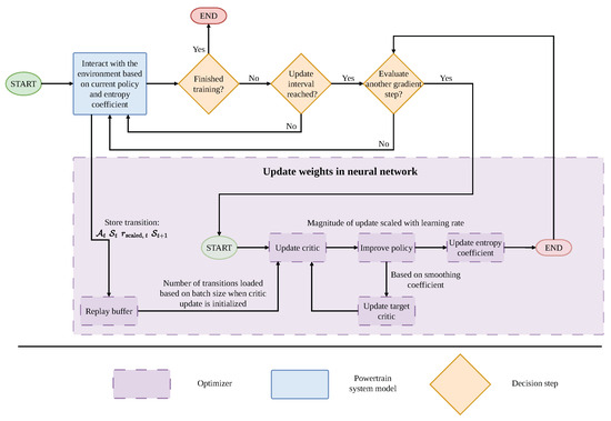
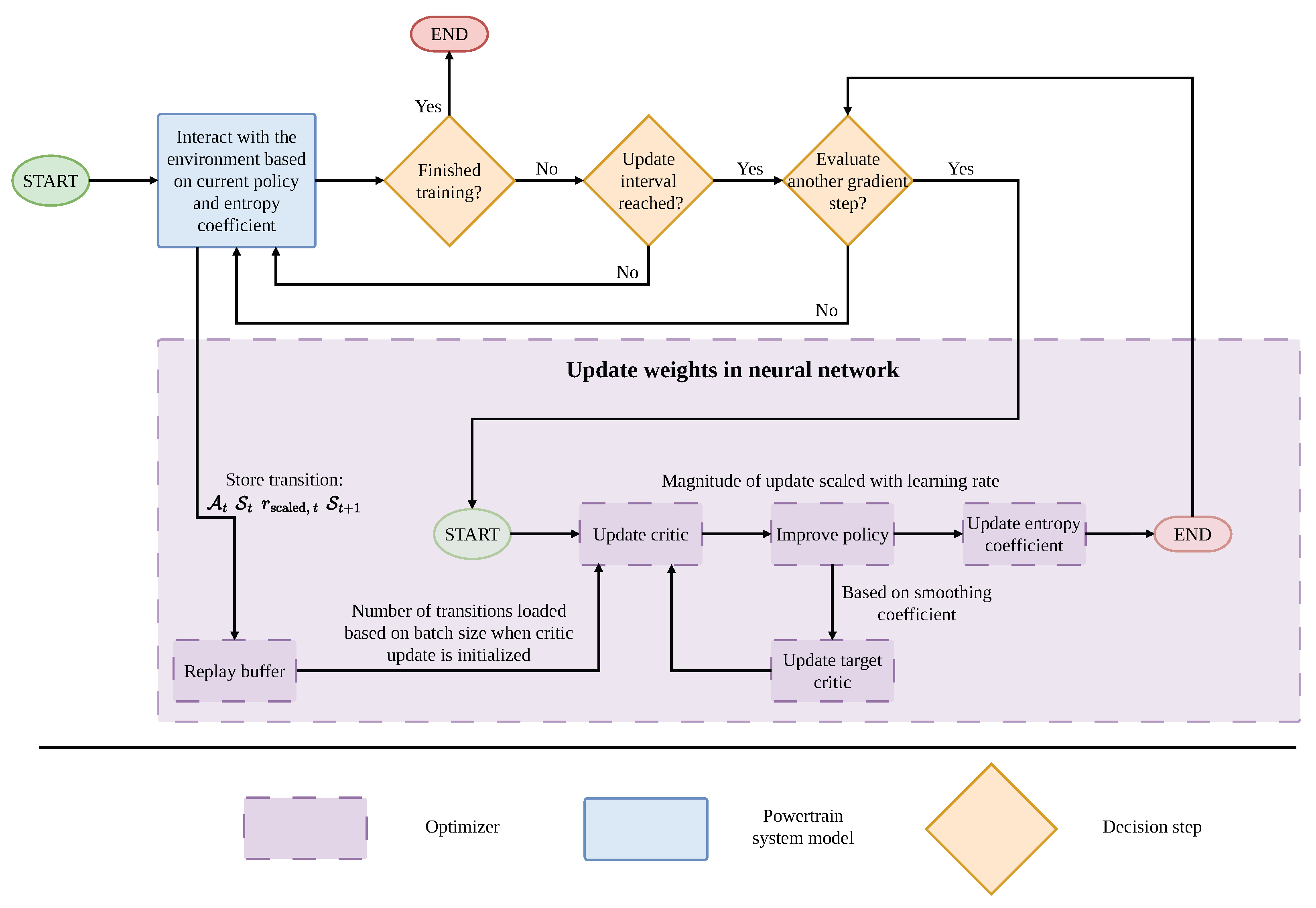
A simplified overview of the SAC algorithm is provided in Figure 4. First 100,000 steps (25,000 flights) are taken without any training to fill the replay buffer. Then, training is initiated, and after a specified interval of steps, n gradient steps are performed, each updating the neural network’s weights n times. Depending on the batch size, a specified number of transitions are sampled from the replay buffer to update the critic. This update is based not only on the expected reward for a given state-action pair but also on the entropy associated with the transition. Then, using the updated critic, the policy is improved, which in turn updates the critic target that is used in the next gradient step. The improved policy also constrains the entropy coefficient, which determines the importance of randomness relative to reward when updating the critic in the next gradient step. This process is repeated for each gradient and training step. Once training is complete, the control parameters are deterministically extracted from the mean of the optimized policy’s probability distribution. The hyperparameters used in this work are similar to those used by Haarnoja et al. [26], except for the ones listed in

Table 1. Description of relevant changed hyperparameters in the SAC algorithm.

Hyperparameter	Description	Default Value	Set Value	Motivation for Set Value
Training frequency	Interval between successive updates. The default is once after every step.	(1, ‘step’)	(1, ‘episode’)	Update once after every episode synchronizes updates with the majority of the reward granted at the end of each episode.
Gradient steps	Number of gradient steps that are taken during each update.	1	16	More gradient steps increases sample efficiency by maximizing learning per environmental interaction.
Buffer size	Capacity of the number of transitions that can be used for sampling.	1,000,000	100,000	Decreased buffer size prioritizes more recent data over ’noisy’ data from exploration.
Batch size	Collected transitions from the replay buffer for each gradient update.	256	2048	Higher sample size increases computational time, but increases stability.
Learning rate	Step size taken by the optimizer to update the network weights.	0.0003	0.0001	Smaller steps result in higher stability and prevents the policy from collapsing.
Smoothing coefficient	Rate of which the target network weights are updated.	0.005	0.01	Higher value accelerates the integration of the policy into the value estimates.

.

3.4. Optimization Verification

While the SAC algorithm does not only aim to maximize its reward, but also entropy by acting as randomly as possible, it does not perform an exhaustive search of the design space. Therefore, the suggested control parameters for each unique architecture are not guaranteed to be global optima. SAC utilizes a stochastic actor to improve stability and exploration in continuous action spaces [26]. However, in design spaces containing steep negative reward gradients near optima, the actor will sample actions near the optima and at the bottom of these gradients. This lowers the expected reward of this region, and the policy may shift to safer areas with higher average returns, potentially moving away from a narrow, sharp optimum.

To identify these narrow, sharp optima and evaluate the performance of the SAC algorithm, the covariance matrix adaptation evolution strategy (CMA-ES) is utilized. This algorithm performs well in black-box continuous optimization problems with non-convex functions [27]. It has been demonstrated to effectively evaluate a large portion of the design space and to outperform other stochastic solvers [28]. CMA-ES optimizes an objective function by stochastically sampling candidate solutions from a multivariate normal distribution. Each sample is evaluated, and the distribution parameters are updated to produce more promising solutions. This process is then repeated for a specific number of generations. The control parameters for each architecture are optimized for 10 and 1000 generations using CMA-ES to verify the SAC algorithm’s results.

4. Case Study: Regional Turboprop Retrofit

The previous two sections discussed a general framework for optimizing the control of hybrid-electric powertrains for a specific objective. This section discusses the chosen reference aircraft to demonstrate the method’s application and the projected characteristics of hybrid-electric powertrain elements for 2050. Furthermore, while a generated architecture can contain up to three auxiliary propulsive lines on a single wing, the effects of distributed propulsion are not considered. Therefore, it is assumed that changing the number of propellers on a wing does not affect the aerodynamic performance. However, previous studies [21] demonstrate that four distributed propellers would remarkably enhance the aerodynamic performance of a regional turboprop, making this hypothesis a minor cause of error. Additionally, because the hybrid-electric architecture is mirrored across both wings, each side will have its own propulsion system independent of the other. Therefore, the certification requirements for one-engine-inoperative conditions, specifically CS 25.147 and CS 25.149 under the CS-25 certification specifications [29], need not be re-evaluated. If the propulsion system of one wing completely fails, the system will still provide adequate power, similar to the one-engine-inoperative condition of the original ATR 72-600. Finally, to ensure passenger safety, the hydrogen storage system cannot be located inside the pressurized cabin; it must be installed either in external pods or within the unpressurized fuselage behind the aft pressure bulkhead. This safety constraint derives from the conclusions reported in the deliverables of the European projects Cocolih2t [30], Cryostar [31], and Concerto [32]. To minimize structural modifications during the retrofit, the storage system is located behind the aft pressure bulkhead.

4.1. Reference Aircraft and Mission

The reference aircraft has a maximum take-off mass of 23,000 kg and can transport 7400 kg of payload, using 2000 kg of CJF, on a nominal mission. Its two engines weigh 1000 kg in total, and the mass of the fuel system is calculated by averaging the methods proposed in the literature [33,34], yielding 57 kg. Subtracting the mass of the engines and the fuel system, the operational empty mass (OEM) calculated net of the propulsion system is equal to 12,543 kg.

Furthermore, the maximum landing weight is 22,350 kg; therefore, at least 650 kg of fuel must be used if the aircraft takes off at maximum weight. However, in hybrid-electric powertrains, gravimetric fuel consumption during nominal flight is lower because the battery mass is nearly constant and hydrogen has a high gravimetric energy density. To ensure a safe landing, three different design considerations may be implemented. First, to account for higher landing loads, the landing gear can be resized, and the resulting mass increase is deducted from the payload mass. Additionally, the landing distance must be re-evaluated, and the increased distance would impose stricter requirements on available landing locations. As this option requires retrofitting beyond the propulsion system and limits the aircraft’s operational envelope, it is not implemented. In fact, while this workflow may be expanded to very complex scenarios including the complete design of the aircraft, the objective of this work was the introduction of an optimization method based on reinforcement learning, and the application focused on the retrofit of the baseline, limiting the modifications to the powertrain. Secondly, a constraint can be implemented, requiring at least 650 kg of fuel to be consumed during a nominal flight. This forces the reinforcement learning algorithm to explore balancing the use of conventional and sustainable fuels and, if successful, verifies its ability to find designs in more complex landscapes. However, applying this constraint will result in designs with higher fuel consumption, favoring less efficient powertrains. Therefore, the final option of limiting the maximum take-off weight by removing payload is implemented, such that the landing weight requirement is not exceeded.

4.1.1. Power Estimation

The normal take-off shaft power of each engine used for the ATR 72-600 is 1846 kW [35]. Assuming a propeller efficiency of 80%, the power output is 2.95 MW. Furthermore, the rate of climb (ROC) is estimated at 1350 feet/min and 300 feet/min at the beginning and top of climb, respectively, while the ROD is constant at 1500 feet/min [36]. The velocity during climb and descent is calculated from the constant indicated airspeed of 170 and 220 kts, and the velocity during cruise is also constant at 270 kts [36]. Finally, the drag coefficient is determined from the ATR 72 drag polar, constructed by Vecchia [37]. The relevant parameters to calculate the required power are reported in

Table 2. Flight phase parameters.

Flight Phase	Mass, kg	$\mathit{\rho }$, ${\mathrm{kg/m}}^3$	V, m/s	${\mathit{C}}_{\mathit{L}}$	${\mathit{C}}_{\mathit{D}}$
Beginning of climb	22,770	1.225	87.46	0.7814	0.05003
Top of climb	22,428	0.5686	128.4	0.7697	0.04944
Cruise	21,638	0.5686	138.9	0.6342	0.04336
Beginning of descent	20,847	0.5686	166.1	0.4272	0.03635
End of descent	20,743	1.225	113.2	0.4251	0.03629

, and the required power itself is listed in

Table 3. Power required and time of each flight phase.

Flight Phase	${\mathit{P}}_{\mathit{p}}$	Time in Phase	${\mathit{P}}_{\mathit{p}}$ Full-Electric Flight
Take-off	2.95 MW	0.5 min	2.95 MW
Climb	2.47 MW	21 min	2.50 MW
Cruise	2.02 MW	146 min	2.09 MW
Descent	0.874 MW	6 min	0.788 MW

.

Based on data from the ATR 72-600 brochure [36], the total flight time for a 740 nm mission is estimated at 173.5 min. By subtracting the estimated durations for the take-off, climb, and descent phases, summarized in Table 3, the remaining time is attributed to cruise.

The fuel fraction method, used to estimate the weight during each phase of flight, accounts for weight reductions due to fuel consumption. However, the weight reduction is smaller when hydrogen or batteries are used as energy sources than with conventional jet fuel. Therefore, the calculated powers in Table 3 may be underestimated during climb and cruise, and overestimated during descent. To quantify the maximum value of this error, while assuming full-electric flight, where the mass remains constant at 23,000 kg, the powers are recalculated and listed in the rightmost column of Table 3. Ultimately, this results in a 3.1% increase in the total energy required. Because this represents the extreme case, full-electric flight without adhering to the maximum landing weight constraint, actual deviations are expected to be smaller across the design space. This suggests that the effect of weight variation, within the bounds of the reference case, on propulsive power is minimal. Therefore, it is assumed that the powers calculated using the fuel fraction method apply to all designs.

4.1.2. Stability and Controllability Verification

To achieve adequate controllability and stability, the centre of gravity (CG) of the aircraft must be within 10% and 39% of the mean aerodynamic chord (MAC) [38].

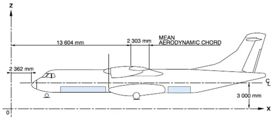
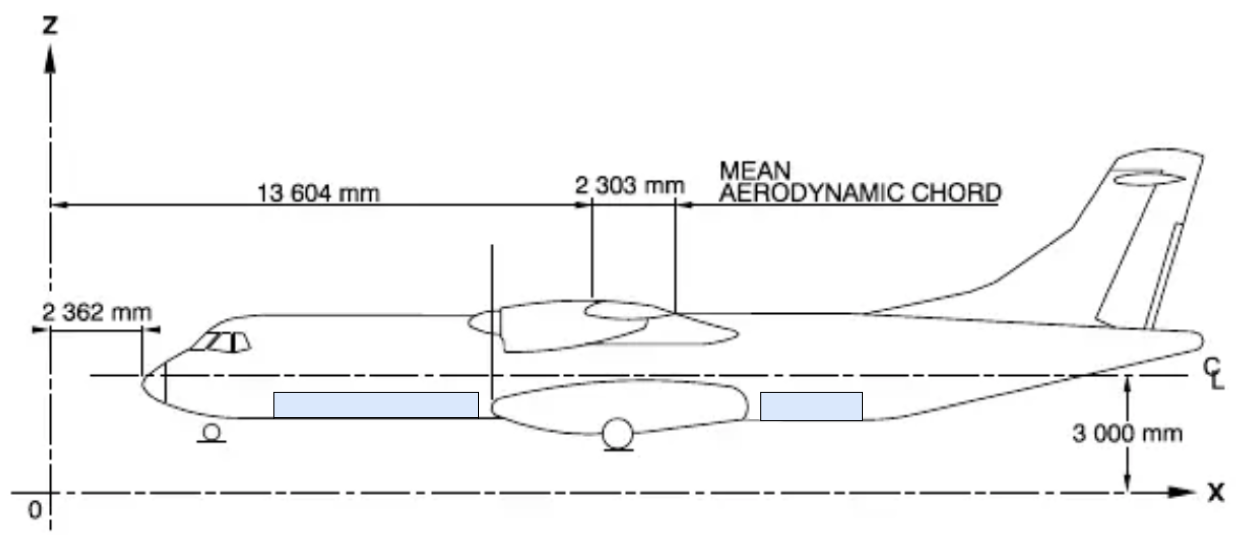
A simplified side view of the aircraft is presented in Figure 5, where the datum line is defined 2.362 m in front of the nose of the aircraft. The fuel, engines, and payload are assumed to be a point mass, and their distances with respect to the datum line are taken from the Weight and Balance manual [38] and reported in

Table 4. Component mass and distance to the datum line of the original ATR 72-600.

Component	Mass, kg	Arm, m
Fuel	2000	14.455
Fuel system	57	14.43
Engines	1000	12.7
Payload	7400	14.755
OEM without propulsion system	12,543	13.91

. Using a value for the center of gravity of 25% of the MAC [38], the arm of the OEM without the propulsion system is calculated.

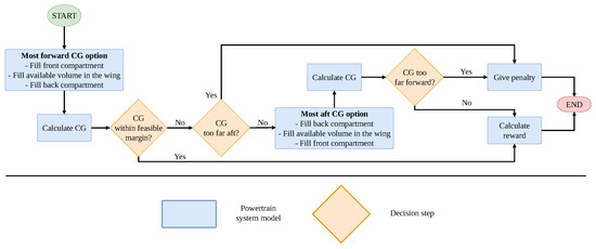
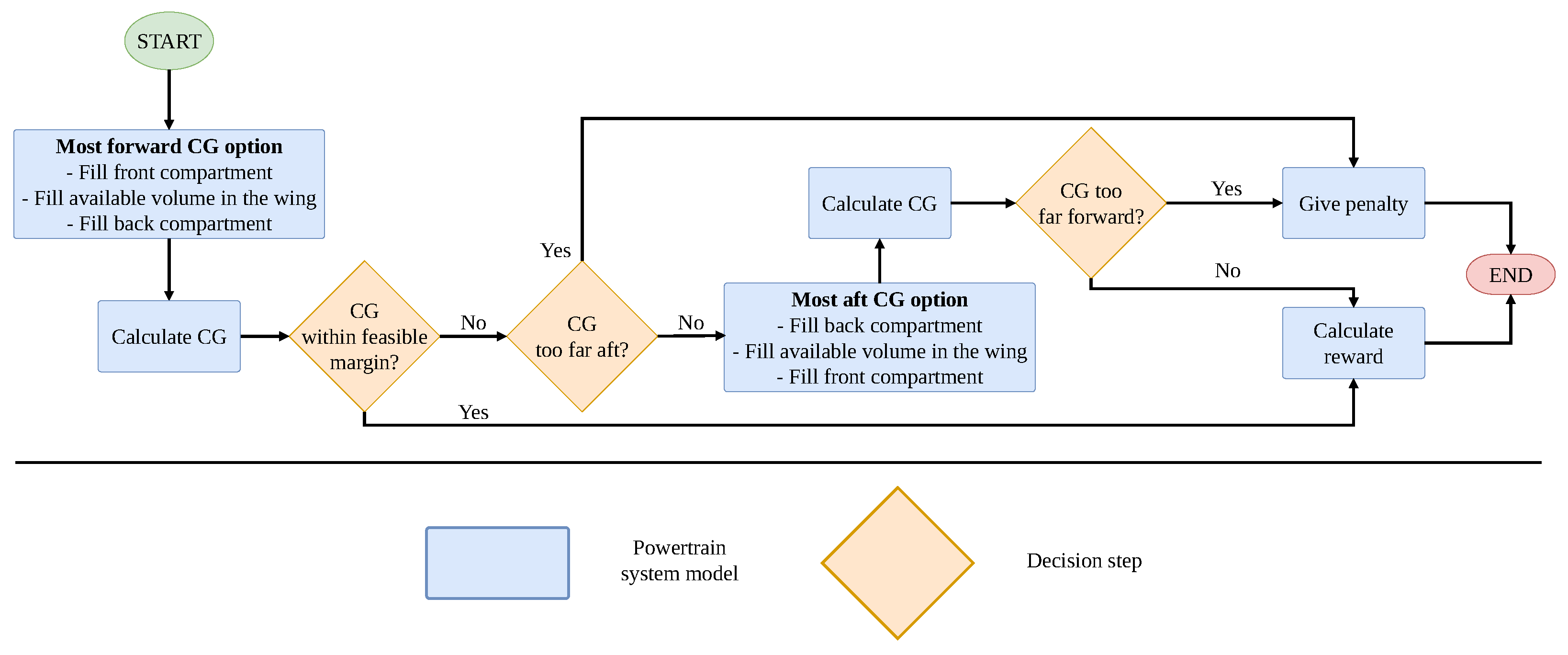
Components such as engines, electric machines, and propellers are all placed on the leading edge (LE) of the wing and will have the same arm as the original engines. Furthermore, CJF and its storage system remain inside the wing, and their CG will move slightly forward depending on the amount of fuel, as reported in the manual [38]. As previously discussed, the hydrogen and its storage system are located behind the aft bulkhead, and the CG is slightly dependent on their respective volumes. The batteries, fuel cells, and power management systems can be stored in the compartments located in front or behind the landing gear, in the shaded regions shown in Figure 5, or in the wing if space is available. In the first iteration, the batteries, fuel cells, and power management system will be loaded from front to back to counter the CG shift caused by the placement of the hydrogen storage system. If this results in the CG being too far forward, the components will be loaded from the rear to the front. The full logic of loading these three types of components is explained in Figure 6. Additionally, due to a potentially heavier propulsion system, passenger capacity may decrease, leaving more cabin space available for passengers. In the front-loading analysis, the passengers are distributed over the cabin with a seat pitch of 29 inches, similar to the original layout. However, in the aft-loading analysis, the seat pitch is increased to distribute passengers along the entire length of the cabin. The range of distances from the mean and the respective locations of each component are listed in

Table 5. Distance to the datum line and location of hybrid-electric aircraft components.

Component or Compartment	Arm, m	Location
OEM without propulsion system	13.91	-
Engines and EM’s	13.1	LE
CFJ and storage system	14.5–14.6	Wing
${\mathrm{H}}_2$ and storage system	20.9–23.7	Aft bulkhead
Payload	8.49–14.8	Fuselage
Front compartment	5.7–11	Fuselage
Wing	14.7	Wing
Back compartment	18–21	Fuselage

, as well as the locations of the compartments used for component storage.

4.1.3. Emissions

The emission index (EI) of ${\mathrm{CO}}_2$ is 3.16 kg/kg, which means that each kg of CJF combusted in the gas turbine emits 3.16 kg of ${\mathrm{CO}}_2$ into the atmosphere. While the EI of ${\mathrm{CO}}_2$ is independent of throttle setting, the EI of ${\mathrm{NO}}_x$ is greatly dependent on this parameter. Therefore, a statistical model developed by Filippone et al. [39] uses the throttle setting and pressure ratio (OPR) of a turboprop and accounts for pressure, temperature, and humidity, as tabulated in Table 6, to estimate the EI of ${\mathrm{NO}}_x$ for each phase of flight. The OPR is assumed to have a constant value of 14 for all flight phases, which is within the range of the PW127 engine suggested by Yuksel et al. [40]. It is found that the EI may reach up to 16.7 g/kg at maximum throttle setting during take-off.

Furthermore, while the Flightpath 2050 goals do not account for contrail-induced warming, persistent contrails rarely form at the typical cruise altitudes of the ATR 72-600 (below 8 km) [41,42,43]. Consequently, contrail effects are excluded from the analysis. Similarly, direct water vapor emissions are neglected, as their contribution to radiative forcing is negligible when emitted in the troposphere [3].

Table 6. Ambient conditions in each flight phase.

Flight Phase	Average Altitude, m	Temperature, K	Pressure, Pa	RH [44]
Take-off	0	288.15	101,325	90%
Climb	3658	264.37	64,437.5	45%
Cruise	7315	240.60	39,272.1	20%
Descent	3658	264.37	64,437.5	45%

Table 6. Ambient conditions in each flight phase.

Flight Phase	Average Altitude, m	Temperature, K	Pressure, Pa	RH [44]
Take-off	0	288.15	101,325	90%
Climb	3658	264.37	64,437.5	45%
Cruise	7315	240.60	39,272.1	20%
Descent	3658	264.37	64,437.5	45%

4.2. Technology Projection Levels

For component sizing, it is necessary to define the energy or power density of each component. In this work, future technology projection levels for 2050 are presented and summarized in

Table 7. Overview of the projected technology levels considered in this work.

	${\mathit{\eta }}_{\mathbf{component}}$	Energy Density	Power Density
CJF Storage	100%	42 MJ/kg|34 MJ/l	-
${\mathrm{H}}_2$ Storage	100%	16 MJ/kg|7.8 MJ/l	-
Batteries	90%	2.2 MJ/kg|3.4 MJ/l	0.73
GT	35%	-	3.77 kW/kg
FC	60%	-	1.4 kW/kg|0.46 kW/l
EM	98%	-	24 kW/kg
PM	99%	-	39 kW/kg|91 kW/l
GB	96%	-	-
Propeller	80%	-	-

.

CJF has a gravimetric and volumetric energy density of 43.2 MJ/kg and 33.91 MJ/l [45], respectively, and it is assumed that these will not increase in the future. When the storage system’s weight is also accounted for, the fuel’s gravimetric density decreases to 42 MJ/kg. Furthermore, the gravimetric energy density of hydrogen itself is 120 MJ/kg; its storage system is of significant weight. For cryogenic-compressed storage, the gravimetric and volumetric energy densities are estimated at 12 MJ/kg and 6 MJ/l [46,47], respectively, for 2030. It is assumed that the volumetric and gravimetric energy densities will increase by 30% in 2050 compared to 2030, reaching 15.6 MJ/kg and 7.8 MJ/l [46]. Furthermore, Tiede et al. [48] predicted, based on historical data and the practical limitations of each battery type, the state-of-the-art gravimetric energy density for 2030, 2040, and 2050 under conservative, nominal, and aggressive technology-advancement rates. The expected gravimetric energy density and efficiency of the nominal case in 2050 are tabulated in Table 7. de Vries et al. [49] assume a charge and discharge rate of 1.2C, meaning the power density, in W/kg, is 1.2 times larger than the energy density, in Wh/kg. The same rate is used in Table 7 to estimate the power density. It is estimated that by 2035, lithium-ion batteries will achieve volumetric energy densities between 600–800 Wh/l, lithium-sulfur batteries between 300–350 Wh/l, and lithium-oxygen batteries between 1000–1600 Wh/l [50]. However, the uncertainty for the latter two is deemed high, whereas that for the lithium-ion type is low. Therefore, an energy density of 600 Wh/l, the conservative side of the 2035 projection, is assumed to be realized by 2030. The ratio between the gravimetric and volumetric energy densities in 2030 is then used to estimate the density in 2050, which is tabulated in Table 7.

The thermal efficiency of the turboprop is estimated to be in the range of 0.25–0.35 [40,51,52]. For this study, it is assumed that efficiency remains at 35% until 2050. For the gas turbine’s continuous power density, a value similar to that of the original ATR 72-600 engines is used [35]. Two types of fuel cells are considered for aviation applications: proton exchange membrane fuel cells (PEMFCs) and solid-oxide fuel cells (SOFCs). However, SOFCs operate most efficiently under steady-state conditions and are therefore not suitable for regional aircraft [22]. For this reason, they are not further considered in this work. Current estimates place power densities of a PEMFC stack at 3.0 kW/kg and 3.4 kW/l [22], which decrease to 1.0–1.5 kW/kg [53] and 0.35 kW/l for the entire system [22]. Therefore, system-level power densities of 1.1 kW/l and 0.35 kW/l, with an efficiency of 55%, are considered reasonable targets for 2030. And it is assumed that power densities will continue to improve by 30% in 2050, while efficiency will only reach its current upper bound of 60% [22]. Furthermore, permanent magnet synchronous machines (PMSMs) are currently the most widely used electric machines in electric and hybrid electric vehicles. They are considered the most attractive option for aviation, due to their high specific power and efficiency [54,55,56]. The expected power densities and efficiencies with a normal confidence level for 2050 are reported in Table 7 [54]. The power management system densities are estimated at 30 kW/kg and 70 kW/l in 2030 [22,57], with an efficiency of 99% [58]. Again, both densities are assumed to increase by 30% in 2050. Finally, de Vries [58] assumes a 96% efficiency for the gearbox, while its weight and that of the propeller are neglected, which has an efficiency of 80% [59].

5. Results

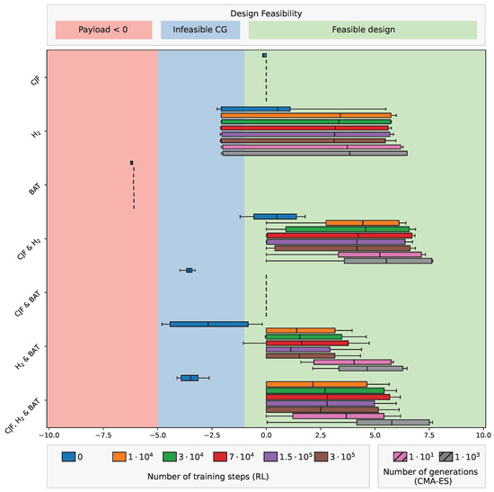
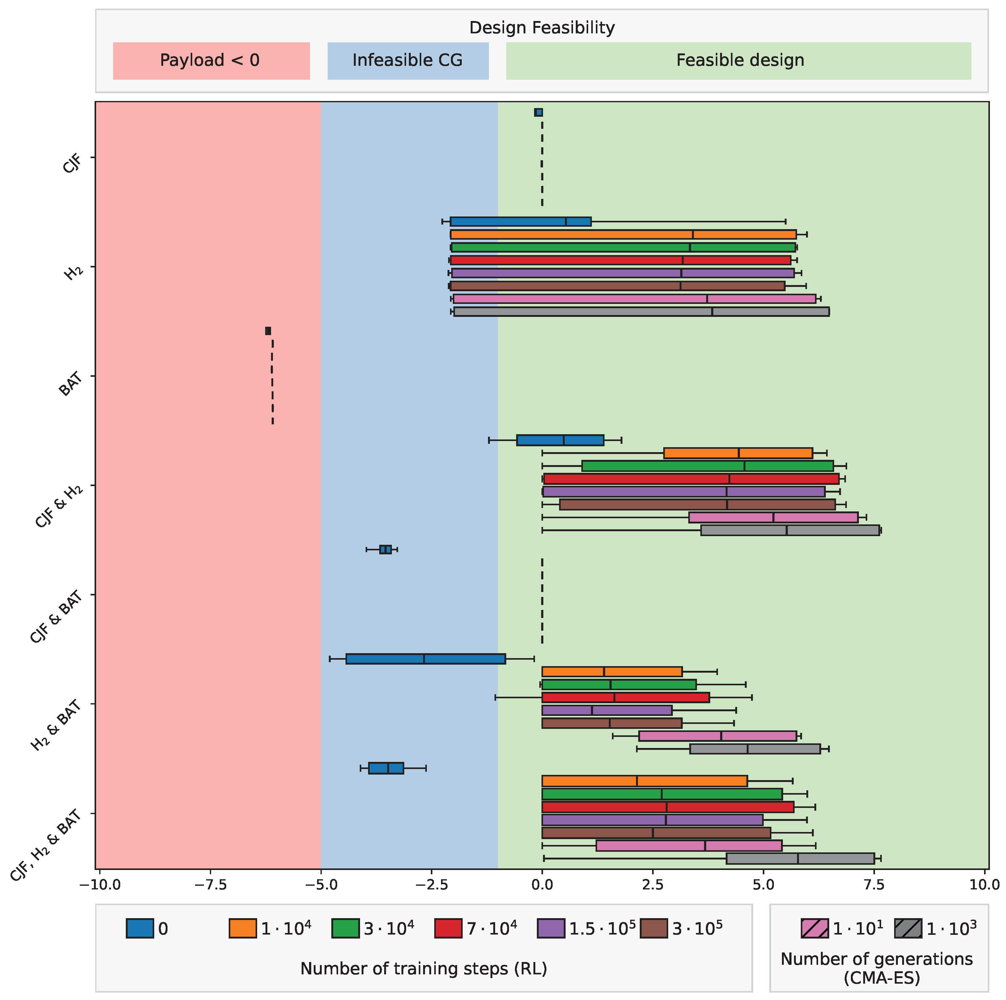
The performance of the RL model is presented in Figure 7, where it can be seen that the scaled reward varies with different combinations of energy sources and the number of training steps. It is observed that model training has been successful as it outperforms random selection of control parameter values (zero training steps) across all architectures. Training the model with more steps results in higher rewards, with the most improvement seen after 10,000 steps, but the returns usually diminish after 70,000 steps. In contrast, when positive rewards are achievable, the CMA-ES algorithm generally outperforms the RL approach after only 10 generations and demonstrates further performance gains after 1000 generations. Furthermore, rewards for architectures containing only CJF remain very close to the baseline. The only possible variations in these architectures are how power is distributed between primary and auxiliary propulsive lines. By omitting the benefits of distributed propulsion in the analysis, it follows that these architectures cannot improve existing designs. Additionally, architectures that contain only batteries are always too heavy as a result of the low gravimetric energy density of these energy sources.

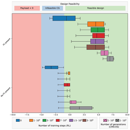
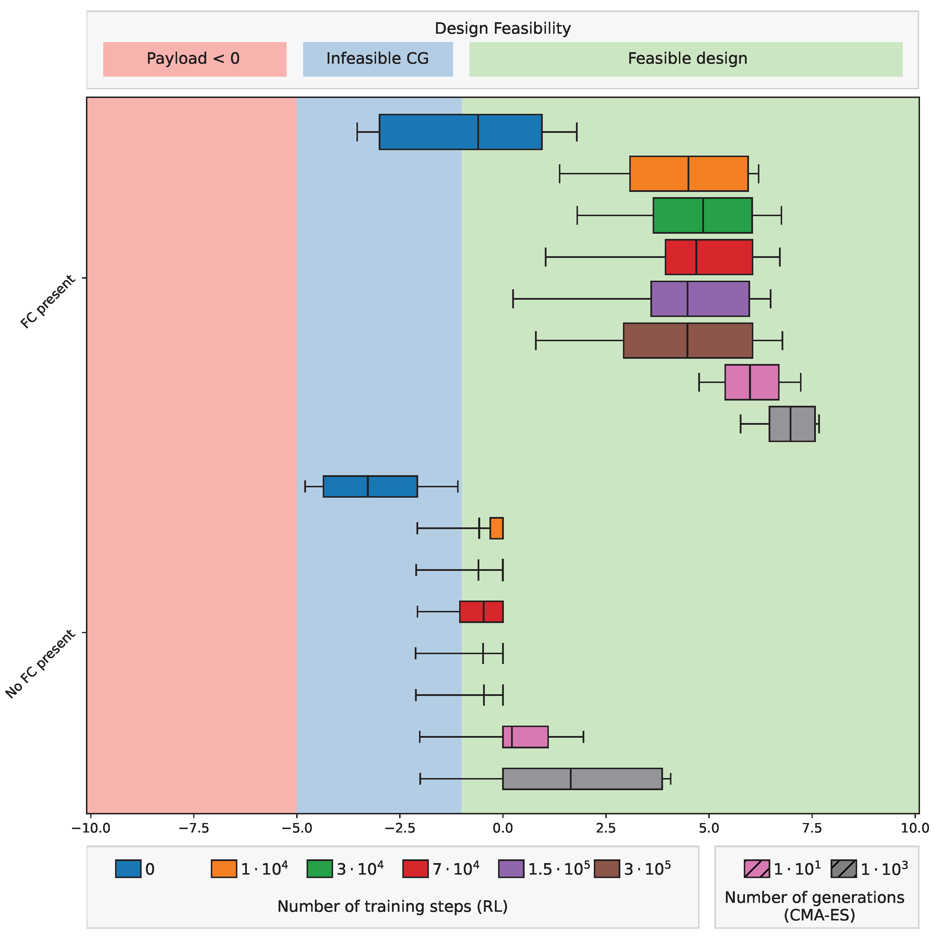
The only improvement compared to the baseline that the model has found is in the architectures where hydrogen is present. Demonstrating the added value of the generative algorithm in identifying other architectures. The highest rewards are found in architectures containing both CJF and hydrogen, while the addition of batteries to these architectures lowers the average reward obtained. A large distribution of rewards for these architectures is also observed. This is the result of using two different methods to convert hydrogen into power: combustion in a gas turbine or its use in fuel cells. Whereas the former has efficiencies between 30–35% and still emits ${\mathrm{NO}}_x$, contributing to global warming, the latter’s efficiency is between 55–60% and completely climate neutral. This effect is shown in Figure 8, where instead of differentiating all the architectures by their energy sources, the presence of a fuel cell now separates the two types of combinations. It is observed that improvements compared to the baseline can only be achieved by using fuel cells. Additionally, hydrogen combustion may lead to infeasible designs. Its lower overall efficiency requires more hydrogen, resulting in a heavier storage system. This shifts the CG too far aft, outside the feasible range. In fact, in line with the assumption of keeping the structural mass constant, both the wing and horizontal tailplane have constant area and position.

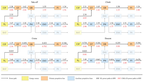
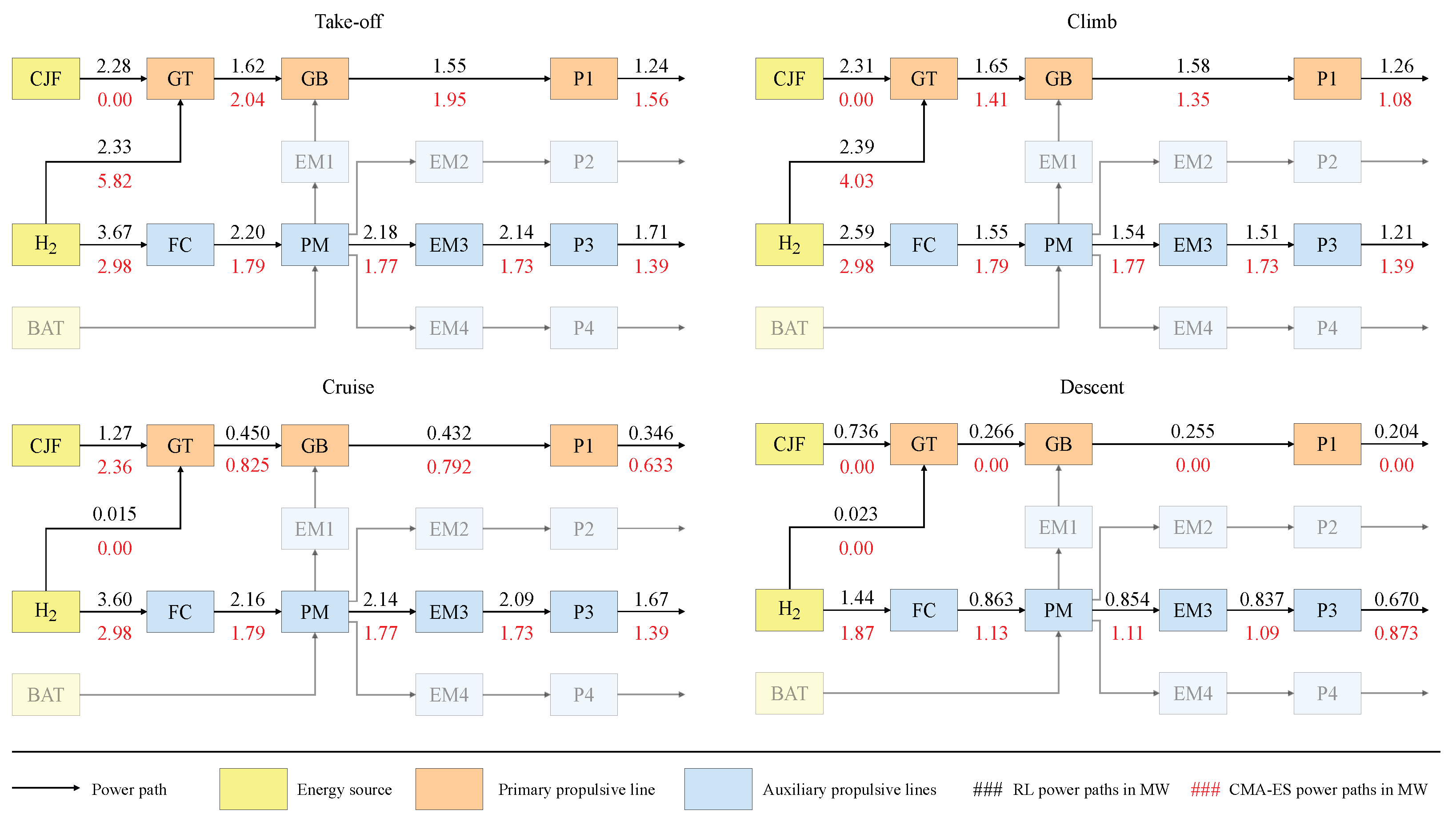
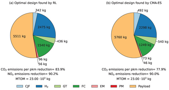
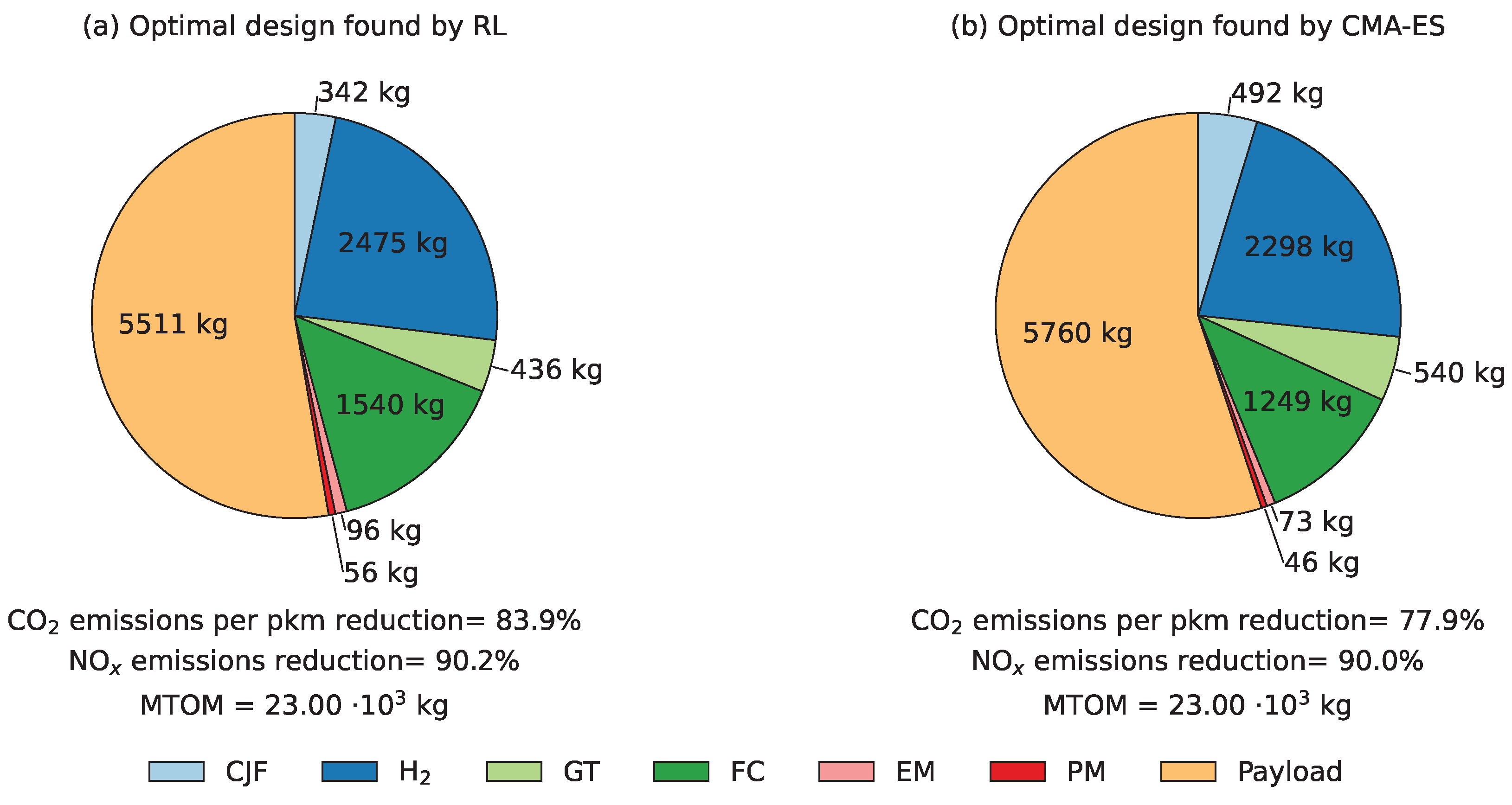
Furthermore, the model identified a single optimal design, and the corresponding architecture, along with the value of each power path for each phase of flight, is shown in black in Figure 9. This shows a control strategy in which the gas turbine is used during phases with high propulsive power requirements, whereas in other phases the relative share of fuel cell output power increases. It is also observed that the power delivered by the fuel cell remains relatively constant, minimizing redundant fuel cell weight during phases when it does not deliver its maximum power. The mass breakdown of this design is shown in Figure 10a, which shows a 25.5% decrease in payload compared to the conventional design. Furthermore, the RL model has exceeded the Flightpath 2050 goals, reducing ${\mathrm{CO}}_2$ emissions per pkm by 83.9% and ${\mathrm{NO}}_x$ emissions by 90.2%, while 75% and 90% reductions would have sufficed. This is likely a result of the agent being punished for overusing CJF, resulting in noncompliance with the Flightpath 2050 goals. Therefore, it has chosen a safe design with limited payload to reduce the risk of heavy penalties.

The design identified by the CMA-ES algorithm, which maximizes payload while meeting the Flightpath 2050 goals, is shown in Figure 10b. This algorithm has achieved higher rewards than the RL model, demonstrating that a further 4.52% increase in payload is possible. This is achieved by maintaining constant fuel cell output power, while the remainder of the required power is supplied by hydrogen combustion during take-off and climb and by CJF combustion during cruise. Because ${\mathrm{NO}}_x$ emissions are lower with hydrogen combustion in a gas turbine than with CJF, hydrogen combustion is beneficial for phases with higher propulsive power requirements. Conversely, an alternative control strategy in which CJF is used during take-off and climb instead of hydrogen, and hydrogen is reallocated to the cruise phase, such that the design is similar to Figure 10b, results in an increase in ${\mathrm{NO}}_x$ emissions and noncompliance with the Flightpath 2050 goals. Optimizing the distribution of power, as shown in red in Figure 9, reduces ${\mathrm{CO}}_2$ emissions per pkm by 77.9% and ${\mathrm{NO}}_x$ emissions by 90%, indicating that the ${\mathrm{NO}}_x$ goal limits further increases in payload.

6. Conclusions and Future Outlooks

This work proposes a generative algorithm for designing hybrid-electric powertrain architectures, coupled with reinforcement learning to optimize the conceptual design of propulsion systems. This method is applied in a retrofit analysis of the ATR 72-600 propulsion system that maximizes payload while meeting the sustainability goals of Flightpath 2050. The results demonstrate that improvements compared to conventional design require the inclusion of hydrogen fuel cells, due to their higher efficiency and lower climate impact compared to hydrogen combustion. However, the optimal architecture identified by the reinforcement learning algorithm is a hybrid system that uses both fuel cells and dual fuel engines, powered by conventional jet fuel and hydrogen. The most energy-efficient operating mode identified uses the fuel cells to deliver the major part of the supplied power. In the proposed design, the payload mass decreases by 27.1% to keep the maximum take-off mass constant, while simultaneously reducing ${\mathrm{CO}}_2$ emissions per pkm by 83.9% and ${\mathrm{NO}}_x$ emissions by 90.2%.

Despite promising results, the computational framework established in this paper does not include a cost analysis. With increasing complexity and lower payload mass, the cost-effectiveness of the solution can be outperformed by conventional architectures in terms of acquisition and operating costs. Literature studies such as [60] demonstrated higher direct operating costs for the hybrid-electric configuration (up to 69.8%) and an increase in ticket prices of about 36%.

This method provides a quick and straightforward propulsion design strategy for hybrid-electric architectures; however, several adjustments can further improve it. First, accounting for variable component efficiencies may yield different optimal solutions. Specifically, during phases when the gas turbine operates in less efficient regions, electrically assisting the primary shaft may prove beneficial. Second, the aerodynamic effects of distributed propulsion are not considered, limiting this study to the benefits associated with different propulsive architectures rather than the impact at the aircraft level. Third, the impact of the auxiliary system is not included in this preliminary study. The impact of the auxiliary systems refers to the increase in drag as a result of the air inlets for the thermal management system, the weight penalties associated with the additional systems with their associated impact on stability and trim, and the power absorbed by the operations of these systems. However, at the conceptual design level, the impact of the auxiliary systems on the overall weights and power requirements can be accounted for by appropriately modifying the efficiencies and specific powers of the main systems they serve, as is usually done when estimating the weight and efficiency of the gas turbine in conventional design methods.

Regarding the optimization framework, the reinforcement learning algorithm struggled to produce optimal designs when solutions approached a feasibility constraint and was outperformed by the CMA-ES algorithm. Therefore, reformulating the objective function or further tuning of the hyperparameters may improve learning. Furthermore, this research could be expanded by including sustainable aviation fuel as an energy source, which would require a full life-cycle analysis of all elements. Finally, analysis of other types of aircraft may provide valuable insights into how mission characteristics affect the optimal architecture and the corresponding control parameters.

References

- Fuel Cells and Hydrogen 2 Joint Undertaking. Hydrogen-Powered Aviation—A Fact-Based Study of Hydrogen Technology, Economics, and Climate Impact by 2050; Tech. Rep.; Publications Office: Luxembourg, 2020. [Google Scholar] [CrossRef]
- Lee, D.S.; Fahey, D.W.; Forster, P.M.; Newton, P.J.; Wit, R.C.N.; Lim, L.L.; Owen, B.; Sausen, R. Aviation and global climate change in the 21st century. Atmos. Environ. 2009, 43, 3520–3537. [Google Scholar] [CrossRef] [Scilit] [PubMed]
- Lee, D.S.; Fahey, D.W.; Skowron, A.; Allen, M.R.; Burkhardt, U.; Chen, Q.; Doherty, S.; Freeman, S.; Forster, P.; Fuglestvedt, J.; et al. The Contribution of Global Aviation to Anthropogenic Climate Forcing for 2000 to 2018. Atmos. Environ. 2021, 244, 117834. [Google Scholar] [CrossRef] [Scilit] [PubMed]
- European Commission, Directorate-General for Research and Innovation. Fly the Green Deal: Europe’s Vision for Sustainable Aviation; Publications Office of the European Union: Luxembourg, 2022. [Google Scholar] [CrossRef]
- Voskuijl, M.; van Bogaert, J.; Rao, A.G. Analysis and Design of Hybrid Electric Regional Turboprop Aircraft. CEAS Aeronaut. J. 2017, 9, 15–25. [Google Scholar] [CrossRef] [Scilit]
- Salem, K.A.; Palaia, G.; Quarta, A.A. Review of Hybrid-Electric Aircraft Technologies and Designs: Critical Analysis and Novel Solutions. Prog. Aerosp. Sci. 2023, 141, 100924. [Google Scholar] [CrossRef] [Scilit]
- Lorenz, L.; Seitz, A.; Kuhn, H.; Sizmann, A. Hybrid Power Trains for Future Mobility. In Proceedings of the Deutscher Luft- und Raumfahrt Kongress (DLRK), Stuttgart, Deutschland, 10–12 September 2013; pp. 1–17. [Google Scholar] [CrossRef] [Scilit]
- Isikveren, A.; Kaiser, S.; Pornet, C.; Vratny, P. Pre-Design Strategies and Sizing Techniques for Dual-Energy Aircraft. Aircr. Eng. Aerosp. Technol. 2014, 86, 525–542. [Google Scholar] [CrossRef] [Scilit]
- de Vries, R.; Brown, M.T.; Vos, R. A Preliminary Sizing Method for Hybrid-Electric Aircraft Including Aero-Propulsive Interaction Effects. In Proceedings of the Aviation Technology, Integration, and Operations Conference, Atlanta, GA, USA, 25–29 June 2018; pp. 1–29. [Google Scholar] [CrossRef] [Scilit]
- Orefice, F. Conceptual Design of Hybrid-Electric Aircraft. Ph.D. Thesis, Università degli Studi di Napoli Federico II, Napoli, Italy, 2022. [Google Scholar] [CrossRef]
- Borgia, A. Double-Hybrid Powertrain Modelling and Integration in the Conceptual Design Method. Master’s Thesis, Politecnico di Torino, Torino, Italy, 2025. [Google Scholar] [CrossRef]
- Grazioso, G.; Stasio, M.D.; Nicolosi, F.; Trepiccione, S. A Mathematical Model for Hybrid-Electric Propulsion System for Regional Propeller-Driven Aircraft. Energy Convers. Manag. X 2025, 26, 100957. [Google Scholar] [CrossRef] [Scilit]
- Link, S.; Dave, K.; de Domenico, F.; Rao, A.G.; Eitelberg, G. Experimental analysis of dual-fuel (CH4/H2) capability in a partially-premixed swirl stabilized combustor. Int. J. Hydrogen Energy 2025, 101, 427–437. [Google Scholar] [CrossRef] [Scilit]
- Dave, K.; Link, S.; de Domenico, F.; Schrijer, F.; Scarano, F.; Rao, A.G. Kerosene-H2 blending effects on flame properties in a multi-fuel combustor. Fuel Commun. 2025, 101, 100–439. [Google Scholar] [CrossRef] [Scilit]
- Bussemaker, J.; Sánchez, R.G.; Fouda, M.; Boggero, L. Function-based Architecture Optimization: An Application to Hybrid-electric Propulsion Systems. Incose Int. Symp. 2023, 33, 251–272. [Google Scholar] [CrossRef] [Scilit]
- Dhawal, T.; Balamurugan, P. Aircraft routing using dynamic programming and reinforcement learning: A customer-centric approach. J. Air Transp. Res. Soc. 2024, 2, 100018. [Google Scholar] [CrossRef] [Scilit]
- Nigam, R.; Choi, J.; Parikh, N.; Li, M.Z.; Tran, H.T. Survey of Inverse Reinforcement Learning in Aviation and Future Outlooks. J. Aerosp. Inf. Syst. 2026, 23, 305–321. [Google Scholar] [CrossRef] [Scilit]
- Wang, Z.; Pan, W.; Li, H.; Wang, X.; Zuo, Q. Review of deep reinforcement learning approaches for conflict resolution in air traffic control. Aerospace 2022, 9, 294. [Google Scholar] [CrossRef] [Scilit]
- Ruan, J.H.; Wang, Z.X.; Chan, F.T.; Patnaik, S.; Tiwari, M.K. A reinforcement learning-based algorithm for the aircraft maintenance routing problem. Expert Syst. Appl. 2021, 169, 114399. [Google Scholar] [CrossRef] [Scilit]
- European Commission; Directorate-General for Research and Innovation; Directorate-General for Mobility and Transport. Flightpath 2050—Europe’s Vision for aviation—Maintaining Global Leadership and Serving Society’s Needs; Publications Office: Luxembourg, 2011. [Google Scholar] [CrossRef]
- Orefice, F.; Della Vecchia, P.; Ciliberti, D.; Nicolosi, F. Aircraft conceptual design including Powertrain System Architecture and distributed propulsion. In Proceedings of the AIAA Propulsion and Energy Forum, Indianapolis, IN, USA, 19–22 August 2019; pp. 1–20. [Google Scholar] [CrossRef] [Scilit]
- Ciliberti, D.; Vecchia, P.D.; Memmolo, V.; Nicolosi, F.; Wortmann, G.; Ricci, F. The Enabling Technologies for a Quasi-Zero Emissions Commuter Aircraft. Aerospace 2022, 9, 319. [Google Scholar] [CrossRef] [Scilit]
- Kaelbling, L.P.; Littman, M.L.; Moore, A.W. Reinforcement learning: A survey. J. Artif. Intell. Res. 1996, 4, 237–285. [Google Scholar] [CrossRef] [Scilit]
- Lonza, A. Reinforcement Learning Algorithms with Python; Packt Publishing: Brimingham, UK, 2019; ISBN 9781789139709. [Google Scholar]
- Haarnoja, T.; Zhou, A.; Abbeel, P.; Levine, S. Soft Actor-Critic: Off-Policy Maximum Entropy Deep Reinforcement Learning with a Stochastic Actor. arXiv 2018, arXiv:1801.01290. [Google Scholar] [CrossRef] [Scilit]
- Haarnoja, T.; Zhou, A.; Hartikainen, K.; Tucker, G.; Ha, S.; Tan, J.; Kumar, V.; Zhu, H.; Gupta, A.; Abbeel, P.; et al. Soft Actor-Critic Algorithms and Applications. arXiv 2019, arXiv:1812.05905. [Google Scholar] [CrossRef] [Scilit]
- Nomura, M.; Shibata, M. CMAES: A Simple yet Practical Python Library for CMA-ES. arXiv 2024, arXiv:2402.01373. [Google Scholar] [CrossRef] [Scilit]
- Rios, L.M.; Sahinidis, N.V. Derivative-Free Optimization: A Review of Algorithms and Comparison of Software Implementations. J. Glob. Optim. 2012, 56, 1247–1293. [Google Scholar] [CrossRef] [Scilit]
- European Union Aviation Safety Agency (EASA). Certification Specifications and Acceptable Means of Compliance for Large Aeroplanes (CS-25), Amendment 28; Tech. Rep. ED Decision 2023/021/R; European Union Aviation Safety Agency: Cologne, Germany, 2023; Available online: https://www.easa.europa.eu/en/downloads/139073/en (accessed on 4 August 2026).
- Simonetto, M.; Pascoe, J.; Sharpanskykh, A. Preliminary Safety Assessment of a Liquid Hydrogen Storage System for Commercial Aviation. Safety 2025, 11, 27. [Google Scholar] [CrossRef] [Scilit]
- European Commission. Certification Roadmap to Yield an Optimal and Safety Methodology of Crashworthiness for an Integrated Cryogenic Tank for Liquid Hydrogen Storage on Board of Future Aircraft; Project Fact Sheet; European Commission: Luxembourg, 2025. [Google Scholar] [CrossRef] [Scilit]
- Jezegou, J.; Almeida-Marino, M.; Horvat, A.B.; Jimenez Carrasco, B.; Last, J.; Leleu, C.; Loison, R.; O’Sullivan, G.; Rene-Corail, M. D3.10-H2 PoC: Analysis of Regulations in Force, Risks and Gaps; Document No. CONCERTO-DEL D-3.2.3-1, Issue 2; CONCERTO Consortium: Brussels, Belgium, 2025; Available online: https://www.concertoproject.eu/public-deliverables (accessed on 12 August 2026).
- Raymer, D.P. Aircraft Design: A Conceptual Approach, 6th ed.; American Institute of Aeronautics and Astronautics: Reston, VA, USA, 2018; ISBN 978-1624107153. [Google Scholar]
- Torenbeek, E. Synthesis of Subsonic Airplane Design; Springer: Dordrecht, The Netherlands, 1982. [Google Scholar] [CrossRef] [Scilit]
- European Union Aviation Safety Agency. Type Certificate Data Sheet No. IM.E.041—PW100 Series Engines; Tech. Rep.; EASA: Cologne, Germany, 2023; Available online: https://www.easa.europa.eu/en/downloads/7725/en (accessed on 4 August 2026).
- Orefice, F.; Corcione, S.; Nicolosi, F.; Ciliberti, D.; Rosa, G.D. Performance calculation for hybrid-electric aircraft integrating aero-propulsive interactions. In Proceedings of the AIAA Scitech Forum, Virtual Event, 11–15 & 19–21 January 2021. [Google Scholar] [CrossRef] [Scilit]
- Vecchia, P.D. Development of Methodologies for the Aerodynamic Design and Optimization of New Regional Turboprop Aircraft. Ph.D. Thesis, Università degli Studi di Napoli Federico II, Napoli, Italy, 2013. [Google Scholar]
- Habermann, A.L. Effects of distributed propulsion on wing mass in aircraft conceptual design. In Proceedings of the AIAA Aviation 2020 Forum, Virtual Event, 15–19 June 2020. [Google Scholar] [CrossRef] [Scilit]
- Filippone, A.; Bojdo, N. Statistical Model for Gas Turbine Engines Exhaust Emissions. Transp. Res. Part Transp. Environ. 2018, 59, 451–463. [Google Scholar] [CrossRef] [Scilit]
- Yuksel, O.; Aygün, H. Comparative Performance Analysis of a Turboprop Engine Used in Regional Aircraft by Considering Design and Flight Conditions. Aircr. Eng. Aerosp. Technol. 2025, 97, 345–355. [Google Scholar] [CrossRef] [Scilit]
- Megill, L.; Grewe, V. Investigating the limiting aircraft-design-dependent and environmental factors of persistent contrail formation. Atmos. Chem. Phys. 2025, 25, 4131–4149. [Google Scholar] [CrossRef] [Scilit]
- Schumann, U. Formation, Properties and Climatic Effects of Contrails. Comptes Rendus Phys. 2005, 6, 549–565. [Google Scholar] [CrossRef] [Scilit]
- Park, J. Altitudinal Trends on Seasonal and Geographic Contrail Persistent Regions Over CONUS. In Proceedings of the AIAA Aviation 2025 Forum, Las Vegas, NV, USA, 21–25 July 2025. [Google Scholar] [CrossRef] [Scilit]
- Enteria, N.; Santamouris, M.; Eicker, U. Urban Heat Island (UHI) Mitigation; Springer: Singapore, 2021. [Google Scholar] [CrossRef] [Scilit]
- Edwards, T. “Kerosene” Fuels for Aerospace Propulsion—Composition and Properties. In Proceedings of the 38th AIAA/ASME/SAE/ASEE Joint Propulsion Conference & Exhibit, Indianapolis, IN, USA, 7–10 July 2002; pp. 1–11. [Google Scholar] [CrossRef] [Scilit]
- Massaro, M.C.; Biga, R.; Kolisnichenko, A.; Marocco, P.; Monteverde, A.H.A.; Santarelli, M. Potential and Technical Challenges of on-Board Hydrogen Storage Technologies Coupled with Fuel Cell Systems for Aircraft Electrification. J. Power Sources 2023, 555, 232397. [Google Scholar] [CrossRef] [Scilit]
- Baroutaji, A.; Wilberforce, T.; Ramadan, M.; Olabi, A.G. Comprehensive Investigation on Hydrogen and Fuel Cell Technology in the Aviation and Aerospace Sectors. Renew. Sustain. Energy Rev. 2019, 106, 31–40. [Google Scholar] [CrossRef] [Scilit]
- Tiede, B.; O’Meara, C.; Jansen, R. Battery Key Performance Projections based on Historical Trends and Chemistries. In Proceedings of the 2022 IEEE Transportation Electrification Conference & Expo (ITEC), Anaheim, CA, USA, 15–17 June 2022; pp. 754–759. [Google Scholar] [CrossRef] [Scilit]
- de Vries, R.; Wolleswinkel, R.E.; Jacobson, D.R.; Bonnema, M.; Thiede, S. Battery Performance metrics for large electric passenger aircraft. In Proceedings of the 34th Congress of the International Council of the Aeronautical Sciences, Florence, Italy, 9–13 September 2024; pp. 1–15. Available online: https://www.icas.org/icas_archive/icas2024/data/preview/icas2024_0636.htm (accessed on 4 August 2026).
- Zamboni, J.; Vos, R.; Emeneth, M.; Schneegans, A. A method for the conceptual design of hybrid electric aircraft. In Proceedings of the AIAA Scitech 2019 Forumy, San Diego, CA, USA, 7–11 January 2019. [Google Scholar] [CrossRef] [Scilit]
- National Academies of Sciences, Engineering, and Medicine. Commercial Aircraft Propulsion and Energy Systems Research: Reducing Global Carbon Emissions; The National Academies Press: Washington, DC, USA, 2016. [Google Scholar] [CrossRef] [Scilit]
- Dinc, A.; Gharbia, Y. Energy Analysis of a Turboprop Engine at Different Flight Altitude and Speeds Using Novel Consideration. Int. J. Turbo-Jet 2022, 39, 599–604. [Google Scholar] [CrossRef] [Scilit]
- Datta, A. PEM Fuel Cell MODEL for Conceptual Design of Hydrogen eVTOL Aircraft; Tech. Rep. NASA/CR-20210000284; NASA: Washington, DC, USA, 2021.
- Pastra, C.L.; Hall, C.; Cinar, G.; Gladin, J.; Mavris, D.N. Specific Power and Efficiency Projections of Electric Machines and Circuit Protection Exploration for Aircraft Applications. In Proceedings of the 2022 IEEE Transportation Electrification Conference and Expo (ITEC), Anaheim, CA, USA, 15–17 June 2022; pp. 766–771. [Google Scholar] [CrossRef] [Scilit]
- Lin, H.; Guo, H.; Qian, H. Design of High-Performance Permanent Magnet Synchronous Motor for Electric Aircraft Propulsion. In Proceedings of the 21st International Conference on Electrical Machines and Systems (ICEMS), Jeju, Republic of Korea, 7–10 October 2018; pp. 174–179. [Google Scholar] [CrossRef] [Scilit]
- Andersen, H.; Chen, Y.; Qasim, M.M.; Amato, M.; Cuadrado, D.G.; Otten, D.M.; Greitzer, E.M.; Perreault, D.J.; Kirtley, J.L.; Lang, J.H.; et al. Design and Manufacturing of a High-Specific-Power Electric Machine for Aircraft Propulsion. In Proceedings of the AIAA AVIATION 2023 Forum, San Diego, CA, USA, 12–16 June 2023; pp. 1–17. [Google Scholar] [CrossRef] [Scilit]
- Yamaguchi, K.; Katsura, K.; Yamada, T.; Sato, Y. High Power Density SiC-Based Inverter with a Power Density of 70 kW Liter or 50 kW Kg. IEEJ J. Ind. Appl. 2019, 8, 694–703. [Google Scholar] [CrossRef] [Scilit]
- de Vries, R. Hybrid-Electric Aircraft with Over-the-Wing Distributed Propulsion: Aerodynamic Performance and Conceptual Design. Ph.D. Thesis, Delft University of Technology, Delft, The Netherlands, 2022. [Google Scholar] [CrossRef]
- Gudmundsson, S. General Aviation Aircraft Design, 2nd ed.; Elsevier: Amsterdam, The Netherlands, 2022; ISBN 9780128184653. [Google Scholar]
- Marciello, V.; Cusati, V.; Nicolosi, F.; Saavedra-Rubio, K.; Pierrat, E.; Thonemann, N.; Laurent, A. Evaluating the economic landscape of hybrid-electric regional aircraft: A cost analysis across three time horizons. Energy Convers. Manag. 2024, 312, 118517. [Google Scholar] [CrossRef] [Scilit]
Disclaimer/Publisher’s Note: The statements, opinions and data contained in all publications are solely those of the individual author(s) and contributor(s) and not of MDPI and/or the editor(s). MDPI and/or the editor(s) disclaim responsibility for any injury to people or property resulting from any ideas, methods, instructions or products referred to in the content. |
© 2026 by the authors. Licensee MDPI, Basel, Switzerland. This article is an open access article distributed under the terms and conditions of the Creative Commons Attribution (CC BY) license.