Explicit Modeling Method for Lift Coefficient of High-Speed Vehicle Based on Symbolic Regression

Abstract

Rapid prediction of vehicle lift coefficient is an important issue in aerodynamic design. Traditional CFD/DSMC methods have high computational costs. Although commonly used machine-learning surrogate models offer high prediction efficiency, they struggle to provide explicit mathematical expressions. To balance prediction accuracy and model interpretability, this paper introduces the symbolic regression method and establishes an explicit modeling process for the lift coefficient. Using Mach number, angle of attack, and related flow parameters as inputs, validation is conducted on two-dimensional blunt body DSMC data and three-dimensional missile aerodynamic data, with comparisons against linear regression, quadratic polynomial regression, Kriging, random forest, XGBoost, and multilayer perceptron. The results show that symbolic regression can obtain high-precision explicit expressions on the two-dimensional blunt body data and can also build analytical models with certain predictive capability on the three-dimensional missile data with limited samples. Compared with traditional explicit regression methods, symbolic regression does not require a pre-specified fixed functional form; compared with black-box models, its advantage lies in providing interpretable and editable algebraic expressions. The findings indicate that symbolic regression has application potential in rapid explicit modeling of the lift coefficient.

1. Introduction

Lift and drag coefficients are two fundamental aerodynamic parameters for evaluating the aerodynamic performance of high-speed vehicles. The lift coefficient is closely related to force balance, trajectory control, and maneuverability, whereas the drag coefficient characterizes aerodynamic resistance and directly affects the overall aerodynamic efficiency of the vehicle. In this study, we focus on the rapid and explicit modeling of the lift coefficient. Wind tunnel tests require much time and cost. In addition, support-related tare and interference as well as tunnel wall effects are recognized sources of measurement uncertainty. These effects have been extensively studied, and their evaluation and correction generally require appropriate calibration and case-specific treatment in wind tunnel testing [1,2]. In rarefied gas flows, the continuum assumption fails, and CFD methods based on the Navier–Stokes equations become less applicable. Direct simulation Monte Carlo (DSMC) can simulate transitional rarefied flows, but its computational cost is high [3]. For morphing aircraft with folding wings, traditional CFD requires complex geometry reconstruction and mesh generation, which limits its use in real-time control [4]. High-fidelity simulations for fluid–thermal–structural coupling in high-speed vehicles can take hours or days, and this cost restricts design iteration [5]. These limitations motivate fast and accurate aerodynamic prediction methods [6,7].

Machine-learning methods have shown strong potential in aerodynamic modeling. Their ability to learn complex nonlinear relationships directly from aerodynamic data enables rapid prediction without repeatedly performing expensive high-fidelity simulations. Once trained, these models can provide aerodynamic responses with substantially reduced computational cost, making them attractive for design optimization, parameter studies, and real-time aerodynamic prediction. Researchers applied convolutional neural networks, graph neural networks, and point-cloud networks to learn nonlinear mappings from geometry to aerodynamic forces [8,9,10]. Li et al. [5] developed a deep convolutional generative adversarial network for real-time prediction of fluid–thermal–structural coupled fields in high-speed vehicles. Zhao et al. [4] proposed a multi-task cross network for rapid prediction of unsteady aerodynamics in morphing-wing aircraft. Xiao et al. [11] introduced AeroPointNet, which used three-dimensional point clouds to predict missile aerodynamic coefficients. Liu et al. [6] employed a stacking ensemble learning strategy for aerodynamic-force prediction of flying-wing UAVs, reducing the computation time to about 1/4500 of that required by panel methods. Mostafa et al. [7] systematically investigated the effect of training-data size by reducing the CFD dataset from 30% to 5% of the original dataset. At a 10% training ratio, XGBoost achieved R² values of 0.98398 and 0.9288 for drag and lift prediction, respectively, while Gradient Boosting achieved corresponding R² values of 0.98339 and 0.9638. When the training ratio was further reduced to 5%, prediction accuracy deteriorated more noticeably, particularly for lift. These results indicate that using only 10% of the CFD data can provide a favorable trade-off between predictive accuracy and computational cost. Liu et al. [12] improved aerodynamic prediction accuracy by combining automated feature construction with LightGBM. Liu et al. [13,14] proposed a deep metric-learning-based k-nearest-neighbor model with a large-margin loss function to improve robustness under small-sample conditions. Zhang et al. [15] developed a radial-basis-function neural-network surrogate model for rapid aeroheating prediction. Akbal et al. [16] developed a modular CFD-based reduced-order model for icing prediction, achieving an online prediction time of less than 1 s per new case after offline model construction, compared with approximately 240 min for the corresponding full-order simulation. Gao et al. [17] proposed a polynomial response-surface model based on multivariate orthogonal functions to reduce ill-conditioning in real-time regression. He et al. [18] derived an analytical correction for the Spalart–Allmaras turbulence model through field inversion and symbolic regression. Zhang et al. [19] reviewed recent progress in intelligent flow-field modeling for aerospace applications.

These studies demonstrate that machine-learning-based surrogate models can significantly improve aerodynamic prediction efficiency and provide effective solutions for complex nonlinear mapping problems in aerodynamic modeling. However, most of these data-driven approaches primarily emphasize predictive accuracy and still act as black-box tools. They rarely provide explicit mathematical expressions, which limits their interpretability and direct integration into aerodynamic analysis and engineering design [20,21]. Symbolic regression addresses this limitation by searching analytical expressions from data automatically. The obtained formulas improve transparency and interpretability [22,23]. Jin et al. [24] investigated genetic programming for symbolic regression. Zhou [23] proposed a symbolic regression algorithm based on spatial partitioning. Tao [22] combined Actor–Critic methods with Monte Carlo Tree Search to improve search guidance in traditional genetic programming. Xu et al. [25] introduced a Transformer-based deep symbolic regression approach. Sheng [26] used Rademacher complexity as a model-complexity measure and improved generalization performance. Wang [27] incorporated governing equations of fluid motion as physical constraints and derived approximate partial differential expressions. He [28] proposed Taylor Genetic Programming based on Taylor polynomial features. Luo [20] combined symbolic regression with physics-informed neural networks and proposed SRNet and SRNet-Modular. Wang et al. [29] integrated a double-Gaussian distribution into genetic symbolic regression and obtained an analytical velocity-deficit expression for full wake regions. Bendavid et al. [30] used the PySR framework to derive compact analytical expressions for electroweak boson angular coefficients from Monte Carlo simulation data.

These studies demonstrate the potential of symbolic regression for discovering compact and interpretable analytical relationships from data. However, existing applications mainly focus on obtaining accurate analytical expressions, while the robustness of the identified expressions with respect to data partitioning and stochastic search, together with aerodynamic physical consistency, has not been sufficiently addressed for lift-coefficient modeling of high-speed vehicles. Therefore, this paper develops a robust symbolic-regression-based explicit modeling framework rather than directly adopting the result of a single symbolic-regression search. The framework integrates five-fold cross-validation, multiple independent searches, training-loss screening, aerodynamic symmetry constraints, and fold-level performance evaluation. Candidate expressions are consequently evaluated in terms of predictive accuracy, physical consistency, stability, and expression complexity. Two datasets are used for validation: a two-dimensional blunt-body DSMC dataset and a three-dimensional missile aerodynamic dataset. The proposed approach is compared with linear regression, quadratic polynomial regression, Kriging surrogate modeling and representative black-box models. The evaluation focuses on prediction accuracy, expression complexity, and interpretability.

2. Methodology

This study aims to derive an explicit analytical expression for the lift coefficient from aerodynamic sample data. The lift coefficient is expressed as a function of flow parameters. This study defines the dataset as $\mathcal{D}={\{(x_i,y_i)\}}_{i=1}^N$. Here, xi denotes the input feature vector of the i-th sample. The vector contains Mach number, angle of attack, sideslip angle, or logarithmic Knudsen number. y_i denotes the corresponding lift coefficient. This study first checks raw data quality. This study removes samples with missing values or obvious outliers. For input variables that span multiple orders of magnitude, a logarithmic transformation is applied. This transformation compresses the scale. It also helps symbolic regression capture nonlinear relations.

Symbolic regression is a heuristic search method, and its results can be sensitive to data splitting and random initialization. A robust modeling framework is therefore developed to improve stability and generalization. The framework includes five-fold cross-validation, multiple independent runs, symmetry-constrained filtering, and fold-wise quality evaluation. The dataset is randomly divided into five mutually exclusive subsets. In each fold, one subset forms the test set, and the remaining four subsets form the training set. Symbolic regression is executed several times in each training fold to reduce the effect of random initialization. The PySR framework is used for expression search. The primitive operator set includes addition, subtraction, multiplication, division, square, and cube operations. These operators provide nonlinear representation ability, and the complexity limit controls formula size. In each run, PySR evolves candidate expressions along a Pareto front defined by complexity and training loss. The final fold prediction is obtained by averaging valid candidate expressions. The coefficient of determination R² is computed on the test set. A fold is considered unstable and discarded when R² falls below the predefined threshold. The thresholds are 0.90 for the two-dimensional dataset and 0.85 for the three-dimensional dataset, reflecting the higher complexity of the latter. The main hyperparameters are also specified. The two-dimensional case uses 200 iterations, 15 populations, and a maximum complexity of 15, while the three-dimensional case uses 300 iterations, 20 populations, and a maximum complexity of 20. In PySR, the number of populations refers to the number of populations evolved during the symbolic search and mainly affects search diversity and convergence robustness. Increasing the number of populations can improve the exploration of the expression space, although at a higher computational cost. The maximum complexity specifies the upper limit on the structural complexity of candidate expressions. A relatively low complexity limit may restrict the ability of the model to represent nonlinear relationships and thus affect prediction accuracy, whereas an excessively high complexity limit enlarges the search space, may slow convergence, and reduces the interpretability of the resulting expressions. Therefore, these parameters jointly affect the balance among search convergence, prediction accuracy, and expression interpretability. To assess the sensitivity of the selected search parameters, a one-factor-at-a-time analysis was additionally performed on the more complex three-dimensional case. For iterations of 200, 300, and 400, the average test R² values were 0.982954, 0.985093, and 0.986211, respectively. For 15, 20, and 25 populations, the corresponding values were 0.984260, 0.985093, and 0.985732. When the maximum complexity was increased from 15 to 20 and 25, the average test R² changed from 0.966526 to 0.985093 and 0.985288. These results indicate that the adopted settings provide a reasonable balance between search performance and expression complexity. Fixed seed values were assigned according to the fold and independent-run indices to maintain a consistent random-seed protocol across the repeated searches. The computational cost was also evaluated in the three-dimensional case, and the corresponding computation times for different sample sizes are summarized in the table in Section 3.3. Both cases use the operator set {+, −, ×, ÷, square, cube}. Each fold is run five times with random seeds determined by the fold and run indices. To assess whether five independent runs are sufficient for the stochastic symbolic-regression search, a convergence test was additionally performed on the three-dimensional case using 5, 10, and 15 independent runs per fold. The corresponding average test R² values were 0.985389, 0.985355, and 0.985608, respectively, while the average expression complexities were 17.8, 18.0, and 17.6. The negligible variations indicate that the results are already stable with five independent runs.

This study further filters candidate expressions according to their training loss. Let L_min denote the minimum training loss among all candidate expressions in a given independent run. The loss threshold Lth is defined as Lth = γL_min, where γ is the threshold coefficient controlling the allowable deviation from the minimum training loss. In this study, γ = 1.5, and thus the threshold is 1.5 times the minimum training loss. For a candidate expression with training loss L_j, it is retained if L_j ≤ Lth; otherwise, it is regarded as poorly performing and discarded. This screening retains candidates with competitive fitting performance while removing expressions with substantially larger training losses.

Physical consistency is then enforced through symmetry-based constraints. These constraints are evaluated using predefined symmetry-check points generated independently of the test samples. The test samples are used only for the final calculation of R² and MSE after candidate-expression screening and model selection have been completed. According to aerodynamic principles, the theoretical lift coefficient is zero under symmetric inflow conditions. In numerical simulations and data-driven predictions, however, small deviations from zero may occur because of numerical errors, statistical fluctuations, or data uncertainty. Therefore, the zero-lift condition is implemented using a tolerance-based physical screening criterion. A candidate expression is retained only when its physical-constraint error satisfies the prescribed tolerance; otherwise, it is discarded before the subsequent score-based ranking.

This study defines the physical constraint error as follows:

$$L_{\mathrm{phy}}={\displaystyle \frac{1}{N_0}}{\displaystyle \sum _{k=1}^{N_0}{\left({\widehat{C}}_{L,k}-0\right)}^2}$$

(1)

Here, N₀ is the number of test samples that satisfy the symmetry conditions. Two numerical tolerances are used in the physical-constraint screening. First, a floating-point tolerance of 1 × 10⁻⁶ is adopted for determining whether an angle is zero. An angle is considered zero if its absolute value is less than 1 × 10⁻⁶. Second, the tolerance for the physical constraint error is defined separately for each data source. For the two-dimensional DSMC dataset, a threshold of $\epsilon =1\times {10}^{-6}$ is used. This is consistent with the numerical noise level of the DSMC method. For the three-dimensional missile aerodynamic dataset, a threshold of $\epsilon =1\times {10}^{-4}$ is used. This threshold reflects uncertainty in experimental data and CFD results. The number of symmetry-constrained samples N₀ varies across cross-validation folds. In the two-dimensional case, each test fold typically contains about two samples with zero angle of attack. In the three-dimensional case, some folds may not contain samples that simultaneously satisfy zero angle of attack and zero sideslip angle. In such cases, the symmetry constraint is automatically satisfied. Candidate expressions that pass both screening criteria are further ranked using the PySR score. The retained candidate expressions are ranked according to the score provided by PySR. Under the default logarithmic loss scale, the score is defined as:

$$S_i=-{\displaystyle \frac{\Delta \log L}{\Delta C}}={\displaystyle \frac{\log L_{i-1}-\log L_i}{C_i-C_{i-1}}}$$

(2)

where L_i and C_i denote the training loss and complexity of the i-th candidate expression, respectively, and L_i−1 and C_i−1 correspond to the adjacent lower-complexity candidate on the Pareto frontier. A higher score indicates a greater reduction in training loss relative to the increase in expression complexity and therefore represents a better trade-off between predictive accuracy and expression parsimony.

Their predictive performance is evaluated using R² and MSE, while expression complexity is considered in the final model selection. The expression with the highest PySR score among the valid candidates is selected as the representative equation for each independent run. For a two-dimensional symmetric blunt body, the flow field above and below the centerline is theoretically symmetric at zero angle of attack, and the theoretical lift coefficient therefore satisfies C_L = 0. For a three-dimensional symmetric missile configuration, the freestream direction aligns with the body axis at zero angle of attack and zero sideslip angle, and the theoretical lift coefficient also satisfies C_L = 0. In the present framework, this theoretical symmetry relationship is used as the basis for the tolerance-based physical screening of candidate expressions. This relationship is adopted as the fundamental physical screening condition for candidate expressions. It should be noted that this constraint only enforces the zero-lift symmetry condition. It does not represent a complete aerodynamic theoretical constraint. The resulting expressions remain empirical, data-driven analytical models.

After multiple independent runs are completed within each fold, a set of valid representative expressions is obtained. Runs that fail to produce physically consistent expressions are excluded. Ensemble statistics of all valid expressions are computed to evaluate the overall stability and generalization performance of each fold. Let M_k denote the number of valid expressions in the k-th fold, and let ${{\widehat{y}}_i}^{(m)}$ denote the prediction of the m-th valid expression for the i-th test sample. The ensemble-averaged prediction and corresponding standard deviation are defined as:

$${\widehat{y_i}}^{ens}={\displaystyle \frac{1}{M_k}}{\displaystyle \sum _{m=1}^{M_k}{\widehat{y}}_i^{(m)}}$$

(3)

$${\sigma }_i=\sqrt{{\displaystyle \frac{1}{M_k}}{\displaystyle \sum _{m=1}^{M_k}{\left({\widehat{y}}_i^{(m)}-{\widehat{y_i}}^{ens}\right)}^2}}$$

(4)

where ${\widehat{y_i}}^{ens}$ is the ensemble-averaged prediction for the i-th sample and σ_i represents the corresponding prediction standard deviation. The coefficient of determination R² and mean squared error (MSE) for each test fold are calculated as:

$$R^2=1-{\displaystyle \frac{{\displaystyle \sum _{i=1}^N{\left(y_i-{\widehat{y_i}}^{ens}\right)}^2}}{{\displaystyle \sum _{i=1}^N{\left(y_i-\overline{y}\right)}^2}}}$$

(5)

$$MSE={\displaystyle \frac{1}{N}}{\displaystyle \sum _{i=1}^N{(y_i-{\widehat{y_i}}^{ens})}^2}$$

(6)

where N is the number of test samples, y_i is the true lift coefficient of the i-th test sample, ${\widehat{y_i}}^{ens}$ is the ensemble-averaged prediction for the i-th test sample, and $\overline{y}=N^{-1}{\displaystyle {\sum }_{i=1}^N{y}_i}$ is the mean of the true lift coefficients over the test set. Higher R² values indicate better agreement between the predictions and reference values, whereas lower MSE values indicate smaller prediction errors.

Through the above procedure, a number of fold-representative formulas are obtained. These formulas have passed the quality screening from the five-fold cross-validation. The final explicit expression is determined by balancing three criteria: predictive accuracy, physical consistency, and expression parsimony. Specifically, formulas with higher R² and lower MSE on the corresponding test set are prioritized. Candidate formulas must satisfy the symmetry constraints within the prescribed numerical tolerance in the respective test case. Among those meeting the accuracy and physical requirements, expressions with lower complexity and clearer variable dependencies are preferred. This ensures interpretability. The final explicit expression presented in this paper is not the direct output of a single random search. It is the result of a multi-stage screening process. This process jointly considers interpretability, stability, and predictive accuracy. A clarification is provided here. For each fold, five independent runs of symbolic regression are performed. In each run, screening is based on a training loss threshold (1.5 times the minimum loss) and symmetry constraints. The expression with the highest composite score is selected as the representative for that run. The complexity values listed in the table correspond to the representative expressions with the highest composite score within each fold. The R² and MSE values reported for each fold are computed from the ensemble-averaged predictions of all valid representative expressions within that fold. Equations (3)–(6) are used for these calculations. These two quantities are defined differently. This distinction is clarified here.

3. Results and Validation

3.1. Two-Dimensional Validation

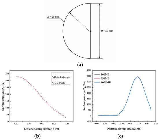
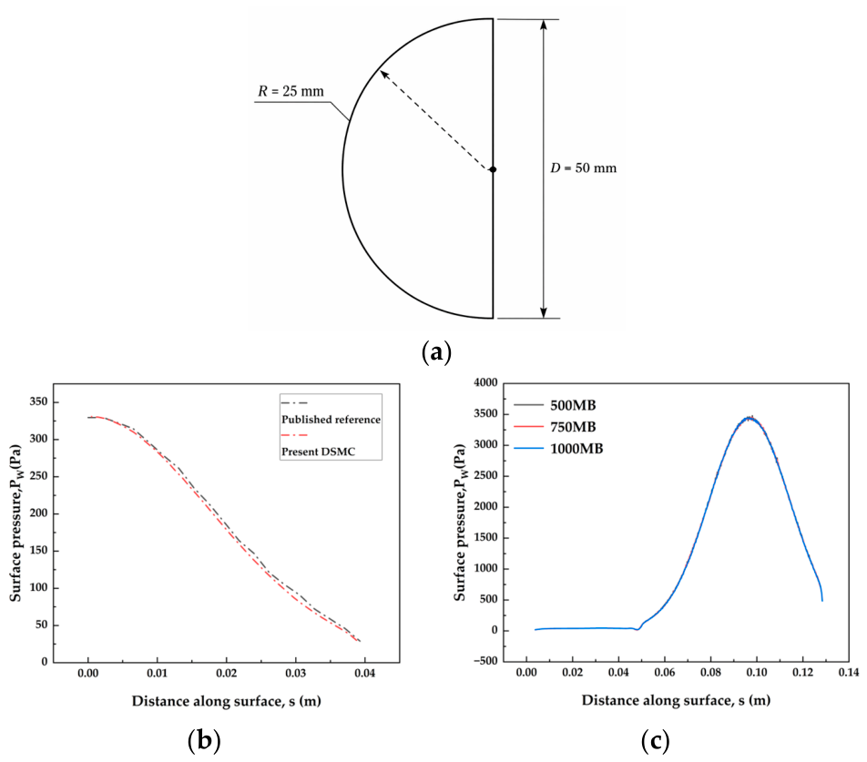
The symbolic regression method is first validated on a two-dimensional blunt-body aerodynamic dataset. The dataset is generated by the DSMC method. The two-dimensional semicircular blunt body is adopted as a simplified canonical configuration for the initial validation of the proposed modeling framework. Its simple geometry facilitates the investigation of the effects of Mach number, angle of attack, and rarefaction on the lift coefficient without introducing additional geometric complexity. The purpose of this configuration is not to represent a specific practical high-speed vehicle, but to provide a controlled test case for evaluating the proposed modeling method. The reference lift coefficients used in this study are obtained directly from DSMC simulations rather than from Euler- or RANS-based CFD calculations. The blunt body has a two-dimensional semicircular head with a radius of 25 mm. The geometric model is shown in Figure 1. The DSMC simulations were performed using the DS2V program. The computational domain was x ∈ [−0.08,0.05] m and y ∈ [−0.04,0.04] m. Stream boundary conditions were imposed on the outer boundaries, while the solid surface was modeled using diffuse reflection with a wall temperature of 300 K and a rotational energy accommodation coefficient of 1.0. The standard computational parameters of DS2V were employed, with adaptive collision and sampling cells used during the calculations. The reliability of the DSMC calculations was further examined through literature validation and a computational-resolution independence study. For validation, the surface-pressure distribution of a corresponding no-jet blunt-body case was compared with the data digitized from Ref. [31]. As shown in Figure 1b, the predicted surface-pressure distribution agrees well with the published reference data for the semicircular blunt-body configuration. In addition, three computational resolutions corresponding to 500, 750, and 1000 MB were examined for a representative condition. The resulting surface-pressure distributions are nearly identical, as shown in Figure 1c, indicating that the calculated wall pressure is insensitive to further increases in computational resolution. The freestream parameters are as follows. The Mach number ranges from 5 to 10. The angle of attack ranges from −10° to 20°. The Knudsen number ranges from 0.001 to 1. In this study, the freestream Knudsen number is defined as Kn = λ_∞/L_C, where λ_∞ is the freestream molecular mean free path and L_C is the characteristic length. The radius of the two-dimensional semicircular blunt body, Lc = R = 25 mm, is adopted as the characteristic length throughout the two-dimensional DSMC analysis. A total of 60 samples are designed using the optimal Latin hypercube sampling method. The Knudsen number spans multiple orders of magnitude. A logarithmic transformation is therefore applied. The transformed variable is $\ln kn$. This enhances the ability of symbolic regression to capture nonlinear relationships. The input feature vector is [Ma, α, lnkn]. The output target is the lift coefficient C_L. All 60 samples are used for five-fold cross-validation. In each fold, the training set and test set are split in a 4:1 ratio.

Figure 1. DSMC configuration and numerical verification: (a) geometric configuration of the two-dimensional blunt body; (b) comparison of the present DSMC surface-pressure distribution with the published reference data; (c) computational-resolution independence of the surface-pressure distribution using 500, 750, and 1000 MB settings.

The procedure in Section 2 is applied to the two-dimensional dataset. Five independent PySR searches are performed in each training fold, and the symmetry constraint C_L = 0 is imposed at alpha = 0. All representative equations satisfy the zero-lift physical constraint. They also achieve R² values above 0.997 on the test set, indicating that symbolic regression captures the dominant lift-coefficient behavior in a stable way.

Representative equations are obtained after PySR-score ranking and are listed in Table 1. The complete representative expressions for all five folds are provided in Appendix A.1 (Table A1).

Table 1. Representative equations and training/test performance for each fold.

Fold	Complexity	Train R2	Train MSE	Test R2	Test MSE
1	10	0.999747	6.0 × 10−6	0.999710	4.0 × 10−6
2	7	0.999238	1.7 × 10−5	0.997871	4.2 × 10−5
3	12	0.999768	4.8 × 10−6	0.999645	1.0 × 10−5
4	10	0.999710	6.5 × 10−6	0.999868	2.2 × 10−6
5	10	0.999772	4.6 × 10−6	0.999501	1.3 × 10−5

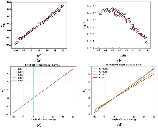
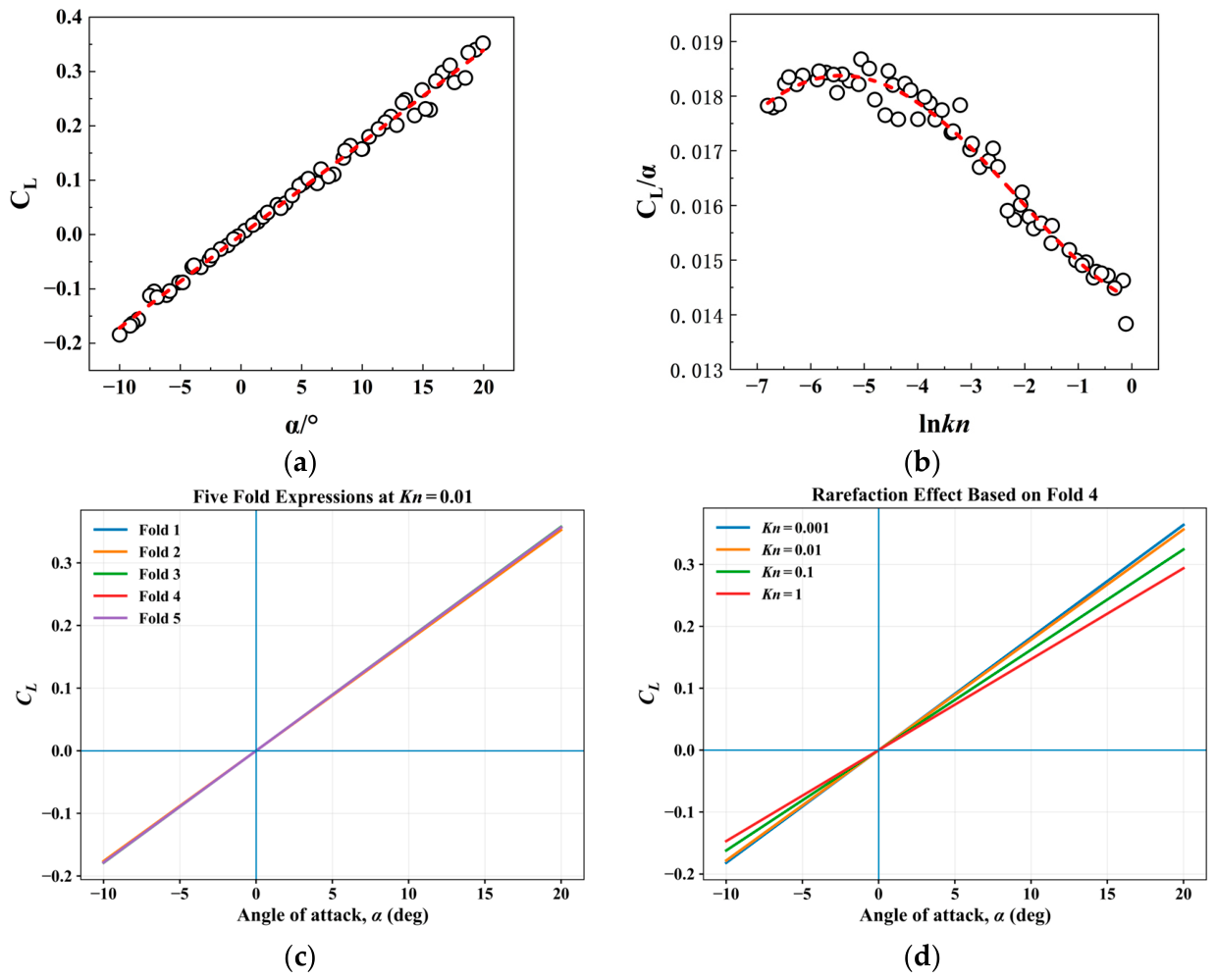
The training and test metrics are both reported in Table 1 to provide a more comprehensive assessment of the model performance for each fold. The close agreement between the training and test R² and MSE values indicates that the symbolic regression models maintain consistent performance on unseen samples, with no evident overfitting across the five folds. The coefficients differ across folds. The overall structures, however, are similar. Most equations are products of an angle-of-attack factor and a nonlinear function of lnkn. This indicates that symbolic regression identifies the dominant relationship of the lift coefficient consistently. To further evaluate the adequacy of the 60-sample dataset, a sample-size sensitivity analysis was conducted using 30, 40, 50, and 60 samples. The average test R² remained above 0.9994 for all sample sizes, with all five folds remaining valid and the test MSE on the order of (10⁻⁵). The consistently high cross-validation accuracy and stable fold-wise performance indicate good robustness and generalization capability, supporting the adequacy of 60 samples for the present problem. Figure 2 presents the relationships observed directly from the original 60 O-LHS DSMC samples rather than predictions from the explicit expression. Because Mach number, angle of attack, and Knudsen number vary simultaneously according to the O-LHS design, the remaining parameters are not held constant in either panel. Therefore, some scatter is expected when the multi-dimensional dataset is displayed in a two-dimensional form. As shown in Figure 2, C_L is approximately linear with α in the current parameter range. The ratio C_L/α varies nonlinearly with lnkn. The rational fraction structures in most folds describe the effects of rarefaction on the lift-curve slope better than the linear form in Fold 2. The fourth-fold expression is selected as the representative explicit model for the two-dimensional case. Prediction accuracy and expression simplicity are both considered. The selected equation is:

$$C_L=\alpha \left({\displaystyle \frac{0.06441}{{(\ln K_n)}^3-17.45}}+0.01838\right)$$

(7)

Figure 2. Relationships observed in the original 60 O-LHS DSMC samples: (a) C_L versus angle of attack α; (b) C_L/α versus lnKn. Each point represents an individual DSMC sample, and the other input parameters vary according to the O-LHS design. (c) CL–α relationships predicted by the five fold-representative expressions at Kn = 0.01; (d) influence of Knudsen number on the CL–α relationship predicted by the Fold-4 representative expression.

This expression has a complexity of 10. Its form is relatively simple. This expression achieves R² = 0.999868 and MSE = 2.2 × 10⁻⁶ on the test set. It approximates the two-dimensional DSMC data well. The expression can be interpreted in the form C_L = αf(lnKn). The explicit angle-of-attack factor shows that the lift coefficient is mainly governed by the angle of attack and satisfies the zero-lift symmetry condition at zero angle of attack. The function f(lnKn) represents an effective lift-curve slope modified by rarefaction effects. Within the investigated parameter range, the variation in f(lnKn) shows that stronger rarefaction changes the sensitivity of the lift coefficient to the angle of attack. The Mach number does not appear explicitly in the selected expression. This does not mean that Mach number has no physical influence. Within the present Ma = 5–10 range, the effects of angle of attack and rarefaction are more dominant, while the additional contribution of Mach number is relatively small. The weak Mach-number dependence may be related to the restricted hypersonic Mach-number range and the symmetric semicircular blunt-body geometry. The subsonic airfoil relation mentioned by the reviewer is therefore not directly applicable to the present rarefied hypersonic blunt-body flow. The current dataset cannot fully separate the effects of Mach-number range and geometry. Figure 2c compares the C_L −α relationships predicted by the five fold-representative expressions at Kn = 0.01. The nearly overlapping curves show consistent angle-of-attack dependence across folds. Figure 2d shows that the lift-curve slope decreases as Kn increases, indicating reduced lift sensitivity under stronger rarefaction. None of the five expressions contains an explicit Mach-number term; therefore, for these expressions, the predicted C_L remains unchanged with Mach number at fixed α and Kn within the present Ma = 5–10 range.

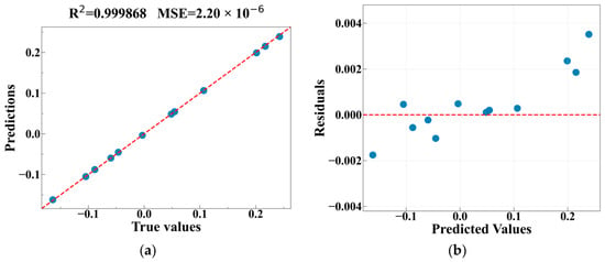
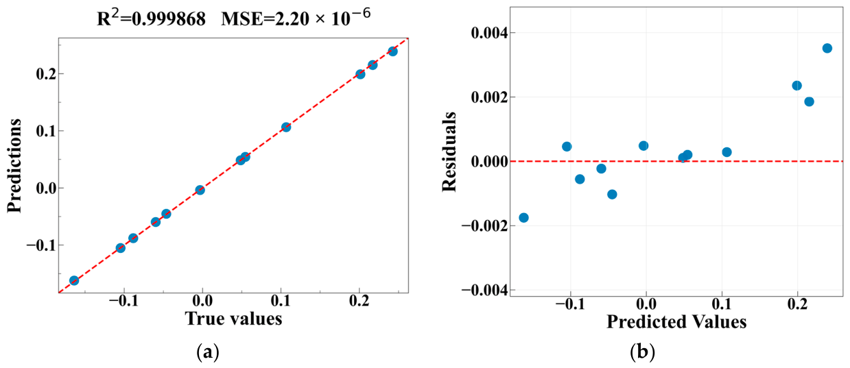
Figure 3 shows the prediction performance of the two-dimensional representative expression. The predicted values are close to the true values and lie near the ideal diagonal line in Figure 3a. Figure 3b further shows the residual distribution of the representative expression. Most residuals are distributed close to zero, indicating that the model does not exhibit an obvious systematic deviation over most of the prediction range. At low and moderate lift-coefficient levels, the residuals fluctuate around zero with relatively small magnitudes. However, several positive residuals appear at higher lift-coefficient levels, indicating a slight underestimation of the lift coefficient in this region. This deviation may be attributed to the approximately linear dependence on the angle of attack in the selected symbolic expression, which cannot fully capture the weak nonlinear aerodynamic effects occurring at relatively large angles of attack. Nevertheless, the residuals remain small overall, consistent with the high prediction accuracy of the model (R² = 0.999868, MSE = 2.2 × 10⁻⁶).

Figure 3. Fitting effect and residual distribution of the final explicit expression on the test set: (a) True values vs. predictions. (b) Residual distribution.

Linear regression, quadratic polynomial regression, and Kriging are used as benchmark models. The same training and test samples are used for all comparisons. Table 2 shows the prediction performance of these models.

Table 2. Performance of benchmark models.

Model	R2	MSE
Linear regression	0.9893	1.785 × 10−4
Quadratic polynomial regression	0.9977	3.837 × 10−5
Kriging	0.9997	5.155 × 10−6

The linear regression expression is:

$$C_L=-0.016068+4.62\times {10}^{-4}Ma+0.017132\alpha -2.970\times {10}^{-3}\ln (Kn)$$

(8)

The quadratic polynomial regression expression is:

$$\begin{array}{cc}{C}_L& =-0.040871+7.525\times {10}^{-3}Ma+0.015386\alpha -8.696\times {10}^{-3}\ln (Kn)-3.73\times {10}^{-4}M{a}^2-\hfill \\ & 4.7\times {10}^{-5}Ma\alpha +3.91\times {10}^{-4}Ma\ln (Kn)-2.7\times {10}^{-5}{\alpha }^2-5.97\times {10}^{-4}\alpha \ln (Kn)-\hfill \\ & 7.96\times {10}^{-4}{\ln }^2(Kn)\hfill \end{array}$$

(9)

Linear regression has the simplest form. It cannot capture the nonlinear variation in C_L/α with lnKn. Quadratic polynomial regression improves prediction accuracy, but its functional form remains constrained by the predefined polynomial order. Kriging further improves the prediction accuracy, achieving R² = 0.9997 and MSE = 5.155 × 10⁻⁶. Symbolic regression achieves a slightly higher accuracy (R² = 0.999868, MSE = 2.2 × 10⁻⁶) while providing a compact explicit expression without requiring a predefined functional form.

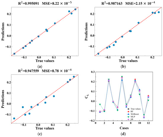
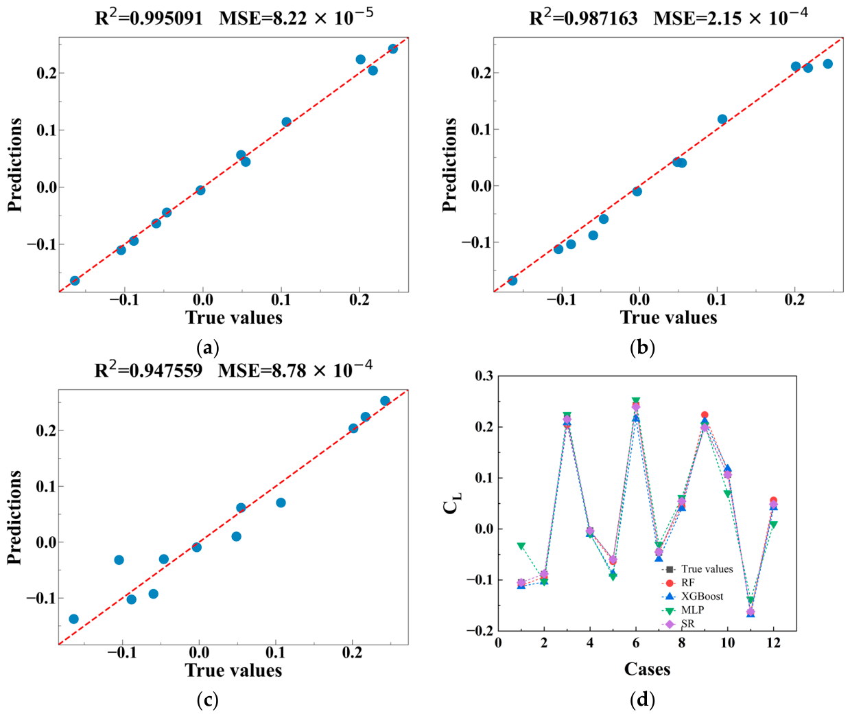
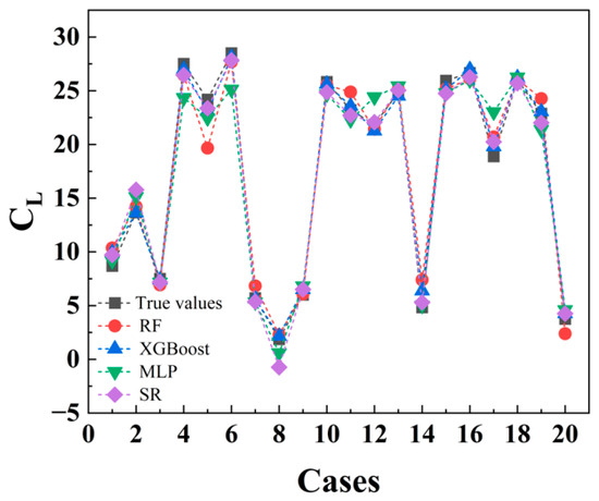
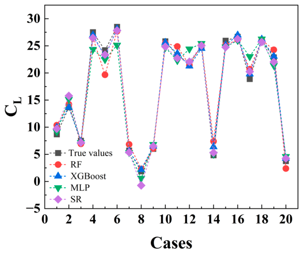
Random forest (RF), XGBoost, and multilayer perceptron (MLP) are also used as baseline models with the same training and test splits. Figure 4 shows the prediction results, and Table 3 lists the quantitative metrics. In Figure 4d, the horizontal axis represents the sequential indices of the 12 samples in the fixed test set rather than a physical input parameter. Each test sample corresponds to a different combination of Mach number, angle of attack, and Knudsen number. In the two-dimensional case, symbolic regression outperforms XGBoost and MLP and reaches accuracy comparable to random forest. Unlike black-box models, symbolic regression provides an explicit algebraic expression for interpretation, parameter analysis, and engineering use. For a fair comparison, the hyperparameters of RF, XGBoost, and MLP are tuned through grid search with three-fold cross-validation on the training set. The MLP input features are standardized. The 95% confidence intervals of R² are estimated by Bootstrap resampling with 100 iterations, and stability is evaluated using the mean and standard deviation of R² from five-fold cross-validation.

Figure 4. Comparison of prediction results between symbolic regression and black-box models: (a) RF. (b) XGBoost. (c) MLP. (d) Symbolic regression vs. black-box models.

Table 3. Quantitative comparison of lift coefficient among multiple models.

Metric	Symbolic Regression	RF	XGBoost	MLP
R2	0.999868	0.995091	0.987163	0.947559
MSE	2.2 × 10−6	8.22 × 10−5	2.15 × 10−4	8.78 × 10−4

3.2. Three-Dimensional Validation

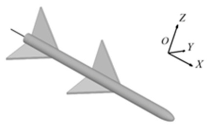
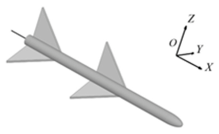
The symbolic regression method is further extended to a three-dimensional missile configuration. This evaluates its applicability to complex geometries and continuum flow conditions. The missile aerodynamic dataset published by Xiao et al. [11] is used. The dataset contains 196 missile shapes. Each shape has 915 flow conditions. The Mach number takes three values: 1.5, 2.0, and 2.5. The angle of attack takes 61 values from 0° to 60° in 1° increments. The sideslip angle takes five values: 0°, 10°, 20°, 30°, and 40°. The 70th shape is selected for this study. Its geometry is shown in Figure 5. To evaluate the capability of symbolic regression under limited-sample conditions, 100 samples were initially selected from the 915 available flow conditions as the baseline dataset. The influence of dataset size is further investigated using progressively enlarged datasets in Section 3.3.

Figure 5. Missile configuration.

Five-fold cross-validation is performed on the three-dimensional dataset. All folds achieve R² > 0.98. Symbolic regression builds an explicit mapping between input parameters and lift coefficient. This is accomplished with limited samples in three-dimensional space.

Representative expressions and training/test performance for each fold are shown in Table 4. The complete representative expressions for all five folds are provided in Appendix A.2 (Table A2).

Table 4. Representative equations and training/test performance for each fold.

Fold	Complexity	Train R2	Train MSE	Test R2	Test MSE
1	18	0.986751	1.048382	0.981205	1.286759
2	17	0.989680	0.771462	0.988117	1.043895
3	17	0.985916	1.058045	0.987760	1.032818
4	18	0.987713	1.004049	0.983746	0.951519
5	18	0.984732	1.157977	0.989615	0.842877

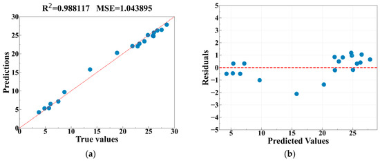
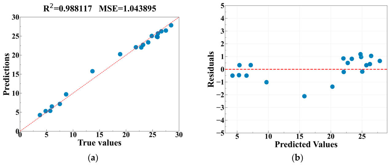
As shown in Table 4, the training and test performances are generally consistent across the five folds. The R² values remain above 0.98 for both the training and test sets, and no substantial performance degradation is observed on the test sets, indicating good generalization performance and no evident overfitting within the present dataset. The second-fold expression is selected as the representative explicit model for the three-dimensional case. The selection considers prediction accuracy, expression complexity, and clarity of variable relationships. Folds 1, 4, and 5 contain noticeable constant or bias terms, which reduce interpretability. Fold 3 has a structure similar to Fold 2 but slightly lower test accuracy. Fold 2 reaches R² = 0.988117 and MSE = 1.043895 on the test set. Its structure remains compact, captures the dominant role of angle of attack, and includes corrections for Mach number and sideslip angle. The selected expression is:

$$C_L=0.42687875\alpha +{\displaystyle \frac{0.85372907\alpha }{Ma}}-{\displaystyle \frac{0.00026525353{\alpha }^3}{Ma}}-5.147\times {10}^{-5}{\beta }^3$$

(10)

The model is built on 100 random samples. Its coefficients are valid within the current parameter range. Its extrapolation capability requires further validation with larger datasets. In the three-dimensional expression, the angle of attack gives the dominant contribution to the lift coefficient, consistent with its primary role in lift generation. The leading linear term in α describes the primary lift response to the angle of attack. The α/Ma and α³/Ma terms show that Mach number modifies both the approximately linear and nonlinear angle-of-attack contributions. Within the investigated parameter range, these Mach-related corrections decrease in magnitude as the Mach number increases. The cubic sideslip-angle term β³ represents a nonlinear correction associated with sideslip effects. The expression therefore reflects the combined effects of angle of attack, Mach number, and sideslip angle on the lift coefficient. The resulting expression is a data-driven analytical relation within the investigated parameter range, rather than a universal aerodynamic law.

Figure 6 shows the prediction performance of the second-fold expression. The predicted values are close to the true values in Figure 6a. The residuals fluctuate around zero in Figure 6b, although local deviations remain because of the limited sample size and uneven parameter-space coverage. These results show that symbolic regression can obtain a reasonably accurate explicit formula for a small-sample three-dimensional case, but local prediction accuracy still depends on sample distribution.

Figure 6. Fitting effect and residual distribution of the 2nd-fold final explicit expression on the test set: (a) True values vs. predictions. (b) Residual distribution.

To further assess the generalization capability of the selected explicit expression, an independent hold-out validation was performed using 20 previously unused flow conditions from the same published aerodynamic database. These validation cases were not used in model construction or cross-validation, and they cover all Mach-number and sideslip-angle levels considered in the original dataset, together with a broad range of angles of attack. For these hold-out cases, the explicit model achieves R² = 0.988681, MSE = 0.872781, RMSE = 0.934228, and MAE = 0.738954, which is consistent with the internal cross-validation performance (R² = 0.988117, MSE = 1.043895). This result indicates good predictive capability for unseen flow conditions within the investigated parameter range.

Linear regression, quadratic polynomial regression and Kriging are used to further evaluate the advantages of symbolic regression on the three-dimensional complex configuration. The same training and test samples are used for all comparisons. Table 5 shows the prediction performance of these models.

Table 5. Performance of benchmark models.

Model	R2	MSE
Linear regression	0.8270	15.196
Quadratic polynomial regression	0.9754	2.159
Kriging	0.9962	0.3328

The linear regression expression is:

$$C_L=12.071180-2.858445Ma-0.086254\beta +0.432592\alpha$$

(11)

The quadratic polynomial regression expression is:

$$\begin{array}{c}{C}_L=5.867898-4.220643Ma+0.044441\beta +1.157837\alpha +0.313667M{a}^2+\\ \hspace{1em}\hspace{1em}\hspace{1em}0.033721Ma\beta -0.008181Ma\alpha -0.004805{\beta }^2-0.000066\beta \alpha -0.012106{\alpha }^2\end{array}$$

(12)

Linear regression fails to capture the nonlinear relationships. Quadratic polynomial regression improves accuracy, but its functional form remains constrained by the predefined polynomial order. Kriging achieves the highest prediction accuracy among these benchmark models, with R² = 0.9962 and MSE = 0.3328. Symbolic regression achieves R² = 0.988117 and MSE = 1.043895. Although its prediction accuracy is lower than that of Kriging, symbolic regression directly provides a compact and interpretable explicit expression without requiring a predefined functional form.

RF, XGBoost, and MLP are also compared. Figure 7 shows the prediction results, and Table 6 lists the quantitative metrics. XGBoost achieves the highest prediction accuracy, while symbolic regression gives lower accuracy than XGBoost but performs better than RF and MLP. Black-box models therefore have a higher accuracy ceiling under small-sample three-dimensional conditions. The key advantage of symbolic regression is its explicit algebraic expression, which supports interpretation and engineering application. The hyperparameters of RF, XGBoost, and MLP are tuned through grid search with cross-validation on the training set. The 95% confidence intervals of R² are estimated by Bootstrap resampling.

Figure 7. Comparison of prediction results between symbolic regression and black-box models.

Table 6. Quantitative comparison of lift coefficient among multiple models.

Metric	Symbolic Regression	RF	XGBoost	MLP
R2	0.988117	0.974447	0.995118	0.965718
MSE	1.043895	2.244749	0.428827	3.011479

3.3. Effect of Sample Size on Symbolic Regression Performance

To further investigate the influence of dataset size on prediction accuracy, model complexity, and computational cost, nested datasets containing 100, 200, 400, and 600 samples were considered. The same five-fold cross-validation procedure and symbolic-regression settings were applied to all datasets. In addition to the prediction metrics, the average complexity of the representative expressions and the total computation time were recorded for comparison.

Table 7 shows the results. All sample sizes achieve high prediction accuracy, with average R² values remaining around 0.98. Symbolic regression therefore remains stable in three-dimensional explicit modeling. When the sample size increases from 100 to 200, prediction accuracy does not improve markedly, but the variable composition of the expressions becomes more consistent. This trend suggests that more samples help identify dominant variable relationships. At 400 samples, the best candidate expression reaches R² = 0.994136 and MSE = 0.534041. At 600 samples, the accuracy remains stable, and no further notable improvement appears. Sample size therefore does not guarantee monotonic improvement in prediction accuracy.

Table 7. The performance of symbolic regression models under different three-dimensional sample sizes.

Sample Size	Valid Folds	Average Complexity	Computation Time (min)	Average R2	Best R2	Average MSE	Best MSE
100	5/5	17.40	26.86	0.985889	0.989615	1.031574	0.842877
200	5/5	17.60	27.28	0.984146	0.986492	1.135817	0.845272
400	4/5	17.25	34.21	0.982953	0.994136	1.194401	0.534041
600	5/5	17.75	39.24	0.983593	0.987410	1.155646	0.893590

Expression structures vary considerably at 100 samples. This suggests that symbolic regression results are sensitive to data splits and search randomness under small-sample conditions. At 200 samples, terms related to α, α³, β³ and Ma appear frequently across folds. The identification of main variables becomes more stable. When the sample size is further increased to 400 and 600, the algebraic forms vary across folds. The overall relationship remains consistent: angle of attack dominates, and Mach number and sideslip angle serve as corrections. Symbolic regression therefore identifies the dominant variable relationships in the three-dimensional lift coefficient across different sample sizes. In addition, the average expression complexity remains within a narrow range of 17.25–17.75 as the sample size increases, indicating that larger datasets do not necessarily lead to more complex symbolic expressions. Meanwhile, the computation time increases from 26.86 min for 100 samples to 39.24 min for 600 samples. These results indicate that increasing the dataset size does not produce a monotonic improvement in prediction accuracy, while the model complexity remains relatively stable and the computational cost generally increases.

Table 7 shows no strict monotonic improvement in model accuracy with increasing sample size. Larger samples cover a broader range of flow conditions, and the model must fit local nonlinearities at different angles of attack, sideslip angles, and Mach numbers. Under the complexity constraint, symbolic regression balances global accuracy and expression simplicity. Performance variation across sample sizes is therefore expected.

Symbolic regression models maintain high prediction accuracy across all sample sizes. The expressions consistently include a dominant angle-of-attack term, high-order angle corrections, sideslip corrections, and Mach-related terms. These features confirm that the explicit three-dimensional lift-coefficient formulas are not artifacts of one small sample. Sample size mainly affects expression stability and local prediction errors, rather than producing a simple monotonic accuracy improvement.

4. Conclusions

(1)

This study develops a robust modeling framework that combines five-fold cross-validation, multiple independent runs, and symmetry-constrained screening. The framework selects explicit expressions that satisfy basic physical laws from sample data.

(2)

In the two-dimensional blunt-body case, symbolic regression obtains an analytical model that satisfies the zero-lift constraint at zero angle of attack. The model captures the nonlinear influence of the Knudsen number on the lift-curve slope and achieves high prediction accuracy.

(3)

In the three-dimensional missile case, symbolic regression builds a reasonably accurate explicit expression with only 100 samples. The nested-sample results from 100 to 600 samples show that the model maintains high accuracy across different sample sizes. The expressions consistently identify the dominant role of angle of attack and the corrective effects of Mach number and sideslip angle.

(4)

Compared with linear regression and quadratic polynomial regression, symbolic regression achieves higher accuracy while satisfying physical constraints. It does not require a predefined functional form. Kriging provides comparable or higher predictive accuracy, while symbolic regression provides a more compact and directly interpretable algebraic expression. Compared with black-box models such as RF, XGBoost, and MLP, symbolic regression provides explicit algebraic expressions that support interpretation, editing, and engineering integration.

Larger sample sizes do not guarantee monotonic accuracy improvement. Sample distribution and search randomness still affect the results. Further validation using independent aerodynamic datasets or different configurations is still needed to assess generalization beyond the investigated parameter range.

Appendix A.1

Table A1. Representative equations for each fold (two-dimensional blunt body).

Fold	Representative Equation
1	$C_L=\alpha \left({\displaystyle \frac{0.06627}{{(\ln \mathrm{Kn})}^3-18.04}}+0.01839\right)$
2	$C_L=\alpha \left(-0.0006453\ln K_n+0.01465\right)$
3	$C_L=\alpha \left({\displaystyle \frac{0.003645}{{(0.3739\ln K_n)}^3-0.9548}}+0.01848\right)$
4	$C_L=\alpha \left({\displaystyle \frac{0.06441}{{(\ln K_n)}^3-17.45}}+0.01838\right)$
5	$C_L=\alpha \left({\displaystyle \frac{0.04820}{{(\ln K_n)}^3-13.37}}+0.01827\right)$

Table A1. Representative equations for each fold (two-dimensional blunt body).

Fold	Representative Equation
1	$C_L=\alpha \left({\displaystyle \frac{0.06627}{{(\ln \mathrm{Kn})}^3-18.04}}+0.01839\right)$
2	$C_L=\alpha \left(-0.0006453\ln K_n+0.01465\right)$
3	$C_L=\alpha \left({\displaystyle \frac{0.003645}{{(0.3739\ln K_n)}^3-0.9548}}+0.01848\right)$
4	$C_L=\alpha \left({\displaystyle \frac{0.06441}{{(\ln K_n)}^3-17.45}}+0.01838\right)$
5	$C_L=\alpha \left({\displaystyle \frac{0.04820}{{(\ln K_n)}^3-13.37}}+0.01827\right)$

Appendix A.2

Table A2. Representative equations for each fold (three-dimensional missile).

Fold	Representative Equation
1	$C_L=3.8123-0.8738267M{a}^2+0.8738267\alpha -1.393\times {10}^{-4}{\alpha }^3-5.600\times {10}^{-5}{\beta }^3$
2	$C_L=0.42687875\alpha +{\displaystyle \frac{0.85372907\alpha }{Ma}}-{\displaystyle \frac{0.00026525353{\alpha }^3}{Ma}}-5.147\times {10}^{-5}{\beta }^3$
3	$\begin{array}{c}{C}_L=0.6245848\alpha +{\displaystyle \frac{0.5021206\alpha }{Ma}}-1.006\times {10}^{-4}{\alpha }^3-\\ 3.713\times {10}^{-5}{\beta }^3-{\displaystyle \frac{8.087\times {10}^{-5}{\alpha }^3}{Ma}}-{\displaystyle \frac{2.985\times {10}^{-5}{\beta }^3}{Ma}}\end{array}$
4	$\begin{array}{c}{C}_L=4.03023-0.85889715M{a}^2+0.85889715\alpha -\\ 1.4771047\times {10}^{-4}{\alpha }^3+1.4771047\times {10}^{-4}M{a}^2{\alpha }^2-5.8212237\times {10}^{-5}{\beta }^3\end{array}$
5	$C_L=3.9346843-0.86990845M{a}^2+0.86990845\alpha -1.393\times {10}^{-4}{\alpha }^3-5.599\times {10}^{-5}{\beta }^3$

Table A2. Representative equations for each fold (three-dimensional missile).

Fold	Representative Equation
1	$C_L=3.8123-0.8738267M{a}^2+0.8738267\alpha -1.393\times {10}^{-4}{\alpha }^3-5.600\times {10}^{-5}{\beta }^3$
2	$C_L=0.42687875\alpha +{\displaystyle \frac{0.85372907\alpha }{Ma}}-{\displaystyle \frac{0.00026525353{\alpha }^3}{Ma}}-5.147\times {10}^{-5}{\beta }^3$
3	$\begin{array}{c}{C}_L=0.6245848\alpha +{\displaystyle \frac{0.5021206\alpha }{Ma}}-1.006\times {10}^{-4}{\alpha }^3-\\ 3.713\times {10}^{-5}{\beta }^3-{\displaystyle \frac{8.087\times {10}^{-5}{\alpha }^3}{Ma}}-{\displaystyle \frac{2.985\times {10}^{-5}{\beta }^3}{Ma}}\end{array}$
4	$\begin{array}{c}{C}_L=4.03023-0.85889715M{a}^2+0.85889715\alpha -\\ 1.4771047\times {10}^{-4}{\alpha }^3+1.4771047\times {10}^{-4}M{a}^2{\alpha }^2-5.8212237\times {10}^{-5}{\beta }^3\end{array}$
5	$C_L=3.9346843-0.86990845M{a}^2+0.86990845\alpha -1.393\times {10}^{-4}{\alpha }^3-5.599\times {10}^{-5}{\beta }^3$

References

- Zhang, L. Application Research of DSMC and Bridge Function Method in Aerodynamic Force Calculation of Long-Range Projectile in Transition Flow Region. Master’s Thesis, Nanjing University of Science and Technology, Nanjing, China, 2019. [Google Scholar]
- Barlow, J.B.; Rae, W.H.; Pope, A. Low-Speed Wind Tunnel Testing, 3rd ed.; Wiley: New York, NY, USA, 1999. [Google Scholar]
- Wu, X.; Chen, W.F.; Shi, Y.Z. DSMC Simulation and Bridge Function Estimation of Aerodynamic Characteristics for Complex Configuration. Missiles Space Veh. 2003, 3, 51–56. [Google Scholar]
- Zhao, J.; Zeng, L.; Shao, X. A Novel Prediction Method for Unsteady Aerodynamic Force on Three-Dimensional Folding Wing Aircraft. Aerosp. Sci. Technol. 2023, 137, 108287. [Google Scholar] [CrossRef] [Scilit]
- Li, N.; Liu, Y.; Gong, G.; Zhao, L.; Yuan, H. A Generative Deep Learning Approach for Real-Time Prediction of Hypersonic Vehicles in Fluid-Thermo-Structural Coupling Fields. Aerosp. Sci. Technol. 2023, 139, 108398. [Google Scholar] [CrossRef] [Scilit]
- Liu, Z.; Guo, C.P.; Li, H.Y.; Cui, R.F. Fast Prediction Method of Aircraft Aerodynamic Force Based on Ensemble Learning. Aeronaut. Sci. Technol. 2024, 35, 13–18. [Google Scholar]
- Mostafa, A.; Adel, M.; Suliman, M.M.; Milad, M.; Zamel, A.A. Data-Efficient AI Models for Aerodynamic Coefficient Prediction: A Case Study on NACA Airfoils with Minimal CFD Runs. Beni-Suef Univ. J. Basic Appl. Sci. 2026, 15, 31. [Google Scholar] [CrossRef] [Scilit]
- Zhao, K.N. Aerodynamic Force Prediction of Aero-Engine Compressor Blade Based on Machine Learning. Master’s Thesis, Tiangong University, Tianjin, China, 2025. [Google Scholar]
- Wu, S.H. Prediction of Aerodynamic Force at Compressor Blade Tip of Aero-Engine Based on Machine Learning. Master’s Thesis, Tiangong University, Tianjin, China, 2025. [Google Scholar]
- Li, Y.R. Aerodynamic Characteristic Prediction of Two-Dimensional Rectangular Cylinder Based on Machine Learning. Master’s Thesis, Harbin Institute of Technology, Harbin, China, 2024. [Google Scholar]
- Xiao, Q.S.; Chen, X.H.; Chen, W.F.; Liu, Y.; Gao, S.J.X.; Li, K.; Pang, Y.; Liu, J. Intelligent Prediction Method of Aerodynamic Coefficient for Aircraft. J. Natl. Univ. Def. Technol. 2026, 48, 88–98. [Google Scholar]
- Liu, X.B.; Zeng, L.; Long, Y.; Shao, Y.P. Aerodynamic Coefficient Prediction Method for Aircraft Based on Automatic Feature Construction. Comput. Digit. Eng. 2025, 53, 2278–2283. [Google Scholar]
- Liu, L.; Yang, C.M.; Lin, J.Z.; Xiang, H.H. Missile Aerodynamic Coefficient Prediction Based on Deep Metric Learning. J. Nanjing Univ. Aeronaut. Astronaut. 2024, 56, 950–959. [Google Scholar]
- Shajaripour, M.; Zeraatgar, H. Investigating the Aerodynamic Characteristics of High-Speed Planing Catamarans through Wind Tunnel Tests, CFD Simulations, and Regression Analysis. Ocean Eng. 2025, 338, 121950. [Google Scholar] [CrossRef] [Scilit]
- Zhang, Z.C.; Gao, T.Y.; Zhang, L.; Tuo, S.F. Aeroheating Agent Model Based on Radial Basis Function Neural Network. Acta Aeronaut. Astronaut. Sin. 2021, 42, 303–312. [Google Scholar]
- Akbal, Ö.; Kaya, M.O.; Şahin, A.D. An Integrated CFD-Based Reduced-Order Model for Rapid Prediction of In-Flight Ice Accretion and Aerodynamic Degradation on the NACA 0012 Airfoil. Aerosp. Sci. Technol. 2026, 168, 111153. [Google Scholar] [CrossRef] [Scilit]
- Gao, X.; Lian, F.; Kong, Y.N.; Chen, G.; Zhang, G.; Wang, W. Nonlinear Fast Aerodynamic Modeling Based on Multivariate Orthogonal Functions. Acta Aerodyn. Sin. 2023, 41, 81–88. [Google Scholar]
- He, Z.Z.; Wu, C.Y.; Zhang, Y.F. A Field Inversion and Symbolic Regression Enhanced Spalart-Allmaras Model for Airfoil Stall Prediction. Phys. Fluids 2024, 36, 065111. [Google Scholar] [CrossRef] [Scilit]
- Zhang, H.; Shen, Y.; Huang, W.; Zhao, Z.; An, K.; Liu, S. Research Progress of Intelligent Flow Field Modeling Methods for Aircraft. J. Natl. Univ. Def. Technol. 2026, 48, 1–15. [Google Scholar]
- Luo, Y.Z. Research on Symbolic Regression Interpretation Method for Neural Networks. Master’s Thesis, China University of Petroleum (Beijing), Beijing, China, 2024. [Google Scholar]
- Hu, X.L. Research on Symbolic Regression Algorithm for Neural Network Interpretation. Master’s Thesis, China University of Petroleum (Beijing), Beijing, China, 2023. [Google Scholar]
- Tao, F. Research on Symbolic Regression Algorithm Based on Reinforcement Learning. Master’s Thesis, China University of Petroleum (Beijing), Beijing, China, 2019. [Google Scholar]
- Zhou, S. Research and Design of Symbolic Regression Algorithm Based on Space Partition. Master’s Thesis, China University of Petroleum (Beijing), Beijing, China, 2020. [Google Scholar]
- Jin, J.B.; Wu, P. Application of Genetic Programming in Symbolic Regression. Comput. Digit. Eng. 2009, 37, 13–16. [Google Scholar]
- Xu, P.C.; He, L.; Li, C.; Qian, W.Q.; Zhao, T. Deep Symbolic Regression Method Based on Transformer. J. Comput. Appl. 2025, 45, 1455–1463. [Google Scholar]
- Sheng, W.T. Research on Generalization Performance of Symbolic Regression Based on Multi-Objective Optimization. Master’s Thesis, Xi’an University of Technology, Xi’an, China, 2021. [Google Scholar]
- Wang, J.Y. Research on Symbolic Regression Algorithm for Fluid Mechanics. Master’s Thesis, China University of Petroleum (Beijing), Beijing, China, 2024. [Google Scholar]
- He, B.H. Research on Symbolic Regression under Data Feature Mechanism. Master’s Thesis, China University of Petroleum (Beijing), Beijing, China, 2023. [Google Scholar]
- Wang, D.; Chen, Y.; Chen, S. Discovering an Interpretable Mathematical Expression for a Full Wind-Turbine Wake with Artificial Intelligence Enhanced Symbolic Regression. Phys. Fluids 2024, 36, 105110. [Google Scholar] [CrossRef] [Scilit]
- Bendavid, J.; Conde, D.; Morales-Alvarado, M.; Sanz, V.; Ubiali, M. Angular Coefficients from Interpretable Machine Learning with Symbolic Regression. J. High Energy Phys. 2026, 2026, 189. [Google Scholar] [CrossRef] [Scilit]
- Ni, Z.J.; Fang, S.Z. Flow Field Characteristics of Opposing Jet at Blunted Leading Edge of Hypersonic Rarefied Flow. J. Propuls. Technol. 2024, 45, 2209046. [Google Scholar]
Disclaimer/Publisher’s Note: The statements, opinions and data contained in all publications are solely those of the individual author(s) and contributor(s) and not of MDPI and/or the editor(s). MDPI and/or the editor(s) disclaim responsibility for any injury to people or property resulting from any ideas, methods, instructions or products referred to in the content. |
© 2026 by the authors. Licensee MDPI, Basel, Switzerland. This article is an open access article distributed under the terms and conditions of the Creative Commons Attribution (CC BY) license.