


Abstract
In this paper, the stochastic responses of multi-degree-of-freedom (MDOF) linear/nonlinear systems with rational-order fractional derivatives excited by colored noise are investigated. A closed-form expression for the PSDs of MDOF linear systems with fractional derivatives under exponential colored noise is derived by combining the eigenvector expansion method (EEM) and the pole-residue representation of the transfer function. The equivalent linearization method (ELM) is developed to determine the stochastic responses of fractional-order nonlinear systems. This is achieved by replacing the original system with an equivalent fractional-order linear system whose parameters are determined by minimizing the mean-square difference. The EEM is incorporated into the linearization framework to solve the linear fractional-order equations during the iterative process for the equivalent coefficients. Two widely adopted linearization criteria, the energy-based criterion and the equation-based criterion, are examined in detail. Numerical examples, including two linear systems and three nonlinear fractional-order systems with various types of nonlinearity under colored noise, are presented to verify the accuracy and applicability of the proposed method. Compared with Monte Carlo (MC) simulations, both criteria provide satisfactory accuracy. In addition, the results from the energy-based linearization criterion are more accurate than those from the equation-based criterion for single-degree-of-freedom (SDOF) systems, whereas for MDOF systems, the equation-based criterion yields slightly more accurate results than the energy-based criterion. The effects of nonlinear intensity and the order of the fractional derivative on the response statistics are also investigated.
1. Introduction
Spacecraft (such as satellites, launch vehicles, etc.) are subjected to various mechanical loads during transportation and launch operations. Excessive vibrations can cause mechanical damage and failure, as well as instrument malfunctions, thereby compromising the safety and reliability of these systems. Viscoelastic damping materials (such as rubber and polymeric materials), which combine both elastic energy storage and viscous energy dissipation characteristics, have attracted considerable attention in the field of structural vibration and noise control. Accurate modeling of viscoelastic materials is imperative for enhancing mechanical vibration control and advancing the design of high-performance damped structures. The constitutive relationship of viscoelastic materials is a convolution integral, in which the stress depends not only on the current strain but also on the entire strain history. Fractional calculus has been demonstrated to be a powerful tool for accurately capturing the stress–strain relationship of viscoelastic materials using a few parameters due to its unique long-memory and non-local properties [1]. Compared to traditional integer-order constitutive models, fractional operators can provide higher accuracy in describing stress relaxation, creep, and the frequency-dependent loss factor due to their inherent ability to reflect the memory effects caused by the evolution of materials’ microstructure and energy dissipation processes. In particular, with regard to the control of broadband vibration problems, they can capture the power-law characteristics of the storage/loss modulus as a function of frequency in a compact mathematical form. Fractional operators have been widely applied in engineering, such as in isolation systems [2,3], viscoelastic dampers [4,5], and viscoelastic tuned mass dampers [6,7].
Random excitation is one of the predominant mechanical environments to which spacecraft are exposed, such as aerodynamic noise and vibrations generated by the operation of rocket engines. Mechanical structures containing viscoelastic materials under stochastic excitation can be described by stochastic fractional differential equations. In the context of random vibration analysis, the Monte Carlo approach, which is applicable to arbitrary systems subjected to any excitation, is the most general method and is frequently utilized to validate the accuracy of other approximate methods. This method involves the numerical solution of a large number of sample responses, followed by statistical analysis, resulting in relatively low computational efficiency. For linear systems with fractional derivatives, several methods have been proposed and can be broadly categorized into two main types: analytical/semi-analytical solutions and numerical methods. The first commonly used method is the frequency-domain method. Spanos and Zeldin [8] first proposed the frequency-domain solution for a linear oscillator with fractional derivatives. Barone et al. [6] studied the effects of fractional tuned mass dampers under Gaussian white noise using the frequency-domain method. Denoël [9] investigated the response of an SDOF linear oscillator with fractional derivatives subjected to colored noise using multiple-timescale spectral analysis. This method can efficiently determine the steady-state response; however, its disadvantage is that it is difficult to obtain transient or maximum peak responses. According to random vibration theory, the twofold integral method is an important tool for determining the stochastic response in the time domain. The crucial step in this method is determining the unit impulse response function (IRF), which can be derived using the Fourier transform [10], Laplace transform [11], Prony-SS method [12], or eigenvector expansion method [13]. However, it should be noted that the computational burden increases significantly in the presence of either prolonged operating periods or high dimensionality. Eigenvector expansion is considered a promising approach for determining the response of fractional-order systems since it can yield closed-form solutions to the IRF. Its application has been extended from deterministic excitation to stationary/nonstationary random excitation. Pinnola [14] presented an analytical expression of the response variance of a linear oscillator with fractional derivatives using complex moments and eigenvector expansion. Pirrotta et al. [15] provided time- and frequency-domain solutions to linear MDOF fractional-order systems. Kong et al. [13] obtained analytical solutions for the nonstationary responses of MDOF systems with 1/2-order fractional derivatives. Di Matteo and Spanos [16] obtained a closed-form solution for the evolutionary power spectral density (PSD) and the nonstationary response statistics using the eigenvector expansion method and the pole-residue representation. Xu et al. [17] presented an analytical solution for the nonstationary responses of linear systems with fractional derivatives. Note that the eigenvector expansion method is applicable only to fractional-order systems of rational order. Numerical methods are based on the numerical solution to fractional differential equations under deterministic excitation. An alternative strategy is the memory-free method (MFM), which converts fractional derivative terms into a set of first-order differential equations through variable transformation and discretization [18]. This method eliminates the need to store historical responses, thereby improving computational efficiency. Su and Xian [19] developed an explicit time-domain approach based on Newmark- for the stochastic analysis of linear fractional-order systems.
When performing stochastic analysis of nonlinear systems containing fractional derivatives, extending analytical/semi-analytical techniques for integer-order systems to fractional-order systems is a widely adopted strategy. The most prevalent approaches include the stochastic averaging method (SAM), equivalent linearization method (ELM), and path integral method. The stochastic averaging method [20,21,22] is applicable to the analysis of fractional nonlinear systems with light damping under broadband excitation. The equivalent linearization method has been identified as one of the most popular and useful approximate techniques for the stochastic analysis of nonlinear systems with fractional derivatives. Spanos and Evangelatos [23] employed the statistical linearization technique to determine the response of a fractional-order Duffing oscillator under white noise. Spanos and Zhang [24] determined the nonstationary responses of fractional nonlinear systems using the statistical linearization method. Xu et al. [25] studied fractional nonlinear systems under indivisible PSD excitation via statistical linearization and eigenvector expansion. Zhang et al. [26] and Zhao et al. [27] determined the nonstationary responses of hysteretic oscillators with fractional derivatives. Xian and Su [28] developed an explicit time-domain numerical method for addressing the nonstationary responses of nonlinear oscillators with fractional-order derivatives combined with the ELM. Combining the ELM with the SAM to determine the response statistics of fractional-order systems has also garnered considerable attention. Di Matteo et al. [29] determined the survival probabilities of fractional-order systems. The response probability density functions (PDFs) and survival probabilities of nonlinear systems with fractional derivatives under a given seismic design spectrum [30] and evolutionary excitation [31,32] were also determined using the ELM/SAM. Spanos and Pomaro [33] estimated the stationary response PSD of a polynomial nonlinear oscillator with fractional-order damping subjected to Gaussian white noise. Zhang et al. [34] proposed an approximate analytical method to determine the stochastic responses of fractionally nonlinear oscillators subjected to combined periodic and evolutionary excitations using the MFM [18] and the ELM/SAM. For fractional-order systems under stochastic and deterministic excitations, the equivalent linearization method remains effective, with the aid of the harmonic balance method [35,36,37]. Other approaches, such as the path integral method [38], have also been applied to study the stochastic responses of nonlinear oscillators with fractional derivatives.
The equivalent linearization method exhibits considerable adaptability for determining the stochastic responses of nonlinear fractional-order systems. Owing to its reliance on the Gaussian approximation of responses, accuracy may be slightly reduced when applied to strongly nonlinear systems. Nevertheless, it remains widely adopted due to its conceptual simplicity, wide range of applications, and ease of implementation. The responses of MDOF fractional-order linear/nonlinear systems excited by colored noise have received limited attention in the literature. In this paper, the determination of the stochastic responses of MDOF linear/nonlinear systems with fractional derivatives is addressed.
For MDOF linear systems with fractional derivatives under exponential colored noise, a closed-form analytical expression for the PSD is derived by combining the eigenvector expansion method with the pole-residue representation of the transfer function. The equivalent linearization method is developed to determine the response statistics of nonlinear fractional-order systems, and the EEM is used to calculate the statistical moments of linear fractional-order systems during the iterative process. Two widely adopted linearization criteria, the energy-based criterion and the equation-based criterion, are examined. The rest of this paper is organized as follows. Section 2 introduces the equivalent linearization method and the eigenvector expansion method for stochastic analysis. Further, numerical examples, including two linear systems with fractional derivatives and three nonlinear fractional-order systems with various types of nonlinearity excited by colored noise, are presented in Section 3. Finally, the conclusions are presented in Section 4.
2. Mathematical Formulation
2.1. Nonlinear Fractional-Order Systems Excited by Colored Noise
The equation of motion of an n-DOF nonlinear system with fractional derivatives subjected to stochastic excitations can be formulated as
where represent matrices for the mass, fractional-order damping, and stiffness of the system, respectively; are vectors for displacement, velocity, and acceleration; represents an vector of a nonlinear term; and is an -order fractional derivative of a displacement vector, where . The initial conditions are . In this paper, the Caputo definition for fractional derivatives is adopted, which is defined as
and denotes an excitation vector with the power spectral density (PSD)
where is the auto/cross-PSD of .
2.2. Equivalent Linearization of Nonlinear Systems with Fractional Derivatives
The system in Equation (1) is difficult to solve using analytical methods when the function G is non-zero and nonlinear, necessitating the use of approximate analytical or numerical techniques. The ELM provides a systematic and feasible framework for deriving an approximate solution of Equation (1) and is one of the most popular methods for random vibration analysis of nonlinear systems. The core concept of this method is to replace the fractional-order nonlinear dynamical system described by Equation (1) with an equivalent system that is easier to solve. This replacement is performed to optimize a specific metric that quantifies the difference between the two systems. For practical convenience, the equivalent system is restricted to be linear since only linear systems allow for more convenient treatment for MDOF systems with fractional derivatives.
The n-DOF equivalent linear system with fractional derivative elements can be expressed as
where are equivalent matrices for damping and stiffness. They are determined such that the difference between the two systems is minimized in the statistical sense.
It is imperative to establish a criterion for minimizing , defined in terms of an appropriate norm of the difference. In fact, only the mean-square criterion has been widely applied. The minimization of is performed according to the criterion
where denotes the mathematical expectation operation.
The necessary conditions for Equation (5) to be satisfied are
and
where and are the elements of the matrices and .
2.2.1. Equality of Mean-Square Deviation of Equations
The difference between the equations of the two systems can be written as
If both and are determined for the that is the solution to Equation (4), it is reasonable to hypothesize that this solution will also be a fairly good approximation to the solution of the nonlinear problem governed by Equation (1). It can be demonstrated that the solution to the equivalent linear system with fractional derivatives depends on and . Consequently, a cyclic relation may be established between , and . The system response can be determined once the equivalent coefficients and are obtained. At this stage it is evident that the weaker the system’s nonlinearity, the more suitable an equivalent linear system is for describing the response of the original system.
Upon using the linearity of the expectation operator , Equation (9) can be rewritten as
It can be seen that depends only on and . Thus, the minimization criterion can be expressed as
The parameters in and can be determined using the following expressions:
2.2.2. Equality of the Mean-Square Deviation of Potential and Dissipative Energy
Mechanical vibration is a dynamic process involving work and energy conversion, manifesting as the interaction between generalized forces and displacements. Consequently, a linearization technique based on the equivalent principle of work and energy can facilitate the generation of better statistical responses than the classical approach.
The potential energy of the nonlinear system is
where is the linear potential energy and represents the nonlinear potential energy. They can be written as
and
where is the nonlinear potential energy stored in the i-th element.
The potential energy of the equivalent system is
The difference in potential energy between the two systems is
According to the criterion of the minimum mean-square deviation of potential energy between the two systems, the equivalent stiffness coefficient is
To determine the equivalent damping coefficient, the energy dissipation function is defined as
The dissipative energy of the nonlinear system and the equivalent system can be calculated as follows:
and
The difference in dissipative energy between the two systems is
According to the criterion of the minimum mean-square deviation of dissipative energy between the two systems, the equivalent damping coefficient is
It should be emphasized that the Gaussian response assumption adopted here is an approximation rather than a general property of nonlinear spacecraft structures. This treatment is essentially a second-order statistical closure, in which the response is characterized by its mean and covariance. Therefore, the present formulation is suitable for systems with weak to moderate nonlinearity, where the response distribution remains close to Gaussian. The accuracy of the approximation depends on the type and strength of the structural nonlinearity. In the case of systems with strong nonlinearity, the system response may deviate from a Gaussian distribution, resulting in reduced accuracy. Strain-dependent damping, joint nonlinearities, stick-slip behavior, and local impact phenomena can lead to non-Gaussian response statistics. The validity of this assumption should be checked for specific applications, and the employment of Monte Carlo simulation, higher-order moment methods, polynomial chaos expansion, or other improved techniques is imperative in such cases. Nevertheless, these issues are beyond the scope of this study.
In order to clearly illustrate the process of the equivalent linearization technique, the steps of the iterative process are as follows:
- 1.
- Initialize by setting the nonlinearity and determine the response variance;
- 2.
- Calculate the equivalent coefficients and according to the ELM criteria;
- 3.
- Formulate the dynamic equations of the equivalent fractional-order system and determine the response statistics;
- 4.
- Calculate the equivalent coefficients and based on the statistics according to the ELM criteria;
- 5.
- If both and converge, the final equivalent coefficients are determined, and the response statistics can be determined using the EEM. Otherwise, the process returns to the step of setting up and solving the equivalent equation for further iteration.
2.3. Eigenvector Expansion
Equation (4) is rewritten as
where , is the coefficient matrix of the damping terms (for integer-order damping, ).
2.3.1. Fractional State Variable Analysis
In the majority of cases, the orders of fractional derivatives are rational or can be approximated as rational numbers. Assume that the orders can be expressed in the form of irreducible fractions , where and since . Accordingly, the system in Equation (25) can be rewritten as a sequence of linear differential equations of fractional order:
where is the base order, , q is the least common multiple of , the number of state variable matrices is , and .
Introducing the state-space vector
it is evident that a further identities are required,
Subsequently, the set of coupled fractional differential equations is expressed as
where , and and are symmetric matrices defined as
and
To obtain the solution to Equation (29), it is essential to solve the following eigenvalue problem:
where is an eigenvalue and is the corresponding eigenvector.
The generalized eigenvalue problem is solved, and the eigenvectors are normalized with respect to . The following properties are derived:
where is an identity matrix, and denotes a diagonal matrix with diagonal elements .
Further, by making the following complex modal transform:
a new set of decoupled fractional differential equations is derived in the following form:
where .
Obviously, once the solution set of Equation (35) is identified, the subsequent solution to Equation (25) becomes relatively uncomplicated. The concomitant issue is that the number of involved variables increases considerably. However, this does not result in a pronounced increase in computational effort because the maximum order of Equation (35) also decreases, which facilitates the attainment of closed-form solutions.
2.3.2. Stochastic Analysis
Consider the case where the external excitations are zero-mean colored noise with double-sided PSDs. The PSD of the intermediate state variable is calculated as follows:
where denotes the expectation operator and contains all the Fourier transforms of the response in Equation (35) in the complex modal space. is an matrix (r is the number of state variables, n is the number of DOFs), which can be expressed as
Clearly, the displacement PSD is contained in the first block in Equation (39),
In order to derive a closed-form expression for , the first step is to determine the expression for . The response of the sub-equation in Equation (35) can be derived from the fractional Duhamel integral
where is the unit impulse response function (IRF), which can be expressed as
and is the two-parameter Mittag–Leffler function, defined as
Consider the following Fourier transform:
and the Laplace transform of is given by
Let
and introduce the variable transformation , which yields
where are the roots of .
In this manner, can be expressed in pole-residue form as
where
Performing the inverse Laplace transform of Equation (48) yields
where .
Similarly, consider the following complex conjugate of the Fourier transform:
and the Laplace transform of is given by
Further, can be expressed in pole-residue form as
where are the roots of , , and the residues are given by
Take the inverse Laplace transform of Equation (53), and the closed-form expression is derived as
where .
Therefore, can be written in closed form as
It is easy to obtain the PSD of the velocity:
The variances of the displacement and velocity can be expressed as
and
3. Numerical Examples
In this section, first, the responses of SDOF and 2-DOF fractional-order linear systems under colored noise excitation are examined. Subsequently, the equivalent linearization method is used with eigenvector expansion to determine the responses of three nonlinear systems with fractional derivatives. The results illustrate the effectiveness and accuracy of the proposed method.
3.1. An SDOF Linear Oscillator with Fractional Derivatives Excited by Colored Noise
Consider an SDOF linear oscillator with fractional derivatives under colored noise. The equation of motion is
where m, c, and k are the mass, fractional-order damping, and stiffness coefficients of the system, and denotes exponential cosine colored noise with the power spectral function
where D is the noise intensity; b is the exponential decay rate, which controls the duration of the correlation; and is the angular oscillation frequency, which determines the position of the spectral peak. It is evident that the excitation becomes exponential colored noise when .
It is easy to determine that the basic order is , and the number of the state variables is . The fractional differential Equation (60) can be rewritten as
where , , .
By appending the following set of five identities:
and introducing the vector
a set of coupled fractional differential equations is derived as
where , are matrices. By solving the eigenvalue problem associated with Equation (65) and performing the complex modal transformation, a new set of decoupled fractional differential equations is derived in matrix form:
Each equation in Equation (66) governs the motion of the fractional Kelvin–Voigt elements,
The PSD of the displacement is obtained as follows:
where
Similarly, the PSDs of the velocity and the fractional-order term can be obtained as follows:
and
The variance of the response can be obtained as follows:
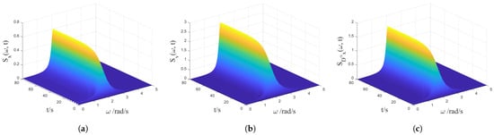
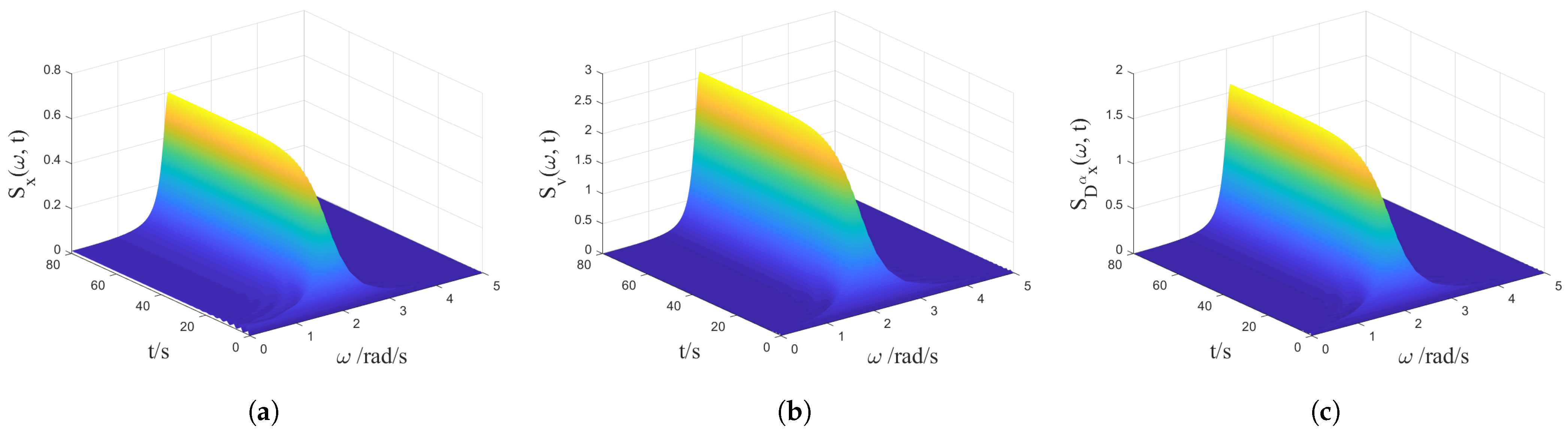
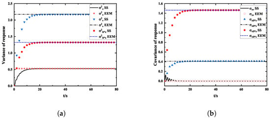
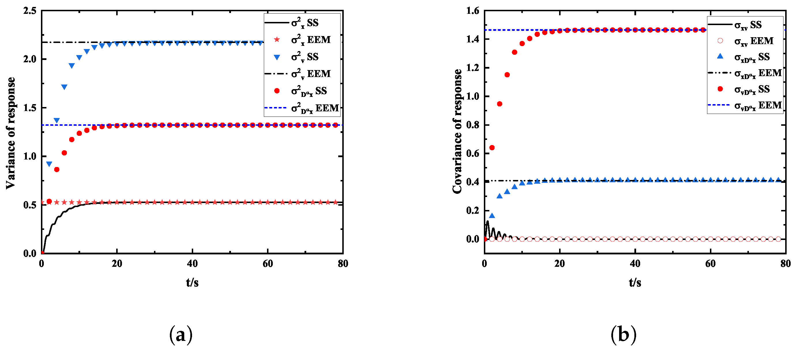
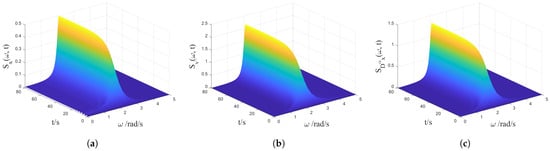
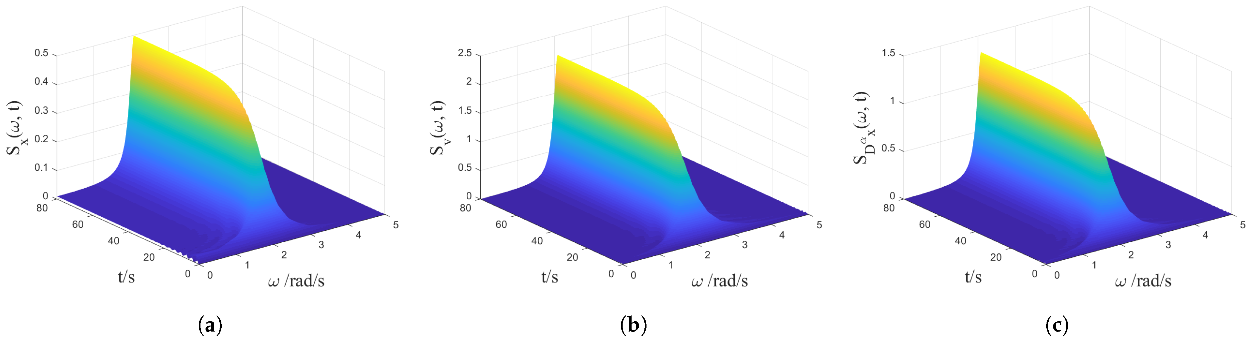
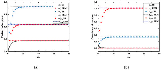
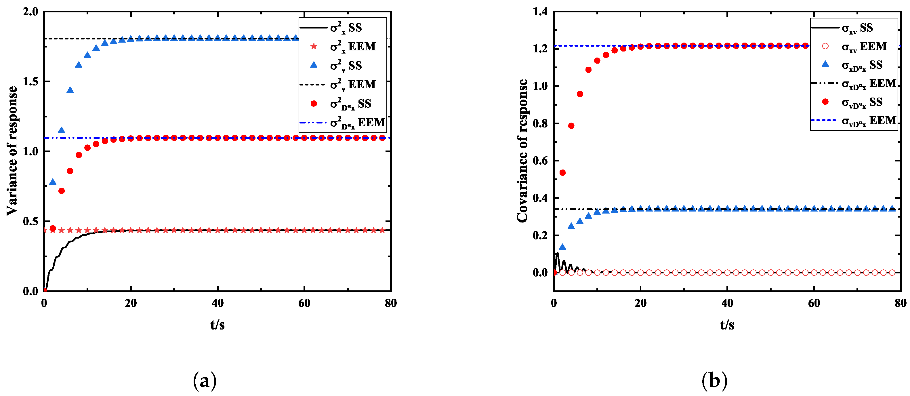
In the case where , the excitation becomes exponential noise. The system parameters are , , and . The excitation parameters are and . Based on the closed-form solution of , the time–frequency plot of the response PSD is illustrated in Figure 1. The curve representing the variation of the system’s response variance over time can be obtained by integration in the frequency domain. The variances and covariances of the displacement, velocity, and fractional derivative term are shown in Figure 2a and b, respectively. The results obtained using the eigenvector expansion method (EEM) are compared with the steady-state solution (SS) obtained from Monte Carlo (MC) simulations. The response for each sample in the MC simulations is computed using the predictor–corrector method. The time step is s, and the number of samples is 5000. The variances and covariances increase rapidly during the initial stage, indicating that the excitation energy injected into the system progressively amplifies the response fluctuations. Owing to the influence of fractional-order damping, the variance and covariance eventually stabilize, signifying that the system response has reached a steady state. The EEM results exhibit good agreement with the MC results. The temporal evolutions of the displacement, velocity, and fractional derivative variances are generally consistent, although they differ in their steady-state amplitudes and convergence rates. The displacement variance, which characterizes the dispersion of the vibration amplitude, evolves in comparatively gradually. The velocity variance is more sensitive to the high-frequency components of random excitation, and it directly reflects the rate of change of the system state. It can be seen in Figure 2b that the steady-state covariances and are non-zero, indicating that the fractional derivative term is correlated with both the displacement and velocity. Nevertheless, the covariance between displacement and velocity is zero, indicating that they are uncorrelated.
Figure 1.
Response PSDs of an SDOF linear oscillator with fractional derivatives when , obtained using the closed-form solution: (a) PSD of the displacement; (b) PSD of the velocity; (c) PSD of the fractional derivative term.
Figure 2.
Responses of an SDOF linear oscillator with fractional derivatives when , obtained from MC simulations and the EEM: (a) response variances of the displacement, velocity, and fractional-order term; (b) response covariances of the displacement, velocity, and fractional-order term.
Similar results are shown in Figure 3 and Figure 4 for . The other parameters are consistent with those previously described. The noise sample in the MC simulations can be obtained by employing a second-order linear filter on the Gaussian white noise. The variance and covariance curves rapidly increase during the initial stage and quickly stabilize due to the effect of damping. This indicates that the system response has reached a steady state. A subsequent comparison of the EEM results and the MC results reveals perfect agreement.
Figure 3.
Response PSDs of an SDOF linear oscillator with fractional derivatives when , obtained using the closed-form solution: (a) PSD of the displacement; (b) PSD of the velocity; (c) PSD of the fractional derivative term.
Figure 4.
Responses of an SDOF linear oscillator with a fractional-order viscoelastic damper when , obtained from MC simulations and the EEM: (a) response variances of the displacement, velocity, and fractional-order term; (b) response covariances of the displacement, velocity, and fractional-order term.
3.2. A 2-DOF Linear System with Fractional Derivatives
Consider a two-degree-of-freedom shear-type system with fractional-order viscoelastic terms. The equations of motion are
where are the mass, stiffness, and fractional-order damping coefficients; are related orders; and denotes exponential cosine colored noise.
Equation (78) can be rewritten in matrix form as
where , , , .
It is evident that the base order is , and the number of state variable matrices is .
By introducing the vector of the state variables
Equation (79) can be rewritten as
where , , and .
By performing eigenvector expansion and complex modal transformation, the set of decoupled fractional differential equations is obtained
Similarly, the PSD of the velocity can be obtained using the following equations
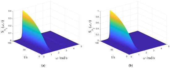
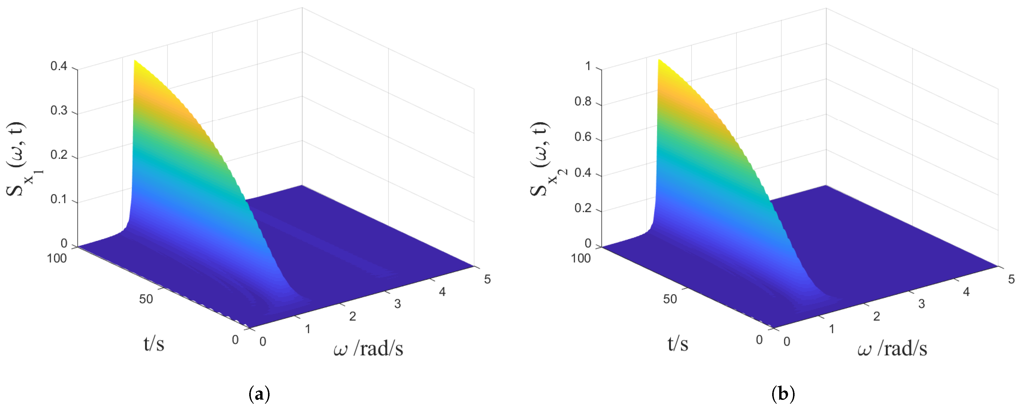
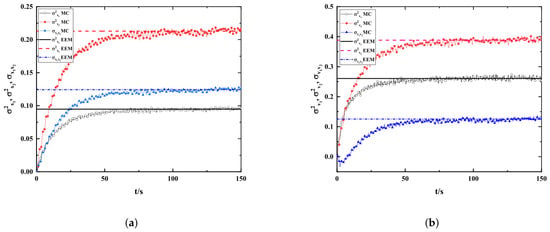
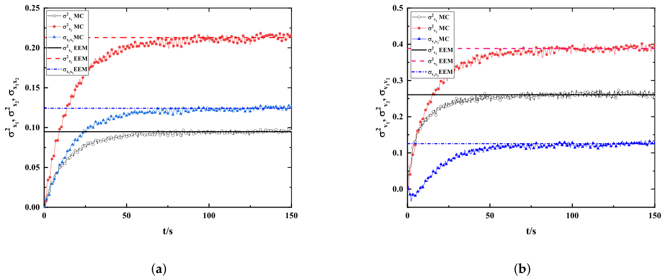
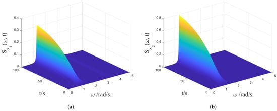
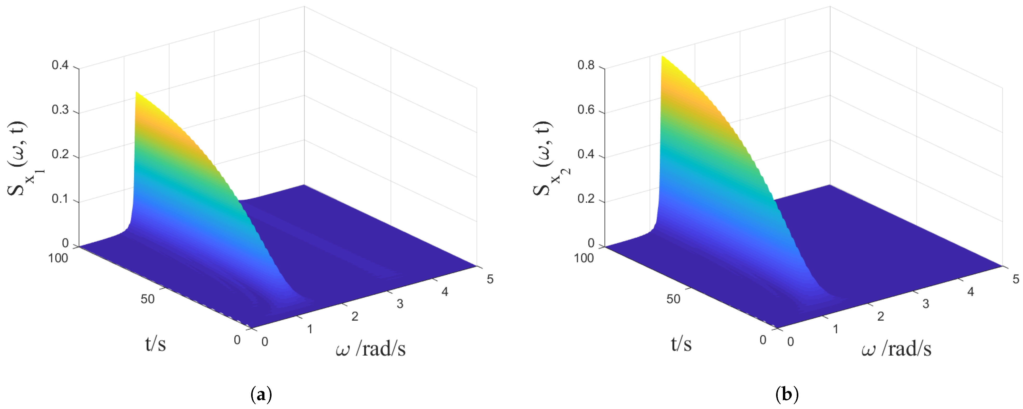
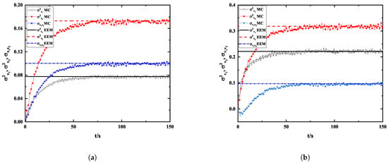
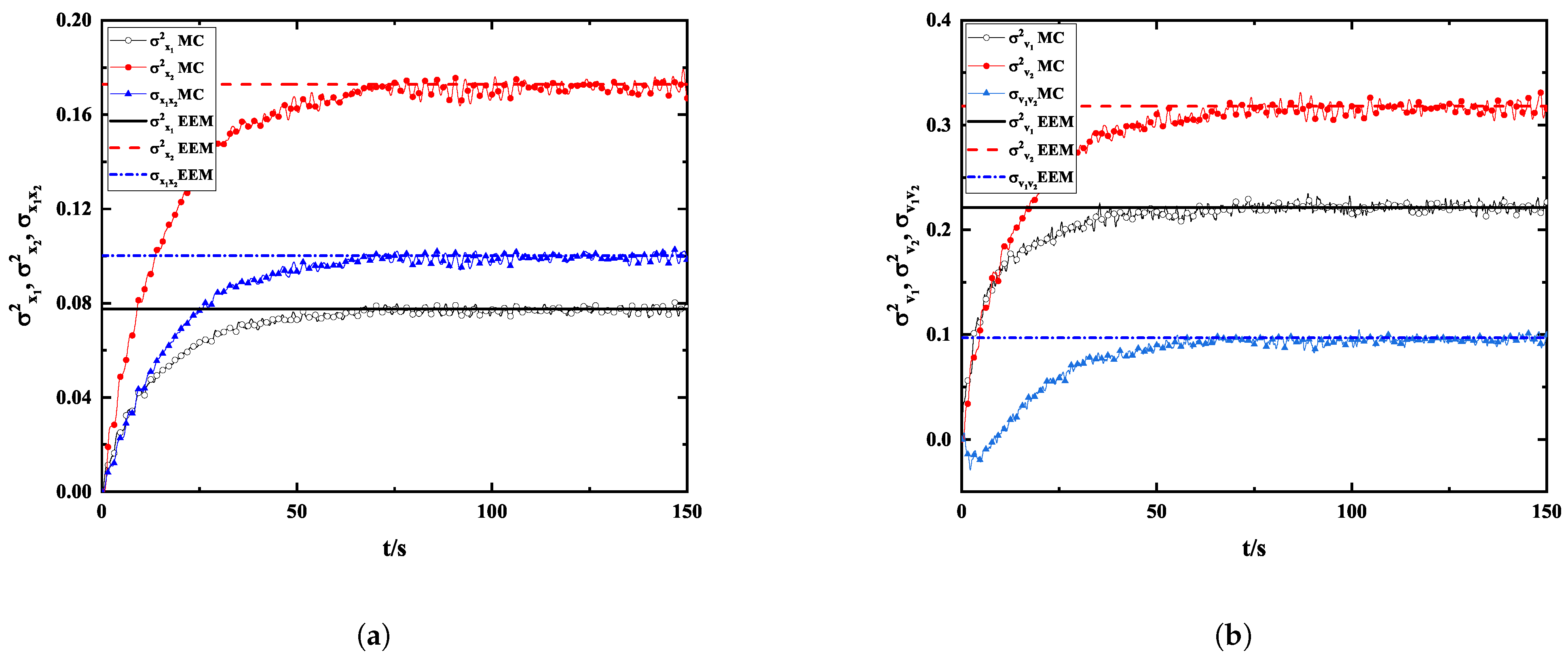
Assuming that , it is obvious that . Consider the case when ; in this instance, the excitation is exponential noise. The system parameters are , , , and . The excitation parameters are and . In the MC simulations, the time step is s, and the number of samples is 5000. The time–frequency plot of the displacement PSD obtained using the closed-form solution is shown in Figure 5. The time–frequency displacement PSD is integrated over frequency to yield the variance time history, from which the steady-state value is taken and compared with the Monte Carlo results. The statistics of the displacement , , and are shown in Figure 6a. It can be seen in the MC simulation curves that in the initial 50 s, the displacement variance increases rapidly with time, indicating the continuous application of input excitation energy. This results in the gradual augmentation of random fluctuations in the response. After 50 s, the rate of increase gradually decreases, and the variance fluctuates around a certain constant value, indicating that the system response has reached a steady state. The EEM results align closely with the MC results. The displacement variance of the first DOF is smaller than that of the second DOF. Figure 6b shows the curves of the velocity response statistics. The variation trend is consistent with that of the displacement response. However, a discrepancy is observed in the steady-state amplitude. The statistical values of the velocity are larger than those of the displacement since the velocity variance is more sensitive to the high-frequency components of the random excitation.
Figure 5.
Displacement PSDs of a 2-DOF linear oscillator with fractional derivatives when , obtained using the EEM: (a) PSD of the first DOF; (b) PSD of the second DOF.
Figure 6.
Responses of a 2-DOF linear oscillator with fractional derivatives when , obtained from MC simulations and the EEM: (a) statistics of displacement; (b) statistics of velocity.
The displacement PSDs are shown in Figure 7 and the statistics of the displacement and velocity responses when are shown in Figure 8. The parameters are consistent with those previously described. The trend of the statistics curves is consistent with those in Figure 6, exhibiting a rapid increase during the initial stage, followed by fluctuations around a certain value. However, the steady-state amplitudes of the case when are smaller than those in Figure 6. The variances of the displacement and velocity for the second DOF exhibit a greater magnitude than those observed for the first DOF. The values of the velocity variance are greater than those of the displacement variance. All curves show that the results of the EEM are in good agreement with the steady-state values of the MC simulations.
Figure 7.
Displacement PSDs of the 2-DOF linear oscillator with fractional derivatives when , obtained using the EEM: (a) PSD of the first DOF; (b) PSD of the second DOF.
Figure 8.
Responses of a 2-DOF linear oscillator with fractional derivatives when , obtained from MC simulations and the EEM: (a) statistics of the displacement; (b) statistics of the velocity.
3.3. An SDOF Fractional System with Cubic-Plus-Quintic Stiffness
Consider an SDOF system with fractional-order damping and cubic-plus-quintic stiffness. The equation of motion is
where , and k are the coefficients for mass, fractional-order damping, and stiffness, respectively. and are parameters denoting the nonlinear strength, and f represents colored noise, which is generated by the following first-order filter equation:
where denotes zero-mean Gaussian white noise with a constant PSD and is the parameter of the filter. In fact, it is easy to verify that the spectral density function is given by
and when takes a large value.
The nonlinear stiffness term is
The equation for the difference between the equivalent system and the original system is
According the criterion of minimum mean-square deviation of equations, we have
The equivalent stiffness coefficient is derived as follows:
The potential energies of the original system and the equivalent system are
and
The difference in potential energy between the two systems is
According to the criterion of minimum mean-square deviation of dissipative energy, we have
The equivalent stiffness coefficient can be derived as
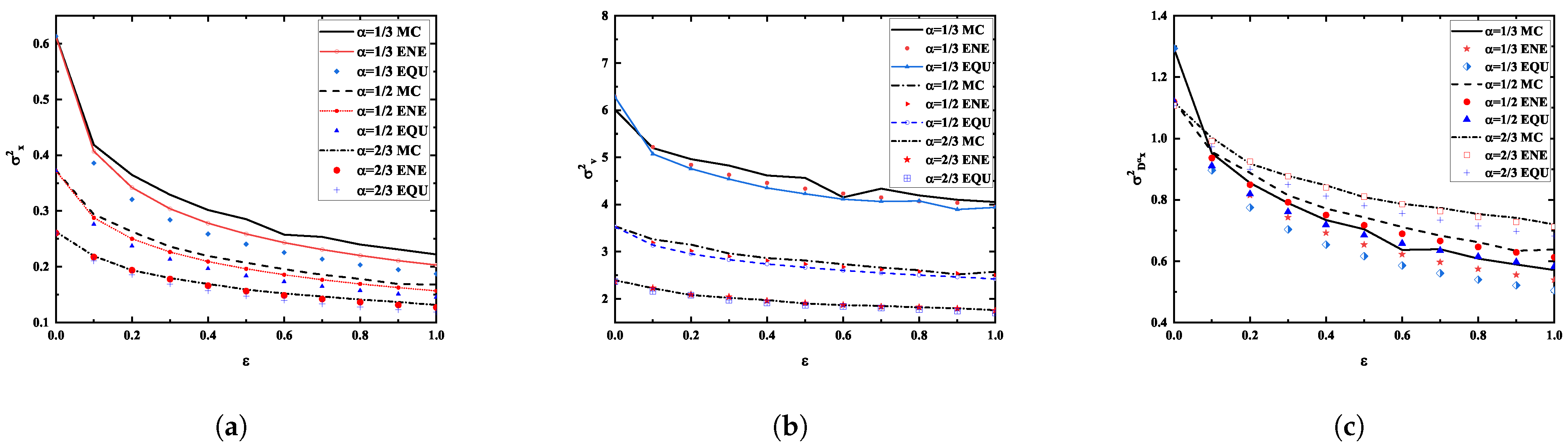
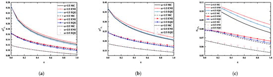
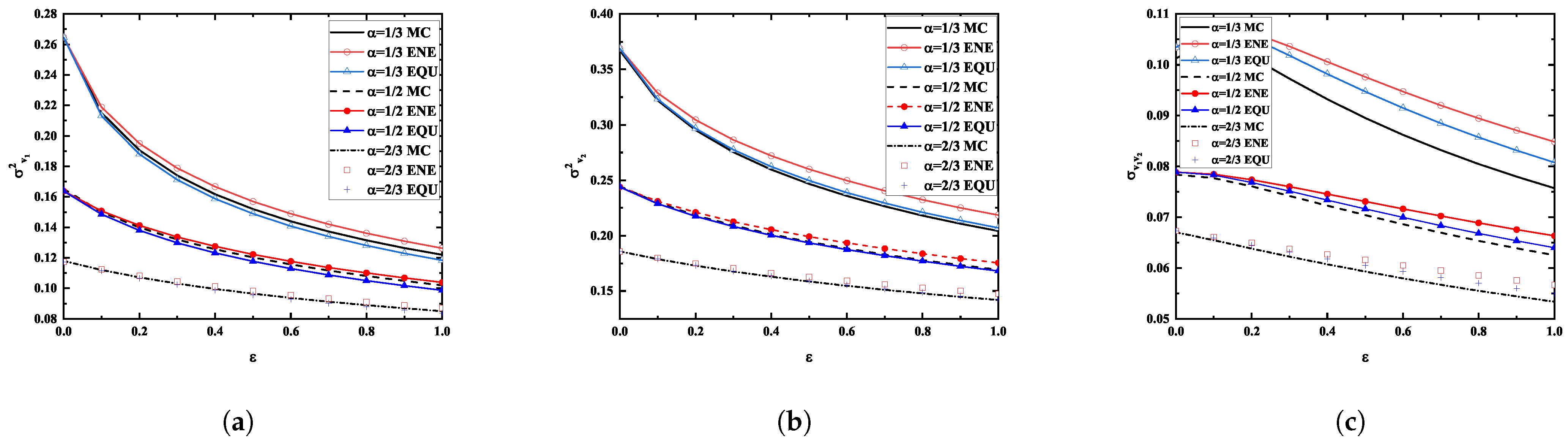
First, the effects of nonlinear strength and the order of the fractional derivative on the response variance are investigated. The system parameters are , , , , , , and . In the MC simulations, the sample number is 500, and the time step is s. The curves of the system’s steady-state variance of the displacement, velocity, and fractional derivative term versus the nonlinearity intensity for are shown in Figure 9. It can be seen that the variances of the response (including displacement, velocity, and fractional derivative term) decrease as the nonlinearity enhances for different orders. The variances of the displacement and velocity actually decrease as the order of the fractional operator increases. This phenomenon can be attributed to the inherent properties of fractional operators, which exhibit both stiffness and damping. As the order increases, the stiffness decreases while the damping capacity increases at the same time. This indicates that the changes in order can influence the memory and energy dissipation characteristics of the system, resulting in a significant moderating effect on the system’s stochastic response. The results obtained using the ELM are lower than those obtained from the MC simulations. Concurrently, it is evident that the results of the ELM based on the energy (ENE) difference criterion are closer to the MC results than those based on the equation (EQU) difference criterion. The maximum error associated with the ENE criterion is , whereas the maximum error for the EQU criterion is 15.79%.
Figure 9.
Response variance versus nonlinear strength: (a) displacement variance; (b) velocity variance; (c) fractional derivative variance.
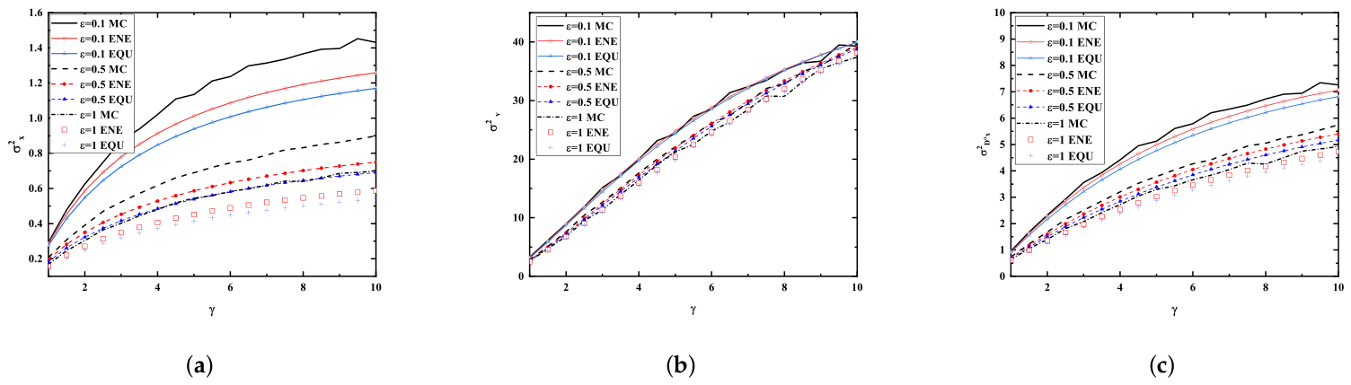
In Figure 10, the influence of the filter parameter on the response variance is investigated. The parameters in this example are , , , , , and . As the parameter increases, the displacement variance gradually increases. This is due to the fact that an increase in raises the PSD of the colored noise according to Equation (92), which in turn amplifies the energy of the input excitation and ultimately leads to a greater degree of response dispersion. The variances of the velocity and the fractional derivative term exhibit the same trend. In the context of different nonlinear conditions, the trend of the displacement variance with respect to remains consistent. In circumstances where the system exhibits strong nonlinearity, the response variance is reduced. This phenomenon can be attributed to the enhancement of the system’s restoring force and resistance to deformation brought on by the elevated nonlinear stiffness. The enhanced stiffness can also improve the system’s dynamic stability and effectively suppress the amplitude of stochastic response, which is consistent with the conclusion presented in Figure 9. Compared with the response variances obtained from the MC simulations, the results obtained using the equivalent linearization method exhibit close agreement, demonstrating the effectiveness of the method in determining the stochastic responses of nonlinear fractional-order systems subjected to colored noise. It can also be seen that the results of linearization based on the energy (ENE) difference criterion are more accurate than those of linearization based on the equation (EQU) difference criterion.
Figure 10.
Response variance versus filter parameter : (a) displacement variance; (b) velocity variance; (c) fractional derivative variance.
3.4. A 2-DOF Fractional-Order System with Cubic Damping and Cubic Stiffness
Consider an additional 2-DOF nonlinear system with cubic damping and cubic stiffness endowed with fractional elements, where the stochastic excitation is applied only to mass . The dynamic equations that govern the system are expressed as
where are the mass, stiffness, and fractional-order damping coefficients; are the related orders; is the nonlinear strength; and represents exponential cosine colored noise.
After performing the following transformation:
and rewriting Equation (102) in matrix form as
where , , , , the nonlinear force is written as
and the excitation is written as
By substituting Equation (105) into Equations (13), (19) and (24), the equivalent stiffness and damping coefficients of the two linearization criteria can be derived as
and
The equivalent stiffness and damping coefficients can be rewritten in matrix form as
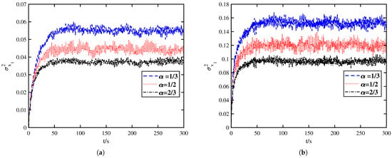
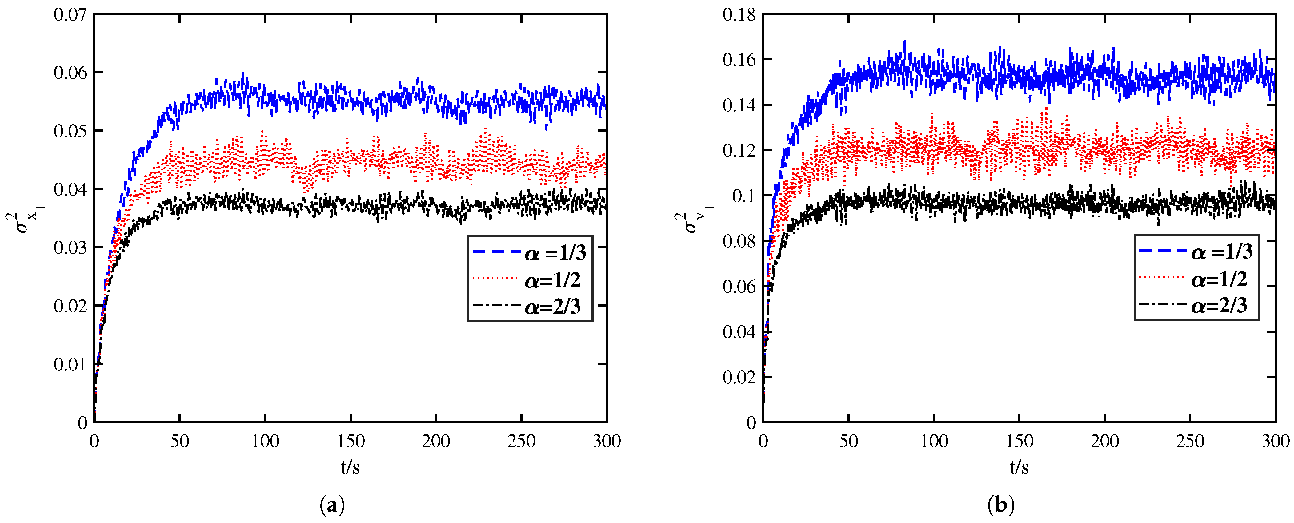
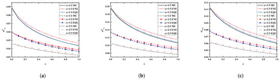
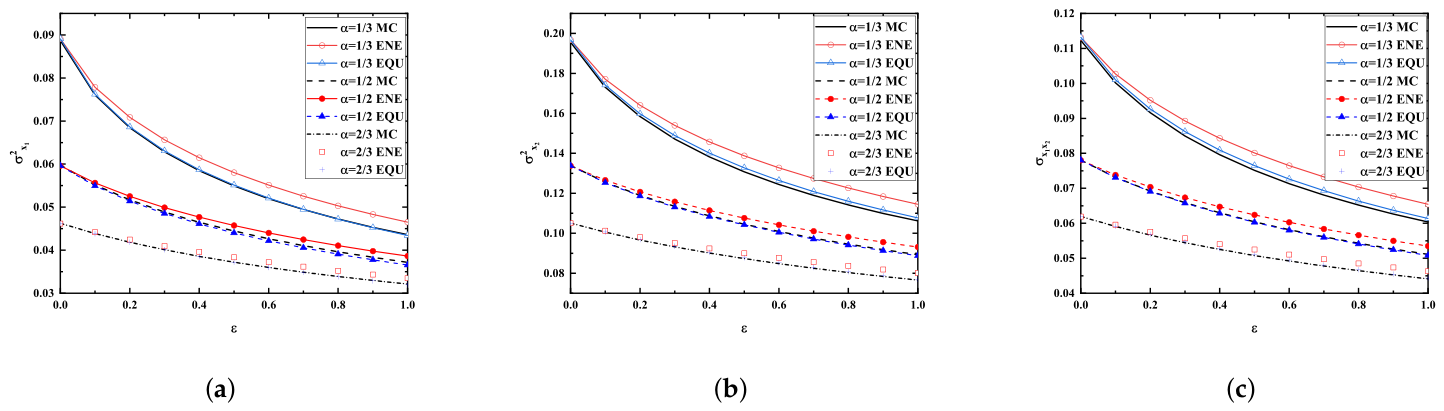
In this section, colored noise–exponential noise () with a double-sided PSD is considered. The parameters are , , , , , , and . In the MC simulations, the sample number is , the time step is s, and the total simulation time is T = 300 s. As shown in Figure 11, the time-domain curves of the response variance of the first DOF are depicted when . Figure 12 shows the system’s displacement variance and covariance versus nonlinear strength. It can be observed that as the nonlinearity improves, the variance and covariance exhibit a decreasing trend. This decline is attributed to the fact that stronger nonlinearity enhances the effective damping and stiffness of the system. The increased damping dissipates more energy, thereby suppressing the random vibration response. Meanwhile, the elevated stiffness provides greater restraint against external excitation. Collectively, these effects serve to reduce the dispersion of the displacement response. As the order of the fractional derivative increases, the displacement variance and covariance decrease.
Figure 11.
Response variances of the first DOF in the MC simulations when : (a) displacement variance; (b) velocity variance.
Figure 12.
Statistics of displacement versus nonlinear strength : (a) displacement variance of the first DOF; (b) displacement variance of the second DOF; (c) covariance of the system displacement.
Compared with the steady-state displacement variance and covariance obtained from the MC simulations, the results obtained by both linearization criteria are in good agreement. The errors evaluated using the ENE criterion reach approximately in a few cases, while remaining below at the majority of points. In contrast, the errors obtained from the EQU criterion are consistently less than . These results demonstrate that, for the present numerical example, the EQU criterion delivers superior performance.
The statistics of the velocity response are shown in Figure 13. It is evident that the velocity variance undergoes a gradual decline as the nonlinearity increases. The velocity covariance also exhibits a similar trend, with the exception of a minor increase at . The magnitude of the velocity variance is greater than that of the displacement variance because the PSD of the velocity is more sensitive to high-frequency components. It is evident that as the order of the fractional derivative increases, the statistics of the velocity decrease. Compared with the steady-state velocity variance and covariance obtained from MC simulations, the results obtained using both linearization criteria are in good agreement. The errors evaluated using the ENE criterion reach approximately in the estimation of while remaining below at the majority of points. In contrast, the maximum error obtained from the EQU criterion is . These results demonstrate that the EQU criterion delivers superior performance in this example.
Figure 13.
Statistics of velocity versus nonlinear strength : (a) velocity variance of the first DOF; (b) velocity variance of the second DOF; (c) covariance of the system velocity.
3.5. A 5-DOF Duffing System with Fractional Derivatives
Consider a 5-DOF shear-type Duffing system with fractional derivatives excited by exponential colored noise. The equation of motion is
where are the mass, fractional-order damping, and stiffness matrix, respectively, and , and are the acceleration, displacement, and fractional derivative vector of the system, respectively. The relative displacement can be expressed as
The nonlinear restoring force is rewritten as
and the equivalent form from the ELM is expressed as
where the equivalent stiffness coefficients using the EQU and ENE criteria are
and
where .
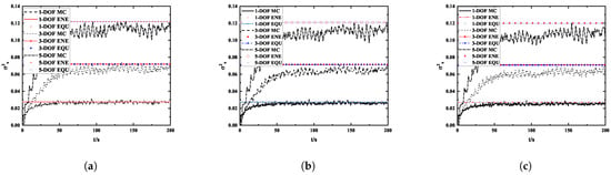
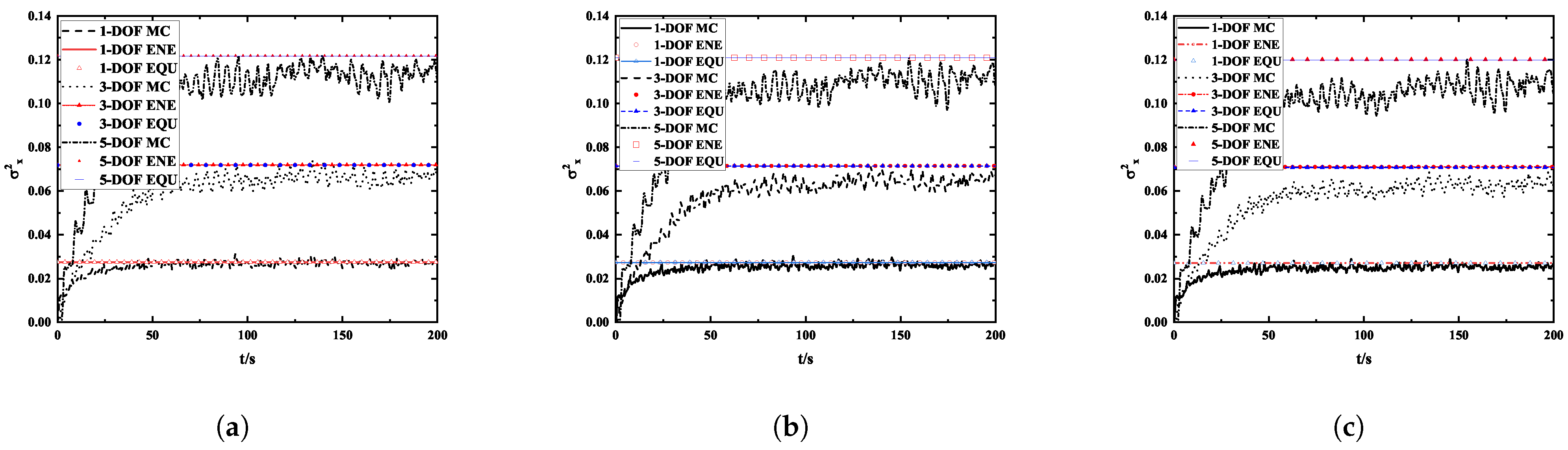
Assume that the parameters for all degrees of freedom are the same: , , , and . The colored noise only acts upon the first DOF, while the excitations on the other DOF are zero. The parameters for excitation are , . The number of samples in the MC simulations is 1000 and the calculation time is set to 200 s in order to guarantee that the system response reaches a steady state. The displacement variance curves for the first, third, and fifth degrees of freedom with nonlinear strength are shown in Figure 14. When , the errors from the ENE criterion are and , respectively, while those from the EQU criterion are and , respectively. When , the errors from the ENE criterion are and , respectively, while those from the EQU criterion are and , respectively. The errors from the ENE criterion are and , respectively, while those from the EQU criterion are and , respectively, when . It is evident that the results obtained from the two linearization criteria (ENE and EQU) are in close agreement, and both exhibit satisfactory accuracy compared with the Monte Carlo solutions. However, as the nonlinear strength increases, the error associated with the ELM gradually grows. This degradation in accuracy can be attributed to the increasingly strong nonlinear effects in the system, which cause the dynamic response to deviate substantially from a Gaussian distribution. This limitation underscores the inherent constraint of the method when applied to strongly nonlinear systems. The Monte Carlo simulations took 3166.7 s, whereas the equivalent linearization methods using two criteria converged in merely 12 and 15 iterations for , respectively, taking only 5.027 s and 6.065 s. It is imperative to consider both efficiency and accuracy in selecting a computational method. For systems with weak to moderate nonlinearity, the equivalent linearization method therefore represents a highly suitable choice, as it achieves a favorable balance between acceptable accuracy and significantly reduced computational cost. In such regimes, the nonlinear effects are not severe enough to fundamentally violate the Gaussian assumption underlying linearization, thereby allowing the method to deliver reliable response statistics at a fraction of the cost of Monte Carlo simulations.
Figure 14.
Displacement variance of the 5-DOF fractional Duffing system with different nonlinear strengths: (a) ; (b) ; (c) .
4. Conclusions
In this paper, the stochastic responses of MDOF linear/nonlinear systems with rational-order fractional derivatives subjected to colored noise are determined. By combining the eigenvector expansion method with a pole-residue representation of the system’s transfer function, a closed-form analytical expression for the PSDs of MDOF linear systems with fractional derivatives under colored noise is derived. By integrating the PSD over the frequency range, second-order statistical moments, such as variance and covariance, are obtained in a computationally efficient manner. Within an ELM framework, the original nonlinear fractional-order system is replaced with an equivalent linear system whose parameters are determined by minimizing the mean-square deviation between the two systems. During the iterative procedure, the response statistics of the linear system are obtained through eigenvector expansion and complex variable analysis. Two widely adopted linearization criteria—the energy-based criterion, which minimizes the mean-square difference of potential and dissipative energy, and the equation-based criterion, which minimizes the mean-square difference of the governing equation—are examined. Linear examples, including an SDOF linear system with fractional derivatives and a 2-DOF fractional-order linear system subjected to exponential-cosine colored noise, are presented to verify the efficiency of the EEM. Nonlinear examples, including an SDOF fractional-order system with cubic-quintic stiffness, a 2-DOF fractional-order system with cubic stiffness and damping, and a 5-DOF fractional-order Duffing system subjected to colored noise, are used to verify the accuracy of the equivalent linearization technique. A comparison with Monte Carlo simulations reveals that, for SDOF systems, the results obtained using the energy-based linearization criterion are more accurate than those derived using the equation-based criterion. For MDOF systems, both criteria demonstrate high accuracy and significantly lower computational costs. It is crucial to take into account the balance between computational accuracy and efficiency when selecting a method. It is also observed that the equation-based criterion yields slightly superior results compared with the energy-based criterion for MDOF systems. This contrasting behavior can be partly explained by the observation that in SDOF systems, the energy-based measure effectively captures the global balance of potential and dissipative energy, which governs the overall response. In MDOF systems, the equation-based criterion enforces stricter point-wise satisfaction of the governing equations, usually leading to improved accuracy when multiple interacting degrees of freedom are present, particularly in the case of viscoelastic damping with long-memory characteristics. The effects of the order of fractional derivatives and the nonlinear strength on response statistics are also investigated.
It should be noted that, in addition to the Monte Carlo method, the equivalent linearization method remains the most widely adopted approach for determining the stochastic response of nonlinear systems. In this regard, further research could focus on stochastic analysis of complex excitations, such as nonstationary and non-Gaussian, or multi-correlated stochastic excitations. Additionally, complex fractional-order systems, such as variable-order fractional-order systems, in which the order can vary with time, temperature, and other environmental conditions, pose enormous challenges in modeling and computation. Investigating how to adapt the ELM framework to handle such systems and improve the accuracy of the ELM is meaningful and promising for further development.
Author Contributions
Conceptualization, W.S. and J.G.; methodology, W.S. and X.K.; software, W.S.; data curation, W.S.; validation, W.S.; writing, W.S.; review and editing, J.G. and X.K.; supervision, X.K.; funding acquisition, J.G. and X.K. All authors have read and agreed to the published version of the manuscript.
Funding
This research received no external funding.
Data Availability Statement
The original contributions presented in this study are included in the article. Further inquiries can be directed to the corresponding author.
Conflicts of Interest
The authors declare no conflicts of interest.
References
- Bagley, R.L.; Torvik, P.J. Fractional calculus-a different approach to the analysis of viscoelastically damped structures. AIAA J. 1983, 21, 741–748. [Google Scholar] [CrossRef] [Scilit]
- Dong, Y.; Han, Y.; Zhang, Z. On the analysis of nonlinear dynamic behavior of an isolation system with irrational restoring force and fractional damping. Acta Mech. 2019, 230, 2563–2579. [Google Scholar] [CrossRef] [Scilit]
- Li, H.; Xu, Z.; Gomez, D.; Gai, P.; Wang, F.; Dyke, S.J. A modified fractional-order derivative zener model for rubber-like devices for structural control. J. Eng. Mech. 2022, 148, 04021119. [Google Scholar] [CrossRef] [Scilit]
- Lewandowski, R.; Pawlak, Z. Response spectrum method for building structures with viscoelastic dampers described by fractional derivatives. Eng. Struct. 2018, 171, 1017–1026. [Google Scholar] [CrossRef] [Scilit]
- Xu, J.; Li, J. Stochastic dynamic response and reliability assessment of controlled structures with fractional derivative model of viscoelastic dampers. Mech. Syst. Signal Process. 2016, 72, 865–896. [Google Scholar] [CrossRef] [Scilit]
- Barone, G.; Di Paola, M.; Iacono, F.L.; Navarra, G. Viscoelastic bearings with fractional constitutive law for fractional tuned mass dampers. J. Sound Vib. 2015, 344, 18–27. [Google Scholar] [CrossRef] [Scilit]
- Dai, J.; Xu, Z.D.; Gai, P.P.; Li, H.W. Effect of frequency dependence of large mass ratio viscoelastic tuned mass damper on seismic performance of structures. Soil Dyn. Earthq. Eng. 2020, 130, 105998. [Google Scholar] [CrossRef] [Scilit]
- Spanos, P.; Zeldin, B. Random vibration of systems with frequency-dependent parameters or fractional derivatives. J. Eng. Mech. 1997, 123, 290–292. [Google Scholar] [CrossRef] [Scilit]
- Denoël, V. Multiple timescale spectral analysis of a linear fractional viscoelastic system under colored excitation. Probabilistic Eng. Mech. 2018, 53, 66–74. [Google Scholar] [CrossRef] [Scilit]
- Ye, K.; Li, L.; Tang, J. Stochastic seismic response of structures with added viscoelastic dampers modeled by fractional derivative. Earthq. Eng. Eng. Vib. 2003, 2, 133–139. [Google Scholar] [CrossRef] [Scilit]
- Huang, Z.; Jin, X.; Lim, C.W.; Wang, Y. Statistical analysis for stochastic systems including fractional derivatives. Nonlinear Dyn. 2010, 59, 339–349. [Google Scholar]
- Cao, Q.; Hu, S.L.J.; Li, H. Nonstationary response statistics of fractional oscillators to evolutionary stochastic excitation. Commun. Nonlinear Sci. Numer. Simul. 2021, 103, 105962. [Google Scholar] [CrossRef] [Scilit]
- Kong, F.; Xu, Y.; Ding, Z.; Sun, X. Analytical nonstationary response of linear stochastic MDOF systems endowed with half-order fractional derivative elements. ASCE-ASME J. Risk Uncertain. Eng. Syst. Part A Civ. Eng. 2024, 10, 04023048. [Google Scholar] [CrossRef] [Scilit]
- Pinnola, F.P. Statistical correlation of fractional oscillator response by complex spectral moments and state variable expansion. Commun. Nonlinear Sci. Numer. Simul. 2016, 39, 343–359. [Google Scholar] [CrossRef] [Scilit]
- Pirrotta, A.; Kougioumtzoglou, I.; Di Matteo, A.; Fragkoulis, V.; Pantelous, A.; Adam, C. Deterministic and random vibration of linear systems with singular parameter matrices and fractional derivative terms. J. Eng. Mech. 2021, 147, 04021031. [Google Scholar] [CrossRef] [Scilit]
- Di Matteo, A.; Spanos, P.D. Determination of nonstationary stochastic response of linear oscillators with fractional derivative elements of rational order. J. Appl. Mech. 2024, 91, 041008. [Google Scholar]
- Xu, Y.; Kong, F.; Hong, X.; Hu, Z.; Ding, Z. Analytical non-stationary response of fractional linear systems endowed with arbitrary rational order fractional derivative elements and subject to evolutionary stochastic excitation. Mech. Syst. Signal Process. 2025, 226, 112333. [Google Scholar] [CrossRef] [Scilit]
- Di Paola, M.; Failla, G.; Pirrotta, A. Stationary and non-stationary stochastic response of linear fractional viscoelastic systems. Probabilistic Eng. Mech. 2012, 28, 85–90. [Google Scholar] [CrossRef] [Scilit]
- Su, C.; Xian, J. Nonstationary random vibration analysis of fractionally-damped systems by numerical explicit time-domain method. Probabilistic Eng. Mech. 2022, 68, 103228. [Google Scholar] [CrossRef] [Scilit]
- Chen, L.; Wang, W.; Li, Z.; Zhu, W. Stationary response of Duffing oscillator with hardening stiffness and fractional derivative. Int. J. Non-Linear Mech. 2013, 48, 44–50. [Google Scholar] [CrossRef] [Scilit]
- Chen, E.; Xing, W.; Wang, M.; Ma, W.; Chang, Y. Study on chaos of nonlinear suspension system with fractional-order derivative under random excitation. Chaos Solitons Fractals 2021, 152, 111300. [Google Scholar] [CrossRef] [Scilit]
- Guan, Y.; Li, W.; Kozak, D.; Zhao, J. Response and reliability analysis of a nonlinear VEH systems with FOPID controller by improved stochastic averaging method and LBFNN algorithm. Reliab. Eng. Syst. Saf. 2024, 249, 110206. [Google Scholar] [CrossRef] [Scilit]
- Spanos, P.D.; Evangelatos, G.I. Response of a non-linear system with restoring forces governed by fractional derivatives—Time domain simulation and statistical linearization solution. Soil Dyn. Earthq. Eng. 2010, 30, 811–821. [Google Scholar] [CrossRef] [Scilit]
- Spanos, P.D.; Zhang, W. Nonstationary stochastic response determination of nonlinear oscillators endowed with fractional derivatives. Int. J. Non-Linear Mech. 2022, 146, 104170. [Google Scholar] [CrossRef] [Scilit]
- Xu, Y.; Kong, F.; David, D.; Hong, X.; Sun, X. Non-stationary response determination of nonlinear systems endowed with fractional derivative elements subjected to evolutionary stochastic excitation. Eng. Struct. 2024, 319, 118844. [Google Scholar] [CrossRef] [Scilit]
- Zhang, W.; Spanos, P.D.; Di Matteo, A. Nonstationary stochastic response of hysteretic systems endowed with fractional derivative elements. J. Appl. Mech. 2023, 90, 061011. [Google Scholar] [CrossRef] [Scilit]
- Zhao, N.; Wang, X.; Wu, Y. Nonstationary random vibration analysis of hysteretic systems with fractional derivatives by FFT-based frequency domain method. Mech. Syst. Signal Process. 2024, 220, 111666. [Google Scholar] [CrossRef] [Scilit]
- Xian, J.; Su, C. Nonstationary random vibration analysis of fractionally-damped nonlinear systems by equivalent linearization based on explicit time-domain method. Reliab. Eng. Syst. Saf. 2025, 264, 111452. [Google Scholar] [CrossRef] [Scilit]
- Di Matteo, A.; Spanos, P.; Pirrotta, A. Approximate survival probability determination of hysteretic systems with fractional derivative elements. Probabilistic Eng. Mech. 2018, 54, 138–146. [Google Scholar] [CrossRef] [Scilit]
- Kougioumtzoglou, I.A.; Ni, P.; Mitseas, I.P.; Fragkoulis, V.C.; Beer, M. An approximate stochastic dynamics approach for design spectrum based response analysis of nonlinear structural systems with fractional derivative elements. Int. J. Non-Linear Mech. 2022, 146, 104178. [Google Scholar] [CrossRef] [Scilit]
- Zhang, Y.; Li, S.; Kong, F. Survival probability of nonlinear oscillators endowed with fractional derivative element and subjected to evolutionary excitation: A stochastic averaging treatment with path integral concepts. Probabilistic Eng. Mech. 2021, 66, 103156. [Google Scholar] [CrossRef] [Scilit]
- Fragkoulis, V.C.; Kougioumtzoglou, I.A. Survival probability determination of nonlinear oscillators with fractional derivative elements under evolutionary stochastic excitation. Probabilistic Eng. Mech. 2023, 71, 103411. [Google Scholar] [CrossRef] [Scilit]
- Spanos, P.D.; Pomaro, B. Stochastic response spectrum determination of nonlinear systems endowed with fractional derivative elements. Nonlinear Dyn. 2025, 113, 14791. [Google Scholar] [CrossRef] [Scilit]
- Zhang, Y.; Li, S.; Zhu, Z.; Fragkoulis, V.C. Approximate response determination of nonlinear oscillators with fractional derivative elements subjected to combined periodic and evolutionary stochastic excitations. Mech. Syst. Signal Process. 2025, 229, 112485. [Google Scholar] [CrossRef] [Scilit]
- Kong, F.; Zhang, H.; Zhang, Y.; Chao, P.; He, W. Stationary response determination of MDOF fractional nonlinear systems subjected to combined colored noise and periodic excitation. Commun. Nonlinear Sci. Numer. Simul. 2022, 110, 106392. [Google Scholar] [CrossRef] [Scilit]
- Kong, F.; Han, R.; Zhang, Y. Approximate stochastic response of hysteretic system with fractional element and subjected to combined stochastic and periodic excitation. Nonlinear Dyn. 2022, 107, 375–390. [Google Scholar]
- Zhang, Y.; Han, R.; Zhang, P. Stochastic response of chain-like hysteretic MDOF systems endowed with fractional derivative elements and subjected to combined stochastic and periodic excitation. Acta Mech. 2024, 235, 5019–5039. [Google Scholar] [CrossRef] [Scilit]
- Di Matteo, A. Response of nonlinear oscillators with fractional derivative elements under evolutionary stochastic excitations: A Path Integral approach based on Laplace’s method of integration. Probabilistic Eng. Mech. 2023, 71, 103402. [Google Scholar] [CrossRef] [Scilit]
Disclaimer/Publisher’s Note: The statements, opinions and data contained in all publications are solely those of the individual author(s) and contributor(s) and not of MDPI and/or the editor(s). MDPI and/or the editor(s) disclaim responsibility for any injury to people or property resulting from any ideas, methods, instructions or products referred to in the content. |
© 2026 by the authors. Licensee MDPI, Basel, Switzerland. This article is an open access article distributed under the terms and conditions of the Creative Commons Attribution (CC BY) license.