Flutter Analysis of Telescopic Wing Structures Based on Non-Matching Grid Contact Equivalence

Abstract

The frequency-domain flutter analysis method requires a linear model as input; however, when a telescopic actuator is applied to morphing aircraft, traditional frequency-domain flutter analysis methods face challenges in addressing issues involving contact nonlinearity. To enable classical frequency-domain methods to handle this type of nonlinearity, this paper presents an equivalent linearization modeling method for morphing aircraft wing structures. The proposed modeling method uses rod elements as the equivalent linearization elements and avoids the need to handle node correspondence issues. The model is parameterized by the rod element’s elastic modulus, contact surface distance, and element length coefficient. Upon completion of the equivalent modeling, flutter analysis can be performed by the PK method. The proposed modeling method increases modeling efficiency while maintaining the accuracy of the model. A simulation study of a typical hypersonic telescopic wing structure is conducted. The effects of angle of attack and altitude on flutter characteristics are analyzed. The proposed modeling method effectively captures both the static and dynamic characteristics of the original structure. The flutter Mach number decreases with increasing extension length, and it increases with altitude and angle of attack. The flutter frequency decreases with increasing extension length, angle of attack, and altitude.

1. Introduction

Morphing aircraft offer significant advantages in achieving global aerodynamic optimization compared to fixed-wing aircraft [1,2,3,4,5,6,7]. A telescopic spanwise-extending wing is an aircraft structure that morphs via translational motion in the lateral direction, with the morphing process actuated by telescopic actuators. This type of aircraft structure exhibits distinct aerodynamic characteristics under different extension states. Moreover, as the wing extends, the interaction between the wing and the telescopic actuators also varies accordingly, resulting in non-unique contact states. The telescopic actuator is an essential structural component used to constrain and drive the wings [8]. However, conventional flutter analysis methods rely on linear models as input to establish flutter equations in the frequency domain and cannot analyze models with complex contact interactions. Therefore, time-domain methods are often employed to solve models that involve contact [9,10,11].

Wing flutter is a typical dynamic aeroelastic phenomenon [12,13,14,15,16,17]. It is a self-excited and potentially destructive oscillation that can lead to catastrophic failure of the aircraft [18,19,20,21]. During the flutter process, the aerodynamic forces exhibit periodic variation characteristics [22,23,24]. Extensive studies on aerodynamic loads have also been conducted by numerous researchers. During the wing deformation process, the flutter boundary evolves accordingly, resulting in a flight envelope that is no longer fixed, but rather a function of the wing deformation parameters. Xie et al. [25] proposed an innovative interpolation method for the coupling relationship between structural and aerodynamic models. Yan et al. [26] studied active flutter suppression in variable flaps, demonstrating that variant designs can improve wing flutter performance with higher control efficiency and smaller amplitude. Xie et al. [27] investigated supersonic flutter mechanisms for “diamond-back” folding wings, analyzing flutter characteristics during deformation using reduced-order aerodynamic models. Despite these advancements, current flutter analyses for morphing wing aircraft primarily use CFD or reduced-order models. However, a notable deficiency remains in aeroelastic research specifically focusing on wings equipped with telescopic actuators. Addressing this deficiency requires the development of an equivalent linearization method tailored for flutter analysis.

The telescopic wing is driven by an integrated telescoping mechanism to achieve wing deformation [8]. The telescopic actuator is a conventional driving mechanism with a nested configuration, where the internal cavity generates thrust through high-pressure gas to achieve telescoping motion. This structure is capable of withstanding normal forces, while friction in the tangential direction remains minimal, ensuring smooth movement. To analyze the flutter characteristics under varying telescoping states, equivalent linearization must be applied to the contact region. Thin-layer elements are commonly used for equivalent linear modeling of structures with relatively fixed contact surface positions. By appropriately selecting thin-layer element material parameters, the contact mechanical characteristics can be equivalently modeled [28,29,30,31,32]. Rimpel [33] employed thin-layer elements to simulate reduced stiffness at the axial contact surface of rod rotors. Liu et al. [34] proposed a new semi-analytical method for nonlinear analysis. Li and Yuan [35] applied thin-layer elements for equivalent modeling of rod rotor contact surfaces. Du et al. [36] exploited virtual material methods based on three-dimensional fractal contact theory to study rod rotor contact characteristics. Compared to contact algorithms, the thin-layer element method linearizes contact, improving computational and analytical efficiency. Existing contact equivalent linearization methods require node matching between two contact surfaces [37]. The motion of the telescopic actuator causes changes in the contact region, and when the thin-layer element method is used for equivalent linearization modeling, it is crucial to ensure that the mesh in the contact region matches. Therefore, modeling for multiple telescoping states necessitates repeated mesh adjustments, making traditional thin-layer element-based equivalent modeling methods unsuitable. These processes lead to decreased efficiency. The principal novelty of the proposed method lies in performing equivalent linearization modeling based on rod elements. In contrast to approaches such as the thin-layer element method and the virtual material method, linearization modeling using rod elements enables a point-to-point treatment of the finite element model, obviating the need for separate adjustments to different contact states. This feature allows the establishment of a highly versatile equivalent modeling procedure, capable of batch-generating equivalent linearized models for various contact states. Upon completion of the equivalent linearization modeling, static characteristic analysis (a surface pressure load is applied to one side of the wing skin to simulate the aerodynamic forces acting on the wing, and the structural deformation characteristics are obtained by solving the static equilibrium equations) can be performed, followed by dynamic characteristic analysis (which analyzes the modal parameters of the structure).

The frequency-domain flutter analysis method requires the model to be linear, excluding any nonlinear factors (such as contact nonlinearity). This requirement imposes limitations on modeling structures with contact, particularly for morphing wings, where the contact surfaces may change [9,10,11]. To address the applicability issue of frequency-domain flutter analysis methods for wing models with contact nonlinearities, this paper proposes an equivalent modeling method based on rod elements, which serves as an auxiliary approach to extend the application scope of these methods. The parameters for equivalent modeling are identified using particle swarm optimization (PSO) [38]. Subsequently, flutter analysis is conducted based on the equivalent model. A simulation study is performed on a typical telescopic wing structure. The results show that this equivalent modeling method accurately captures the static and dynamic characteristics of the original model. Flutter analysis is performed under varying conditions. The results reveal the variation patterns of flutter boundaries with altitude and angle of attack for the telescopic wing. This method improves modeling efficiency while maintaining accuracy. It provides a novel approach for flutter analysis of wings with contact nonlinearity.

2. Flutter Analysis Method Based on Non-Matching Grid Contact Equivalence

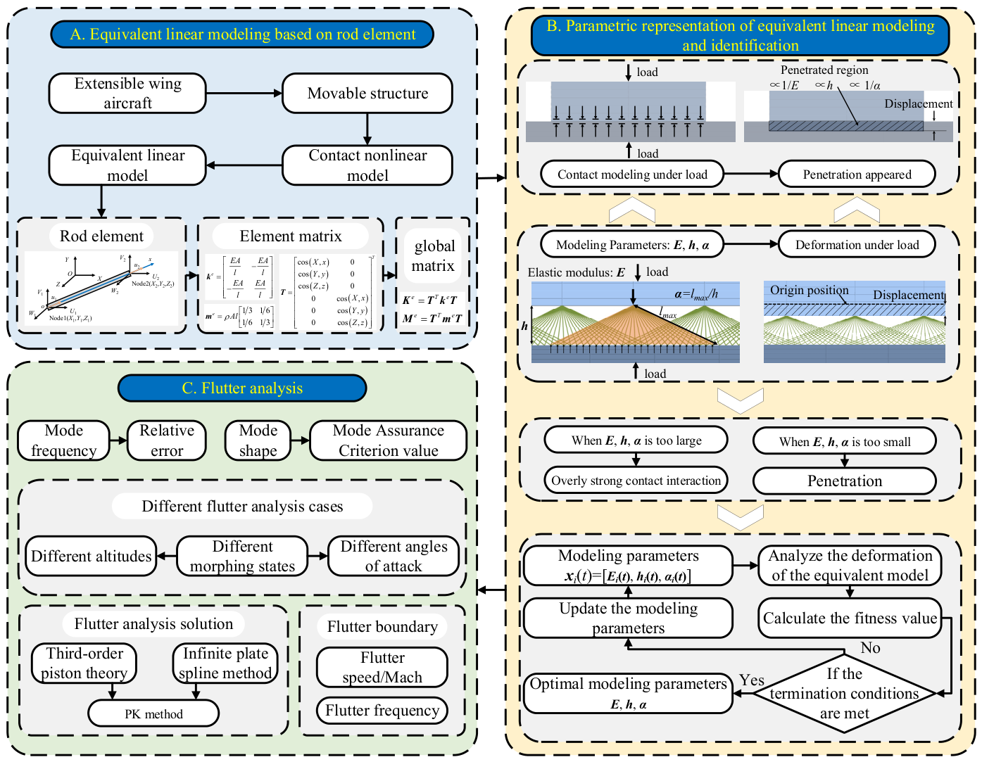
This section introduces the method used for flutter analysis of models with contact nonlinearity. First, based on the mechanical characteristics of planar contact surfaces, a contact nonlinear model is constructed. Subsequently, equivalent linearization operations are performed based on this model, leading to an equivalent linearization modeling method and providing the theoretical foundation. The equivalent contact element is represented using rod elements. The point-to-point characteristic of the rod element eliminates the need for node matching. Next, the methods for parametric characterization and parameter identification are introduced. Finally, it provides the approach for verifying dynamic accuracy and the steps for performing flutter analysis under different morphing states. This section is shown in Figure 1.

2.1. Equivalent Linear Modeling Based on Rod Element

The contact surfaces only bear out-of-plane normal forces, and the in-plane frictional forces are negligible. The equivalent modeling needs to characterize the constraint effect on the deformation of the airfoil in the normal direction. The structural form of the equivalent modeling is shown in Figure 1A. Between the planar sliding contact surfaces, contact transmits normal pressure without transferring bending moments. Rod elements only transmit axial forces and do not transfer bending moments, making them more suitable than beam elements for equivalent linearization. Hence, rod elements are used to connect the nodes in the contact region between the planar sliding contact surfaces. Additionally, the transmission of contact forces should occur between corresponding positions on the contact surfaces. For two nodes on the contact surfaces, the more perpendicular the rod element connecting the two nodes, the better it can transmit normal pressure. Conversely, the ability to transmit normal pressure is reduced. It is important to note that the rod element significantly increases the in-plane stiffness, but this has minimal effect on the flutter boundary. This is because in the actual flight state, the aerodynamic force of the wing only exists in the normal direction with almost no in-plane load. The first-order mode of wing structure primarily involves normal (bending) deformation, and thus the transverse stiffness component introduced by the rod elements exerts only a limited influence on this mode. The second-order mode, on the other hand, corresponds to torsional deformation. However, in the actual process of torsional deformation, the telescopic actuator is housed within the sleeve associated with the wing, and there exists a fit constraint between the actuator and the wing such that the two components essentially undergo synchronous torsion. Consequently, the rod elements experience relatively small forces, and their effect on the dynamic characteristics is likewise minor. Therefore, regardless of the presence of in-plane stiffness, the in-plane response is nearly zero. In summary, using rod elements for connection offers advantages. It better characterizes the constraint effect of the telescopic actuator.

Compared to traditional thin layer elements, the modeling method proposed in this paper avoids the need for node correspondence. Additionally, when different relative positions of the two contact surfaces are analyzed, the corresponding parts of the original model can be directly moved. Equivalent contact elements can be then established. This simplifies the modeling process.

The equivalent elements are chosen as first-order rod elements. The linear interpolation method is employed to calculate the internal displacement of the elements, from which strain and stress are subsequently derived. Consider a first-order rod element in the global coordinate system OXYZ, with a total length l, a cross-sectional area A and an elastic modulus E. A local one-dimensional coordinate system ox is established. The x-axis coincides with the rod element’s axis, the origin is at Node 1, and the positive direction of the x-axis points towards Node 2. In this local coordinate system, the element stiffness matrix k^e in the local coordinate system based on the principle of virtual work is given by Equation (1) [39]:

$${\mathit{k}}^e=\left[\begin{array}{cc}{\displaystyle \frac{EA}{l}}& -{\displaystyle \frac{EA}{l}}\\ -{\displaystyle \frac{EA}{l}}& {\displaystyle \frac{EA}{l}}\end{array}\right]$$

(1)

The element mass matrix m^e in the local coordinate system is given by Equation (2) [39]:

$${\mathit{m}}^e=\rho Al\left[\begin{array}{cc}1/3& 1/6\\ 1/6& 1/3\end{array}\right]$$

(2)

where ρ is the material density.

For the element stiffness matrix K^e and the element mass matrix M^e in the global coordinate system OXYZ, a coordinate transformation method is required to convert the matrices from the local coordinate system into the global coordinate system. The element stiffness matrix and mass matrix in the global coordinate system are as follows [39]:

$$\begin{array}{l}{\mathit{K}}^e={\mathit{T}}^T{\mathit{k}}^e\mathit{T}\\ {\mathit{M}}^e={\mathit{T}}^T{\mathit{m}}^e\mathit{T}\end{array}$$

(3)

where T is the coordinate transformation matrix.

The stiffness matrices and mass matrices of the elements are integrated into the global matrices to achieve equivalent contact modeling in the analysis.

2.2. Parametric Representation of Equivalent Linear Modeling and Identification

The equivalent modeling parameterization and parameter identification are shown in Figure 1B. The modeling method uses the elastic modulus E of rod elements, the contact surface distance h, and the element length coefficient α as parameterized characterization parameters:

Elastic modulus E: The elastic modulus significantly impacts the contact force transmission characteristics. If the elastic modulus is too small, the relative displacement between the two contact surfaces will be large, resulting in a phenomenon similar to contact surface penetration. Conversely, if the elastic modulus is too large, the constraint effect on the structure will be too strong, making it difficult to accurately reflect the deformation.

Contact surface distance h: The distance h between the contact surfaces is crucial for characterizing contact performance. h directly affects the inclination of the rod elements, thereby influencing the normal pressure transmission. If h is too small, the rod elements will be unable to effectively transmit contact forces. Conversely, the forces in the non-contact area will become excessively strong.

Element length coefficient α: This coefficient controls the generation of rod elements. A rod element is generated only if its length l satisfies l ≤ αh. If α is too small, there will be insufficient rod elements to transmit enough contact force. Conversely, if α is too large, the contact forces will be excessively strong.

The results of the nonlinear contact model analysis serve as the basis for parameter identification. In finite element theory, the primary quantity is the node displacement. Other quantities are derived from displacement and material parameters. Therefore, displacement is used as the characterization parameter.

Select the region with significant structural deformation as the area of focus. Assemble the three-directional displacements in sequence into a vector u_exact for the original model. The original model refers to a nonlinear model constructed by defining the contact relationships between the contact surfaces, where contact algorithms are used to analyze the structural mechanical properties. It does not incorporate any equivalent linearization and provides the most accurate results. Similarly, assemble the vector u_equal for the equivalent model. Perform a correlation analysis between these two vectors and define the fitness function as shown in Equation (4):

$$F\left(E,h,\alpha \right)={\displaystyle \frac{{\mathit{u}}_{exact}\cdot {\mathit{u}}_{equal}}{\left|{\mathit{u}}_{exact}\right|\cdot \left|{\mathit{u}}_{equal}\right|}}$$

(4)

The fitness function F (E, h, α) ranges from [−1, 1]. A value of 1 indicates the highest similarity between the two vectors. Therefore, the optimization goal is to select F (E, h, α) approaching 1.

The PSO algorithm [38] is employed to identify the equivalent modeling parameters. This method employs random particles to simulate the foraging behavior of bird flocks, continuously searching in the optimization space. All particles share information and adjust their velocity direction based on search results, gradually approaching the optimal target. The PSO algorithm has advantages such as fast convergence speed and good robustness. These advantages make it more suitable for identifying equivalent modeling parameters than other optimization algorithms.

The velocity update equation for the PSO algorithm is shown in Equation (5), and the parameters update equation is shown in Equation (6):

$$\begin{array}{l}{\mathit{v}}_i\left(t+1\right)=\omega {\mathit{v}}_i\left(t\right)+c_1{r}_1\left[{\mathit{x}}_{pbesti}-{\mathit{x}}_i\left(t\right)\right]\\ \hfill +c_2{r}_2\left[{\mathit{x}}_{gbest}-{\mathit{x}}_i\left(t\right)\right]\hfill \end{array}$$

(5)

$${\mathit{x}}_i\left(t+1\right)={\mathit{x}}_i\left(t\right)+{\mathit{v}}_i\left(t+1\right)$$

(6)

In the equations, v_i(t) and v_i(t + 1) represent the velocity vectors of particle i at time t and t + 1, respectively. x_i(t) and x_i(t + 1) are the modeling parameter vectors of particle i at time t and t + 1, respectively. ω is the inertia factor. c₁ is the cognitive factor. c₂ is the social factor. r₁ and r₂ are random numbers in the interval [0,1], which are used to increase the randomness of the search. x_pbesti is the personal best modeling parameter vector of particle i. x_gbest is the global best modeling parameter vector.

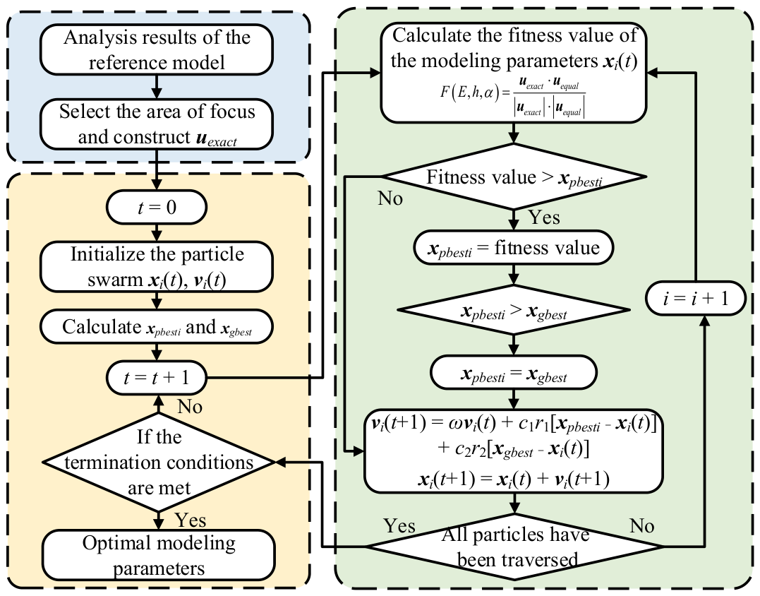
Given the influence of modeling parameters on the accuracy of static characteristic representation, the modeling parameters are identified based on the PSO algorithm. The flowchart of parameter identification is shown in Figure 2. The parameter identification procedure is as follows:

• Particle swarm initialization: Establish the contact equivalent finite element model. Construct a particle swarm of a certain size under given constraints. Randomly initialize all particle modeling parameter vectors, and velocity vectors, and set a limit on the number of iterations.
• Calculate fitness values: Calculate the fitness value of each particle based on the defined fitness function under the respective modeling parameter vectors.
• Update individual and global best modeling parameter vectors: Compare the fitness value of each particle with its individual best modeling parameter vector x_pbesti and the global best modeling parameter vector x_gbest. The better one is chosen to update x_gbest.
• Update individual position and velocity vectors: Based on x_i(t), v_i(t), x_pbesti, and x_gbest, calculate the velocity vector v_i(t + 1) and modeling parameter vector x_i(t + 1) for the next iteration.
• Check iteration termination conditions: If the termination conditions are met, stop the iteration. The global best position represents the optimization result. Otherwise, return to step 2.

2.3. Flutter Analysis Method

The flutter analysis process is shown in Figure 1C. Based on the identified parameters, equivalent linearization modeling is conducted. Subsequently, the accuracy of the equivalent model’s dynamic characteristics relative to the original model is validated. The dynamic characteristics include modal frequencies and modal shapes. The accuracy of modal frequencies is assessed using relative errors. The accuracy of modal shapes is evaluated using the Modal Assurance Criterion (MAC).

Based on the model with validated accuracy, flutter analysis is conducted. The aerodynamic theory employed is the third-order piston theory [40]. Interpolation between aerodynamic forces and structural motions is performed using the infinite plate spline theory [41]. The flutter solution method is the PK method [42]. Flutter analysis is carried out under various conditions to determine the variation patterns of structural flutter characteristics.

All flutter analyses in this paper are conducted within a linear framework, without considering the additional stiffness induced by geometric nonlinearity or the effects of static aeroelastic deformation. The aerodynamic stiffness effect, however, is taken into account in the flutter analysis. The analysis is based on the assumption of harmonic motion, and the aerodynamic forces also exhibit harmonic variation with a definite phase relationship relative to the structural motion. On this basis, the aerodynamic forces are represented by equivalent aerodynamic stiffness, aerodynamic damping, and aerodynamic mass, from which the flutter analysis equations are formulated and solved.

3. Numerical Simulation Study

This section introduces a flutter simulation study based on the equivalent linear modeling method, which is described in the previous section. A telescopic wing is constructed using the typical NACA0012 airfoil shape, with the wing beam incorporating a telescopic rod mechanism. Subsequently, the optimal modeling parameters are identified using the parameter identification method. The accuracy of the dynamic characteristics is then verified. Equivalent linearization models are established for different structural deformation states. Finally, flutter analysis is performed under various conditions, such as different angles of attack and different altitudes, resulting in the flutter boundaries.

3.1. Structural Model

The structural model is based on a telescopic wing with a NACA0012 airfoil shape. NACA0012 is a classic symmetrical airfoil, widely used in aircraft design and aerodynamic research. Analogous to the case presented in the reference, this type of wing structure is applied to unmanned aerial vehicles (UAVs) [8]. By adjusting the length of the wing in the airflow, flight performance can be modified, achieving a higher lift-to-drag ratio at low speeds and reduced drag at high speeds, thus realizing aerodynamic optimization across the entire flight envelope. This paper focuses on the wing structure, and therefore, the modeling and analysis are concentrated on the wing.

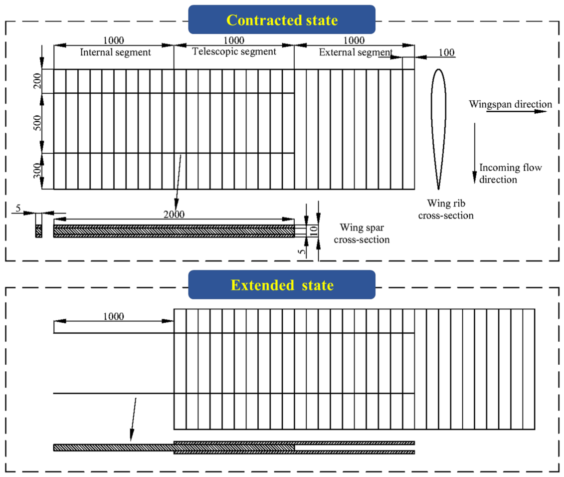
The wing has a span of 3000 mm, a chord length of 1000 mm, and a maximum thickness of 120 mm. The chordwise cross-sectional shape is symmetrical. In this model, the outer one-third of the wing is consistently positioned outside the fuselage, referred to as the external segment. The middle one-third constitutes the telescopic segment, which gradually extends from within the fuselage to the outside during the telescoping process. The inner one-third remains entirely within the fuselage, designated as the internal segment. The length of the wing axis outside the fuselage is referred to as the extension length. The schematic diagram of the structure shape and dimensions is shown in Figure 3, with dimensions in mm.

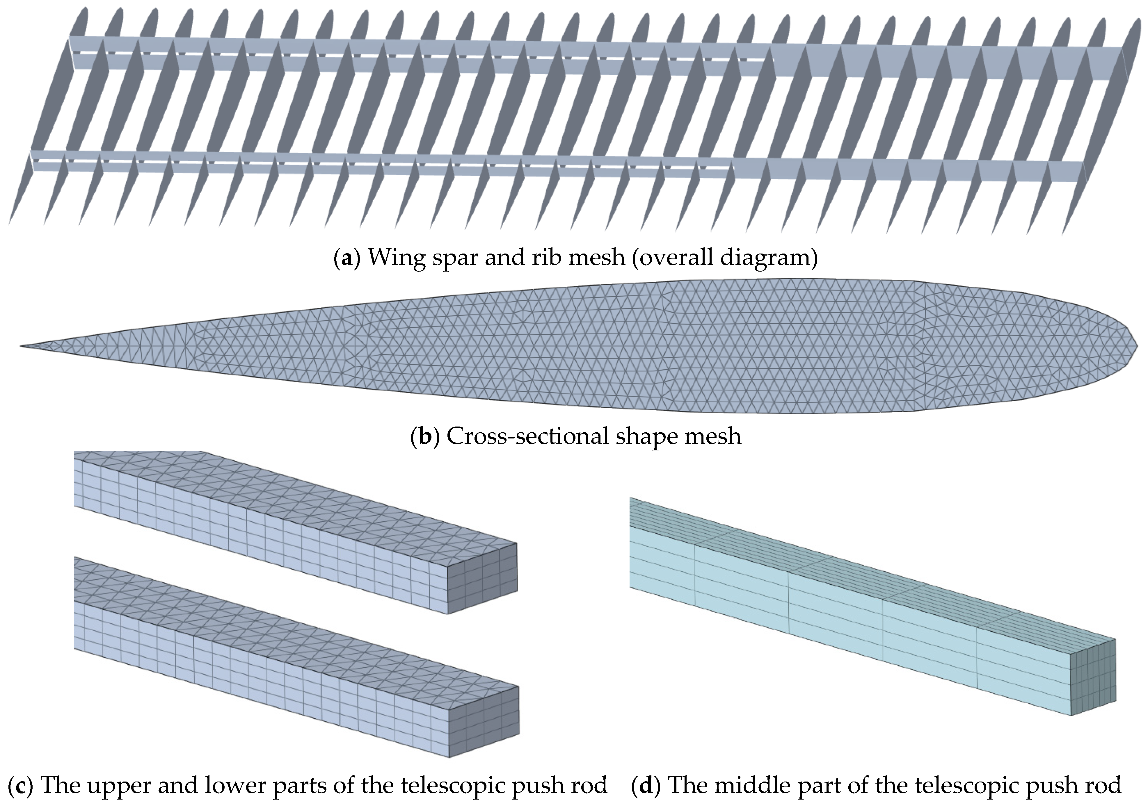
The skin, spars, and ribs, as shown in Figure 4a,b, are large-area structures with relatively small thickness, where the dimension in the thickness direction is significantly smaller than in the other directions. These components are thus typical thin-walled structures and can be simplified accordingly; consequently, shell elements are adopted for modeling. It should be noted that this simplified shell-element modeling approach is only applicable to structures exhibiting the aforementioned thin-walled characteristics. For the telescopic actuators, which exhibit slender-rod characteristics—namely, its dimension in the longitudinal direction is significantly larger than in the other directions—beam elements could be employed for simplified modeling. However, given that the present study focuses on the contact interface regions of this structure, solid elements are still adopted for modeling to ensure that the mechanical behavior of the contact surfaces can be adequately captured, as shown in Figure 4c,d. Regarding element type selection, the mesh of shell elements is generated using a hybrid combination of triangular and quadrilateral elements, while solid elements are discretized using a mix of hexahedral and triangular prism (wedge) elements. The total number of elements is 334,688, with 194,175 nodes. The upper and lower parts of the telescopic push rod are connected to the wing structure, while the middle part is fixed inside the fuselage. A contact relationship exists between the two, allowing sliding along the length direction, with a limiting device ensuring no lateral displacement. For modeling simplification, the limiting device is not modeled separately but is handled through degree-of-freedom constraints. The meshes between different parts of the telescopic actuators do not correspond, resulting in a non-matching mesh.

3.2. Aerodynamic Model

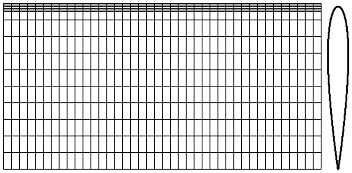
The aerodynamic mesh is shown in Figure 5, with the extended state used as an example. The spanwise direction is uniformly divided into 40 meshes, and the chordwise direction is divided into 15 meshes, totaling 600 meshes. The aerodynamic mesh is located on the symmetrical plane of the wing structure, and the spanwise grid size is determined based on the portion of the wing exposed to the airflow. To accurately reflect the shape characteristics of the airfoil, the mesh is denser at the front where the curvature is larger, and relatively sparser at the rear where the surface is flatter. Flutter analysis is performed based on the validated model, employing the third-order piston theory [40] for aerodynamic loads, the infinite plate spline method [41] for interpolation between aerodynamic forces and structural motions, and the PK method [42] for solving the flutter equation. The analysis is conducted under a variety of conditions to reveal the variation patterns of the structural flutter characteristics. In terms of the selection of aerodynamic theory, the third-order piston theory is an aerodynamic model applicable to high-speed flight regimes, with a validity range of Mach numbers from 4 to 20 [43,44]. Subsequent case studies indicate that the flutter Mach numbers fall within this range, and this theory has been widely adopted in flutter analysis [45]. In flutter analysis, other commonly used aerodynamic theories include the Doublet-Lattice Method (DLM), the Vortex Lattice Method (VLM), Computational Fluid Dynamics (CFD), and Reduced-Order Models (ROMs). The DLM is mostly employed for subsonic flutter analysis and is not suitable for the velocity regime of the present cases [46]. The VLM, based on potential flow theory, employs vortex rings to simulate the wing for aerodynamic load calculations and does not account for wing thickness effects [47]. The CFD approach directly solves the fluid and structural motion equations through a two-way fluid–structure interaction analysis, offering excellent accuracy, but its computational cost is considerably higher than that of frequency-domain aerodynamic methods [46,47]. The ROM approach requires training based on CFD results to establish the model, which also entails substantial preparatory effort [48,49]. Regarding airfoil compatibility, relevant studies have demonstrated that the piston theory is applicable to the NACA0012 airfoil used in the present cases [50]. In summary, the third-order piston theory is deemed appropriate for the cases investigated in this paper.

3.3. Equivalent Linearization Modeling

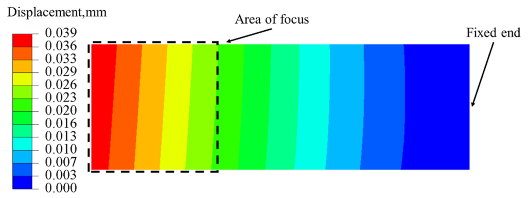
First, the structural mechanical behavior is analyzed using a contact algorithm. The contact is defined as normal hard contact with frictionless tangential interaction. For all extension states, the fully retracted state has the smallest aerodynamic force action area, and hence the aerodynamic contribution is relatively minor. At the same time, the contact area in the telescopic actuators region is the largest, resulting in a relatively greater contribution from contact interactions. As the wing gradually extends, the ratio of aerodynamic forces to contact interaction forces further increases, thereby reducing the error introduced by equivalent linearization modeling. By the same reasoning, for the dynamic characteristics of the structure, the stiffness and mass effects of the extended wing segment gradually become dominant as the wing extends. Therefore, the fully retracted state is selected for parameter identification in equivalent linearization modeling. Furthermore, modal characteristics depend on both stiffness and mass; stiffness is also reflected in static analysis, while mass is primarily governed by the extended wing segment. Consequently, parameter identification based on static analysis results can yield a satisfactory dynamic matching accuracy. This fully retracted state model is designated as the reference model. To simulate aerodynamic forces, a surface pressure load of 1 Pa is applied to the lower surface of the wing. The wing root is locked by a telescopic actuator, assumed to be a fixed support constraint. The analysis results of the reference model in the fully retracted state are shown in Figure 6. The results indicate that the wing portion exhibits typical deformation characteristics of a compressed cantilever beam. The external segment, enclosed by the dotted line, is selected as the focus area for calculating the fitness function of the equivalent model parameters.

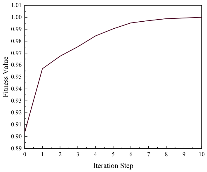
An equivalent linearization model is established based on the previously described method, and then the equivalent modeling parameters are identified. The identified parameters are E = 7412.85 MPa, h = 0.25 mm, and α = 4.14, with a fitness value of 0.999. The convergence curve of the iterative process is shown in Figure 7.

To evaluate the sensitivity of the equivalent model to parameter variations, a sensitivity analysis is conducted on the key parameters E, h, and α in the rod-element equivalent model. The analysis indicates that when E is sufficiently large, the normal pressure between contact interfaces can be effectively transmitted, with its specific value having little influence on the equivalent performance. The effective ranges of both h and α are relatively broad; issues such as insufficient or excessive connection stiffness only arise under extreme values. The equivalent performance remains satisfactory within α∈ [3,7], and even in a wider range, the performance exhibits only slight variations while remaining generally stable. Overall, the proposed equivalent model exhibits low sensitivity to parameter variations and demonstrates good robustness.

To verify the repeatability of the equivalent parameter identification, the particle swarm optimization algorithm is employed with a population size of 50 and 50 iterations. The search ranges are selected based on the following considerations: E is set within [10 MPa, 1000 GPa]; h is set within [0.05 mm, 1 mm], determined jointly by the mesh size of the contact region and the structural characteristic length—considering that the wing structure has a characteristic length on the order of meters, variations within this range have negligible impact on the overall mechanical performance—and α is set within [1,10], where the lower bound indicates that only exactly corresponding nodes generate rod elements, while the upper bound prevents unrealistically strong connections between non-corresponding nodes. The repeated optimization runs yielded the optimal parameter combination E = 7115.36 MPa, h = 0.16 mm, and α = 6.76, with a fitness value of 0.999. Compared with the parameter combination E = 7412.85 MPa, h = 0.25 mm, and α = 4.14, the decrease in h with a corresponding increase in α confirms the complementary relationship between the two parameters, further enhancing the consistency of the equivalent model across different parameter combinations.

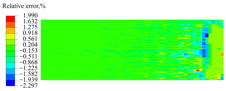
With the parameter combination E = 7412.85 MPa, h = 0.25 mm, and α = 4.14 as an example, the relative displacement error obtained from the equivalent model is shown in Figure 8, with the maximum absolute value of the relative error being 2.297%, indicating that the results are generally consistent with those in Figure 6. The primary sources of error can be attributed to three factors: (1) The contact calculation method ensures displacement continuity at the interface. However, in the equivalent contact model, the elastic deformation of the rod elements between the two contact surfaces leads to inconsistent displacements, resulting in slight penetration. The sufficient stiffness of the rod elements ensures that this penetration remains within an acceptable range. (2) The rod elements introduce transverse force components, but the directions of these forces vary between individual rod elements, and they essentially cancel each other out. (3) The rod elements impose constraints on the transverse movement of the structure, which differs from the assumption of frictionless tangential interaction. Nevertheless, since the load interface primarily carries normal forces, with negligible tangential forces, the presence of these constraints has minimal impact on the results. In conclusion, the three sources of error are well controlled, and thus the equivalent model accurately reflects the static characteristics of the reference model.

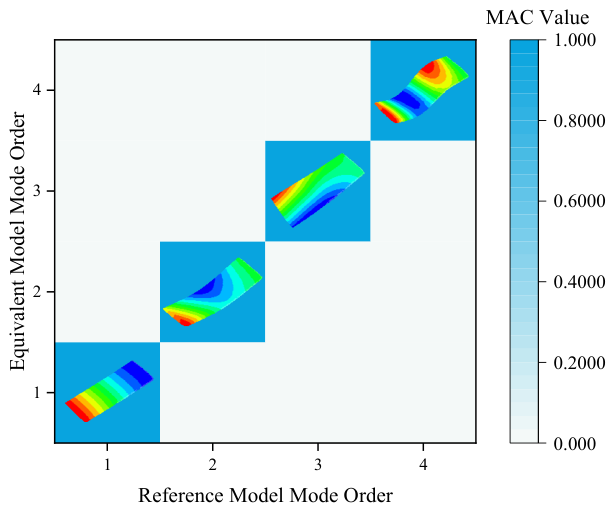
The accuracy of the dynamic characteristics primarily involves frequency and mode shapes. The comparison of frequency and mode shapes is shown in

Table 1. Comparison of frequencies for the 1000 mm extension state.

Mode Order	Reference Model	Equivalent Model	Relative Error
1	8.83 Hz	8.81 Hz	−0.23%
2	55.26 Hz	54.82 Hz	−0.80%
3	64.53 Hz	64.06 Hz	−0.73%
4	126.91 Hz	125.66 Hz	−0.98%

and Figure 9, demonstrating good agreement. The maximum absolute value of the relative frequency error is 0.98%. The minimum MAC value for the corresponding mode is 0.999, and the maximum MAC value for non-corresponding modes is 0.010. In the interest of conservatism, a zero damping assumption is adopted for all modes.

3.4. Flutter Analysis

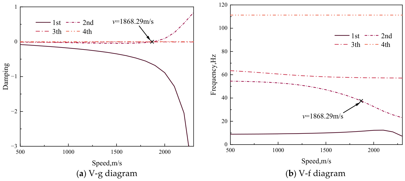
The simulation is performed for the 1000 mm state, at an altitude of 20 km [51] and an angle of attack of 0°. The V-g and V-f diagrams are shown in Figure 10. The flutter speed is 1868.29 m/s, the flutter Mach number is 6.33 Ma, and the flutter frequency is 37.50 Hz. The flutter mechanism involves the coupling of the first and second modes.

3.4.1. Analysis at Different Angles of Attack

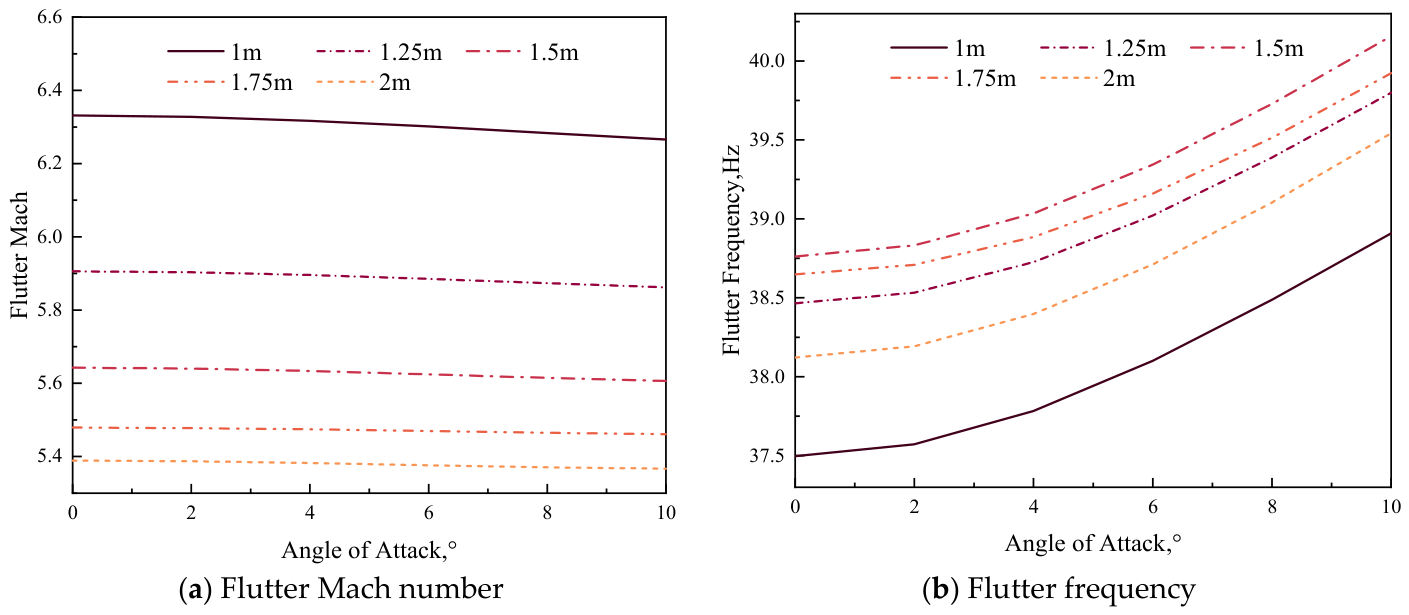
The simulation is performed for an angle of attack range of 0–10° [51], at an altitude of 20 km, and with extension lengths ranging from 1000 mm to 2000 mm in 250 mm intervals. The flutter Mach numbers and flutter frequencies are presented in Figure 11. The flutter Mach number decreases with increasing extension length and angle of attack. The highest flutter Mach number, 6.33 Ma, occurs at an extension length of 1000 mm and an angle of attack of 0°. The lowest flutter Mach number of 5.37 Ma is observed at 2000 mm extension length and 10° angle of attack. The flutter frequency increases as the angle of attack increases.

Under different angles of attack, the aerodynamic load distribution on the structure varies, which in turn influences the aerodynamic matrix terms in the flutter equation. Specifically, an increase in the angle of attack leads to a reduction in the aerodynamic damping term, while the ratio of aerodynamic stiffness to aerodynamic mass increases, resulting in a lower flutter speed and a higher flutter frequency.

3.4.2. Analysis at Different Altitudes

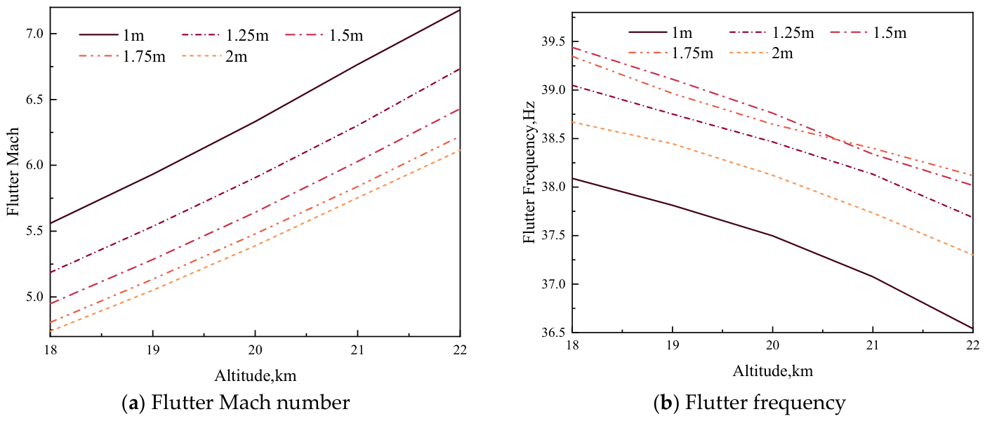
At altitudes between 18 and 22 km [51] with a 0° angle of attack, the flutter Mach number and flutter frequency are shown in Figure 12. The flutter Mach number increases with altitude, while the flutter frequency decreases with increasing altitude. The highest flutter Mach number of 7.18 Ma is observed at an extension length of 1000 mm and an altitude of 22 km. The lowest flutter Mach number of 4.74 Ma occurs at an extension length of 2000 mm and an altitude of 18 km. At different altitudes, the aerodynamic forces required for flutter are nearly constant. As altitude increases, the air density decreases, resulting in an increase in the flutter Mach number. Within the altitude range of 18 to 22 km, the speed of sound remains virtually constant. Consequently, the flutter Mach number follows a trend consistent with that of the flutter speed, increasing with altitude.

4. Conclusions

Existing frequency-domain flutter analysis methods have limitations. They cannot handle contact nonlinear models. To overcome these limitations, an equivalent modeling method is proposed in this study. The method utilizes rod elements and incorporates parameters such as the elastic modulus (E), contact surface distance (h), and element length coefficient (α) for parameterization. A parameter identification method is established based on the particle swarm optimization algorithm. Once the equivalent modeling is completed, flutter analysis can be conducted. A simulation study is conducted using a telescopic wing model to obtain flutter characteristics under various deformation states. The main conclusions are as follows:

• Under various deformation states, the equivalent model proposed in this paper accurately reflects the mechanical characteristics of the original structure. In the simulation study, the static characteristics match those of the reference model with a correlation of 0.999. The maximum absolute value of the relative frequency error is 0.98%, and the MAC values for the corresponding mode shapes all exceed 0.999.
• The equivalent modeling method proposed in this paper can efficiently handle variable contact surface conditions. Compared to traditional thin-layer element modeling methods, the proposed method avoids the issue of node matching on contact surfaces, ensuring both accuracy and improved efficiency.
• Flutter analysis can be successfully performed, indicating that the proposed method is efficient and accurate for flutter analysis of morphing wing aircraft with variable contact surfaces. Under different deformation states, based on the equivalent model, the simulation study is performed. The flutter Mach numbers and flutter frequencies under varying angles of attack and altitudes are obtained. The flutter Mach number decreases with increasing extension length, and it increases with altitude and angle of attack.

The method proposed in this paper has the following limitations: (1) the current method still relies on the quasi-static assumption and cannot account for the influence of deformation rate on flutter characteristics; and (2) there are limitations regarding the form of the contact surface. The method works well for planar and small-curvature contact surfaces, but it becomes cumbersome for contact surfaces with larger curvatures. This is because the contact surface needs to undergo small-scale movements to create space for the rod elements. For large-curvature surfaces, such operations often lead to severe deformations, deviating from the actual conditions. In the meantime, although the present study has been validated through simulation analyses, experimental verification has not yet been performed. Further research involving static, modal, or flutter tests is still required to validate the reliability of the proposed method.

The future research directions of this study can be considered from the following suggestions: (1) conduct ground tests, including static tests and modal tests, to validate the accuracy of the modeling approach; (2) carry out flutter flight tests, constructing a telescopic wing in a real flight environment, and further validate the method by studying the accuracy of the flutter boundary; (3) consider aerodynamic heating effects and study equivalent methods for heat transfer processes at the contact surfaces; (4) conduct contact equivalence studies for curved contact surfaces; and (5) focus on computational efficiency, constructing multi-layer rod-element structures based on the existing single-layer structure, and explore ways to further improve computational efficiency while ensuring accuracy.

References

1. Hammerton, J.R.; Su, W.; Zhu, G.; Swei, S.S. M: Optimum distributed wing shaping and control loads for highly flexible aircraft. Aerosp. Sci. Technol. 2018, 79, 255–265. [Google Scholar] [CrossRef] [Scilit]
2. Syed, A.A.; Moshtaghzadeh, M.; Hodges, D.H.; Mardanpour, P. Aeroelasticity of flying-wing aircraft subject to morphing: A stability study. AIAA J. 2022, 60, 5372–5385. [Google Scholar] [CrossRef] [Scilit]
3. Keidel, D.; Fasel, U.; Ermanni, P. Concept investigation of a lightweight composite lattice morphing wing. AIAA J. 2021, 59, 2242–2250. [Google Scholar] [CrossRef] [Scilit]
4. You, H.; Kim, S.; Yun, G. J: Design criteria for variable camber compliant wing aircraft morphing wing skin. AIAA J. 2020, 58, 867–878. [Google Scholar] [CrossRef] [Scilit]
5. Kao, J.Y.; Clark, D.L.; Burton, S.A.; White, T.L.; Reich, G.W. Planform design and optimization of morphing aircraft. In Proceedings of the AIAA Scitech 2020 Forum, Orlando, FL, USA, 6–10 January 2020; p. 1393. [Google Scholar]
6. Barbarino, S.; Bilgen, O.; Ajaj, R.M.; Friswell, M.I.; Inman, D. J: A review of morphing aircraft. J. Intell. Mater. Syst. Struct. 2011, 22, 823–877. [Google Scholar] [CrossRef] [Scilit]
7. Bai, P.; Chen, Q.; Xu, G.W.; Liu, R.; Dong, E. Development status of key technologies and expectation about smart morphing aircraft. Acta Aerodyn. Sin. 2019, 37, 426–443. [Google Scholar]
8. Blondeau, J.; Darryll, P. Wind tunnel testing of a morphing aspect ratio wing using an pneumatic telescoping spar. In Proceedings of the 2nd AIAA “Unmanned Unlimited” Conference and Workshop & Exhibit, San Diego, CA, USA, 15–18 September 2003. [Google Scholar]
9. Basta, E.; Mehdi, G.; Samir, E. Flutter control and mitigation of limit cycle oscillations in aircraft wings using distributed vibration absorbers. Nonlinear Dyn. 2021, 106, 1975–2003. [Google Scholar] [CrossRef] [Scilit]
10. Basta, E.; Sunit, K.G.; Oumar, B. Frequency lock-in control and mitigation of nonlinear vortex-induced vibrations of an airfoil structure using a conserved-mass linear vibration absorber. Nonlinear Dyn. 2024, 112, 8789–8809. [Google Scholar] [CrossRef] [Scilit]
11. Kassem, M.; Yang, Z.; Gu, Y.; Wang, W. Modeling and control design for flutter suppression using active dynamic vibration absorber. J. Vib. Eng. Technol. 2021, 9, 845–860. [Google Scholar] [CrossRef] [Scilit]
12. Singha, D.; Murugan, S. Aeroelasticity of telescopic morphing UAV wing. In Proceedings of the AIAA AVIATION 2023 Forum, San Diego, CA, USA, 12–16 June 2023; p. 3753. [Google Scholar]
13. Su, W.; Song, W. A real-time hybrid aeroelastic simulation platform for flexible wings. Aerosp. Sci. Technol. 2019, 95, 105513. [Google Scholar] [CrossRef] [Scilit]
14. Zhang, J.; Shaw, A.D.; Wang, C.; Gu, H.; Amoozgar, M.; Friswell, M.I.; Woods, B. K: Aeroelastic model and analysis of an active camber morphing wing. Aerosp. Sci. Technol. 2021, 111, 106534. [Google Scholar] [CrossRef] [Scilit]
15. Yuan, H.; Kou, J.; Gao, C.; Zhang, W. Resolvent analysis for flutter boundary prediction in transonic flow. AIAA J. 2024, 62, 3191–3195. [Google Scholar] [CrossRef] [Scilit]
16. Lyu, Z.; Lim, H.D.; Zhang, W. New viewpoint on the mechanism of laminar separation flutter. AIAA J. 2023, 61, 3032–3044. [Google Scholar] [CrossRef] [Scilit]
17. Hu, W.; Yang, Z.; Gu, Y. Aeroelastic study for folding wing during the morphing process. J. Sound. Vib. 2016, 365, 216–229. [Google Scholar] [CrossRef] [Scilit]
18. Vindigni, C.R.; Mantegna, G.; Orlando, C.; Alaimo, A. Simple adaptive wing-aileron flutter suppression system. J. Sound. Vib. 2024, 570, 118151. [Google Scholar] [CrossRef] [Scilit]
19. Yu, S.; Zhou, X.; Huang, R. Time-varying aeroelastic modeling and analysis for a morphing wing. AIAA J. 2024, 62, 3825–3840. [Google Scholar] [CrossRef] [Scilit]
20. Ang, E.H.W.; Leo, D.J.; Tan, J.K.; Tay, J.C.M.; Cui, Y.; Ng, B. F: Wind tunnel experiments of bending-torsion and body-freedom flutter on flying wing unmanned aerial vehicles. Aerosp. Sci. Technol. 2024, 144, 108798. [Google Scholar] [CrossRef] [Scilit]
21. Ribeiro, A.F.; Casalino, D.; Ferreira, C. Free wake panel method simulations of a highly flexible wing in flutter and gusts. J. Fluids Struct. 2023, 121, 103955. [Google Scholar] [CrossRef] [Scilit]
22. Zhu, R.; Zhang, S.; Zhu, Q.; Liu, H.; Wang, X.; Fei, Q. Improved Regularization-Based Subspace Method for Harmonic Load Identification. AIAA J. 2026, 0, 1–12. [Google Scholar] [CrossRef] [Scilit]
23. Zhu, R.; Yuan, W.; Fei, Q.; Chen, Q.; Fan, G.; Marchesiello, S.; Anastasio, D. Low-resource dynamic loading identification of nonlinear system using pretraining. Eng. Struct. 2025, 323, 119238. [Google Scholar] [CrossRef] [Scilit]
24. Zhu, R.; Jiang, D.; Marchesiello, S.; Anastasio, D.; Zhang, D.; Fei, Q. Automatic nonlinear subspace identification using clustering judgment based on similarity filtering. AIAA J. 2023, 61, 2666–2674. [Google Scholar] [CrossRef] [Scilit]
25. Xie, C.C.; Chen, Z.Y.; An, C. Aeroelastic response of a Z-shaped folding wing during the morphing process. AIAA J. 2022, 60, 3166–3179. [Google Scholar] [CrossRef] [Scilit]
26. Ouyang, Y.; Gu, Y.; Kou, X.; Yang, Z. Active flutter suppression of wing with morphing flap. Aerosp. Sci. Technol. 2021, 110, 106457. [Google Scholar] [CrossRef] [Scilit]
27. Xie, P.; Ye, K.; Xie, P.; Chen, S.; Wang, X.; Ye, Z. Supersonic flutter mechanism of “diamond-back” folding wings. Aerosp. Sci. Technol. 2024, 153, 109396. [Google Scholar] [CrossRef] [Scilit]
28. Li, W.L.; Chen, Y.M.; Liu, J.K.; Lu, Z.R.; Liu, G. Parameter Identification Method for Nonsmooth Aeroelastic System. AIAA J. 2022, 60, 5357–5371. [Google Scholar] [CrossRef] [Scilit]
29. Liao, H.S.; Chen, H.; Wang, L.; Yang, D.H.; Lu, Z. R: Parameter identification and experiment of bolted joint structure based on response sensitivity analysis approach. Acta Sci. Nat. Univ. Sunyatseni 2024, 63, 121–127. [Google Scholar]
30. Radová, J.; Machalová, J. Parameter identification in contact problems for Gao beam. Nonlinear Anal. Real. World Appl. 2024, 77, 104068. [Google Scholar] [CrossRef] [Scilit]
31. Bravo, R.; Pérez–Aparicio, J. L: Combined Finite–Discrete element method for parameter identification of masonry structures. Constr. Build. Mater. 2023, 396, 132297. [Google Scholar] [CrossRef] [Scilit]
32. Zhang, T.; Liu, G.; Wang, L.; Lu, Z. R: Adaptive integral alternating minimization method for robust learning of nonlinear dynamical systems from highly corrupted data. Chaos An. Interdiscip. J. Nonlinear Sci. 2023, 33, 123112. [Google Scholar] [CrossRef] [Scilit]
33. Rimpel, A. M: A simple contact model for simulating tie bolt rotor butt joints with and without pilot fits//Turbo Expo: Power for Land, Sea, and Air. Am. Soc. Mech. Eng. 2018, 51135, V07AT33A003. [Google Scholar]
34. Liu, G.; Lu, Z.R.; Wang, L.; Liu, J. K: A new semi-analytical technique for nonlinear systems based on response sensitivity analysis. Nonlinear Dyn. 2021, 103, 1529–1551. [Google Scholar] [CrossRef] [Scilit]
35. Li, P.; Yuan, Q. Determination of contact stiffness and damping of a tie-bolt rotor with interference fits using model updating with thin-layer elements. Shock Vib. 2020, 2020, 8872401. [Google Scholar] [CrossRef] [Scilit]
36. Du, B.; Qin, Z.; Lu, Q.; Wang, B.; Li, C. Dynamic modeling of tie-bolt rotors via fractal contact theory and virtual material method. Proc. Inst. Mech. Eng. Part C J. Mech. Eng. Sci. 2022, 236, 5900–5915. [Google Scholar] [CrossRef] [Scilit]
37. Desai, C.S.; Zaman, M.M.; Lightner, J.G.; Siriwardane, H. J: Thin-layer element for interfaces and joints. Int. J. Numer. Anal. Methods Geomech. 1984, 8, 19–43. [Google Scholar] [CrossRef] [Scilit]
38. Kennedy, J.; Russell, E. Particle swarm optimization. In Proceedings of the ICNN’95-International Conference on Neural Networks, Perth, WA, Australia, 27 November–1 December 1995; Volume 4. [Google Scholar]
39. Bathe, K.J. Finite Element Procedures; Prentice-Hall, Pearson Education, Inc.: Hoboken, NJ, USA, 2006. [Google Scholar]
40. Ashley, H.; Garabed, Z. Piston theory-a new aerodynamic tool for the aeroelastician. J. Aeronaut. Sci. 1956, 23, 1109–1118. [Google Scholar] [CrossRef] [Scilit]
41. Harder, R.L.; Robert, N. D: Interpolation using surface splines. J. Aircr. 1972, 9, 189–191. [Google Scholar] [CrossRef] [Scilit]
42. Hassig, H. J: An approximate true damping solution of the flutter equation by determinant iteration. J. Aircr. 1971, 8, 885–889. [Google Scholar] [CrossRef] [Scilit]
43. Schoneman, J.; Ostoich, C.; Jarman, L.; VanDamme, C.I.; Allen, M. Impact of Flow and Structural Nonlinearities on Hypersonic Panel Flutter Predictions. In Proceedings of the 2018 AIAA/ASCE/AHS/ASC Structures, Structural Dynamics, and Materials Conference, Kissimmee, FL, USA, 8–12 January 2018; p. 1687. [Google Scholar]
44. Shali, S.; Parol, J.; Nagaraja, S.R. Nonlinear Response Analysis of an Airfoil Using Multistep Differential Transform Method. IEEE Access 2026, 14, 7270–7286. [Google Scholar] [CrossRef] [Scilit]
45. Tian, W.; Yang, Z.; Zhao, T. Nonlinear aeroelastic characteristics of an all-movable fin with freeplay and aerodynamic nonlinearities in hypersonic flow. Int. J. Non-Linear Mech. 2019, 116, 123–139. [Google Scholar] [CrossRef] [Scilit]
46. Utku Gungor, O.; Burak Nuzumlalı, A.; Ozkesiciler, M.; Kocan, C.; Sakarya, E. CFD-Corrected Aerodynamic Influence Matrices and Aplications on Aeroelastic Phenomena. J. Phys. Conf. Ser. 2024, 2647, 052004. [Google Scholar] [CrossRef] [Scilit]
47. Joshi, H.; Thomas, P. Review of vortex lattice method for supersonic aircraft design. Aeronaut. J. 2023, 127, 1869–1903. [Google Scholar] [CrossRef] [Scilit]
48. Chen, Z.; Zhao, Y.; Huang, R. Parametric reduced-order modeling of unsteady aerodynamics for hypersonic vehicles. Aerosp. Sci. Technol. 2019, 87, 1–14. [Google Scholar] [CrossRef] [Scilit]
49. Li, K.; Kou, J.; Zhang, W. Deep neural network for unsteady aerodynamic and aeroelastic modeling across multiple Mach numbers. Nonlinear Dyn. 2019, 3, 2157–2177. [Google Scholar] [CrossRef] [Scilit]
50. Zhang, Q.; Ye, K.; Ye, Z.Y.; Zhang, W.W. Aerodynamic optimization for hypersonic wing design based on local piston theory. J. Aircr. 2016, 53, 1065–1072. [Google Scholar] [CrossRef] [Scilit]
51. Dai, P.; Yan, B.; Huang, W.; Zhen, Y.; Wang, M.; Liu, S. Design and aerodynamic performance analysis of a variable-sweep-wing morphing waverider. Aerosp. Sci. Technol. 2020, 98, 105703. [Google Scholar] [CrossRef] [Scilit]
Figure 1. Flow chart of flutter analysis method based on non-matching grid contact equivalence.
Aerospace 13 00633 g001
Figure 2. Flowchart of parameter identification.
Aerospace 13 00633 g002
Figure 3. Telescopic wing structure model schematic diagram.
Aerospace 13 00633 g003
Figure 4. Structural mesh.
Aerospace 13 00633 g004
Figure 5. Aerodynamic mesh.
Aerospace 13 00633 g005
Figure 6. Displacement calculation results of reference model.
Aerospace 13 00633 g006
Figure 7. Iterative process convergence curve.
Aerospace 13 00633 g007
Figure 8. Displacement calculation results of equivalent model.
Aerospace 13 00633 g008
Figure 9. The MAC value for the 1000 mm extension state.
Aerospace 13 00633 g009
Figure 10. The flutter analysis results for the 1000 mm extension state.
Aerospace 13 00633 g010
Figure 11. The flutter characteristics as a function of angle of attack.
Aerospace 13 00633 g011
Figure 12. The flutter characteristics as a function of altitude.
Aerospace 13 00633 g012