


Abstract
We revise the Soft Landing Problem deriving the Optimal Guidance Policy and the Value Function of the minimum time problem in its Controllable Set. Using this Guidance Policy the lander can be guided not only along the nominal trajectory or in its neighborhood but in all conditions that can have a possible successful landing, thus providing a safer approach to changes in planning, failures or other unknown conditions. In addition to the classic solutions of this problem we have fully described a new class of broken extremals which occur when the lander is falling with an high vertical speed and can be used in case of failures or unplanned conditions.
1. Introduction
Bellman in the preface of his book Dynamic Programming (1957) [1] writes about controlled processes that “The problem is not to be considered solved in the mathematical sense until the structure of the optimal policy is understood.”
Many space agencies and private companies in the world are studying the Soft Landing problem under many different conditions, in the perspective of creating a new habitable environment on the Moon Surface.
However, to our knowledge only the one dimensional vertical fall problem has been studied globally. These studies that date back to the sixties from Miele and Maditch have been recently revised in [2]. For what concern the landing in two dimensions, vertical and horizontal, we are not aware of a study on the structure of the optimal guidance policy. This kind of global approach can be particularly interesting when the dynamics may largely deviate from the planned trajectory because of unknown conditions. This can occur in Soft Landing because of failures or re-planning in a life critical situation.
We will study the landing problem from any orbital condition to the planet surface, in a single propulsion stage, directing the thrust by maneuvering the lander’s attitude. This approach is typical of landers that must bring payload on the planet and then be capable to re-enter in orbit and be reusable. Our aim is to understand the structure of the optimal policy and provide practical guidance algorithms which can be used under all conditions.
We are going to study and calculate the mapping between the state and the optimal action for whatever state that allows a feasible control reaching the target, this set of states is called the Controllable Set. This mapping must be stored on board the lander and used in real time.
In order to obtain this mapping the Dynamic Programming approach foresees to calculate the Value Function of the problem (see [3,4]), the Value Function not only allow us to calculate the control to apply but guarantees its optimality. Thus the first step will be to define the Controllable Set. After we need to determine the Value Function which is the solution of an Hamilton Jacobi equation PDE in the Controllable Set. For this problem we have often theorems of existence and unicity, however in the Optimal Landing problem we find a PDE which is not proper and may not have a unique solution. We tackle this problem obtaining a Function which we assume is the Value Function using the method of the characteristics or extremals of the problem. After we will verify the PDE with this Function and then prove the minimality, only for the constant mass case. For the variable mass case we will provide the Value Function and the optimal guidance without demonstrating the minimality.
The mapping between state and action for a given optimal problem can be obtained by other techniques like the Model Based Reinforcement Learning or the Deep Deterministic Policy Gradient (see [5,6]) training a neural network to learn the functional link between states and actions or by direct techniques like the Iterative Second Order Convex Programming (see [7]) which can be designed to work in a large domain of states, these techniques would provide the same results, but will not provide information about the structure of the mapping. In this paper we will provide the description of the Controllable Set and the structure of the mapping.
The roots of this work can be found in [8] which gave a full description of the smooth extremals in the case of a lander with constant mass and in [2] which gave a description of the structure of the control in the vertical fall case for the variable mass case.
There is a wide literature that study optimal guidance laws working in a restricted domain of states (the author can cite for example [8,9,10,11,12,13,14], surely forgetting many other excellent works) solving the TBVP for a specific trajectory and for its neighboring ones.
Aiming to cover all the solutions in the Controllable Set, we have discovered a new class of broken extremals (extremals with discontinuous control are normally referred to as “broken”, here we are using this term outside this classic definition for those having a discontinuous costate), which occur when the lander is falling with an high vertical speed and could be used in case of failures or unplanned conditions. We have demonstrated the optimality of these extremals. These extremals foresee a final phase of horizontal braking implemented with the lander in contact with the planet surface. The contact with the surface implies problems of ground interaction (plume impingement and dust and guidance over a variable surface slope), which can be managed implementing this guidance in a suboptimal way, maintaining a certain distance from the planet. To the author knowledge they have not been studied before in the literature.
The roadmap of the paper is the following. After having defined the optimal problem in Section 2 we characterize the Controllable Set in Section 3 and we demonstrate that there exist a minimal trajectory for each point in it. Then we define the Value Functions and the Hamilton Jacobi Equations in this set. In the Controllable Set we introduce the Maximum Principle with state constraints in Section 4. The extremals where the state constraint is active are called broken extremals while the others are called smooth.
What remains to do is demonstrate that the extremals are unique and minima and to establish a mapping between states and actions in the Controllable Set.
This is first done studying the problem in the limit of a negligible propellant consumption in Section 5. In this case we can demonstrate the minimality and the unicity of the extremals using the iniectivity property of the two dimensional map of costates as function of states in conjuction with the properties of the Hamilton Jacobi Equation. In this case the state action mapping is bi-dimensional and easy to illustrate. Next in Section 6 we study the general case, we construct the action state mapping and discover that is similar to the previous case but in higher dimension. We do not provide a formal proof of minimality. The paper is concluded in Section 7 with a landing simulation considering an hard failure and its recovery. The robustness has been tested also versus unmodelized large variations of the gravity. In Appendix A we show how to extend the Theorems of this paper to take into account for the planet surface curvature and a more realistic gravitational field model.
2. Statement of the Optimal Problem
The landing problem can be formalized as a Free Time optimal control problem where we want to minimize the landing time from some initial state.
We assume we can exert on the lander, subject to a gravitational acceleration g, a control force of maximum modulus F in any direction. The thrust is provided by a motor ejecting gas at high speed . The cost to be minimized is the landing time,
where the state contains the height, the horizontal velocity the vertical velocity and the mass of the lander at some time t and is the state of the lander at the initial time . We denote by the mass of the lander without propellant and assume for any initial state. The state is a function of time even if we will not always indicate it explicitly.
The final conditions are .
We call the target. The control variables verify the constraints in the interval .
We will also denote the control so that it is bounded in a ball of the plane U of radius F. In the soft landing problem we have two constraints on the state, the first requires to avoid going underground, the second to not finish the propellant so that the mass of the lander remains higher than its dry mass
The choice of instead of has important consequences as we will see later on. The optimal solutions for a landing may imply coasting arcs which, with the strict inequality constraint in (2) are not present. For a discussion of these cases in the vertical landing see [2,15].
We assume in our analysis that because for symmetry reasons the problem with negative initial speed is solvable simply by changing the sign of the horizontal control force and the Value Function is symmetric in .
We study the problem in the plane formed by the initial velocity and the vertical axis of the planet, assuming we land on a flat planet in a constant gravitational field, in the Appendix A we will give the corrections needed for the landing on a spherical planet in a central gravitational field. Under these assumptions the differential constraints due to the lander dynamics are
where the mass consumption equation is given by the classic rocket equation. We will denote shortly these differential constraints by .
3. The Value Function and the Controllable Set
The Value Function is defined as
The set of all states for which is called the Controllable Set and will be denoted . The Value Function (see [4] for exit time problems and [16] for state constrained problems) is the solution of the Hamilton Jacobi Bellman PDE in . Its solution is generally easier to calculate using the characteristics of the PDE, that we call here extremals, which are a pair of variables state and costate that verify the Maximum Principle with mixed boundary conditions at the initial and final state. Value Function at a point of the extremal is simply the time it takes for the state to reach . This method provides the Value Function only if the extremals do not cross each other or if Sufficient Conditions are verified (see [17]) for each extremal an approach which is not applicable in a global study.
To apply the Maximum Principle we have to introduce the costate and the Hamiltonian. Let us denote the costate and the single variable function . The Hamiltonian of the problem is (see [4], definition 8.8):
We now demonstrate the following proposition which is key for the rest of the paper:
Theorem 1.
The minimum time optimal trajectories of the soft landing problem ending with have the control thrust always saturated, that is and there are no coasting arcs. Note that when the optimal trajectory may be composed of coasting arcs.
Proof.
In our problem, where the final mass is not fixed, because the case is not considered, the Maximum Principle (see [18] Theorem 22.2 or Section 4 Equations (16) and (17)) states that the boundary condition on the fourth costate is . Considering that its derivative is null or negative it follows that in . Consequently and in . Hence the argument of the in (5) is such that . □
Firing always at saturation, the mass can be integrated easily where . The term takes into account that the mass of the lander diminishes linearly with time. Thus the extremals can be determined using the simpler Hamiltonian ( always)
Let us introduce the Controllable Set.
Definition 1.
The Controllable Set is defined as the set containing all the states x for which that produces a trajectory , that satisfies the constraints , and arrives at in a finite time .
The following Theorem is proved in Appendix C.
Theorem 2.
Each state in the Controllable Set admits an optimal control , for some finite , which gives the minimum of the functional (1), verifies the constraints in and reach at .
Remark 1.
Note that this Proposition does not demonstrate the unicity of the extremal passing through the state in but only that there is at least one optimal contol that gives the minimum.
This additional Theorem proved in Appendix D characterizes the convexity of .
Theorem 3.
Let be the hyperplane of points with mass m. The set is convex. if .
As will be demonstrated in the next Theorem, the Controllable Set is bounded by two hyper-surfaces in that define its boundary. The first one bounds the initial states for which we have a landing solution considering only the vertical dynamics, assuming that after this landing an horizontal braking phase will nullify the horizontal velocity. The second boundary is determined by the maximum time we thrust without finishing the propellant.
Let us consider the vertical dynamics in Equation (3). To maximize the feasibility of the landing we disregard the horizontal dynamics setting deg., in Equation (3) and impose to reach ground at null vertical speed. For each initial altitude, hence we obtain the minimum initial vertical speed which still admits a solution. Let the guidance acceleration at the same initial point, is the solution of the following system, where is the time of landing,
Solving this system in and substituting in the first equation we get the function . The controllable states must verify
The Controllable Set is closed on this boundary and the Value Function boundary condition of the Hamilton Jacobi Equation, that will be determined later on (see Equations (13), (41) and (48)) is the resulting from the solution of system (7) at .
The first boundary of the Controllable Set is shown in Figure 1 for different values of obtained solving Equation (7) in .
Figure 1.
as function of that bounds the Controllable Set for different values of . , (Moon landing case) is kept constant. Note that for the bound is constant and equal to Equation (10).
In the case these equations provide the following limit
which give the following limit for the controllable set
The final time of this limit solution is
This vertical fall followed by a phase of horizontal braking is not in general optimal, because the time of landing may be improved by choosing a control angle dynamics deg. that brakes partially or completely the horizontal speed during the descent. To determine the second boundary hypersurface, we use the Theorems 1 and 2 which allow us to translate the boundary directly in a maximum bound on the Value Function corresponding to the time in which the mass of the lander becomes its dry mass
We have the following Theorem.
Theorem 4.
Proof.
Take any point in . It must verify Equations (8) otherwise its vertical dynamics would crash. By definition it has at least one landing trajectory and by Theorems 1 and 2, it has an optimal trajectory which is controlled at saturation with . Therefore this point verifies also (12). The second statement is trivial, any point that verifies (12) is in because the Value Function domain of definition is . Thus it also verifies Equation (8). □
The determination of is the domain where the optimal exit time is the viscosity solution of the following PDE (see [4], Prop. 8.8 and [16] Th. 4.1)
This PDE has boundary condition at resulting from the solution of system (7).
4. The Maximum Principle
The Value Function is linked to the Maximum Principle. The Generalized Gradients’ set of the Value Function at a given state contains the costate of the extremal passing through that state whose existence is the Necessary Condition defined by the Maximum Principle.
Maximizing (5) we get the Hamiltonian (6) and the Maximum Principle states that the control is the argument of this maximization as function of the state and costate, denoting it follows that:
Because the final mass and time are free, having excluded the case , the Necessary Conditions of minimality for this problem (see for example [17]), in place of the final time, give and the nullity of the Hamiltonian at final time, which considering that is expressed
We have chosen the definition of Hamiltonian in order to have the costate coincident with the derivatives of the Value Function. In this case The Maximum Principle with the state constraint gives a costate dynamics . Where b is a bounded variation monotonically growing function, constant when . For example the gradient of the constraint is . The extremals of (6) verify the following Necessary Conditions given by the Maximum Principle with state constraints and free final time and mass
where is a bounded variation monotonically growing function, constant when . The time derivative of this function must be intended in weak sense. The function must be determined to keep the state in the region with an admissible variation of the corresponding costate.
From Equations (16)–(18), we confirm what was demonstrated in Theorem 1 that the in and we notice also that are always continuous while may have jumps when , consequently when this happens we have a jump in the derivative of and eventually in the derivative of .
Equation (16) when can be easily integrated.
We have , where the initial values have to be determined from the final conditions on the state.
The condition (15) is written
In conclusion to get the extremals, in an arc where except for the final point, we need to integrate
from the current state to the final value , where is unknown and we have Equation (15) to be additionally verified. The solution of system (20) is given in Appendix B and can be obtained in closed form when (they are given in [8]), while in the case the solution is only partially integrable and has to be determined with a numerical procedure or in series (see Appendix B). We now study Equation (20) in the case and treat the case in a subsequent section. Given the costate at time the extremal solution is
If we set in Equation (21) and we add Equation (19) we get for each initial state four equations to be solved in the initial costates and .
In the following we drop the subscript 0 to denote with the current state of the lander and with the corresponding costate that provides the optimal control. Let us introduce the following definitions which characterize the extremals.
Definition 2.
The extremals of the landing problem are divided in two mutually exclusive sets:
- (1)
- those that encounter the locus with at time and before , ρ is strictly positive. These will be called smooth extremals.
- (2)
- those that encounter the locus at a time with a residual and . We call them broken extremals because they show a discontinuity in the costate.
The smooth extremals cannot undergo to jumps in the costate because of the Maximum Principle (see Equation (16)). The broken ones that encounter the same locus before can have a jump in the costate because of the state constraint.
Let us characterize in more detail the broken extremals. Assume that at a certain time before we have . If , we will be under ground at a small positive time whatever the control. Also cannot be accepted as solution, because this would imply being under ground before . Thus these points are outside the controllable set . If instead we are on . Moreover, any solution that brings back the state above the plane for will take more time of the simple braking in this plane and is not optimal. Thus, the extremal must be continued forward so that and the term in (17) must be used to verify the Necessary Conditions. The condition will be used later on to determine the broken extremals in place of .
5. The Case
We study before the case which is simpler than the case but is quite interesting because it has a similar structure of the Optimal Guidance Policy. In this context we can express the complete solution with a 2D mapping. We consider the mass and the acceleration as parameters. The Hamilonian is derived by Equation (5) setting while the costate is no more applicable:
All the formulas of the previous chapter are valid setting , , , and the state .
5.1. A Nice Formula for the Value Function
As remarked before the Hamiltonian is null in the full interval . Let us write the nullity of Equation (22) at and at when , then divide by , we obtain
then, from the first of Equation (21) written at when we obtain
After simplification and multiplication by this expression gives
which is applicable to all smooth extremals where .
5.2. The Condition , the Horizontal Braking and Broken Extremals
Following Theorem 2, the extremals’ Equation (18) when give
with constant and .
We then calculate and .
Denote , being the time of landing is .
Now we try to see if this horizontal braking extremal can be continued backward in time with a jump in the costate compliant with the necessary conditions as defined by Equation (16). Only positive jumps of in the forward time direction verify the Necessary Conditions expressed by Equation (16). Thus this type of extremal can be continued backward in time exiting the locus with a negative while will remain continuous in , these extremals will be called broken because of the discontinuity of .
They can be determined imposing that at , . The cost of the broken extremal will be
The landing at occurs with a residual . The jump at implies a jump in the time derivative of , then in a second phase the extremal enters in the horizontal braking condition for .
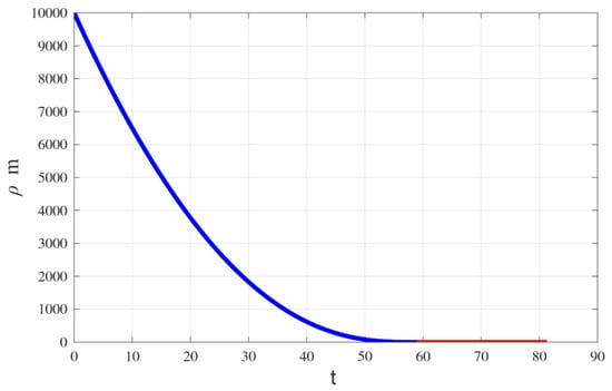
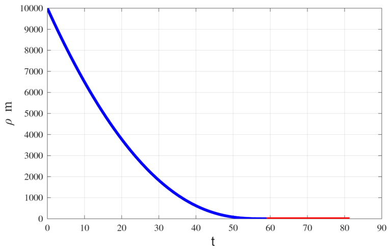
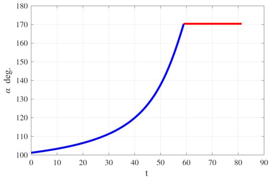
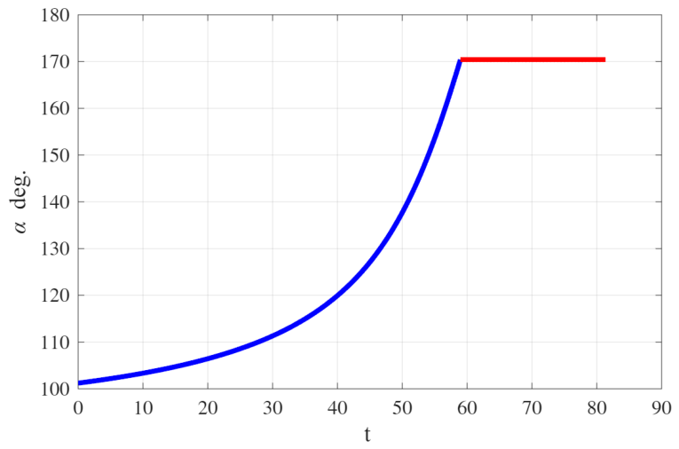
Figure 2 and Figure 3 give and the angle of the control force for a broken extremal, the second phase is red colored.
Figure 2.
, , for a broken extremal.
Figure 3.
, , for a broken extremal.
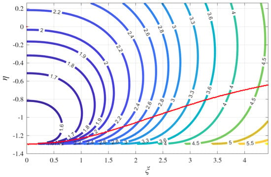
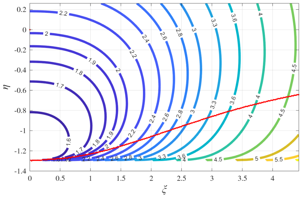
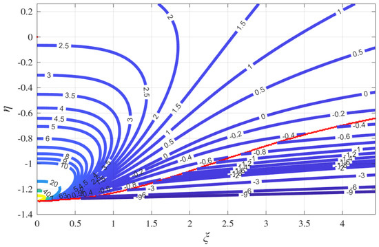
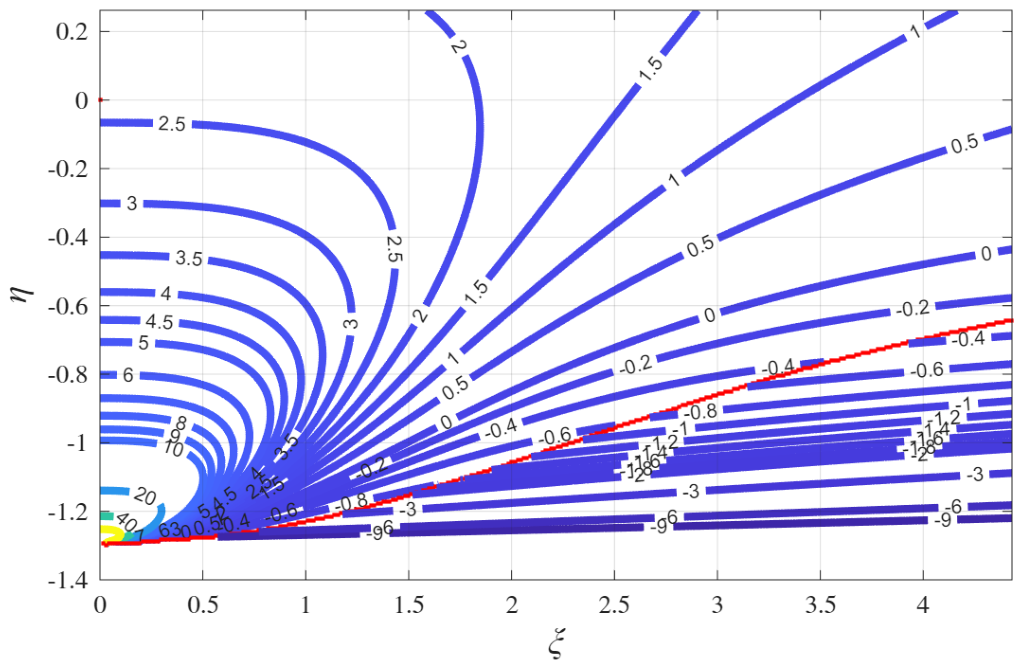
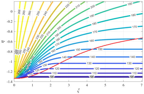
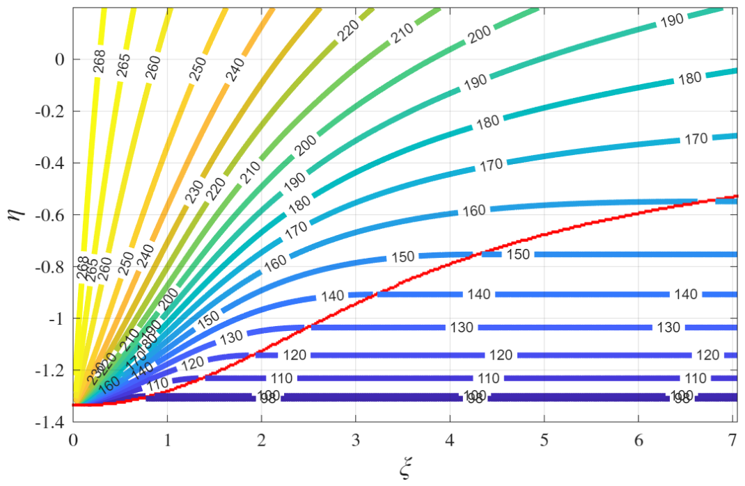
Figure 4 gives the cost in , it includes the states generating broken (below the red line) and smooth extremals studied in the next chapter. The cost is given in coordinates corresponding to , . For the problem the set , the cost and the costates-that are its derivatives- depend only on these two variables . This allows us to illustrate the optimal control mapping as a 2D transformation as will be shown in the next chapter.
Figure 4.
The function which provide the Value Function when , in the full Controllable Set. , . The red line marks the boundary between the states generating smooth extremals and those generating broken ones.
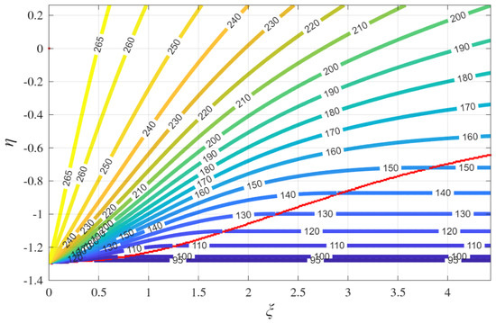
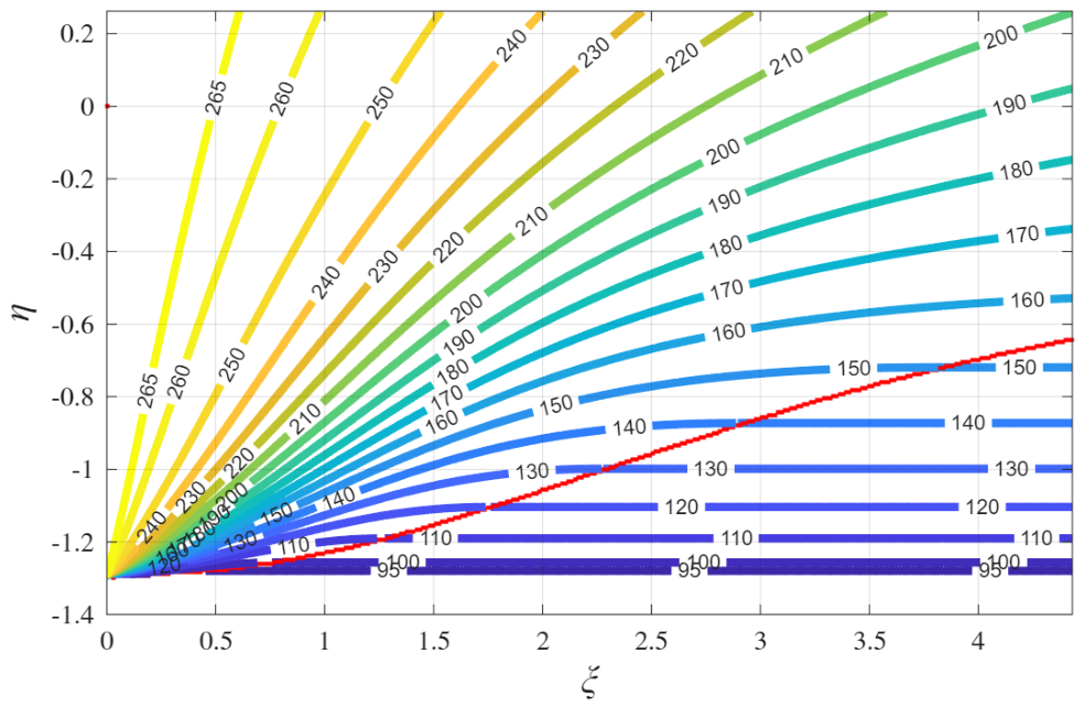
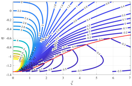
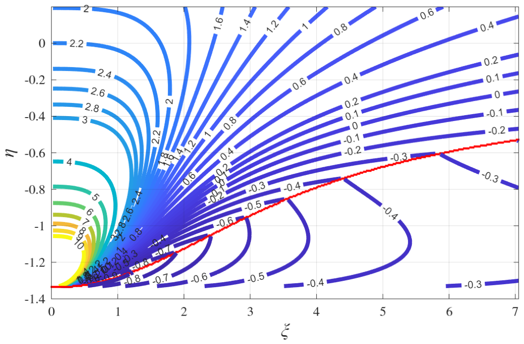
Figure 5 gives the value of . Figure 6 provides the value of . This is the 2D mapping which provides the optimal guidance. The states above the red line generate smooth extremals and those below, the broken ones.
Figure 5.
deg. with and . , . The red line marks the boundary between the states generating smooth extremals and those generating broken ones. At we have the boundary of the Controllable Set that match the value of Figure 1 at . In the region between have the states with broken extremals solutions.
Figure 6.
with and . , . The red line marks the boundary of the controllable domain for smooth extremals.
5.3. The Smooth Extremals
Smooth extremals are those which do not have a discontinuity in the costate. In order to fully characterize the smooth extremals we need to consider that at when , must be positive otherwise we would arrive to the target from underground. Thus we can use for guidance only extremals for which , which in other words can be written
Which is a necessary condition for any smooth extremal.
5.4. A Representation of the Set Covered by Smooth Extremals in Terms of Costates
In this section we are going to characterize the domain in which the costates give a smooth extremal solution. Being the case under analysis the mass is constant and we need to analyze only the constraint . Let us denote
We use as unknown instead of because the latter is not bounded and goes to infinity in the proximity of the landing point (as will be seen in Section 5.6). The conditions are written from (21)
Introducing the second equation of (31) in the third we get
Recalling that , we define
Then
in the domain . In the same domain we have also
Equations (34) and (35) can be used to solve and from . The solutions and are shown in Figure 4 and Figure 5 for . Equation (35) explain why, in the problem, we can parameterize cost and costates in terms of .
The figures show also the subset of the controllable domain that generates smooth extremals. Let us denote by the curve in red in these figures. If we compare these figures with of Figure 1 at , we find that the region between and is in the Controllable Set and admits only broken extremals which require a final horizontal braking phase.
The domain is limited by the condition and by the necessary condition (29) that in our new notation is written
From Equation (36) we derive that , introducing Equation (36) can be written , squaring which we obtain
The curves and intersects at with ( deg. for ). When 90 deg. the active constraint is:
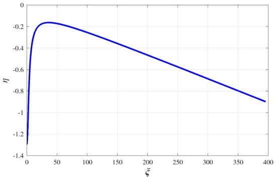
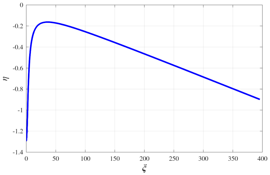
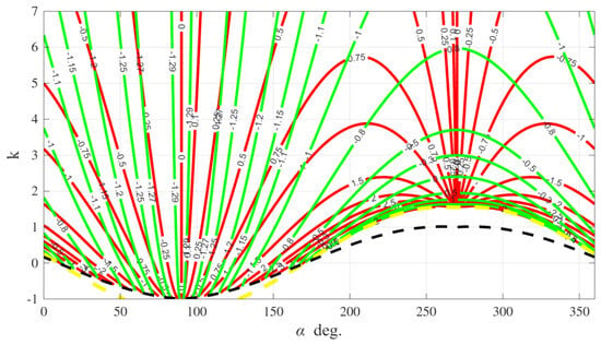
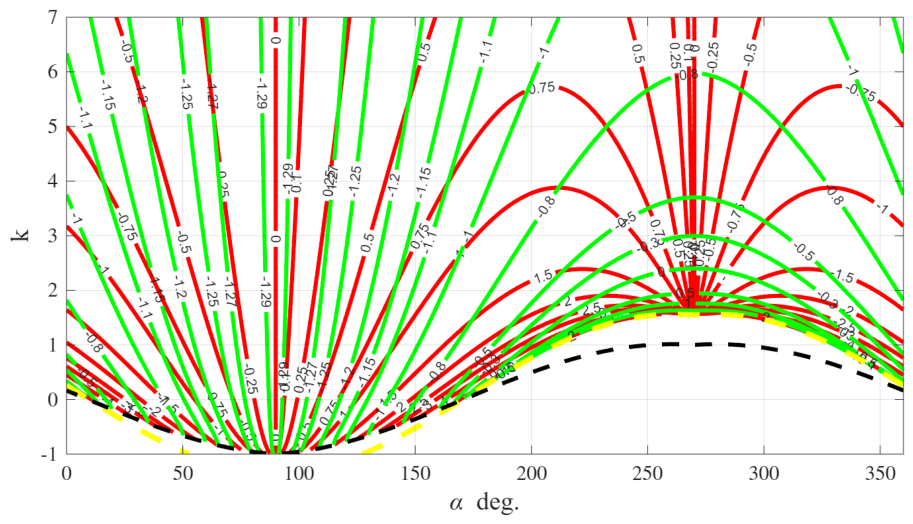
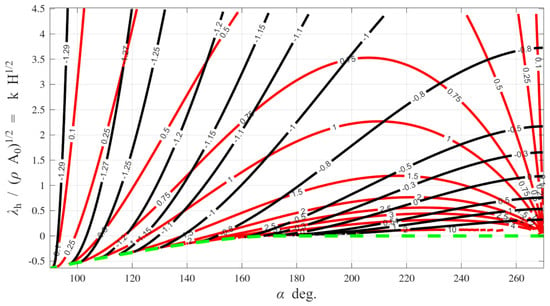
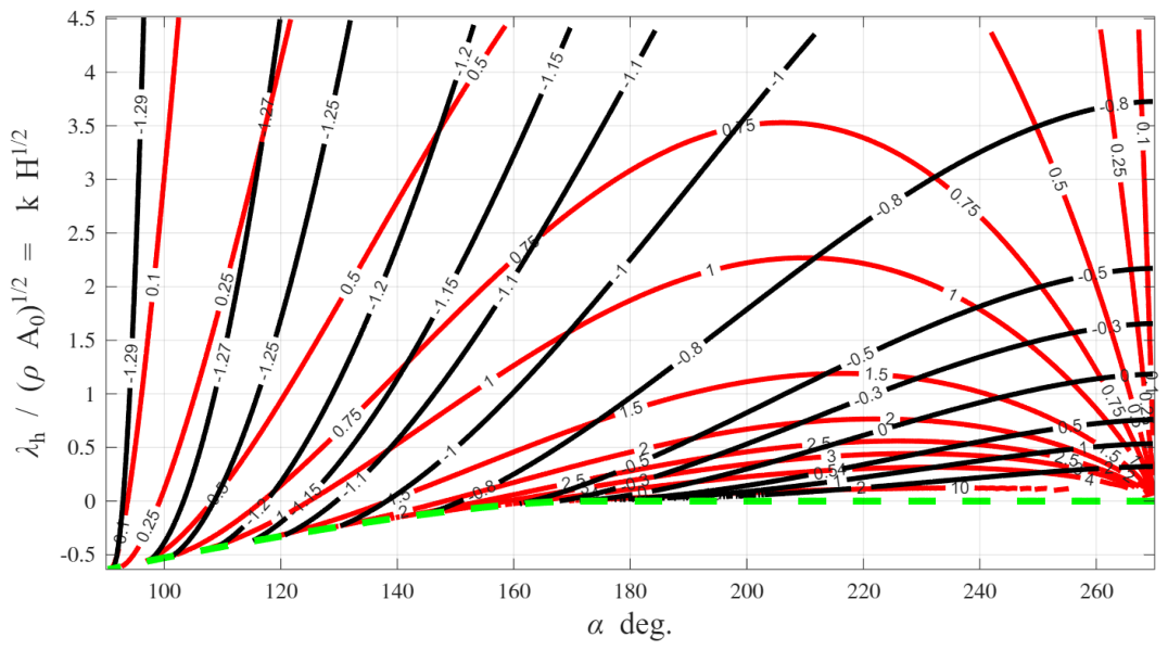
, instead when 270 deg. the active constraint is . The curve shown in Figure 7 for large values of , has a maximum at and then decreases reaching the boundary of the Controllable Set at where . Consequently the set of the broken extremals is bounded (the function grows from at to 550 at almost linearly in on ). The iso-value curves of are shown in Figure 8 in the plane. Intermittent lines show the boundaries of the Controllable domain, (yellow) and Equation (37) (black) for smooth extremals we observe that the mapping (35) is bi-jective in the domain bounded by deg. and Equation (37) to its image in the domain . Indeed the iso-value curves never cross twice therefore the mapping is one to one in this domain. This does not apply to the line deg. which for any value of k is mapped on the same point which is the only singular point of the mapping.
Figure 7.
, for large values of .
Figure 8.
iso-value (in red) (green) in coordinates, , case. Intermittent lines show the boundaries of the Controllable domain, (yellow) and Equation (37) (black) for smooth extremals.
5.5. The Vertical Fall:
The vertical fall occurs when and is obtained in our extremal solutions in the limit or . In this limit the extremal solution of Equation (33) becomes
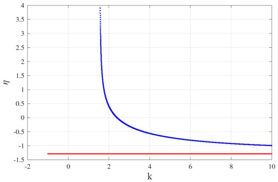
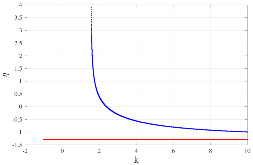
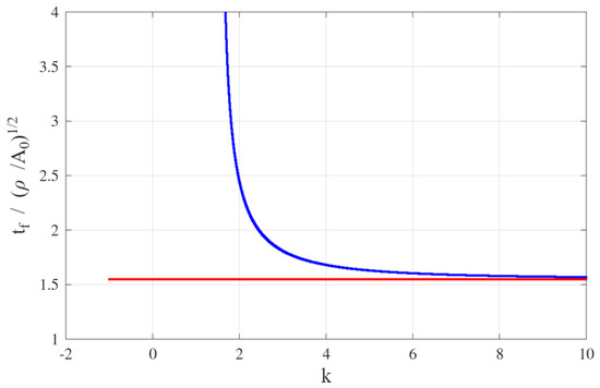
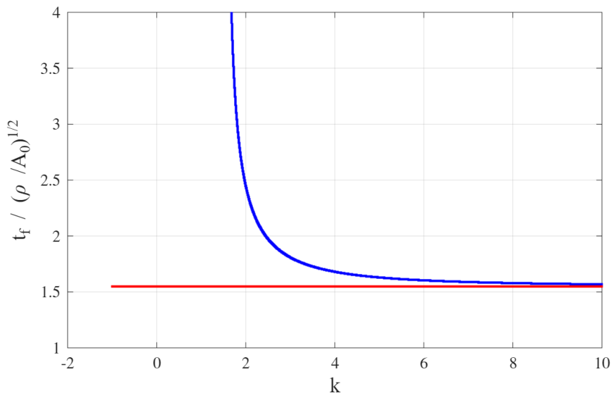
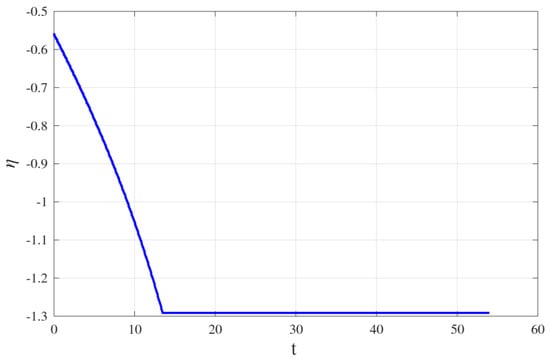
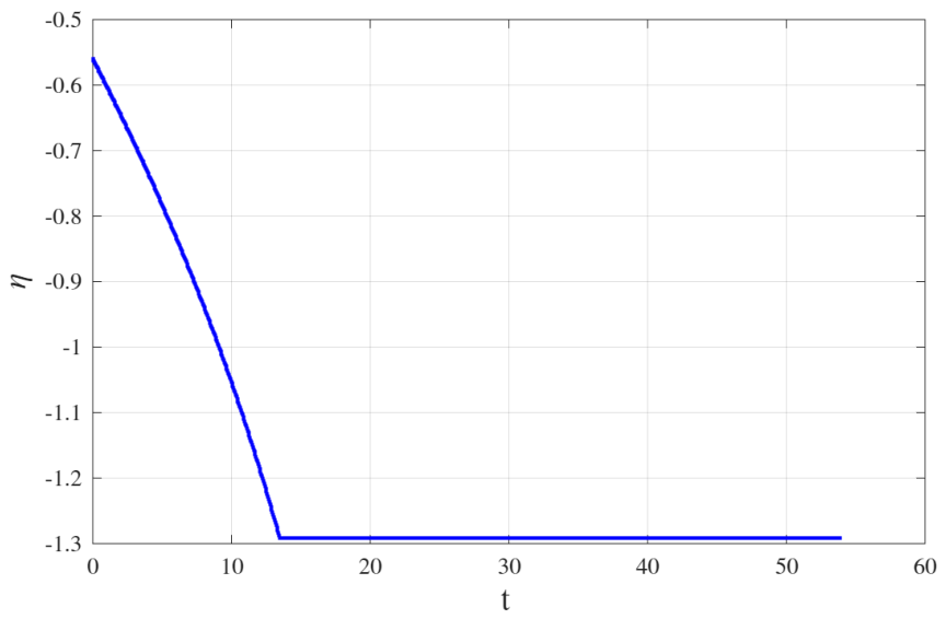
We have two possible cases and . We solve in k the first of Equation (39) and then we find with the second. The case is when we start the fall thrusting upward, the case is when we start thrusting downward and then brake later on. The solution is illustrated in Figure 9 and Figure 10 which give and the non dimensional as function of k. Figure 11 give as function of time. The red lines denote the solution with deg., and during it remains constant. The blue line denotes the solution with deg. and has a vertical asymptote at . Figure 11 give the dynamics of in an optimal vertical fall with the acceleration phase followed by the braking phase. Note that the braking phase is mapped at the single value which is the solution of Equation (10).
Figure 9.
Vertical fall: as function of k with and . The red line give the solution for deg., the blue one for deg.
Figure 10.
Vertical fall: the non-dimensional cost as function of k with and . The red line give the solution for deg., the blue one for deg.
Figure 11.
Vertical fall extremal: with the acceleration phase followed by the braking phase. and .
5.6. The Down-Scaled Value Function and Its HJB
To establish the minimality of all the extremals, we need to determine that they are the characteristics of a Value Function that is the unique solution of its Hamilton Jacobi Equation.
We note from Figure 4 that is continuous in the controllable domain . We call the down-scaled Value Function. On the contrary the Value Function is unbounded at the landing point. We can calculate the derivatives of in terms of .
where are the derivatives in the first and in the second argument. The costate is singular at and cannot be expressed only in terms of the coordinates. Introducing the gradients of inside the Hamilton Jacobi Equation (13) using the Hamiltonian (22), we obtain the following first order PDE for the down-scaled Value Function
This equation must be integrated with the boundary condition of the cost determined by (11) plus the cost of braking (28) on the hyper-surface determined by Equation (10). So at we have as boundary condition
In line with the cost given in Figure 4.
5.7. The Minimality of the Extremals
The down-scaled Value Function depicted in Figure 4 solves Equation (41) and verifies its boundary conditions. This can be easily demonstrated by numerical differentiation. If we could demonstrate that the solution of Equation (41) is unique, this would allows us to demonstrate that the extremals we have determined are the minimal cost solutions.
However we cannot use the classical theorems of uniqueness for the Dirichlet problem of HJB because Equation (41) is not a proper Hamilton Jacobi Equation for it fails to be non decreasing monotonic in for . Indeed, from ref. [19] Th.III.1 we have the following conditions to establish the unicity of the viscosity solution of a PDE in a domain with : (1) F must be uniformly continuous in all its arguments, (2) and , (3) uniformly continuous, (4) .
In order to demonstrate the minimality of the extremals we need a more complex approach with two passages.
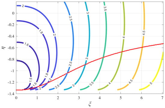
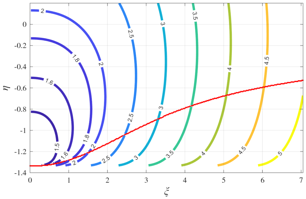
First, we asses the minimality of the smooth extremals by considering that for any given state with we have only one extremal passing through that state. This derive by noting that there is no broken extremal departing from the smooth extremal domain and looking at Figure 12 where we plot the iso-value of as function of the costate and at that state-point. We have mapped the states with the costates at a given altitude and, to do that, we had to apply a transformation to the mapping given in Figure 8 passing to the mapping . The iso-value curves never cross twice, therefore at each state where we have a smooth extremal we have only one possible costate that verifies the necessary conditions. In Theorem 2 we have proved that in we have at least a minimum solution, thus that one extremal can only be a minimal solution.
Figure 12.
iso-value (in red) (black) in coordinates, , case. Intermittent lines show the boundaries of the Controllable domain, and Equation (37) (green) for smooth extremals.
The second passage starts noting that in Section 5.4 we found that all the points of the broken extremals domain are in a closed and bounded set determined by and consequently, Equation (41) is proper (in the sense of [19] Th. 2.20) and its solution is unique if appropriate boundary conditions for a Dirichlet problem are given in the broken extremal domain (see [19] Th.III.1). These boundary conditions are given at from Equation (42) and on the curve . On this second boundary is calculated via the smooth extremals. In conclusion.
6. The General Case
To solve the problem for we need to use the integrals derived in Appendix B. In this case we are going to construct the Value Function from the extremals without demonstrating that they are unique.
The state is and the constraint on the consumable propellant must be considered. The guidance acceleration is no more constant and will be denoted by . It is convenient to use A as state variable in place of m, its dynamics is easily calculated . We will show that in a section with constant A and the topology of the smooth extremals and broken extremals domains does not change with respect to the case .
6.1. Smooth Extremals
In Appendix B we derive Equation (A12) which liase the control action to the current state in terms of three function of two arguments.
Remark 2.
In the Appendix B we have denoted the current state and costate with the subscript 0 as starting point of the extremal propagation and the final state without such subscript, from now on, we delete this subscript and denote the current state where we evaluate the control action.
The solution of system (45) in terms of for each state can be obtained numerically. In Appendix B we provide in terms of transcendental functions and is provided for positive k in power series of a with coefficients functions of . This series converge for any . For a good numerical approximation is obtained by direct numerical integration.
Equation (45) have the role of Equation (35) for the case and converge to them as . They allow us to solve for each given state the control action and the Value Function and the parameter k.
The Figure 13, Figure 14 and Figure 15 give the a section of the solution at = 15,000 m and . The red line separates the states generating smooth and broken extremal. Compare these figures with their equivalent (4), (5), (6) of the case. It is quite evident that the values of are reduced because the guidance acceleration increases in time, but the controllable domain shape as well as the control action as function of are similar to the case. Using the variables to express the the Value Function , its partial derivatives are
Figure 13.
with , at = 15,000 m, the red line is a section of marking the boundary of the states generating smooth and broken extremals. .
Figure 14.
deg. with , at = 15,000 m. .
Figure 15.
with , at = 15,000 m. .
Introducing the Value Function gradients in the Hamiltonian (6) we get
with boundary conditions resulting from the solution of system (7) at . Equation (48) gives (41) if we set and let . The properties of the two PDE are similar and (48) is proper in . We assume that a study similar to what has been done for (41) could be done also in this case.
6.2. The Broken Extremals and the Horizontal Braking
The condition here becomes (from Equation (20))
This condition with equality is used to determine the broken extremals together with .
In Figure 13, Figure 14 and Figure 15, the red line marks the boundary between the smooth extremals and the broken ones. This line is determined by having together with also so that Equation (49) is verified with the equal sign. When the extremal is divided in two intervals; the first ends at where , the second interval from to is an horizontal braking. Denoting and (from ) this second part verifies in
has a positive jump when the extremal encounter the surface , after it varies remaining continuous and we can verify that remains a function with positive variation and the necessary conditions are verified. By definition , so that .
It follows that and .
The braking duration must be found integrating the horizontal equation
This integral has a closed form primitive and the braking time can be determined with the expression
From (52) we derive that
Equation (53) can be inverted to calculate as a function of with few numerical iterations.
6.3. The Vertical Fall
The vertical fall in the case is treated in detail in [2] to which we refer. Let . Any optimal control in the Controllable Set is described by three times and , and . When the optimal landing occurs with and we are left with only two possible optimal sequences, with no coasting arcs, as in the cases treated in this paper.
7. A Closed Loop Example: Landing After a Temporary Failure
Massive Moon landers able to transport up to 100 tons payloads and a human crew are being designed for the Artemis mission, they are designed to re-enter in orbit a after the landing and to land in a single stage from the orbital conditions. We have considered in our exercise the following characteristics of the lander: Dry mass Kg, Payload mass Kg, Propellant Kg (Ox/Meth), Thrust N, m/s, m/s2 , = .
We have created a look-up table which allows us to calculate and in a grid of points in the plane. With this table we have calculated the dynamics of the landing extremal. To test the guidance law we have simulated a stressing condition.
Remark 3.
This test is not linked to any specific type of failure considering that these landers include in their design multiple hot redundancies.
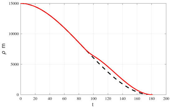
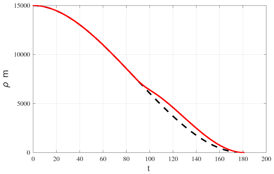
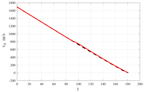
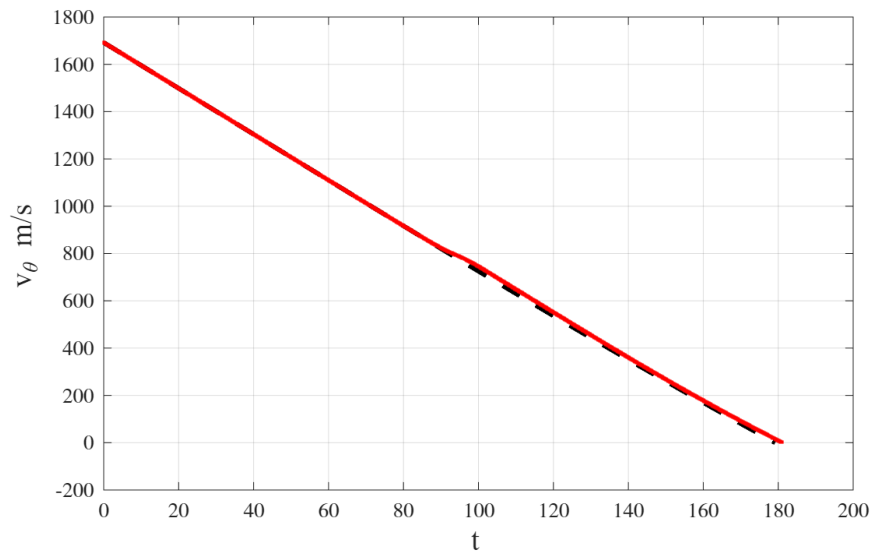
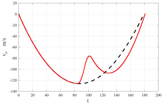
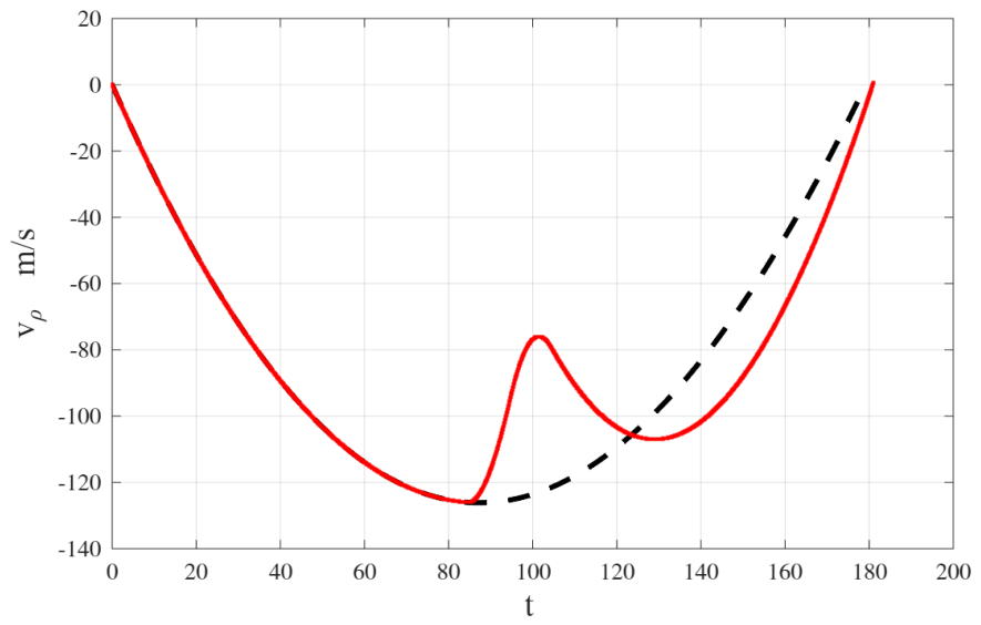
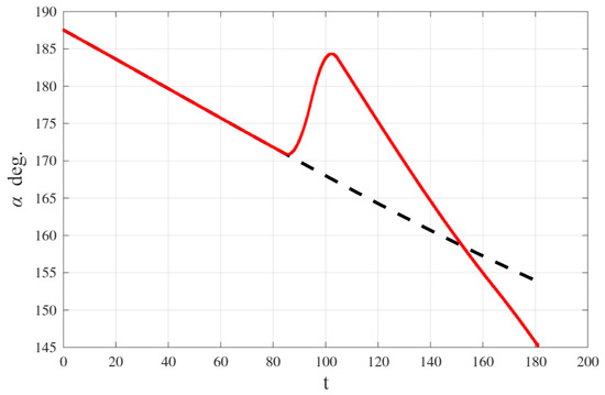
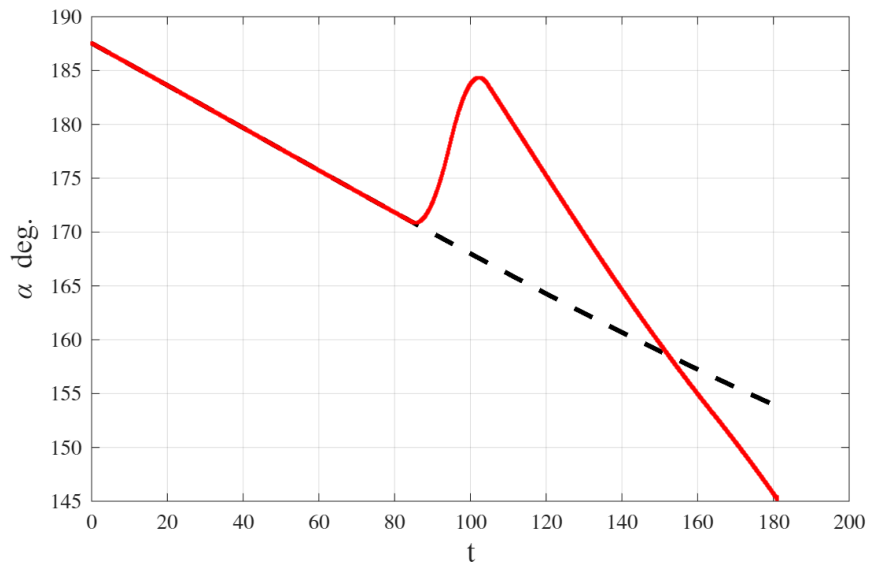
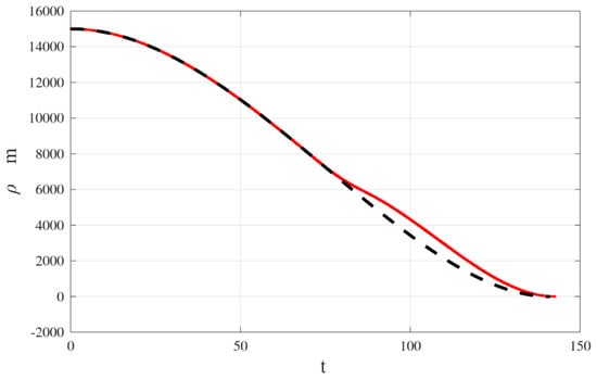
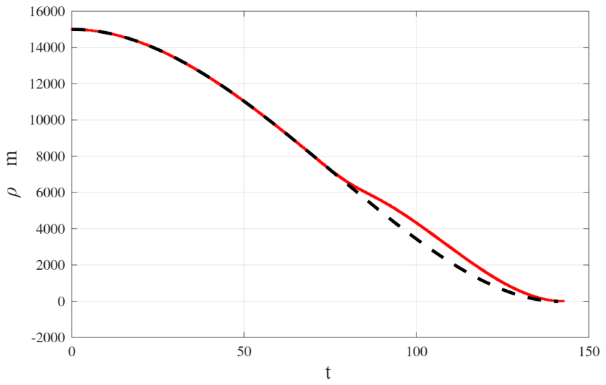
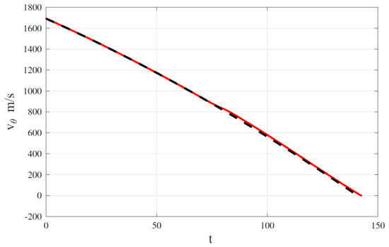
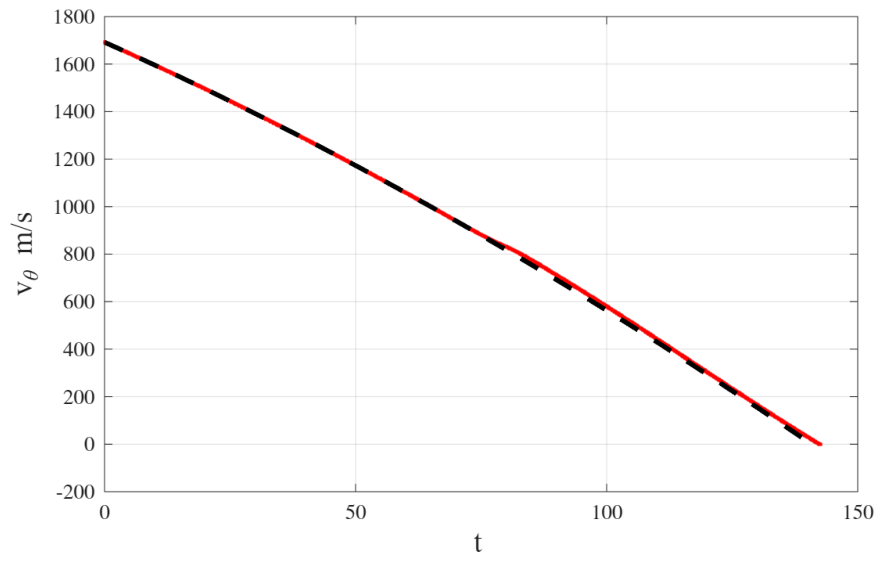
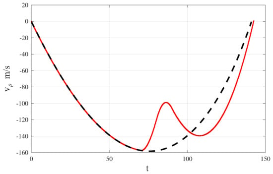
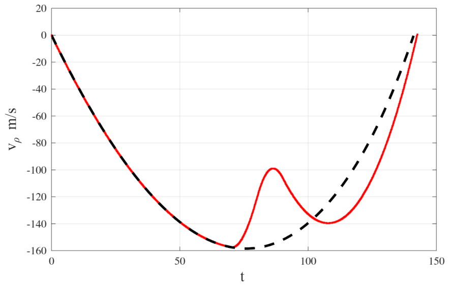
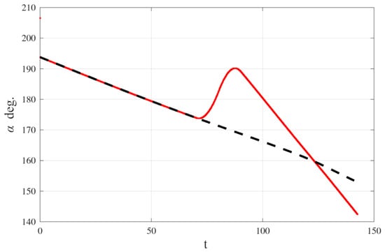
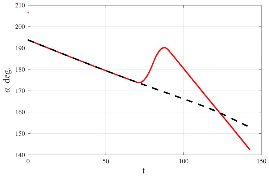
We rotated the lander and consequently the thrust direction off the optimal guidance. We added at m, a linear 45 deg. rotation to with a rise time of 10 s. After the 10 s period the correct attitude is recovered linearly in additional 10 s. The look-up table provides the optimal guidance from the state at any time. The two landing curves are shown in Figure 16, Figure 17, Figure 18 and Figure 19 for the case . In Figure 20, Figure 21, Figure 22 and Figure 23 we provide the same example calculated for . The dashed black lines provide the dynamics of the nominal extremal, the red continuous lines give the dynamics of the state and for the extremal before and after the failure. The parameters of this numerical exercise are those of a Moon landing from the initial conditions: = 15,000 m, m/s, m/s.
Figure 16.
Landing after a temporary failure: with .
Figure 17.
Landing after a temporary failure: with .
Figure 18.
Landing after a temporary failure: with .
Figure 19.
Landing after a temporary failure: with .
Figure 20.
Landing after a temporary failure: with .
Figure 21.
Landing after a temporary failure: with .
Figure 22.
Landing after a temporary failure: with .
Figure 23.
Landing after a temporary failure: with .
Thrust and mass are such that with m/s2 the nominal Moon gravitational acceleration at the surface. The nominal final time for this optimal landing is s with and s with , while the optimal guidance law after the deg. rotation give an optimal landing at s with and s with . The simulation has been repeated using a value of for the environment and the control synthesis and repeated with a value of only for the environment.
Remark 4.
The real variability of is in the order of , hence much smaller than the one applied.
The results obtained are almost identical in the two cases with different Moon gravity with an error in the final altitude less than one meter. This result indicates the robustness of the method.
Analyzing the dynamics with and without failure we note that the dynamics, results to be very different in the two cases, which brings us to think that a perturbation technique like the Neighboring Optimal Guidance would fail to recover.
8. Discussion
In this paper we have studied the structure of the optimal policy of the landing problem in the Controllable Set. The policy structure is similar in the case and . We have shown that it is possible to guide the lander using a mapping of the optimal control versus the state. We think that this full mapping approach is safer than any on-line indirect or direct method for landing. The drawback of this method is that it requires to load on board the full optimal map. How to represent it considering non flat planet, 3D descent and variable gravity is a challenge that probably will require some form of data compression. This will be subject of further studies which may involve Machine Learning techniques.
Funding
This research received no external funding.
Data Availability Statement
All datasets presented in this article are not readily available because the data are part of an ongoing study. Requests to access the datasets should be directed to author. The original data presented in the β = 0 case of the study are openly available at https://github.com/lmazzini1960/Moon-Landing-Control (30 June 2026).
Acknowledgments
I thank Piermarco Cannarsa for the enlightening discussions we had on the HJB conditions of unicity.
Conflicts of Interest
Author Leonardo Mazzini was employed by the company Thales Alenia Space. The remaining authors declare that the research was conducted in the absence of any commercial or financial relationships that could be construed as a potential conflict of interest.
Abbreviations
The following abbreviations are used in this manuscript:
| HJB | Hamilton Jacobi Equation |
| TBVP | Two Boundary Value Problem |
| ODE | Ordinary Differential Equation |
| PDE | Partial Differential Equation |
Appendix A. The Planet Surface Curvature and Central Gravitational Field
We consider the case of the Moon. The Moon has a radius of about 1738 km. Considering a landing from an altitude of 15 km with an initial orbital speed of 1692 m/s, using the parameters considered in this paper the landing occurs about 250 km in the horizontal forward direction from maneuver start. An open loop guidance will give a landing error in the ρ direction of about 20 km due to the curvature of the planet. With a closed loop guidanc, the error will be negligible in reaching the target but the trajectory will not be optimal. Defining with the orbital anomaly, the dynamic constraints to be used considering the curvature are simply the orbital equation in polar coordinates:
where is the gravitational acceleration at and R is the planet radius (see [20], Eq. 7.1 written in polar coordinates). We can derive easily the Hamiltonian and the controls for this general model:
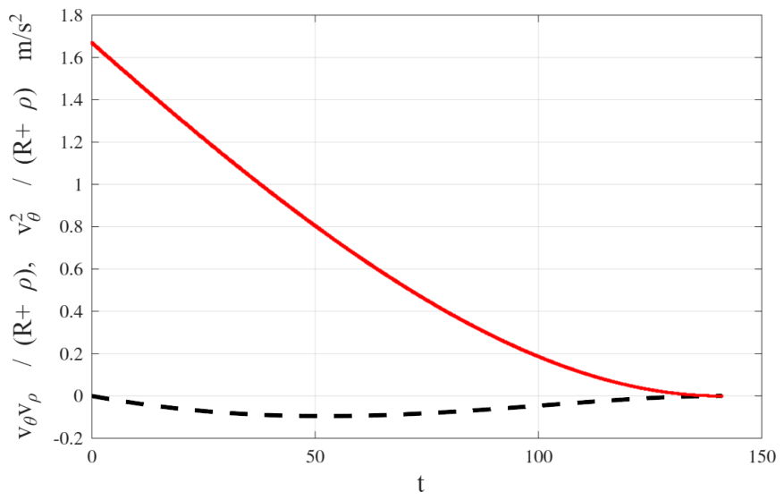
Some considerations can be formulated without deep analysis. It is easy to see that Theorem 1 applies also in this case as well as the characterization of the Controllable Set given in Theorem 4. The extension of Theorem 2, to this model is not immediate because of the non-linear dynamics, however due to the linearity of the dynamics with respect to the controls and the convexity of the control set we assume that with some effort a similar results could be obtained. The classification of broken and smooth extremals shall apply also in this case because it is due to the presence of the state constraints. Thus the solution should have similar characteristics to what we have studied in this paper and this can be proved only by further studies. For the simulation case studied, the non linear terms are quite small with respect to the control force, therefore another possible implementation of the guidance could consists in balancing them with the control. Figure A2 give these non linear terms from the example with nominal feedback and .
Figure A1.
Landing after a temporary failure: with .
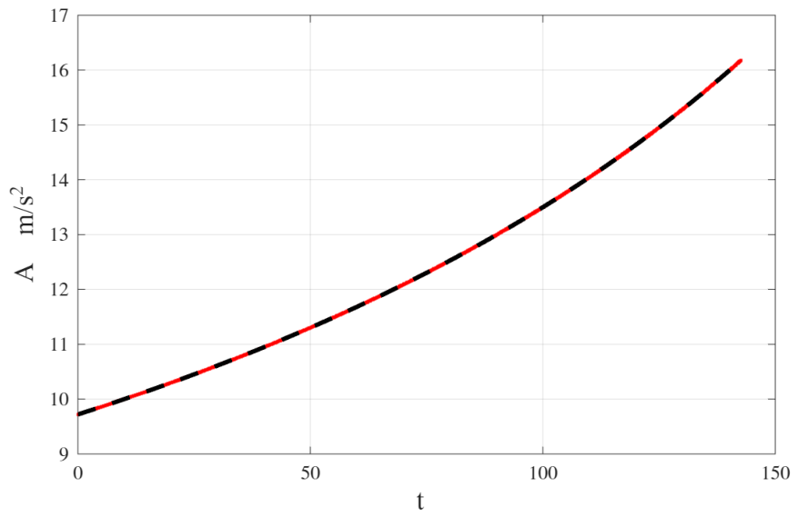
Figure A2.
Landing after a temporary failure: non-linear accelerations in dashed black and in red, with .
Appendix B. Integrals of the Extremals for β > 0
In this Appendix we integrate the extremals ODE:
Integrating we get:
We integrate Equation (A6) using the substitution method by introducing a new integration variable
w has a positive derivative with respect to time if and negative when . Thus we have to reverse the integration limits depending on the sign of h.
We need to express in terms of w.
with the position
Considering that the integration limits are when and when and that , the integrals of and , for any value of h, are transformed in:
These integrals are defined provided that which is always true in because , putting aside the case when the integral boundaries coincide. Let us introduce the following primitives:
using which we determine the solution of our problem ():
Introducing the final conditions we have the following set of equations to determine the costates and :
From the last equation we get:
Thus the problem is fully solved finding the primitives Equation (A10). First we assume , the primitives can be easily found:
When we consider only the first two primitives can be expressed in closed form:
Note that . cannot be expressed in closed form, however it can be developed in series of a or of k, the series of a is derived by developing and then integrating each term of the series:
It is possible to verify the convergence of this series in .
Appendix C. Proof of Theorem 1
Theorem A1.
Each state in the controllable set admits an optimal control , for some finite , which gives the minimum of the functional (1), verifies the constraints in and reach at .
Proof.
Take any point in . From the hypotheses there is an admissible control which drives the state from the initial state to in a finite time and with a final mass such that in . Consider the set of all the controls , that satisfying the constraint and , drive the state in at some and after are continued with in . We prove that any sequence of controls in converging in the norm converges inside . Indeed take a sequence converging in . Using Gronwall Lemma and denoting by the first three components of the state and by we have the estimate , from and Gronwall Lemma.
Consequently converge in which is complete in the norm . Hence the constraints hold true in the limit of the sequence. Concerning the fourth state , but for the Jensen inequality. The norm is continuous in the metric therefore also the constraint holds true in the limit of the sequence. Thus is closed and bounded in a ball of of norm , therefore it is weakly sequentially compact in (see [18] Theorem 5.40: any closed, bounded and convex subset of a Reflexive Banach Space is weakly compact. In addition a closed subset of a compact space is compact.). Consider a minimizing sequence so that . Let the corresponding state sequence and the first time in which . Being monotonic decreasing and bounded below, . Similarly, being weakly sequentially compact, we can extract a minimizing sub-sequence converging to some and . Hence is the control that realizes the minimum cost. The state trajectory corresponding to is . □
Appendix D. Proof of Theorem 3
Theorem A2.
Let be the hyperplane of points with mass m. The set is convex. if .
Proof.
Consider two points in with the same initial mass . Each of the two has a minimal trajectory and and a minimal final time and . Assume . Hence . Let us prolong the first trajectory up to the time by keeping in , . This is feasible because is an equilibrium point and we have spare mass in the first solution. Now the two trajectories end at the same time and have the same mass at any time in . Due to the convexity of the control set and the linearity of the system first three equations we deduce that any solution will be at the target at time . □
References
- Bellman, R. Dynamic Programming; Princeton University Press: Princeton, NJ, USA, 1957. [Google Scholar]
- Gazzola, F.; Marchini, E.M. A Minimal Time Optimal Control for a Drone Landing Problem. Esaim Control. Optim. Calc. Var. 2021, 27, 99. [Google Scholar] [CrossRef] [Scilit]
- Vinter, R. Optimal Control; Modern Birkhauser Classics; Birkhäuser: Boston, MA, USA, 2000. [Google Scholar]
- Cannarsa, P.; Sinestrari, C. Semiconcave Functions, Hamilton Jacobi Equations, and Optimal Control; Birkhauser: Basel, Switzerland, 2004. [Google Scholar]
- Intelisano, A. New Trends and Challenges in Optimization Theory Applied to Space Engineering, Artificial Intelligence Algorithms for Space Missions; Optimization and its Applications; Springer: Cham, Switzerland, 2023; 221p. [Google Scholar]
- Ghosh, P.; Woodburny, J.; Short, C. Approximate-Optimal Feedback Guidance for Soft Lunar Landing Using Gaussian Process Regression; American Astronautical Society (AAS) 17-790; American Astronautical Society: Springfield, VA, USA, 2017. [Google Scholar]
- Acikmese, B.; Ploen, S.R. Convex Programming Approach to Powered Descent Guidance for Mars Landing. J. Guid. Control Dyn. 2007, 30, 1353–1366. [Google Scholar] [CrossRef] [Scilit]
- Pontani, M.; Cecchetti, G.; Teofilatto, P. Variable-time-domain neigh- boring optimal guidance, part 1: Algorithm structure. J. Optim. Theory Appl. 2014, 166, 76–92. [Google Scholar] [CrossRef] [Scilit]
- Hull, D.G. Optimal Guidance for Quasi-Planar Lunar Descent with Throttling. In Proceedings of the 21st AAS/AIAA Spaceflight Mechanics Meeting, New Orleans, LA, USA, 13–17 February 2011; pp. 983–994. [Google Scholar]
- Martinez, R.C.; Kumar, K.D.; Cortez, H.R. Precise power descent control of a lunar lander using a single thruster. Acta Astronaut. 2021, 186, 473–485. [Google Scholar] [CrossRef] [Scilit]
- Capolupo, F.; Rinalducci, A. Descent and Landing Trajectory and Guidance Algorithms with Divert Capabilities for Moon Landing. arXiv 2023, arXiv:2305.13846v3. [Google Scholar]
- Pontani, M.; Celani, F.; Carletta, S. Lunar descent and landing via two-phase explicit guidance and pulse-modulated reduced-attitude control. J. Optim. Theory Appl. 2014, 212, 672–685. [Google Scholar]
- Pontani, M.; Cecchetti, G.; Teofilatto, P. Variable-time-domain neigh- boring optimal guidance, part 2: Application to lunar descent and soft landing. J. Optim. Theory Appl. 2014, 166, 93–114. [Google Scholar] [CrossRef] [Scilit]
- Lu, P. Propellant-Optimal Powered Descent Guidance. J. Guid. Control. Dyn. 2018, 41, 813–826. [Google Scholar] [CrossRef] [Scilit]
- Gazzola, F.; Marchini, E.M. New Trends and Challenges in Optimization Theory Applied to Space Engineering, Optimal Control for the Moon Lander: The Classical Problem and Variants; Optimization and its Applications; Springer: Cham, Switzerland, 2023; 221p. [Google Scholar]
- Frankowska, H. Optimal Control under State Constraints. In Proceedings of the International Congress of Mathematicians, Hyderabad, India, 19–27 August 2010. [Google Scholar]
- Mazzini, L. Extended sufficient conditions for strong minimality in the Bolza problem: Applications to space trajectory optimization. J. Optim. Theory Appl. 2024, 191, 486–516. [Google Scholar]
- Clarke, F.H. Functional Analysis Calculus of Variation and Optimal Control; Springer: London, UK, 2013. [Google Scholar]
- Crandall, L.G.; Lions, P.L. Viscosity Solution of The Hamilton Jacobi Equation; Transactions of the American Methematical Society: Providence, RI, USA, 1983; Volume 277, Number 1. [Google Scholar]
- Mazzini, L. Flexible Spacecraft Dynamics, Control and Guidance; Springer: Cham, Switzerland, 2016. [Google Scholar]
Disclaimer/Publisher’s Note: The statements, opinions and data contained in all publications are solely those of the individual author(s) and contributor(s) and not of MDPI and/or the editor(s). MDPI and/or the editor(s) disclaim responsibility for any injury to people or property resulting from any ideas, methods, instructions or products referred to in the content. |
© 2026 by the author. Licensee MDPI, Basel, Switzerland. This article is an open access article distributed under the terms and conditions of the Creative Commons Attribution (CC BY) license.