


Abstract
High-precision onboard orbit propagation, often unavailable due to high demands of onboard resources, is crucial for autonomous optical link pointing and acquisition in large-scale low Earth orbit satellite constellations. For such large-scale constellations, an advantageous feature for efficient and accurate orbit propagation is the correlation or similarity in the orbit perturbations experienced by multiple satellites. Yet, this correlation has not been fully utilized in existing orbit propagation methods. In this work, we propose a cross-referential orbit propagation framework that leverages multiple historical reference arcs from other satellites within the same constellation to improve prediction accuracy and reliability. The framework achieves error reduction comparable to that of ensemble learning by aggregating the predictions from a single lightweight model under varying reference inputs, thereby preserving a simple and compact model architecture. To ensure the generalizability of this compact model, we further introduce a network architecture termed the Compressive Decoder for Orbit Propagation (CDOP). The CDOP predicts low-dimensional representations of the propagated orbits, from which the full time series are subsequently decoded. By incorporating modules from pre-trained compressive autoencoders, the CDOP mitigates overfitting while maintaining a low inference cost. The proposed method is validated on simulated Walker constellations with different geometries. The results demonstrate an average 24 h position error of approximately 200 m, with an inference cost 30 times lower than that of a reduced-dynamic numerical propagator. The framework is computationally lightweight, generalizes well across different initial conditions, and is well suited for onboard deployment in autonomous optical link acquisition.
1. Introduction
In recent years, large-scale low Earth orbit (LEO) satellite constellations have been developed rapidly. To date, more than ten thousand Starlink satellites have been launched and deployed. Chinese initiatives, including the G60 and GW constellations, are also entering the race to build constellations comprising over ten thousand satellites. Driven by the sheer scale and complexity of these systems, the autonomous operation of LEO mega constellations has become an urgent requirement. The onboard capability for accurate orbit propagation is a key enabler of autonomous constellation operation and serves as the foundation for the dynamic planning and acquisition of optical inter-satellite links. For onboard autonomous optical link management with dynamic adjustability, satellites must frequently propagate their own orbits and those of other satellites using relatively limited computational resources, while the accuracy of orbit propagation critically affects the efficiency of the link acquisition process. A study [1] on the impact of pointing error on link acquisition time shows that the average acquisition time for optical inter-satellite links scales quadratically with the orbit propagation error. Specifically, when the initial pointing error is reduced from kilometers to hundreds of meters, the expected single-link acquisition time can decrease from 8 min to 48 s.
Due to intensive computational requirements, most LEO constellations adopt a ground-based framework for optical link planning and acquisition, where the ground facilities provide virtually unrestricted computational resources. Under this framework, a centralized system calculates the link acquisition windows and schedules mission plans in advance. These commands are subsequently uploaded to satellites for execution via a telemetry, tracking and command (TT & C) link at appropriate times. As a result, not only does the burden on the ground TT & C resources increase with the growth of a constellation, but the link topology is also unable to adjust dynamically in response to satellite status and traffic demands.
To enable the autonomous and dynamic management of optical inter-satellite links, this work aims to develop a resource-efficient, on-board deployable orbit propagation method. Traditionally, orbit propagation (OP) methods fall into two categories: analytical propagators and numerical integrators. The former offers low computational cost but suffers from limited precision due to its consideration of only simplified perturbation terms; the latter achieves high precision but imposes a greater computational burden. With the advancement of machine learning and increased readiness for onboard deployment of machine learning models [2,3,4], data-driven and hybrid orbit propagation methods have garnered widespread attention for their potential to achieve both high precision and computational efficiency.
Classical fitting and machine learning methods, such as Poisson series fitting and support vector machines, have been adopted to refine the accuracy of orbit propagation for more than a decade. Early researchers [5,6,7,8] proposed two-step analytical–statistical hybrid extrapolation methods, which employed traditional data fitting techniques to compensate for errors generated by analytical orbit extrapolation, effectively reducing extrapolation errors. Subsequently, Peng et al. conducted a series of studies on similar problems using various machine learning methods. Employing support vector machines (SVMs) [9,10,11], Gaussian processes [12] and one-hidden-layer artificial neural networks (ANNs) [13], they trained models on historical orbit data prior to the start of extrapolation to predict and correct errors in analytical orbit extrapolation. They also presented detailed comparative analyses of the results obtained by these methods [14,15].
Recently, deep learning based on artificial neural networks has evolved rapidly, showing impressive capability, and has been widely applied to spacecraft guidance and control [16,17,18]. Particularly for orbit propagation, following the same principle of combining analytical estimations with data-driven corrections, Li et al. [19] considered a scenario in which orbit measurement data are acquired from a single ground station. They adopted a boosting tree algorithm to learn and correct the analytical orbit extrapolation errors of three LEO satellites. The correction achieved a reduction of over 50% in the original errors, outperforming the SVM method. The same group later [20] utilized two models—a gradient boosting decision tree (GBDT) and a fully connected network—to learn and correct the orbit extrapolation errors of five LEO and medium Earth orbit (MEO) satellites, achieving an error reduction of over 75% for 14-day predictions. Curzi et al. [21] employed a long short-term memory (LSTM) network to correct the orbit extrapolation errors of four LEO satellites, reducing the SGP4 extrapolation error by an average of 45%. Zhang et al. [22] also applied an LSTM network to learn and predict the orbit data of the Ajisai satellite, with the corrected prediction accuracy reaching the order of 500 m per day. Huang et al. [23] combined XGBoost with an extended Kalman filter and trained separate models for different orbits to improve the orbit prediction error, achieving a 7-day position error of a few tens of kilometers and a 1-day error on the kilometer level. Li et al. [24] constructed a neural network model integrating an attention mechanism, CNN, BiLSTM, and XGBoost to learn and predict the orbit data of two satellites, Saral and TerraSAR-X. The prediction accuracy of this model was significantly improved compared with that of simpler models, such as LSTM and GRU.
The previous works mentioned above demonstrate the advantage of data-driven hybrid methods for improving OP accuracy while maintaining relatively low computational costs. In particular, ensemble learning methods, such as boosting trees, show significant performance improvements by aggregating predictions from diverse models, benefiting from the “wisdom of the crowd.” While a single model might produce a large error or get stuck in a bad local minimum, a group of models is statistically more likely to converge on the correct prediction and cancel out individual noise. However, the downside of ensemble learning shares the same origin: multiple models are more complex and require more memory. Although improving accuracy is the primary goal for developing our onboard orbit propagation model, the complexity and memory requirements of the model must also be taken into consideration in engineering practice.
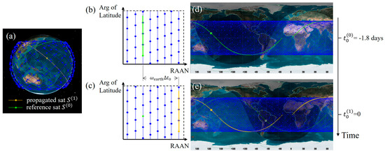
In this work, to fully leverage the reliability and performance enhancements of ensemble learning while keeping the model structure simple, we propose a cross-referential OP framework. In this framework, to propagate the orbit of one satellite in a constellation, ephemerides of several other satellites in the same constellation are taken as direct references (Figure 1). Unlike the approach in ref. [20], which trains the model on historical ephemerides and then applies the learned knowledge to other satellites, our framework explicitly incorporates several historical arcs from across the constellation as reference inputs. These references yield multiple independent estimates of the future orbit; the resulting residual errors are subsequently corrected by a neural network, following standard practice in the field. Compared to the common practice in which neural network models base corrections on a single estimation (usually SGP4 generated), our cross-referential workflow offers the capability of enhancing reliability and improving accuracy by incorporating multiple reference arcs. Instead of aggregating predictions from different models, the proposed framework aggregates predictions from the same model with different auxiliary inputs, thereby reducing the overall complexity while achieving a similar reduction in error variance. To ensure the generalizability of a single model with moderate complexity within the cross-referential framework, we propose a compressive decoder architecture. Rather than providing predictions one step at a time as in traditional sliding window frameworks, the proposed architecture learns to map the initial states to highly compressed feature vectors and then outputs the entire time series via decoding. The compressive feature extraction of the output time series facilitates the establishment of a more generalizable mapping that is less prone to overfitting.
Figure 1.
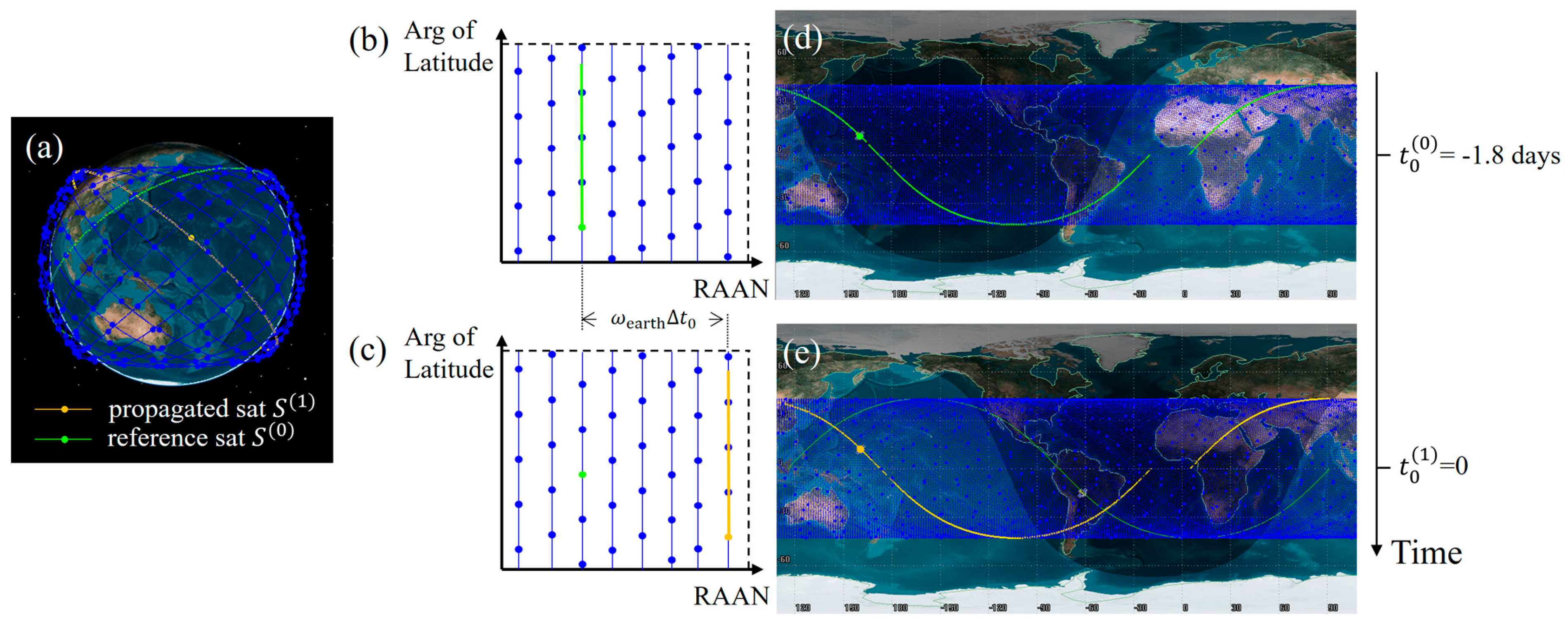
Cross-referential orbits in a Walker constellation. The yellow line represents the orbit of the satellite that needs to be propagated; the green line represents one of the orbits that serves as a reference, with a very similar ground track to the orbit that needs to be propagated. (a) The constellation viewed in an ECI frame. (b,c) Schematic plot of argument of latitude and RAAN of the reference and propagated arcs, respectively. Note that they correspond to different times and, thus, different RAANs. (d) Ground tracks 1.8 days prior to the start time of the OP. (e) Ground tracks at the start time of the OP.
2. Methods
For LEO constellations, the orbits of individual satellites are designed to satisfy specific geometric relationships. In a Walker constellation, for instance, the nominal values of the semimajor axis, eccentricity, and inclination are identical for all satellites, while the right ascension of the ascending node (RAAN) and argument of latitude are evenly spaced. Consequently, for the trajectory (specifically, the ground track) of any given satellite during any period of interest, many other satellites in the same constellation will exhibit closely matching ground tracks during adjacent time intervals. For example, within a 48 h window, more than ten satellites in a Walker constellation of 400 satellites will traverse ground tracks that lie within 2° of latitude of those of any reference satellite. These satellites experience similar higher-order gravitational perturbations as well as closely related third-body and tidal perturbations. Therefore, when propagating the orbit of a single satellite, knowledge of prior ephemerides with similar tracks can serve as valuable referential information. Such references can be particularly effective in suppressing uncertainty when predictions derived from multiple reference orbits are combined. Motivated by this observation, we developed our orbit propagation method as described below.
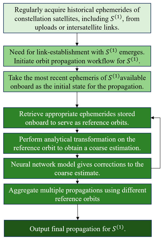
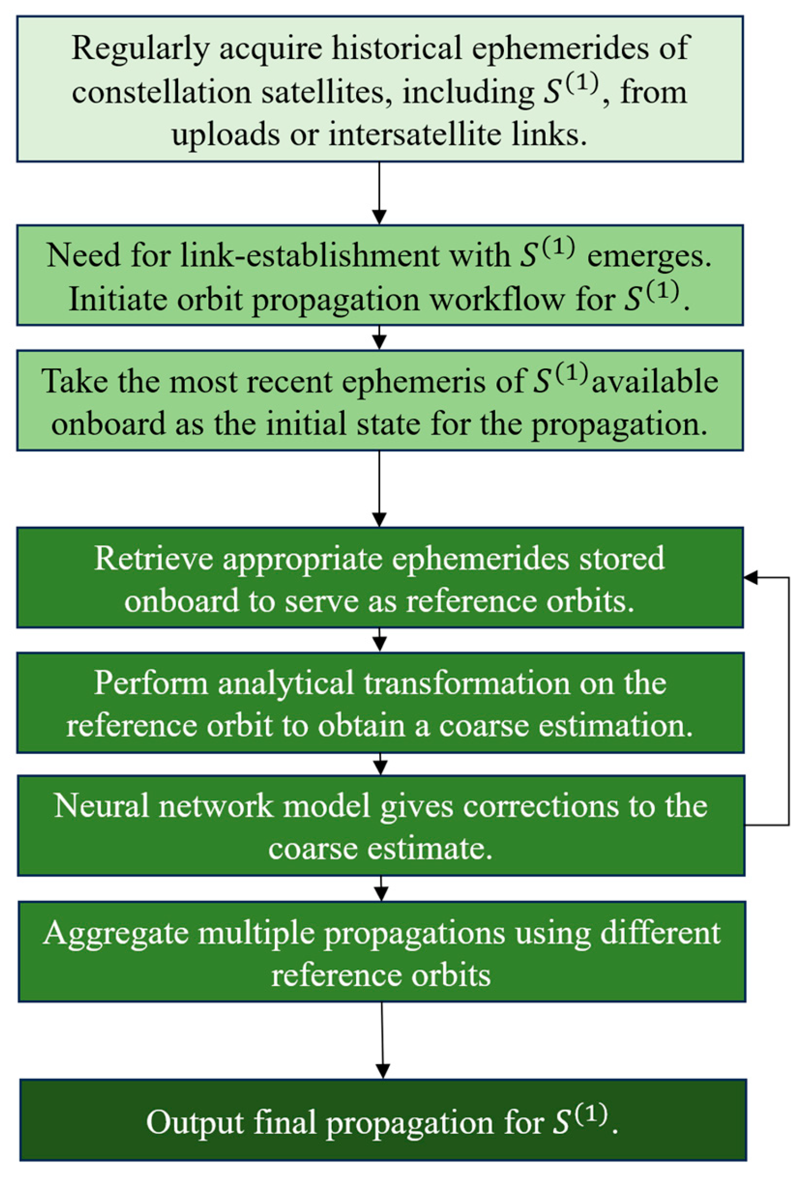
We denote the satellite of interest whose orbit is to be propagated as , the start time of the propagation as , one of the reference satellites as , and the corresponding start time of the reference arc as . For the application of autonomous optical link acquisition, short- to medium-term orbit propagation is of interest; thus, we propagate forward for 24 h. The workflow of the orbit propagation process in the context of autonomous optical link acquisition is illustrated in Figure 2. The start time of the propagation corresponds to the most recent epoch available in the onboard historical ephemerides. First, according to the longitude and the argument of latitude of at , we search the historical ephemeris for suitable such that the longitude is close to , and the arguments of latitude are the same, with the start time of the reference arc being within 24–48 h before . If is ascending, should be also ascending and vice versa. Thus, during the next 24 h starting from , the ground tracks of should be close to each other. Then, we analytically transform the reference ephemeris data of to get a coarse-grained estimation for the orbit prediction of . Next, a neural network based on a compressive decoder is introduced, taking the initial state of , with the space weather indices and auxiliary information about the reference arc used as inputs to make corrections to the coarse-grained estimation, giving one high-precision orbit prediction. Finally, multiple predictions are repeatedly given by the same previous steps but using different reference satellites , and the averaged prediction is taken as the final result of the propagation. In the following subsections we discuss, in detail, each step of our method.
Figure 2.
Flowchart of proposed cross-referential orbit propagation framework for autonomous optical link acquisition with .
2.1. Analytical Transformation for Coarse-Grained Estimation
Although a reference arc is chosen in such a way that its ground track is close to the ground track of the to-be-propagated arc, in inertial frames the two arcs are very different since they correspond to different time periods (See Figure 1a). Thus, it is not yet clear how the reference arc can give rise to a useful estimation for the orbit propagation problem of interest. In this subsection we introduce the transformation that converts the orbital elements of into a coarse-grained estimation of the predicted orbit elements of .
First, the osculating elements of at every time step, , and the osculating elements of at the initial time are converted to a simplified L. The Liu-type mean elements use the following definition [25]:
where we have omitted the superscript , standing for “reference arc”, for clarity. represents one of the six non-singular osculating elements, , and is the corresponding mean element. and are defined by
As per convention, represents semimajor axis; represents eccentricity; represents inclination; represents RAAN; represents argument of perigee; represents mean anomaly. For near-circular orbits in LEO constellations, short-period correction terms to mean elements are given by
In Equation (1) and Equations (5)–(10) above, the conversion from mean elements to osculating elements is explicitly defined. Note that the conversion is local in time in this definition; i.e., the osculating elements at time can be obtained using only the knowledge of the “mean” elements at time and vice versa. Reversely, to efficiently convert the osculating elements back into mean elements, it suffices to iteratively substitute the osculating elements into the right-hand side of Equations (5)–(10) twice. This gives with a position error within a few meters for LEO orbits, which is well tolerable for our goal regarding propagation accuracy.
We denote the mean elements of obtained by converting the historical ephemeris as with the subscript “a” standing for “actual”. Next, starting from the mean elements at and , and are propagated analytically considering only the J2 perturbations for , respectively, giving and . The J2 propagator we use is from [25].
and , . Here, and is the geocentric gravitational constant. Using the actual historical mean elements of the reference arc and the J2-propagated mean elements and , we construct the estimated mean elements for at each time step as
for. The angular wrapping in this work is handled by taking rem(, ) every time an angular orbit element is updated by addition or subtraction. The coarse-grained estimation is obtained essentially by first extracting from the reference arc the differences between the actual historical mean elements, which contain the effects of all perturbations, and the J2-propagated mean elements. These element-wise differences are then added to the J2-propagated mean elements of the satellite of interest. Performing the correction in the mean-element domain avoids explicit rotation and ensures smoothness. For example, to inherit the change in RAAN due to the higher-order non-spherical Earth gravity, the mean RAAN differences between the actual and J2-propagated orbits of the reference satellite can be simply added to the J2-propagated mean RAAN of the satellite of interest. If, instead, this is done in terms of state vectors , explicit rotations of the differences will be involved since the initial RAAN of the reference and the to-be-propagated arcs are very different (c.f. Figure 1).
Subsequently, the estimated mean elements are further transformed into state vectors in earth-centered inertial (ECI) coordinates. This is done by first converting into osculating elements using Equations (5)–(10), and then into state vectors using standard transformations.
2.2. Neural Network Model for Error Correction
Data-driven OP models are advantageous due to both their precision and computational workload, while analytical and numerical models have to make trade-offs between the two. However, their limited generalizability may hinder the application of data-driven OP methods in realistic scenarios. Technically, models based on traditional sliding window frameworks, which learn to predict only one time step based on the entire historical curves of every inference call, learn the statistics better than the orbital dynamics. A model with full orbital dynamics should be able to propagate future steps based on the initial condition involving only the start time. Therefore, traditional sliding window-based models, without amplifying errors [14], are typically less generalizable compared to models that capture the dynamics. We aim to develop a model that is capable of making accurate predictions for various initial states within a constellation without re-training, and that works consistently over an extended start time of propagation. To this end, we propose an innovative architecture based on the decoder modules of pre-trained compressive autoencoders for the orbital data, hence termed Compressive Decoder for Orbit Propagation (CDOP).
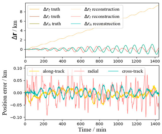
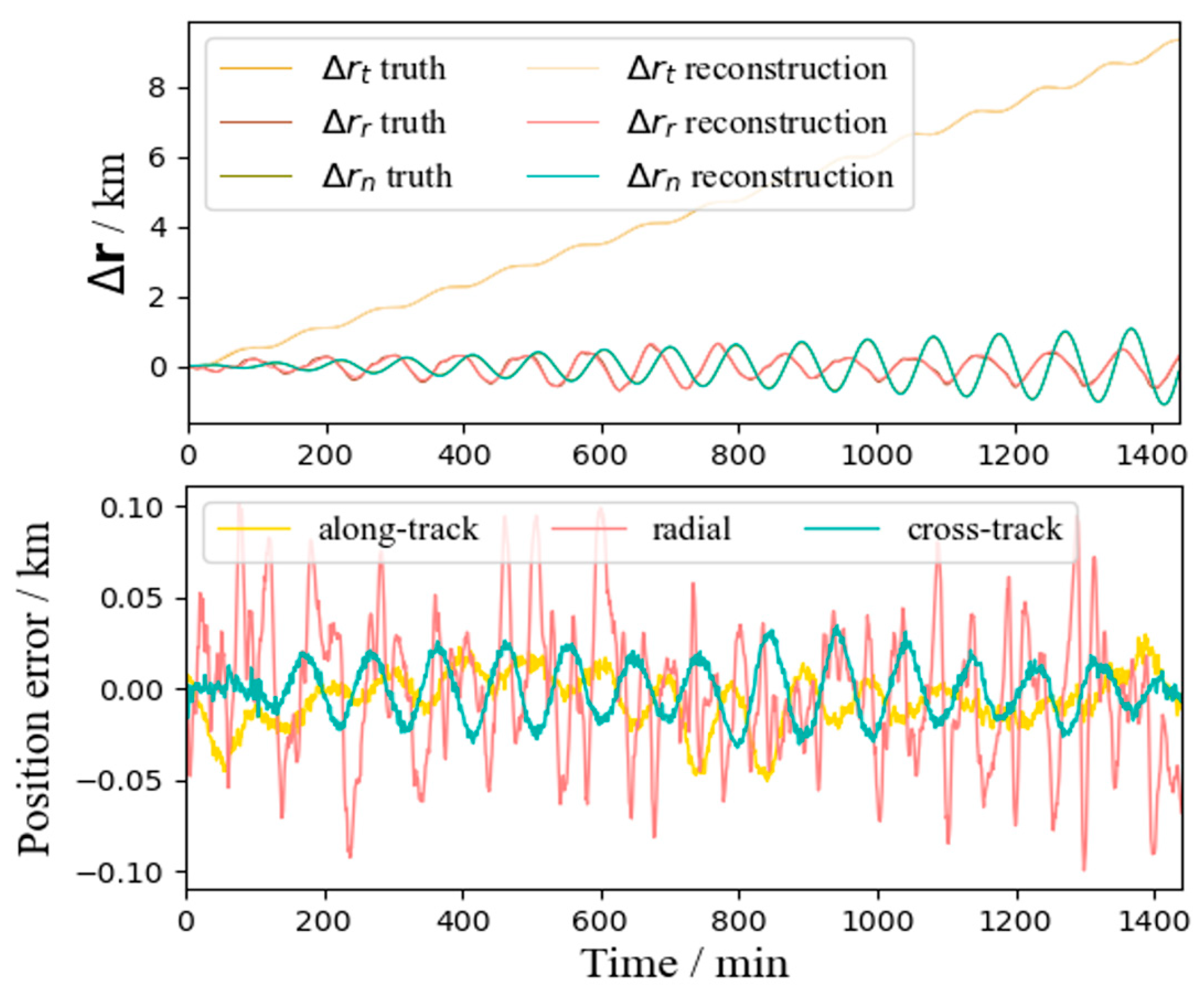
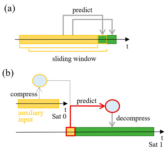
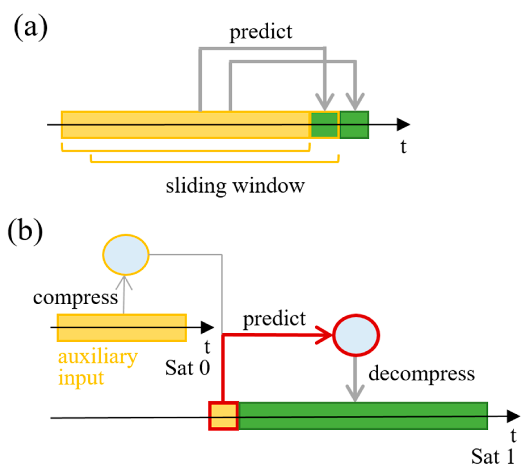
A key finding enabling the CDOP is that the arbitrary tracks of satellites within an LEO constellation, in the form of a time series of the differences between the actual and the coarsely estimated positions, as introduced in the previous subsection, can all be encoded and compressively represented by very few latent features using a single encoder, while introducing negligible reconstruction errors (in orders of tens of meters, see Figure 3). Although compressive autoencoders have been widely used in audio and image compression tasks [26,27,28,29,30], and also in compression of financial and biomedical time series [31,32,33], their application to orbital data with quantified reconstruction errors has not been discussed, and this compressibility is not self-evident. As a result of the condensation in dimensions, the mapping that links the relatively arbitrary (within the constellation) initial states and the latent features representing the predicted orbits can be well learned and established. In contrast to a traditional sliding window framework (Figure 4), the CDOP takes only the initial step and auxiliary information about the reference arc as the input, and outputs the entire predicted time series in one inference.
Figure 3.
reconstructed by the compressive autoencoder. Upper panel: Absolute values of true and reconstructed . Lower panel: Differences between true and reconstructed values.
Figure 4.
Schematic diagrams of (a) a traditional sliding window framework, where the time series inputs (yellow) are mapped to the outputs (green) one step at a time; (b) CDOP framework, where the most important input, the initial condition at the first step, is mapped to a low-dimensional latent vector and then decompressed to get the entire output series.
2.2.1. Dataset
We first create the dataset for training and validating our model. After training, our CDOP model should be able to make 24 h predictions about the corrections to the analytical estimations discussed previously, for arbitrary OP tasks arising from satellites within a chosen LEO constellation and within an extended time period, e.g., a year. Because our method involves at least two satellites within an LEO constellation, and in the current stage it is hard to get enough real-life ephemerides of LEO large-scale constellations with known maneuver schedules, we use a numerical high-precision orbit propagator (HPOP) [34] to generate simulated ephemerides for the dataset in our demonstration. Nevertheless, future real-life ephemerides could be used to train the model following the same methodology in practical applications. For now, our model takes the HPOP-generated orbits with measured or forecasted space weather as the ground truth. Thus, when applying the current model to real-life scenarios, the residue error to a real orbit will be a combination of the residue error reported in this paper and the error inherited from the HPOP/atmospheric model. Naturally, the more precise the HPOP/atmospheric model used to generate the training dataset is, the lower the combined error will be. Our focus here is to reduce the error relative to the high-precision numerical model, whose computation cost is much higher than that of our hybrid model. The HPOP model we use in this study employs a GGM03C gravity model to the 70th degree and 70th order; a JPL-DE440 model with sun, moon and all the planets included; an NRLMSISE-00 atmospheric density model; a conical shadow model for solar radiation pressure; and takes into account the solid Earth tides and ocean tides but no general relativity effects, giving rise to position errors within tens of meters per day [34].
The dataset consists of inputs of the model and the corresponding output labels. For the inputs, in addition to the initial orbital elements, the initial time and space weather indices (we postpone the detailed discussion about the selection of these non-series inputs to the next paragraph and Section 3.2) and three auxiliary time series for improving precision are also included: the J2 mean semimajor axis of the reference arc , the J2 mean argument of latitude of the reference arc and the geodetic height of the reference arc . For the output labels, the analytically estimated for each time step discussed in Section 2.1 is subtracted from the ground truth obtained using the HPOP model introduced above, giving the correction in the ECI frame. To better characterize the time evolution of and decouple the phase (i.e., argument of latitude) error from oscillations in the components of due to the orbital period, we transform into the radial, along-track, cross-track (RTN) frames to get , which is chosen as the output label for our dataset. For simplicity, the transformation to the RTN frame is done by constructing rotation matrices based on the analytically estimated osculating elements , and instead of and .
Now, we discuss further the input features. The initial times and in the modified Julian date (MJD) and the (forecasted) space weather indices of including the AP indices and F10.7 indices, are selected. More importantly, the initial orbital elements or state vectors of and should be the main input features of the model. Nevertheless, there are a variety of equivalent representations that are mutually convertible, including osculating elements, mean elements, state vectors in earth-fixed frame, state vectors in inertial frame, etc. Although the choice of proper input features can be made intuitively, this choice often lacks definite criterion. For example, the state vectors in an earth-centered earth-fixed (ECEF) frame may reflect better the effects of non-spherical gravitation perturbations, while the state vectors in inertial frames are more conventional orbital dynamics representations, since no inertial forces are introduced. To resolve this ambiguity, we adopt a data-driven input feature selection method [35]. This gives the measurable importance of each input feature in making predictions. Specifically, we start from taking all redundant representations as input features to construct and train the model to convergence. Then, a variational dropout layer is added after the input layer. Meanwhile, the following term is added to the loss function:
where is a weight factor and is the original loss function (see Section 2.2.3). is the keep probability of the th input feature, and it is the trainable parameter of the variational dropout layer. The modified model is trained again with all the original parameters fixed and being the only trainable parameter. This adaptively gives the importance (to be precise, the unimportance) of each input feature, signified by the probability the feature can be shut down while not significantly degrading the performance of the model. Based on this knowledge, a modified model with only the important input features will be constructed again and trained to validate the selection.
2.2.2. Model Architecture
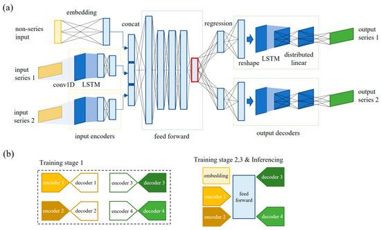
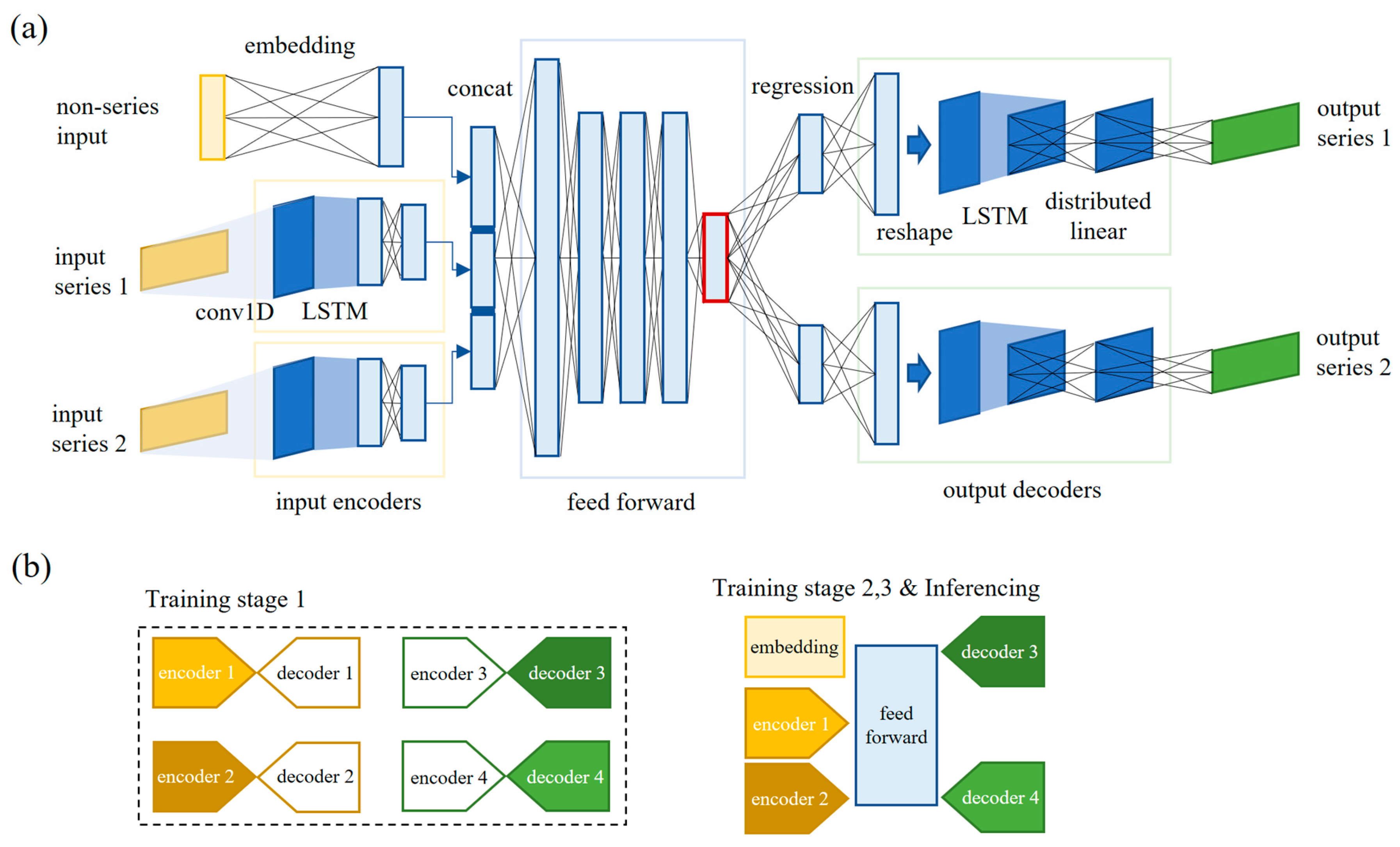
Our CDOP model comprises the following modules (Figure 5): input and embedding layers for the non-series inputs, encoders for the time series inputs, a feed-forward network that maps the inputs to the bottleneck latent features, regression layers transforming the bottleneck latent features into pre-decode features, and finally the decoders.
Figure 5.
(a) Architecture of the CDOP model. The bottleneck layer is highlighted in red. (b) Structure of autoencoders and the correspondences among the encoders and decoders in the CDOP model.
The input encoders and output decoders are first trained in unsupervised learning processes, where autoencoders based on LSTM layers are constructed for each type of input and output time series. Since there will be two auxiliary input time series and two output time series, we correspondingly construct four autoencoders. The schematic structure of each autoencoder is shown in Figure 5b. We group and as one set of two-channel input series, and the geodetic height as the second input series. For the outputs, the radial and normal position error and are grouped into a two-channel output series, with the track error being another output series. The four sets of series correspond to the four autoencoders trained individually. After these autoencoders are trained to convergence, only the encoders for the input series and the decoders for the output series are taken as part of the CDOP model, while the decoders for the input series will not be used again after this point. This allows us to optimize the computational workloads during inferencing by balancing the complexity between the encoders and the decoders when designing the autoencoders. For the output decoders, since their capability to accurately reconstruct the time series strongly affects the final OP precision, the corresponding autoencoders cannot be oversimplified models with very few parameters. Nevertheless, a high-fidelity reconstruction can be achieved by combining strong encoders with small decoders. By integrating the lightweight pre-trained decoder into the CDOP model while leaving the encoder out, precise OP with a low inferencing computational cost is made possible. For the input encoders, since they only need to extract the features rather than recover all the details in the input time series, small-parameter networks that correctly capture the trends and oscillation patterns can be safely used. In brief, the pre-training of the autoencoders keeps the CDOP model lightweight and accurate at the same time.
The bottleneck layer in the CDOP architecture, as highlighted in red in Figure 5a, helps prevent overfitting. Suppose, instead, that we have two fully connected networks, each connecting the post-input encoder layers directly to the two output decoders, respectively. Then, effectively, the prediction of and the prediction of and are decoupled. It is easier for the training to converge but also easier to overfit each output time series because of the decoupling. The bottleneck structure, in comparison, postpones the “branching” until the very last layer, so that the bottleneck latent features have to compose a fused representation of , and , and the main representation–transformational fitting happens only in the last branched regression layers. In short, the bottleneck structure helps the network to learn a mapping that better reflects the dynamics and is less prone to overfitting.
2.2.3. Training
The training is three-staged: First, the encoders and decoders are completed to form autoencoders, which are trained individually in unsupervised learning. Then, the CDOP model is trained in supervised learning, with the parameters of the encoders and decoders loaded and fixed. Since the encoders and decoders are well trained in the first stage of unsupervised learning and can encode/decode time series quite accurately to/from low-dimensional latent representations, their parameters are fixed in this stage in order to avoid unnecessary updates at the beginning of the supervised learning. Finally, all the parameters in the CDOP model are set as trainable and the model is fine-tuned.
In all three training stages, we use an Adam optimizer with the learning rate being 5 × 10⁻⁵. In the first unsupervised training stage, the loss function is simply the MSE loss between the input time series and the output time series. The batch size is 8, and the maximum number of epochs is set to 1000. In the next two training stages, L1 regularization is used to sparsify the parameters of the feed-forward and regression modulus that connect the post-encode features to the pre-decode features. The loss function is
where is the MSE loss between the output time series and the labels, and is the sum of the absolute values of all parameters in the feed-forward and regression modulus. The weight factor is initially 1 × 10⁻⁶ and is multiplied by 0.99 after every 100 training epochs. The batch size is set to 32, and the maximum number of epochs is set to 10,000.
3. Results and Discussion
To demonstrate our method, we consider an LEO Walker constellation. The initial orbital elements of and are set according to Table 1. When constructing the dataset for our neural network model, the initial RAAN of the reference arc and the initial argument of latitude of the reference arc are randomly generated, whereas are randomly chosen within and , in order for to actually be a valid reference for , i.e., to actually share a similar ground track with . Here, 0.99727 is one sidereal day in units of mean solar days. The initial time is randomly taken from the interval 00:00:00 1 January 2023 to 00:00:00 1 January 2024. is any time 24 to 48 h after . The step size of the time series is 60 s, and each time series contains 1440 steps, i.e., lasts 24 h.
Table 1.
Orbital elements of satellites in the datasets.
We create a dataset containing 86,500 randomly generated pairs of and orbital data, divided into a training set with 80,000 pairs, a valid set with 6000 pairs and a test set with 500 pairs. In addition to the dataset containing randomly generated reference arcs as discussed above, we construct five extra test sets by simulating five Walker constellations. Each extra set contains four OP tasks within the constellation, and each OP task will utilize five different referential arcs extracted from the historical ephemerides of the Walker constellation. We design the CDOP model following the guiding principles discussed previously, and the working architecture is tabulated in Table 2. Note that the decoders for the inputs and the encoders for the outputs are only for the first stage of unsupervised learning.
Table 2.
Model parameters of the CDOP model and the autoencoders.
3.1. Performance
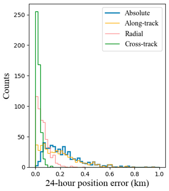
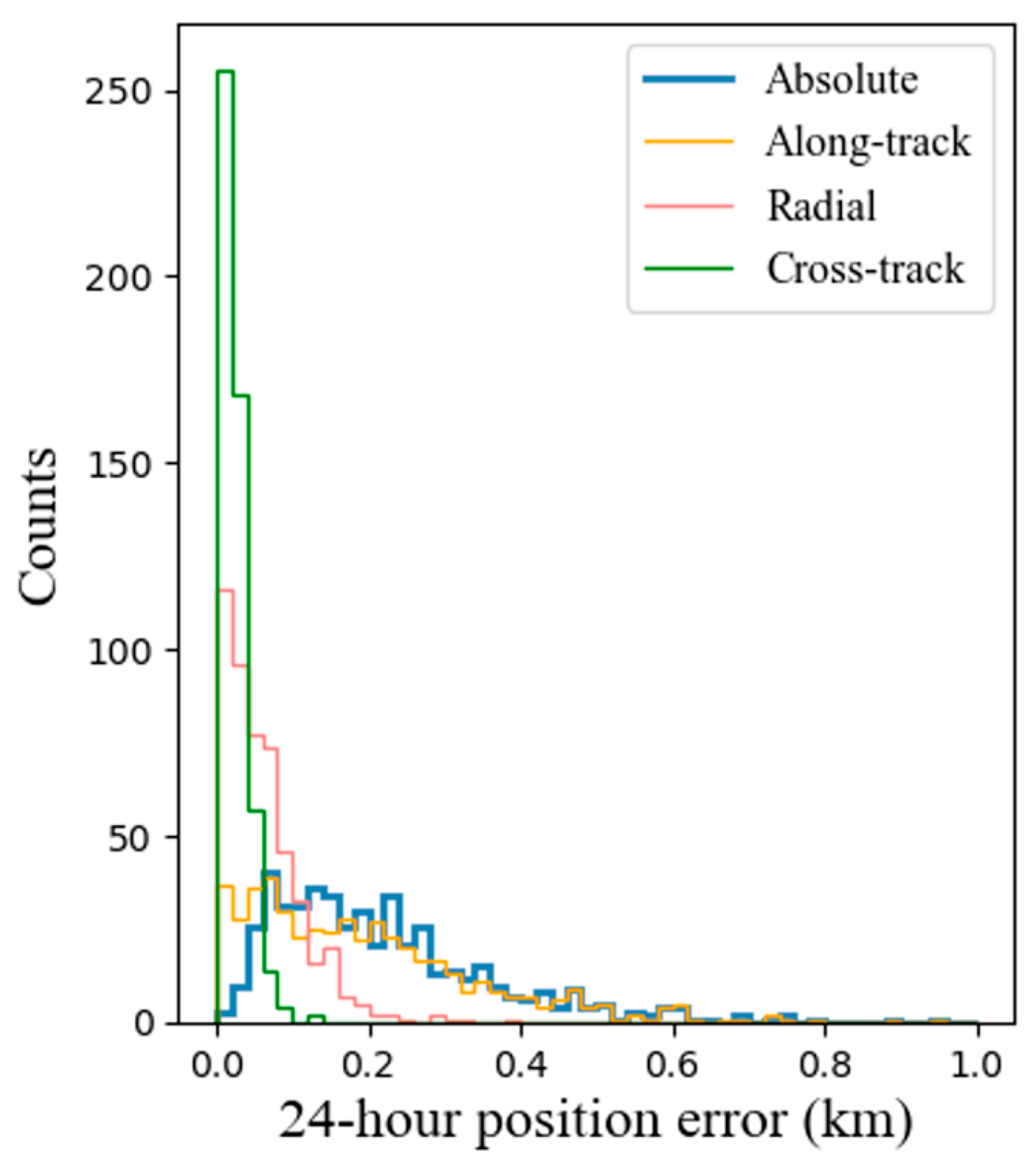
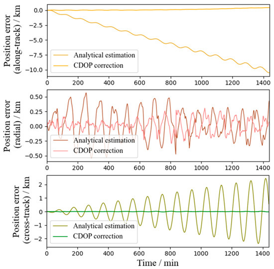
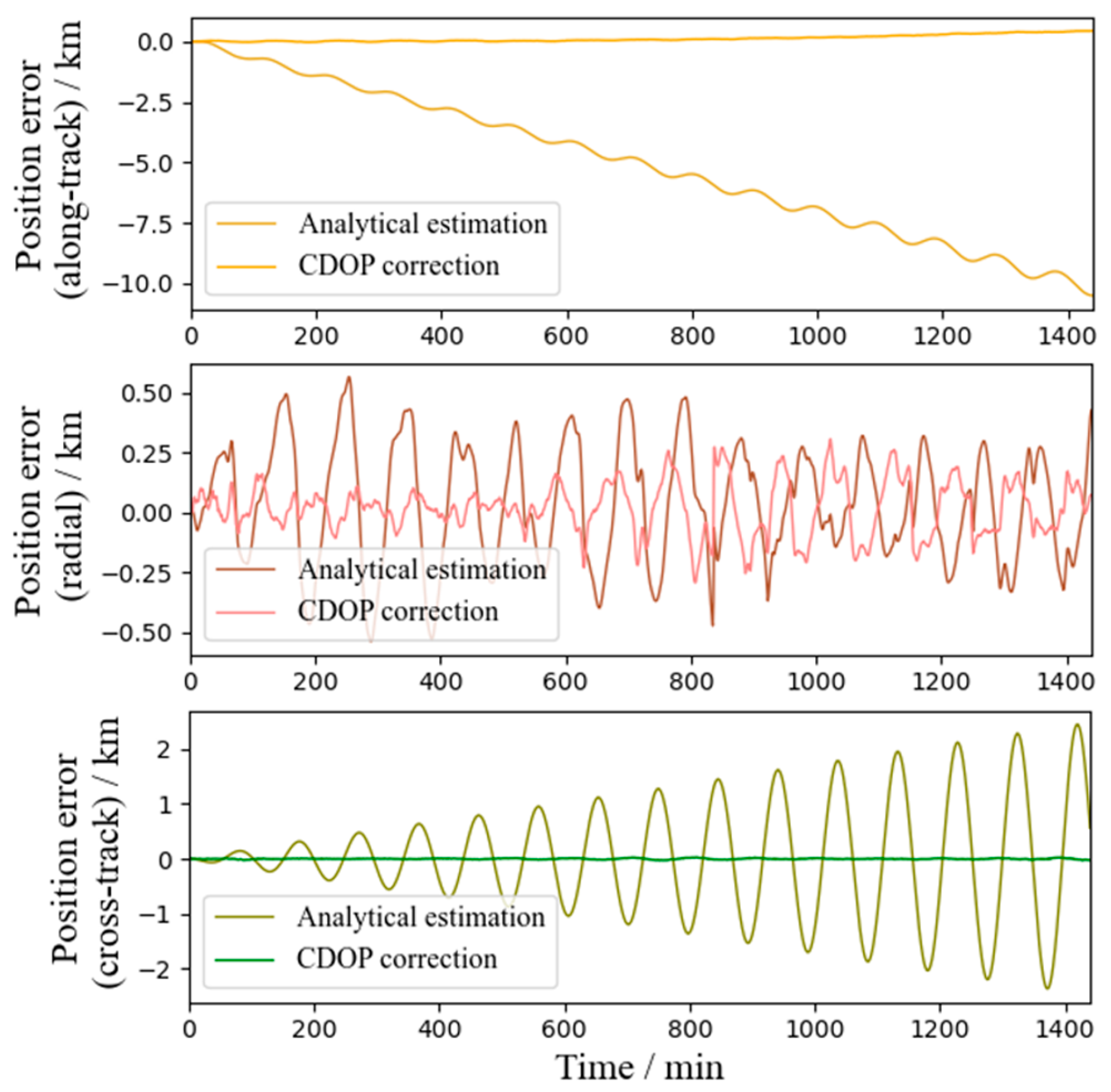
We first test the accuracy of our model taking into account only one reference arc for each OP task on the randomly generated test set containing 500 data entries, which is generated using the same procedure as for the training and valid sets but never used during training. The 24 h residual position error on average (RMSE) is 254 m, 81 m and 29 m for the along-the-track, radial and cross-track components for this test set, and the overall absolute position error is 268 m on average (RMSE). A histogram showing the distribution of each component of the residue error is shown in Figure 6. In 94.4% of cases (close to 2), the overall residue error is less than 500 m, and in 76.6% of cases the error is less than 300 m. In Figure 7 we show a typical time series of the components of the residue error for the 24 h OP, taking a randomly chosen test sample. In comparison, we also show the analytically estimated raw error before using the CDOP model for fine correction. The along-track error is reduced significantly, from 10 km to 400 m, for this sample.
Figure 6.
Distribution of the residue errors on the test set with 500 data entries.
Figure 7.
A 24 h time series of the analytical estimation error and the final residue error on a randomly chosen test sample. The latter is significantly reduced compared to the former for the along-track and cross-track components.
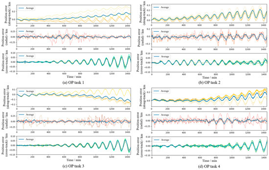
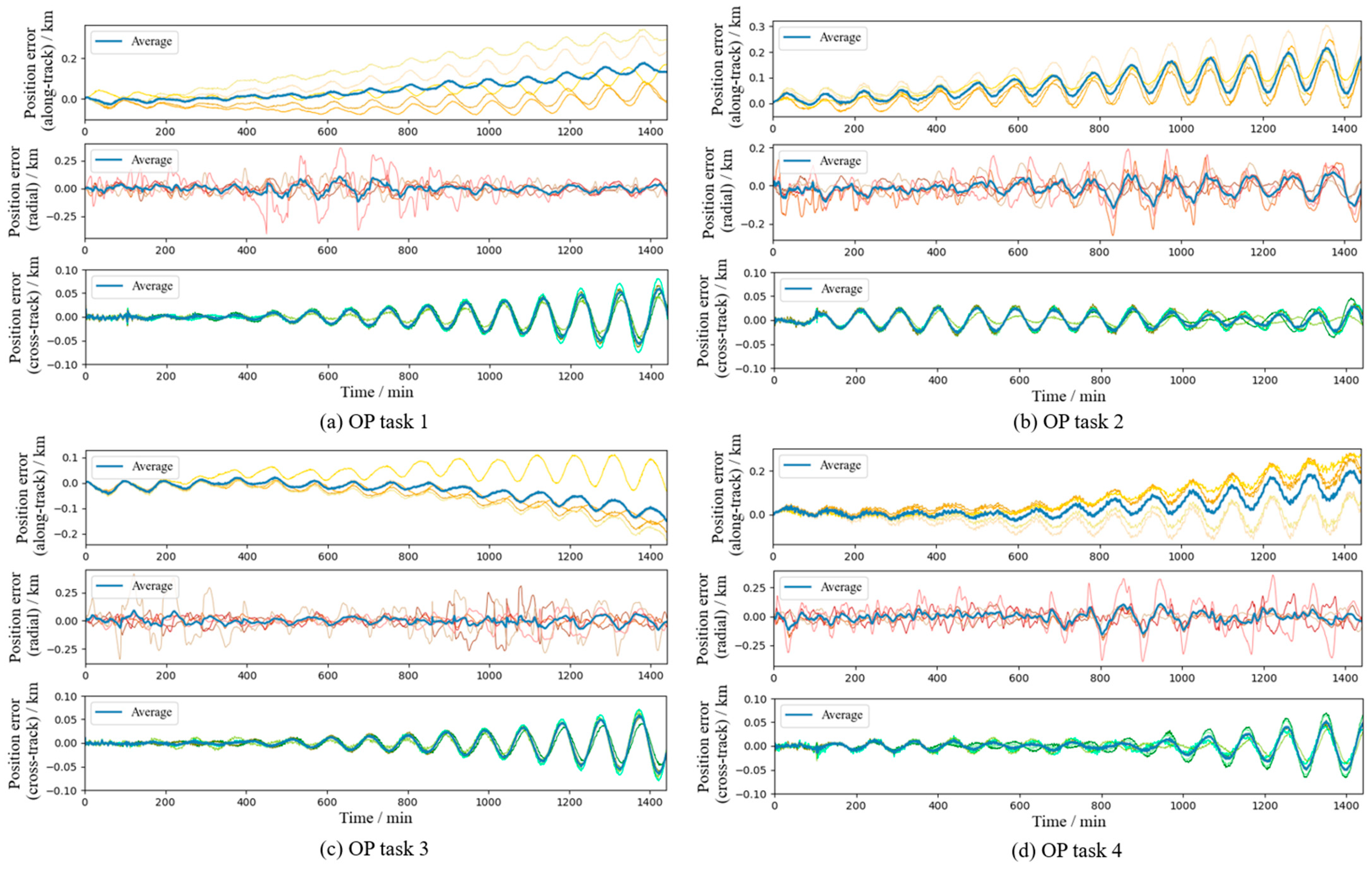
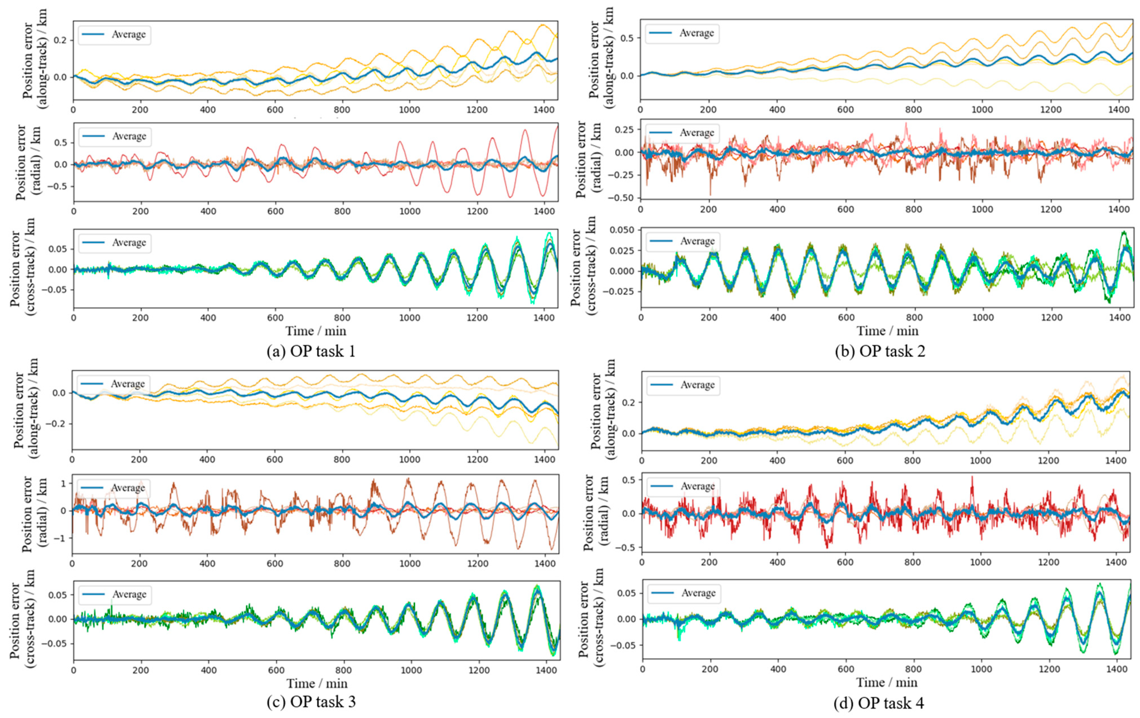
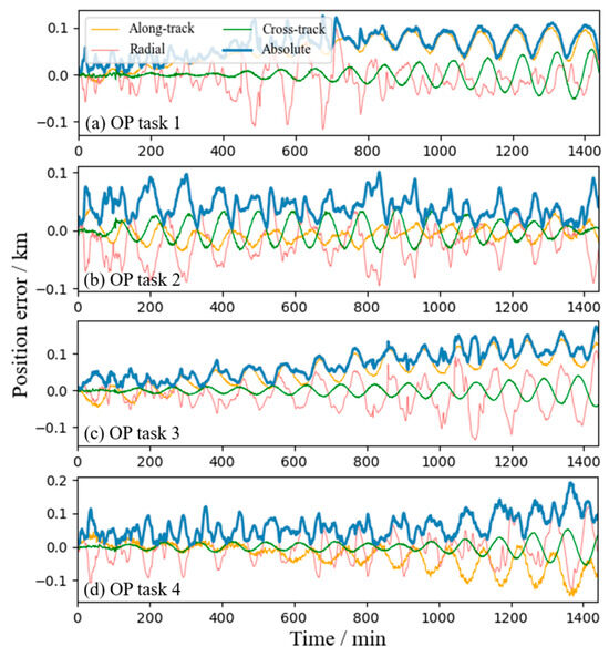
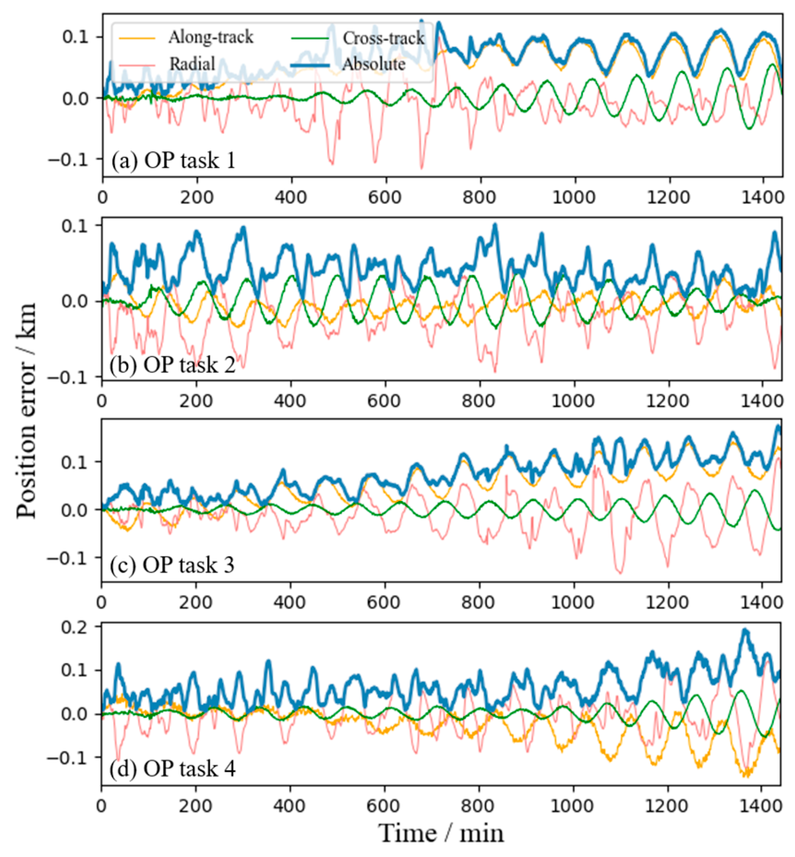
Next, we examine the capability of our model taking into account multiple reference arcs for each OP task on the five extra test sets. For each extra test set, a Walker constellation with a distinct geometry is simulated. For example, in the first extra set, a 400/20/3 Walker constellation is considered. The geometries of the rest of the four extra sets are 375/15/9, 391/23/12, 350/25/11, and 240/30/5, respectively. In each of the simulated Walker constellations, we randomly pick four OP tasks and extract several (five per OP task) historical ephemerides within the same constellation as the reference arcs. Thus, each extra test set contains four to-be-propagated () arcs and 4 × 5 reference () arcs. The scenario time, 1 January 2024 to 4 January 2024, is set to be non-overlapping with that of the training set to better test the generalizability of the model. In Table 3, we list the orbital plane indices p and the in-plane phase indices n of the four to-be-propagated and 20 reference satellites in the first extra test set. Correspondingly, in Figure 8 we show, for each OP task in the first extra test set, the five slightly different predictions due to the five different reference arcs. Similar results for the other four extra test sets are shown in Appendix A. An advantage of our cross-referential framework is that, for each OP task, several reference arcs from different combinations can suppress the statistical fluctuations in individual predictions and further reduce the residue error. This is shown by the thick blue line in Figure 8 and Figures in Appendix A for each extra test set (Figure A1, Figure A3, Figure A5 and Figure A7).
Table 3.
Parameters of the satellites in the 1st extra test set.
Figure 8.
Residue position errors on the 1st extra test set. In each panel, the residue error curves derived from 5 individual reference arcs and another residue error curve derived from averaging over the 5 individual predictions (thick blue) are shown. The average curves show the improved accuracy of the combined prediction.
The maximum residue position error of the 5 × 4 × 5 individual predictions in all the extra test sets reaches 821 m/24 h, and the RMS residue position error is 319 m/24 h, as shown in Table 4. Nevertheless, after we take the arithmetic average over each component of the five predictions, which result from five different reference arcs, to make a combined prediction in each of the 5 × 4 OP tasks, the maximum absolute residue position error is reduced to 332 m/24 h, and the RMS absolute residue position error is reduced to 206 m/24 h. The latter is 35% smaller than the RMS error of all individual predictions. Theoretically, one would expect a reduction by a factor of 2.236 in the RMS error when averaging over five predictions, if these predictions were independent. Since the predictions are for the same OP task, they are surely not independent. Nevertheless, the 35% (1.5-fold) error reduction achieved by aggregating five predictions from different reference arcs is still significant. The accuracy of our model is advantageous when compared with a straightforward sequence-to-sequence LSTM model, as shown in Appendix B.
Table 4.
The 24 h maximum residue position errors for individual/combined predictions on the 5 extra test sets.
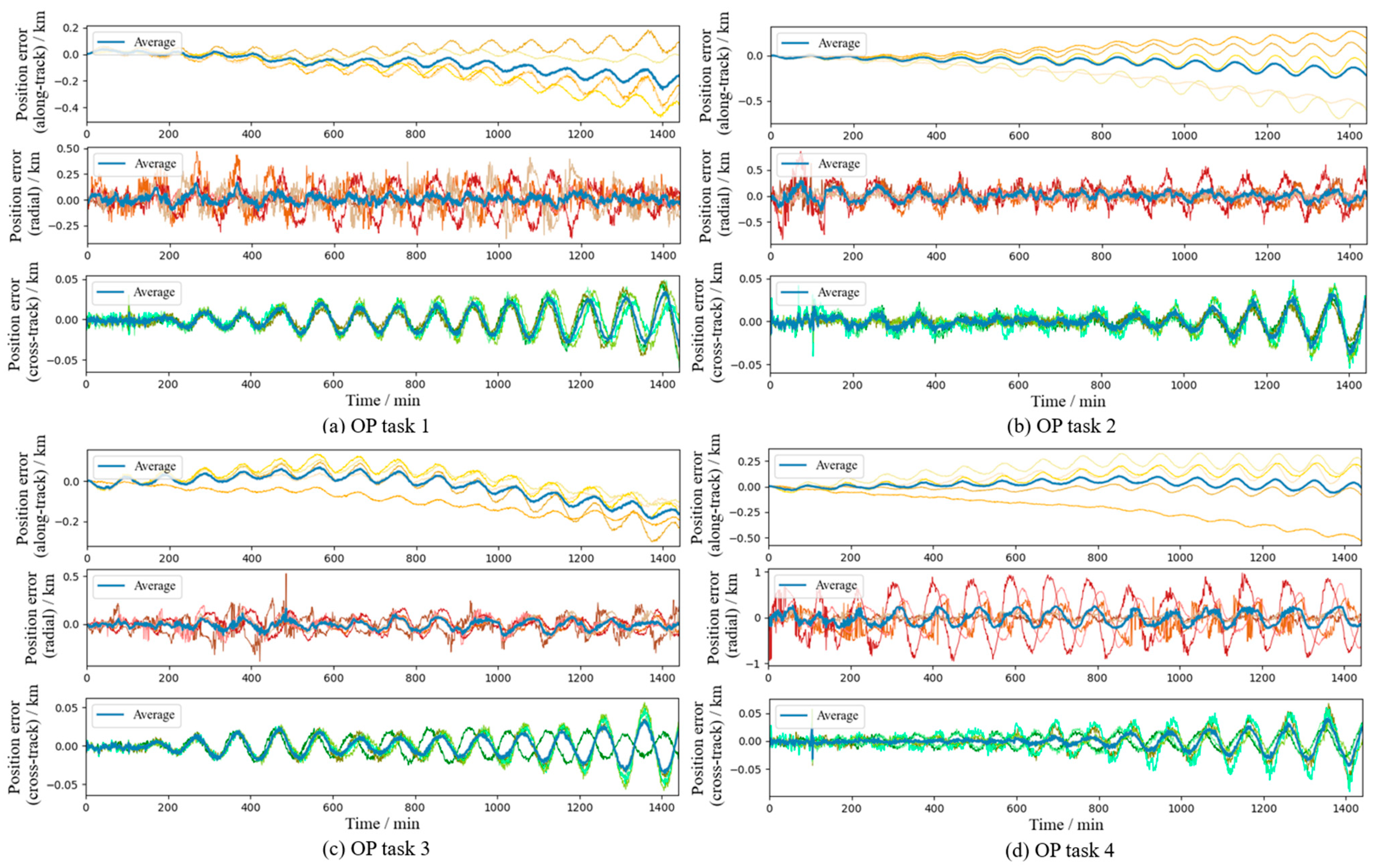
So far, we have assumed that the reference arcs are of high precision (accessed through regular ground uploads). In the case that high-precision historical ephemerides are unavailable when an OP task is initiated, the GNSS telemetry data stored onboard other satellites in the constellation can be shared via inter-satellite links and serve as references. Motivated by this scenario, we examine the performance of the model using “noisy” reference arcs. The input reference arcs in the five extra test sets are added with Gaussian noise of position standard deviation and velocity standard deviation m/s at every time step, corresponding to typical GNSS accuracy in LEO orbits. The errors of the individual and combined predictions resulting from these noisy reference arcs in the first extra test set are shown in Figure 9. Similar results for the other four extra test sets are shown in Figure in Appendix A for each extra test set (Figure A2, Figure A4, Figure A6 and Figure A8). In Table 5, the statistics for the residue position errors using the noisy inputs are shown. The maximum residue position error and the RMS residue position error for the combined predictions mildly increase to 477 m and 283 m, respectively. Although the residue errors increase as GNSS errors in the input reference arcs are introduced, the proposed OP method still works, with a consistent accuracy within 500 m/24 h.
Figure 9.
Residue position errors of individual (thin) and combined (thick blue) predictions using noisy reference arcs on the 1st extra test set.
Table 5.
The 24 h maximum residue position errors for the individual/combined predictions using noisy reference arcs on the 5 extra test sets.
From Figure 8 and Figure 9 and Appendix A, one can see that the five individual predictions using different reference arcs for the same OP task are correlated. Specifically, the position errors often share similar peak-and-valley patterns. This correlation, in principle, may enable detection of accidental mistakes in reference arc inputs, e.g., wrongly selected or missing reference arcs. However, since the number of reference arcs used in one OP task is few (five in our case), common statistical methods can hardly be applied. The ability of the model to perform this error detection remains an open question for us to investigate in the future.
Our CDOP model has 443,151 parameters and 45,764 zero parameters due to the L1 regularization. The inference computational cost of the model is 0.868 MFLOPs. It takes a single core of a 2.30 GHz CPU 20 ms (averaged over 100 runs) to finish one prediction. By comparison, a reduced dynamic integration-based numerical method (see Appendix C), purposely optimized for onboard application, takes 3.5 s to propagate 24 h under the same test environment. This numerical method achieves an accuracy of 200 m/24 h for the position error, which is of the same order as our CDOP method when averaged over five predictions. As another benchmark, the MATLAB HPOP [34] (using MATLAB R2023a) takes 53.8 s to propagate 24 h (N_Step = 1440) under its default setting and the same test environment. Therefore, our method is more than 30 times faster than the integration-based numerical method.
Regarding the data exchange and onboard storage requirements imposed by the cross-referential workflow, each reference arc, including epoch time, 24 h state vectors and geodetic coordinates, comprises 42 kB data. For a constellation (or a sub-shell of a mega constellation) with 1000 satellites, the overall historical reference ephemerides take up 42 MB per day. This can be easily handled by the onboard storage (typically hundreds of GBs), ground TT &C links (typically 10 Mbps) and inter-satellite links (more than a hundred Mbps for RF links).
3.2. Input Feature Analysis
In this subsection, we discuss the results of the non-series input feature selection for our CDOP model. The original redundant non-series input contains 73 features, as listed in Table 6. Here, is in a modified Julian date and is the hour–min–sec corresponding to in UTC. The space weather indices include 3 h AP indices at various time before , as well as daily and 81-day F10.7 indices.
Table 6.
Non-series input features of the CDOP model.
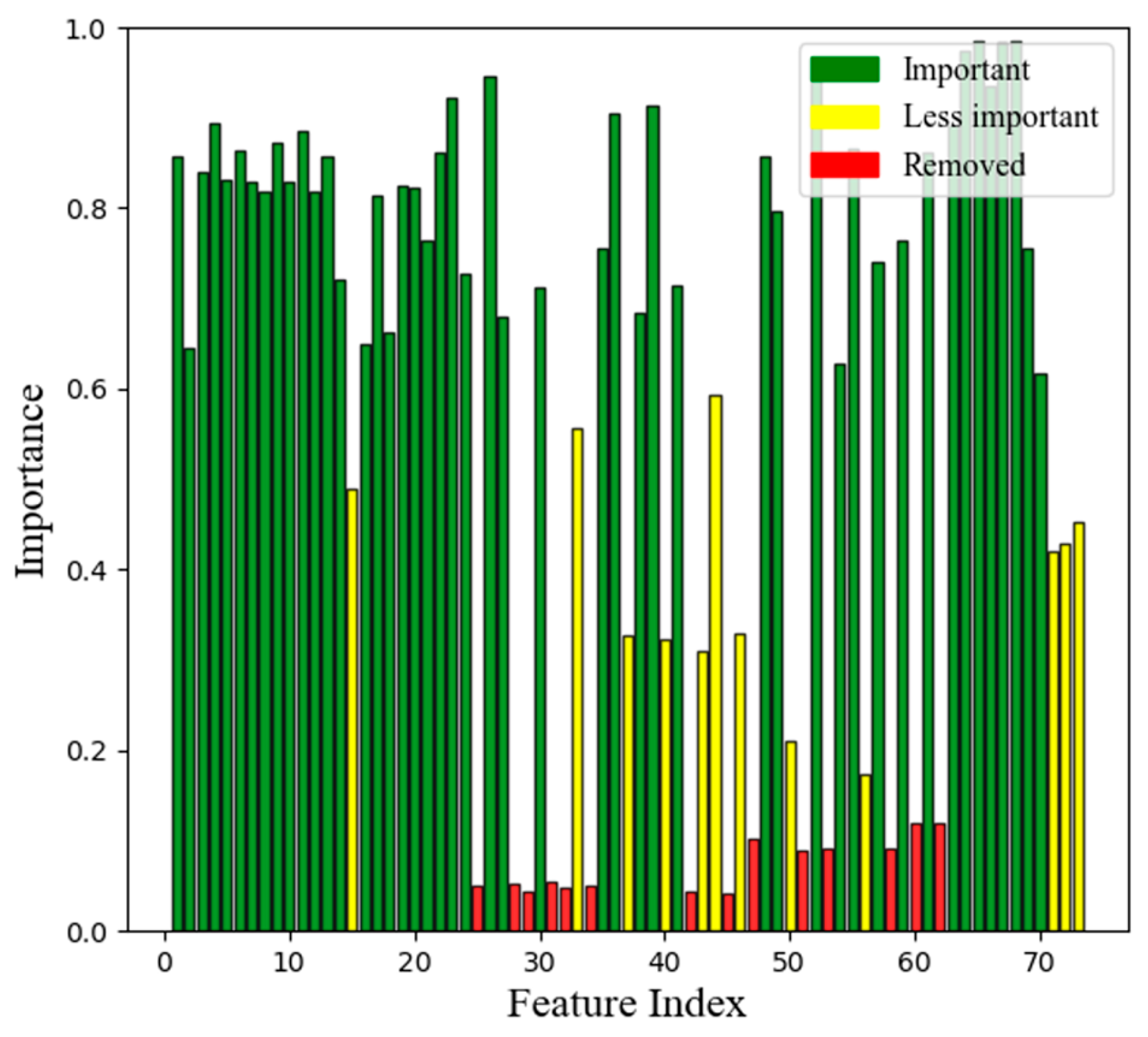
We use the dropout feature selection method, as discussed in Section 2.2.1, to identify those input features that can be excluded while not affecting the accuracy significantly; in other words, those that are unimportant. The keep probability , signifying the importance of each input feature, rated from 0 to 1, is shown in Figure 10. Out of the original 73 input features, 14 features have keep probabilities less than 0.15, which we highlight in red color. The physical meanings of these unimportant features are listed in the rightmost column of Table 6. We see that the unimportant features are indeed redundant representations of the initial states of and . For example, the z-component of the position vector, latitude and argument of latitude (the sum of argument of perigee and true anomaly) all provide almost the same information; thus, only the last one of the three is labeled important and kept. Nevertheless, we also note that the model benefits from some redundant representations. For example, the keep probabilities for both the velocity in the ECEF frame and the Keplerian mean elements are high, resulting in more input features kept than in a minimum irreducible set, allowing the model to achieve better accuracy.
Figure 10.
Keep probability of all 73 input features. Red bars correspond to keep probability less than 0.15, corresponding to removed input features in updated CDOP model.
After removing the 14 least important input features as listed in Table 6 and Figure 10, we construct and train our final CDOP model using the same hyperparameters as in Table 2. This model, with less redundant input features, achieves slightly improved accuracy, with the maximum residual error being 200 m/24 h on the first extra test set (Figure 11).
Figure 11.
Residue position errors (combined predictions averaged over 5 inferences) for the model with truncated input features on the 1st extra test set.
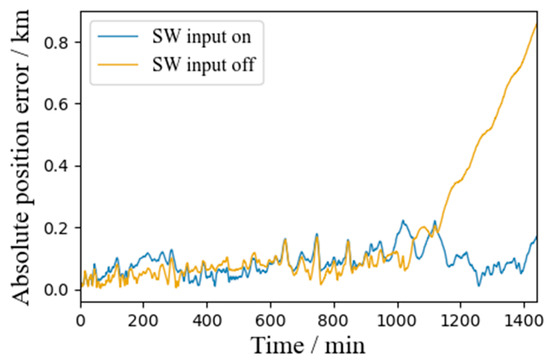
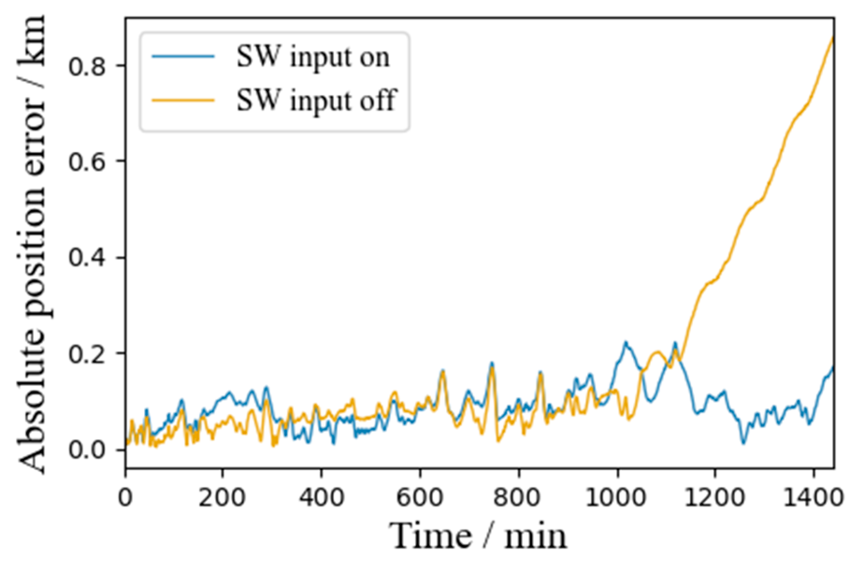
Finally, we test the performance of our model under the condition where the space weather deviates dramatically from the forecasted space weather used in the training. We take the magnetic storm event that occurred on 23–24 April 2023 as the test playground. On these dates, the AP indices exceeded 100, and we turn off (set to zero) all the space weather-related inputs (index 5–22) of our model to make a prediction. The resulting residue error curve is shown in Figure 12. Since the space weather indices are quite important input features, as shown in Figure 10, we expect that there will be a significant degradation in accuracy once these inputs are turned off. Indeed, the residue error rises from 200 m to 800 m. Nevertheless, for the first few hours the prediction with the space weather indices turned off is quite accurate, and since HPOP can give daily position errors of up to a few kilometers for LEO satellites affected by magnetic storms, the result here hints that our cross-referential method may still be advantageous. In principle, the reference arc has already captured the influence due to the anomalous atmospheric drag while the correct space weather indices are yet unavailable in explicit forms, and our method can incorporate this influence into the prediction. This potential is a direction for us to further investigate in the future.
Figure 12.
Comparison of residue error between predictions with space weather-related inputs turned off/on in the presence of magnetic storms.
4. Conclusions
In this work, we introduce a hybrid analytical data-driven orbital propagation method featuring a cross-referential workflow for autonomous optical link acquisition in large-scale satellite constellations. The proposed method aims to improve accuracy and reliability by taking into account multiple reference orbits when making predictions, and to enhance generalizability by a compressive decoder architecture. The main conclusions are drawn as follows:
- (1)
- An analytical transformation considering only the J2 perturbation is sufficient to convert historical ephemerides of satellites in a large-scale constellation into references for OP tasks of other satellites in the same constellation. Further corrections can be made upon this transformed orbit by our neural network model to obtain accurate final propagations.
- (2)
- The position errors of the coarse-grained estimations, obtained from the previous analytical transformation, can be compressed into very low-dimensional latent feature vectors by autoencoders. In our demonstration, an arbitrary 1440-step (24 h) 3-dimensional position error time series in the LEO Walker constellation can be represented by a 24-dimensional latent vector. This significant reduction in dimensions further enables a mapping that better captures the orbital dynamics and has less overfitting to be established.
- (3)
- By aggregating multiple individual predictions using different reference arcs, the statistical fluctuations in individual predictions are suppressed and the residue error of the combined prediction is significantly reduced. The proposed cross-referential OP method can achieve 200 m/24 h accuracy on average while being consistently reliable for the different initial conditions spanning a year. Moreover, the proposed method is lightweight in memory and computational cost, and is 30 times faster than the integration-based numerical method. The overall performance of the proposed method is satisfactory for onboard autonomous link acquisition application.
Author Contributions
Conceptualization, Y.C., R.Z. and C.G.; methodology, Y.C., S.W. and R.Z.; software, Y.C. and K.Y.; formal analysis, Y.C. and S.W.; resources, Z.Y., K.Y. and C.G.; writing—original draft preparation, Y.C. and R.Z.; writing—review and editing, Y.C., Z.Y., S.W., R.Z., K.Y. and C.G.; visualization, Y.C.; supervision, Z.Y. and C.G.; project administration, Z.Y. and C.G.; funding acquisition, Z.Y. and C.G. All authors have read and agreed to the published version of the manuscript.
Funding
This research was funded by the Strategic Priority Research Program of the Chinese Academy of Sciences (Category A): XDA0360404; Outstanding Program of the Youth Innovation Promotion Association of the Chinese Academy of Sciences: Y2023080; Shanghai Oriental Talents Program—Leading Talent Project: LJ2025056; and Shanghai Science and Intelligence “Hundred Teams, Hundred Projects” Program: RZ-RGZN-01-25-0951.
Data Availability Statement
The raw data supporting the conclusions of this article will be made available by the authors on request.
Conflicts of Interest
The authors declare no conflicts of interest.
Abbreviations
The following abbreviations are used in this manuscript:
| OP | Orbit propagation |
| CDOP | Compressive decoder for orbit propagation |
| LEO | Low Earth orbit |
| MEO | Medium Earth orbit |
| SGP4 | Simplified general perturbations 4 |
| HPOP | High-precision orbit propagator |
| LSTM | Long short-term memory |
| BiLSTM | Bidirectional long short-term memory |
| SVM | Support vector machine |
| CNN | Convolutional neural network |
| GRU | Gate recurrent unit |
| GBDT | Gradient-boosting decision tree |
| XGBoost | Extreme gradient boosting |
| ECI | Earth-centered inertial |
| ECEF | Earth centered Earth fixed |
| RTN | Radial, transverse, normal |
| RMSE | Root mean squared error |
| MAE | Mean absolute error |
| SW | Space weather |
| TT &C | Telemetry, tracking and command |
Appendix A. Results for Extra Test Sets 2–5
In this appendix we show, for the second to fifth extra test sets, the (random) choice of reference and propagated satellites in Table A1, Table A2, Table A3 and Table A4, and the residue errors of the predictions.
Table A1.
Parameters of the satellites in the 2nd extra test set from a 375/15/9 Walker constellation.
Figure A1.
Residue position errors of individual (thin) and combined (thick blue) predictions using precise reference arcs on the 2nd extra test set.
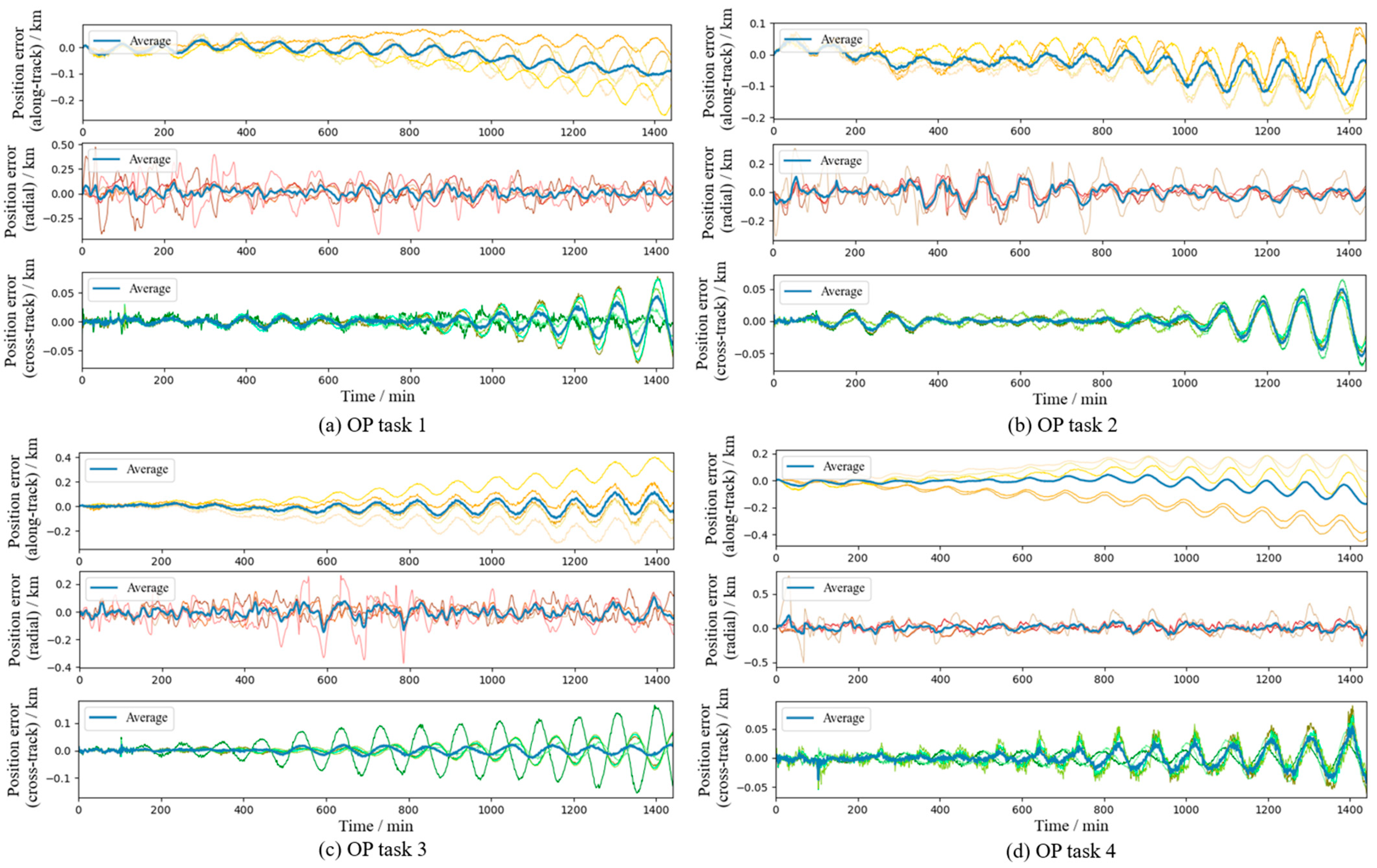
Figure A2.
Residue position errors of individual (thin) and combined (thick blue) predictions using noisy reference arcs on the 2nd extra test set.
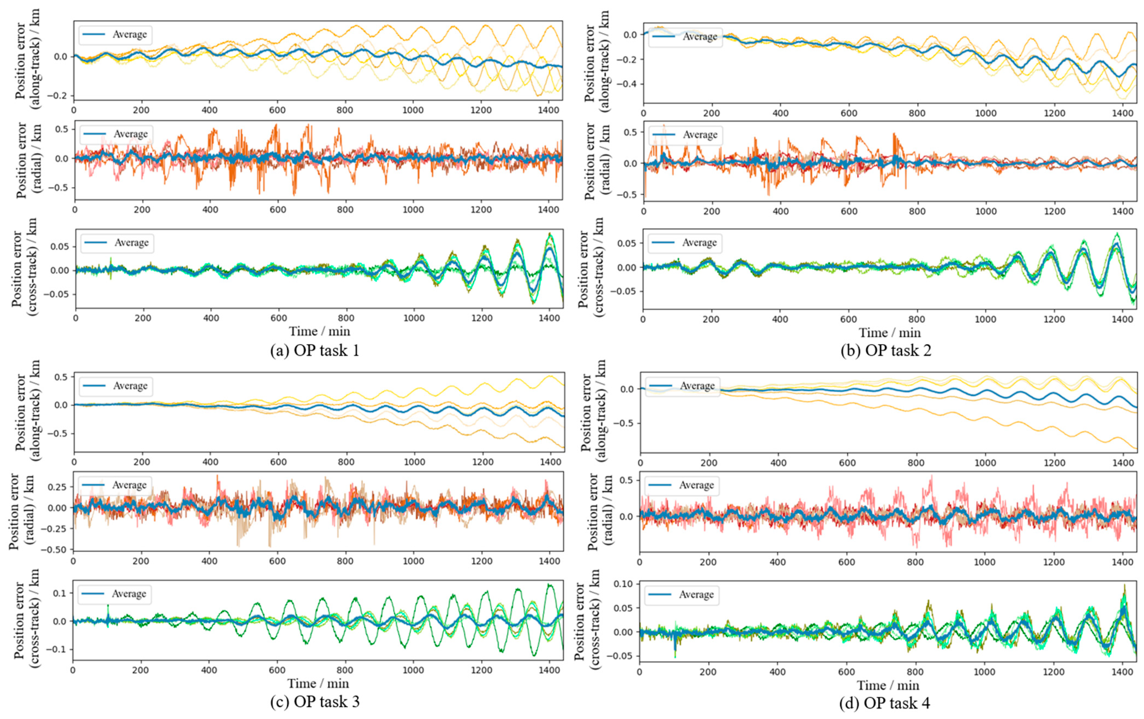
Table A2.
Parameters of the satellites in the 3rd extra test set from a 391/23/12 Walker constellation.
Figure A3.
Residue position errors of individual (thin) and combined (thick blue) predictions using precise reference arcs on the 3rd extra test set.
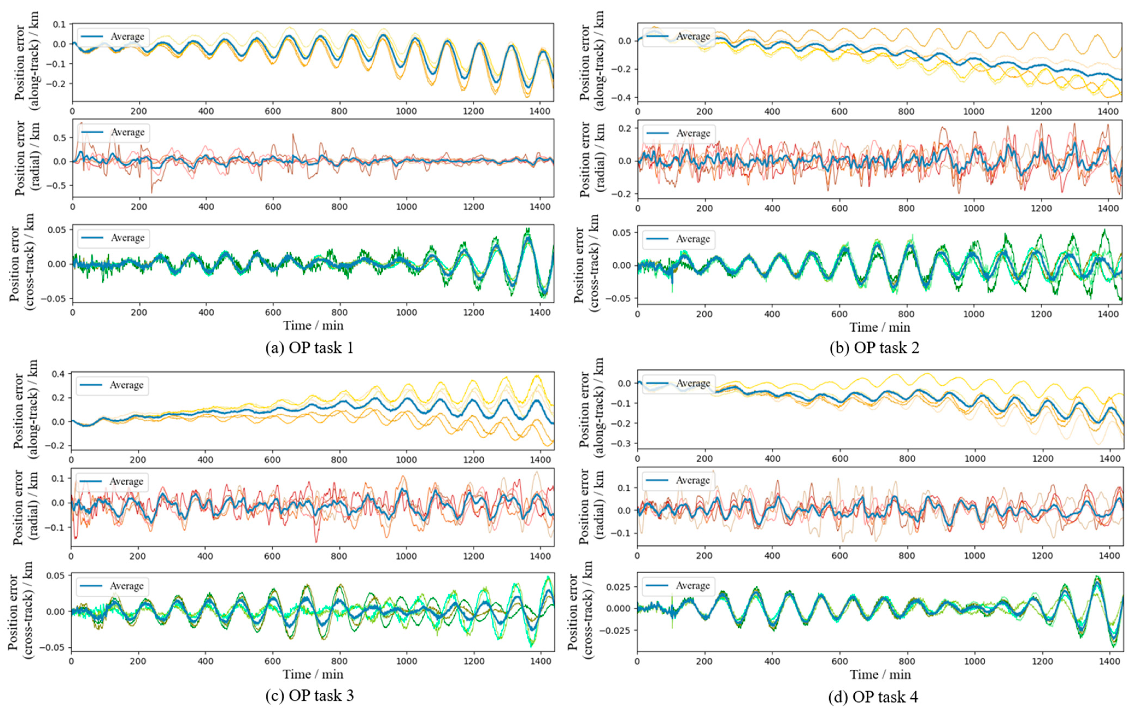
Figure A4.
Residue position errors of individual (thin) and combined (thick blue) predictions using noisy reference arcs on the 3rd extra test set.
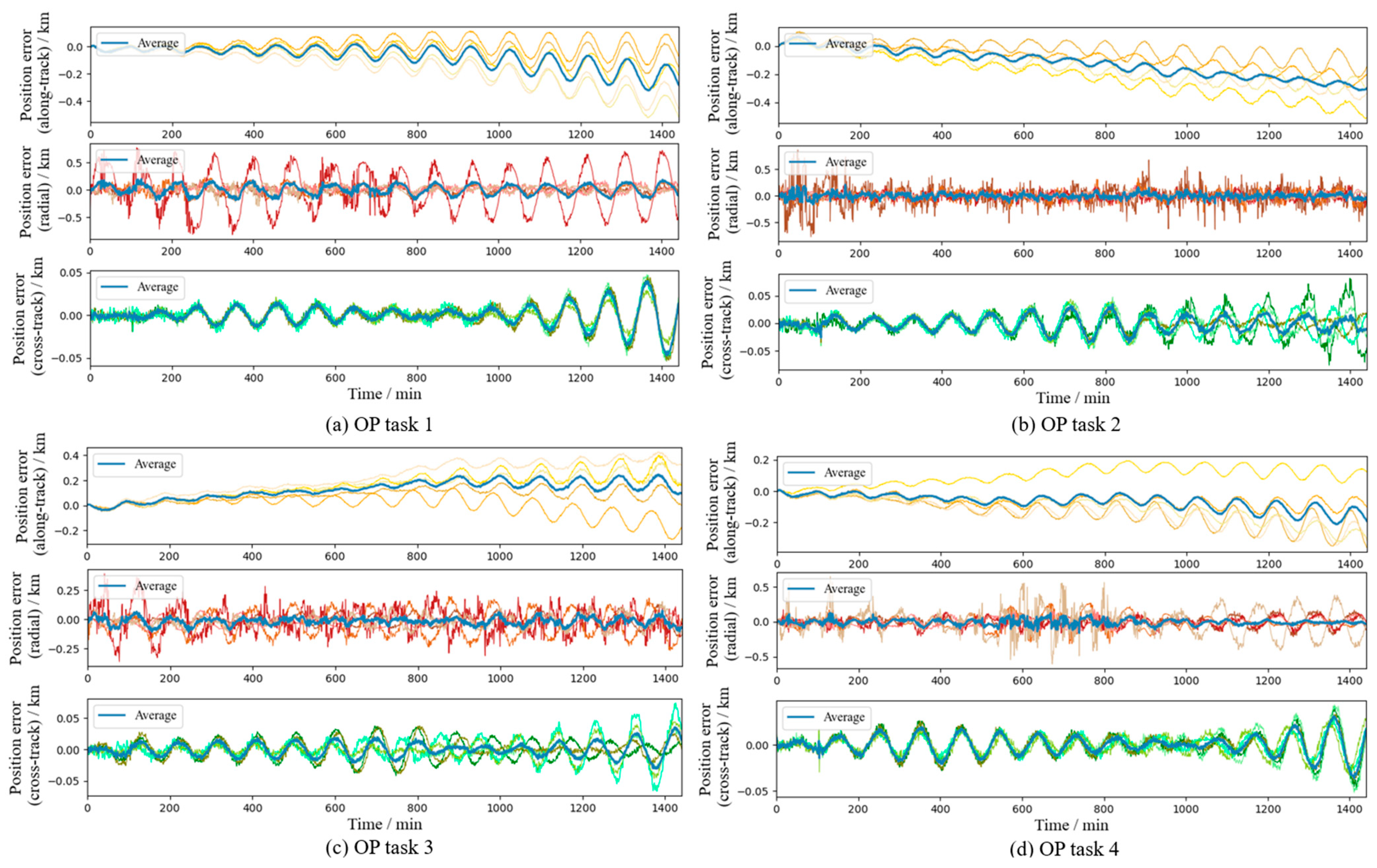
Table A3.
Parameters of the satellites in the 4th extra test set from a 350/25/11 Walker constellation.
Figure A5.
Residue position errors of individual (thin) and combined (thick blue) predictions using precise reference arcs on the 4th extra test set.
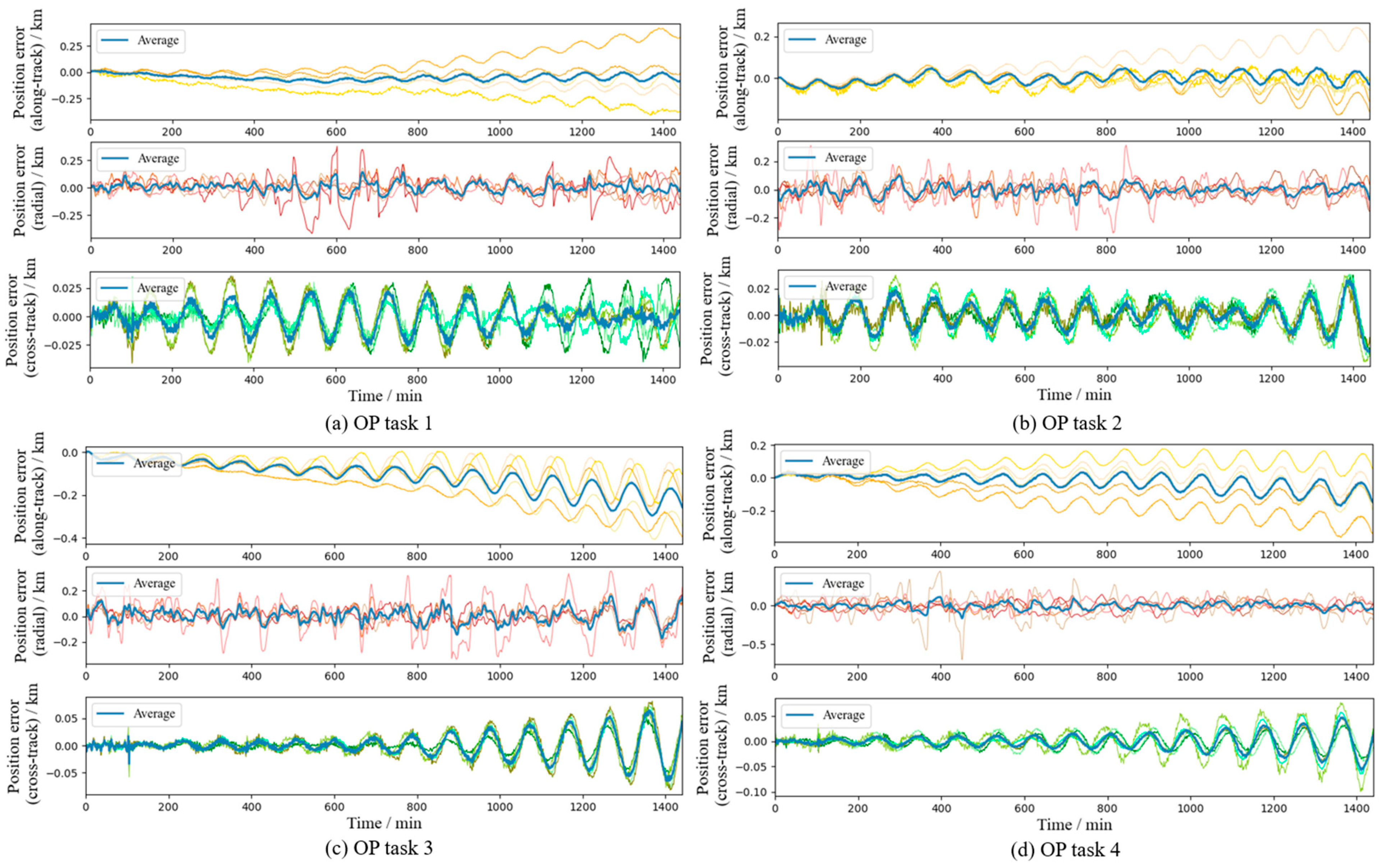
Figure A6.
Residue position errors of individual (thin) and combined (thick blue) predictions using noisy reference arcs on the 4th extra test set.
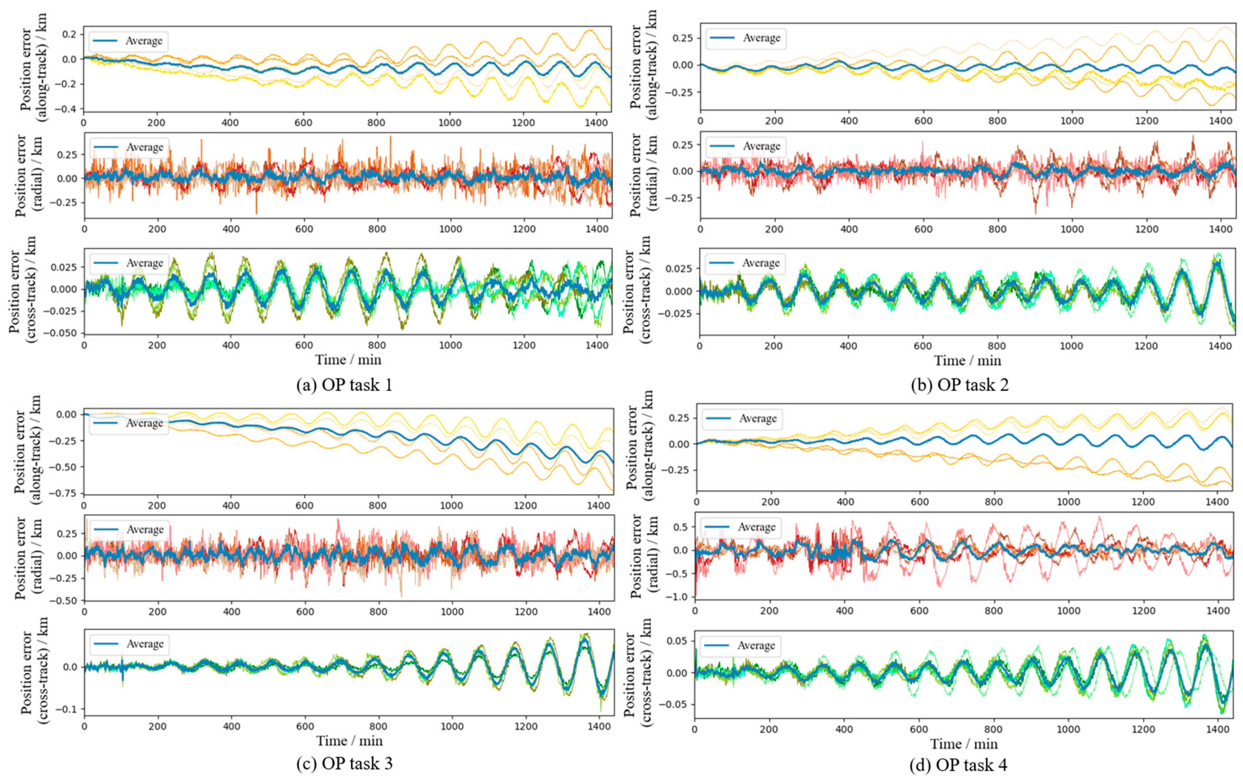
Table A4.
Parameters of the satellites in the 5th extra test set from a 240/30/5 Walker constellation.
Figure A7.
Residue position errors of individual (thin) and combined (thick blue) predictions using precise reference arcs on the 5th extra test set.
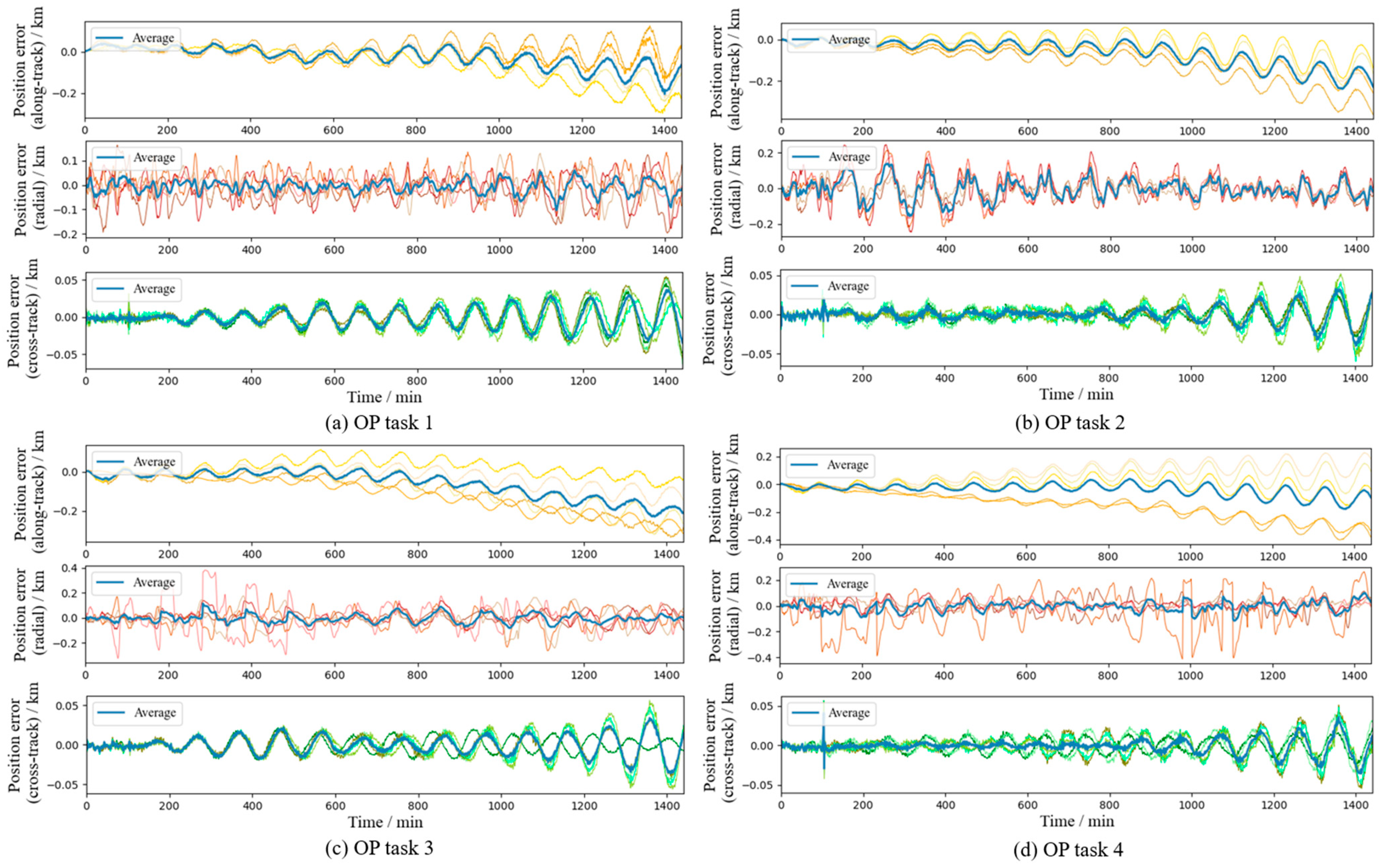
Figure A8.
Residue position errors of individual (thin) and combined (thick blue) predictions using noisy reference arcs on the 5th extra test set.
Appendix B. Straightforward Sequence-to-Sequence LSTM Model
In this appendix, the performance of a benchmarking sequence-to-sequence LSTM model is shown. The straightforward LSTM model takes the same inputs as our CDOP model, i.e., a time series input with three features and a static input vector with 73 features, and outputs the correction to the position estimation in an RTN frame. The straightforward LSTM model first broadcasts the static input to every time step, forming sequential inputs with 76 features. Then, two LSTM layers with hidden_size = 64 follows. Finally, a time-distributed linear output layer is applied. The model is trained using an Adam optimizer and MSE loss function on the same training and validation sets as our CDOP model. The batch size is set to 32 and the learning rate is set to 0.0001. The maximum epoch number is set to 1000.
In Table A5, we show the residue position errors of the straightforward LSTM model for 100 individual predictions using precise reference arcs on the five extra test sets. In Table A6, we show the residue position errors of the straightforward LSTM model for the 100 individual predictions using noisy reference arcs on the five extra test sets. All the absolute errors are significantly larger than those of our CDOP model.
Table A5.
The 24 h maximum residue position errors of the straightforward LSTM model for individual predictions on the 5 extra test sets.
Table A6.
The 24 h maximum residue position errors of the straightforward LSTM model for individual predictions using noisy reference arcs on the 5 extra test sets.
Appendix C. Reduced Dynamic Integration-Based Method
The reduced dynamic integration-based OP method we compare our model to is based on HPOP, but uses simplified perturbation force models. Its employs an RKF78 integrator and takes into account the following perturbations:
- Non-spherical Earth gravity: GGM03C model to the 10th degree.
- Third-body gravity: Uses the analytical ephemerides in Standish (1992) [36], taking into account the sun and the moon.
- Solid tide: To the second order, using the following analytical potential:
- Atmospheric drag: Use the following exponential atmospheric density model:
and are the solar right ascension and the solar declination, respectively.
- Solar radiation pressure: Use the cylindrical shadow model.
The reduced dynamic model is implemented in C++. The integration step is set to 20 s, and propagated for 1 day when comparing it with our proposed method.
References
- Lee, K.; Mai, V.; Kim, H. Acquisition Time in Laser Inter-Satellite Link Under Satellite Vibrations. IEEE Photonics J. 2023, 15, 7303009. [Google Scholar] [CrossRef] [Scilit]
- Yin, Z.S.; Wu, C.H.; Guo, C.B.; Li, Y.C.; Xu, M.W.; Gao, W.W.; Chi, C.X. A comprehensive survey of orbital edge computing: Systems, applications, and algorithms. Chin. J. Aeronaut. 2025, 38, 103316. [Google Scholar]
- He, S.Y.; Wu, C.H.; Guo, C.B. Enhancing space-air communication through anomaly detection in LEO satellite constellations and low-altitude aircraft networks using graph representation learning. Sci. China Technol. Sci. 2026, 69, 100308. [Google Scholar]
- Wu, C.H.; Guo, C.B.; Yin, Z.S. A Distributed-Computing Architecture for Enabling In-Orbit Satellite Adaptation to Evolving AI Models. IEEE Internet Things J. 2025, 13, 3513–3528. [Google Scholar]
- Levit, C.; Marshall, W. Improved orbit predictions using two-line elements. Adv. Space Res. 2011, 47, 1107–1115. [Google Scholar] [CrossRef] [Scilit]
- Bennett, J.C.; Sang, J.; Smith, C.H.; Zhang, K. Improving low-earth orbit predictions using two-line element data with bias correction. In Advanced Maui Optical and Space Surveillance Technologies Conference; AAS: Kihei, HI, USA, 2012; Volume 1, p. 46. [Google Scholar]
- San-Juan, J.F.; Perez, I.; San-Martin, M.; Vergara, E.P. Hybrid SGP4 orbit propagator. Acta Astronaut. 2017, 137, 254–260. [Google Scholar] [CrossRef] [Scilit]
- Bai, X.Z.; Chen, L.; Tang, G.J. Periodicity characterization of orbital prediction error and Poisson series fitting. Adv. Space Res. 2012, 50, 560–575. [Google Scholar] [CrossRef] [Scilit]
- Peng, H.; Bai, X.L. Improving orbit prediction accuracy through supervised machine learning. Adv. Space Res. 2018, 61, 2628–2646. [Google Scholar] [CrossRef] [Scilit]
- Peng, H.; Bai, X.L. Exploring capability of support vector machine for improving satellite orbit prediction accuracy. J. Aerosp. Inf. Syst. 2018, 15, 366–381. [Google Scholar] [CrossRef] [Scilit]
- Peng, H.; Bai, X.L. Obtain confidence interval for the machine learning approach to improve orbit prediction accuracy. In AAS/AIAA Astrodynamics Specialist Conference; AAS/AIAA: Snowbird, UT, USA, 2018; pp. 2131–2147. [Google Scholar]
- Peng, H.; Bai, X.L. Gaussian processes for improving orbit prediction accuracy. Acta Astronaut. 2019, 161, 44–56. [Google Scholar] [CrossRef] [Scilit]
- Peng, H.; Bai, X.L. Artificial neural network-based machine learning approach to improve orbit prediction accuracy. J. Spacecr. Rocket. 2018, 55, 1248–1260. [Google Scholar]
- Peng, H.; Bai, X.L. Comparative evaluation of three machine learning algorithms on improving orbit prediction accuracy. Astrodynamics 2019, 3, 325–343. [Google Scholar] [CrossRef] [Scilit]
- Peng, H.; Bai, X.L. Limits of machine learning approach on improving orbit prediction accuracy using support vector machine. In Proceedings of the Advanced Maui Optical and Space Surveillance Technologies Conference, Maui, HI, USA, 19–22 September 2017; p. 15. [Google Scholar]
- Izzo, D.; Märtens, M.; Pan, B. A survey on artificial intelligence trends in spacecraft guidance dynamics and control. Astrodynamics 2019, 3, 287–299. [Google Scholar] [CrossRef] [Scilit]
- Xopoшилoв, C.B.; Peдькa, M.O. Deep learning for spacecraft guidance, navigation, and control. Kocмiчнa нaукa i meхнoлoгiя 2021, 27, 038–052. [Google Scholar] [CrossRef] [Scilit]
- Silvestrini, S.; Lavagna, M. Deep learning and artificial neural networks for spacecraft dynamics, navigation and control. Drones 2022, 6, 270. [Google Scholar] [CrossRef] [Scilit]
- Li, B.; Huang, J.; Feng, Y.M.; Wang, F.H.; Sang, J.Z. A machine learning-based approach for improved orbit predictions of LEO space debris with sparse tracking data from a single station. IEEE Trans. Aerosp. Electron. Syst. 2020, 56, 4253–4268. [Google Scholar] [CrossRef] [Scilit]
- Li, B.; Zhang, Y.; Huang, J.; Sang, J. Improved orbit predictions using two-line elements through error pattern mining and transferring. Acta Astronaut. 2021, 188, 405–415. [Google Scholar] [CrossRef] [Scilit]
- Curzi, G.; Modenini, D.; Tortora, P. Two-line-element propagation improvement and uncertainty estimation using recurrent neural networks. CEAS Space J. 2022, 14, 197–204. [Google Scholar]
- Zhang, X.Y.; Liu, Y.; Song, J.N. Short-term orbit prediction based on LSTM neural network. Syst. Eng. Electron. 2022, 44, 939–947. (In Chinese) [Google Scholar]
- Huang, W.; Tang, R.; Qu, G.; Zhang, F. An XGboost-based method for improved orbit prediction with an orbit-separate modeling strategy. IEEE Trans. Aerosp. Electron. Syst. 2024, 60, 4887–4895. [Google Scholar]
- Li, X.Y.; Chen, Z.Y.; Xu, M.; Hao, Y.B.; Bai, X.; Liu, J.Z. Research on Hybrid Model of Satellite Orbit Prediction Based on Machine Learning. J. Astronaut. 2024, 45, 1766–1774. (In Chinese) [Google Scholar]
- Chen, H.Y.; Wu, H.Y.; Zhou, M.J.; Qi, J.L. Orbit Engineering Application and STK Simulation for Microsatellite; Science Press: Beijing, China, 2016. [Google Scholar]
- Ronneberger, O.; Fischer, P.; Brox, T. U-net: Convolutional networks for biomedical image segmentation. In International Conference on Medical Image Computing and Computer-Assisted Intervention; Springer International Publishing: Cham, Switzerland, 2015; pp. 234–241. [Google Scholar]
- Chaurasia, A.; Culurciello, E. Linknet: Exploiting encoder representations for efficient semantic segmentation. In 2017 IEEE Visual Communications and Image Processing (VCIP); IEEE: New York, NY, USA, 2017; pp. 1–4. [Google Scholar]
- Défossez, A.; Copet, J.; Synnaeve, G.; Adi, Y. High Fidelity Neural Audio Compression. arXiv 2022, arXiv:2210.13438. [Google Scholar]
- Hoang, T.M.; Zhou, J.; Fan, Y. Image compression with encoder-decoder matched semantic segmentation. In Proceedings of the IEEE/CVF Conference on Computer Vision and Pattern Recognition Workshops; IEEE: New York, NY, USA, 2020; pp. 160–161. [Google Scholar]
- Theis, L.; Shi, W.; Cunningham, A.; Huszár, F. Lossy image compression with compressive autoencoders. arXiv 2017, arXiv:1703.00395. [Google Scholar]
- Tavakoli, N.; Siami-Namini, S.; Adl Khanghah, M.; Mirza Soltani, F.; Siami Namin, A. An autoencoder-based deep learning approach for clustering time series data. SN Appl. Sci. 2020, 2, 937. [Google Scholar] [CrossRef] [Scilit]
- Dinashi, K.; Ameri, A.; Akhaee, M.A.; Englehart, K.; Scheme, E. Compression of EMG signals using deep convolutional autoencoders. IEEE J. Biomed. Health Inform. 2022, 26, 2888–2897. [Google Scholar] [CrossRef] [Scilit] [PubMed]
- Thies, J.; Alimohammad, A. Compact and low-power neural spike compression using undercomplete autoencoders. IEEE Trans. Neural Syst. Rehabil. Eng. 2019, 27, 1529–1538. [Google Scholar] [CrossRef] [Scilit] [PubMed]
- Mahooti, M. High Precision Orbit Propagator. MATLAB Central File Exchange. 2025. Available online: https://www.mathworks.com/matlabcentral/fileexchange/55167-high-precision-orbit-propagator (accessed on 21 February 2025).
- Chang, C.H.; Rampasek, L.; Goldenberg, A. Dropout feature ranking for deep learning models. arXiv 2017, arXiv:1712.08645. [Google Scholar]
- Standish, E.M.; Williams, J.G. Orbital ephemerides of the Sun, Moon, and planets. In Explanatory Supplement to the Astronomical Almanac; American Nautical Services: Fort Lauderdale, FL, USA, 1992; pp. 279–323. [Google Scholar]

Disclaimer/Publisher’s Note: The statements, opinions and data contained in all publications are solely those of the individual author(s) and contributor(s) and not of MDPI and/or the editor(s). MDPI and/or the editor(s) disclaim responsibility for any injury to people or property resulting from any ideas, methods, instructions or products referred to in the content. |
© 2026 by the authors. Licensee MDPI, Basel, Switzerland. This article is an open access article distributed under the terms and conditions of the Creative Commons Attribution (CC BY) license.