An Active–Passive Hybrid Thermal Control Method Combined with a Digital–Physical Integration Algorithm for Cryogenic Wind Tunnel Testing

Abstract

In wind tunnel testing, an active vibration suppression system based on piezoelectric actuators is an effective means to ensure stable operation. However, in a cryogenic wind tunnel testing environment, the performance of piezoelectric actuators degrades significantly when they are exposed to cold temperatures and subjected to uneven cooling. This is particularly problematic during real-time changes in the attack angle of a test model. To ensure the reliable operation of wind tunnel tests, an active–passive hybrid thermal control method is proposed in this paper. First, the insulation and heating structure was designed based on the thermal analysis results. Then, combining simulation and measured data, the temperature field was reconstructed in real time using a recurrent neural network algorithm. Next, considering the non-uniform heat dissipation of the system, a thermal allocation module was designed based on digital–physical integration to actively control the overall and localized heat. Finally, a heat preservation performance test platform was established to conduct cooling experiments in a small-scale cryogenic wind tunnel. The results indicated that the proposed thermal control method reduced the average cooling rate of the system by 97% and improved the overall temperature uniformity by approximately 94.23%.

1. Introduction

In the development of high-performance aircraft, such as supersonic fighters and hypersonic missiles, wind tunnel testing plays an important role and serves as an indispensable step [1]. High-Reynolds-number wind tunnels simulate actual flight conditions by generating cryogenic flow fields [2], which provide crucial technical support for research on aerodynamic configuration and characteristics of high-performance aircraft [3]. The well-established evidence for this is that high-Reynolds-number wind tunnel testing ensures the reliability of high-performance aircraft that operate in complex high-speed flow field environments [4,5]. A frequent challenge that is encountered during conventional wind tunnel testing is that a model is subjected to aerodynamic loads, which cause the model to vibrate significantly. This can adversely affect the maintenance of stable test conditions [6]. Currently, active vibration suppression systems that are based on piezoelectric actuators demonstrate significant effectiveness in conventional wind tunnel testing. However, low operating temperatures significantly degrade the actuation capability of piezoelectric actuators, which results in a substantial reduction in the vibration suppression capability of the active system. This leads to significant destructive vibrations in the tested model [7,8]. Therefore, it is important to investigate effective thermal control methods in cryogenic wind tunnel environments to maintain the output characteristics of piezoelectric actuators.

Regarding the aforementioned issues, some researchers have achieved passive thermal control via the addition of insulating structures to sensitive components [9]. The advantage of this solution lies in its economic simplicity. However, the absence of a heat source means that passive methods can only sustain suitable temperature conditions for piezoelectric actuators for a limited duration. Prolonged operation will inevitably result in a temperature drop within the actuators. Moreover, the real-time variations in the angle of attack of an aircraft model during a test can result in uneven cooling effects on the piezoelectric actuators being distributed at different positions. Local low-temperature conditions cause degradation in parameters such as the dielectric constant and piezoelectric coefficients within the stacked ceramic laminates of piezoelectric actuators, thereby impairing voltage control precision. The damage effects caused by temperature uniformity also require careful attention. The addition of an active thermal control process to the system can effectively address those limitations. Nevertheless, the development of active thermal control methods for cryogenic wind tunnel testing has long posed severe challenges. It is difficult to acquire full-field temperature data accurately and ensure temperature uniformity. To achieve active thermal control, the primary task is to accurately acquire the temperature distribution within piezoelectric actuators in real time. Then, these data are fed into the thermal control system to achieve adaptive control by coordinating the output for multiple heat sources.

The latest temperature field measurement method for low-temperature wind tunnel testing employs temperature sensitive paint (TSP) technology [10,11]. However, this method is only capable of taking measurements at a single, local temperature point and does not correlate the measured data with the temperature field, making it difficult to obtain the temperature state for a system. Similarly, piezoelectric actuator temperature measurement approaches such as autonomous temperature measurement circuits [12,13] suffer from identical limitations while exhibiting lower accuracy than TSP methods. Current temperature measurement methods are unable to capture full-field temperature data due to the lack of an effective temperature field reconstruction method. Additionally, traditional methods use feedback control for individual heat sources based on temperature monitoring data [14], as well as fuzzy control methods that incorporate simulation algorithms and linear gradient assumptions for temperature field reconstruction [15,16]. Both approaches achieve partial adaptive control. Yet the lack of corresponding temperature field reconstruction algorithms in existing temperature measurement methods poses a problem. Although temperature uniformity is considered during the development of a control system, the system is only capable of obtaining temperature data at the measurement points due to hardware limitations. While this ensures thermal uniformity in the regions around these measurement points, it impedes a system’s ability to directly regulate thermal uniformity at unmonitored locations in real time. Consequently, there is a noticeable temperature non-uniformity within an actuator during operation.

Therefore, the main objective of this research was to propose a new method that not only ensured thermal insulation performance but also enabled the real-time adaptive control of a system’s temperature uniformity. Two core issues were addressed with the proposed scheme. The first issue was the determination of how to achieve precise reconstruction of the system’s temperature field based on limited measurement points. The second issue was determining how to ensure thermal control uniformity and adaptability. Compared with previous research, this work has the following original contributions:

(1) A high-precision temperature field reconstruction method for piezoelectric actuators based on a digital–physical integration algorithm was proposed that integrated simulation and experimental data, utilizing machine learning to establish a mapping between the virtual and real data.

This method enabled the prediction of full-field temperature data based on limited temperature measurements, thereby achieving the real-time reconstruction of the temperature field.

(2) A multi-heat source collaborative temperature control method was proposed based on the temperature reconstruction result, which quantified the temperature uniformity index, fused the virtual and real data, and was used to calculate the response of individual heat sources to the system and optimize the control parameters in real time. This method not only ensured excellent thermal insulation performance but also enhanced the temperature uniformity of the system.

2. Overview of the Control System

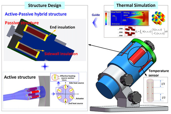
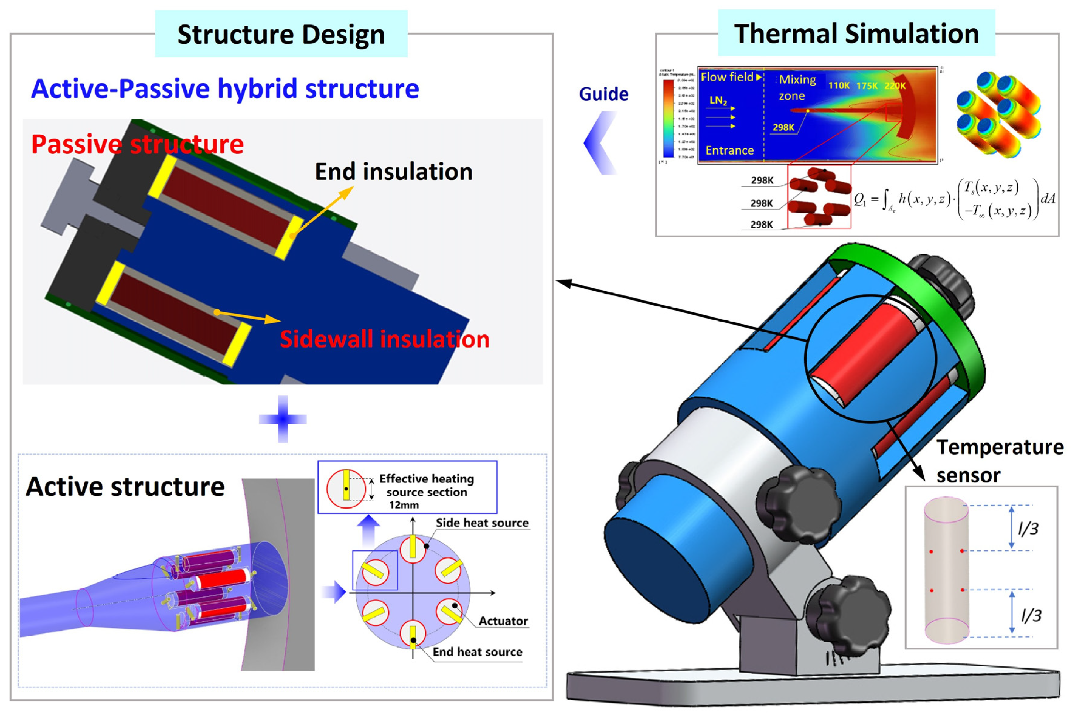
As shown in Figure 1, the proposed temperature control system primarily consisted of a passive thermal insulation structure, a heating source, a temperature acquisition module, and a heat control module. The passive thermal insulation structure employed different materials to cover the various geometric surfaces of the piezoelectric actuator, effectively blocking the majority of the system’s heat dissipation. The addition of the heating source compensated for the limitation of the passive insulation structure in maintaining the system’s temperature level over extended periods while also addressing the temperature uniformity. This was further enhanced by the integration of control algorithms to achieve more precise temperature regulation.

Figure 1. Thermal control system.

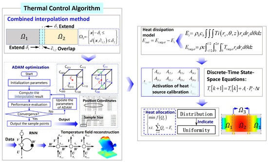
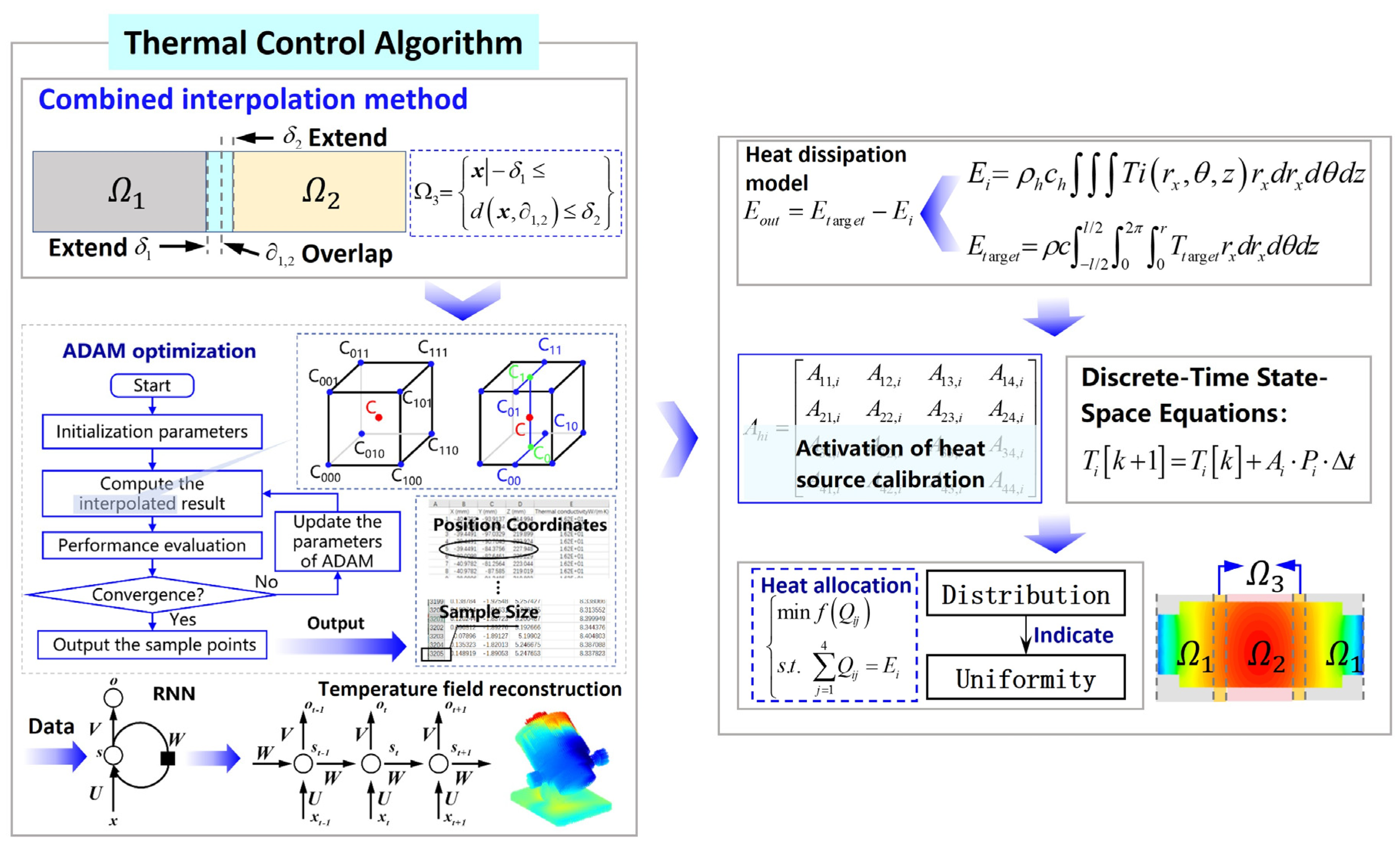
In terms of control, a high-accuracy combined interpolation method for the temperature field was first developed by integrating the simulation data and considering the temperature characteristics of different regions of the system. Based on this, the adaptive moment estimation (ADAM) algorithm was employed to optimize the selection of simulation feature points and balance the accuracy and efficiency of the interpolation process. The optimized simulation dataset, along with the measured data, was used to jointly train a recurrent neural network (RNN) model. This enabled the model to understand the complex relationships between the simulated and measured data and output refined temperature field data. Finally, the combined interpolation method was applied to reconstruct the temperature field. Furthermore, a system heat dissipation model was established. Based on this model, a heat allocation framework was constructed to quantify the heat required for temperature compensation in both global and local regions. Independent heating tests were then conducted for each heat source, and the simulated and measured data were once again integrated. Using an optimization algorithm, the real-time response of individual heat sources to the overall system was obtained, completing the establishment of the entire control algorithm.

3. Active–Passive Hybrid Temperature Control System Design

3.1. Heat Dissipation Analysis

To better understand the thermal behavior of the piezoelectric active vibration suppression system in cryogenic wind tunnel tests, a heat dissipation analysis had to be conducted prior to structural design. It was evident that the primary heat dissipation pathways for the piezoelectric actuators were thermal convection between the sidewalls and the cryogenic air, and the thermal conduction between the actuator ends and the support system. According to Newton’s law of cooling, the heat dissipation power due to thermal convection is given by the following equations [17]:

$$Q_{1 }={\displaystyle {\int }_{A_c} h\left(x,y,z\right)·\left(T_s \left(x,y,z\right)-T_{\infty }\left(x,y,z\right)\right)dA}$$

(1)

$$x\in \left[L_{\mathrm{c}}+t,L_1-L_{\mathrm{p}}-t\right]$$

(2)

where $h(\mathrm{x},\mathrm{y},\mathrm{z})$ is the local convective heat transfer coefficient, $A_c$ is the differential area of the piezoelectric actuator sidewall, $T_s(x,y,z)$ is the local temperature of the sidewall, and $T_{\infty }(x,y,z)$ is the local temperature of the airflow. The heat dissipation power due to thermal conduction and the boundary condition equation of the finite element method is given by the following equation:

$$\left\{\begin{array}{l}{Q}_{2 }={\displaystyle {\int }_{A_e} k·\frac{T_e \left(x,y,z\right)-T_l\left(x,y,z\right)}{L}dA}\\ \nabla ·\left(k(T)\nabla T\right)=0, T\in \mathsf{\Omega }\\ -k{\displaystyle \frac{\mathsf{\partial }T}{\mathsf{\partial }n}}=h\left(x,y,z\right)\left(T-T_{\infty }\right), T\in {\Gamma }_1\\ T=T_{end}, T\in {\Gamma }_2\end{array}\right.$$

(3)

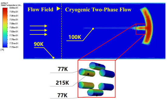
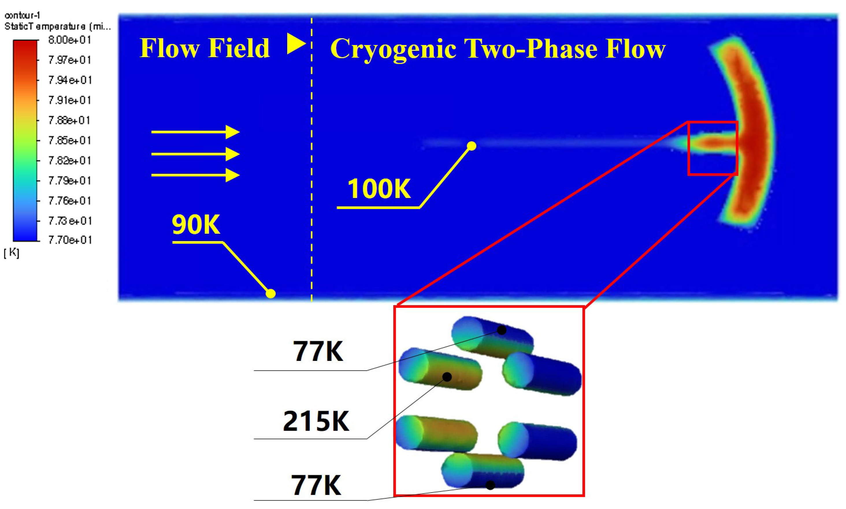
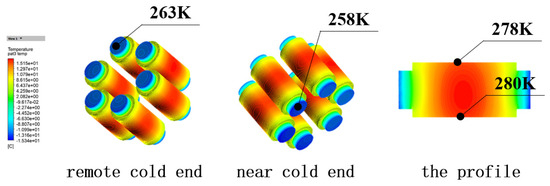
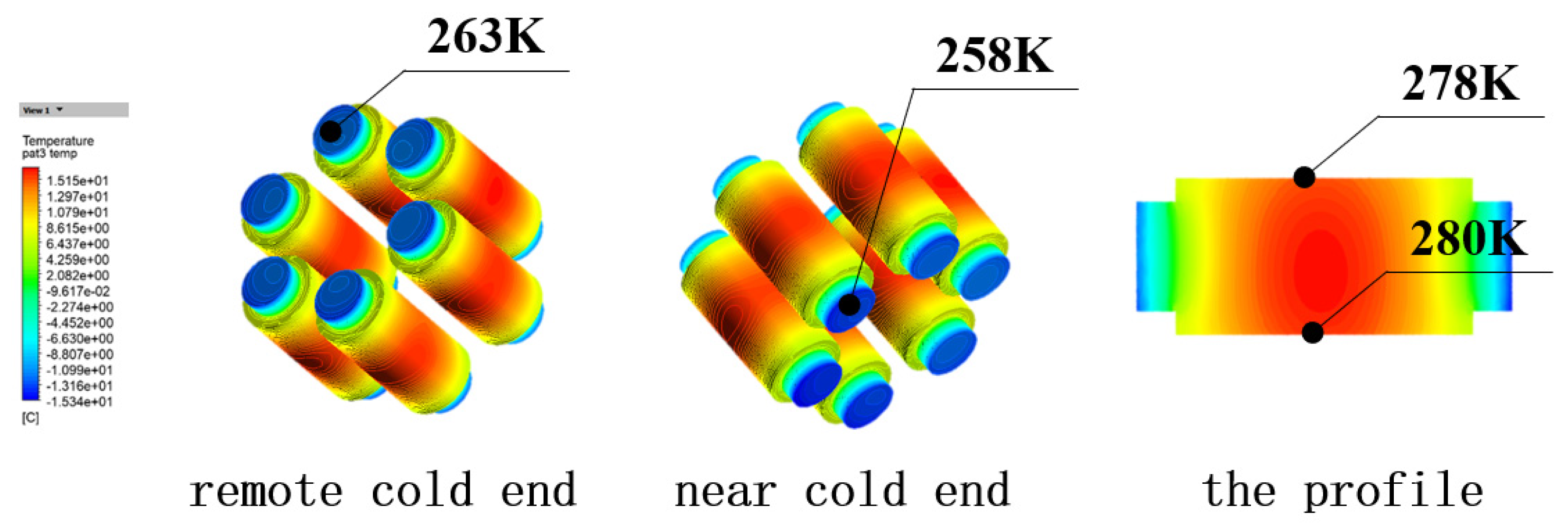
where $\mathrm{k}$ is the thermal conductivity of the material, ${\mathrm{A}}_{\mathrm{e}}$ is the contact area between the end of the piezoelectric actuator and the support rod, $T_e\left(x,y,z\right) - T_l\left(x,y,z\right)$ is the temperature difference between the two, $L$ is the distance from the end to the support system, $k$ is the thermal conductivity, $T_{\infty }$ is the incoming flow temperature, $\mathsf{\Omega }$ is the actuator domain, ${\mathsf{\Gamma }}_1$ is the surfaces exposed to cryogenic flow, and ${\mathsf{\Gamma }}_2$ is the contacting surfaces with the support system. Based on the physical model described above, finite element simulations were conducted under different angle-of-attack conditions. Set the time process to 600 s; the angles of attack to 0°, 10°, and 20°; the wind speeds to 5 m/s, 20 m/s, and 50 m/s; the incoming flow temperature to 90 K, that constitute the boundary condition of the system; the thermal conductivity of zirconia material to 2.5 W/(m·K), that of aerogel material to 0.025 W/(m·K), and that of the piezoelectric actuator to 3 W/(m·K). Given that the incoming flow temperature is extremely low, typically below 90 K, the minor influence of thermal radiation on the system temperature can be considered negligible. The results are shown in Figure 2 and Figure 3. Due to space constraints, Figure 2 is presented only as a schematic illustration of one representative simulation case.

Figure 2. Simulation results for the temperature field under a specific operating condition.

Figure 3. Simulation data analysis.

3.2. Structural Design

Regarding the two heat dissipation paths mentioned in the previous section, the heat loss due to convection was minimized by selecting aerogel as the insulation material for the sidewall to [18] reduce the thermal conductivity of the materials and increase the thickness of the insulation materials. Considering the fact that the actuator end needed to withstand the contact stress, zirconia with high hardness and low thermal conductivity was chosen to block heat conduction [19].

Next, considering the factors that influenced the temperature uniformity, a simulation analysis was conducted on the temperature distribution of the piezoelectric actuator after the incorporation of the thermal insulation structure, as shown in Figure 4. It is evident from the figure that significant axial and radial temperature gradients still existed in the system’s temperature distribution. To address this, a miniature ceramic heating rod was embedded inside the zirconia to serve as an end heat source, with the objective of controlling the axial temperature distribution. Additionally, two flexible PI heating films were selected as side heat sources, covering the upper and lower sides of the actuator. This was primarily intended to regulate the radial temperature distribution. This configuration ultimately formed the heat source distribution illustrated in Figure 1. The two sets of temperature control structures were mutually coupled and closely coordinated, collectively constituting a design scheme for an actively and passively integrated temperature control system.

Figure 4. Temperature distribution of the piezoelectric actuator after the addition of the insulation structure.

4. Hybrid Physical–Virtual Reconstruction Method for Piezoelectric Actuator Temperature Fields

4.1. High-Accuracy Combined Interpolation Method for the Temperature Field

The accurate interpolation of discrete data is crucial for reconstructing temperature fields. However, due to the varying thermal insulation materials used in different locations of a piezoelectric actuator within a passive thermal control structure, a non-uniform temperature distribution exists in the actuator. If the common interpolation methods are applied for temperature field reconstruction, the use of a single interpolation function for global reconstruction may cause temperature gradient discontinuities in the transition zones between the regions of large and small temperature gradients. Moreover, the same interpolation function cannot simultaneously balance the interpolation accuracy for regions with different characteristics.

To solve these problems, this section investigates a local large-gradient temperature interpolation method and a global smooth temperature interpolation method based on temperature gradients across different regions. By combining the transition zones of two regions, a combined interpolation method was formed to prevent abrupt changes in the temperature and its gradient. This framework enabled the real-time precision reconstruction of the system-wide temperature field using discrete point temperature data.

First, quantitative classification was performed on the temperature zones based on different characteristics. Based on linear optimization methods, this study analyzed the thermal distribution across different regions of the piezoelectric actuator. The spatial temperature gradient operator and the temporal temperature gradient operator are defined as

$$G_s\left(i\right)=\left({\displaystyle \frac{\mathsf{\partial }{T}_i}{\mathsf{\partial }x}},{\displaystyle \frac{\mathsf{\partial }{T}_i}{\mathsf{\partial }y}},{\displaystyle \frac{\mathsf{\partial }{T}_i}{\mathsf{\partial }z}}\right)$$

(4)

$$G_t\left(i\right)={\displaystyle \frac{\mathsf{\partial }{T}_i}{\mathsf{\partial }t}}$$

(5)

Based on the spatiotemporal temperature gradient model, the temperature variation characteristics at all nodes within critical system regions under operational conditions were extracted. A nodal significance factor is defined for each node as follows:

$$W_i =\alpha ·G_s\left(i\right) + \beta ·G_t\left(i\right)$$

(6)

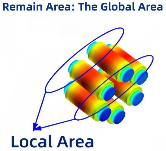
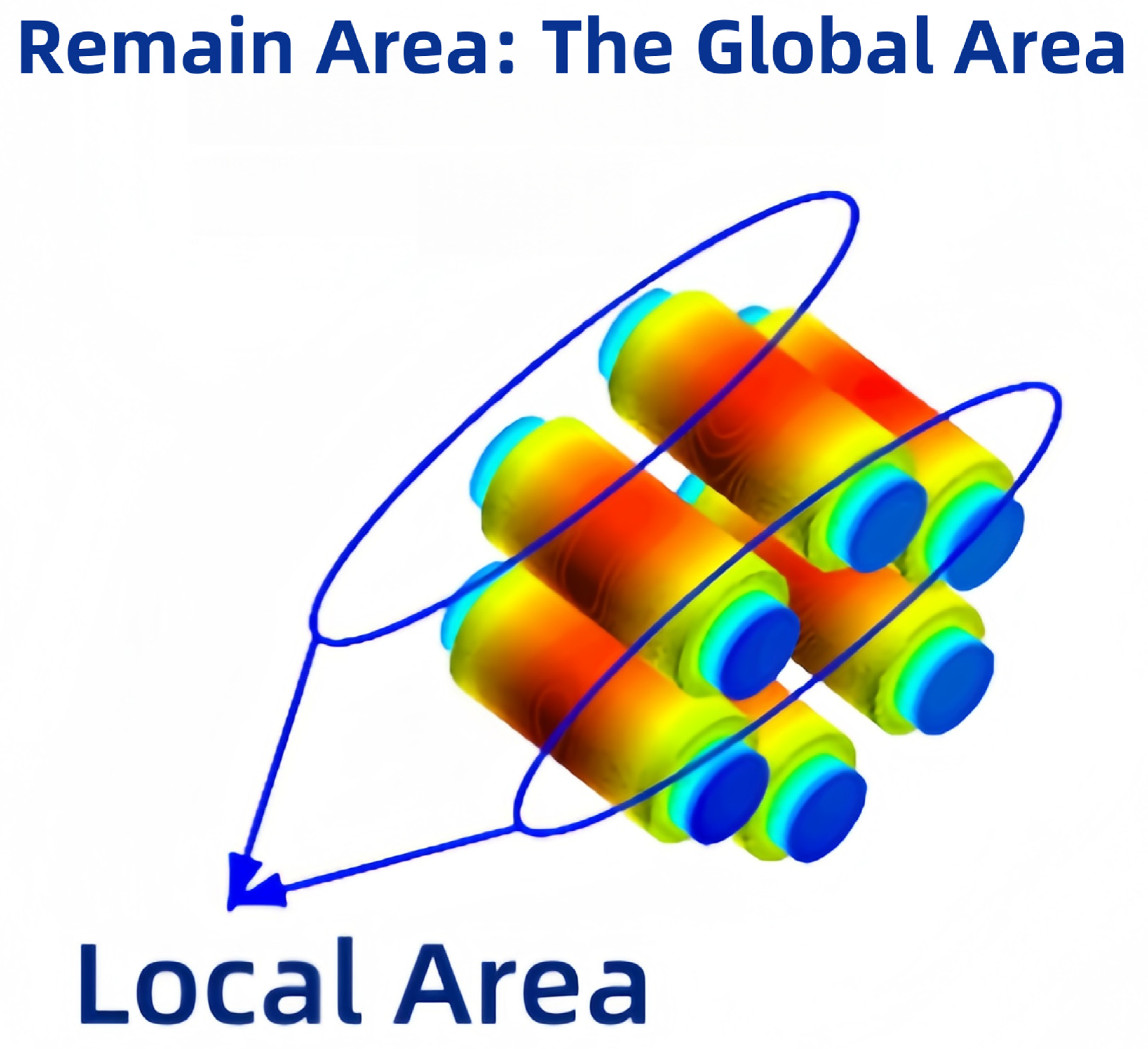
In the expression, α and β denote the weights corresponding to the spatial and temporal temperature gradient operators. Based on Equation (6), importance ranking was performed on all nodes. As depicted in Figure 5, the system was divided into three regions according to the distribution of its temperature gradient: localized region, global region, and transition region. These regions are represented by ${\mathsf{\Omega }}_1$, ${\mathsf{\Omega }}_2$, and ${\mathsf{\Omega }}_3$, respectively. The localized region contained the top 20% of the nodes, while the global region contained the remaining 80%.

Figure 5. Temperature distribution of the piezoelectric actuator after the addition of the insulation structure.

For the localized regions exhibiting high temperature gradients, it is necessary to employ a high-resolution and high-accuracy interpolation method capable of capturing temperature variations at small spatial scales, accordingly, the radial basis function (RBF) interpolation method [19] was adopted. However, the frequently used RBF interpolation, which uses fixed basis functions and parameters and requires empirical parameter adjustments, lacks dynamic adaptability under varying conditions. This limitation compromises model robustness.

To address these limitations, an adaptive RBF interpolation method employing compactly supported basis functions was proposed for achieving high-precision interpolation in high gradient regions. This method is formulated as follows:

$$T\left(\mathbf{c}\right)={\displaystyle \sum _{i=1}^{m_1}{\alpha }_i \varphi \left(\frac{‖\mathbf{c}-{\mathbf{c}}_i‖}{r_i}\right)+{\beta }_0}+{\beta }_{1}x+{\beta }_{2}y+{\beta }_{3}z$$

(7)

$$\varphi \left(r\right)=\begin{array}{cc}\left\{\begin{array}{cc}{\left(1-d\right)}^4\left(4d+1\right),& d\le 1\\ 0,& d>1\end{array}\right. ,& r={\displaystyle \frac{‖\mathbf{c}-{\mathbf{c}}_i‖}{r_i}}\end{array}$$

(8)

In the formula, $T_1\left(\mathit{c}\right)$ represents the local region temperature function, and $\varphi \left(r\right)$ and ${\alpha }_i$ denote the basis function and its corresponding coefficients, respectively. The adaptive support radius $r_i$ can be dynamically adjusted based on specific conditions, as given in the following equation:

$$r_i =min\left({\beta }_v·{\rho }_{m_1},r_{max}\right)$$

(9)

where ${\beta }_v$ is the scaling factor, ${\rho }_{m_1}$ represents the average distance between local simulation particles, and $r_{max}$ denotes the maximum radius value with physical constraints. In this problem, $r_{max}$ is defined from the perspective of heat conduction:

$$r_{max} =\gamma \sqrt{k_h·\Delta t}$$

(10)

where $\gamma$ denotes the regulation coefficient, and $k_h$ represents the thermal conductivity of the local material at the interpolation position. The characteristic time scale $∆t$ is set to the simulation time step resolution.

Based on the characteristic of small temperature gradients across the global region, and given the method’s continuity with respect to distance and high computational efficiency, an inverse distance weighting (IDW) method was employed to establish a smoothed temperature interpolation model [20], which is defined as follows:

$$T_2 (\mathit{x})={\displaystyle \frac{{\displaystyle \sum _{j=1}^{m_2}{w}_j{T}_j}}{{\displaystyle \sum _{j=1}^{m_2}{w}_j}}} ,w_j ={\displaystyle \frac{1}{{‖\mathit{x}-{\mathit{x}}_j‖}^p}} ,\mathit{x}\in {\mathsf{\Omega }}_2$$

(11)

$${\mathbf{x}}_j=\left(x_j,y_j,z_j\right)\left(j=1,2,\dots ,m_2\right)$$

(12)

where $T_2\left(x\right)$ denotes the global region temperature function; $w_j$ represents the weight function, which is used to quantify the magnitude of influence of the temperature at point $x_j$ on the temperature at point $x$; and $p$ denotes the power parameter.

To address the problem of temperature discontinuity easily occurring in the transition regions between the local and global areas, a transition region interpolation method based on weight allocation was developed. This approach achieved a smooth temperature transition and ensured continuity of the temperature field.

First, an overlapping domain was defined at the boundary junction between the two previously studied regions ${\mathsf{\Omega }}_1$ and ${\mathsf{\Omega }}_2$. This overlapping domain was assumed to be the new region formed by the bidirectional elongation of the boundaries of both regions, as shown in the following equation:

$${\mathsf{\Omega }}_3 =\left\{\left.\mathit{x}\right|-{\delta }_1\le d\left(\mathit{x},{\mathsf{\partial }}_{1,2}\right)\le {\delta }_2\right\}$$

(13)

where $d(x,{\mathsf{\partial }}_{1,2})$ denotes the distance from a point in space to the region boundary.

Based on a cosine-type weight function $\eta \left(\mathit{x}\right)$, a smooth transition between the two interpolation schemes is achieved within the overlapping domain:

$$T_3\left(\mathit{x}\right)=\eta \left(\mathit{x}\right)T_1\left(\mathit{x}\right)+\left(1-\eta \left(\mathit{x}\right)\right)T_2\left(\mathit{x}\right),\mathit{x}\in {\mathsf{\Omega }}_3$$

(14)

$$\eta \left(\mathit{x}\right)=\left\{\begin{array}{cc}1& d\left(\mathit{x},{\mathsf{\partial }}_{1,2}\right)\le -{\delta }_1\\ {\displaystyle \frac{1}{2}}\left[1+\cos \left(\pi ·{\displaystyle \frac{d\left(\mathit{x},{\mathsf{\partial }}_{1,2}\right)+{\delta }_1}{{\delta }_1+{\delta }_2}}\right)\right]& -{\delta }_1<d\left(\mathit{x},{\mathsf{\partial }}_{1,2}\right)<{\delta }_2\\ 0& d\left(\mathit{x},{\mathsf{\partial }}_{1,2}\right)\ge {\delta }_2\end{array}\right.$$

(15)

The equation reflects the continuity of temperature within the overlapping domain.

The distinct interpolation methods for the three regions, as described in this section, collectively formed a high-accuracy combined interpolation method for the temperature field. Combined with the data refinement model described in the next section, this enabled the accurate and rapid high-precision reconstruction of the temperature field.

4.2. Construction of the Discrete Data Refinement Model Integrating Simulations and Measurements for the Temperature Field

In the temperature field reconstruction process, more discrete temperature data points led to higher reconstruction accuracy. However, the number of available measurement points is always limited in practical engineering applications. Accordingly, this section describes how the RNN model [21,22] was employed by combining the measured and simulated data to identify the mathematical relationship between them. The goal of this approach was to achieve the real-time prediction of the temperature field based on the measured data, ultimately accomplishing the refinement of the temperature data points.

Before collecting data from actual measurement points, extensive finite element simulations were performed under relevant operating conditions, and the resulting temperature data were compiled into a dataset for training. The operating conditions mainly include four influencing factors: temperatures, inflow velocities, angles of the device, and heat source. All possible combinations of these influencing factors need to be considered to cover all scenarios. To streamline the workload, only a single operating condition is taken into consideration for analysis and calculation in this paper. The sampling of simulation samples introduced the ADAM algorithm [23,24] for optimization. The optimization objective was to ensure that the interpolation results predicted by the final sample points were as close as possible to the real field distribution while maintaining high computational efficiency. The specific form was as follows.

Based on the interpolation method given in the previous section, an interpolation performance evaluation model is defined as follows:

$$P=w_1·A+w_2·S$$

(16)

In the expression, $w_1$ and $w_2$ are undetermined weighting coefficients; $A$ is the reciprocal of the mean squared error between the actual and predicted values of each sample point, which is used to measure model accuracy; and $S$ is the reciprocal of the time interval, which is used to measure the computational speed of the model.

The update rule of ADAM can be expressed as follows:

$$\left\{\begin{array}{l}{v}_t ={\beta }_2 ·v_{t-1 +}\left(1-{\beta }_2\right)·{\left[\nabla P\left({\theta }_{t-1}\right)\right]}^2\\ {\widehat{m}}_t={\displaystyle \frac{m_{t }}{1-{\beta }_1^t}}\\ {\widehat{v}}_t={\displaystyle \frac{v_{t }}{1-{\beta }_2^t}}\\ {\theta }_t={\theta }_{t-1}-\eta ·{\displaystyle \frac{{\widehat{m}}_t}{\sqrt{{\widehat{v}}_t}-\epsilon }}\\ m_{t }={\beta }_1·m_{t-1} +\left(1-{\beta }_1\right)·\nabla P\left({\theta }_{t-1}\right)\end{array}\right.$$

(17)

In the expression, the node location parameter of the simulation samples, denoted as ${\theta }_t$, is a matrix composed of discrete points, with its form defined as follows:

$${\theta }_t=\left[\begin{array}{ccc}{x}_{1t}& y_{1t}& z_{1t}\\ ⋮& ⋮& ⋮\\ x_{mt}& y_{mt}& z_{mt}\end{array}\right]$$

(18)

For the remaining parts, $\nabla P\left({\theta }_{t-1}\right)$ represents the gradient of the interpolation performance function with respect to the node location ${\theta }_{t-1}$, and $m_t$ and $v_t$ are the first-order and second-order moment estimates of the gradient, respectively. ${\beta }_1$ and ${\beta }_2$ are the momentum decay rates, and $\eta$ is the learning rate.

Collect simulation data corresponding to each sample point output by the algorithm and update the dataset. Next, perform cooling experiments under corresponding actual working conditions for all simulation cases, and the characteristics of the measured point data were subsequently collected. Considering the frequent thermal exchange between the high-speed airflow and the actuator in the cryogenic wind tunnel test environment, the system temperature data exhibited periodic variations. This posed certain difficulties in establishing a direct correlation between the measured temperature data and the simulation data. Therefore, to capture the dynamic characteristics of the temperature data at the measured points, data processing was performed in both the time and frequency domains. For the time point $t_i$, the time-domain feature matrix at any measurement point is shown in the following equation:

$$F_T=\left[T\left(t_i\right),{\displaystyle \frac{dT}{dt}}\left(t_i\right),{\displaystyle \frac{d^{2}T}{d{t}^2}}\left(t_i\right)\right]$$

(19)

Performing fast Fourier transform (FFT) on this matrix yields the frequency domain feature matrix:

$$X\left(k\right)=FFT\left(T\left(t\right)\right)$$

(20)

For the generated frequency domain signal $X\left(k\right)$, the dominant frequency components are extracted. These dominant frequency components are combined with their corresponding amplitudes to form the frequency domain feature matrix:

$$F_F=\left[f_i,A_i\right]$$

(21)

In the equation, $f_i$ and $A_i$ are the dominant frequency and the amplitude value at moment $t_i$, respectively.

After obtaining the time–frequency feature matrix from the measured data, the matrix is used as the input matrix to construct the RNN model, which consists of one input layer, one hidden recurrent layer, and one output layer. The hidden layer comprises 128 memory units, each implemented using the simple RNN cell. The choice of a single hidden layer with 128 units balances model capacity and computational efficiency for real-time temperature field reconstruction. The dataset was randomly split into training (60%), validation (20%), and test (20%) sets. The ADAM optimizer is used to update the network weights and the mean squared error between the predicted and the true temperature fields is adopted as the loss function. Finally, to prevent overfitting, the Dropout regularization strategy is adopted. The model is shown in the following equations:

$$\left\{\begin{array}{l}{h}_t={\sigma }_p(W_{in}{x}_t +W_h{h}_{t-1}+b_h)\\ \\ y_t=softmax(W_{out}{h}_t+b_{out})\\ \\ L={\displaystyle \frac{1}{B}}{\displaystyle \sum _{b=1}^B\frac{1}{M}{\displaystyle \sum _{m=1}^M‖{\widehat{T}}_m^{(b)}-T_m^{(b)}‖}}\end{array}\right.$$

(22)

$$x_t=\left[F_T,F_F\right]$$

(23)

where $t$ is the time step, $x_t$ is the input vector, $h_t$ is the hidden state vector, and $y_t$ is the output vector. $W_{in}$ is the input weight matrix, $W_h$ is the hidden state weight matrix, and $W_{out}$ is the output weight matrix. $b_h$ is the bias vector for the hidden layer, and $b_{out}$ is the bias vector for the output layer. $L$ is the loss function, $B$ is the batch size and $M$ is the sequence length. The activation function that is employed is the hyperbolic tangent function, which is defined as ${\sigma }_p=tanh$.

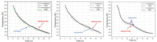
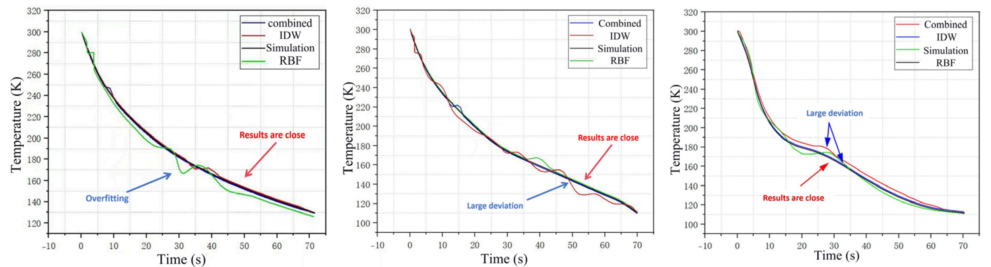
After training was completed, the full-field temperature data could be predicted using discrete measurement points, thereby enabling the reconstruction of the temperature field based on the interpolation method proposed in the previous section. Finally, three representative locations were selected to compare the temperature field reconstruction results with those that were obtained using single interpolation methods. The error analysis was conducted based on the results of the simulation calculations, as shown in Figure 6.

Figure 6. Comparison of interpolation results of verification points.

It can be seen from the figure that the temperature field reconstruction method proposed in this section demonstrated excellent fitting performance at different locations, and the error remained within acceptable limits, which validated the effectiveness of the method.

5. Multi-Heat Source Collaborative Adaptive Control Method

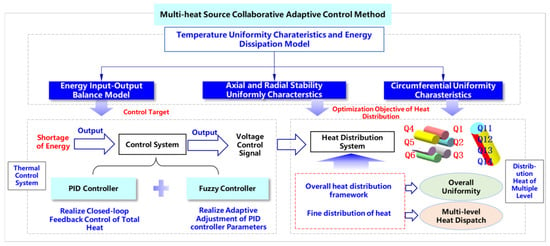
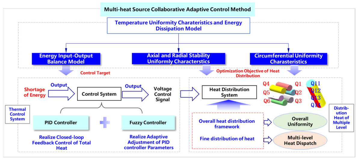
The framework of the multi-heat source collaborative adaptive control method proposed in this section is illustrated in Figure 7. First, using the full-field temperature data provided by the temperature field reconstruction, an energy dissipation model was established, and the temperature uniformity indices were quantified. Subsequently, the control program was divided into two components: an overall thermal control module and a thermal allocation module. The overall thermal control module tracked the real-time full-field temperature data and adjusted the overall thermal output to replenish the system’s thermal deficit. The thermal allocation module captured the thermal uniformity status of the system and distributed the total heat among the individual heat sources. Ultimately, this achieved adaptive thermal regulation for the system.

Figure 7. Adaptive control principle based on temperature uniformity.

5.1. Thermal Dissipation Model Based on Full-Field Temperature Sensing

The objective of overall thermal management is to ensure dynamic equilibrium between a system’s thermal consumption and input. Consequently, the establishment of an efficient and accurate model for system thermal dissipation is paramount. Traditional thermal dissipation models are predominantly reliant on classical thermo-dynamics theory. This approach suffers from slow computational speeds, rendering it unsuitable for the real-time control of thermal management systems. Therefore, the primary goal of this section is to propose a thermal dissipation model that balances computational efficiency and accuracy. This model will lay the groundwork for the construction of an overall thermal management framework.

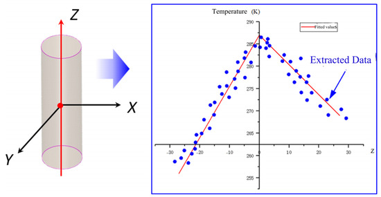
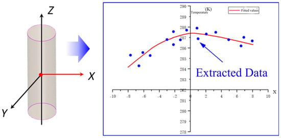
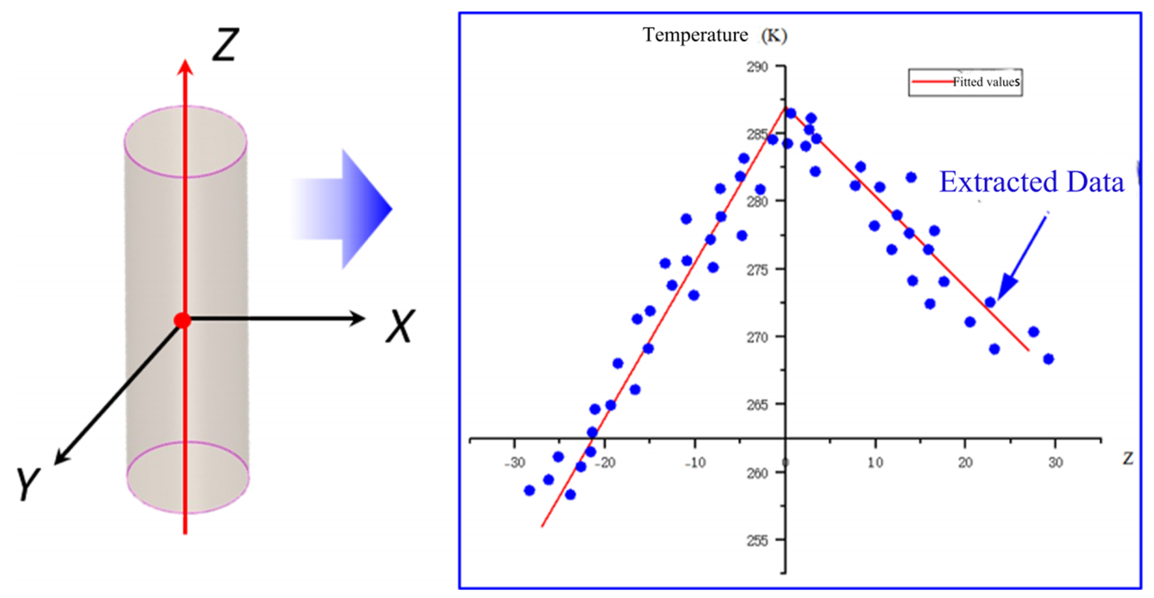
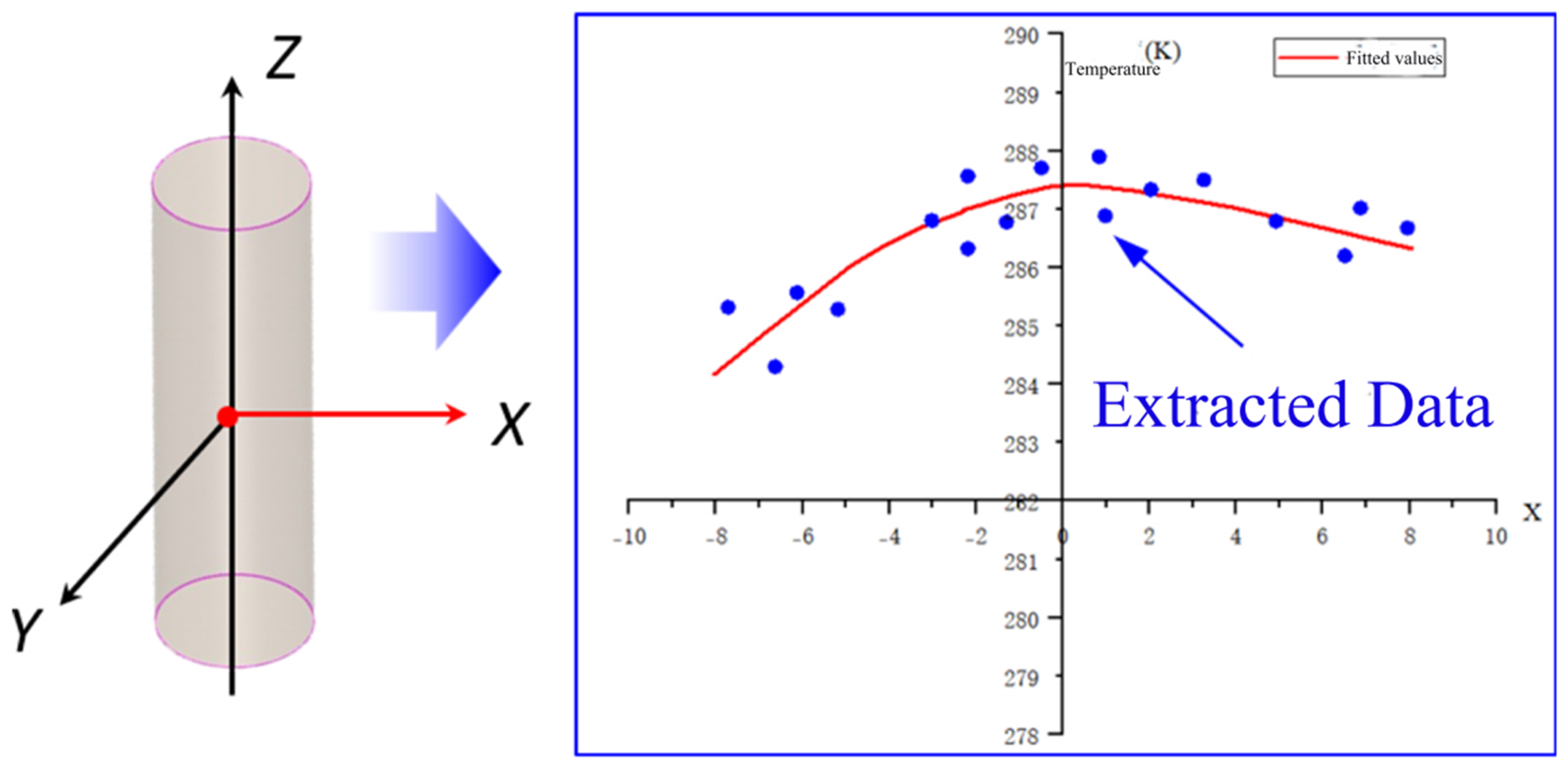
Based on the temperature field reconstruction results presented in Section 4, the temperature data along the actuator axis and across the diameter of the midsection cross plane at identical time points were extracted, as illustrated in Figure 8. Using the full-field temperature sensing data as input, the temperature profiles were fitted with the following outcomes.

$$T_{c,i} (z)=\left\{\begin{array}{cc}{T}_{c,i}-{\displaystyle \frac{z}{l/2}}\left(T_{c,i}-T_{1,i}\right)& z\in \left[-{\displaystyle \frac{l}{2}},0\right]\\ T_{c,i}+{\displaystyle \frac{z}{l/2}}\left(T_{c,i}-T_{2,i}\right)& z\in \left[0,{\displaystyle \frac{l}{2}}\right]\end{array}\right.$$

(24)

$$T_i\left(r_x,\theta ,z\right)=\left\{\begin{array}{cc}{T}_{c,i} (z)-\left(T_{c,i} (z)-T_{3,i} \right){\left({\displaystyle \frac{r_x}{r}}\right)}^2,& \theta \in \left[0,\pi \right]\\ T_{c,i} (z)-\left(T_{c,i} (z)-T_{4,i} \right){\left({\displaystyle \frac{r_x}{r}}\right)}^2,& \theta \in \left[\pi ,2\pi \right]\end{array}\right.$$

(25)

Equations (24) and (25) correspond to the axial and radial temperature functions, respectively.

Figure 8. Temperature variation along different directions of the piezoelectric actuator.

For the $i$-th actuator, the thermal energy calculation is expressed as follows:

$$E_i ={\rho }_h{c}_h{\displaystyle {\int }_{-l/2}^{l/2}{\displaystyle {\int }_0^{2\pi }{\displaystyle {\int }_0^r{T}_i\left(r_x,\theta ,z\right)}}}{r}_{x}d{r}_{x}d\theta dz$$

(26)

In the expression, ${\rho }_h$ and $c$ represent the density of the actuator and its specific heat capacity, respectively. The thermal energy corresponding to the target temperature field is expressed as follows:

Equations (24) and (25) correspond to the axial and radial temperature functions, respectively.

$$E_{t\arg et} =\rho c{\displaystyle {\int }_{-l/2}^{l/2}{\displaystyle {\int }_0^{2\pi }{\displaystyle {\int }_0^r{T}_{t\arg et}}}}{r}_{x}d{r}_{x}d\theta dz$$

(27)

Therefore, the energy dissipation model can be expressed as follows:

$$E_{out}={\displaystyle \sum _{i=1}^6{E}_{t\arg et}-E_i}$$

(28)

The proposed model was used to evaluate the total thermal dissipation during the dynamic temperature variations in the computational system discussed in Section 4. The model transformed the complex problem of temperature field tracking into a thermal compensation issue, providing a quantitative foundation for the subsequent design of control methods.

5.2. Overall Thermal Control Framework Based on Fuzzy Adaptive PID

The primary control objective of the system was to ensure that the input energy consistently matched the dissipated energy, thereby maintaining the controlled system in a desired stable thermal state. To achieve this objective, a closed-loop PID control strategy was employed. The PID controller’s time-domain expression is given as follows:

$$u(t)=K_{P}e(t)+K_i{\displaystyle \int e(t)dt}+K_d{\displaystyle \frac{de(t)}{dt}}$$

(29)

where $u\left(t\right)$ denotes the output signal, and $e\left(t\right)$ represents the error signal.

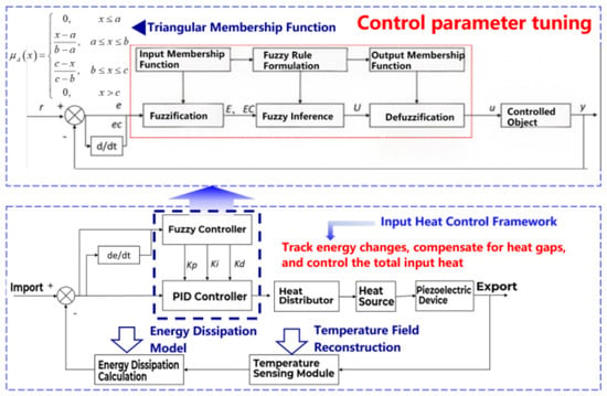
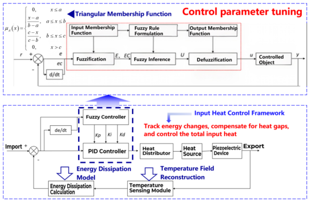
Due to real-time fluctuations in temperature parameters during physical experiments, the parameters of a PID controller must possess adaptive adjustment capabilities. To achieve this, a fuzzy controller was introduced for tuning. The input variables for the fuzzy controller were defined as the error $e$ between the actual heat and the target heat calculated based on the energy dissipation model, along with the error change rate $de$. The output variables were the PID controller parameters $K_p$, $K_i$, and $K_d$. The resulting fuzzy adaptive PID control framework is illustrated in Figure 9.

Figure 9. Schematic of the fuzzy PID control framework.

In this work, a triangular membership function was employed to describe fuzzy sets, with the specific form given as follows:

$${\mu }_A\left(x\right)=\left\{\begin{array}{cc}0,& x\le a\\ {\displaystyle \frac{x-a}{b-a}},& a\le x\le b\\ {\displaystyle \frac{c-x}{c-b}},& b\le x\le c\\ 0,& x>c\end{array}\right.$$

(30)

Then, the process of fuzzy inference was expressed using IF-THEN rules, as shown in the following equation:

$$\mathrm{If} \mathrm{E} \mathrm{is} \mathrm{NB} \mathrm{and} \mathrm{EC} \mathrm{is} \mathrm{NB}, \mathrm{then} K_p \mathrm{is} \mathrm{IAD}, K_i \mathrm{is} \mathrm{ISL}, K_d \mathrm{is} \mathrm{ISL}$$

(31)

The fuzzy rules that correspond to the proportional gain $K_p$, integral gain $K_i$, and derivative gain $K_d$ are shown in Table 1, Table 2 and Table 3, respectively.

Table 1. Fuzzy rules corresponding to the proportional gain $K_p$.

EC E	NB	NS	ZO	PS	PB
NB	IAD	ISL	K	RSL	RAD
NS	ISL	K	RSL	RAD	RAD
ZO	K	RSL	K	ISL	IAD
PS	RSL	RAD	ISL	K	ISL
PB	RAD	RAD	IAD	ISL	K

Table 2. Fuzzy rules corresponding to the integral gain $K_i$.

EC E	NB	NS	ZO	PS	PB
NB	ISL	K	RSL	RAD	RAD
NS	K	RSL	RAD	RAD	RSL
ZO	RSL	RAD	K	ISL	ISL
PS	RAD	RAD	ISL	K	K
PB	RAD	RSL	ISL	K	RSL

Table 3. Fuzzy rule corresponding to the differential gain $K_d$.

EC E	NB	NS	ZO	PS	PB
NB	ISL	K	RSL	RAD	RAD
NS	K	RSL	RAD	RAD	RSL
ZO	RSL	RAD	K	ISL	ISL
PS	RAD	RAD	ISL	K	K
PB	RAD	RSL	ISL	K	RSL

In this framework, the input to the control system was the error between the calculated energy of the piezoelectric device and the target energy. This input was processed by a fuzzy adaptive PID controller, which output a control signal to adjust the heat input $E_{in}$ to the system. The output signal then served as the input to the thermal allocation module. After processing with this module, the system’s temperature distribution was influenced. The altered system temperature was computed using the temperature field reconstruction module and the energy dissipation model, updating the system state. This updated state was fed back into the system, and the control parameters were continuously adjusted based on real-time system conditions until the desired control objectives were achieved, thereby achieving closed-loop feedback control.

5.3. Development of an Experimental–Simulation Integrated Multi-System Thermal Allocation Module

Based on the analysis in the preceding section, it was determined that the total energy input required for the piezoelectric actuator varied across different temperature states. The core issue discussed in this section is the determination of how to rationally distribute the total energy among individual systems to achieve uniformity in the temperature field allocation. Before the thermal allocation module could be constructed, a quantitative model for reaction temperature uniformity had to be established.

For piezoelectric actuators, multiple circumferentially arranged actuators collectively form an overall thermal system in three-dimensional space, while each actuator individually constitutes several sub-systems. Temperature uniformity is primarily manifested as uneven heat distribution among axial sub-systems at the overall system scale, and as axial and radial temperature gradients within individual actuators at the sub-system scale. Thus, the temperature uniformity can be quantified by calculating the standard deviations of temperature along three distinct dimensions and directions. Based on the temperature field reconstruction model established in Section 4, the system’s temperature field function $\mathrm{T}\left(x,y,z,t\right)$ can be readily obtained, enabling the straightforward derivation of the average temperature for piezoelectric actuators:

$$T_{avg,i}={\displaystyle \frac{{\displaystyle {\int }_{V}T\left(x,y,z,t\right)dV}}{V}},i=1,2\cdots 6$$

(32)

where $V$ is the volume of the piezoelectric actuator.

The circumferential temperature uniformity indicator for the overall system is denoted as

$${\sigma }_{\mathrm{circle}}=\sqrt{{\displaystyle \frac{1}{6}}{\displaystyle \sum _{i=1}^6{\left(T_{avg,i}-{\overline{T}}_{avg}\right)}^2}}$$

(33)

For the sub-system that is composed of a single piezoelectric actuator, the axial temperature uniformity indicator is given in the following equation:

$${\sigma }_{\mathrm{axial},\mathrm{i}}=\sqrt{{\displaystyle \frac{1}{2}}\left({\left(T_{c,i}-T_{1,i}\right)}^2+{\left(T_{c,i}-T_{2,i}\right)}^2\right)}$$

(34)

The radial temperature uniformity indicator is denoted as

$${\sigma }_{\mathrm{radial},\mathrm{i}}=\sqrt{{\displaystyle \frac{1}{2}}\left({\left(T_{c,i}-T_{3,i}\right)}^2+{\left(T_{c,i}-T_{4,i}\right)}^2\right)}$$

(35)

The temperature uniformity indicator for the sub-system is formulated by combining the aforementioned indicators with the corresponding coefficients A and B, as expressed in following equation:

$${\sigma }_{\sin \mathrm{gle},\mathrm{i}}=A·{\sigma }_{\mathrm{axial},\mathrm{i}}+B·{\sigma }_{\mathrm{radial},\mathrm{i}}$$

(36)

Based on the previous analysis, the first step involves completing the circumferential thermal allocation for the overall system, which can easily be done.

• For the $i$-th actuator, the weight coefficient of the thermal is defined as follows:

$$W_{heat,i}={\displaystyle \frac{\frac{1}{T_{avg,i}}}{{\displaystyle \sum _{i=1}^6\frac{1}{T_{avg,i}}}}}$$

(37)

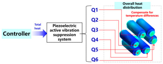
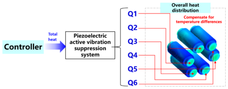
• Then, the respective energy input $E_{in,i}$ for each actuator is

$$E_{in,i} =W_{heat,i} \times E_{in}$$

(38)

The thermal allocation framework for the integrated system is represented in Figure 10.

Figure 10. Overall heat distribution framework of the system.

After the completion of the heat distribution for the overall system, the amount of available heat in each sub-system could be quantitatively calculated. The various types of heat sources deployed in a sub-system had different contributions to each point in the temperature field, and it was difficult to establish an accurate physical model for characterization. It was also difficult to accurately elucidate these quantitative relationships using conventional analytical modeling techniques. However, based on the experience discussed in Section 4, an experimental–simulation integrated optimization approach could still be developed to establish an accurate function in real time to describe the relationship between the heat source inputs and the characteristic point temperature responses.

Based on the principle of temperature field superposition and the reconstruction results detailed in Section 4, each heat source on the target actuator was individually activated, and the temperature field point data were collected at each time instant. Taking the $i$-th actuator as an example, the discrete-time state-space equations were constructed to obtain the specific form of the coefficient matrices.

$$T_i\left[k+1\right]=T_i\left[k\right]+A_i·P_i·\Delta t$$

(39)

$$A_i=\left[\begin{array}{cccc}{A}_{11,i}& A_{12,i}& A_{13,i}& A_{14,i}\\ A_{21,i}& A_{22,i}& A_{23,i}& A_{24,i}\\ A_{31,i}& A_{32,i}& A_{33,i}& A_{34,i}\\ A_{41,i}& A_{42,i}& A_{43,i}& A_{44,i}\end{array}\right]$$

(40)

$$P_i={\left[\begin{array}{cccc}{P}_{i1}& P_{i2}& P_{i3}& P_{i4}\end{array}\right]}^T$$

(41)

where $A_i$ is the coefficient matrix of the power-temperature change rate.

For the $j$-th heat source, the relationship between its power $P_{ij}$ and heat output $Q_{ij}$ can be expressed as follows:

$$\left\{\begin{array}{l}{Q}_{ij}=P_{ij}·\Delta t,j=1,2,3,4\\ {\displaystyle \sum _{j=1}^4{Q}_{ij}}=E_{in,i}\end{array}\right.$$

(42)

By solving the above five equations simultaneously, an exact temperature response function for the heat-source/input-characteristic-point can be obtained. This enables the temperature at the characteristic points on the actuator to be indirectly represented by the heat output $Q_{ij}$ of the heat source. Consequently, the temperature uniformity index introduced in the previous section can be reformulated as a temperature-heat source function, with the specific form shown below:

$${\sigma }_{\mathrm{axial},\mathrm{i}}\left(Q_{\mathrm{ij}}\right)=\sqrt{{\displaystyle \frac{1}{2}}\left({\left(T_{c,i}\left(Q_{\mathrm{ij}}\right)-T_{1,i}\left(Q_{\mathrm{ij}}\right)\right)}^2+{\left(T_{c,i}\left(Q_{\mathrm{ij}}\right)-T_{2,i}\left(Q_{\mathrm{ij}}\right)\right)}^2\right)}$$

(43)

$${\sigma }_{\mathrm{radial},\mathrm{i}}\left(Q_{\mathrm{ij}}\right)=\sqrt{{\displaystyle \frac{1}{2}}\left({\left(T_{c,i}\left(Q_{\mathrm{ij}}\right)-T_{3,i}\left(Q_{\mathrm{ij}}\right)\right)}^2+{\left(T_{c,i}\left(Q_{\mathrm{ij}}\right)-T_{4,i}\left(Q_{\mathrm{ij}}\right)\right)}^2\right)}$$

(44)

$$f\left(Q_{ij}\right)=A·{\sigma }_{\mathrm{axial},\mathrm{i}}\left(Q_{\mathrm{ij}}\right)+B·{\sigma }_{\mathrm{radial},\mathrm{i}}\left(Q_{\mathrm{ij}}\right)$$

(45)

Thus, an optimization problem intended to achieve maximum temperature uniformity for individual units is constructed, as formulated in the following equation:

$$\left\{\begin{array}{l}\begin{array}{ccc}s.t.& {\displaystyle \sum _{j=1}^4{Q}_{ij}}=E_{in,i}& Q_{ij}\ge 0\end{array} \\ \min f\left(Q_{ij}\right)\end{array}\right.$$

(46)

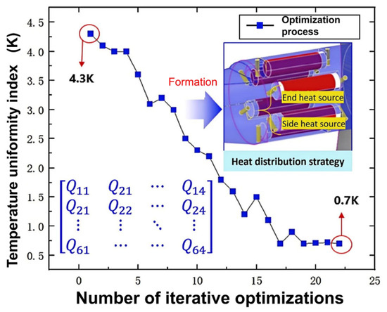
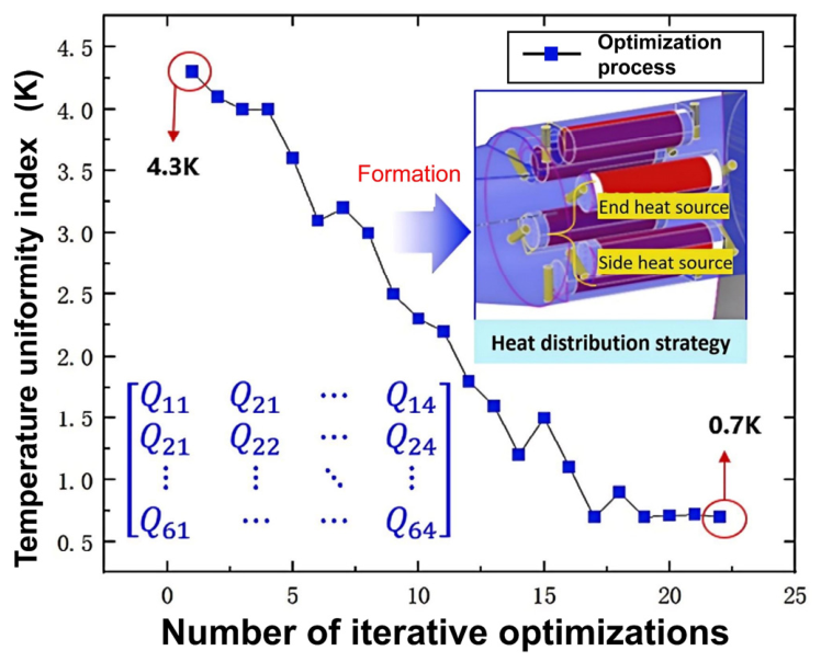
Taking the temperature distribution obtained after 30 s of cooling at 77 K and a 20° angle of attack as the simulation case, the optimization progress under these conditions was plotted, as shown in Figure 11. Upon final convergence, the corresponding thermal allocation for each heat source was determined.

Figure 11. Optimization process of refined heat distribution from each heat source.

This completed the design of the thermal allocation methodology for all heat sources, achieving high efficiency utilization of the total thermal energy delivered to the piezoelectric device while maintaining uniform temperature distribution across the system.

6. Experiment

6.1. Experimental Setup

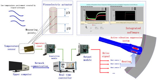
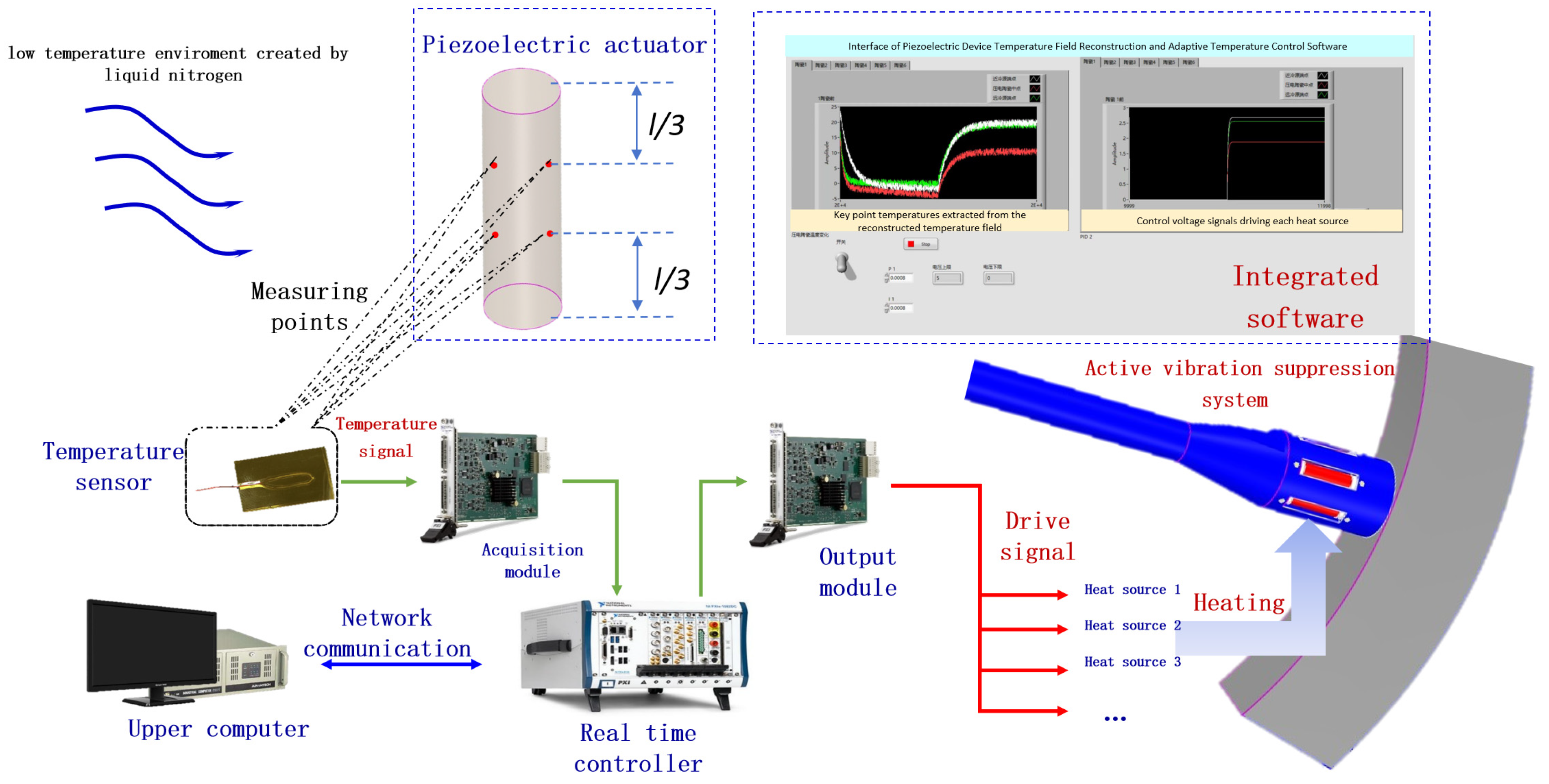
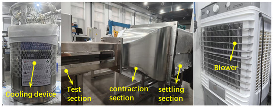
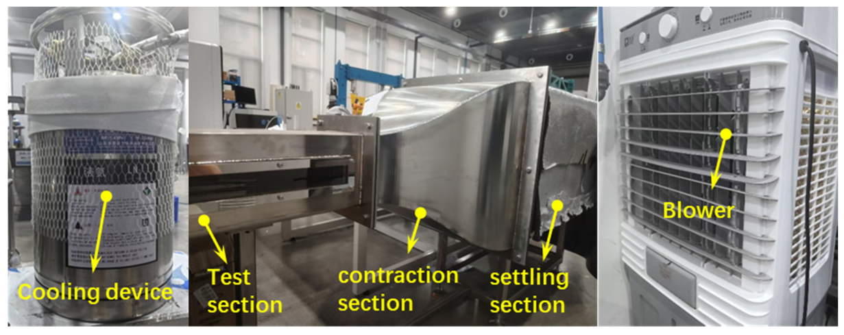
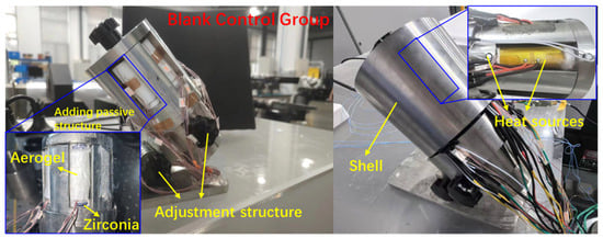
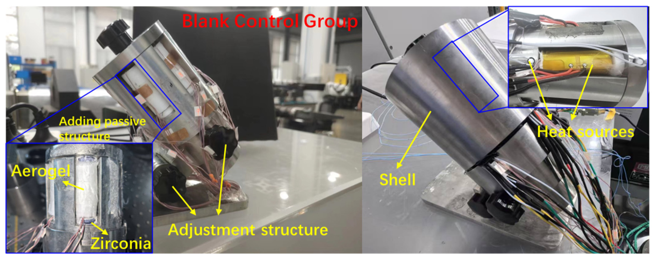
Based on the thermal control structure and control method proposed in the preceding sections of this paper, a heat preservation performance test platform was established, as illustrated in Figure 12. This platform consisted of a small-scale cryogenic wind tunnel, a piezoelectric vibration suppression system, and a measurement and control hardware. The wind tunnel consisted of a cooling device, blower, test section, contraction section, and settling section, as illustrated in Figure 13. To achieve a low-temperature flow field environment, liquid nitrogen was used as the coolant medium, resulting in a flow temperature of 77 K and a velocity of 6.9 m/s. For the piezoelectric vibration suppression system, the experiment primarily targeted the six circumferentially distributed piezoelectric actuators, as illustrated in Figure 14. The entire hardware system included a Type T thermocouple, a controller, a host computer, and a temperature acquisition board. Six thermocouples for the temperature measurement on each actuator were grouped in sets of three. Each set was uniformly spaced circumferentially at a location that was one-third of the length from each end to facilitate the real-time reconstruction of the temperature field and collect data at targeted locations of interest. Before the experiment begins, it is necessary to perform both static and dynamic calibration on all thermocouple sensors to ensure their static and dynamic measurement accuracy. The static calibration is carried out by measuring the same flat plate at room temperature using pre-calibrated equipment. Dynamic calibration is conducted on a heating stage, where data from the device to be calibrated and a standard device are recorded during the heating process, and characteristics such as the response time of both are compared. The sampling frequency for all measurements is set to 20 Hz. The relevant software was developed on the LABVIEW platform (v2015). Furthermore, the proposed method was verified by ground experiments.

Figure 12. Experimental setup.

Figure 13. Small-scale cryogenic wind tunnel.

Figure 14. Thermal control structure.

The purpose of this experiment was to evaluate whether the proposed thermal control method could maintain temperature uniformity in piezoelectric actuators while ensuring effective thermal insulation under cryogenic conditions. Therefore, an experimental setup was configured without the passive thermal control structure and active thermal control, retaining only the original piezoelectric active vibration suppression system and temperature measurement points. This configuration exposed sensitive components directly to the cryogenic flow field cooled by liquid nitrogen. Temperature data were collected to assess relevant performance metrics, establishing this configuration as the blank control group.

The piezoelectric active vibration suppression system that was added to the thermal control structure was taken as the research object. For a single experimental run of this system, the protocol was divided into two phases based on the activation status of the active thermal control system:

In Phase 1 of the experiment (starting with the injection of liquid nitrogen and lasting for 300 s), active thermal control remained deactivated, allowing only the passive thermal control structure to impede heat dissipation. Then, the experiment proceeded to Phase 2 (lasting for 1500 s), active thermal control was activated immediately upon completion of Phase 1 and maintained until the experiment concluded, enabling simultaneous operation of both passive and active thermal control systems.

Following the experiment, temperature uniformity indicators proposed in Section 5 were calculated separately for both phases. Phase 1 of the experiment, along with the control group, formed a controlled experiment to evaluate the effectiveness of the passive thermal insulation structure. Additionally, Phases 1 and 2 constituted a self-controlled experiment that was used to assess the effectiveness of the method after the intervention of active control.

6.2. Analysis of Experimental Results

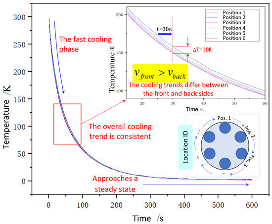
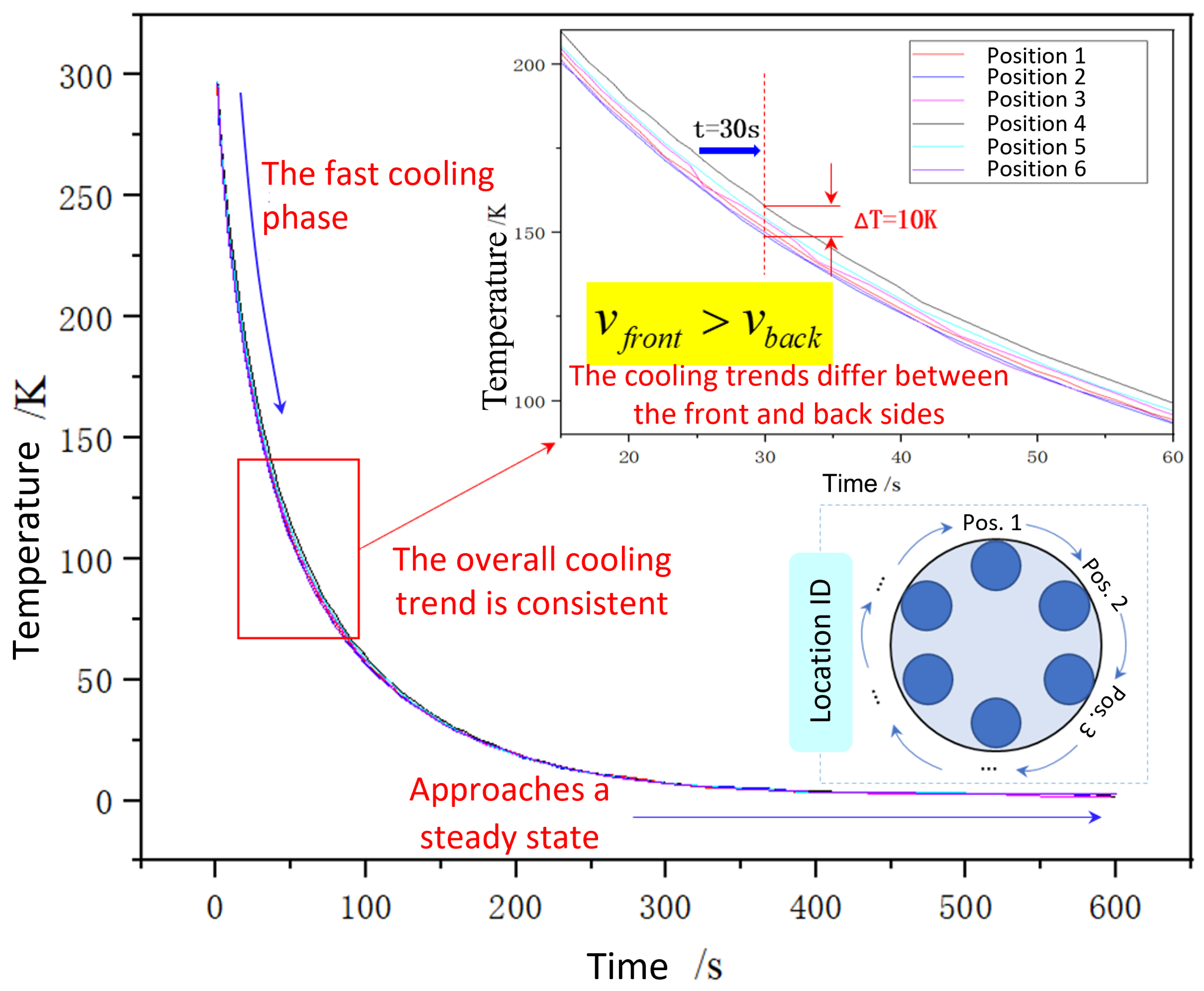
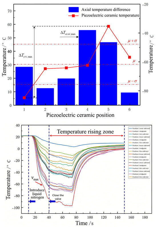
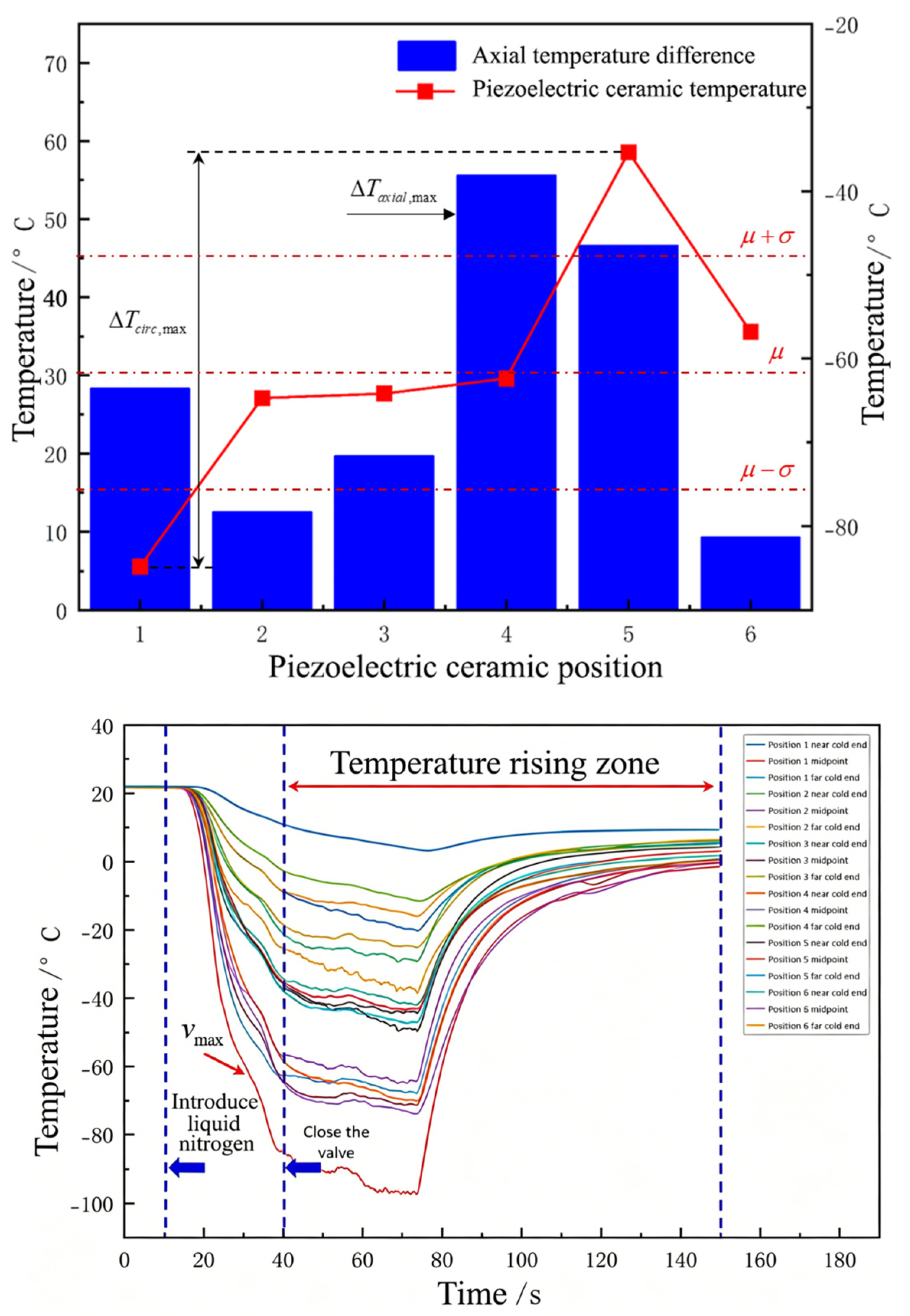
The experimental data for the blank control group are presented in Figure 15 and Table 4. As indicated in the figure and table, the prototype system without any thermal control structures exhibited a rapid temperature decline in the liquid nitrogen cryogenic environment, with the maximum cooling rate among all key measurement points exceeding 255 K/min. To prevent the equipment from becoming too cold, we conveyed liquid nitrogen for only 30 s. Additionally, the temperature exhibited significant variations in all directions. The axial, circumferential, and radial maximum temperature differences in the system exceeded 55 K, 49 K, and 13 K, respectively. Additionally, according to the temperature uniformity indicators presented in Section 5, the actuator exhibited marked temperature variations across all directions. Figure 16 presents the temperature variations in all six piezoelectric actuators in the experimental group, while Table 5 and Table 6 detail the calculated temperature assessment indicators for the two experimental phases.

Figure 15. Experimental data for the blank control group.

Table 4. Temperature assessment indicators of the blank control group.

Indicator	Value
Average cooling rate (K/min)	138.2
Maximum cooling rate (K/min)	255.7
Axial uniformity indicator (K)	32.9
Axial temperature range (K)	155.6
Radial uniformity indicator (K)	8.4
Radial temperature range (K)	13.7
Circumferential uniformity indicator (K)	14.5
Circumferential temperature range (K)	49.5

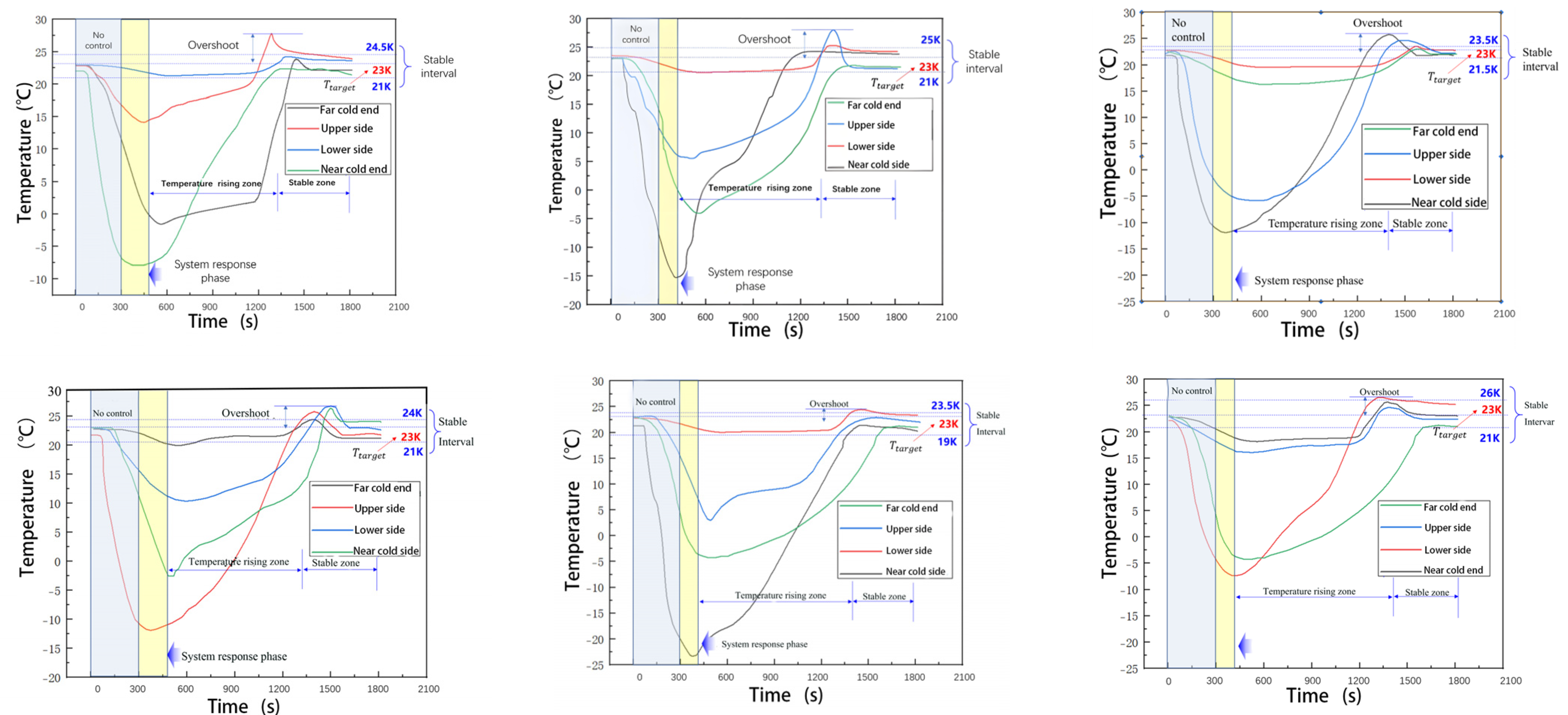
Figure 16. Process of temperature variation at the key points of the piezoelectric element over time.

Table 5. Temperature assessment indicators for Phase 1.

Indicator	Value
Average cooling rate (K/min)	2.4
Maximum cooling rate (K/min)	5.7
Axial uniformity indicator (K)	5.2
Axial temperature range (K)	19.1
Radial uniformity indicator (K)	6.5
Radial temperature range (K)	17.1
Circumferential uniformity indicator (K)	2.6
Circumferential temperature range (K)	7.6

Table 6. Temperature assessment indicators for Phase 2.

Indicator	Value
Average temperature control deviation (K)	0.9
Maximum temperature control deviation (K)	1.2
Axial uniformity indicator (K)	2.1
Axial temperature range (K)	2.3
Radial uniformity indicator (K)	1.5
Radial temperature range (K)	3
Circumferential uniformity indicator (K)	0.15
Circumferential temperature range (K)	0.9

The results showed that following the activation of the active control system, the temperatures for all of the piezoelectric elements continued to exhibit a gradual decline for a brief period due to thermal response lag. Furthermore, the temperatures at certain locations exceeded the set point temperature during the subsequent heating process, indicating the presence of an overshoot phenomenon.

A comparative analysis of the temperature assessment indicators between the control group and the Phase I experimental group revealed that after the addition of the passive thermal control structure, the actuator achieved significantly lower cooling rates under cryogenic conditions. The maximum cooling rate across all calculated points was below 6 K/min, and the average cooling rate was below 3 K/min. Compared with the control group, this represented a 98% enhancement in the thermal insulation performance, which confirmed the effectiveness of the passive thermal control structure. In addition, the thermal uniformity was enhanced at the same time. However, experimental results simultaneously indicated that a significant temperature gradient persisted, and the system continued to exhibit slow cooling in the cryogenic environment even after incorporating the passive thermal control structure. Without external intervention, this configuration remained insufficient to meet the testing requirements of cryogenic wind tunnel experiments (which may extend to several hours). Consequently, relying solely on passive thermal control structures for thermal insulation cannot achieve persistent and stable thermal management for piezoelectric devices. To achieve further optimization, active thermal control needed to be implemented.

Furthermore, by comparing the temperature assessment indicators from Phases 1 and 2 of the experiment, it became evident that after the active thermal control system was engaged, the actuator began heating at an average rate of 1.42 K/min in the cryogenic environment. After temperature stabilization, the maximum deviation from the set point temperature was 1.2 K, while the mean deviation was as low as 0.9 K. Regarding temperature uniformity, the circumferential temperature uniformity indicators were improved by approximately 94.23%. The axial and radial temperature uniformity indicators were improved by approximately 59.62% and 76.92%, respectively. The proposed method achieved improvements exceeding 80% in all three indicators compared with the control group, which indicated significant improvements in the temperature uniformity of the system, with only minor residual gradients observed across all directions. This demonstrates that the implementation of the active–passive hybrid thermal control method effectively maintained the piezoelectric actuators within the target temperature range. However, the proposed method exhibited a temperature overshoot relative to the target temperature, which will require further research.

7. Conclusions

This paper has proposed an active–passive hybrid thermal control method combined with a digital–physical integration algorithm for cryogenic wind tunnel testing. The method employed a composite thermal control structure that not only maintained excellent insulation performance but also prioritized temperature uniformity to ensure testing stability. Moreover, on the basis of high-precision real-time temperature field reconstruction, this paper further establishes a heat dissipation model and constructs a corresponding thermal allocation module, thereby completing the development of an active thermal control system. The effectiveness of the proposed method was validated through two-phase comparative experiments. The specific research conclusions of this paper are summarized as follows:

(1)

An active–passive hybrid thermal control system was proposed. First, the design of the passive insulation structure was completed based on heat dissipation pathway analysis. Subsequently, considering temperature uniformity factors under varying angle-of-attack test conditions, the active thermal control structure was designed. Compared with traditional single thermal control structures, this approach enables prolonged stable operation in cryogenic wind tunnel testing.

(2)

A hybrid physical–virtual reconstruction method for piezoelectric actuator temperature fields was designed. First, the piezoelectric actuator regions were classified and corresponding temperature field interpolation methods were developed for the local area, global area, and transition area, forming a combined interpolation method. Then, the simulation sample layout was optimized with the objective of maximizing interpolation accuracy and computational speed, integrating virtual and real data to establish a mapping relationship from sparse experimental measurements to discrete temperature fields. Ultimately, comprehensive monitoring of the piezoelectric actuator temperature was achieved in real time.

(3)

A multi-heat source collaborative adaptive control method was proposed. Based on the real-time reconstruction algorithm of the temperature field, a thermal dissipation model and a temperature uniformity assessment framework were established. The results demonstrated that the temperature uniformity index was improved by over 80% after employing the thermal control system, and the average cooling rate remained below 3 K/min when the heat source was deactivated, outperforming conventional thermal control methods.

References

- Li, Z.X. Handbook of Wind Tunnel Test, 1st ed.; Aviation Industry Press: Beijing, China, 2002; pp. 2–10. [Google Scholar]
- Xu, J.K.; Fu, Z.Y.; Bai, J.Q.; Zhang, Y.; Duan, Z.Y.; Zhang, Y.J. Study of boundary layer transition on supercritical natural laminar flow wing at high Reynolds number through wind tunnel experiment. Aerosp. Sci. Technol. 2018, 80, 221–231. [Google Scholar] [CrossRef] [Scilit]
- Zhou, M.D.; Sun, C.J.; Zhao, Q.; Zhu, B.K.; Wu, W.; Ren, Y.H.; Liu, W. An adaptive active vibration suppression method for diverse wind tunnel aircraft models. Chin. J. Aeronaut. 2026, 39, 103729. [Google Scholar] [CrossRef] [Scilit]
- Zhan, P.; Zeng, H.; Zhong, P.; Luo, Y. Heat transfer of insulation structure for large cryogenic wind tunnel. Therm. Sci. 2021, 25, 921–932. [Google Scholar] [CrossRef] [Scilit]
- Christensen, P.; Robertson, P. Methods for increasing wind tunnel testing effectiveness. In 2008 U.S. Air Force T&E Days. U.S. Air Force T&E Days Conferences; American Institute of Aeronautics and Astronautics: Reston, VA, USA, 2008; pp. 1655–2008. [Google Scholar] [CrossRef] [Scilit]
- Kou, X.P.; Li, W.G.; Ouyang, Y.; Yang, Z.C.; He, S. Piezoelectric adaptive control for transonic wind tunnel test models based on error feedback FxLMS algorithm. Aerosp. Sci. Technol. 2026, 168, 111244. [Google Scholar] [CrossRef] [Scilit]
- Balakrishna, S.; Butler, D.; White, E.; Kilgore, W. Active damping of sting vibrations in transonic wind tunnel testing. In 46th AIAA Aerospace Sciences Meeting and Exhibit; American Institute of Aeronautics and Astronautics: Reston, VA, USA, 2008. [Google Scholar] [CrossRef] [Scilit]
- Salcedo-Sanz, S.; García-Herrera, R.; Camacho-Gómez, C.; Alexandre, E.; Carro-Calvo, L.; Jaume-Santero, F. Near-optimal selection of representative measuring points for robust temperature field reconstruction with the CRO-SL and analogue methods. Glob. Planet Change 2019, 178, 15–34. [Google Scholar] [CrossRef] [Scilit]
- Tachikawa, S.; Nagano, H.; Ohnishi, A.; Nagasaka, Y. Advanced passive thermal control materials and devices for spacecraft: A review. Int. J. Thermophys. 2022, 43, 91. [Google Scholar] [CrossRef] [Scilit]
- Iijima, Y.; Egami, Y.; Nishizawa, A.; Asai, K.; Fey, U.; Engler, R.H. Optimization of temperature-sensitive paint formulation for large-scale cryogenic wind tunnels. In 20th International Congress on Instrumentation in Aerospace Simulation Facilities, 2003 (ICIASF-03); IEEE: Piscataway, NJ, USA, 2003; pp. 70–76. [Google Scholar] [CrossRef] [Scilit]
- Fey, U.; Engler, R.H.; Egami, Y.; Iijima, Y.; Asai, K.; Jansen, U.; Quest, J. Transition detection by temperature sensitive paint at cryogenic temperatures in the European Transonic Wind tunnel (ETW). In 20th International Congress on Instrumentation in Aerospace Simulation Facilities, 2003 (ICIASF-03); IEEE: Piscataway, NJ, USA, 2003; pp. 77–88. [Google Scholar] [CrossRef] [Scilit]
- Deng, A.; Huang, J.; Liu, H.; Cai, W. Deep learning algorithms for temperature field reconstruction of nonlinear tomographic absorption spectroscopy. Meas. Sens. 2020, 10–12, 100024. [Google Scholar] [CrossRef] [Scilit]
- Lin, Y.F. Research on Cryogenic Driving Performance of Piezoelectric Stack and Design of the Warming Structure. Master’s Thesis, Nanjing University of Aeronautics and Astronautics, Nanjing, China, 2021. [Google Scholar]
- Jiang, Y.P. Design and Engineering Application Research of Piezoelectric Vibration Damping System Applied to Cryogenic Wind Tunnel Sting. Master’s Thesis, Nanjing University of Aeronautics and Astronautics, Nanjing, China, 2021. [Google Scholar]
- Zhao, Y.; Xu, W.; Wang, J.; Wang, R.; Gao, G.; Jin, Y. Numerical simulation of gas-solid flow characteristics in multi-jet cyclone. CIESC J. 2014, 65, 4699–4708. [Google Scholar] [CrossRef]
- Yang, A.; Liu, D.; Xiang, G.; Li, G. Design of cryogenic balance temperature control system based on MCGS and PLC and analysis of its influence relationship. J. Phys. Conf. Ser. 2025, 2993, 012024. [Google Scholar] [CrossRef] [Scilit]
- Maruyama, S.; Moriya, S. Newton’s law of cooling: Follow up and exploration. Int. J. Heat Mass Transf. 2021, 164, 120544. [Google Scholar] [CrossRef] [Scilit]
- Balakrishna, S.; Butler, D.; Acheson, M.; White, E. Design and performance of an active sting damper for the NASA common research model. In 49th AIAA Aerospace Sciences Meeting Including the New Horizons Forum and Aerospace Exposition; American Institute of Aeronautics and Astronautics: Reston, VA, USA, 2011. [Google Scholar] [CrossRef] [Scilit]
- Hoseini, A.; Bahrami, M. Effects of humidity on thermal performance of aerogel insulation blankets. J. Build. Eng. 2017, 13, 107–115. [Google Scholar] [CrossRef] [Scilit]
- Han, Z.; Huang, Z. An interpolation method for karhunen–loève expansion of random field discretization. Comput. Model Eng. Sci. 2024, 138, 245–272. [Google Scholar] [CrossRef] [Scilit]
- Wang, W.; Yang, J.; Li, S.; Wang, B.; Yang, K.; Sang, S.; Zhang, Q.; Liu, B. A random forest weights and 4-dimensional convolutional recurrent neural network for EEG based emotion recognition. IEEE Access 2024, 12, 39549–39563. [Google Scholar] [CrossRef] [Scilit]
- Kumar, S.V.; Sunil, G.; Hussein, R.R.; Manju Vidhya, S.; Sundaram, S.M. Attention based ConVnet-recurrent neural network for facial recognition and emotion detection. In 2024 International Conference on Intelligent Algorithms for Computational Intelligence Systems (IACIS); IEEE: Piscataway, NJ, USA, 2024; pp. 1–5. [Google Scholar] [CrossRef] [Scilit]
- Reyad, M.; Sarhan, A.M.; Arafa, M. A modified Adam algorithm for deep neural network optimization. Neural Comput. Appl. 2023, 35, 17095–17112. [Google Scholar] [CrossRef] [Scilit]
- Ali, S.; Sahiba, S.; Azeem, M.; Shaukat, Z.; Mahmood, T.; Sakhawat, Z.; Aslam, M.S. A recognition model for handwritten Persian/Arabic numbers based on optimized deep convolutional neural network. Multimed. Tools Appl. 2023, 82, 14557–14580. [Google Scholar] [CrossRef] [Scilit]
Disclaimer/Publisher’s Note: The statements, opinions and data contained in all publications are solely those of the individual author(s) and contributor(s) and not of MDPI and/or the editor(s). MDPI and/or the editor(s) disclaim responsibility for any injury to people or property resulting from any ideas, methods, instructions or products referred to in the content. |
© 2026 by the authors. Licensee MDPI, Basel, Switzerland. This article is an open access article distributed under the terms and conditions of the Creative Commons Attribution (CC BY) license.