Design and Modelling of a Compact Dual-Purpose Star Tracker and Debris Detector for Small Satellites: Straylight, Thermal, and Structural

Abstract

In this paper the design, modelling, and performance assessment of a miniaturised dual-purpose optical instrument for small satellites are presented. The instrument can function as a star tracker and as a space-debris detection camera. The system integrates commercial off-the-shelf components, i.e., a CMOS sensor, a processing unit and lens assembly, together with a custom three-vane optical baffle optimised for stray-light suppression. A complete numerical evaluation was conducted through optical ray-tracing, lumped-parameter thermal modelling, and structural finite-element analysis to validate the instrument prior to hardware testing. Optical simulations confirmed effective stray-light suppression and acceptable Point Source Transmission behaviour, enabling signal-to-noise ratio performance suitable for star and debris detection up to ∼5.8 mag. The resulting instrument, with a mass of approximately 172 g and dimensions of 105 mm × 52 mm × 52 mm, demonstrates a compact, low-cost, and multifunctional solution for small-sized platforms. Future work includes environmental testing and on-orbit demonstration to prepare the system for flight qualification.

1. Introduction

Star-tracking cameras constitute a critical element for modern spacecraft attitude determination and control. By imaging the celestial sphere and matching detected star patterns against an on-board stellar catalogue, these instruments deliver absolute three-axis orientation data essential for the accurate pointing of antennas, sensors, or scientific payloads. The performance of a star tracker thus directly influences a satellite’s capacity to fulfil stringent mission requirements, especially in scenarios demanding precise and stable long-term pointing. Indeed, state-of-the-art star trackers have demonstrated attitude determination accuracy better than one arcsecond, confirming their role as the most accurate absolute attitude sensors currently available [1].

This high level of accuracy makes star trackers particularly suitable for demanding missions such as Earth observation, deep-space scientific probes, or any application requiring stable, repeatable pointing over extended durations. Moreover, recent advances in detector technology—particularly the adoption of CMOS/Active Pixel Sensor (APS) architectures—along with improvements in on-board processing and miniaturisation, have enabled the development of more compact and power-efficient star trackers while preserving sensitivity and reliability. For instance, a recently developed nano-star tracker weighing only 150 g and consuming less than 1 W has been successfully used for precise attitude measurement of a 5 m satellite extension boom, illustrating the expanding applicability of star-tracker technology even in small satellite platforms [2].

The hardware design of star-tracking cameras for satellite Guidance, Navigation, and Control (GNC) and Attitude and Orbit Control Systems (AOCSs) can generally be divided into two main subsystems:

• Avionic—This system includes the electronic unit, optical sensor, and lens assembly. The electronic unit may either contain its own central processing unit (CPU) for on-board data processing or consist of a video interface/codec integrated circuit that performs pre-processing prior to external computation;
• Optical Baffling—This subsystem is typically customised, with varying geometries (e.g., length, diameter, number of vanes). Such customisation is necessary to meet the required field of view (FoV) and stray-light rejection levels (from the Sun, Earth, Moon, or other celestial bodies), directly impacting the sensitivity of the instrument and its capability to detect faint stars and dim space objects.

A survey of commercially available star trackers equipped with optical baffles is presented in Table A1, shown in Appendix A of the paper. The survey compiles key parameters such as total instrument volume, half FoV, sun exclusion angle, the presence of an autonomous CPU, and supplier information (including country and reference).

Based on these analysis, it can be observed that typical instruments exhibit an average volume of approximately 2 L, a sun exclusion angle around 36°, and an FoV close to 18°. Consequently, designing a star tracker with a volume below 2 L, a sun exclusion angle of approximately 36° or lower, and a FoV near 18° can be considered consistent with the current state of commercially available systems. Furthermore, the survey presented highlights that current commercially available star trackers are designed exclusively for attitude determination purposes and do not incorporate capabilities for space debris detection or monitoring.

The star tracker presented in this paper was conceived as a dual-purpose instrument: it performs conventional star tracking for GNC and AOCS while also detecting, monitoring, and cataloguing space debris. This dual functionality represents a key novelty of the present work. To the authors’ knowledge, no existing star tracker integrates both high-accuracy attitude determination and debris detection capabilities within a single compact optical instrument, as also supported by the comparative analysis in Table A1.

By combining these functionalities, the proposed system enables the use of a single payload to support both spacecraft navigation and space situational awareness, reducing mass, volume, and system complexity for small- and medium-sized satellite platforms. To support this functionality, the electronic unit incorporates an internal CPU with sufficient on-board processing capability. All components of the camera—such as the CPU, optical sensor, and lens system—are commercial off-the-shelf (COTS) elements, enabling a compact and cost-effective avionic design. The only subsystem requiring customization is the optical baffle, which plays a critical role in improving the signal-to-noise ratio (SNR) by reducing stray-light contributions at the detector level, as demonstrated in [3].

The baffle design process requires a dedicated formulation and methodology. Specifically, vane geometry (dimensions and positioning) must be optimised, and the optical performance is typically evaluated using the Point Source Transmission (PST) function, which quantifies the attenuation of off-axis stray light reaching the focal plane.

The objective of this paper is to evaluate the stray-light, thermal, and structural performance of a compact dual-purpose star tracker and debris-detection camera. This is achieved through numerical modelling using optical ray-tracing, lumped-parameter thermal modelling, and Structural Finite Element simulations.

This paper has the following structure: Section 2: Previous Research; Section 3: Optical Baffle Formulation; Section 4: Baffle Design; Section 5: Simulation Results; and Section 6: Conclusions.

2. Previous Research

The development of the Miniaturized Dual-Function Camera for star tracking and space debris detection began in 2020 through a collaboration between Synopsis Planet, the Universidade de Lisboa, and the Universidade de Coimbra. During this initial phase, a star-tracker (STR) breadboard was designed and implemented, comprising a laptop computer, a camera interface and controller, an image sensor with associated optics, and temperature sensing and control subsystems, as described in [4,5,6].

This breadboard successfully executed dual algorithms for star tracking and debris detection. For satellite attitude determination, the Tetra algorithm was selected [7], while debris identification relied on ASTRiDE [8] alongside a hybrid time-indexed method developed in-house.

The breadboard system (TRL-3) demonstrated star identification capabilities in the 5–6 magnitude range using the hash-table-based Tetra algorithm, as well as long-streak detection performance through ASTRiDE and the hybrid method. These results confirmed the feasibility of integrating both functionalities within a single optical instrument and established the basis for subsequent hardware miniaturisation.

Encouraged by these results, the consortium transitioned to a miniature, flight-representative implementation during 2023–2024. A series of radiation tests, optical analyses, and stray-light simulations supported the development of a three-vane baffle configuration, with predicted signal-to-noise ratio (SNR) values above 5 for 6th-magnitude stars under representative operating conditions.

The latest development stage corresponds to the engineering model (EM) reported in [9]. This model, built entirely using COTS components with documented space heritage, achieves a limiting magnitude of approximately 8.9 while maintaining an image-sensor SNR in the range of 5–8 for integration times between 100 ms and 200 ms. Additionally, the system demonstrated robustness under a total ionising dose of 20 krad without significant performance degradation. These results represent an improvement of 2–3 magnitudes compared to the initial breadboard and indicate progression from proof-of-concept (TRL-3) towards qualification-ready hardware (TRL-6).

In parallel with hardware development, previous research has investigated the relationship between optical design, detector performance, and image-processing algorithms in determining the overall detection capability of the system. Experimental studies presented in [4,5] showed that the effectiveness of both star tracking and debris detection is fundamentally governed by the signal-to-noise ratio (SNR) at the image sensor level, which depends on the collected signal as well as background contributions induced by stray light and detector noise.

The recent literature further supports the use of the SNR as a system-level performance metric. Liu et al. [10] demonstrated that the Point Source Transmission (PST) function directly controls the stray-light background reaching the focal plane, thereby influencing the achievable SNR and the limiting detectable stellar magnitude. In this framework, star detection is commonly expressed through the condition $SNR\ge V_{th}$, where a representative threshold of $V_{th}=5$ is adopted to ensure high detection probability and low false-alarm rates. This value should be interpreted as a practical engineering criterion rather than a strict physical limit, as it depends on both sensor characteristics and algorithm robustness.

For the present dual-purpose instrument, the required SNR depends on the selected processing chain and operational objective. In the star-tracking mode, the Tetra algorithm [7] performs an initial detection step based on a statistical threshold, where pixels with intensities exceeding five times the background standard deviation are classified as stars. This corresponds to an effective detection threshold of $SNR\approx 5$, which is necessary to ensure reliable star extraction and subsequent centroiding accuracy. Experimental validation using the breadboard system [5] indicates that SNR values at or above this level are required to guarantee robust star identification and attitude determination. In contrast, debris-detection algorithms operate under less restrictive SNR conditions. ASTRiDE is capable of detecting streak-like objects down to approximately $SNR\approx 3.5$, with a practical detection limit near $SNR\approx 2$, while the hybrid time-index method extends detectability towards even lower SNR values (∼1.5–2.8), with an increasing uncertainty and computational cost. These results highlight a fundamental distinction between the two operational modes: star tracking imposes the most stringent SNR requirement and therefore drives the optical and system design, whereas debris detection benefits from enhanced sensitivity at lower SNR levels but with reduced robustness. Consequently, the performance of a dual-purpose optical instrument cannot be characterised by a single SNR threshold or by geometrical parameters alone (e.g., FoV or sun exclusion angle). Instead, it must be evaluated through the combined interaction between stray-light suppression (via baffle design), detector performance, and the capabilities of the on-board processing algorithms.

Previous developments and trade-off studies have also addressed the selection of optical components for small-satellite instruments. In particular, experimental comparisons between custom-designed optics and modified commercial off-the-shelf (COTS) solutions, addressed by Sinclair [11,12], have shown that, although custom designs may provide improvements in spot size, point spread function (PSF), and encircled energy performance, these gains are typically limited to sub-pixel levels when projected onto the detector plane. As a result, the impact on centroid accuracy and overall attitude determination performance remains modest when compared to other dominant factors such as the SNR. Moreover, considering the image-processing algorithms employed in this work—namely the Tetra star identification algorithm [7], together with ASTRiDE [8] and a hybrid time-indexed method for debris detection—a slightly defocused optical configuration can be advantageous. This behaviour is particularly relevant for streak-detection algorithms, where spatial continuity and signal integration over several pixels contribute to improved detectability. Consequently, these marginal optical improvements must be balanced against the significantly higher cost, increased design complexity, and longer development cycles associated with custom optics, particularly in the context of small satellite platforms [11,12].

3. Optical Baffle Formulation

In this section the mathematical formulation used for the optical design validation of a baffle for the Miniaturized Dual-Function Camera is presented. The formulations focus primarily on the largest form factor element of the camera: the baffle. The formulations presented here are used to determine the specific location and size of the baffle vanes and to assess their influence on the optical transfer function performance.

3.1. Baffle Geometry

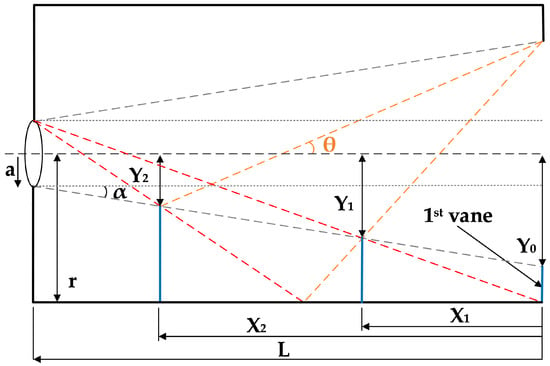
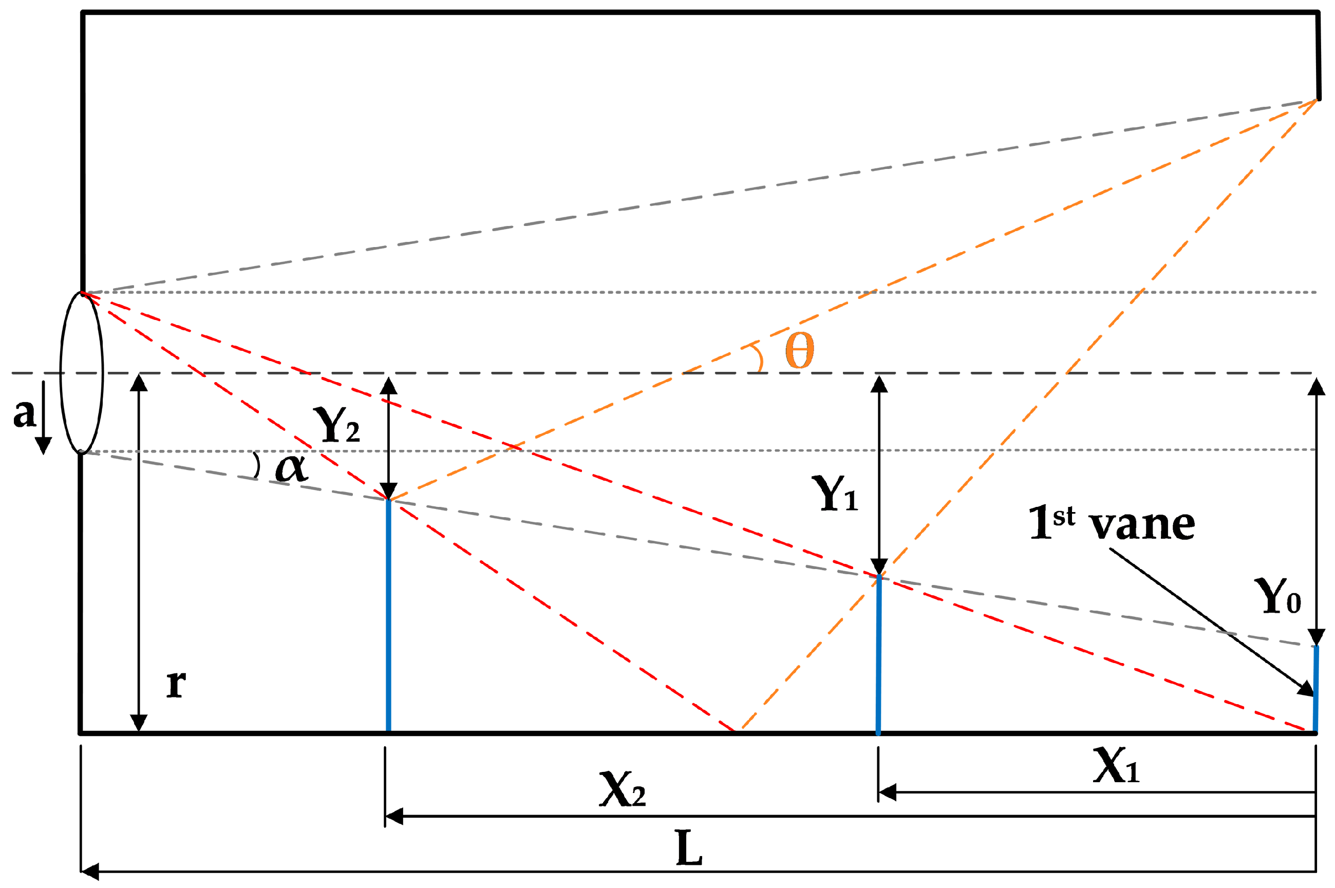
The initial design of the baffle subsystem is based on the vane geometrical location methodology proposed in [13,14]. This approach defines the main vane parameters, namely the axial position $X_n$, the vane inner radius $Y_n$, and a non-dimensional correction parameter $Z_n$, which together describe the geometrical configuration of the baffle. The overall geometry is illustrated in Figure 1. The formulation relies on the limiting stray-light ray connecting the detector-side aperture and the entrance pupil, which defines the constraints for vane positioning and sizing.

Figure 1. Vane arrangement in the baffle system based on the geometrical ray-tracing formulation. The black solid lines represent the baffle geometry and internal walls, while the dashed grey lines indicate reference geometrical limits. The red dashed lines correspond to limiting stray-light rays reaching the detector, and the orange dashed line represents the field-of-view boundary defined by the angle $\theta$. The blue vertical lines indicate the positions of the vane openings, characterized by the geometrical parameters $X_n$ and $Y_n$.

3.1.1. Limiting Ray Geometry

Considering a two-dimensional axial section, the limiting ray is defined between the detector-side opening of radius $Y_0$ at $x=0$ and the entrance pupil of radius a at $x=L$. Assuming straight-line propagation, the ray equation is:

$$\begin{array}{c}\hfill y\left(x\right)=Y_0-{\displaystyle \frac{(Y_0-a)}{L}}x\end{array}$$

(1)

At the location of vane n, positioned at $x=X_n$, the ray intersects the vane tip at $y=Y_n$. Substituting:

$$\begin{array}{c}\hfill Y_n=Y_0-{\displaystyle \frac{(Y_0-a)}{L}}{X}_n\end{array}$$

(2)

Rearranging, the axial position of vane n is obtained as:

$$\begin{array}{c}\hfill X_n=(Y_0-Y_n){\displaystyle \frac{L}{(Y_0-a)}}\end{array}$$

(3)

3.1.2. Vane Radius Formulation

The vane inner radius $Y_n$ is expressed as a function of the non-dimensional parameter $Z_n$, defined as:

$$\begin{array}{c}\hfill Z_n={\displaystyle \frac{Y_n-a}{r-Y_n}}\end{array}$$

(4)

Solving for $Y_n$:

$$\begin{array}{c}\hfill Y_n=r-{\displaystyle \frac{(r-a)}{(1+Z_n)}}\end{array}$$

(5)

3.1.3. Correction Parameter Definition

The parameter $Z_n$ accounts for the effective visibility of the baffle inner wall through the vane opening. Following the formulation of [13,14], $Z_n$ is defined as:

$$\begin{array}{c}\hfill Z_n={\left[2a{h}_{\mathrm{eff},n}\right]}^{-1}\end{array}$$

(6)

The effective height $h_{\mathrm{eff},n}$ includes two contributions:

• The radial clearance at the detector side, $(r-Y_0)$;
• An axial projection term associated with the vane position $X_n$, scaled by the limiting-ray slope and corrected by the aperture geometry.

Thus, the effective height is given by:

$$\begin{array}{c}\hfill h_{\mathrm{eff},n}=(r-Y_0)+X_n{\displaystyle \frac{(Y_0-a)}{L}}{\displaystyle \frac{(Y_0+r)}{(Y_0+Y_n)}}\end{array}$$

(7)

Substituting into the definition of $Z_n$, the final expression becomes:

$$\begin{array}{c}\hfill Z_n={\left[2a\left((r-Y_0)+X_n{\displaystyle \frac{(Y_0-a)}{L}}{\displaystyle \frac{(Y_0+r)}{(Y_0+Y_n)}}\right)\right]}^{-1}\end{array}$$

(8)

3.1.4. Geometrical Parameters and Application

In this formulation:

• $X_n$ is the axial distance from the entrance pupil to vane n;
• $Y_n$ is the inner radius of vane n;
• $Z_n$ is a non-dimensional correction parameter coupling the geometrical relations.

The method requires as input the entrance pupil radius a, the baffle length L, the internal wall radius r, and the system field-of-view angle $\alpha$ (see Figure 1).

The coupled system of Equations (3)–(8) is solved iteratively to determine the complete vane distribution along the baffle.

3.2. Signal-to-Noise Ratio

The second design verification is to validate the SNR of the selected optical sensor as a function of the solar incidence angle. As in [10], it is defined as given by:

$$SN{R}_{log}(m_v,\theta )=10{log}_{10}\left({\displaystyle \frac{S_{\mathrm{star}}\left(m_v\right)}{N_{\mathrm{total}}(m_v,\theta )}}\right)$$

(9)

where $S_{\mathrm{star}}$ is the total number of electrons generated by the selected star of magnitude $m_v$, and $N_{\mathrm{total}}$ is the total number of electrons received, including contributions from the star, the Sun, electronic readout noise, and dark noise.

The $S_{\mathrm{star}}$ is given by:

$$S_{\mathrm{star}}\left(m_v\right)=b_{\mathrm{factor}}\left(m_v\right)·N_{\mathrm{Vega}}·\tau ·A_{EP}·t·K_{\mathrm{fill}}·{\displaystyle \frac{1}{PS{F}_{\mathrm{pixels}}}}$$

(10)

where $b_{\mathrm{factor}}$ is the conversion factor relating star magnitude to Vega; $N_{\mathrm{Vega}}$ is the electrons per m²·s, provided by Vega (already includes quantum efficiency); $\tau$ is the optical transmittance (≈0.95); $A_{EP}$ is the entrance pupil area; t; is the integration time; $K_{\mathrm{fill}}$ is the detector fill factor ($0.87$ [10]); and $PS{F}_{\mathrm{pixels}}$ is the pixel count of the point spread function (9 px).

The total number of electrons received, including contributions from the star, the Sun, electronic readout noise, and dark noise $N_{\mathrm{total}}$, is given by:

$$N_{\mathrm{total}}(m_v,\theta )=\sqrt{S_{\mathrm{star}}\left(m_v\right)+PST\left(\theta \right)·B_{\mathrm{sun}}+{\left(\sum N_{\mathrm{ele}}\right)}^2}$$

(11)

where $PST\left(\theta \right)$ is the baffle’s PST as a function of solar incidence angle $\theta$, $B_{\mathrm{sun}}$ is the number of electrons from solar radiation and $\sum N_{\mathrm{ele}}$ is the combined electronic readout and dark noise.

The $PST\left(\theta \right)$ is defined as the ratio of the irradiance $E_{Sensor}\left(\theta \right)$ measured on the imaging surface of the optical detector and the irradiance $E_{Sun}\left(\theta \right)$ at the input baffle aperture referenced to the point source is given by:

$$PST\left(\theta \right)={\displaystyle \frac{E_{Sensor}\left(\theta \right)}{E_{Sun}\left(\theta \right)}}$$

(12)

Model Validation Considerations

The signal-to-noise ratio (SNR) formulation adopted in this work is based on established approaches for evaluating stray-light suppression performance in star sensors, as reported in [10].

It should be noted that, in the present study, the SNR model is used as a predictive tool during the preliminary design phase of the instrument. Although this formulation has been validated in previous studies, a direct validation for the specific optical configuration proposed in this work has not yet been performed.

Such validation requires dedicated laboratory testing under controlled illumination conditions, as well as correlation with in-orbit data. These activities are foreseen in future work to further consolidate the performance assessment of the proposed dual-purpose instrument.

3.3. Fastener Thermal Modelling

The total thermal resistance on the fastener, i.e., fasteners, surface contact and connecting elements, is given by:

$${\displaystyle \frac{1}{R_{\mathrm{mech}\mathrm{joint}}}}={\displaystyle \frac{1}{R_{\mathrm{flange}}}}+{\displaystyle \frac{1}{R_{\mathrm{fastener}}}}$$

(13)

where $R_{\mathrm{mech}\mathrm{joint}}$ is the thermal resistance of the mechanical joint interface (a conservative approach would be considering smaller area), and its equation is as follows:

$$R_{\mathrm{flange}}=R_{\mathrm{flange}\mathrm{material}}+R_{\mathrm{flange}\mathrm{contact}}$$

(14)

$R_{\mathrm{fastener}}$ is the thermal resistance of the bolt with the associated washers as shown in the next equation:

$$R_{\mathrm{fastener}}=R_{\mathrm{washer}\mathrm{contact}}+R_{\mathrm{washer}}+R_{\mathrm{bolt}}+R_{\mathrm{bolt}\mathrm{head}\mathrm{contact}}$$

(15)

The contact thermal resistance of the $R_{\mathrm{contact}}$ values was obtained based on the curve fitted function $h_c$ (16) and multiplied by the contact area $Are{a}_{\mathrm{contact}}$, as given by:

$$h_c=21.155T^3-54.406T^2+275.078T+661.119$$

(16)

$$R_{\mathrm{contact}}={\displaystyle \frac{1}{h_c·Are{a}_{\mathrm{contact}}}}$$

(17)

The thermal sensitivity was determined in order to understand the uncertainty of the simulated values used. In order to calculate this uncertainty margin, the “Classical uncertainty analysis” defined in [15] is used and is given by:

$$\Delta {\varphi }_i=\sqrt{{\displaystyle \sum _{j=1}^{n_s}}{\left(\Delta {\varphi }_{r,j}\right)}_i^2}+{\left(\Delta {\varphi }_s\right)}_i$$

(18)

where $\Delta {\varphi }_i$ is the overall uncertainty on model output i; ${(\Delta {\varphi }_{r,j})}_i^2$ is the uncertainty due to statistical parameters j on model output i; and ${(\Delta {\varphi }_s)}_i$ is the systematic uncertainty on model output i, usually considered as 3 °C bias.

4. Baffle Design

The first baffle design iteration was initiated with the selection of three key components, i.e., the image sensor, the lens system and the CPU. With these three important components, there was necessary information to achieve a mature design. The image sensor information is presented in [9].

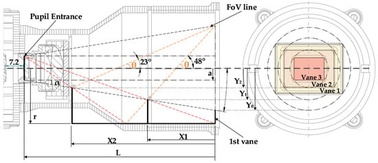
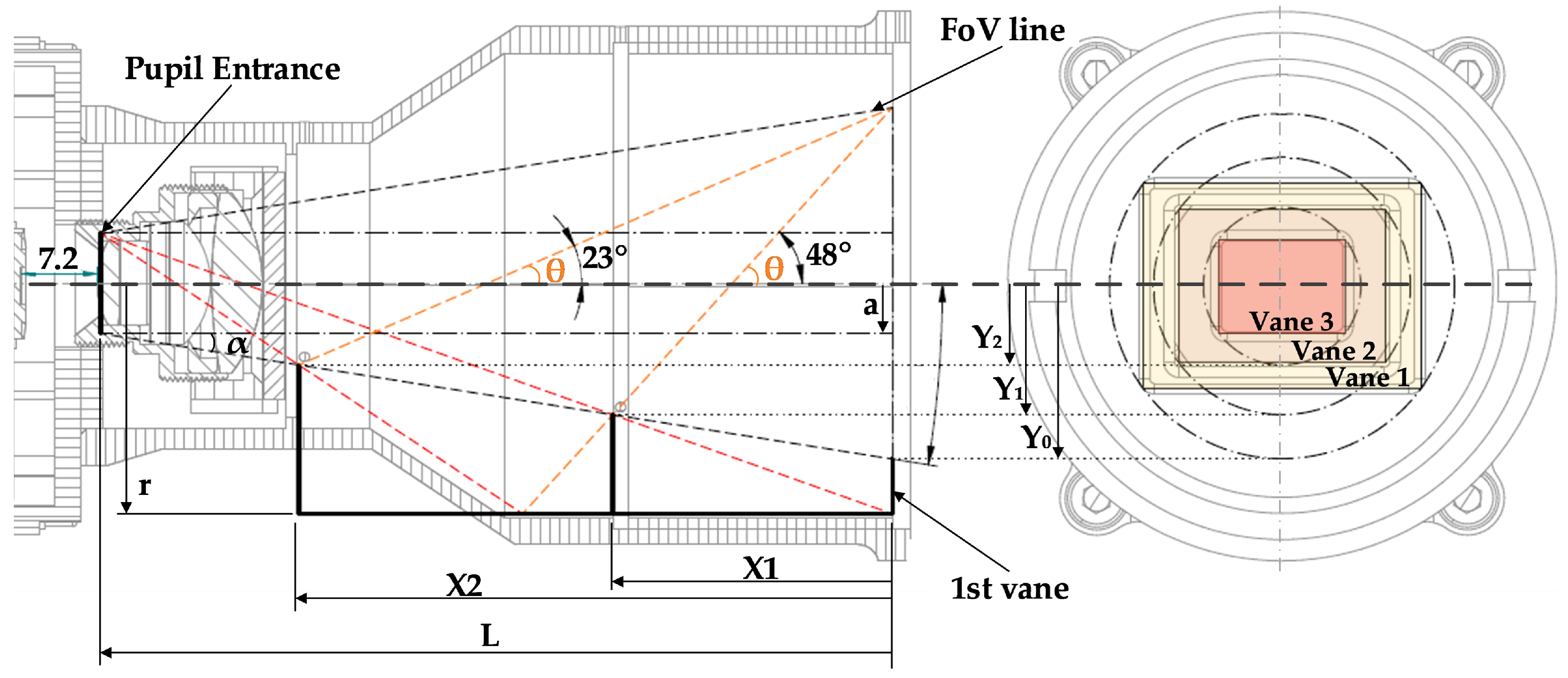
One of the important features of this STR design is the radiation-hardened window that is used to protect the COTS lens, in order to avoid obscuration and radiation damage. The vanes’ geometrical location size, defined by the methodology in (3), (5) and (8) and described by [13,14], is shown in Figure 2.

Figure 2. Baffle system vane arrangement with conceptual ray tracing. The left view shows the axial section of the baffle, where the black solid lines represent the structural geometry, the red dashed lines indicate limiting stray-light paths reaching the detector, and the orange dashed lines correspond to the field-of-view (FoV) boundary defined by the angles $\theta$, 23°, and 48°. The positions of the vanes are defined by the geometrical parameters $X_n$ and $Y_n$. The right view presents a frontal section of the baffle, illustrating the relative positions of Vane 1, Vane 2, and Vane 3 with a square aperture.

The application of the previous equations leads to the mechanical design in Figure 2 for the baffle.

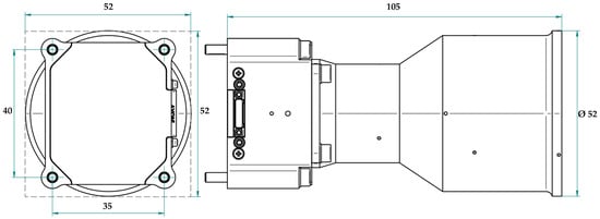
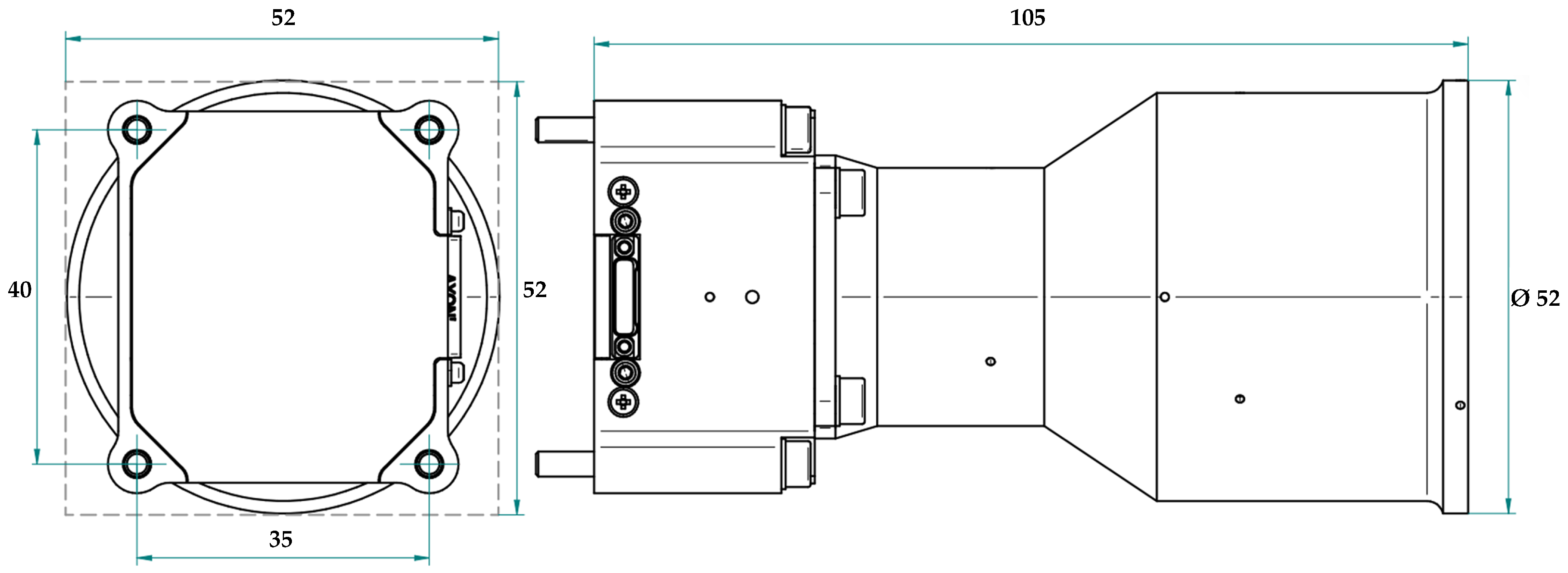
One of the major requirements was for the design of the space camera to be as small and light in mass as possible, leading to envelop values of 105 mm × 52 mm × 52 mm and a mass of 172.58 g.

In order to provide a clearer overview of the system-level design, a mass budget breakdown of the STR is presented in Table 1. The components have been grouped by subsystem to improve readability.

Table 1. Mass budget breakdown of STR.

Subsystem	Mass (g)	Contribution (%)
Baffle assembly (including vanes and spacers)	73.61	42.7
Optical components (lens + radiation window + mount)	19.45	11.3
Structure (enclosure + lid)	39.25	22.7
Electronics (PCBs and components)	21.14	12.2
Mechanical hardware (screws, washers, spacers, pins)	19.13	11.1
Total	172.58	100

The results show that the baffle assembly represents the largest contribution to the total mass, accounting for approximately 42.7% of the system. The remaining mass is distributed between structural elements, optical components, electronic subsystems, and mechanical hardware. This distribution reflects the design trade-offs required to achieve high stray-light suppression performance while maintaining a compact and lightweight architecture suitable for small satellite applications.

The camera body and baffle are made from aluminium and are fixed mechanically with four M3 screws in a rectangular pattern shown in Figure 3.

Figure 3. Mechanical interface and volume envelope. The dashed frame indicates the overall bounding box used to define the maximum external dimensions of the instrument.

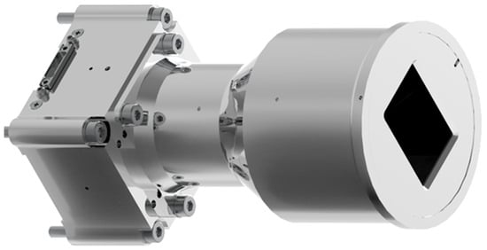
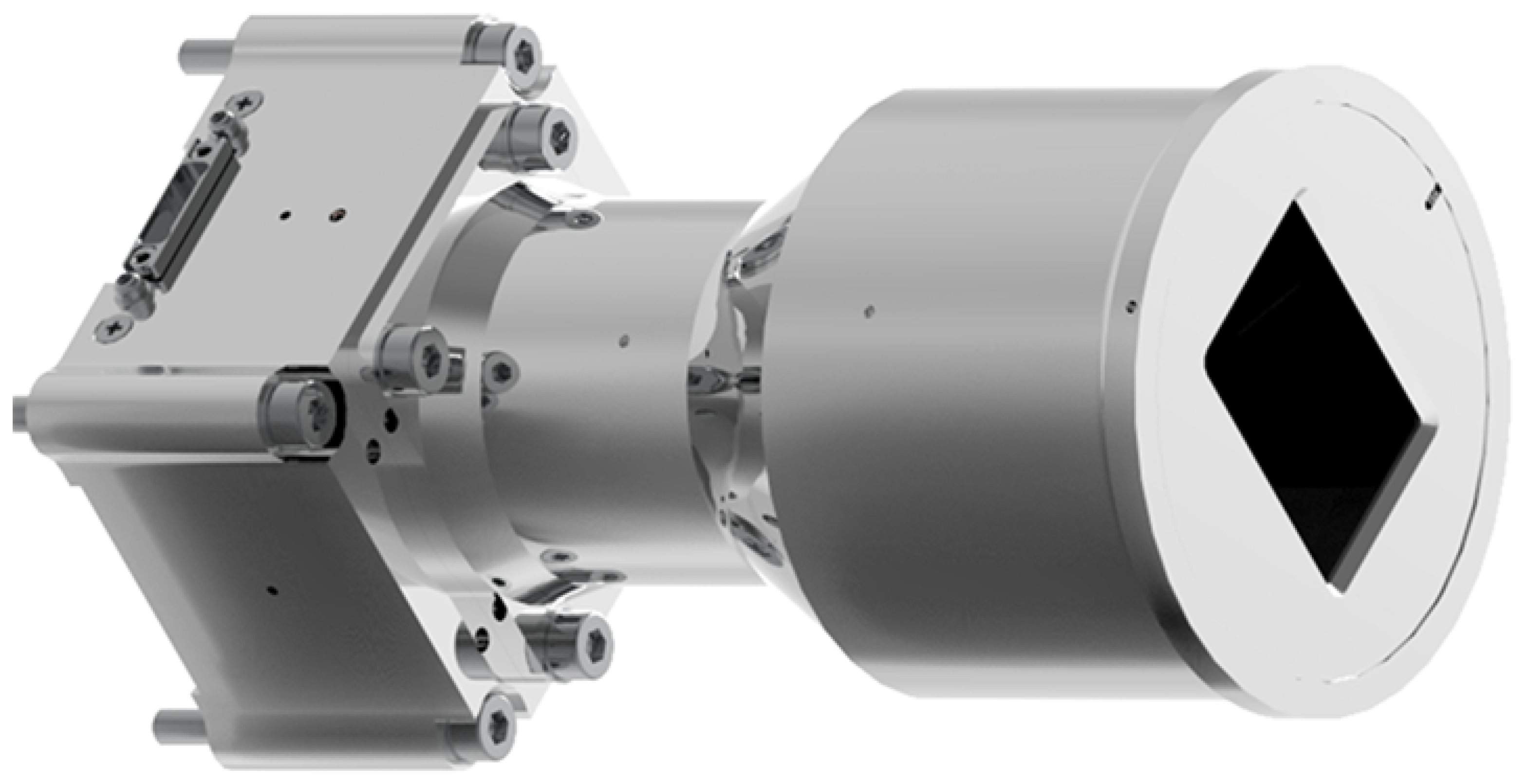
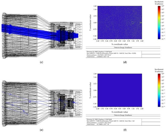
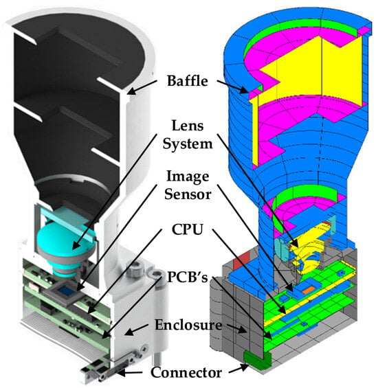
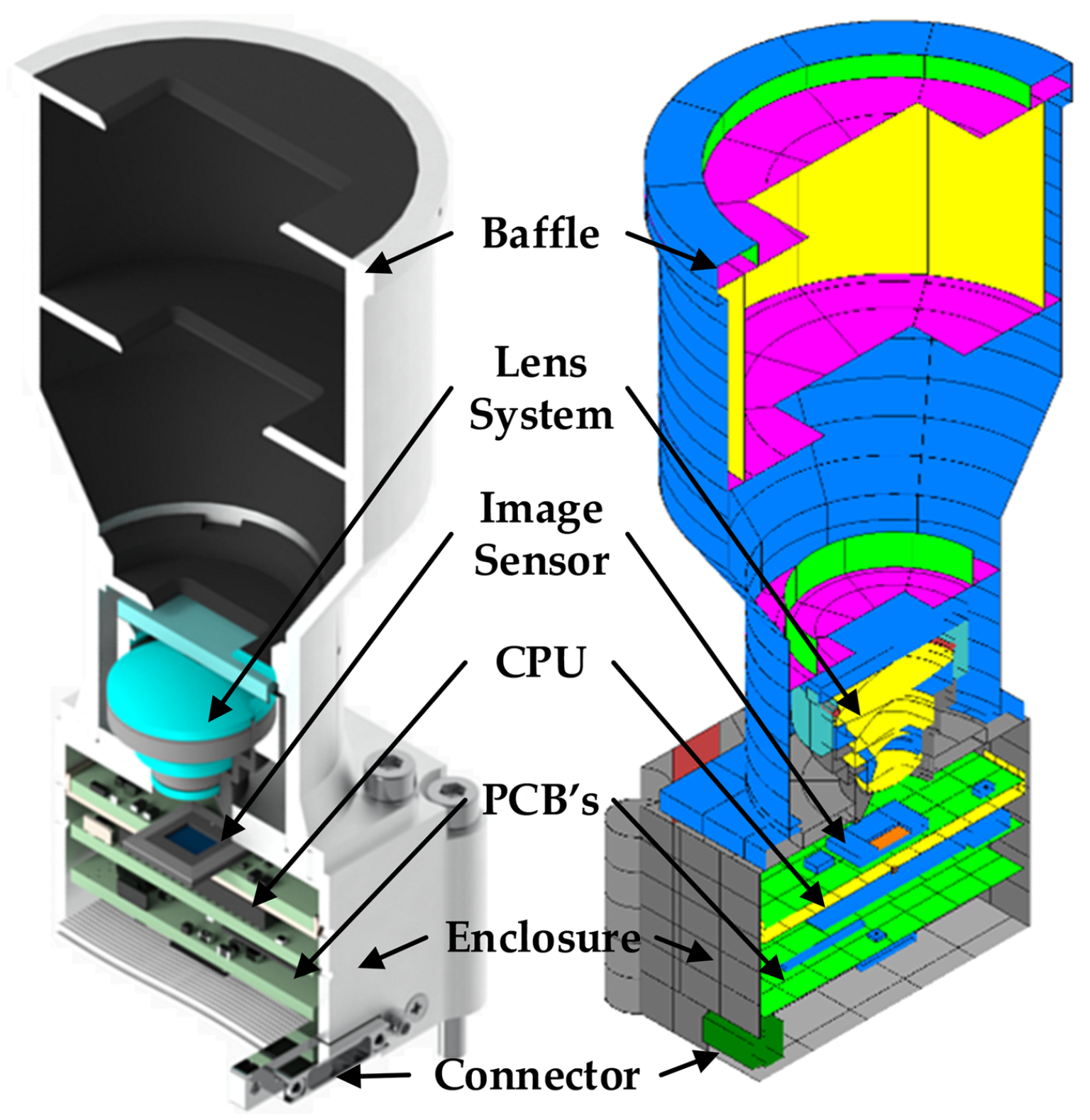
As Figure 4 shows, the camera design is composed of a baffle with three vanes, a lens system with an ionizing radiation-hardened window, a nano D connector, an enclosure body, an image sensor and a CPU with a respective printed circuit board (PCB) [16]. The internal surface of the baffle is top coated with black paint with a light scattering effect due to its roughness, in order to help reduce the stray light coming from the Sun and Earth.

Figure 4. 3D CAD engineering model.

5. Simulation Results

The performance of the Miniaturized Dual-Purpose Camera was assessed through three key simulation domains: optical, thermal, and structural. These simulations were essential to verify that the design met its functional, environmental, and qualification requirements prior to hardware testing.

Each simulation domain was tailored to address the specific operational and environmental constraints encountered in low Earth orbit (LEO), especially for small satellites facing tight mass, volume, and cost budgets. The simulations focused on validating the camera’s stray-light suppression capability, thermal stability across worst-case orbital conditions, and mechanical robustness under launch loads.

• Optical simulations assessed stray-light suppression performance via ray-tracing simulation on ZEMAX and quantified the sensor’s SNR across solar incidence angles, ensuring reliable star tracking and debris detection functionality;
• Thermal simulations were performed using a lumped-parameter model developed in ESATAN-TMS software, version 2024, evaluating the internal component temperatures under hot and cold operational scenarios, including direct solar exposure and power dissipation extremes;
• Structural simulations focused on evaluating the mechanical integrity of the system using finite element analysis (FEA) in NASTRAN software FEMAP™ 2401. Quasi-static, random vibration, and shock spectrum profiles were applied to verify compliance with structural requirements and to estimate the system’s modal characteristics and margins of safety.

The following subsections present detailed results from each simulation domain, demonstrating that the camera meets or exceeds its performance and qualification targets in terms of optical sensitivity, thermal margins, and structural robustness.

5.1. Optical Simulation

The performance of the designed baffle in Figure 2 required a stray-light study involving optical ray tracing simulations for that specific baffle geometry and astronomic radiometer analysis.

5.1.1. Ray Tracing

Optical baffles are typically characterized by a transfer function known as the PST, as demonstrated in [3,10,13,17,18,19,20]. The PST describes the level of attenuation for light entering the system at various incidence angles from external sources such as the Sun, Earth, and Moon.

To evaluate the PST performance of the designed baffle, a series of optical ray-tracing simulations were conducted using ZEMAX™ 14.2 software in non-sequential mode. These simulations modelled sunlight entering the baffle cavity from Figure 2 at different incidence angles, corresponding to three distinct field-of-view directions: maximum horizontal, maximum vertical, and maximum diagonal angles of the optical sensor.

The surfaces of the baffle cavity (Figure 2) are top coated with a black paint, Aeroglaze Z306, which is considered to have a total integrated scatter (TIS) value of 3%; i.e., 97% of intensity of the ray is transmitted and 3% is reflected (the material of the mechanical component is set to MIRROR in the NSCE so no light can be transmitted, so effectively 97% is absorbed and 3% is reflected). The Scatter Fraction of 0.9 means that 90% of reflected rays are scattered according to Lambertian scatter model distribution.

This approach was adopted because the baffle design incorporates vanes shaped with rectangular masks, which are optimized to achieve maximum attenuation and an improved PST response across the optical sensor for the horizontal, vertical, and diagonal field angles.

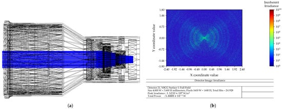
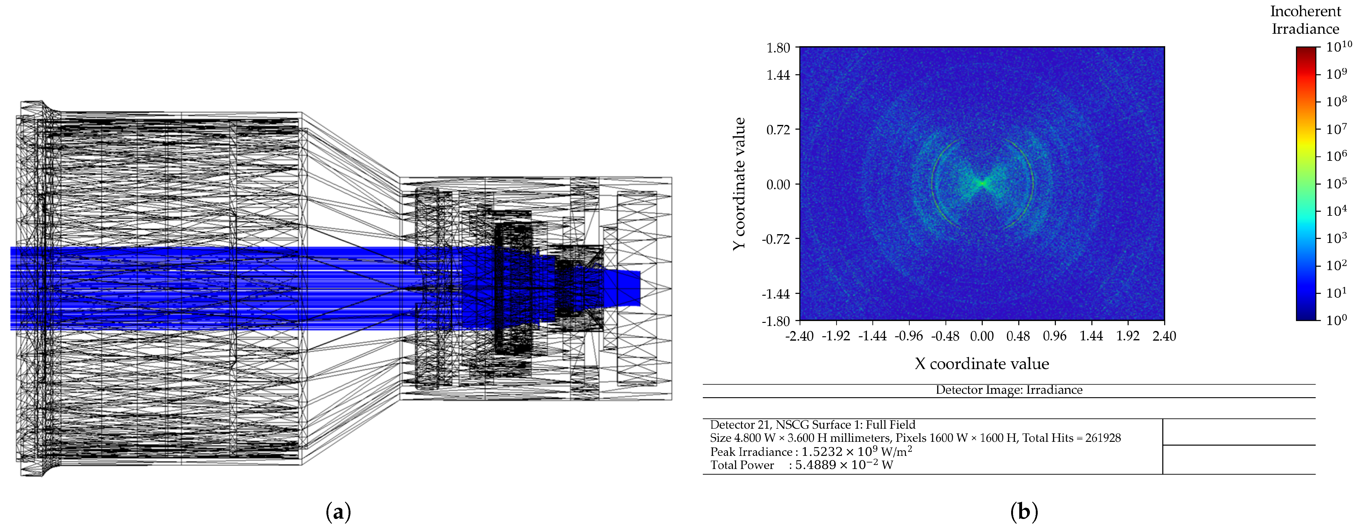
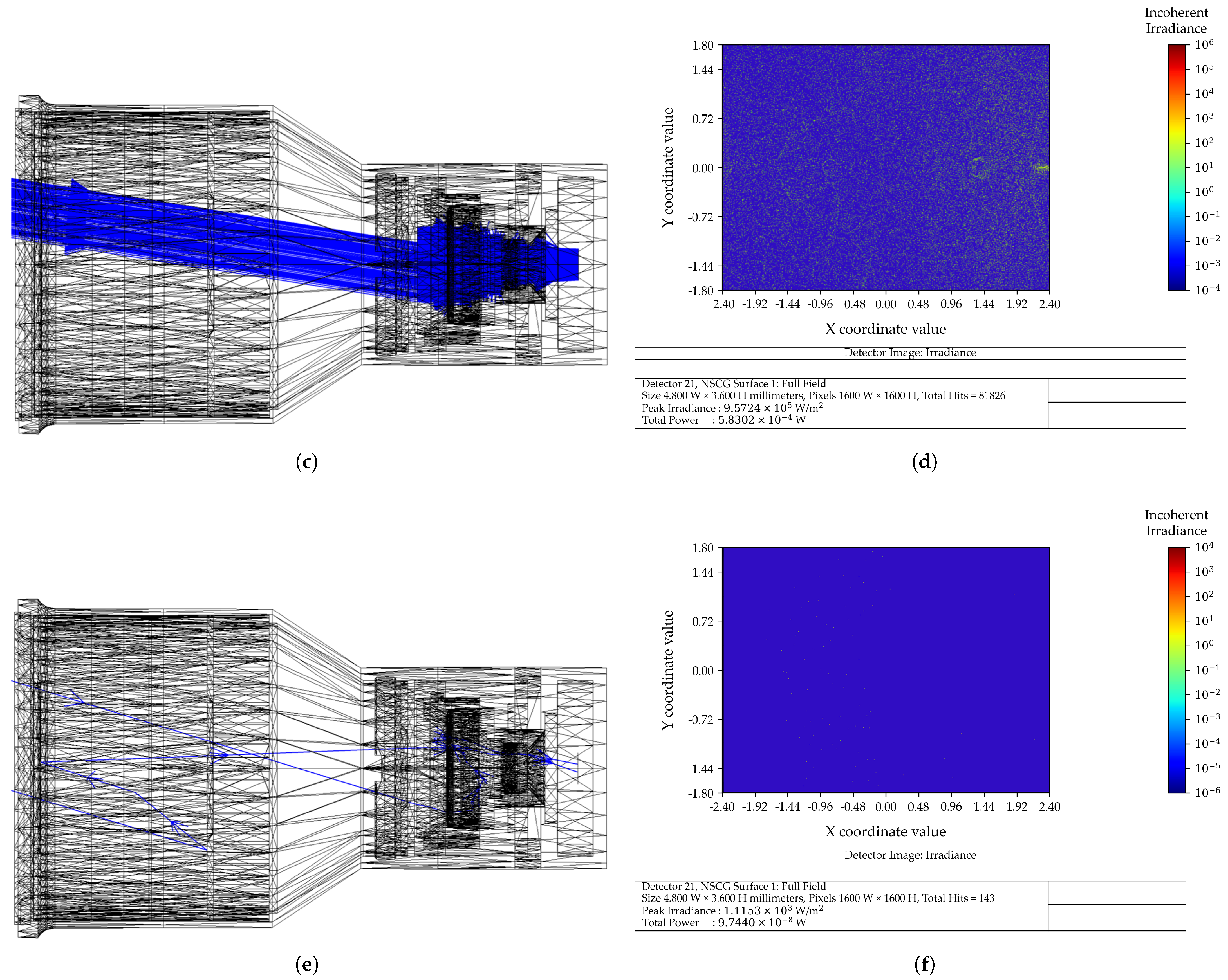
In Figure 5, we show the ray-traced simulation with the respective measured sun irradiance (W/m²) coming from direct and reflected sunlight values, for three different incident angles, i.e., 0° (representing direct sunlight), 9° (representing the maximum FoV) and 23° (representing direct sunlight). This last angle (23°) corresponds to the cut-off condition, beyond which direct solar radiation no longer impinges on any optical component, such as the radiation-hardened window.

Figure 5. Ray-tracing simulations for the horizontal field of view: (a,c,e) ray tracing for θ = 0°, 9°, and 23°, respectively; (b,d,f) corresponding detector irradiance on logarithmic scale (W/m²).

The results show a progressive reduction in irradiance with increasing incidence angle, highlighting the effectiveness of the baffle in suppressing stray light. For every field angle a specific amount of solar irradiation is absorbed by the optical sensor, and with this measurement it is possible to construct the PST optical transfer function $PST\left(\theta \right)$ used in [6].

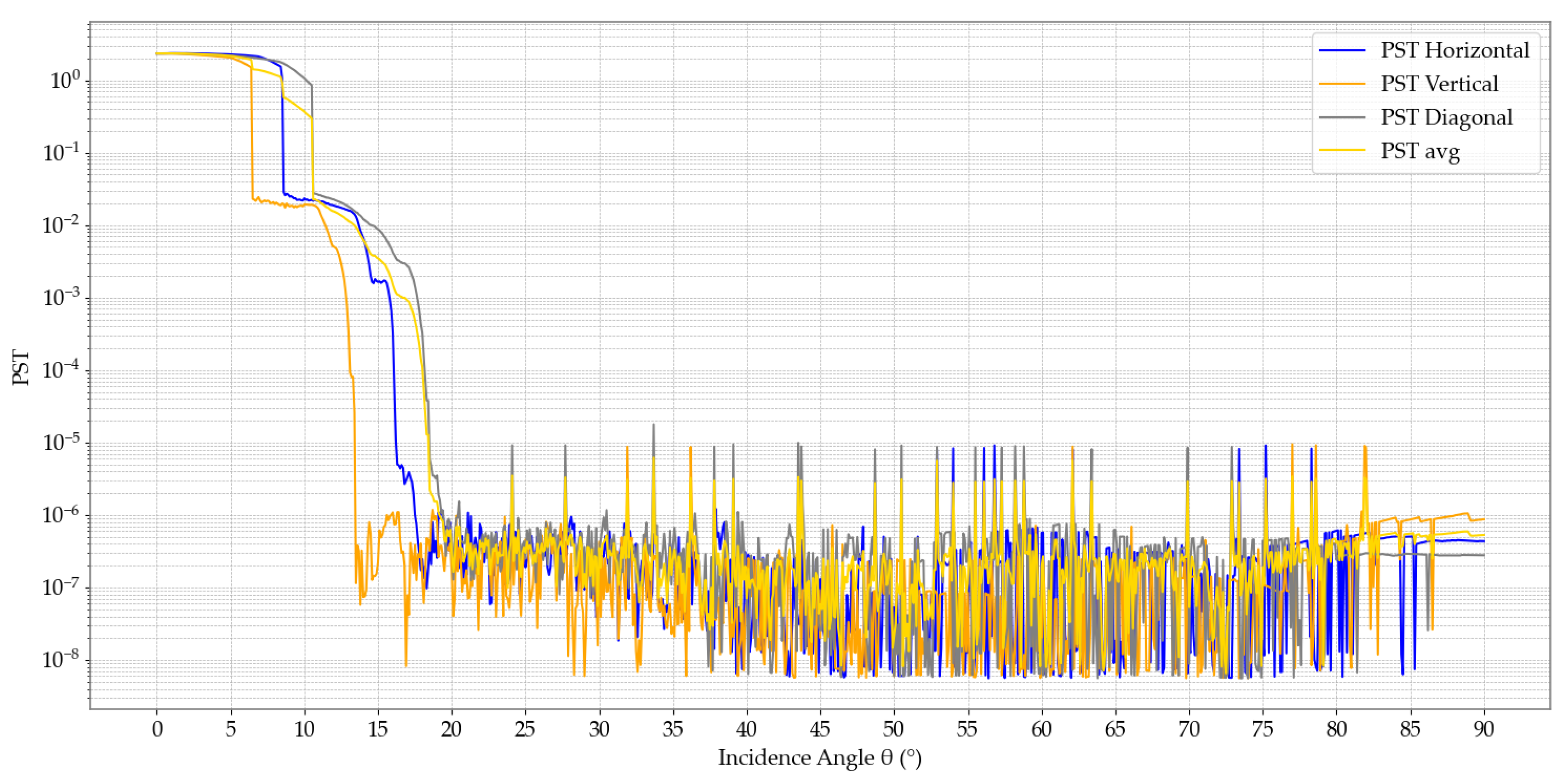
Considering [7], performing the ray-tracing simulations and post-processing the PST response across the optical sensor for three configurations, i.e., horizontal, vertical, and diagonal field angles, we obtain three PST functions, i.e., $PS{T}_{Hor}\left(\theta \right)$, $PS{T}_{Ver}\left(\theta \right)$ and $PS{T}_{Dia}\left(\theta \right)$, respectively, as shown in Figure 6.

Figure 6. Point Source Transmission (PST) as a function of the solar incidence angle for horizontal, vertical, diagonal fields of view and the average between them all.

Figure 6 shows a sharp decrease in PST between approximately 10° and 20°, which indicates the effectiveness of the baffle in attenuating stray light, defining the practical sun exclusion angle of the system.

5.1.2. SNR Results

For the SNR analysis, the average $PST\left(\theta \right)$ was calculated ($PS{T}_{avg}\left(\theta \right)$), as shown in Figure 6, and then interpolated considering [6]. With this, it is possible to estimate the $SN{R}_{log}(m_v,\theta )$, considering [4], for a desired magnitude $m_v$ of a Star and for a specific integration time t of the optical sensor. Other optical parameters for the SNR model are presented in Table 2; the data presented were determined in the laboratory or extracted from respective datasheets. The laboratory is at Synopsis Planet, Faculdade de Ciências, Universidade de Lisboa, Portugal.

Table 2. Optical sensor characteristics for SNR analysis.

Parameter	Value
Pixel N° width	1280
Pixel N° height	960
Readout noise ($e^{-}$)	0.797
Dark noise ($e^{-}$/s)	2.4
Lens focal distance (mm)	16
Pixel size ($\mathsf{\mu }$m, square)	3.75
PSF pixels	9
Entrance pupil diameter (mm)	9.5
$\tau$ optical transmittance	0.95

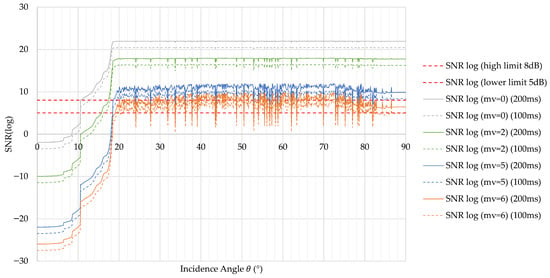
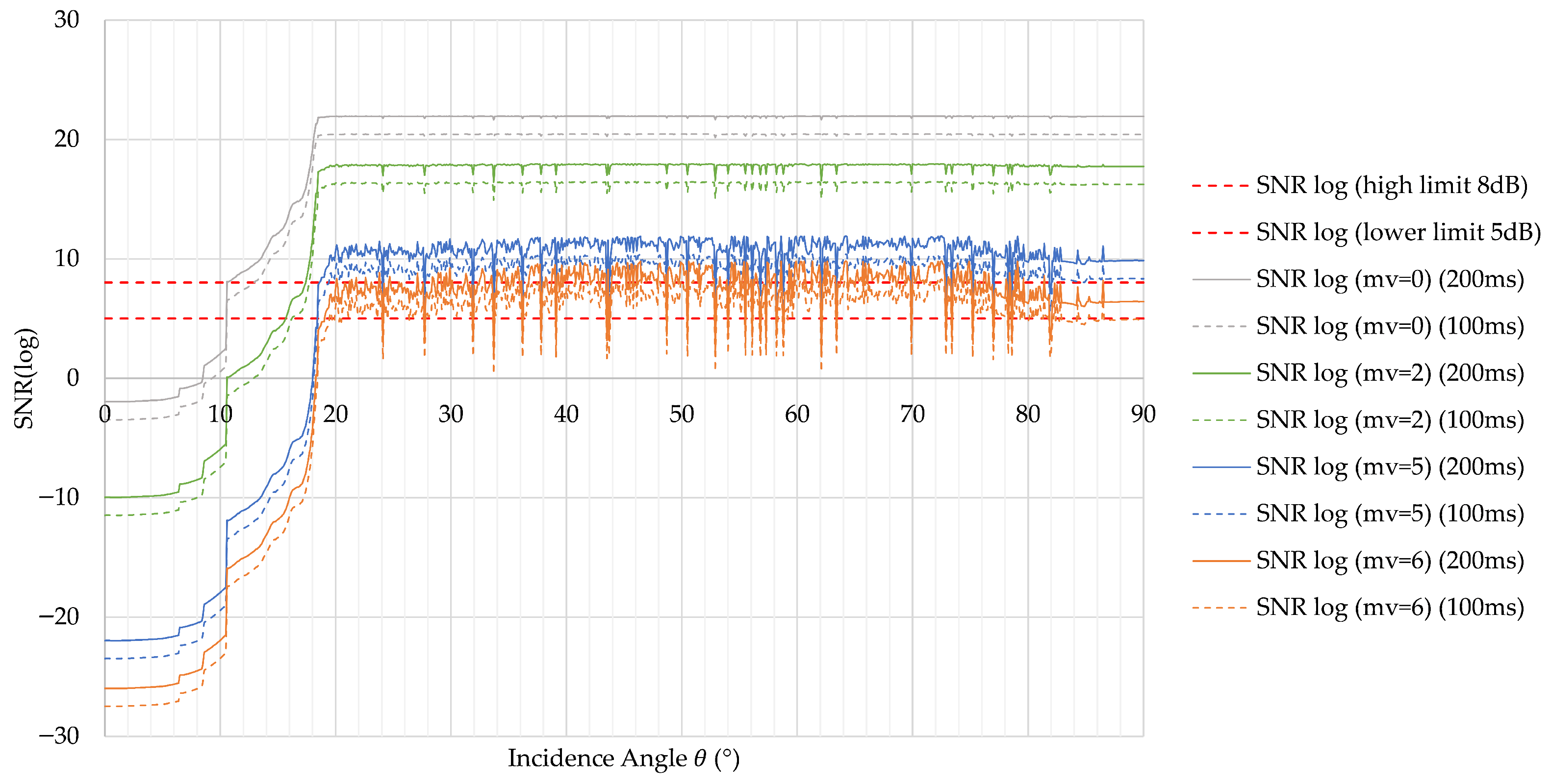
With this information, it is possible to build detailed curves of the sensor performance for a specific space condition in space, where multiple magnitudes of stars can be seen. The different incident angles of the Sun that affect the instrument $SN{R}_{log}(m_v,\theta )$ are shown in Figure 7, where different magnitudes of star values are used, from 0 to 6, and two distinct integration times are used: 100 ms and 200 ms.

Figure 7. Logarithmic ${\mathrm{SNR}}_{log}$ as a function of the solar incidence angle for different star magnitudes and integration times (100 ms and 200 ms).

The results show that the SNR increases significantly beyond approximately 20°, where stray-light influence is reduced, enabling reliable detection of stars up to magnitude ∼5.8.

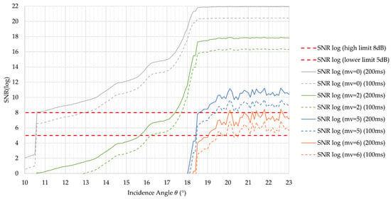
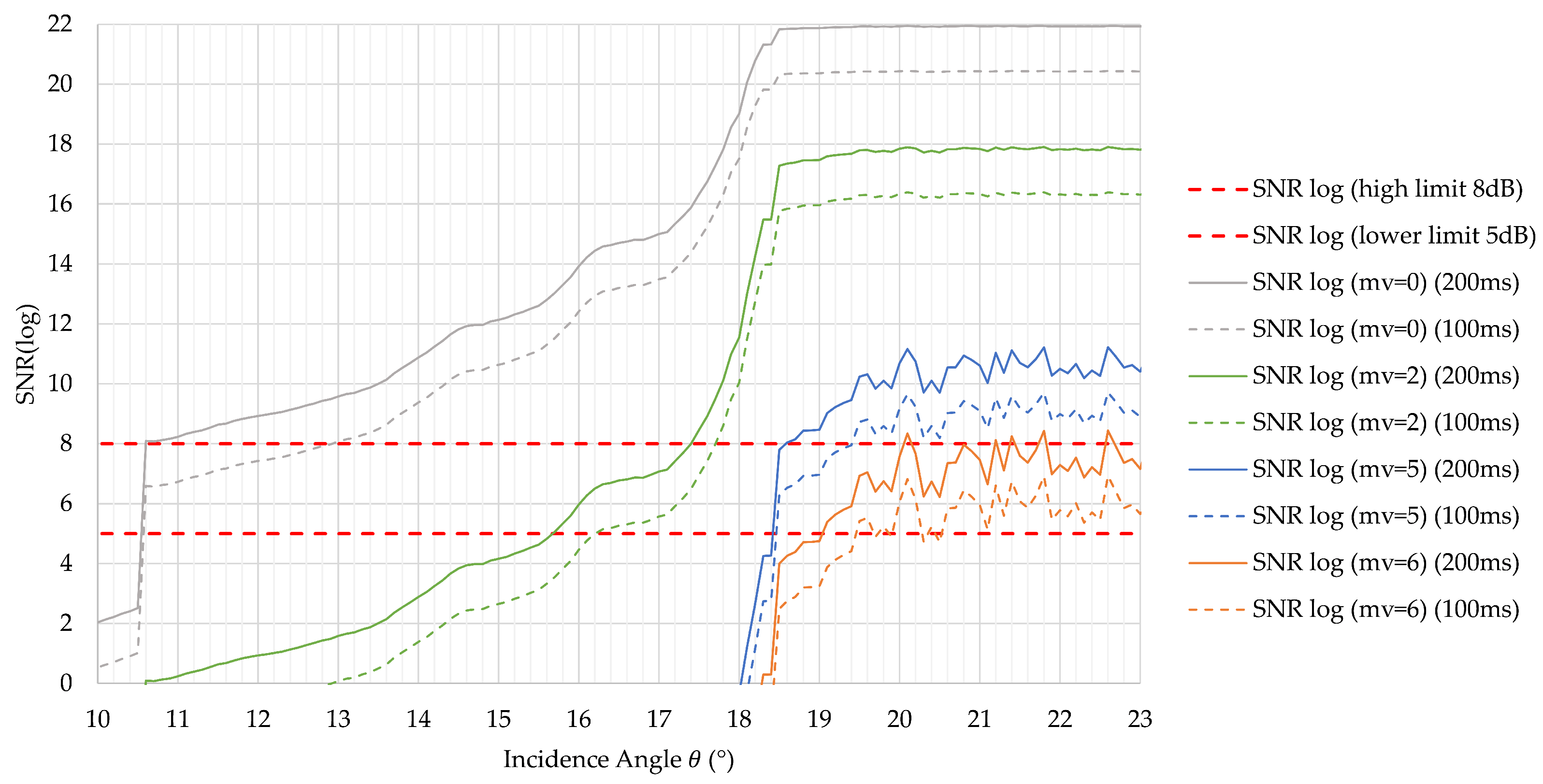
It is visible that the baffle transfer function plays an important role in the SNR value. At an incidence angle value of 90°, meaning that no sunlight comes into the baffle, the SNR is at its maximum value for a considered plateau of incidence angle values $\theta$ ranging from 20° to 90°, while at 0°, meaning that the Sun is hitting the optical sensor directly perpendicularly, even the bright Vega star has a negative SNR, meaning that the entire sensor is blind. Only after reaching a sun incidence angle of 9° does the Vega star start to have positive SNR values. If we look at Figure 8, we can see in more detail the SNR values between the camera-designed FoV value of 9° and the baffle direct Sun cut-off angle of 23°; we can identify clearly the most effective incidence angle, which we can consider as corresponding to the best sun exclusion angle.

Figure 8. Detailed view of ${\mathrm{SNR}}_{log}$ in the critical angular range between 10° and 23°.

The transition from negative to positive SNR values highlights the minimum sun exclusion angle required for effective star detection, with SNR thresholds of 5–8 dB achieved near ∼19°. As indicated in [9], the image sensor must have a minimal SNR value of between 5 and 8; therefore, we can assume that with this current baffle design with integration times between 100 ms and 200 ms, it is possible to detect stars up to 5.85 in magnitude in order to use detection software like the Tetra algorithm, ASTRiDE and the new hybrid time-indexed method, as demonstrated in [4,5,6,7,8].

5.2. Thermal Simulations

A lumped-parameter method (LPM)—thermal model—was developed to validate the thermal performance of the instrument in different worst-case scenarios. Hence, this method could influence the stress on the instrument in extreme space environmental conditions.

5.2.1. LPM Description

A lumped-parameter model (LPM) with 1596 nodes was developed for the Dual-Function Camera using ESATAN-TMS software (version 2024). Figure 9 presents a comparison between the 3D CAD model and the corresponding Thermal Geometric Mathematical Model.

Figure 9. 3D Section Views: CAD model (left) and Thermal Geometric Mathematical Model (right).

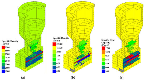
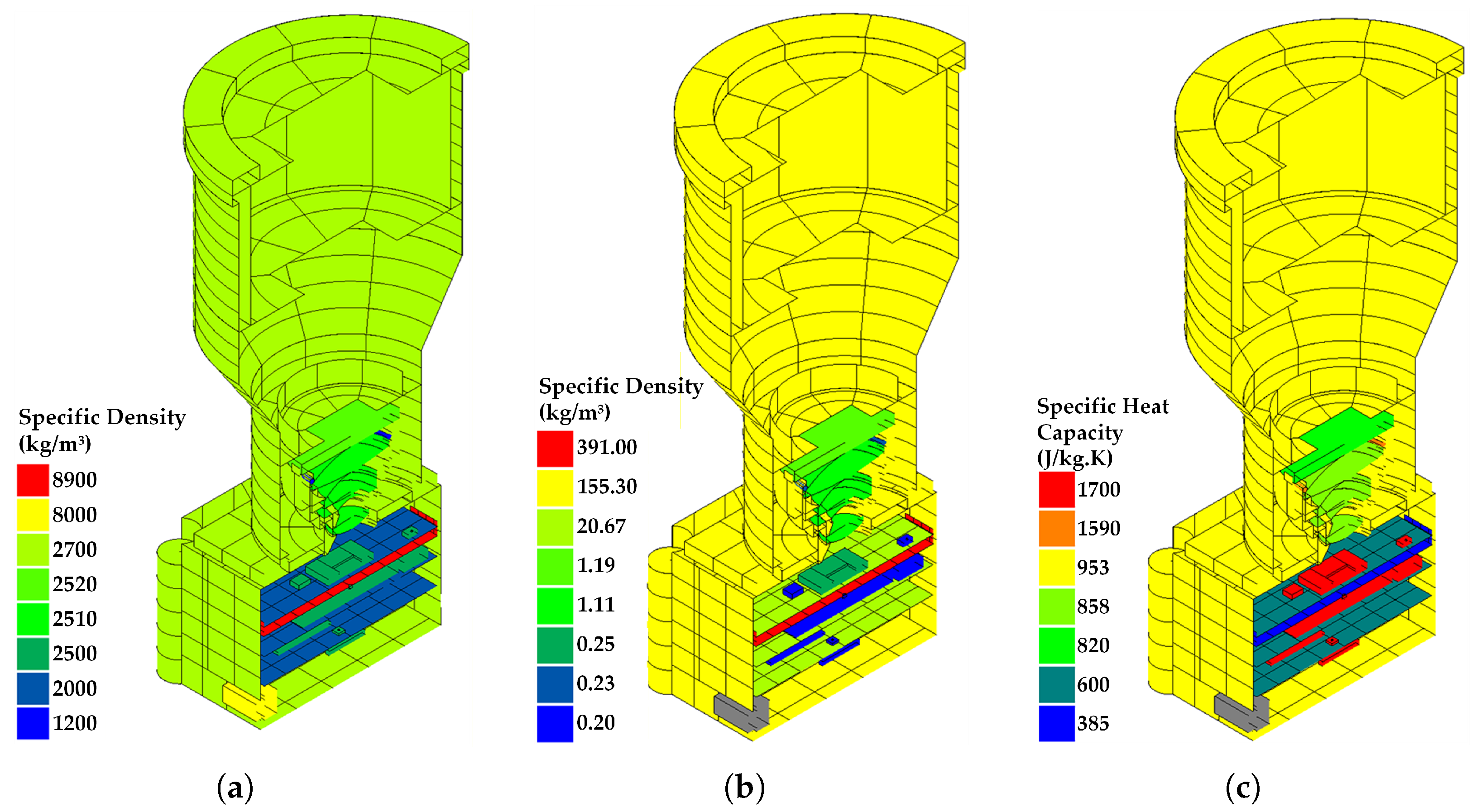
The main structure, enclosure, and baffle of the optical instrument are manufactured from aluminium alloy. Other components include flame-retardant FR4 for the PCBs, glass for the lens system, plastic and ceramic materials for selected EEE components, and copper for the CPU heat sink. Figure 10 presents the material properties used in the model: (a) specific density (kg/m³), (b) thermal conductivity (W/m · K), and (c) specific heat capacity (J/(kg · K)).

Figure 10. Material properties of the thermal model: (a) specific density (kg/m³); (b) thermal conductivity (W/m · K); (c) specific heat capacity (J/(kg · K)).

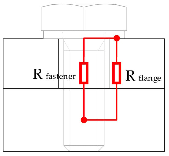
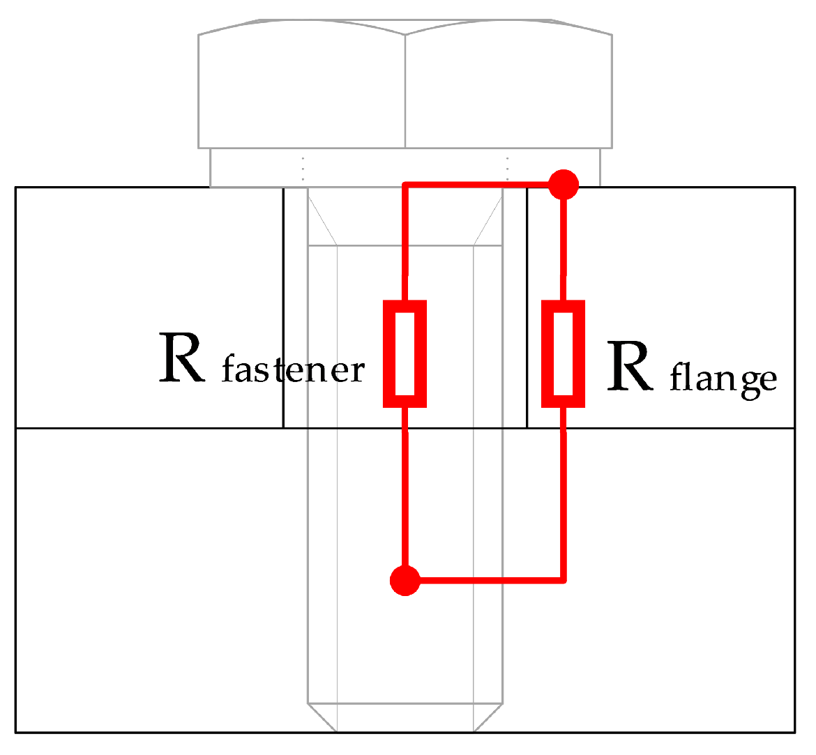
The heat-transfer path across bolted interfaces comprises both the fastener body and the surface-contact region, represented in Figure 11 as $R_{\mathrm{fastener}}$ and $R_{\mathrm{flange}}$. The total thermal resistance of each mechanical joint, $R_{\mathrm{mech},\mathrm{joint}}$, is evaluated using Equations (13)–(15). The internal thermal conductances (W/K) are derived from compression-contact conductance values (W/m²K), combined with the geometric and material properties of the bolt and flange.

Figure 11. Heat path through bolted joints.

The thermal contact conductance, $h_c\left(T\right)$, is obtained by curve-fitting torque-dependent data from [21], where the applied torque T (N·m) is set to the maximum allowable value for the selected fastener, as defined in Equation (16). Using this formulation, the resistances $R_{\mathrm{fastener}}$ and $R_{\mathrm{flange}}$ are computed through Equations (14) and (15), based on the corresponding contact area $Are{a}_{\mathrm{contact}}$, defined in Equation (17).

For clarity, Table 3 summarizes the main thermal resistances. To enhance readability, conductors sharing identical values or modelling assumptions were grouped into representative categories. This approach emphasizes the relative importance of the dominant conductive paths in the model, including optical interfaces, structural fasteners, PCB stack connections, and component-level thermal couplings.

Table 3. Summary of representative thermal resistances used in the ESATAN model.

Conductor Group	R (K/W)	Qty.	Model Application
PCB copper rings	12.29	12	Local conductive links through PCB copper rings
External connector I/F	10.00	3	Internal and enclosure contact paths of the external connector
Baffle to enclosure bolts M3×8	27.94	4	Baffle fixation to top enclosure
Lid to enclosure bolts M1.6×6	257.40	4	Lid fixation to enclosure side walls
PCB stack bolts (PCB1–PCB2–PCB3) M2.5×16	313.38	4	Conductive paths through bolted interfaces in the stacked PCB structure
PCB3 to enclosure flange M2.5×16	121.65	4	Conductive path between PCB3 and enclosure through the support interface
Mech I/F flange M3×30	19.70	1	Enclosure bottom to spacecraft mechanical interface
Mech I/F bolt M3×30	318.17	1	Enclosure top conductive path to spacecraft interface
Optical sensor-to-case	8.00	1	Optical detector package-to-case conductive path
EEE junction-to-case (B1_U1, B1_IC2)	0.20–0.90	2	Components with the lowest internal thermal resistance and strongest junction-to-case conduction
EEE junction-to-case (B1_U3, B1_U4, B2_U3, B2_U1)	3.30–13.30	4	Components with moderate junction-to-case conductive paths
EEE junction-to-case (B1_U2, B1_U5, B1_U6, B1_U7, B3_U1, B3_U2, B3_U3)	20.00–47.85	7	Components with weaker internal thermal coupling between junction and case
EEE case-to-board (B1_U2, B1_U3, B1_U4, B3_U1, B3_U2, B3_U3)	0.53–2.33	6	Strong conductive coupling from package case to PCB
EEE case-to-board (B3_X1, B1_U6)	17.48–28.57	2	Intermediate conduction from package to PCB
EEE case-to-board (B1_U5, B1_U7, B1_IC2)	24.57–30.86	3	Limited conduction to PCB due to package or footprint constraints

As shown in Table 3, the lowest thermal resistances are internal electronic package paths, whereas the highest resistances correspond to bolted structural interfaces, particularly those involving the lid and PCB fixation points. This distribution is consistent with the modelling strategy adopted in the ESATAN thermal model, where compact and well-defined contact interfaces are represented as efficient conductive paths, while mechanically fastened interfaces are dominated by contact resistance and reduced effective heat-transfer area.

5.2.2. Thermal Results

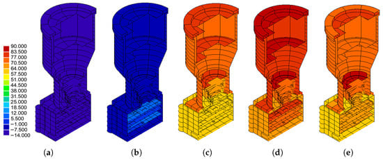
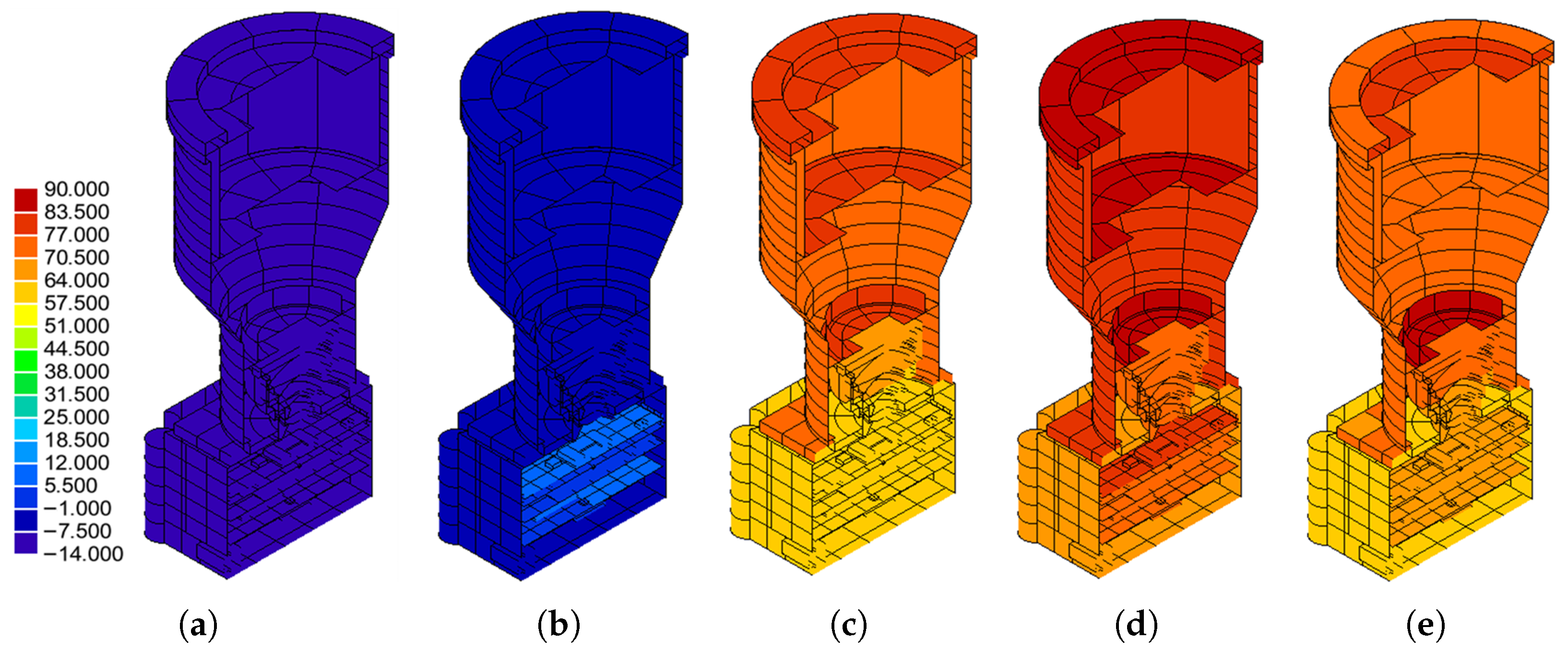
After building a thermal model, a set of simulations for an orbit where the optical camera is configured for different operational modes and different pointing angles relative to the sun were performed. The camera is set to work in two types of thermal cases, Cold and Hot, where the mechanical interface value is between −10 °C and +40 °C. In between these temperature ranges, the idea is to capture the extreme low and high temperatures that eventually the optical instrument will experience; this means that for Cold cases, the camera will not have any power consumption and no external positive heat will increase the temperature, meaning that only the deep space temperature of −270.15 °C influences the final temperatures of the camera. For the Hot case, the idea is to capture the maximum temperatures that the instrument will experience; this means that internal power consumption is set for the maximum power consumption operational case, where it has a maximum power consumption value of 1.499 W, and solar radiation with an incidence angle value of 18.5 °C. For the direct sun thermal case, the sun radiation directly hits the optical sensor, and according to the PST function (Figure 6), it has a total value of 23.4 mW. This will be useful to understand the maximum temperatures reached by the optical sensor if by accident the optical camera faces the sun directly. The temperature maps for the five thermal cases: (a) Cold Non-Operating; (b) Cold Operating; (c) Hot Non-Operating; (d) Hot Operating; (e) Hot Operating—direct sun are shown in Figure 12.

Figure 12. Temperature distribution maps (°C) for five thermal scenarios: (a) Cold Non-Operating case; (b) Cold Operating case; (c) Hot Non-Operating case; (d) Hot Operating case; (e) Hot Operating—direct sun case.

Figure 12 shows that the maximum temperature occurs in the hot operating case with direct sun exposure, highlighting the combined effect of external radiation and internal power dissipation. The minimum temperature value is −14 °C and the maximum temperature value is 90 °C for all five cases. Besides the thermal simulation of the five different thermal cases shown in Figure 12, uncertainty analysis with a total of 16 sensitive cases was also performed, changing the thermal model parameter with typical inaccuracies with a 2-sigma confidence interval, as shown in [15].

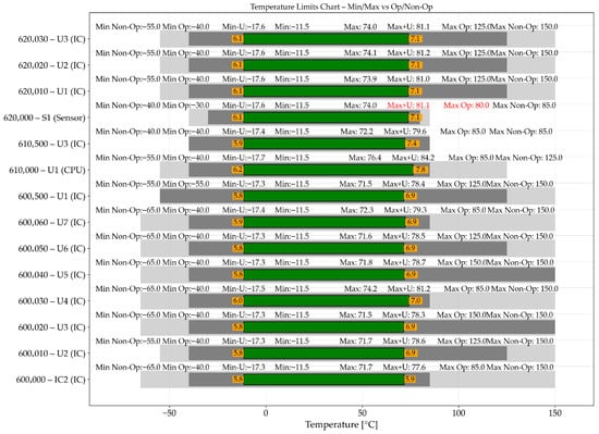
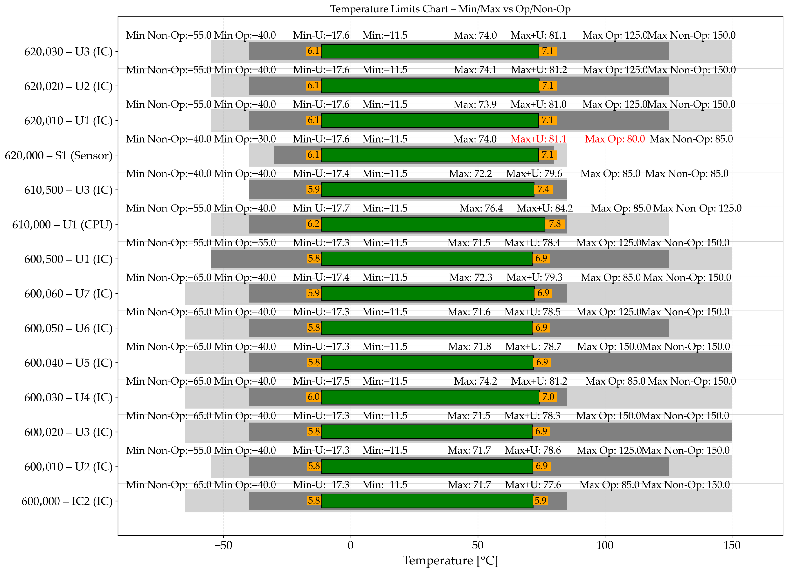
These values are then added to the minimum and maximum value obtain from the five different thermal cases from Figure 12. With these new uncertainty values defined, we can build a “Temperatures Limits Chart” for the main EEE components used by the electronic design shown in [9]. This “Temperatures Limits Chart” is shown in Figure 13.

Figure 13. Temperature limits chart comparing minimum and maximum simulated temperatures (including uncertainty) against operational and non-operational limits of key components. The green bars represent the simulated temperature range, grey regions indicate allowable operational and non-operational limits, orange markers denote minimum and maximum uncertainty margin values, and red annotations highlight temperature limits exceeded.

In Figure 13 we see that all components are within the operational limits, except the optical sensor (Node 620000—S1), which passes the operational limit by +1.1 °C. These results can be considered acceptable at this design stage since the thermal model is not correlated with tests.

It should be noted that the observed temperature exceedance of approximately 1.1 °C for the optical sensor occurs under a worst-case hot scenario, where the instrument is exposed to combined solar and Earth albedo radiation while simultaneously dissipating internal heat from the electronic components, including the image sensor. This behaviour results from the combined effect of internal heat generation and the thermo-optical properties of the external baffle surface, which is currently assumed to be coated with SurTec 650 V. This coating is characterized by a relatively low emissivity ($\epsilon \approx 0.03$) and moderate solar absorptivity ($\alpha \approx 0.42$), leading to increased heat absorption and a reduced capability to radiate heat to space. Potential mitigation strategies include the use of alternative surface treatments with improved thermo-optical properties, such as white thermal control coatings and second surface mirror (SSM) materials (e.g., Teflon tape), or the application of multilayer insulation (MLI). In addition, optimization of the internal heat dissipation paths, including improved conductive coupling to structural elements or dedicated thermal interfaces, may further reduce the sensor temperature. These approaches are expected to improve the thermal balance and bring the sensor temperature within operational limits in future design iterations.

5.3. Structural Simulations

A finite element model (FEM) was developed with a total of 66,240 nodes and 64,455 elements. It was built in NASTRAN, as shown in Figure 14.

The instrument was primarily modelled using the following finite element types:

• Shell elements: used for the baffle, enclosure, printed circuit boards (PCBs), bottom cover, and radiation window, discretized using CQUAD4 elements.
• Solid elements: used for the enclosure and the optical lens system, modelled using CTETRA elements.
• Point masses: representing the baffle vanes, lens system assembly, electrical and electronic equipment (EEE), and mechanical interface (I/F) anchor points, implemented using CONM2 elements.
• Rigid elements: including spring/damper elements for fastened mechanical interfaces and RBE2 elements for local rigid connections. Spring-like behaviour at mechanical interfaces was represented using equivalent stiffness elements derived from bolted joint formulations.

Figure 14. 3D finite element model (FEM) mesh of the STR, illustrating the discretization of the structural components used for structural and dynamic analysis.

Figure 14. 3D finite element model (FEM) mesh of the STR, illustrating the discretization of the structural components used for structural and dynamic analysis.

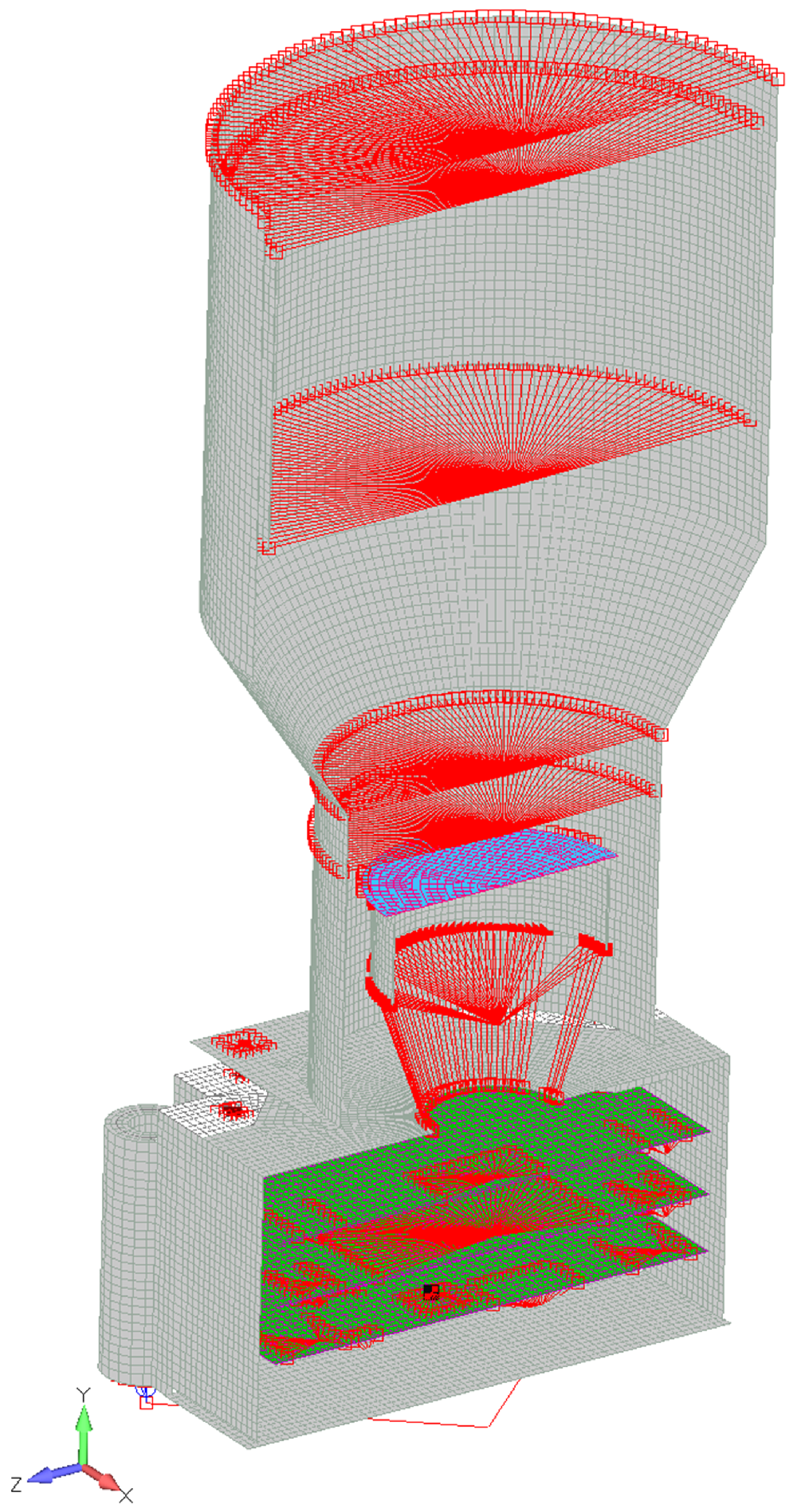
Figure 14 also highlights the modelling strategy adopted to represent both structural and non-structural components, as well as mechanical interfaces. The red markers correspond to rigid link elements (RBE2), which are used to connect lumped masses to the structural mesh and to distribute loads. The green regions represent the printed circuit boards (PCBs), modelled using shell elements (CQUAD4), while the blue regions correspond to the radiation window, also modelled with shell elements (CQUAD4). The grey mesh represents the primary structural components, discretized using a combination of shell (CQUAD4) and solid (CTETRA) elements. Non-structural components, such as the lens assembly and electronic equipment, are represented by lumped mass elements (CONM2), ensuring an accurate representation of the system mass and inertia without excessive mesh refinement.

This hybrid modelling approach allows for an accurate representation of the mass distribution and dynamic behaviour of the system while maintaining a manageable model size and computational cost.

There are three key structural requirements for the design of this optical instrument:

1.

Quasi-Static: a design acceleration load of $20\mathrm{g}$ (1$\sigma$ margin).

2.

Random Vibration: a total acceleration of $14.2{\mathrm{g}}_{\mathrm{RMS}}$ (1$\sigma$ margin), as shown in Figure 15a.

3.

Shock Response Spectrum: acceleration levels reaching up to $1269\mathrm{g}$, as shown in Figure 15b.

Figure 15. Qualification vibration level profiles for all axes: (a) random vibration; (b) shock response spectrum.

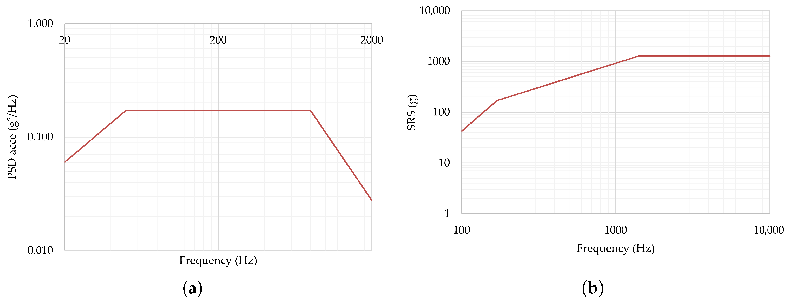
Figure 15. Qualification vibration level profiles for all axes: (a) random vibration; (b) shock response spectrum.

The corresponding Factors of Safety (FOSs) are summarised based on the “Factors of Safety” defined in [22]. These factors are then used to compute the Margin Of Safety (MOS), as shown in Equations (19) and (20), using the von Mises stress ${\sigma }_{\mathrm{v}.\mathrm{m}}$ obtained from the FEM simulations. The terms ${\mathrm{FOS}}_Y$ and ${\mathrm{FOS}}_U$ denote the yield and ultimate Factors of Safety, respectively.

The load factor $K_{\mathrm{LD}}$ represents an additional load amplification factor applied to account for uncertainties in load definition and modelling assumptions, following ECSS recommendations. In this work, a value of $K_{\mathrm{LD}}=1.2$ was adopted. The corresponding safety factors are ${\mathrm{FOS}}_Y=1.1$ and ${\mathrm{FOS}}_U=1.25$, which are used in the MOS evaluation.

$${\mathrm{MOS}}_{\mathrm{yield}}={\displaystyle \frac{{\sigma }_{\mathrm{yield}}}{{\sigma }_{\mathrm{v}.\mathrm{m}}{\mathrm{FOS}}_Y{K}_{\mathrm{LD}}}}-1$$

(19)

$${\mathrm{MOS}}_{\mathrm{ultimate}}={\displaystyle \frac{{\sigma }_{\mathrm{ultimate}}}{{\sigma }_{\mathrm{v}.\mathrm{m}}{\mathrm{FOS}}_U{K}_{\mathrm{LD}}}}-1$$

(20)

In addition, Table 4 summarizes the lumped masses used in the FEM to represent non-structural components such as optical elements and electronic equipment. These masses were implemented using CONM2 elements and connected to the structural mesh through rigid links to ensure proper inertia distribution without over-refining the mesh.

Table 4. Lumped mass representation of the optical instrument components.

Component	Qty.	Mass (gram)	Model Representation
Lens assembly	1	15.0	Concentrated mass at optical axis (CONM2)
Baffle vanes	3	8.54	Distributed lumped masses along baffle structure
PCB1 (Sensor)	1	5.64	Lumped mass linked to PCB nodes
PCB2 (Processor)	1	8.64	Lumped mass linked to PCB nodes
PCB3 (Output)	1	6.86	Lumped mass linked to PCB nodes
EEE components	–	12.0 (approx.)	Equivalent distributed masses on PCBs
Connector	1	4.26	Lumped mass at interface location

The main areas of interest in the analysis were the structural components, the PCBs, and the radiation lens window, due to their size and functional importance.

Structural Results

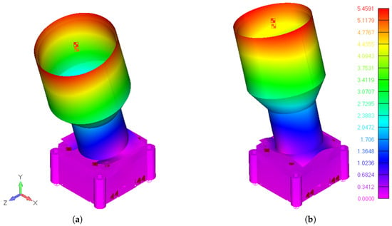
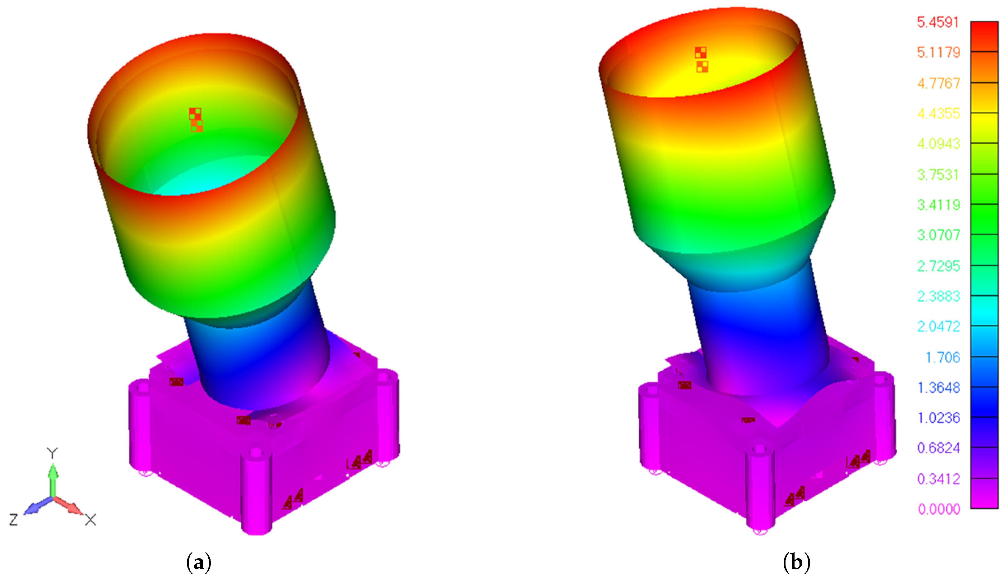
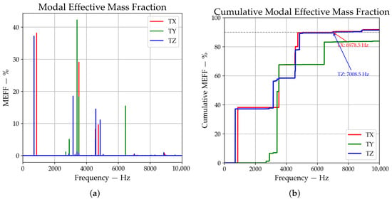
The modal analysis identified the first two mode shapes at 705.3 Hz and 868.1 Hz, corresponding to structural deformation of the baffle.

These are illustrated in Figure 16a,b. The characteristics of the baffle geometry—namely its length and diameter—are clearly associated with these two modes.

Figure 16. First structural mode shapes of the instrument: (a) first mode at 705.3 Hz and (b) second mode at 868.1 Hz.

The remaining resonances start at 2702 Hz and above, where the dominant modal shapes shift to other components such as the PCBs, enclosure, lid, and radiation lens. This is confirmed by the Modal Effective Mass (MEM) results shown in Figure 17a,b, where the Modal Effective Mass Fraction (MEFF) and its cumulative distribution highlight distinct resonance zones: the baffle modes around 705.3 Hz and 868.1 Hz and contributions from smaller elements such as the PCBs and enclosure above 2702 Hz.

Figure 17. Modal Effective Mass Fraction Results: (a) MEFF; (b) cumulative MEFF.

For the dynamic analyses (random vibration and shock response), the modal basis was extended to cover the frequency range up to 10 kHz, ensuring that all dynamically relevant modes contributing to the response were included. This is consistent with the qualification spectra, where random vibration is typically limited to 2 kHz, while shock response can excite higher-frequency modes.

A structural damping ratio of 5% of critical damping was assumed for both random vibration and shock response analyses, which is a typical value for aluminium structures with assembled interfaces. This parameter governs the dynamic amplification of the response and, consequently, the resulting stress levels under broadband and transient excitation. According to the Askenazi technical reference [23], the intrinsic damping of metals in the elastic range is generally very low ($\xi <1\%$), whereas assembled metallic structures exhibit significantly higher effective damping due to interface-related dissipation mechanisms. In particular, structures with mechanical joints typically present damping ratios in the range of $3\%$ to $7\%$, driven by frictional effects, micro-slip, and local nonlinearities at contact interfaces. In addition, the European Cooperation for Space Standardization (ECSS) framework recommends the use of equivalent viscous damping ratios to represent the global structural dissipation in dynamic analyses, with typical engineering values ranging from $2\%$ to $5\%$, depending on the structural configuration and level of assembly [24]. Therefore, the adoption of $\xi =5\%$ is considered representative and slightly conservative for the present configuration, ensuring that interface-driven damping contributions are adequately captured without underestimating the structural response. Although damping is inherently mode-dependent and may vary with frequency and excitation level, the use of a constant equivalent damping ratio remains standard practice for qualification-level analyses.

Both modes shown in Figure 16 are dominated by deformation of the baffle, confirming its significant influence on the dynamic behaviour of the system. The selected modal range, together with the adopted damping assumption, ensures that the dynamic response is accurately captured for both random and shock load cases, and that the resulting stress state reflects realistic amplification effects across the full excitation spectrum.

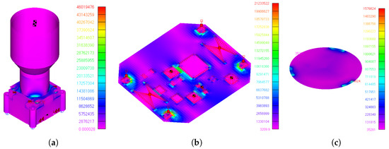
Importantly, for structural tests such as sinusoidal and random vibration, the most critical resonance frequencies are those associated with the baffle. This is because sinusoidal vibration tests typically do not exceed 120 Hz, and random vibration tests are generally limited to 2000 Hz. Therefore, if the first natural frequency is above 120 Hz, sinusoidal vibration tests may be waived, as resonance amplification is not expected—making a quasi-static acceleration analysis sufficient. However, random vibration and shock analyses and tests remain necessary. Random vibrations can excite frequencies up to 2000 Hz, and shock tests may extend to 10,000 Hz, both of which can introduce nonlinear amplification effects. These require dedicated simulation and corresponding qualification testing to ensure structural integrity. Figure 18 shows that random vibration and shock response are the main sources of high mechanical stress on the components. For the structural element, primarily made of Aluminium 6061, the highest stress occurs under random vibration along the Z-axis. For the PCB, the maximum stress is induced by the shock response along the Y-axis, while for the radiation lens window, the peak stress is observed under shock response along the Z-axis.

Figure 18. Maximum von Mises stress distribution under critical loading conditions: (a) structural components under random vibration (Z-axis), (b) PCB under shock response (Y-axis), and (c) radiation lens window under shock response (Z-axis).

Although a quasi-static load case was considered in the design (up to 60 g, with 3$\sigma$), its contribution to the overall stress envelope is lower than that of the dynamic loading cases (random vibration and shock response).

This is further confirmed by the stress values summarized in Table 5, where the maximum stresses are governed by random vibration and shock responses rather than quasi-static loading.

Table 5. Summary of von Mises stress and Margins of Safety for the instrument components.

Part	Material	Max Stress ${\mathit{\sigma }}_{\mathbf{v}.\mathbf{m}}$ (MPa)	MOSyield	MOSultimate
Structural	Al 6061	138.0	0.51	0.50
PCBs	FR4	21.2	6.14	5.28
Radiation Lens	N-BK7	1.6	22.02	19.26

${\mathrm{MOS}}_{\mathrm{yield}}$ and ${\mathrm{MOS}}_{\mathrm{ultimate}}$ are positive for all parts, with the lowest value of 0.5 on the structural aluminium parts, as shown in Table 5.

It is important to highlight that the optical, thermal, and structural performances of the system are strongly coupled through the baffle design. While the baffle plays a critical role in achieving low stray-light levels and improving the SNR of 5 dB, its geometry and surface properties significantly influence both thermal and structural behaviour. From a thermal perspective, the large exposed surface of the baffle directly affects the absorption of solar and Earth albedo radiation, contributing to the overall thermal balance of the instrument. From a structural standpoint, the baffle represents a relatively large and extended component, influencing the mass distribution and defining the first vibration modes around 705.3 Hz, as observed in the modal analysis. These results highlight an inherent design trade-off: optimizing the baffle for optical performance may negatively impact thermal and structural responses, and vice versa. Therefore, a balanced multidisciplinary design approach is required to ensure overall system performance.

6. Conclusions

The main objective of this work was to design, model, and validate a miniaturized dual-purpose instrument capable of functioning both as a star tracker and a space-debris detection camera. This was achieved through the development of detailed numerical models for the optical, thermal, and structural domains—namely an optical ray-tracing model, a lumped-parameter thermal model, and a structural finite-element model—followed by a comprehensive performance assessment to determine the feasibility of the concept.

Beyond the development of a specific instrument, this work provides relevant contributions to the current state of the art. In particular, it presents, to the authors’ knowledge, the first compact dual-purpose star tracker and debris detection camera validated through a consistent multidisciplinary framework, where optical, thermal, and structural performances are analysed in a unified manner. Furthermore, the study highlights the strong coupling between baffle design and system-level behaviour, explicitly demonstrating the trade-off between stray-light suppression (and resulting SNR), thermal balance driven by thermo-optical properties, and structural response influenced by geometry and mass distribution.

The study yielded several key findings. In terms of optical performance, the instrument demonstrated effective stray-light suppression, favourable Point Source Transmittance (PST) characteristics, and the capability to achieve the required signal-to-noise ratio (SNR) levels for star and debris detection, with sensitivity of up to approximately magnitude 5.8.

Regarding the thermal performance, the system maintained acceptable margins across both hot and cold cases, with only minor deviations. In particular, the image sensor exceeded its operational limit by approximately +1.1 °C under worst-case hot conditions. Overall, these results indicate robust thermal behaviour, even under direct solar exposure. This minor temperature exceedance is driven by the combined effect of external thermal loads (solar and Earth albedo radiation) and internal heat dissipation from the electronic components. Future design iterations will consider optimized surface treatments (e.g., high-emissivity coatings, second surface mirrors, or MLI) together with improved heat dissipation paths to ensure compliance with operational limits.

From a structural perspective, the camera demonstrated sufficient stiffness and strength under quasi-static, vibration, and shock loading, with safety margins above unity and first natural frequencies well above typical qualification thresholds.

This development confirmed several achievements:

1.

A compact and lightweight design (approximately 172 g with dimensions of 105 × 52 × 52 mm) compatible with small-satellite constraints;

2.

A validated assembly and modelling approach ensuring optical alignment, thermal performance, and mechanical integrity;

3.

The demonstration of a dual-purpose optical instrument combining star tracking and debris detection capabilities within a single compact architecture.

Nevertheless, some limitations remain. In particular, the thermal model has not yet been correlated with experimental data, and the slight hot-case temperature exceedance requires validation through testing.

Future work will focus on experimental validation and qualification of the proposed instrument, including thermal-vacuum and vibration testing, as well as dedicated stray-light laboratory measurements under controlled illumination conditions Particular attention will be given to the validation of the signal-to-noise ratio (SNR) model used as a performance indicator for stray-light suppression, ensuring consistency between numerical predictions and experimental results. Ultimately, in-orbit demonstration will enable full correlation between laboratory, simulation, and operational data.

The results also demonstrate that the optical, thermal, and structural performances of the instrument are intrinsically coupled, with the baffle acting as the primary element linking these domains. While it is essential for achieving the required stray-light suppression, its geometry and thermo-optical properties directly influence the thermal balance, and its mass distribution affects the structural dynamic behaviour. This interplay highlights a fundamental design trade-off, reinforcing the need for a multidisciplinary design approach.

Beyond the design and validation of a specific instrument, this work provides several original contributions with respect to the current state of the art. First, it presents, to the authors’ knowledge, the first compact dual-purpose optical instrument that integrates star tracking and space debris detection capabilities within a single architecture, validated through a consistent optical, thermal, and structural modelling framework.

Second, the study explicitly demonstrates the strong coupling between baffle design and system-level performance, highlighting a key trade-off between stray-light suppression (and resulting SNR), thermal behaviour driven by surface properties and radiative balance, and structural dynamics influenced by mass distribution and geometry. This multidisciplinary interaction is often treated separately in the literature and is here addressed in a unified manner.

Finally, the work contributes a practical design and modelling methodology for small satellite optical payloads, combining ray-tracing-based stray-light analysis, lumped-parameter thermal modelling, and finite element structural analysis within a coherent workflow. This approach enables the identification of optimal design compromises at an early stage and can be directly applied to future compact, multifunctional space instruments.

Overall, this work establishes a coherent design and validation framework for compact multifunctional optical payloads, contributing to the development of next-generation small-satellite instruments for navigation and space situational awareness.

References

- Liebe, C.C. Star trackers for attitude determination. IEEE Aerosp. Electron. Syst. Mag. 1995, 10, 10–16. [Google Scholar] [CrossRef] [Scilit]
- Sang, P.; Liu, W.; Cao, Y.; Xue, H.; Li, B. Research on precise attitude measurement technology for satellite extension booms based on the star tracker. Sensors 2024, 24, 6671. [Google Scholar] [CrossRef] [Scilit] [PubMed]
- Liu, X.; Xing, F.; Fan, S.; You, Z. A compressed and high-accuracy star tracker with on-orbit deployable baffle for remote sensing cubesats. Remote Sens. 2021, 13, 2503. [Google Scholar] [CrossRef] [Scilit]
- Filho, J.; Gordo, P.; Peixinho, N.; Melicio, R.; Gafeira, R. Payload camera breadboard for space surveillance—Part I: Breadboard design and implementation. Appl. Sci. 2023, 13, 3682. [Google Scholar] [CrossRef] [Scilit]
- Filho, J.; Gordo, P.; Peixinho, N.; Melicio, R.; Gafeira, R. Space surveillance payload camera breadboard: Star tracking and debris detection algorithms. Adv. Space Res. 2023, 72, 4215–4228. [Google Scholar] [CrossRef] [Scilit]
- Filho, J.; Gordo, P.; Peixinho, N.; Gafeira, R.; Melicio, R.; Silva, A. Satellite star tracker breadboard with space debris detection capability for LEO. J. Phys. Conf. Ser. 2023, 2526, 012119. [Google Scholar] [CrossRef] [Scilit]
- Brown, J.; Stubis, K.; Cahoy, K. TETRA: Star identification with hash tables. In Proceedings of the 31st Annual AIAA/USU Conference on Small Satellites, Logan, UT, USA, 5–10 August 2017; Utah State University: Logan, UT, USA, 2017; pp. 1–12. [Google Scholar]
- Kim, D.-W. ASTRiDE: Automated Streak Detection for Astronomical Images. Available online: https://github.com/dwkim78/ASTRiDE (accessed on 15 February 2026).
- Arribas, B.N.; Maia, J.G.; Castanheira, J.P.; Filho, J.; Melicio, R.; Onderwater, H.; Gordo, P.; Duarte, R.P.; Silva, A.R.R. Dual-purpose star tracker and space debris detector: Miniature instrument for small satellites. J. Sens. Actuator Netw. 2025, 14, 75. [Google Scholar] [CrossRef] [Scilit]
- Liu, S.; Zhang, J.; Sun, G.; Zhang, G.; Chen, S.; Chen, J. Research on evaluation index of stray light suppression ability of star sensor based on signal-to-noise ratio. Opt. Commun. 2023, 530, 129175. [Google Scholar] [CrossRef] [Scilit]
- Sinclair, D.; Enright, J.; Dzamba, T.; Sears, T.M.C. Custom optics vs. modified COTS for small spacecraft: The build vs. rebuild decision or A Case Study in Applied Hubris. In Proceedings of the AIAA/USU Conference on Small Satellites, Logan, UT, USA, 8–13 August 2015; pp. 1–11. [Google Scholar]
- Sinclair, D.; Enright, J.; Dzamba, T.; Sears, T.M.C. Custom optics vs. modified COTS for small spacecraft: The build vs. rebuild decision. In Proceedings of the AIAA/USU Conference on Small Satellites, Logan, UT, USA, 8–13 August 2015; pp. 1–11. [Google Scholar]
- Asadnezhad, M.; Eslamimajd, A.; Hajghassem, H. Optical system design of star sensor and stray light analysis. J. Eur. Opt. Soc. Rapid Publ. 2018, 14, 9. [Google Scholar]
- Lee, Y.S.; Kim, Y.H.; Yi, Y.; Kim, J. A baffle design for an airglow photometer on board the Korea Sounding Rocket-III. J. Korean Astron. Soc. 2000, 33, 165–172. [Google Scholar]
- ECSS-E-HB-31-03A; Space Engineering—Thermal Analysis Handbook. ESA Requirements and Standards Division: Noordwijk, The Netherlands, 2016.
- Synopsis Planet, Star Tracker and Space Debris Monitor. Available online: https://www.linkedin.com/posts/synopsis-planet_newspace-prr-madeinportugal-activity-7313155551457124352-tLKh (accessed on 20 August 2025).
- Shi, R.; Zhou, J.; Ji, Y.; Shen, W. Stray light analysis and baffle design of remote sensing camera for microsatellite. In Proceedings of 2009 International Conference on Optical Instruments and Technology: Optical Systems and Modern Optoelectronic Instruments, Shanghai, China, 4 November 2009; SPIE: Bellingham, WA, USA, 2009; p. 75060T. [Google Scholar]
- Wang, G.; Xing, F.; Wei, M.; You, Z. Rapid optimization method of the strong stray light elimination for extremely weak light signal detection. Opt. Express 2017, 25, 26175. [Google Scholar] [CrossRef] [Scilit] [PubMed]
- Plesseria, J.Y.; Mazy, E.; Defise, J.M.; Rochus, P.; Lemmens, E.; Vrancken, D. Optical and Mechanical Design of a Straylight Rejection Baffle for COROT. pp. 1–10. Available online: https://orbi.uliege.be/bitstream/2268/21190/1/COROT_spie_2003.pdf (accessed on 15 February 2026).
- Peterson, G.L. Stray light test station for measuring point source transmission and thermal background of visible and infrared sensors. In Proceedings of Optical System Contamination: Effects, Measurements, and Control, San Diego, CA, USA, 28 August 2008; SPIE: Bellingham, WA, USA, 2008; p. 70690M. [Google Scholar]
- ECSS-E-HB-31-01 Part 4A; Space Engineering—Thermal Design Handbook: Conductive Heat Transfer. ESA Requirements and Standards Division: Noordwijk, The Netherlands, 2011.
- ECSS-E-ST-32-10C; Space Engineering—Structural Factors of Safety for Spaceflight Hardware. ESA Requirements and Standards Division: Noordwijk, The Netherlands, 2009.
- Askenazi, A.; Adams, V. Building Better Products with Finite Element Analysis; OnWord Press: Santa Fe, NM, USA, 1998; Table 18.2. [Google Scholar]
- ECSS-E-HB-32-26A; Space Engineering—Spacecraft Mechanical Loads Analysis Handbook. ESA Requirements and Standards Division: Noordwijk, The Netherlands, 2013.
- Arcsec. Twinkle. Available online: https://www.arcsec.space/twinkle/ (accessed on 15 February 2026).
- Rocket Lab. ST-16RT2. Available online: https://rocketlabcorp.com/assets/Uploads/ST-16RT2-Datasheet-v4.1.pdf (accessed on 15 February 2026).
- Solar MEMS. STNS. Available online: https://www.solar-mems.com/wp-content/uploads/2024/01/STNS.pdf (accessed on 15 February 2026).
- Arcsec. Sagitta. Available online: https://www.arcsec.space/sagitta/ (accessed on 15 February 2026).
- AAC Clyde Space. ST400. Available online: https://www.aac-clyde.space/what-we-do/space-products-components/adcs/st400 (accessed on 15 February 2026).
- Blue Canyon Technologies. Nano Star Trackers. Available online: https://www.bluecanyontech.com/components/nano-star-trackers/ (accessed on 15 February 2026).
- Kairo Space. KSST-01 Star Tracker. Available online: https://www.kairo.space/products/ksst-01-star-tracker (accessed on 15 February 2026).
- Sodern. Auriga-CP. Available online: https://api.sodern.com/uploads/AURIGA_CP_bb09019ea5.pdf (accessed on 15 February 2026).
- Sodern. Auriga-SA. Available online: https://api.sodern.com/uploads/AURIGA_SA_21e79319c1.pdf (accessed on 15 February 2026).
- Space Inventor. STR-P4. Available online: https://space-inventor.com/equipment/startracker (accessed on 15 February 2026).
- Jena-Optronik. Astro-CL. Available online: https://jena-optronik.de/products/star-sensors/astro-cl.html (accessed on 15 February 2026).
- Arcsec. Scorpio. Available online: https://www.arcsec.space/scorpio/ (accessed on 15 February 2026).
- Space Micro. Star-250. Available online: https://www.satnow.com/products/star-trackers/space-micro/37-1219-star-250 (accessed on 15 February 2026).
- Sodern. Horus. Available online: https://api.sodern.com/uploads/HORUS_4870fe0b49.pdf (accessed on 15 February 2026).
- SatCatalog. Star-200M. Available online: https://www.satcatalog.com/component/star-200m/ (accessed on 15 February 2026).
- Jena-Optronik. Astro-APS. Available online: https://jena-optronik.de/products/star-sensors/astro-aps.html (accessed on 15 February 2026).
- Sodern. Hydra-CP. Available online: https://api.sodern.com/uploads/VISEUR_HP_8_PAGE_2b387a8966.pdf (accessed on 15 February 2026).
- Jena-Optronik. Astro-XP. Available online: https://www.jena-optronik.de/products/star-sensors/astro-xp.html (accessed on 15 February 2026).
Disclaimer/Publisher’s Note: The statements, opinions and data contained in all publications are solely those of the individual author(s) and contributor(s) and not of MDPI and/or the editor(s). MDPI and/or the editor(s) disclaim responsibility for any injury to people or property resulting from any ideas, methods, instructions or products referred to in the content. |
© 2026 by the authors. Licensee MDPI, Basel, Switzerland. This article is an open access article distributed under the terms and conditions of the Creative Commons Attribution (CC BY) license.