


Abstract
During the preliminary design of flight vehicles, i.e., missiles or guided rockets, propulsion system performance serves as a critical determinant of both maximum range and terminal velocity. However, complex grain configurations in solid rocket motors (SRMs) typically require geometric modeling software to obtain burning surface area, which severely constrains efficiency. To address this challenge, this study presents a neural network-enhanced rapid performance prediction and matching optimization framework for solid rocket motors (NN-SRM). In NN-SRM, neural networks are employed to simulate the evolution of key parameters during grain combustion, including burning surface area, grain volume, and moment of inertia. The zero-dimensional internal ballistics equations coupled with one-dimensional steady isentropic flow relations are incorporated into the framework to rapidly obtain thrust curves. A discrete–continuous mixed differential evolution algorithm is further employed to identify the optimal grain configuration that satisfies specific thrust requirements. Results demonstrate that, as for cylindrical, star, and finocyl grains, the neural network achieves R2 exceeding 0.95. Finally, thrust matching optimization is conducted on three grains and achieves promising thrust solutions for the conditions of large thrust with short time and small thrust with long time, which demonstrates the effectiveness and practicality of the constructed NN-SRM.
1. Introduction
Solid rocket motors (SRMs) are widely employed in various missiles, spacecraft, and launch vehicles due to their simple structure, long-term propellant storability, high reliability, and ease of operation and maintenance [1]. During the preliminary design of the flight vehicle, the SRM internal ballistics requires meticulous design and optimization [2,3], since it is critical to maximum range and terminal velocity. Traditionally, the design and performance prediction of SRMs with complex grain configurations heavily rely on the geometric modeling software, which is computationally intensive and simultaneously increases the design complexity [4].
With the emergence of machine learning technology, novel methodologies, especially various neural networks (NNs), have been applied in SRM modeling and performance prediction [5]. As for thrust prediction, Zhang et al. [6] have employed a deep neural network architecture based on ConvNeXt to extract and learn advanced features of the thrust data. The results have demonstrated that the architecture is highly suitable for thrust time sequence prediction. Lee et al. [7] have conducted a comprehensive investigation of several NNs approximating performance on the grain burn back, including deep neural networks, recurrent neural networks, long short-term memory (LSTM), bidirectional LSTM, gated recurrent units (GRU), and GRUs with fully connected layers models. Beyond thrust prediction, the neural networks have also been successfully applied to defect diagnosis of solid rockets [8,9]. For instance, Korompili et al. [8] have developed a deep learning-based structural health monitoring system for solid rocket motors. Strain sensors and neural networks are combined to detect and quantify internal defects, e.g., bore cracks and delamination. Similarly, in Ref. [9], a deep convolutional neural network architecture is investigated to assess the defect scales of SRM, considering a bore crack and a delamination. According to the aforementioned research, it should be noted that various NNs [7,10,11] hold a promising potential for SRM modeling and other fields of flight vehicles.
Furthermore, an overview research conducted by Geisler et al. [12] has covered various historical and technical aspects of SRM. This review concludes that “though many designs and practices have been proven over the last 60 years, much research remains to be completed toward the optimization of SRM performance”. In engineering practices, the thrust matching optimization is also essential in the preliminary design [13,14,15], as it explores the relationship between the engine’s design parameters and the required thrust curve. For instance, Wu et al. [13] have utilized a two-stage design framework incorporating a sequential field approximate optimization algorithm and level-set method to obtain a thrust curve closely matched to the required one. Li et al. [14] have proposed the concept of modular grain and derived governing equations based on quadratic approximation of burning rules, which can generate rapid and reliable results. Some novel approximate approaches, e.g., surrogates and neural networks, have been initially implemented in thrust matching optimization. Kim et al. [15] have combined an artificial neural network to capture the relationship between the grain geometries and burning area, where an inverse design is conducted to obtain the best grain geometry. In addition, some optimization methods have been utilized to find the best component mass fractions for solid propellant [16].
According to the literature review, it can be found that deep neural networks have received much attention in modeling, designing, and detecting SRMs. However, increasing the number of hidden layers and nodes may constrain the practical engineering application of NNs. In the existing research [15], the layers and neurons are larger than 3 and 128, respectively, which potentially causes the scale of training samples to be unaffordable for engineering design [17,18]. Furthermore, the integration of internal ballistics equations and steady isentropic flow theory with NN architectures is essential to derive comprehensive performance, instead of pure burning area analysis.
To rapidly predict the performance of SRMs and obtain a solution suitable for the requirements, this paper has developed a neural network-enhanced performance rapid prediction and matching optimization framework for SRMs. The geometric models of cylindrical, star, and finocyl grains are constructed to calculate several parameters, including burning area, grain volume, and moment of inertia, under different burnback distances. For each grain type, an NN is trained to reveal the inner relationship between burnback distance and the evolution of the parameters. The thrust matching optimization is then conducted on the NN to rapidly find the best grain configuration that meets the design requirements.
The paper is organized as follows. The neural network-enhanced framework for SRMs is presented in Section 2. In Section 3, the geometric models for three different grains are constructed parametrically. Meanwhile, NNs are trained and validated in this section. Section 4 provides a brief introduction to zero-dimensional internal ballistic equations and one-dimensional steady isentropic flow theory, which are subsequently applied to calculate thrust. Based on the trained NN and thrust simulation model, a thrust matching optimization mathematical model is formulated in Section 5, where a discrete–continuous mixed differential evolution algorithm is employed to explore the best solution. The thrust matching optimization results for two cases are given in Section 6. The conclusions and future work are summarized in Section 7.
2. Neural Network-Enhanced Framework for SRM
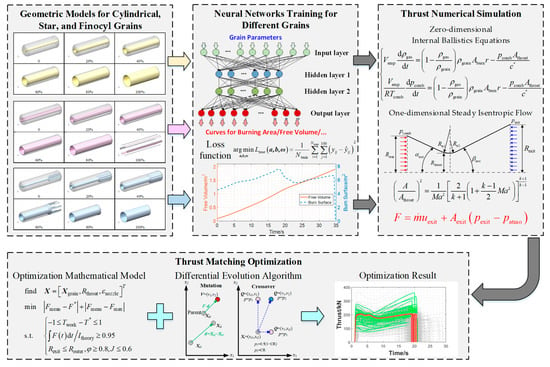
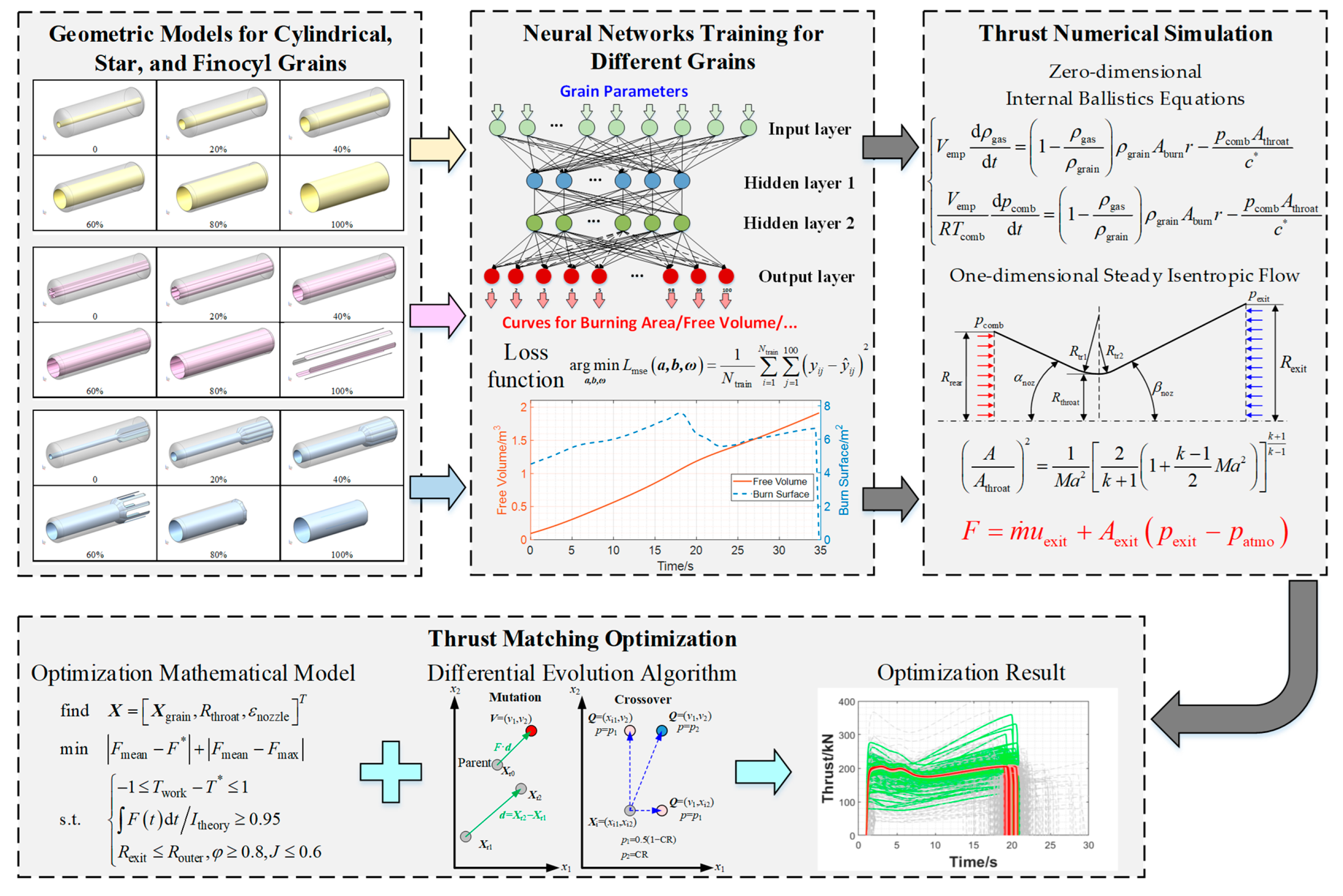
In this paper, a neural network-enhanced framework for SRM (NN-SRM) is developed and illustrated in Figure 1. It can be observed that NN-SRM consists of several modules, namely geometric modeling, neural network training and validation, numerical simulation, and thrust matching optimization. The function of each module is explained as follows.
Figure 1.
Neural network-enhanced framework for SRM.
- (1)
- Geometric modeling module
The geometric modeling module serves as the foundational component of the framework, where three-dimensional configurations of cylindrical, star, and finocyl grains are parametrically constructed. In this module, the grain burnback process is simulated by progressively increasing the offset distance. The variations in burning area, grain volume, and moment of inertia are accordingly computed. Additionally, an optimal Latin hypercube sampling method is combined with this module to generate samples for training and validating neural networks.
- (2)
- Neural network training and validating module
This module is designed to train the neural network, which replaces the computationally expensive evaluations of the geometric model in simulating the grain burnback process. A preprocessing operation is performed to obtain evenly spaced curve outputs and smooth the curves. The layers and neurons of the NN are tuned for each grain according to its dimensionality and complexity. Meanwhile, a Bayesian regularization algorithm is used to optimize the hyperparameters. The approximation accuracy of the trained NN is then evaluated based on the coefficient of determination.
- (3)
- Thrust numerical simulation module
Integrating the trained neural networks with fundamental propulsion physics, this module enables fast and accurate thrust curve computation for SRM. Based on the curves of burning area and free volume, zero-dimensional internal ballistics equations are utilized to describe the dynamics of pressure and density. Furthermore, one-dimensional steady isentropic flow relations are employed to calculate thrust under varying throat diameters and expansion ratios.
- (4)
- Thrust matching optimization module
The thrust matching optimization module aims to identify the optimal grain configurations that most accurately match the desired thrust curve. A corresponding optimization mathematical model is established. Moreover, to handle both continuous and discrete variables, a discrete–continuous mixed differential evolution (DCMDE) algorithm is developed.
3. Grain Modeling and Approximation
This section details the parametric modeling of three grain configurations, i.e., cylindrical, star, and finocyl grains. Based on the generated samples, neural networks are trained and validated, which can rapidly and accurately approximate key parameters such as burning area, free volume, and moment of inertia.
3.1. Grain Geometry Parametric Modeling
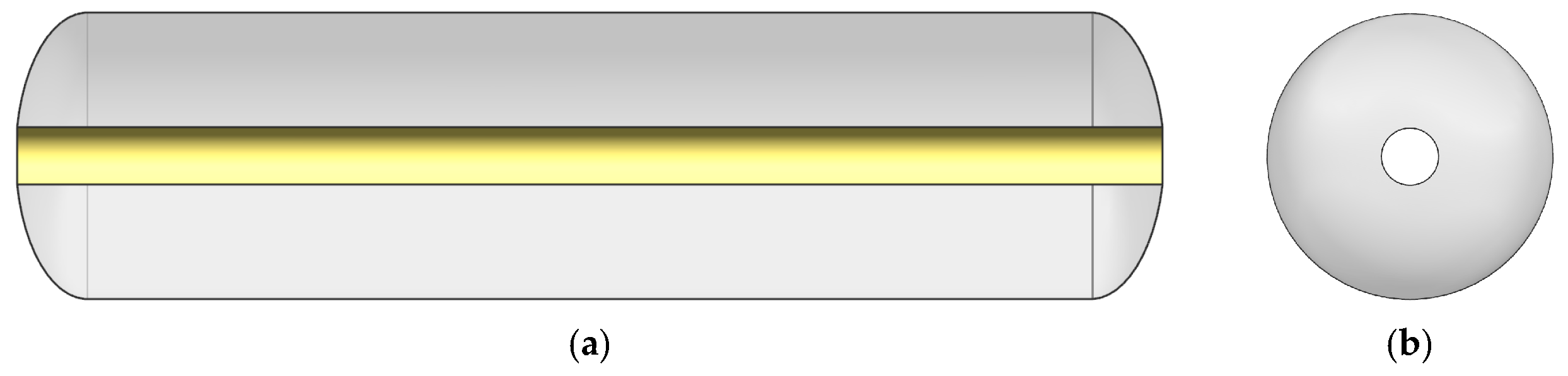
The geometric models of the cylindrical, star, and finocyl grains are shown in Figure 2. These geometric models are uniquely described using 3, 6, and 8 parameters, respectively.
As for the cylindrical grain, the geometry parameters include grain length , grain radius , and port radius . To prevent the generation of unreasonable values for the port radius, the ratio of port radius to grain radius, denoted as , is introduced to calculate , i.e.,
Figure 2.
Geometric models for different grains. (a) Right view of cylindrical grain; (b) front view of cylindrical grain; (c) right view of star grain; (d) front view of star grain; (e) right view of finocyl grain; (f) front view of finocyl grain.
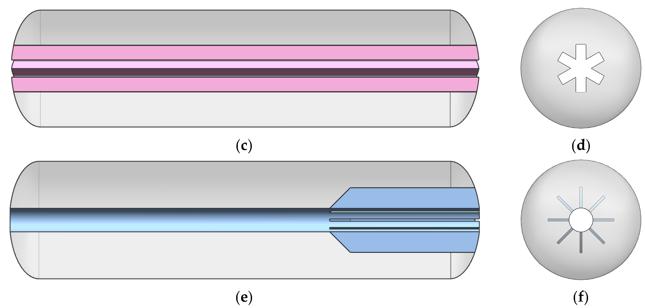
The star grain can be defined by 6 parameters, including grain length , grain radius , characteristic length , star number , star-edge angle , and star angle coefficient . Similarly, the characteristic length is derived as
where is defined as the ratio of characteristic length to grain radius.
The finocyl grain requires 8 parameters to determine its geometry. These parameters are grain length , grain radius , port radius , fin number , decline angle of fin , fin height , tip fin length , and fin thickness . The parameters, including , , , and , are obtained by
where , , and are the ratios of port radius, fin height, and fin thickness to grain radius, respectively; is the ratio of tip fin length to grain length.
To simulate the grain burning process, the burnback distance should be defined to offset the burning surface,
where , , and are the burnback distances for cylindrical, star, and finocyl grains; represents all the integers from 1 to 100.
The detailed information on the parameters for different grains is summarized in Table 1, where the design space for each grain is also provided according to engineering practices. Based on the parameters in Table 1, the geometric models of cylindrical, star, and finocyl grains can be constructed parametrically.
Table 1.
Information on parameters for different grains.
Based on the given design space, an optimal Latin hypercube sampling method [19] is applied to generate sample points. To balance the complexity of the grain geometry and the computational budget, the number of sample points for cylindrical, star, and finocyl grains is set to be 500, 800, and 800, respectively. The responses (e.g., burning area, residual volume, and moment of inertia) of these generated sample points are then calculated by invoking the geometric models. The burnback distance is progressively increased during this process to simulate the burnback procedure at each sample point.
3.2. Neural Network Training and Validation
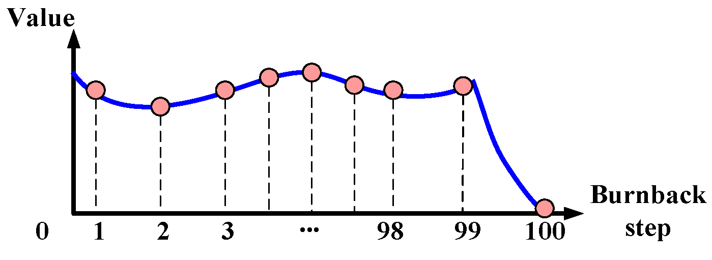
Before training the neural network, the training samples need to be preprocessed. The burning area curve of the sample is divided into 100 equal intervals, as shown in Equation (5), with the step size determined by
where , , and are the burnback step sizes for cylindrical, star, and finocyl grains, respectively. In this way, the burning area curve is transformed into 100 discrete values, which are regarded as the output of the sample. Similarly, the curves of grain volume, residual volume, and moment of inertia are each divided into 100 discrete values for training the neural network, as shown in Figure 3.
Figure 3.
Diagram of curve divided into equal intervals.
During the iterative geometric modeling process with incremental offsets, numerical errors may induce slight oscillations in the curves of various parameters. Therefore, a Savitzky–Golay filtering method is applied to smooth the curves. As for the data sequence where , the Savitzky–Golay filter fit the local data with a polynomial of order , which is formulated as
For each where , a window with size is set to optimize the local polynomial coefficients, i.e.,
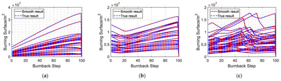
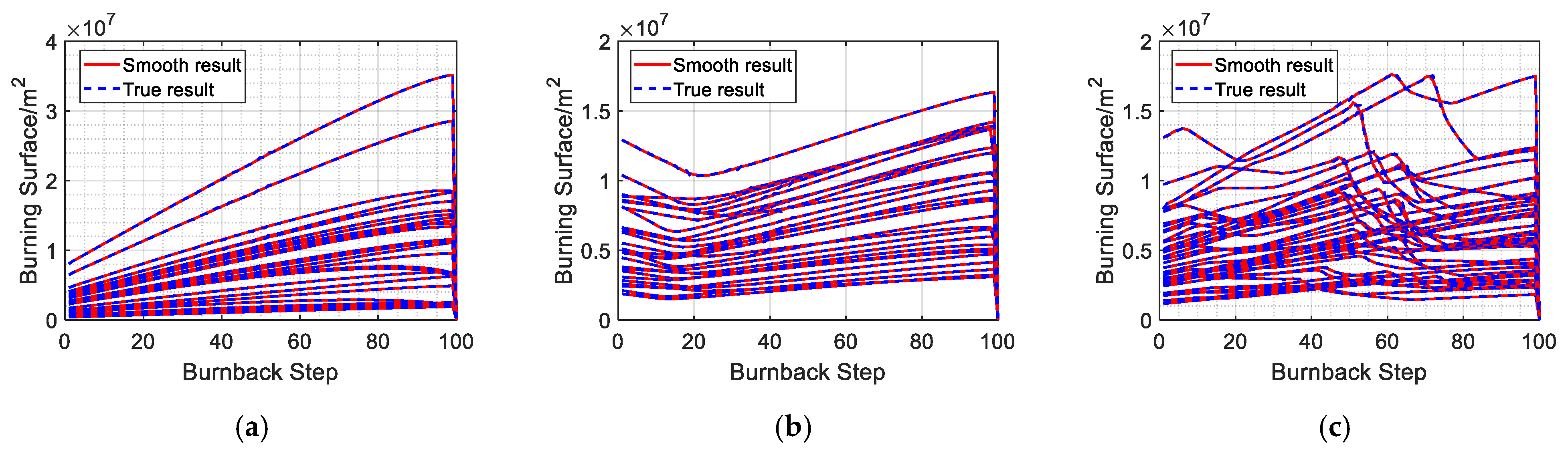
To analysis whether the important features are destroyed, a comparative study is carried out and summarized in Figure 4. It can be found that the filtered results for all the grain are consistent with the true ones, where the physically important features can be retained.
Figure 4.
Comparison of smooth and true results. (a) Cylindrical; (b) star; (c) finocyl.
According to Equations (6) and (7), the oscillations in curves can be smoothed, thereby preventing the trained neural network from learning error patterns.
The sizes of the neural networks for each grain, along with the numbers of training and testing samples, are listed in Table 2. It should be noted that since the finocyl grain has the highest dimensionality of the grain parameters and the most complex burnback behavior, the neural network for this grain employs two hidden layers, while those for other grains use only one.
Table 2.
NN size for each grain.
For each neural network, the activation function of the hidden layer is the hyperbolic tangent function, i.e., Equation (8), and that of the output layer is linear function, i.e., Equation (9).
where , , , and are the hyperparameters of the NNs. To optimize these hyperparameters, a Bayesian regularization algorithm is then employed [20,21], which demonstrates strong resistance to overfitting and promising performance for small sample problems. The loss function can be formulated as
where is the vector consisting of all the hyperparameters; is the weight decay parameter; is the noise precision parameter; and are the error and regularization terms; and are the number of training samples and hyperparameters.
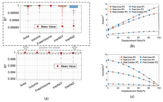
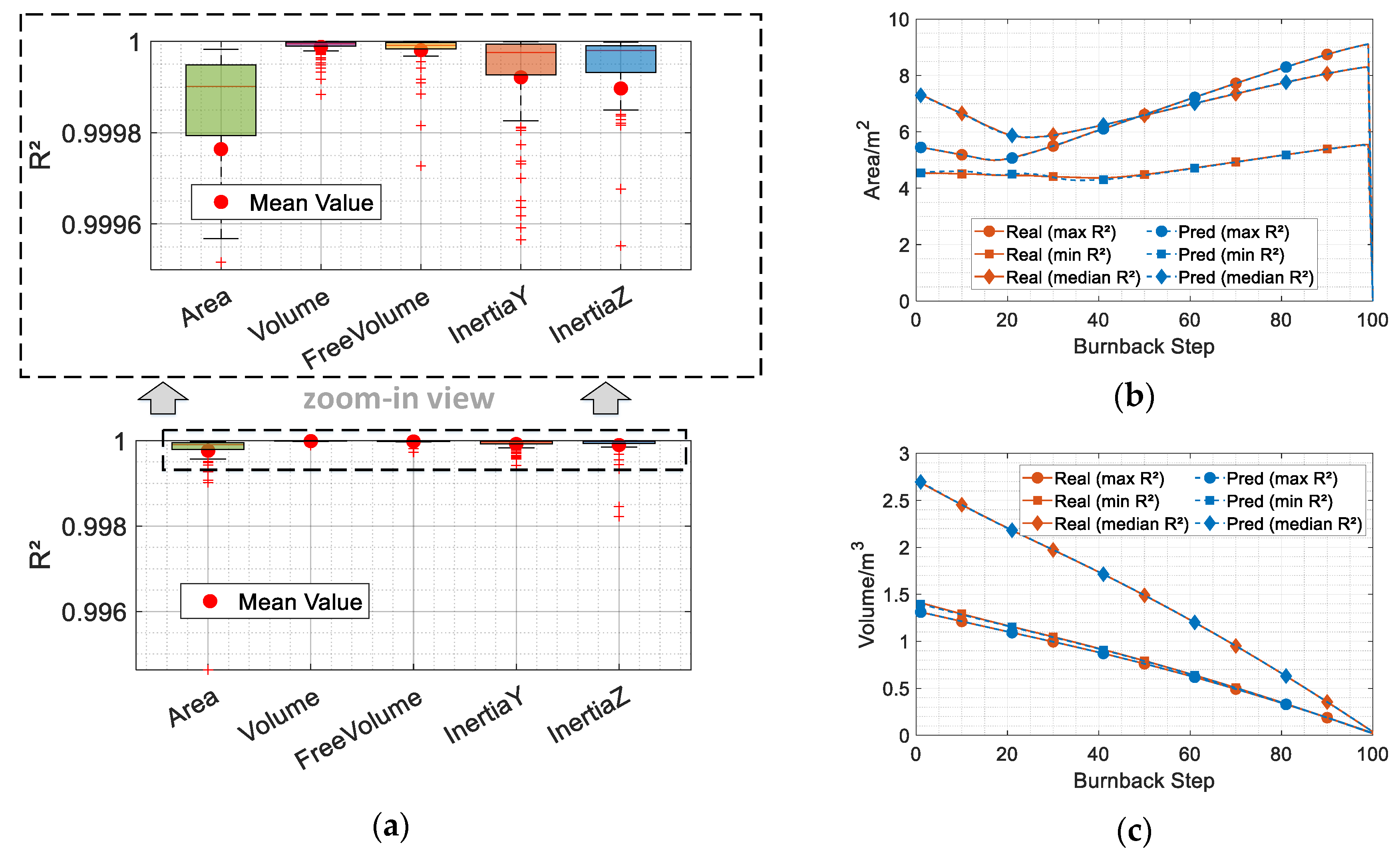
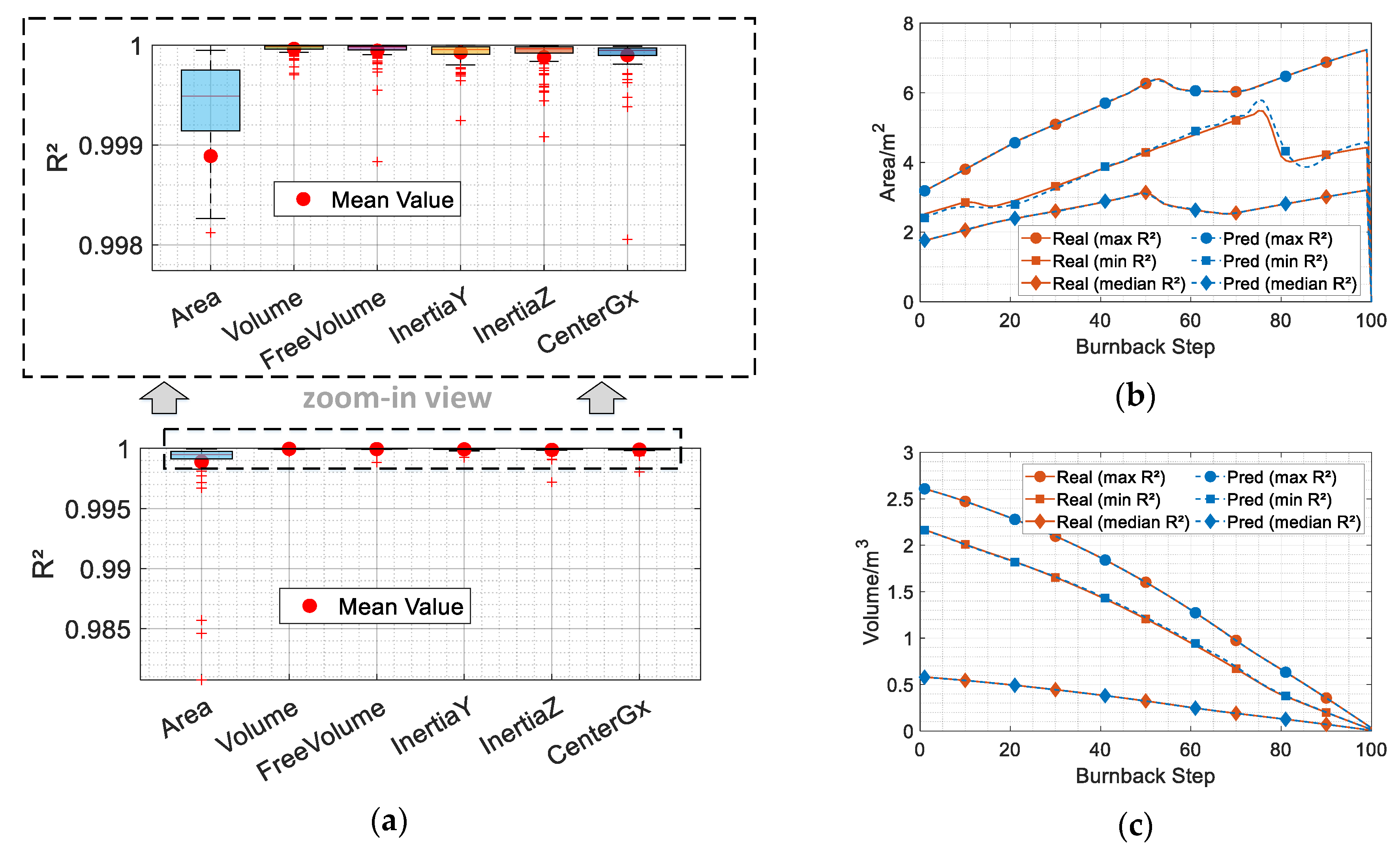
Because the predicted output of the NN consists of multiple components with a broad dynamic range, is adopted as the criterion for evaluating approximation accuracy. The of the th test sample can be expressed as Equation (11). The NN approximation accuracy results for the cylindrical, star, and finocyl grains are illustrated in Figure 5, Figure 6 and Figure 7, respectively.
Figure 5.
Approximation accuracy of NN for cylindrical grain. (a) NN R2; (b) typical area curves; (c) typical grain volume curves.
Figure 6.
Approximation accuracy of NN for Star Grain. (a) NN R2; (b) Typical area curves; (c) typical grain volume curves.
Figure 7.
Approximation accuracy of NN for finocyl grain. (a) NN R2; (b) typical area curves; (c) typical grain volume curves.
As shown in Figure 5b,c, both the burning area and residual volume curves of the cylindrical grain exhibit approximately linear relationships. The configuration parameters of the cylindrical grain are three-dimensional. Consequently, the values of the NN for the area, volume, and inertia all exceed 0.99, with both the mean and median values surpassing 0.999, according to Figure 5a. Furthermore, in Figure 5b,c, it can be observed that the predicted curves with the worst approximation accuracy can still capture the trends of the true curves, thereby verifying the effectiveness of the neural network.
Similarly, as illustrated in Figure 6b, the burning area curve of the star grain changes relatively gently, while the grain configuration parameters are six-dimensional. The values of the one-layer NN for both area and volume exceed 0.99. From Figure 6a, it can be found that there is a slight discrepancy between the predicted curve with the worst accuracy and the corresponding true curve within the first 40 burnback steps. This is because when the burnback step is less than 40, the star-shaped edges gradually vanish, causing the burning area to transition from a decreasing to an increasing trend. This shift increases the nonlinearity of the burning area curve and brings certain errors to the neural network approximation.
Different from the cylindrical and star grains, the NN for the finocyl grain should additionally approximate the location of the center of gravity, which dynamically shifts during the burnback process. Due to the complexity of the burning area curve, the value of the finocyl grain’s area decreases compared to that of the other grains. Nevertheless, the area, residual volume, free volume, inertia, and location of the center of gravity are accurately approximated by the two-layer NN, with all values exceeding 0.98, as illustrated in Figure 7a. From Figure 7b, it can be noted that the area curves vary greatly according to the configuration parameters. However, the predicted curve with the minimum value still accurately captures the overall trend of the true curve.
In conclusion, the neural networks can accurately approximate the key performance parameters of the three grain types, including burning area, residual volume, free volume, and inertia.
4. Thrust Numerical Simulation
In this section, zero-dimensional internal ballistics equations and one-dimensional steady isentropic flow theory are employed to work with the trained neural network to calculate thrust.
4.1. Zero-Dimensional Internal Ballistic Equations
The zero-dimensional internal ballistics equation for the SRM is derived from the principle of mass conservation and the ideal gas state equation [13]. It should be noted that the zero-dimensional internal ballistic model assumes spatially uniform pressure and ignores complex vortical flows within the combustion channel. Such flows influence the pressure field and burning rate. Since the main efforts are put on the neural network-assisted thrust calculation, this phenomenon is ignored. The internal ballistic equations can be formulated as
where and are the free volume and burning area, respectively; and are the gas density and combustion pressure; is the grain density; is the characteristic velocity, calculated by
where is the gas constant; is the working temperature; is a value connected to the specific heat ratio ; and are the universal gas constant and the molar mass. Although a constant specific heat ratio introduces a certain error, this paper focuses on the comparative trends of thrust, pressure, and burning surface area among different grain configurations, where the error due to can be acceptable. The error of the constant specific heat ratio is a limitation of the current constructed model.
The burning rate is expressed as a function of the burning rate coefficient and pressure exponent , i.e.,
The parameters of internal ballistics are listed in Table 3. Based on the zero-dimensional internal ballistics equation, the temporal variation in gas density , pressure , and working time can be determined.
Table 3.
Parameters of internal ballistics.
4.2. One-Dimensional Steady Isentropic Flow
The working medium in the nozzle can be simplified as one-dimensional steady isentropic flow, when the following conditions are satisfied
where is the gas mass flow rate; is the cross-section area of a certain point (denoted as ) in the nozzle; , , and are the gas density, velocity, and pressure at , respectively; is the specific enthalpy of the gas. According to Equations (16)–(19) and the first law of thermodynamics, the nozzle exit velocity can be obtained by
where is the nozzle exit pressure, determined from its relationship with nozzle expansion ratio , as shown in the following equation.
The mass rate is derived from
Thus, the thrust can be calculated by
4.3. Example of Different Grains Configurations
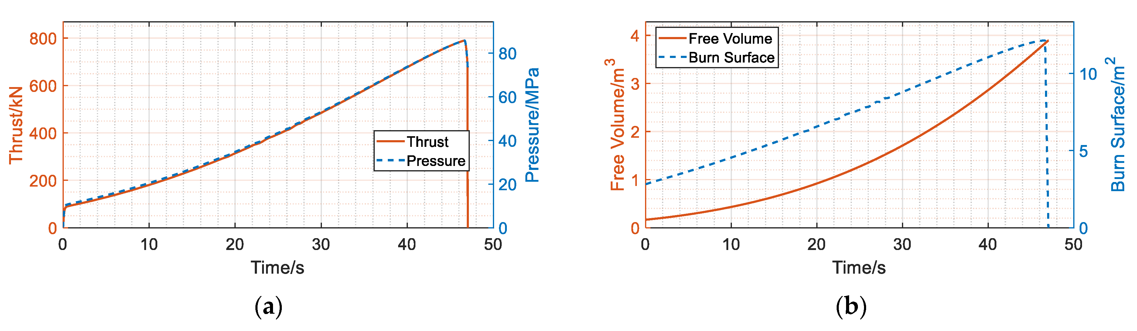
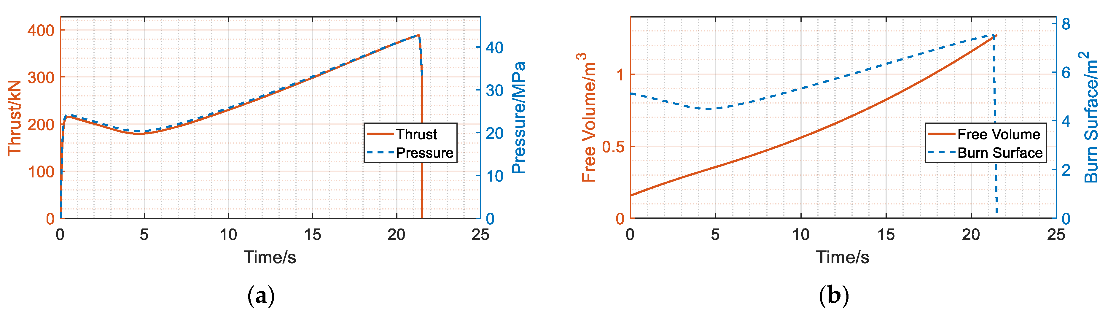
The thrust curves for different grain configurations are presented in Figure 8, Figure 9 and Figure 10. According to Figure 8, the pressure and thrust of the cylindrical grain exhibit an increasing trend, consistent with the evolution of the burning surface area over time. The trends of the pressure and thrust are consistent, since the nozzle throat ablation is not considered in this paper. From Figure 8b, the increasing rate of free volume rises with the burning surface area, thereby further validating the rationality of the established model.
Figure 8.
NN-enhanced performance prediction for cylindrical grain. (a) Thrust and pressure; (b) free volume and burn surface.
Figure 9.
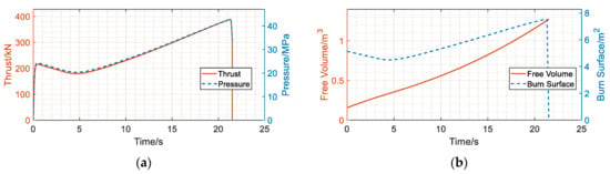
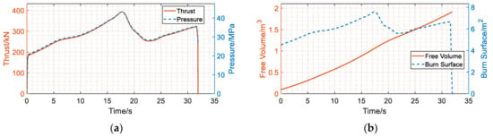
NN-enhanced performance prediction for star grain. (a) Thrust and pressure; (b) free volume and burn surface.
Figure 10.
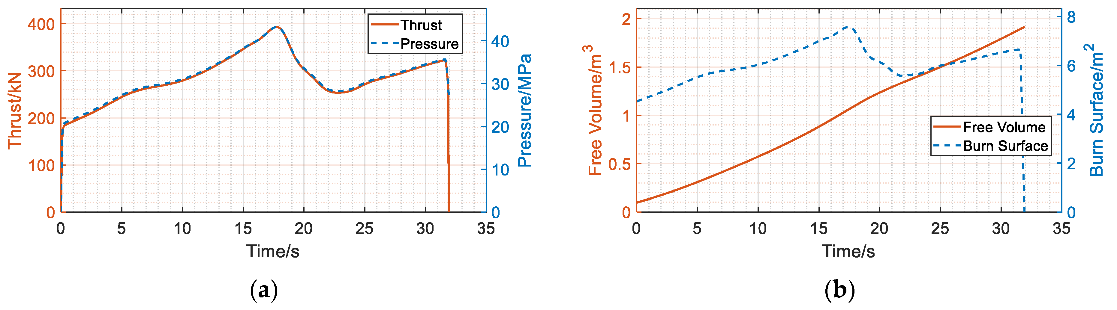
NN-enhanced performance prediction for finocyl grain. (a) Thrust and pressure; (b) free volume and burn surface.
As for the star grain configuration, the thrust, pressure, and burning surface area curves in Figure 9 exhibit a trend of initial decrease followed by an increase. Additionally, the thrust and pressure curves of the finocyl grain exhibit a similar relationship, as illustrated in Figure 10. It can be concluded that different grain configurations yield distinct thrust curves, which affect the trajectory characteristics of the flight vehicle. It is crucial to conduct thrust matching optimization based on different grain configurations.
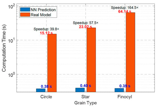
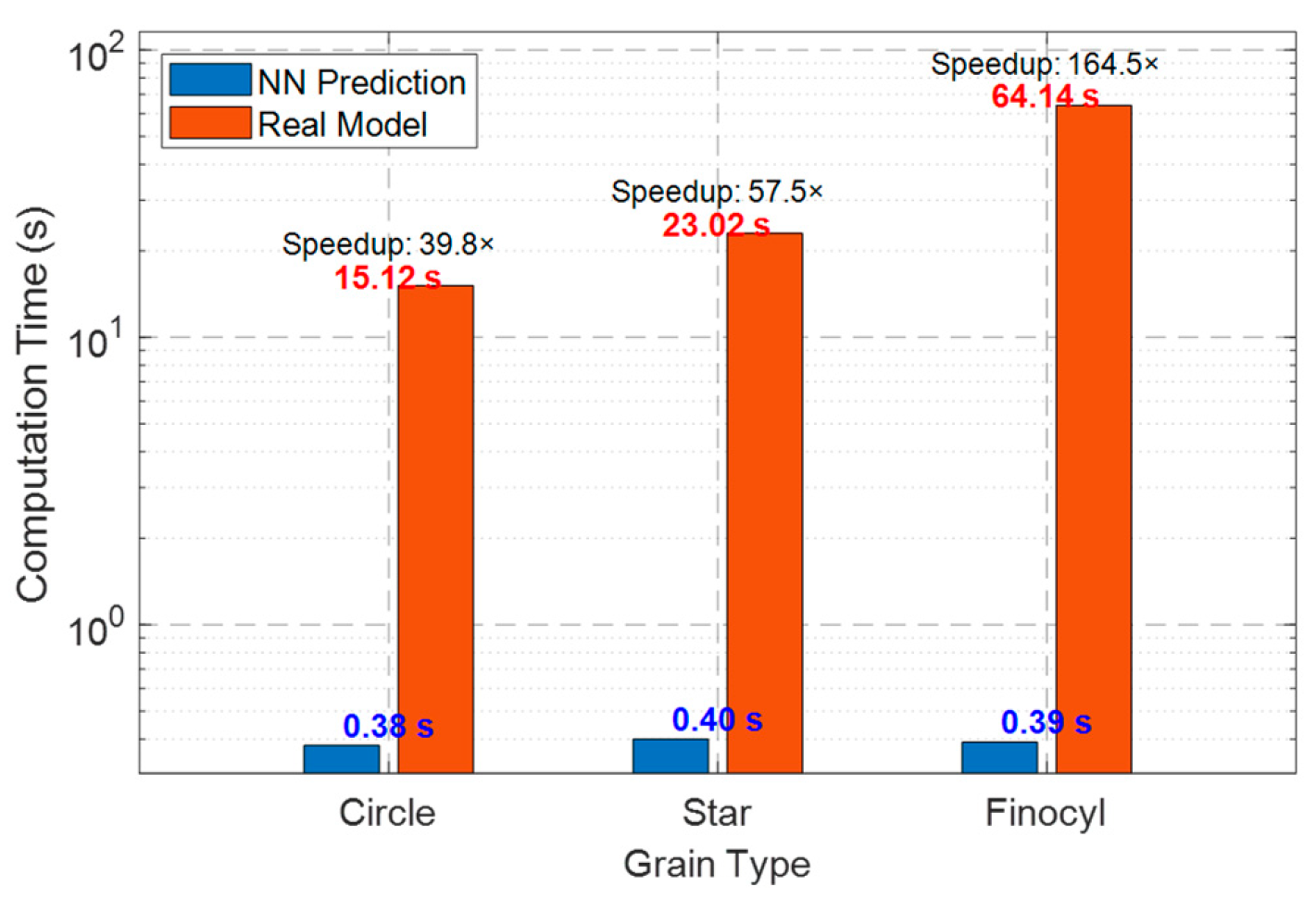
In addition, the calculation time of NN-enhanced performance prediction is compared with that of real models, as shown in Figure 11. It can be observed that the computation time of the NN prediction is significantly reduced, where the rapid prediction ability can be verified. As for the circle and star grains, the thrust calculation efficiency is improved by 39.8 and 57.5 times, respectively. Since the configuration of the finocyl grain is complex, the efficiency is improved most obviously, i.e., 164.5 times. The calculation time for all the grains is less than 0.5 s, demonstrating that the NN computation time is insensitive to the complexity of the grain geometry. It should also be noted that during thrust matching optimization, directly invoking the real model over 10,000 times leads to unaffordable computational costs. However, by replacing the real model with the NN, the optimization solution time can be drastically reduced.
Figure 11.
Time efficiency of NN-enhanced prediction.
5. Thrust Matching Optimization
Based on the developed trained neural network and thrust simulation model, the thrust matching optimization module is performed in this section, which aims to obtain the optimal solution that satisfies the specified requirements.
5.1. Thrust Matching Optimization Mathematical Model
The thrust matching optimization problem aims to simultaneously minimize the deviation between the mean thrust and the required one , and to reduce the gap between the mean thrust and the maximum one . Thus, the optimized thrust curve is close to the required thrust curve with smooth fluctuations. The constraints include the deviation between the working time and the required one , the ratio of real total impulse and theoretical one , the nozzle exit radius, the volumetric loading fraction , and the throat to port ratio . In addition to the grain configuration parameters, the throat radius and the expansion ratio are also considered as the design variables for optimization. Thus, the thrust matching optimization mathematical model is formulated in Equation (24).
In this paper, the design variables of the thrust matching optimization are listed in Table 4. It should be noted that the grain radius is a discrete variable due to limitations from the launch pipe. Similarly, the length is also constrained by the launch pipe, whose range is smaller than that presented in Table 1. Since the involved design variables consist of both continuous and discrete variables, the optimization in Equation (24) is a discrete–continuous mixed optimization problem.
Table 4.
Design variables of the thrust matching optimization problem.
5.2. Discrete–Continuous Mixed Differential Evolution Algorithm
To handle the different types of design variables in thrust matching optimization, this paper proposes a discrete–continuous mixed differential evolution algorithm (DCMDE). As a powerful and versatile heuristic optimization method, differential evolution (DE) has been widely applied to various practical engineering problems [22,23]. The differential evolution algorithm consists of four operators, i.e., initialization, mutation, crossover, and selection operators, cooperated with three control parameters including the scaling factor , crossover probability , and population size .
In DCMDE, the initialization operator is executed by the Latin hypercube sampling method [19], enhancing the spatial uniformity of the initial population. During the evolution process, the mutation, crossover, and selection operators are iteratively called to lead the population to the optimal region. For a given parent population, i.e., , the mutation operator used in this paper is the DE/Rand/1 strategy, which is combined with a round operator, expressed as
where , , and are distinct parent individuals randomly selected from ; denotes the dimensionality of the optimization problem; is the th mutant individual; is the th dimension value of .
The mutant individual is then intersected with the corresponding parent one to generate the trial individual , according to the following equation
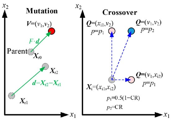
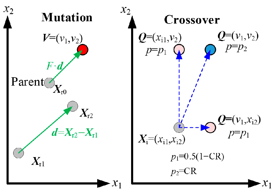
where is a random integer from 1 to , ensuring the distinction between and . The mutation and crossover operators are illustrated intuitively in Figure 12.
Figure 12.
Mutation and crossover operators.
Finally, the selection operator is applied to compare and based on the fitness values according to a predefined criterion, which is formulated as
In this paper, the feasibility rule is used to calculate the fitness value , which is described as follows [24]:
- (1)
- When comparing two feasible individuals, the individual with the superior objective value is selected.
- (2)
- When comparing two infeasible individuals, the individual with the smaller constraint violation value is selected.
- (3)
- A feasible individual is always preferred compared to an infeasible one.
6. Result Discussion
In this paper, NN-SRM is applied to two cases, which demonstrate the engineering practicality of NN-SRM. The information on the two cases and the parameter configuration is listed in Table 5.
Table 5.
Required thrust and optimization configuration.
6.1. Optimization and Analysis for Case 1
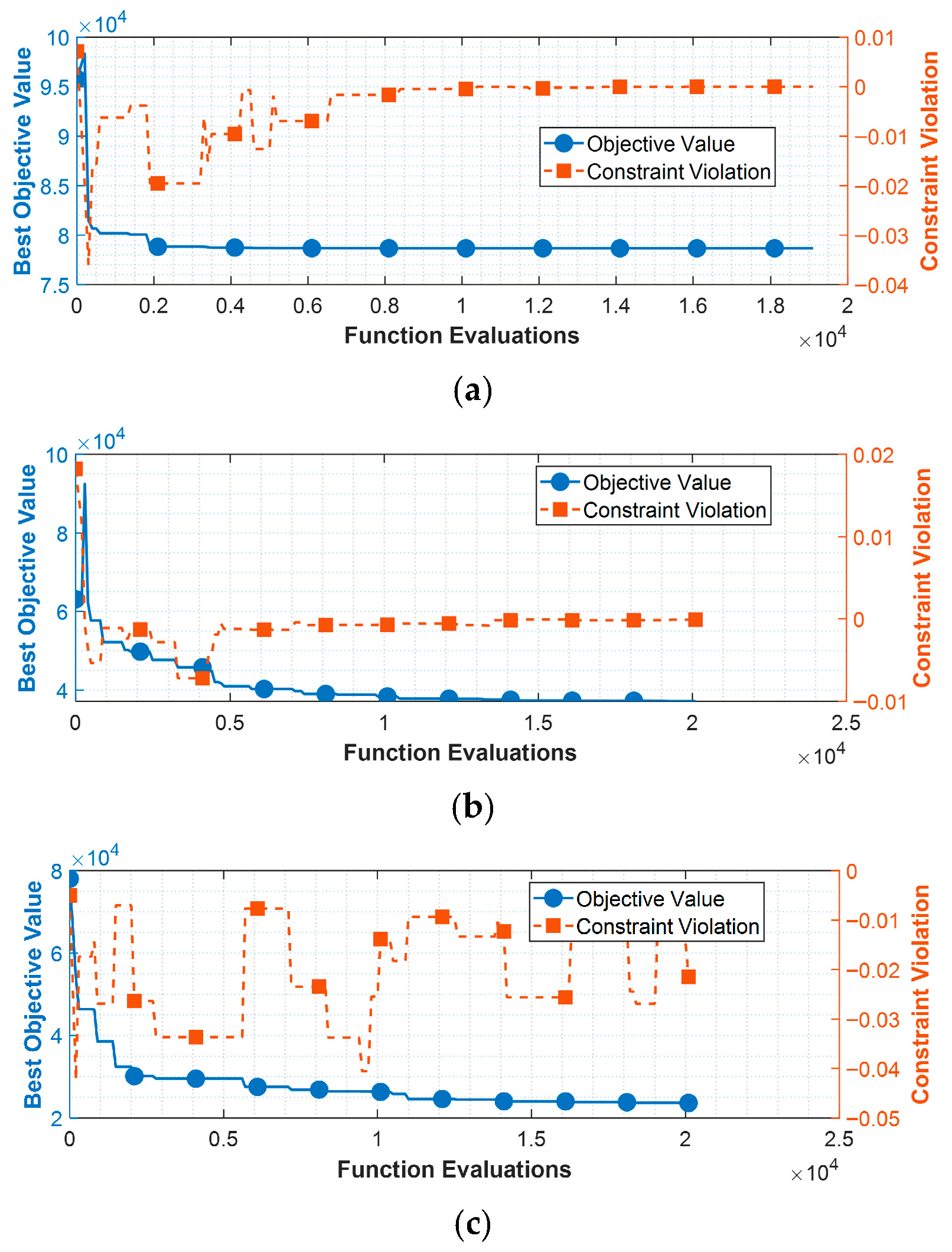
The convergence curves for Case 1 are presented in Figure 13, which indicates that DCMDE can converge to the feasible region for all grain categories. In the early stage of the optimization process, the solutions for the cylindrical and star grains are infeasible, causing DCMDE to prioritize reducing constraint violations initially, as illustrated in Figure 13a,b. When the number of function evaluations exceeds 10,000, i.e., in the medium stage, the three objective value curves gradually converge. The optimization results for three different grains are compared in Table 6. The thrust curves are presented in Figure 14.
Figure 13.
Optimization convergence curves for Case 1. (a) Cylindrical grain; (b) star grain; (c) finocyl grain.
Table 6.
Optimization result for Case 1.
Figure 14.
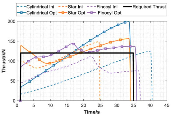
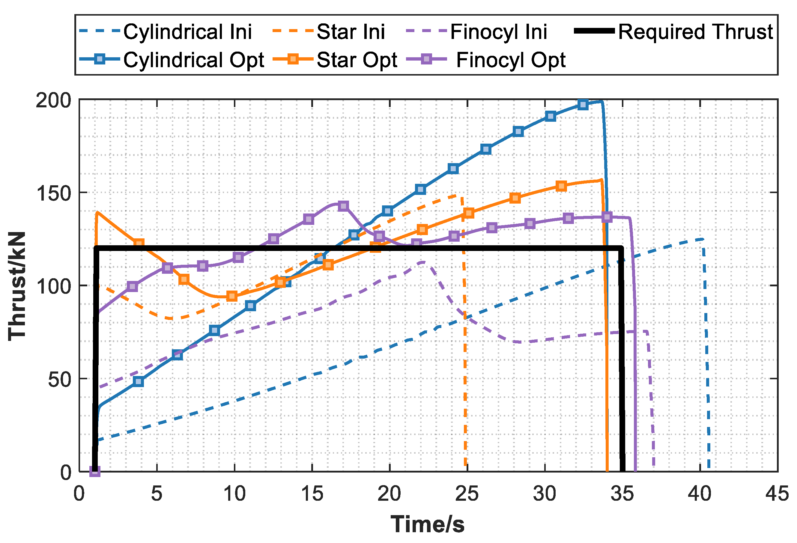
Thrust curves for Case 1.
From Table 6, it can be found that the finocyl grain achieves the best objective value among the three configurations. According to the optimized solution for the finocyl grain, the mean thrust is refined to 120.00 kN, matching the required thrust. However, the maximum thrust reaches 143.61 kN, which deviates slightly from the target value. The fin number and fin height ratio have been increased to ensure a large initial burning surface. Given the long required working time, the port radius has converged to the lower bound of 0.15, while the grain radius has reached the upper bound of 0.35 m, thereby increasing the burnback distance. As shown in Figure 14, the initial thrust curve of the finocyl grain is far from meeting the requirement. After optimization, the thrust can fluctuate slightly around the required value. Meanwhile, the working time is 35.82 s, within the required range of 35 ± 1 s.
Due to the similar configurations of the cylindrical and finocyl grains, their shared design variables, e.g., grain radius, port radius ratio, throat radius, and expansion ratio, have converged to close values. It should be noted that the cylindrical grain lacks mechanisms for adjusting the thrust curve, resulting in a thrust that increases in an approximately linear trend, as shown in Figure 14. For the star grain, the optimization process refines the configuration parameters to bring the thrust curve closer to the desired one, with the grain radius, star-edge angle, and star angle coefficient converging to their respective bounds. Due to the star’s disappearance, the thrust gradually increases after 10 s. The maximum thrust reaches 156.81 kN and leads to a larger objective value compared with that of the finocyl grain. In this case, the finocyl grain performs better than the star grain. The improvement ratio is 36.45%, which is calculated by
where 37.15 and 23.61 are the objective value of the best solutions by star and finocyl grains, as summarized in Table 6.
The real values of the objective and constraints are also calculated by invoking the grain geometry parametric model and provided in round brackets in Table 6. It can be observed that the relative errors for all terms are slight, i.e., less than 2%, demonstrating the effectiveness of NN-SRM.
6.2. Optimization and Analysis for Case 2
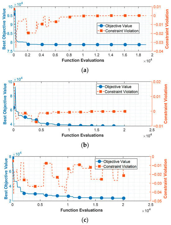
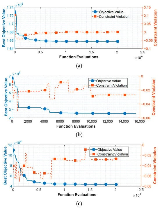
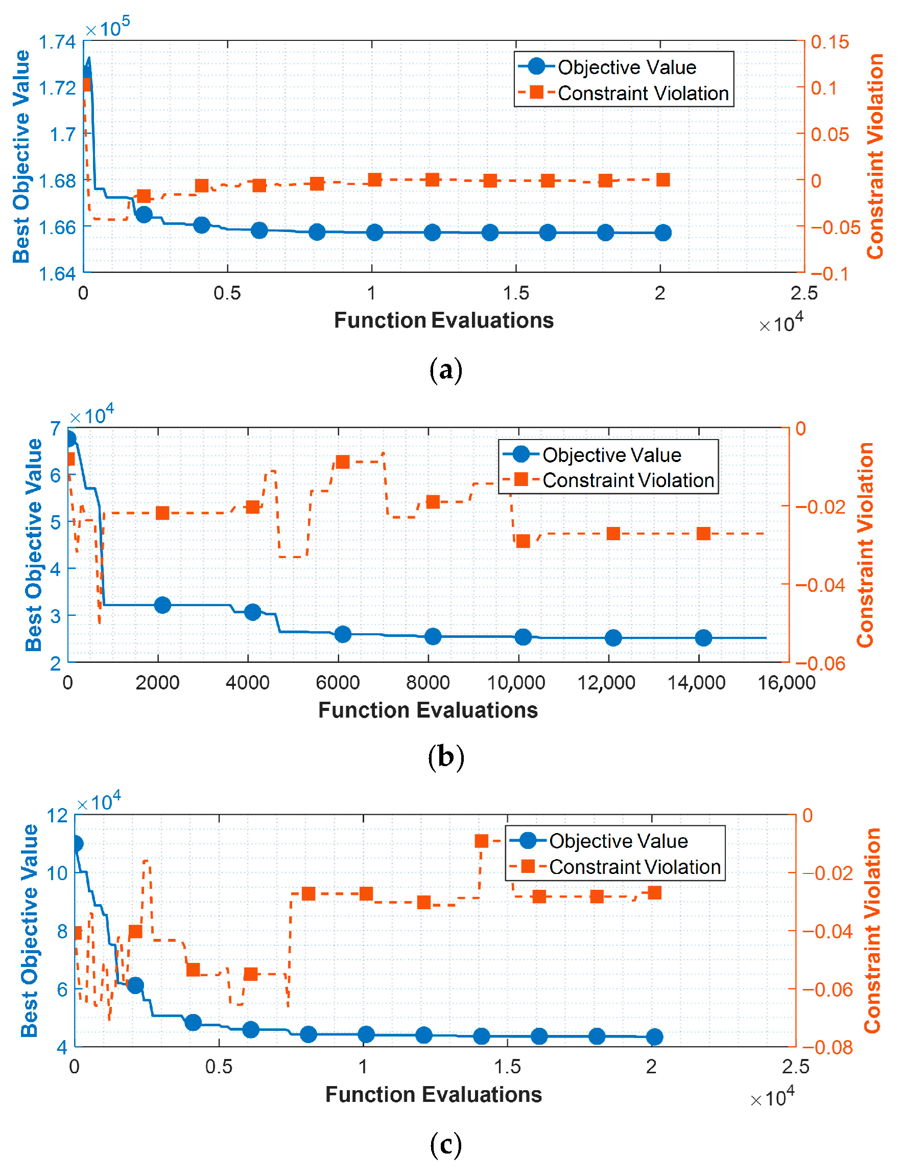
Unlike Case 1, Case 2 aims to optimize the grain to achieve a large thrust (180 kN) with a short working time (20 s). The optimization convergence curves for three grains are illustrated in Figure 15. Similar to Case 1, the cylindrical grain cannot adjust the thrust via its component, where the objective value is hard to optimize, as presented in Figure 15a. According to Figure 15b,c, both the star and finocyl grains can yield significant improvements for the objective within 10,000 function evaluations. The optimization results for three different grains are compared in Table 7. The thrust curves are presented in Figure 16.
Figure 15.
Optimization convergence curves for Case 2. (a) Cylindrical grain; (b) star grain; (c) finocyl grain.
Table 7.
Optimization result for Case 2.
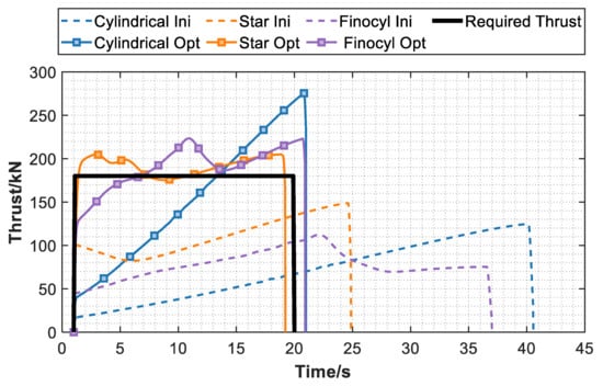
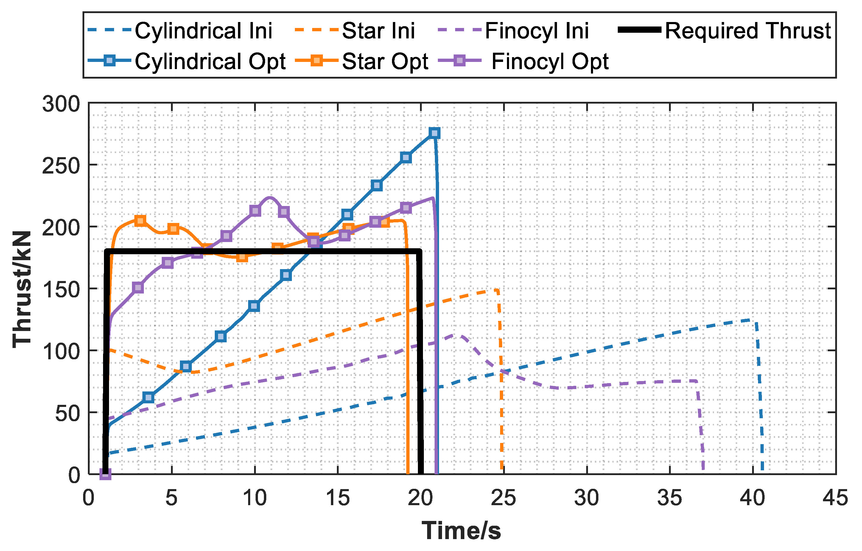
Figure 16.
Thrust curves for Case 2.
From Figure 15, the optimized star grain performs best among the competitors in Case 2, with a mean thrust of 180.12 kN and a maximum thrust of 206.05 kN, which are close to the requirements. According to Table 7, the characteristic length ratio reaches its upper bound to ensure a short working time under a grain radius of 0.35 m. This causes its loading fraction to be smaller than that of the other grains, while still satisfying the constraint.
In this case, the finocyl grain fails to yield a solution with a small thrust peak because of the limitation of the grain radius. When the optimized finocyl grain adopts a grain radius of 0.250 m, the mean value of the thrust fails to reach the desired level. The star grain performs better than the finocyl one. The improvement ratio is 41.86%, which is calculated by
where 43.35 and 25.19 are the objective value of the best solutions by finocyl and star grains, as summarized in Table 7.
Comparing the values obtained from NNs and real geometric models, the relative errors in the mean and maximum thrusts remain at a low level, i.e., below 2%. These two cases have demonstrated the approximation accuracy of the trained NN in predicting the burning surface, free volume, and grain volume. Simultaneously, it can be concluded that various grain configurations are necessary to identify the best thrust solution, satisfying different requirements.
7. Conclusions
To rapidly predict thrust performance and obtain a solution that satisfies the requirements, this paper develops a neural network-enhanced rapid performance prediction and matching optimization framework for solid rocket motors (NN-SRM). The neural networks are utilized to approximate the burnback process of cylindrical, star, and finocyl grains. The trained neural network achieves promising approximation accuracy, with an R2 value exceeding 0.95 for all crucial parameters. Thrust is then obtained by combining zero-dimensional internal ballistics equations and one-dimensional steady isentropic flow relations. A discrete–continuous mixed differential evolution algorithm is also developed to capture the best grain configuration and nozzle parameters. The optimization results illustrate that the finocyl grain performs 36.45% better than the star grain for small thrust (120 kN) and long working time (35 s). For large thrust (180 kN) and short working time (20 s), the star grain can yield a solution that is 41.86% better than the finocyl grain.
In this work, the nozzle throat ablation, variable specific rate and complex vertical flows are ignored, which are required to be improved in future. Secondly, the authors will focus on integrating additional grain configuration categories into the NN-SRM. Furthermore, the dual-burning-rate internal ballistic equations and six-degree-of-freedom trajectory equations need to be further investigated, which is essential for the preliminary design of flight vehicles.
Author Contributions
Conceptualization, N.Y. and R.S.; methodology, N.Y.; validation, R.S. and S.L.; formal analysis and investigation, D.G. All authors have read and agreed to the published version of the manuscript.
Funding
This study was supported by the National Natural Science Foundation of China (grant numbers 92371101) and the Foundation of Key Laboratory of National Key Laboratory of Land and Air Based Information Perception and Control (Grant No. B12503).
Data Availability Statement
The NN-SRM proposed in this paper can be replicated by implementing the steps as shown in Section 3, Section 4 and Section 5. For the convenience of readers, the trained neural network data for three grains are available in the supplement. However, the source code cannot be made publicly available due to confidentiality restrictions. If there is any confusion about the method, we welcome inquiries and are pleased to help.
Conflicts of Interest
The authors declare no conflicts of interest.
Abbreviations
The following abbreviations are used in this manuscript:
| SRM | Solid rocket motor |
| NN | Neural network |
| LSTM | Long short-term memory |
| DCMDE | Discrete–continuous mixed differential evolution |
| NN-SRM | Neural network-enhanced framework for solid rocket motors |
References
- Baiserikov, B.; Ismailov, M.; Mustafa, L.; Yesbolov, N.; Kulbekov, A.; Yermekov, A.; Meiirbekov, M.; Ablakatov, I. Design and Manufacturing of Experimental Solid Propellant Rocket Motor Cases Made of Carbon Composite Materials. Polymers 2025, 17, 1352. [Google Scholar] [CrossRef] [Scilit] [PubMed]
- Fan, X.; Wei, R.; He, Y.; Hui, W.; Zhao, W.; Bao, F.; Hou, X.; Sun, L. Multi-Objective Design Optimization of Solid Rocket Motors via Surrogate Modeling. Aerospace 2025, 12, 805. [Google Scholar] [CrossRef] [Scilit]
- Kamran, A.; Guozhu, L. An integrated approach for optimization of solid rocket motor. Aerosp. Sci. Technol. 2012, 17, 50–64. [Google Scholar] [CrossRef] [Scilit]
- Mahjub, A.; Mazlan, N.M.; Abdullah, M.Z.; Azam, Q. Design Optimization of Solid Rocket Propulsion: A Survey of Recent Advancements. J. Spacecr. Rocket. 2019, 57, 3–11. [Google Scholar] [CrossRef] [Scilit]
- Williams, A.; Himschoot, A.; Saafir, M.; Gatlin, M.; Pendleton, D.; Alvord, D.A. A Machine Learning Approach for Solid Rocket Motor Data Analysis and Virtual Sensor Development. In AIAA Propulsion and Energy 2020 Forum; AIAA Propulsion and Energy Forum; American Institute of Aeronautics and Astronautics: Reston, VA, USA, 2020. [Google Scholar]
- Zhang, W.; Xu, M.; Yang, H.; Wang, X.; Zheng, S.; Li, X. Data-driven deep learning approach for thrust prediction of solid rocket motors. Measurement 2024, 225, 114051. [Google Scholar] [CrossRef] [Scilit]
- Lee, H.S.; Kwon, S.W.; Lee, J.S. Neural networks for the burn back performance of solid propellant grains. Aerosp. Sci. Technol. 2023, 137, 108283. [Google Scholar] [CrossRef] [Scilit]
- Korompili, G.; Cholevas, N.; Anyfantis, K.N.; Mußbach, G.; Riziotis, C. Structural Diagnosis of Solid Rocket Motors Using Neural Networks and Embedded Optical Strain Sensors. Photonics 2024, 11, 799. [Google Scholar] [CrossRef] [Scilit]
- Liu, D.; Sun, L.; Miller, T.C. Defect Diagnosis in Solid Rocket Motors Using Sensors and Deep Learning Networks. AIAA J. 2020, 59, 276–281. [Google Scholar] [CrossRef] [Scilit]
- Yu, X.; Hu, Y.; Guo, R.; Fan, L.; Ding, H.; Xiao, J. Review of physics-informed neural networks in hemodynamics. Eng. Appl. Artif. Intell. 2026, 163, 112834. [Google Scholar] [CrossRef] [Scilit]
- Dai, E.; Xu, H.; Wei, H.; Cai, G. Real-time Trajectory Generation for Hypersonic Vehicles Based on Improved PSO-BP Neural Network⁎⁎This work was supported by the National Natural Science Foundation of China under Grant 62473374, Grant 62403487, and Grant U2441243. IFAC-PapersOnLine 2025, 59, 928–933. [Google Scholar] [CrossRef] [Scilit]
- Geisler, R.L.; Frederick, R.A., Jr.; Giarra, M. Historical Overview and Solid Rocket Motor Fundamentals. In Encyclopedia of Aerospace Engineering; Wiley: Hoboken, NJ, USA, 2010. [Google Scholar]
- Zeping, W.; Donghui, W.; Weihua, Z.; Okolo, N.P.; Yang, F. Solid-Rocket-Motor Performance-Matching Design Framework. J. Spacecr. Rocket. 2017, 54, 698–707. [Google Scholar] [CrossRef] [Scilit]
- Li, W.; He, Y.; Zhang, Y.; Liang, G. Design and Optimization of Modular Solid Rocket Grain Matching Multi-Thrust Performance Curve. Appl. Sci. 2025, 15, 6827. [Google Scholar] [CrossRef] [Scilit]
- Kim, E.; Joo, S.; Oh, S. Inverse design framework for optimizing solid propellant grains toward target performance profiles. Acta Astronaut. 2026, 238, 645–656. [Google Scholar] [CrossRef] [Scilit]
- Ren, J.; Wei, R.; Bao, F.; Hou, X. An Interval Analysis Method for Uncertain Multi-Objective Optimization of Solid Propellant Formulations. Aerospace 2025, 12, 865. [Google Scholar] [CrossRef] [Scilit]
- Wu, Y.; Quan, S.J. A review of surrogate-assisted design optimization for improving urban wind environment. Build. Environ. 2024, 253, 111157. [Google Scholar] [CrossRef] [Scilit]
- Viana, F.A.C.; Gogu, C.; Goel, T. Surrogate modeling: Tricks that endured the test of time and some recent developments. Struct. Multidiscip. Optim. 2021, 64, 2881–2908. [Google Scholar] [CrossRef] [Scilit]
- Wang, Q.; Nakashima, T.; Lai, C.; Mutsuda, H.; Kanehira, T.; Konishi, Y.; Okuizumi, H. Modified Algorithms for Fast Construction of Optimal Latin-Hypercube Design. IEEE Access 2020, 8, 191644–191658. [Google Scholar] [CrossRef] [Scilit]
- Wu, D.; Huang, H.; Qiu, S.; Liu, Y.; Wu, Y.; Ren, Y.; Mou, J. Application of Bayesian regularization back propagation neural network in sensorless measurement of pump operational state. Energy Rep. 2022, 8, 3041–3050. [Google Scholar] [CrossRef] [Scilit]
- Abbas, M.; Medani, M.; Rajab, A.B.; Elaissi, S.; Zayani, H.M.; Faiz, Z.; Khan, I.; Ben Khedher, N. Computational intelligence of Bayesian regularization backpropagation neural networks to study the thermo-bioconvection flow of hybrid-nanofluid with thermal Radiation: Biotechnological perspectives. J. Radiat. Res. Appl. Sci. 2025, 18, 101777. [Google Scholar] [CrossRef] [Scilit]
- Storn, R.; Price, K. Differential evolution–a simple and efficient heuristic for global optimization over continuous spaces. J. Glob. Optim. 1997, 11, 341–359. [Google Scholar] [CrossRef] [Scilit]
- Ahmad, M.F.; Isa, N.A.M.; Lim, W.H.; Ang, K.M. Differential evolution: A recent review based on state-of-the-art works. Alex. Eng. J. 2022, 61, 3831–3872. [Google Scholar] [CrossRef] [Scilit]
- Rahimi, I.; Gandomi, A.H.; Chen, F.; Mezura-Montes, E. A Review on Constraint Handling Techniques for Population-based Algorithms: From single-objective to multi-objective optimization. Arch. Comput. Methods Eng. 2023, 30, 2181–2209. [Google Scholar] [CrossRef] [Scilit]

Disclaimer/Publisher’s Note: The statements, opinions and data contained in all publications are solely those of the individual author(s) and contributor(s) and not of MDPI and/or the editor(s). MDPI and/or the editor(s) disclaim responsibility for any injury to people or property resulting from any ideas, methods, instructions or products referred to in the content. |
© 2026 by the authors. Licensee MDPI, Basel, Switzerland. This article is an open access article distributed under the terms and conditions of the Creative Commons Attribution (CC BY) license.