Design and Simulation Analysis of Attitude Control Algorithms for OPS-SAT-1

Abstract

This work presents the design of an attitude control experiment for onboard OPS-SAT-1 satellite execution, conceived with inherent extensibility to future mission architectures. OPS-SATs are ESA nanosatellite mission series designed as an in-orbit testbed for validating novel software and control techniques under real space conditions, OPS-SAT-1 being the first mission. Equipped with an advanced payload computer, OPS-SAT-1 enabled experimentation with innovative mission operations, including real-time attitude control strategies. Two attitude control algorithms, a modified Proportional–Integral–Derivative (mPID) and a fuzzy logic controller, were designed and implemented for the OPS-SAT-1. The design methodology applied to these controllers consisted of (i) modelling the space environment and satellite characteristics, (ii) assessing actuator feasibility, (iii) determining the operational ranges for attitude error and angular velocity, (iv) parametrizing controllers within these ranges, (v) fine-tuning controllers using multi-objective genetic optimization, and (vi) robustness analysis using the Monte Carlo method. Despite the technical issues related to communication with the OPS-SAT-1 hardware, which prevented the execution of the experiment in orbit, this work presents the simulation results that were obtained. These results indicate that fuzzy logic controllers may outperform PID controllers in terms of the accumulated error, settling time and steady-state error, whereas power efficiency appears to be less robust than in the PID. This suggest that a large uncertainty in the model could lead the PID to become more efficient. Near the nominal scenario, the fuzzy controller achieves superior error–cost trade-offs, enabling precise attitude stabilization with lower energy consumption. These findings suggest the potential advantages of modern control approaches compared to classical methods, which will be further assessed through future in-orbit experiments.

1. Introduction

The evolution of the space sector over the last two decades has been marked by a paradigm shift towards platform miniaturization, giving rise to nanosatellites and, specifically, the CubeSat standard. These small satellites, typically weighing between 1 and 10 kg, have transitioned from educational tools to sophisticated platforms for Earth observation, telecommunications, and scientific research [1]. However, this trend towards miniaturization introduces significant engineering challenges, particularly in the design and implementation of the Attitude Determination and Control Subsystem (ADCS). This is especially critical for mission success because maintaining a precise orientation in space directly affects solar panel alignment, antenna pointing accuracy, and payload stability.

In the Low Earth Orbit (LEO) environment—where most nanosatellites operate—the spacecraft is exposed to various environmental disturbances, including aerodynamic drag, solar radiation pressure, magnetic residual dipoles, and gravity gradient torques. These nonlinear effects complicate the design of robust and efficient control algorithms. Consequently, improving the performance of the ADCS is not just a technical enhancement but a mission-critical necessity.

Traditionally, classical controllers such as Proportional–Integral–Derivative (PID) algorithms [2,3,4] have dominated space applications due to their simplicity and proven reliability. Although effective near equilibrium points, these controllers often struggle with the nonlinear and time-varying nature of real-world orbital dynamics [1]. In recent years, more advanced strategies have expanded, such as $H_{\infty }$ control [5], Sliding Mode Control [6,7], Model Predictive Control (MPC) [8,9,10,11] and Artificial Intelligence (AI)-based techniques, including fuzzy logic [12,13,14,15,16,17,18] and neural networks [19,20,21]. Among these, fuzzy logic stands out for its ability to handle nonlinear systems while requiring relatively low computational resources.

Fuzzy Logic Control (FLC), grounded in Zadeh’s theory of fuzzy sets [22], allows for flexible rule-based control that mimics human reasoning and accommodates uncertainties. Despite its theoretical advantages and demonstrated success when used for satellite attitude control [1,23,24,25,26], the adoption of FLC in aerospace has been limited, mainly due to the conservative nature of the space industry and the high reliability standards required for flight systems. For FLC to be considered viable, extensive simulation and, crucially, in-orbit validation are essential.

This study addresses this gap by presenting the design, simulation-based evaluation and implementation of a fuzzy logic-based ADCS for the OPS-SAT-1 mission of the European Space Agency (ESA). OPS-SAT-1 was a 3U CubeSat designed as an open and reprogrammable platform for testing experimental software in orbit. Its architecture ensures satellites’ safety during experimental runs, making it an ideal testbed for innovative control strategies.

Our proposed experiment involved implementing two control strategies onboard OPS-SAT-1: a fuzzy logic controller and a modified PID (mPID) controller. Both controllers were tuned using multi-objective genetic optimization based on a satellite dynamics model adapted for OPS-SAT-1. The performance metrics evaluated included point accuracy, response time, and energy efficiency—key considerations for missions with limited power budgets. The experiment was configured to execute a predefined sequence of attitude maneuvers using each controller. Together with the controller design, a novel in-orbit application was built on the ESA Nanosat Mission Operations Framework in Java. Although the experiment could not be successfully executed due to an I2C communication issue onboard, the developed application can be readily implemented on any satellite adopting a similar pointing strategy and based on the same Service-Oriented Architecture, which constitutes the baseline architecture for upcoming ESA nanosatellite missions [27]. The same applies to controller design; the methodology adopted in this work is readily transferable to other spacecraft platforms. Consequently, the experimental design is directly reusable for future platforms, in particular, for future OPS-SAT, VOLT, ORIOL or PRETTY missions.

The article is organized as follows. Section 2 presents the OPS-SAT-1 platform and the simulation environment. Section 3 describes the design and tuning of the controllers. Section 4 presents the main results derived from the numerical simulations. Section 5 describes the experimental protocol. Finally, Section 6 presents the discussion and conclusions.

2. Materials and Methods

2.1. Experimental Platform

OPS-SAT-1 was a 3U CubeSat developed by the ESA to serve as a highly flexible in-orbit laboratory for the validation of experimental mission software [28]. Unlike typical CubeSat, which is often limited by its onboard processing capabilities, OPS-SAT-1 was equipped with a cutting-edge flight computer that offered significantly enhanced performance and reconfigurability. This capability enabled the real-time execution of complex algorithms and the remote modification of onboard applications, making it ideal for testing advanced control strategies, including those not yet qualified for flight in operational missions.

The mission architecture included safety mechanisms to ensure that the satellite could recover from anomalous behavior caused by experimental software. This fault tolerance was critical for allowing unproven control algorithms to be evaluated in a real space environment without risking mission failure. The OPS-SAT-1 subsystem design, which included a high-precision ADCS, supported experiments that required fine control authority and telemetry resolution.

The characteristics that define this scenario are summarized in Table 1.

Table 1. Parameters of OPS-SAT-1 simulation scenario.

Parameter	Subparameter	Value	Unit
Satellite Characteristics
Geometry	Y-Positive Panel	0.01 × 0.2 × 0.3	[m]
	Central body	0.1 × 0.1 × 0.3
	Y-Negative Panel	0.01 × 0.2 × 0.3
Inertia matrix	$\left[\begin{array}{ccc}+6.58\times {10}^{+1}& +2.58\times {10}^{-3}& +2.34\times {10}^{-1}\\ +2.58\times {10}^{-3}& +5.65\times {10}^{+1}& +5.45\times {10}^{-2}\\ +2.34\times {10}^{-1}& +5.45\times {10}^{-2}& +1.65\times {10}^{+1}\end{array}\right]\times {10}^{-3}$		[kg·m2]
6 × Reaction wheels	Max speed	10,000	[rpm]
	Max torque	$1.0\times {10}^{-4}$	[N·m]
	Max momentum	$1.5465\times {10}^{-6}$	[kg·m2]
3 × Magnetorquers	X, Y axes	0.2	[A·m2]
	Z axis	0.1
Drag coefficient		2.0	N/A
Reflectivity coefficient		1.0	N/A
Residual dipole		$\left[111\right]\times {10}^{-7}$	[A·m2]
Orbital Characteristics (from TLE data)
Eccentricity		0.0013748	N/A
Inclination		97.4697	[deg]
Right ascension		141.5292	[deg]
Argument of perigee		186.0985	[deg]
Mean motion		15.1579775	[rev/day]
Mean anomaly		174.0082	[deg]
Initial epoch		22 March 2021 22:45:00	UTC

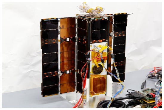
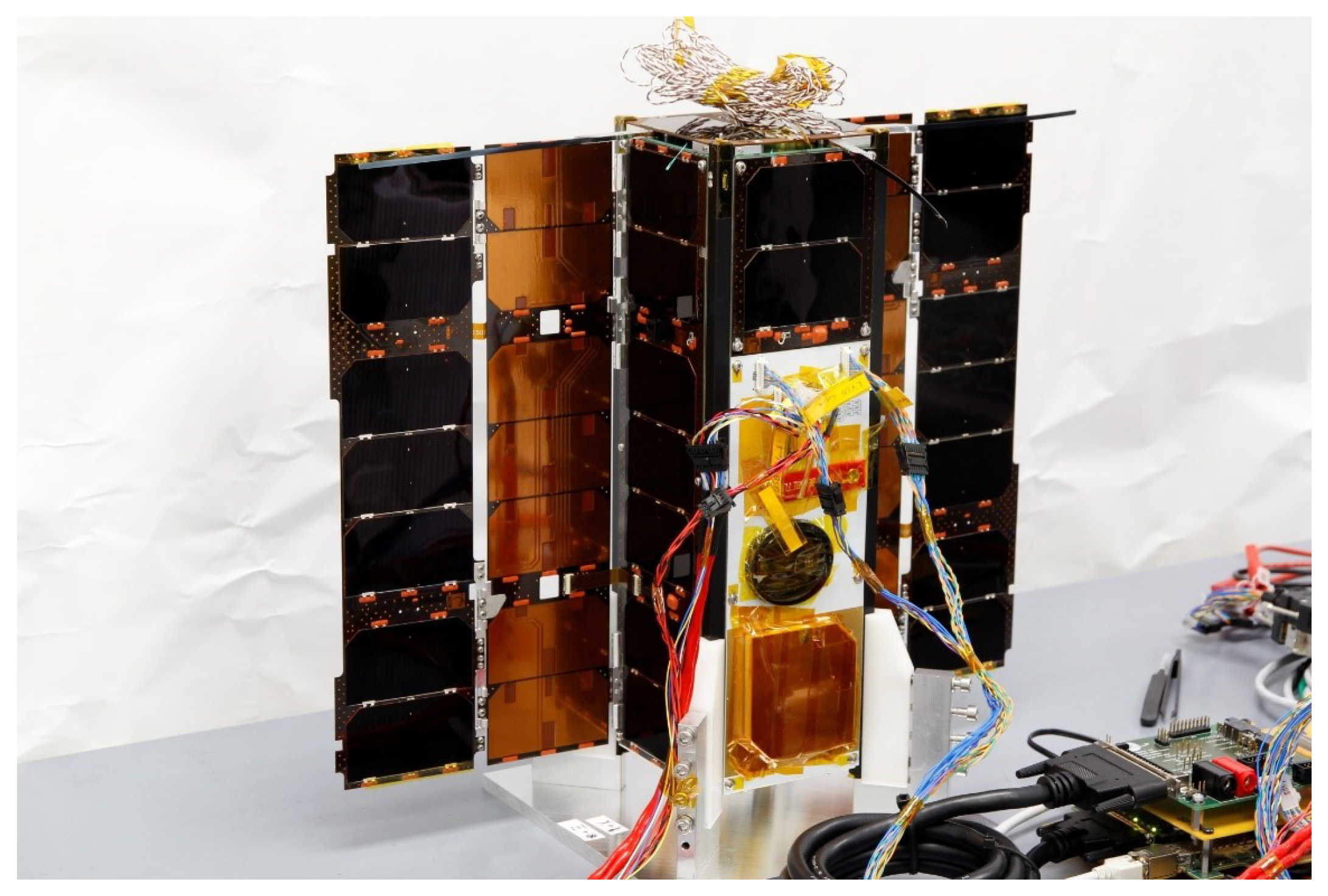
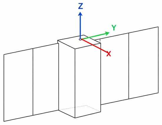
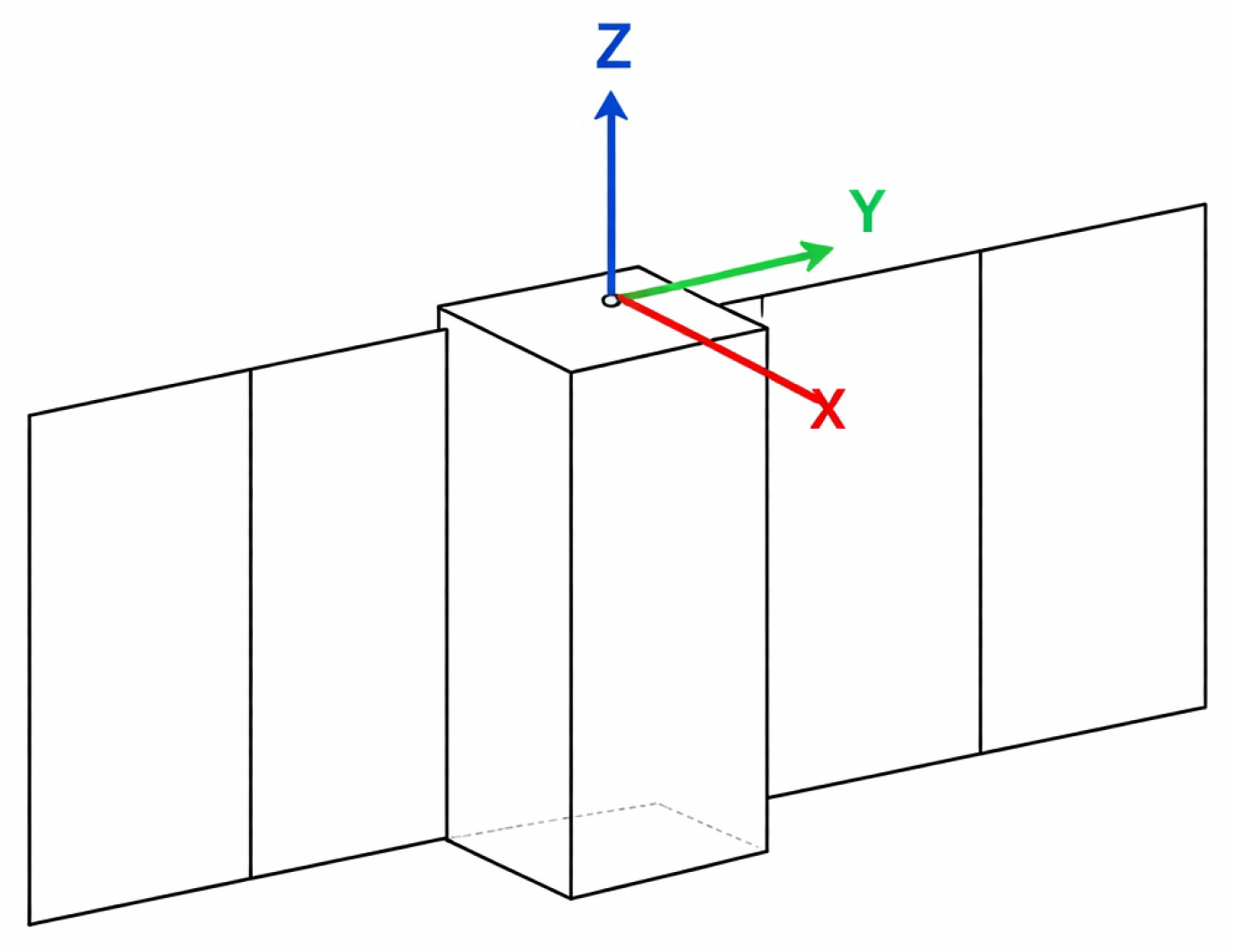
The geometry and inertial properties of the satellite are modeled in detail as part of the simulation framework for the experiment (see Section 2.2). According to the platform data, the OPS-SAT-1 structure comprises a central body with dimensions of 0.1 × 0.1 × 0.3 m³ and two lateral panels of 0.01 × 0.2 × 0.3 m³ (see Figure 1). All the faces of the satellite are equipped with solar cells; however, the main solar array is located on the − X face of OPS-SAT-1 (see colored axes in Figure 2). On the opposite face (+X), the star tracker sensor is plcaed. The +/−Y axis corresponds to the direction in which the satellite’s lateral panels have been deployed, forming a relatively large surface parallel to the YZ plane. The +/−Z direction defines the longitudinal axis of the satellite, with the +Z face hosting the deployable UHF antenna. Tthe L-band antenna—primarily used to monitor OPS-SAT-1 is located on the −Z face. In the nominal attitude mode, the satellite is required to keep its Z axis of the body aligned with the local vertical, with the negative direction (−Z) pointing towards the nadir. This orientation maximizes the performance of the primary communication antenna, ensuring its optimal connectivity with ground stations. In addition to this constraint, the satellite must minimize the solar incidence angle with respect to the YZ plane, i.e., it should maximize the solar flux incident on the face containing the main solar array (−X face), which is nominally aligned with the Sun’s direction.

Figure 1. OPS-SAT-1 during testing of its solar arrays at the Graz University of Technology, Austria. Courtesy of ESA, OPS-SAT team and TU Graz.

Figure 2. Diagram of OPS-SAT-1 showing the front view and the triad parallel to the body frame.

It is important to highlight the significant variation in the exposed surface area of the satellite depending on its orientation. This “wetted surface area” is a key parameter when considering the effects of aerodynamic and solar radiation pressure perturbations. In the nominal attitude, the −Y direction forms a relatively small angle with the orbital velocity vector, resulting in an aerodynamic wetted surface area of approximately 3.0 × 10⁻² m². Rotations around the Z axis increase this value, potentially reaching 1.5 × 10⁻¹ m². In contrast, rotations around the X axis can reduce it to 1.0 × 10⁻² m². A similar trend is observed with solar perturbations: in the nominal attitude, the −X direction forms a small angle with the solar vector, producing a solar-wetted area of approximately 1.5 × 10⁻¹ m². Rotations around the Z and Y axes can decrease this solar-exposed area to 3.0 × 10⁻² m² and 1.0 × 10⁻² m², respectively. Awareness of the potential magnitude of these perturbations is essential to ensure that the satellite’s actuators are capable of counteracting the resulting disturbance torques under the most adverse conditions.

The ADCS of OPS-SAT-1 includes six reaction wheels arranged in a redundant configuration, with a maximum speed of 10,000 rpm and a torque capability of 1.0 × 10⁻⁴ N · m. This configuration allows for precise three-axis control and enables the application of complex attitude maneuvers without the risk of actuator saturation under nominal conditions. Furthermore, OPS-SAT-1 includes three orthogonal magnetorquers used for momentum unloading and coarse attitude correction. The inclusion of both types of actuator enhances the controllability of the satellite and allows for comparative studies of the control efficiency under various disturbance rejection scenarios. These actuators will be leveraged during the experiment to test both the mPID and fuzzy logic controllers in a range of pre-programmed maneuvers (see Section 5 for more detail).

The satellite was injected into a 6–18 Sun-synchronous orbit (also known as a “dusk–dawn” orbit), in which the sub-satellite point follows the Earth’s regions transitioning between day and night. In this orbital configuration, the Sun direction remains approximately 90° from the local vertical and lies in a direction normal to the orbital plane. Ideally, this results in a zero solar incidence angle relative to the −X face, which hosts the primary solar array. However OPS-SAT-1 lacks onboard propulsion and therefore cannot perform orbital corrections. As a result, minor injection errors during launch or the long-term accumulation of orbital perturbations may lead to a non-zero solar incidence angle on the main solar array. In practice, OPS-SAT-1 can reduce its angular velocity and reorient itself using stored battery energy without needing to adjust the orientation of its solar panels. Nevertheless, the described reference system is used to define and constrain the satellite’s nominal orientation states.

2.2. Simulation Environment

To be able to tune and test different algorithms in the control block, it is necessary to have a plant on which to act. In the aerospace industry in general, and particularly when designing satellite attitude control algorithms, it is not feasible to use the real plant for testing purposes. In addition, during the early stages of design, many of the satellite’s design parameters are only loosely defined, which means that they may be updated or changed radically at some point. These changes can have a critical impact on the attitude control system.

For all these reasons, it is essential to have a simulator that models the satellite specifications, its rotational dynamics, and its environmental conditions, but above all that is capable of modifying and adjusting its simulation conditions in response to design changes. This type of simulator can range from simple rigid-body equations in a vacuum to complex simulators that include numerous disturbance elements, as well as more comprehensive satellite models.

For the design and verification of the attitude controllers studied in this work, a numerical simulation platform has been used, developed from the DKE simulator (Dynamics, Kinematics and Environment) used in [1], but including the characteristics of the OPS-SAT-1 operational scenario. The moment of inertia tensor, the actuator’s performance characteristics (reaction wheels and magnetorquers), and other physical parameters of the OPS-SAT-1 were integrated into the simulation environment to replicate the flight conditions as accurately as possible. This numerical environment acts as the plant that, through simulations under different operational and environmental conditions, transforms the output signals of the attitude controller into a new state of the system.

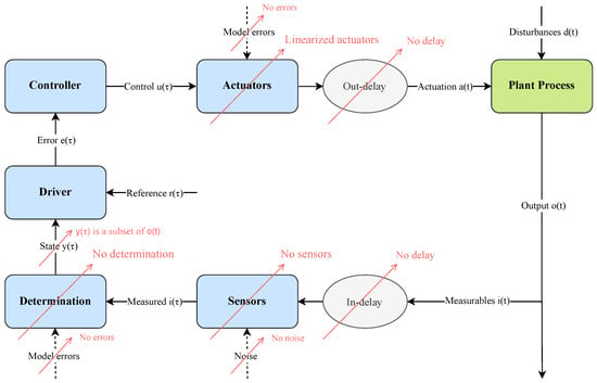
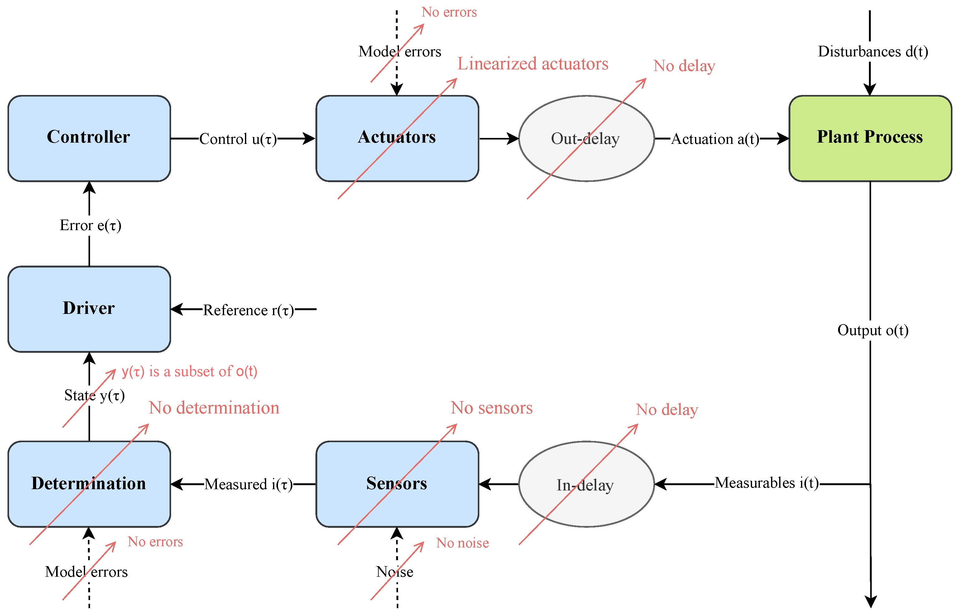
The simulation environment models the following elements of the control loop shown in Figure 3: the sensor and attitude determination blocks; the actuator block; and the environment, which includes the attitude dynamics of the vehicle as a function of its mass properties and external torques. The model has been simplified to focus only on the effect that having different control signals has on the performance of the attitude system. Figure 3 outlines how the simulator’s capabilities have been simplified. It has been assumed, within the simulations, that the satellite has knowledge of the true state of the system, that is, that the sensor and determination blocks are treated transparently, without modeling the errors or delays in the attitude signal. With respect to actuators, it has been assumed that their behavior is linear with respect to the control input signal but taking into account the saturation limits. That is, the control signal is considered to perfectly modulate this actuation variable within the predefined operational limits of each actuator.

Figure 3. Schema of the simulation environment.

Simulations have been performed using @MATLAB R2022a. The simulation environment for both controllers is the same; the only difference is the content of the “controller” box. The controllers compute the control signal, u, by monitoring an input signal: the error signal, e. This signal is constructed in the “driver” block as the difference between the process variable to be controlled, y (the output of the determination block), and a reference signal or a “set point”, r. In a real control process, all signals that are functions of time t (actuations a, disturbances d, outputs o, and estimated variables i) are truly continuous-time functions. However, in the simulator, these functions are not continuous, but are rather samples of values at intervals given by the simulation time step, $\mathrm{\Delta }t$. Similarly, both in a real control process and within the simulator, signals that are functions of time $\tau$ (the state y, the reference r, the error e, and the control u) are discrete values spaced by the control time step $\mathrm{\Delta }\tau$. Throughout all the simulations presented in this work, the control time step has been imposed to be at least one order of magnitude larger than the simulation time step; that is, $\mathrm{\Delta }t$ = o($\mathrm{\Delta }\tau$).

The environment model implements a numerical integrator of the typical dynamic Euler equations of a rigid body that contains momentum exchange devices (inertia wheels):

$$\dot{\mathit{\omega }}={\left(I_S^B\right)}^{-1}·(\mathit{T}-\mathit{\omega }\times (I_S^B·\mathit{\omega })+{\mathit{T}}_{C,int}+{\mathit{T}}_{D,int}),$$

(1)

$${\mathit{T}}_{C,int}=-\sum _{i=1}^N(I_i^B·\dot{{\mathit{\omega }}_i}),$$

(2)

$${\mathit{T}}_{D,int}=-\mathit{\omega }\times \sum _{i=1}^N(I_i^B·\dot{{\mathit{\omega }}_i});$$

(3)

where $\mathit{\omega }$ is the satellite angular velocity, $I_S^B$ is the inertia tensor of the satellite calculated with respect to its center of mass, $\mathit{T}$ is the external torque, ${\mathit{T}}_{C,int}$ is the internal control torque, ${\mathit{T}}_{D,int}$ is the internal disturbance torque, $I_i^B$ is the inertia tensor of each momentum exchange device calculated with respect to the center of mass of the satellite, ${\mathit{\omega }}_i$ is the angular velocity of each momentum exchange device, and N is the total number of momentum exchange devices that the satellite has. All vectorial quantities are expressed in body coordinates. For the external torque’s contribution to dynamics, the usual four main disturbance contributions have been taken into account: aerodynamic drag, solar radiation pressure, gravity gradient, and residual dipole. These equations are closed with

$${\displaystyle \frac{d{q}_{IB}}{dt}}={\displaystyle \frac{1}{2}}{q}_{IB}\ast \left[\begin{array}{cc}0& \mathit{\omega }\end{array}\right]$$

with $q_{IB}$ being the attitude quaternion of the inertial frame with respect to the body frame.

3. Controller’s Design

3.1. Default Controller

The purpose of this controller is to standardize the initial conditions of the experiment to be conducted on OPS-SAT-1, specifically by ensuring that the maneuvers can begin with a sufficient actuation capacity to be completed without saturating the angular velocity of the reaction wheels. Additionally, it aims to align the body reference frame with the nominal attitude reference—determined by the Sun and nadir directions—so that the maneuvers start as close as possible to zero attitude error.

This controller is essentially a full fuzzy controller, that is, one fuzzy controller for each body axis, calibrated using the low-cost configurations identified during the optimization process described later. The low-cost configuration was selected because, by definition, it is the one that exerts the least demand on the actuators of the satellite, thus minimizing saturation, which is one of the primary objectives of this phase. What distinguishes this controller from the fuzzy controllers used during the main experiment is that this one activates the reaction wheel desaturation algorithm in parallel with the standard attitude control carried out by the wheels themselves. What truly characterizes this phase of the experiment is the specific maneuver for which this controller will be used.

Default Maneuver

This maneuver is executed before each pair of experimental maneuvers (see Section 5). It consists of three main phases:

• Alignment with the magnetic attitude reference: At the start of the maneuver, the control module stops computing the error quaternion as the difference between the nominal and current attitudes and instead calculates it as the difference between the magnetic reference and current body attitude. In other words, the reference frame switches to a magnetic attitude reference, which is defined by the direction of the local magnetic field and the nadir direction, with the third axis completing a right-handed frame. Along with this reference change, the control system also selects the calibrated low-cost fuzzy controller and activates the reaction wheel desaturation algorithm.
• Reaction wheel desaturation: The desaturation algorithm is active from the beginning of this maneuver phase. The magnetic reference is followed because it maximizes the magnetic torque that the satellite’s magnetorquers can generate. These devices generate torque in the plane perpendicular to the local magnetic field. By aligning the body frame with the magnetic reference frame, the magnetic torque generated is maximized. This reduces the time needed to desaturate the wheels. Once their speeds drop below 10% of maximum, the satellite performs a 90° rotation about the Z axis, aligning the Y axis with the magnetic field. This new orientation maximizes magnetic torque in the XZ plane, helping to desaturate the remaining wheels. Once all wheels are spinning below 10% of their maximum speed, the next phase of the maneuver begins.
• Re-alignment with the nominal attitude reference: After wheel desaturation, the controller re-establishes the nominal attitude reference. The low-cost fuzzy controller reorients OPS-SAT-1 to its nominal attitude. Once both the attitude error and its derivative are nearly zero, the experiment proceeds with the planned sequence of quantitative maneuvers. This ensures that actuator saturation is neutralized and that the initial conditions for all experimental maneuvers are standardized.

3.2. mPID Controller

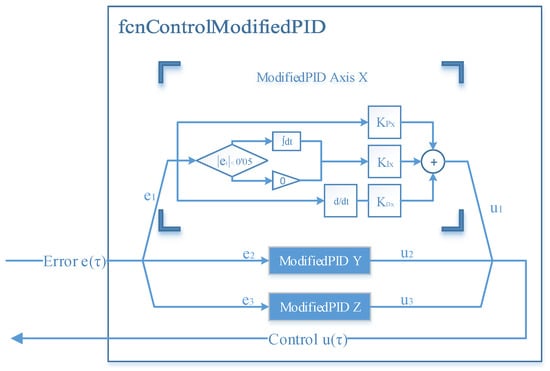
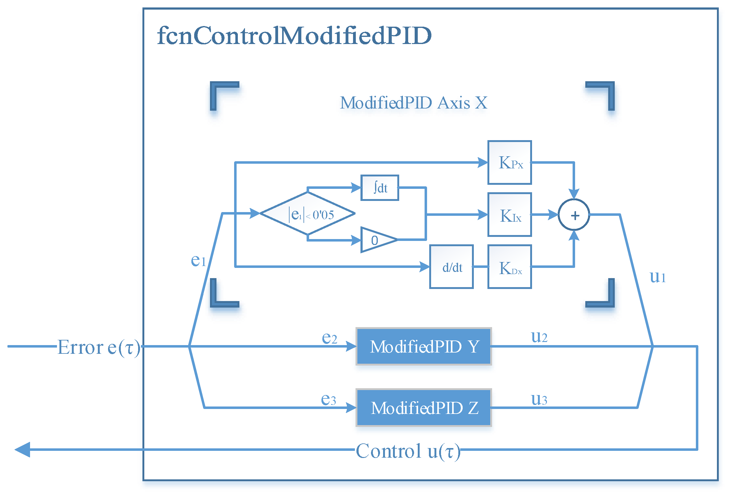
An mPID was chosen as a representative classical control theory for this study. The controller’s flow chart is shown in Figure 4.

Figure 4. mPID controller flow chart.

The input signal of the controller, $\mathit{e}\left(\tau \right)$, which consists of three components: $e_1$, $e_2$ and $e_3$, must be constructed according to the following procedure. First, the quaternion error is obtained:

$$q_e=q_{RI}\ast q_{IB}=\left[cos{\displaystyle \frac{{\theta }_e}{2}}{\mathit{n}}_{e}sin{\displaystyle \frac{{\theta }_e}{2}}\right]$$

where * denotes Hamilton product, $q_{RI}$ is the attitude of the reference frame with respect to the inertial frame, ${\theta }_e$ is the three-dimensional angular error between the two reference frames, and ${\mathit{n}}_e$ is the unit vector that defines the rotation axis. The error components along the body axes are given by the following vector:

$$\mathit{e}={\mathit{n}}_{e}sin\left({\displaystyle \frac{{\theta }_e}{2}}\right)$$

Each one of them is the orientation error between the three principal body axes (X, Y, and Z, respectively) of the satellite and their desired orientation (the reference). The output signal of the controller, u($\tau$), also consists of three components: $u_1$, $u_2$ and $u_3$. Each one is the torque actuation needed in each of the body axes to align them with the reference. The outputs are within the range [−1, +1], so they modulate the operation of the controllers from their maximum negative torque to their maximum positive torque, including the application of zero torque. In addition, the integral signal is reset every time the error signal crosses the null value. This design decision was taken because it avoids the excessive overshoot of the output signal, thus reducing the stabilization and simulation time needed for the tuning process, and because it improves the PID performance for step maneuvers.

There are three controllers (one per axis); each one of them obeys the following equation for calculating the output:

$$u_j\left(\tau \right)=K_{Pj}·e_j\left(\tau \right)+K_{Ij}·{\int }_0^{\tau }{e}_j\left(t\right)dt+K_{Dj}·{\displaystyle \frac{d{e}_j\left(\tau \right)}{d\tau }},j=1,2,3.$$

(4)

The proportional, integral, and derivative gains ($K_{Pj}$, $K_{Ij}$ and $K_{Dj}$), which result in a total of nine gains, are the tuning parameters of the mPID controllers.

3.3. Fuzzy Controller

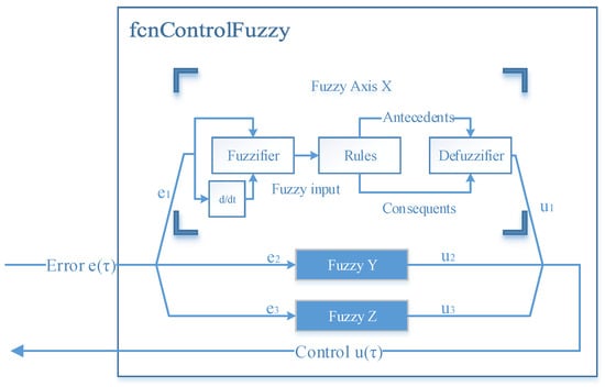
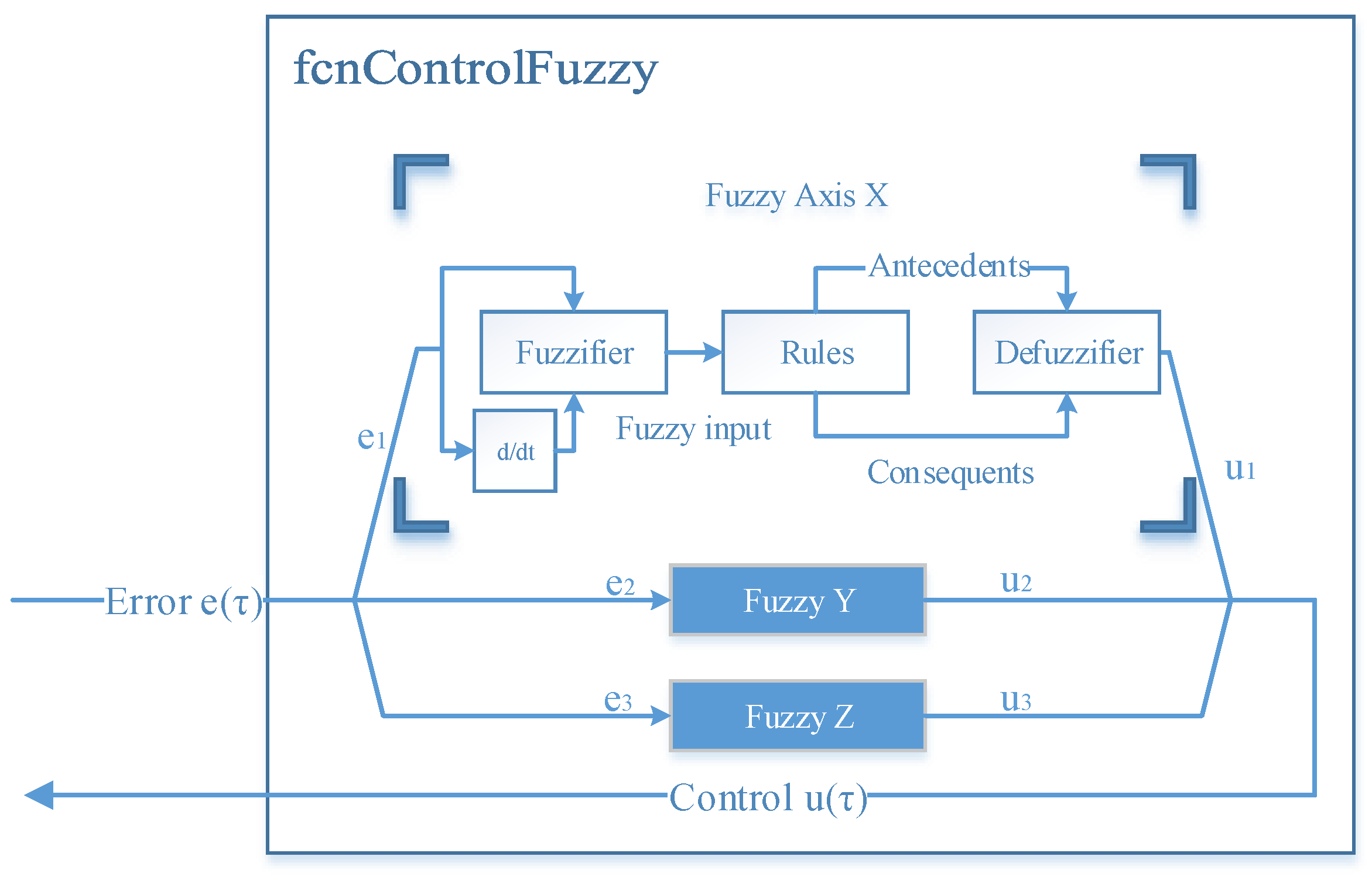
The general operation is similar to the mPID, with the same three input signals (attitude error), three controllers (one per body axis) and the same three output signals (torque actuation needed) within the range [−1, +1]. The controller’s flow chart is shown in Figure 5.

Figure 5. Fuzzy controller flow chart.

For a detailed description of the internal workings of a fuzzy controller, see [1]. The output signal calculation process can be summarized as follows:

• Fuzzification: First, the input signal and its derivative are fuzzified; transforming them into an array of values that represent the degree of membership of the input to a group of fuzzy linguistic variables: Negative Big, Negative, Negative Small, Zero, etc.
• Evaluation and aggregation of fuzzy rules: Those array values are operated and evaluated by a set of “if–then” rules, resulting in the values of the antecedents and consequents;
• Defuzzification: The output of the rules is aggregated and defuzzified using the Takagi–Sugeno method [29] which provides the discrete value of the output of the controller. As can be seen in Table 2, only five linguistic variables are used for the output.

Table 2. Selected output singleton values.

Output	NB	NS	Z	PS	PB
Maximun torque fraction	$-1$	$-0.5$	0	$0.5$	1

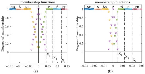
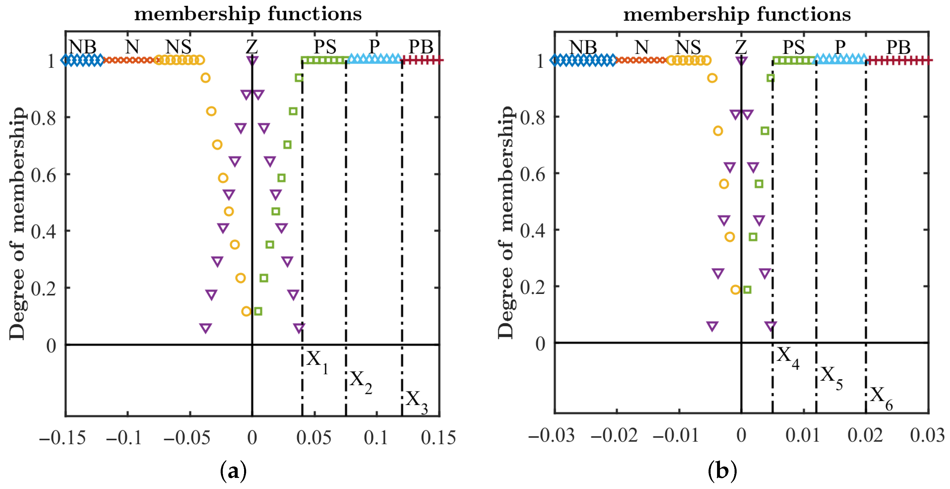
One fuzzy iteration requires quite a lot of work compared to the simple math involved in an mPID iteration. As such, the process can be tuned or adjusted by modulating many different parameters. This design modulates its performance based on six parameters per axis, $(X_1,\dots ,X_6)$, which restrict input membership functions as shown in Figure 6. Therefore, in the case of fuzzy controllers, there are 18 parameters in total that serve as the tuning parameters.

Figure 6. Input membership functions of the fuzzy controllers: NB = Negative Big, N = Negative, NS = Negative Small, Z = Zero, PS = Positive Small, etc. The “Zero” functions are triangular, and all the other ones are trapezoidal or rectangular. All are symmetric with respect to the null value, or have a conjugated one that is symmetric. All of them have an overlap with the adjacent ones of 50%, resulting in a unitary maximum value for the sum of all degrees of membership for one input. (a) Error signal input membership functions. (b) Derivative of the error signal input membership functions.

3.4. Controller Tuning Method

In order to make sure that the comparison between both controllers is reasonable, the same tuning method has been applied. It can be summarized as follows:

• First, a preliminary analysis is performed to figure out the characteristic ranges in which the crucial variables are going to exist. Also, this is a good point at which to check that the intensity of the actuators is enough to overcome the disturbance torques.
• Then, a characteristic maneuver should be selected. This maneuver has to be significant or related to the usual operation of the satellite.
• Finally, all the previous information is gathered to perform a genetic optimization.

The information from the preliminary analysis allows us to restrict the genetic search as well as to create a couple of tuning points as the initial population. The optimization aims to find multiple tuning points capable of a trade-off between the fastness and cost of the controller (a group of points forming a Pareto front), which means that there are two different and conflicting metrics evaluating the performance during a simulated maneuver.

3.4.1. Preliminary Analysis

After running a sample of simulations without actuation (free rotation simulations), it was shown that disturbance torques never exceed ${10}^{-6}$ N · m while the OPS-SAT-1 inertia wheels could generate up to ${10}^{-4}$ N · m.

Using actuation impulses, it is possible to approximate the minimum error derivative that could be introduced into the system. These approximations are summarized in Table 3.

Table 3. Approximation of the derivative inserted into the OPS-SAT-1 system with an impulse of 25 and 100 [%] of the maximum actuation when the control cycle is 0.5 s.

Impulse [%]	Axis	Min. Derivative [1/s]
	X	$7.0\times {10}^{-4}$
100	Y	$7.0\times {10}^{-4}$
	Z	$2.4\times {10}^{-3}$
	X	$1.5\times {10}^{-4}$
25	Y	$1.5\times {10}^{-4}$
	Z	$6.0\times {10}^{-4}$

Lastly, by applying the Ziegler–Nichols [30] method to the mPID controller system, it is possible to narrow down the search for the genetic algorithm domain, estimate the simulation time needed for stabilization and generate some useful tuning points as the initial population. The results of this method are summarized in Table 4.

Table 4. Results after applying the Ziegler–Nichols method to each axis.

Axis	Ultimate Gain	Oscillation Period [s]	Max. Derivative [1/s]	${\mathit{K}}_{\mathit{P}}$ Ziegler–Nichols	${\mathit{K}}_{\mathit{I}}$ Ziegler–Nichols [1/s]	${\mathit{K}}_{\mathit{D}}$ Ziegler–Nichols [s]
X	10.0	$\sim 80$	$\sim 1.8\times {10}^{-2}$	6	$\sim 1.50\times {10}^{-1}$	$\sim 6.00\times {10}^{+1}$
Y	10.0	$\sim 75$	$\sim 2.0\times {10}^{-2}$	6	$\sim 1.60\times {10}^{-1}$	$\sim 5.63\times {10}^{+1}$
Z	10.0	$\sim 45$	$\sim 3.7\times {10}^{-2}$	6	$\sim 2.67\times {10}^{-1}$	$\sim 3.38\times {10}^{+1}$

For fuzzy controllers, the first optimization starts with an initial population consisting of a pair of manually selected members: one with a lower error and the other with a lower cost. The construction of these two initial points was derived from the information obtained about the dynamics of the system during the preliminary analysis.

3.4.2. Tuning Maneuver

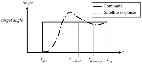
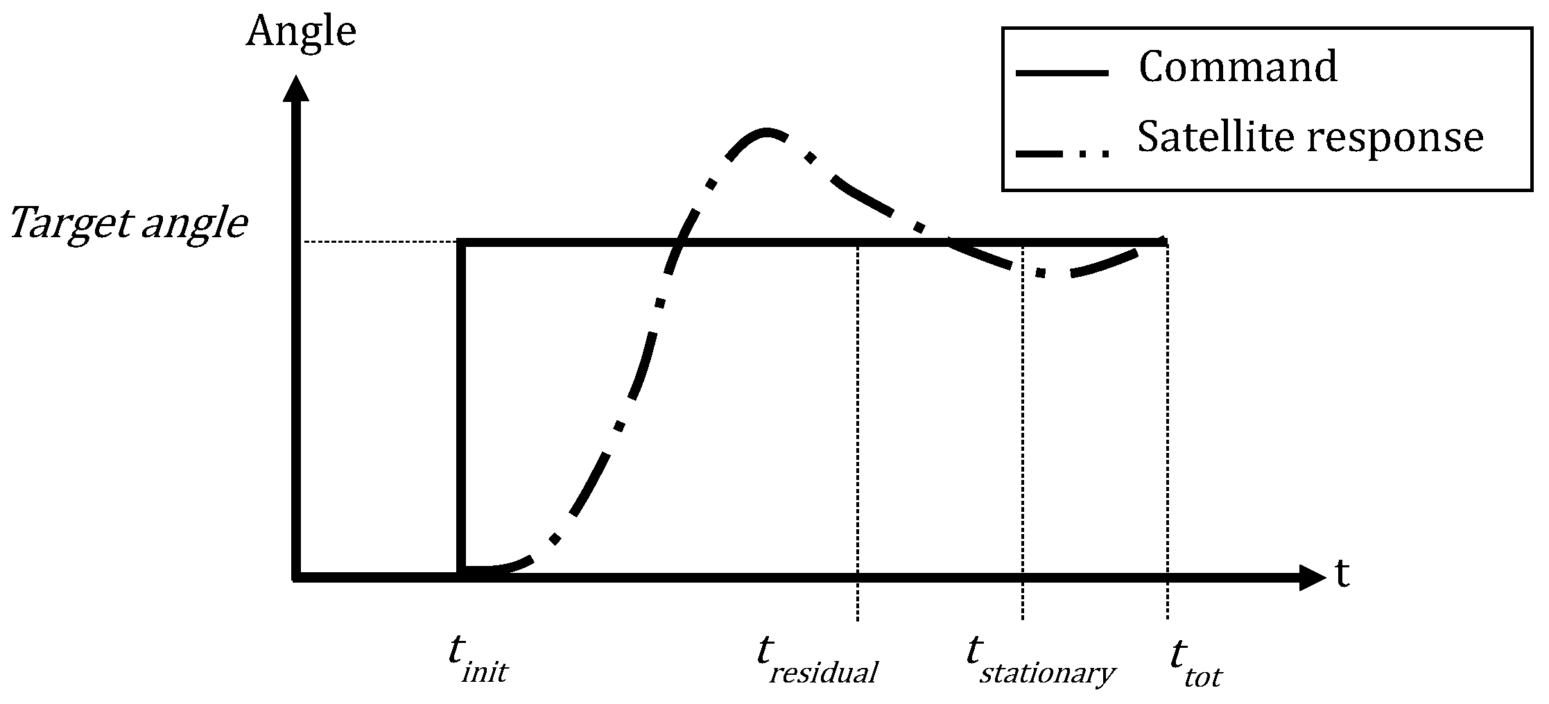
The experiment was designed such that successive step maneuvers with increasing amplitude are commanded (see Section 5), so a step command was selected as the calibration maneuver. An example of this is shown in Figure 7. As described in Section 5, the experimental campaign involves the execution of maneuvers of increasing amplitude, starting with 5° rotations and reaching up to 20°. In the final stages of the experiment, the goal is to explore the performance limits of the controller with maneuvers that exceed 30° in amplitude. For these reasons, a 20° step maneuver was selected to characterize the OPS-SAT-1 calibration maneuver. This maneuver is divided into three main phases:

Figure 7. Example of the calibration maneuver involving the orientation of one axis.

• Initial phase: The satellite begins aligned with the target axes and must maintain the angular error approximately at zero. This phase lasts 30 s and is used to evaluate initial stability metrics.
• Step phase: A 20° step is commanded around the body axis under calibration. The controller must respond accordingly to bring the satellite to the new target orientation. The duration of this phase depends on the dynamics of the specific axis and is used to evaluate the performance metrics targeted by the genetic algorithm
• Final phase: Once the target orientation is reached, the simulation continues for another 30 s, during which the controller must again maintain the angular error close to zero. This phase is used to assess residual stability metrics.

The duration of the step phase varies depending on the system’s dynamics. In the case of OPS-SAT-1, the ideal minimum durations, assuming that the actuators operate at maximum capacity throughout, with continuous acceleration during the first half of the maneuver and symmetric deceleration during the second half, without corrections, are approximately 37.5 s for the X axis, 35 s for the Y axis, and 20 s for the Z axis. These durations are used to compute the characteristic cost normalization value for the maneuver (i.e., the case where actuators operate at full capacity for the entire duration).

To allow flexibility in finding diverse controller configurations, the maximum maneuver durations are arbitrarily set to five times the ideal minimum time: 187.5 s for X, 175 s for Y, and 100 s for Z. These extended durations are used to compute the characteristic normalization value of the accumulated error in the maneuver: a controller that only reaches the target at the time limit will accumulate the maximum possible error.

3.4.3. Multi-Objective Genetic Optimization

The objective function, f, used during the tuning process, has two different and conflicting objectives: one related to fastness and the other related to cost. The specific definition of each metric is as follows:

$$f\left(1\right)={\displaystyle \frac{E}{E_{max}}},E={\int }_0^{t_{tot}}{\theta }_e\left(t\right)dt={\int }_0^{t_{tot}}2arccos{q}_{e1}\left(t\right)dt\approx 2\sum _{i=0}^{{\tau }_{tot}-1}[arccos{q}_{e1,i}+arccos{q}_{e1,i+1}]·{\displaystyle \frac{\mathrm{\Delta }{\tau }_i}{2}}$$

(5)

$$f\left(2\right)={\displaystyle \frac{C}{C_{max}}},C={\int }_0^{t_{tot}}c\left(t\right)dt\approx \sum _{i=0}^{{\tau }_{tot}-1}[{\displaystyle \frac{|T_{Cx}{|}_i+{\left|T_{Cx}\right|}_{i+1}}{|T_{Cx}{|}_{max}}}+{\displaystyle \frac{|T_{Cy}{|}_i+{\left|T_{Cy}\right|}_{i+1}}{|T_{Cy}{|}_{max}}}+{\displaystyle \frac{|T_{Cz}{|}_i+{\left|T_{Cz}\right|}_{i+1}}{|T_{Cz}{|}_{max}}}]·{\displaystyle \frac{\mathrm{\Delta }{\tau }_i}{2}}$$

(6)

where E is the accumulated error during the maneuver, which is related to the convergence time, $t_{tot}$ is the total time of the maneuver, $q_{e1}$ is the real component of the instant error quaternion (the component that accounts for the 3D angular error), ${\tau }_{tot}$ is the number of simulated step times in which the maneuver is divided, $\mathrm{\Delta }{\tau }_i$ is the step time interval, C is the accumulated cost during the maneuver, $T_{Cj}$ is the instant control torque applied in axis j, and $|T_{Cj}{|}_{max}$ is the maximum possible torque actuation in axis j.

Once the tuning parameters, the objective function, and the calibration maneuver are defined, it is time to execute the algorithm. This is performed via two main steps (see [1] for more detail):

• First, a few generations have been spent exploring the parameter domain for some candidate zones to find the optimal tuning points. For that purpose, the initial points derived from the preliminary analysis and a large population size are used, and more importance is given to the mutation mechanism.
• Finally, another optimization is performed, focusing on refining the previous results and using the settlement of the Pareto front as the stopping criterion. For that purpose, the Pareto front from the previous optimization is used as the initial population, and the population size is reduced trying to perform more generations (reducing the computational cost), giving more importance to the crossover mechanism.

4. Results

The results are to be analyzed using the performance of three characteristic points of the Pareto front: the minimum error point (ME) point; the minimum cost point (MC) point; and the central point (CP), which is the farthest point from all the extremes. Table 5 shows the values of both metrics, E and C, for the three points. The results of the optimizations for each axis are presented in the following sections.

Table 5. Optimization results for fuzzy and mPID controllers.

Point	Axis	E (Fuzzy)	E (mPID)	C (Fuzzy)	C (mPID)
ME	X	0.21	0.20	0.83	0.88
MC		1.06	0.62	0.05	0.31
CP		0.42	0.31	0.26	0.45
ME	Y	0.21	0.21	0.90	0.78
MC		0.80	0.81	0.12	0.16
CP		0.36	0.40	0.31	0.35
ME	Z	0.20	0.20	0.76	0.80
MC		0.85	0.79	0.09	0.15
CP		0.39	0.37	0.27	0.34

4.1. Performance of Controllers for Roll Axis

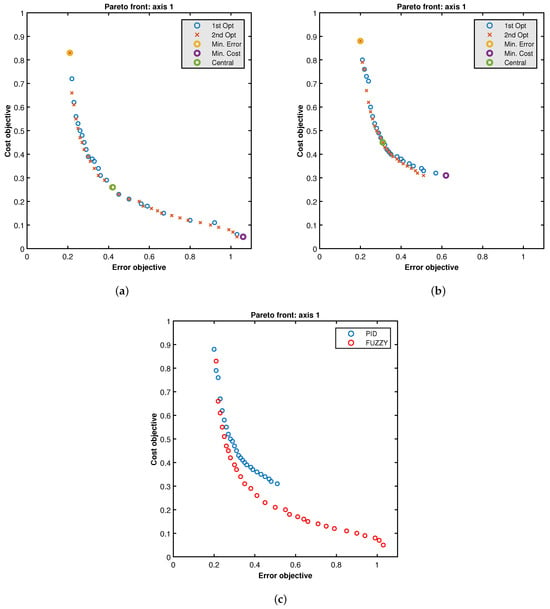
The final Pareto fronts obtained for both optimizations for each controller are shown in Figure 8. It can be seen that, for fuzzy Pareto, the first optimization was unable to identify a sufficient number of operating points in the low-cost region. In contrast, the second optimization (characterized by a high proportion of individuals generated through crossover) was able to fill the gaps in the Pareto front, significantly improving its distribution. For the mPID controller, it can be observed that the first optimization was able to identify the Pareto front, whereas the second optimization refined it.

Figure 8. X axis. (a) Fuzzy Pareto fronts for both optimizations. (b) mPID Pareto fronts for both optimizations. (c) Comparison of fuzzy and mPID Pareto fronts.

The fuzzy controller outperforms the PID controller, as its Pareto front dominates that of the PID controller, except near the ME points. The comparison of Pareto fronts shows that the performance of both controllers is similar when minimizing the first metric of the objective function (accumulated error). However, when searching for low-cost tuning points, the Pareto fronts start to split apart more and more. The tuning points found for the fuzzy controllers generally outperform the mPID ones with regard to the cost metric, meaning that they use the actuators in less time. In particular, it is possible to see that the mPID controller cannot obtain comparable low-cost tuning points. The X fuzzy controller is able to vary its accumulated error metric and its accumulated cost metric in a wide variety of configurations that allow its performance to be customized (higher convergence speed or lower cost). Specifically, as shown in Table 5, the accumulated error metric varies by approximately 80% (from 0.21 to 1.06), while the accumulated cost metric shows a variation of approximately 94% (from 0.83 to 0.05). Concerning the mPID results, the first thing that can be observed is that, despite the rigidity of the PID strategy and the fact that it is not able to reach low-cost regions, the optimization algorithm has also been able to find a wide range of operating configurations. It shows an approximately 68% variation in its error metric (from 0.20 to 0.62) and a 64% variation in its cost metric (from 0.88 to 0.31).

In Figure 9, the error and cost signals (which are directly related to the input and output signals of the controllers as well as to the objective metrics) are shown for the ME, MC and CP points. It can be seen that the fuzzy controller is capable of generating a control law (which results in the actuation profile) based on pulses that are triggered when the satellite’s dynamic state meets the appropriate conditions: an initial pulse to accelerate the system, zero actuation once the desired speed is reached, a final pulse to brake the system, and a final modulation phase to stabilize the final state.

Figure 9. Comparison of error and actuation signals for the characteristic tuning points of X axis optimization. (a) Fuzzy error. (b) Fuzzy actuation. (c) mPID error. (d) mPID actuation.

The actuation profile for the fuzzy controller corresponding to the ME point consists of two rectangular pulses (acceleration and braking, approximately of the same magnitude) and a final modulation profile (visible from approximately 60 s). These pulses are slightly separated in time; that is, there is an intermediate phase of the maneuver in which the fuzzy controller does not apply any actuation. This indicates that the genetic algorithm has not been able to find the ideal optimal operating point of the system. This phenomenon is repeated, to a greater or lesser extent, in the rest of the optimizations presented in this section. Finding this ideal point is of relatively low importance since in real situations the exact conditions of the calibration maneuver will not be reproduced. In order to approach this ideal operating point more closely, it is necessary to drastically reduce the integration step of the simulations, which increases their computational cost. In addition to the integration step, it must be taken into account that the controller computations have an operating cycle (the control cycle). This means that since most controllers do not operate in an analog manner, it will never be possible to find that operating point exactly, and it will always be necessary for there to be a gap between the pulses (a time interval in which the actuation is zero) or an overcorrection of the second pulse (because the acceleration has been too large). This latter circumstance would directly worsen the cost metric (because a greater amount of actuation is required to correct it) and indirectly worsen the error metric (because overcorrection delays the stabilization of the system).

Concerning the mPID controller, in Figure 9, it can be seen that the actuation profile of the ME point is similar to what is sought in an optimized signal: two wide pulses, one for acceleration and the next for deceleration, followed by a short modulation period to stabilize the final state. However, in the profile of the MC point, it can be seen that the actuation is never completely null, generating a signal that is extended and poorly optimized, in the sense that it lacks distinct control pulses. Transforming the PID controller into its modified variant, mPID, reduces the convergence time and therefore also decreases the area under the actuation curve (i.e., a reduction in the cost metric). However, because the way the signal is constructed makes it difficult for the control signal to reach zero at any intermediate point during the maneuver, the lowest-cost configurations are inefficient.

4.2. Performance of Controllers for Pitch Axis

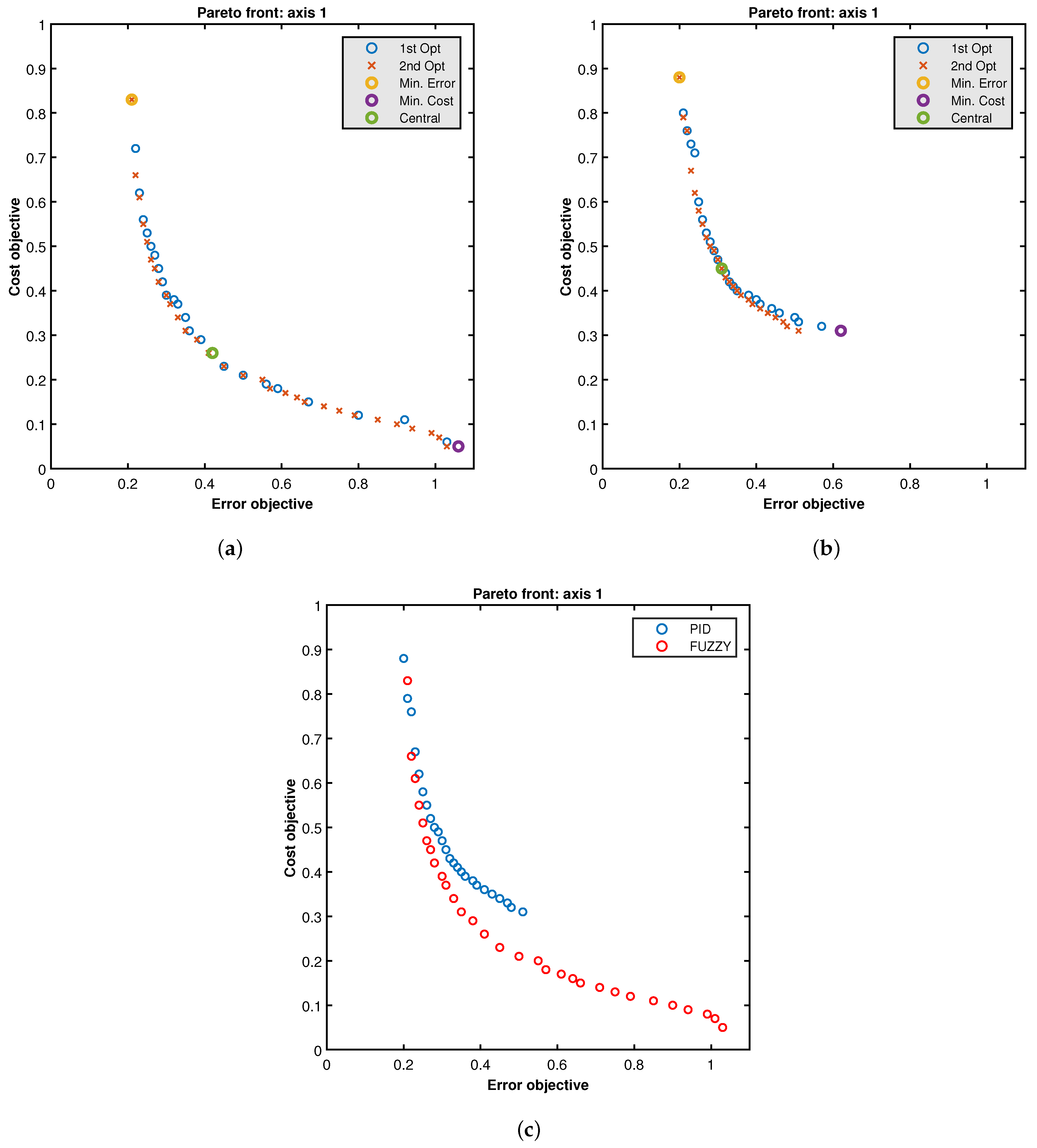
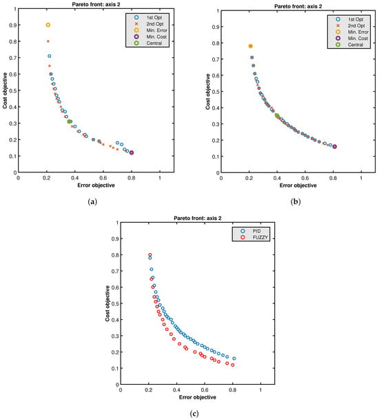
Figure 10 shows the comparison of Pareto fronts for both controllers. In a similar manner to what was discussed in the previous section, for the fuzzy Pareto front the first optimization was unable to identify a sufficient number of operating points in the low cost region. However, by means of the crossover mechanism, the second optimization succeeded in improving its overall dispersion. For the mPID, the first optimization succeeded in identifying a part of the Pareto front; however, the distribution remains suboptimal, particularly in the low-cost region. The second optimization did not achieve any significant improvement over the results obtained in the first stage.

Figure 10. Y axis. (a) Fuzzy Pareto fronts for both optimizations. (b) mPID Pareto fronts for both optimizations. (c) Comparison of fuzzy and mPID Pareto fronts.

The fuzzy controller outperforms the PID controller, as its Pareto front dominates that of the PID controller, except near the ME points. In this case, the small distance between the fronts is emphasized. Moreover, note that along this axis the mPID controller is able to expand the low-cost region by extending the front, although with a higher cost than the fuzzy one. Specifically, as shown in Table 5, the fuzzy controller Y is capable of varying its accumulated error metric by approximately 74% (from 0.21 to 0.80) and its accumulated cost metric by approximately 87% (from 0.90 to 0.12). Concerning the mPID controller, it is able to vary its error metric by approximately 74% (from 0.21 to 0.81) and its cost metric by approximately 76% (from 0.76 to 0.18).

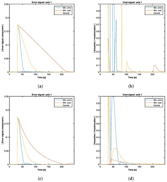
In Figure 11, the error and cost signals are shown for the ME, MC and CP points. As expected, the fuzzy Y controller was able to reproduce the desired behavior through control impulses. Observing the mPID signal profiles, a behavior similar to that observed for the X axis can be identified. However, the actuation profile of the minimum-cost point is noticeably different because the dynamics of the Y axis requires a smaller initial impulse to reach stabilization conditions in time. As a result, by definition, the cost metrics achievable by this controller are lower than those of the X axis.

Figure 11. Comparison of error and actuation signals for the characteristic tuning points of Y axis optimization. (a) Fuzzy error. (b) Fuzzy actuation. (c) mPID error. (d) mPID actuation.

4.3. Performance of Controllers for Yaw Axis

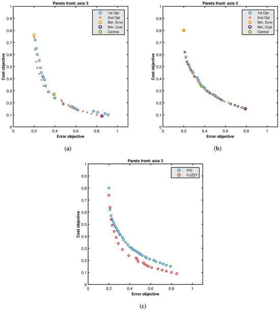
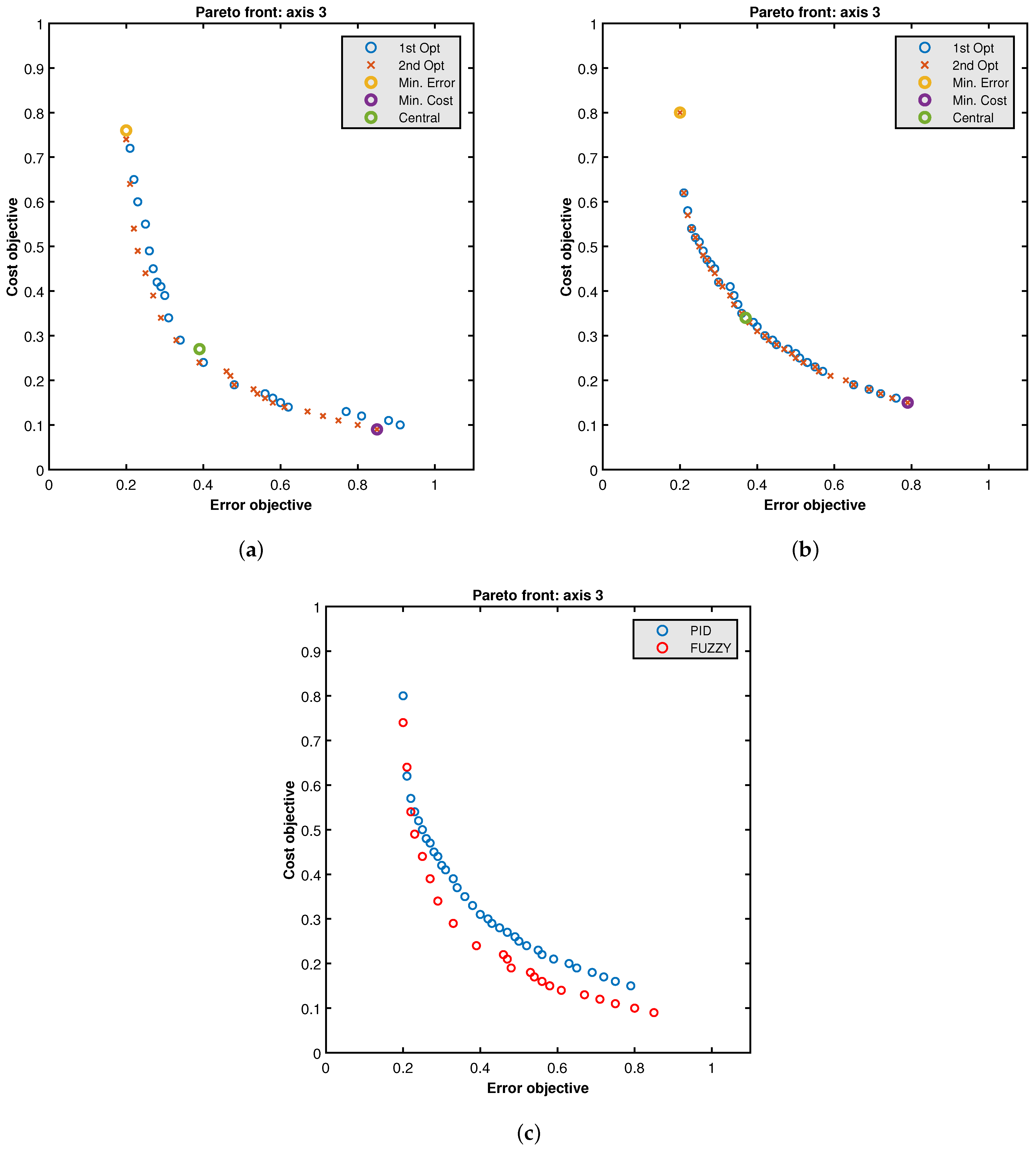
Figure 12 shows the comparison of Pareto fronts for both controllers. The behavior is similar to that of the Y axis, although in this case the fuzzy Pareto front fully dominates that of the PID controller. As in the other axes, a wide range of design points has been found. The fuzzy Z controller can vary its error by 76% (from 0.20 to 0.85) and its cost by 88% (from 0.76 to 0.09). Concerning mPID, the Z controller can vary its error by 75% (from 0.20 to 0.79) and its cost by 81% (from 0.80 to 0.15).

Figure 12. Z axis. (a) Fuzzy Pareto fronts for both optimizations. (b) mPID Pareto fronts for both optimizations. (c) Comparison of fuzzy and mPID Pareto fronts.

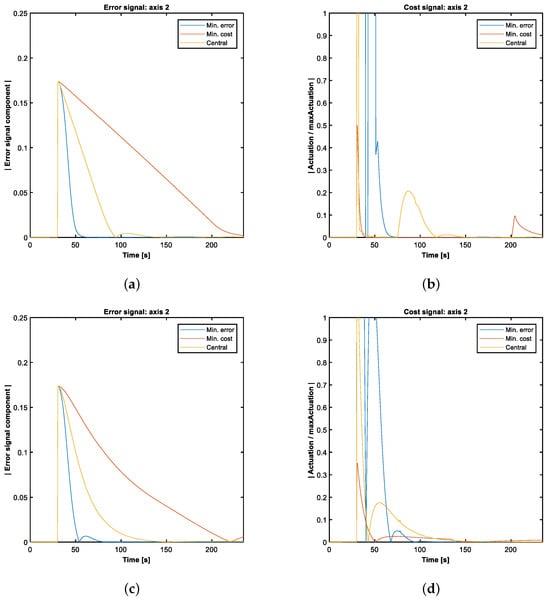
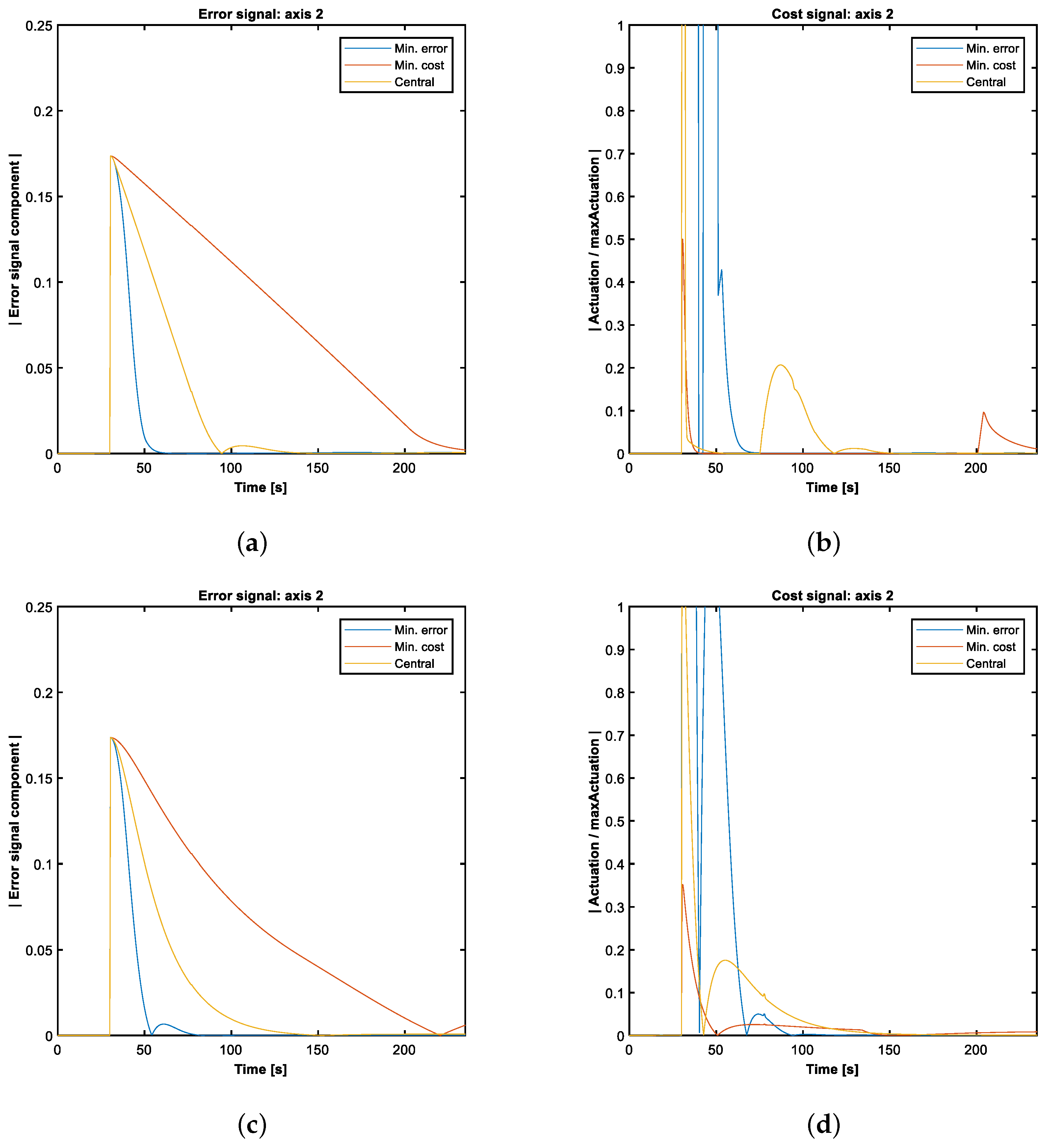
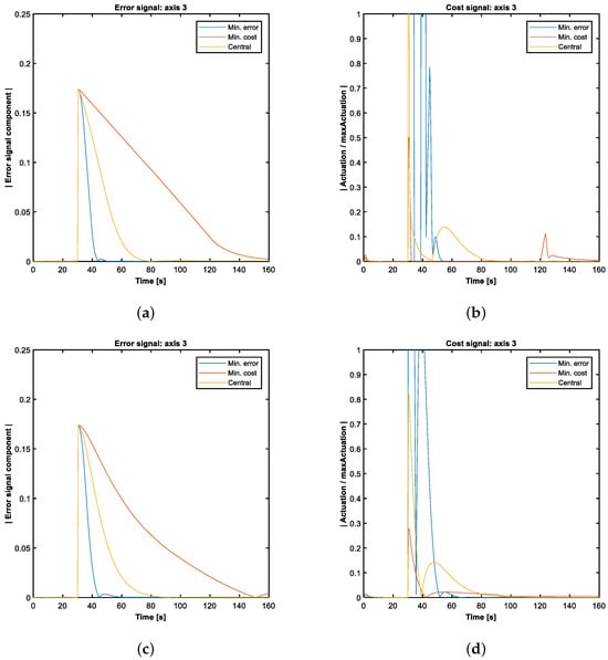
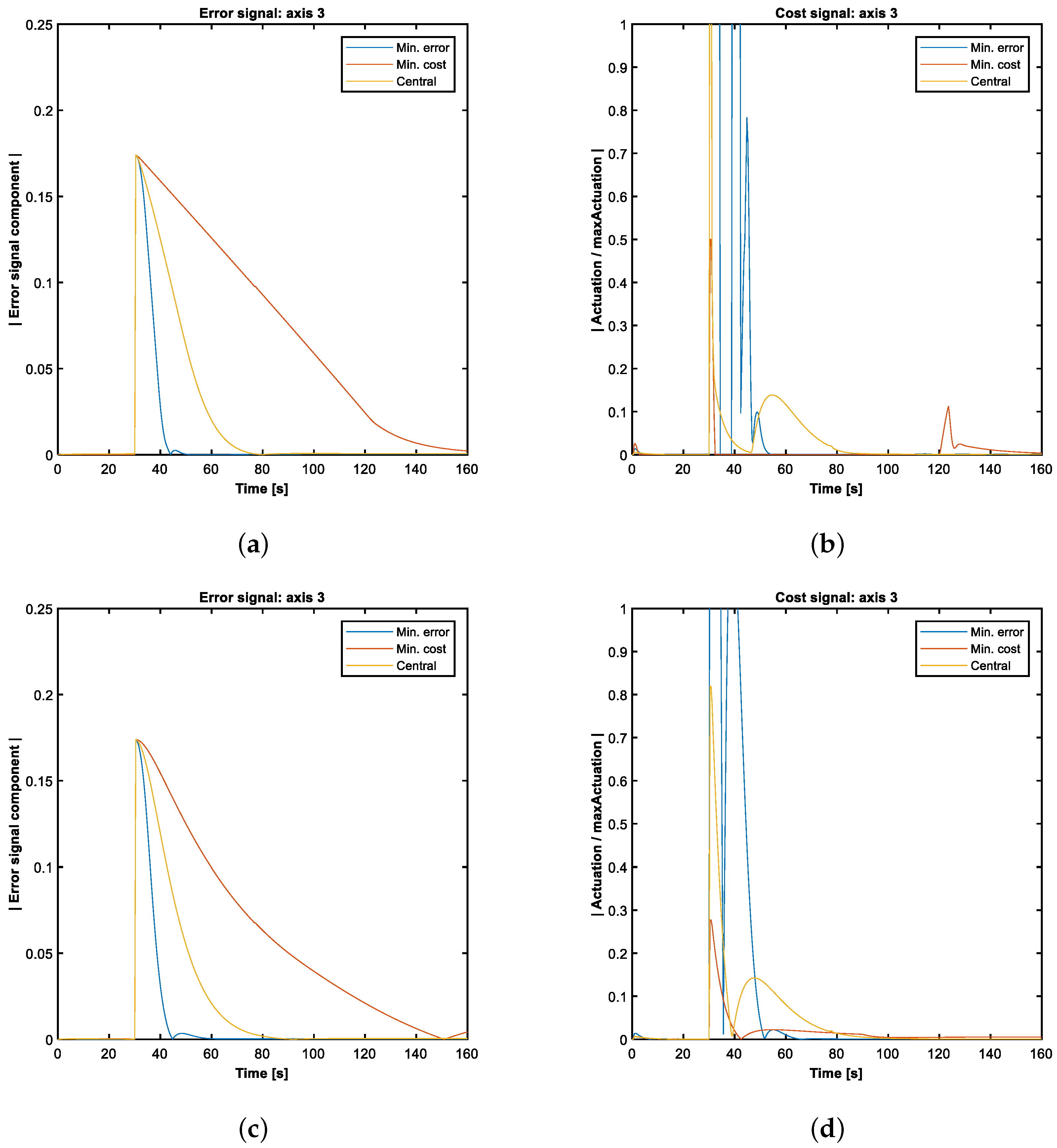
In Figure 13 the error and cost signals are shown for the ME, MC and CP points. When comparing the dynamics of the pitch axis with those of the yaw axis, a noticeable difference in the stabilization times can be observed: the dynamics of the Z axis are the most agile in the system, mainly because the moment of inertia of OPS-SAT-1 is significantly smaller along this axis.

Figure 13. Comparison of error and actuation signals for the characteristic tuning points of Z axis optimization. (a) Fuzzy error. (b) Fuzzy actuation. (c) mPID error. (d) mPID actuation.

4.4. Monte Carlo Analysis

To evaluate the robustness of the mPID and fuzzy control strategies against parameter uncertainties, a Monte Carlo analysis was conducted.

In the simulations, the initial parameters subject to variation comprise both the orbital characteristics and the intrinsic properties of the satellite. The OPS-SAT-1 followed a circular heliocentric orbit; consequently, the initial eccentricity and inclination parameters are fixed at 0° and 97.4779°, respectively, as both remained largely unchanged throughout the operational lifetime of OPS-SAT-1. The Right Ascension of the Ascending Node (RAAN) is modeled as a uniformly distributed random variable throughout the interval [0°, 360°]. The altitude is modeled as another uniform distribution that spans from the initial altitude of the satellite (515 km) to the altitude at which the mission ended (400 km). In the simulations, the initial orbit is assumed to be circular; therefore, the argument of perigee is treated as located at the ascending node. The full range of possible scenarios is addressed by modeling the true anomaly as a uniformly distributed variable over the interval [0°, 360°]. The OPS-SAT-1 attitude controllers were designed to maintain the spacecraft’s orientation using reaction wheels and to allow maneuvers within the operational range of these actuators. Consequently, the initial condition is assumed to be zero angular velocity with respect to the orbital axes, while initial attitude errors of ±20° per axis are considered. A larger deviation would saturate the angular momentum storage capacity of the reaction wheels.

Regarding the intrinsic properties of the satellite (see Table 1), they are defined according to its ICD [31], where nominal values are provided and a 5% margin is advised. However, in order to achieve a more precise analysis of the dependence of the error, the steady-state error, and the cost on the moments of inertia, a threefold margin will be considered, namely 15%. For the products of inertia, since their magnitude is at most two orders lower than that of the principal moments of inertia, and given that the dependence of the performance metrics on these terms has already been analyzed in previous works where no correlation was observed [1,24], only their nominal value will be considered.

Finally, an internal satellite error is considered, whereby the torque actually applied does not exactly match the commanded one. This simulates actuator calibration errors, misalignments, and similar effects. This error has been modeled as a uniformly distributed random variable within $\pm 20\%$ of the maximum wheel torque.

A summary of all the parameters varied in the Monte Carlo analysis, together with the ranges considered, can be found in Table 6.

Table 6. Monte Carlo parameters.

Type	Parameter	Range
Orbit	Altitude	[400, 515] km
	Ecc	0
	Inc	97.4779°
	RAAN	[0°, 360°]
	Argument of periapsis	0°
	True Anomaly	[0°, 360°]
Initial Attitude error	Yaw	[−20°, 20°]
	Pitch	[−20°, 20°]
	Roll	[−20°, 20°]
Spacecraft parameters	$I_{xx}$	0.06577296 $\pm 15\%$
	$I_{yy}$	0.05647602 $\pm 15\%$
	$I_{zz}$	0.01650073 $\pm 15\%$
	Comanding error	$\pm 20\%$

A total of 8000 simulations were performed, with each controller operating at a frequency of 5 Hz. In optimization procedures, when commanding maneuvers were performed on a single axis, only the errors and costs associated with that axis were evaluated. However, for the Monte Carlo analysis, a metric related to the attitude error in three axes is used: the arctangent of the ratio between the Euclidean norm of the error quaternion’s vector part, ${\mathbf{q}}_e$, and the absolute value of its scalar part, $q_{0e}$, as defined in Equation (7), instead of ${\theta }_e$, in order to avoid numerical issues related to the arcsine and the arccosine.

$${\beta }_e\left(t\right)=2arctan\left({\displaystyle \frac{\parallel {\mathbf{q}}_e\left(t\right)\parallel }{|q_{0e}\left(t\right)|}}\right).$$

(7)

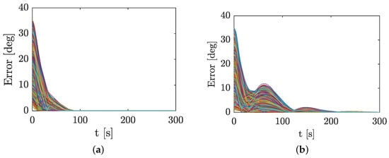
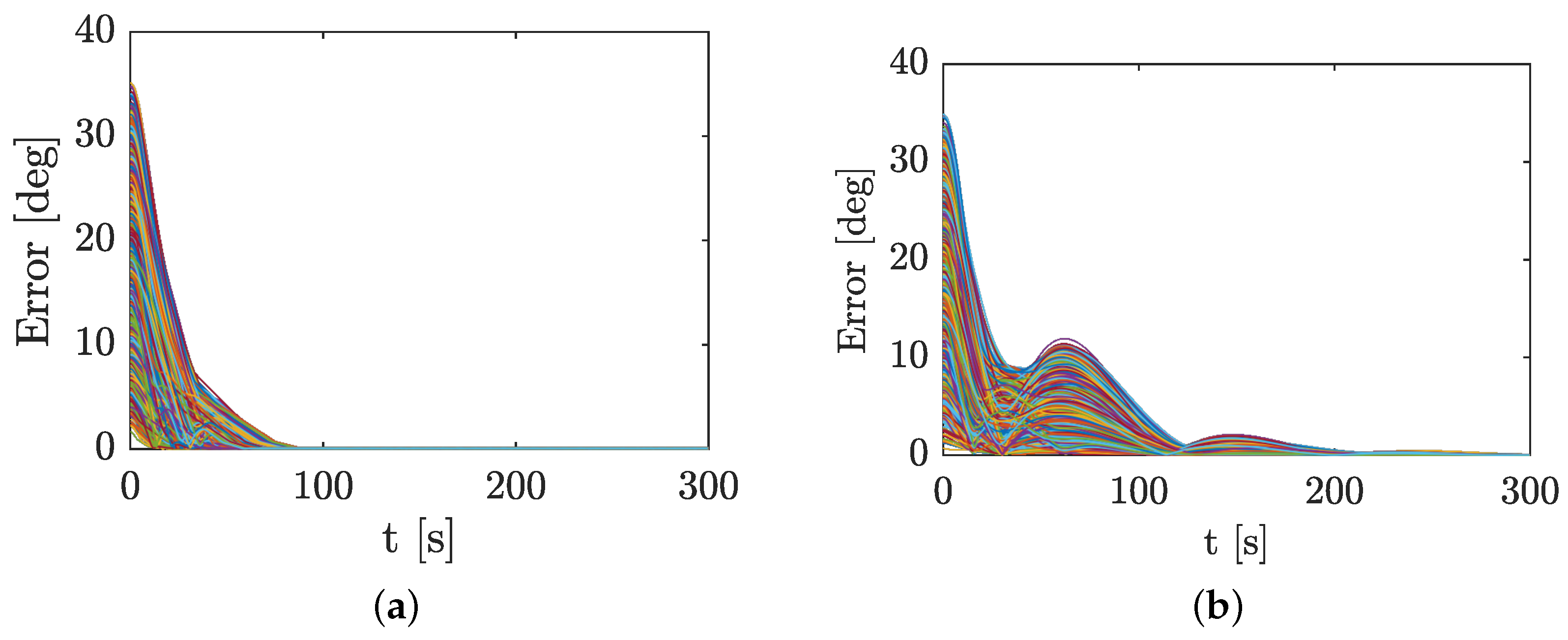
To illustrate the behavior of the controllers under Monte Carlo parameter uncertainties, Figure 14 presents the time evolution of the error signals of the fuzzy and mPID controllers for the CPs of the Pareto fronts. It can be observed that, for the fuzzy controller, all simulations converge in less than 100 s. In the case of the mPID controller, both the convergence time and the steady-state error are greater than those of the fuzzy controller. In addition, the error profiles exhibit overshoot.

Figure 14. Error signals for CP. (a) Fuzzy; (b) mPID. Each line corresponds to one of the 8000 simulations.

The results of the Monte Carlo analysis are summarized in Table 7. The accumulated error is defined as the integral of ${\beta }_e\left(t\right)$ (Equation (7)) divided by the duration of the maneuver (300 s). The settling time is defined as the time required for the error signal ${\beta }_e\left(t\right)$ to reach 0.1 rad without subsequently exceeding that value. The steady-state error is defined as the integral of ${\beta }_e\left(t\right)$ over the last minute, divided by the integration time (60 s). Finally, the accumulated cost is defined as the integral of the norm of the angular velocity vector of the reaction wheel, normalized with respect to maintaining one wheel at its maximum acceleration for one minute.

Table 7. Monte Carlo results (mean values).

	Accumulated Error [rad]	Settling Time [s]	Steady-State Error [rad]	Accumulated Cost
Fuzzy CP	1.2193	55.8407	0.0557	0.6264
PID CP	2.3085	242.6322	0.0736	0.4780

As can be observed, on average, for the central controller, the PID control law exhibits 89% more accumulated error, requires 335% more time to converge to an error below 0.1 rad, and its steady-state error during the final minute of a 5 min maneuver is 32% higher. However, it is observed that when an error is introduced into the command signal, the PID controller yields a 24% lower cost. This is an expected result, since the advantage of the fuzzy controller lies in its ability to perform the maneuver through two main pulses (acceleration and braking), with a constant velocity phase between them. However, when an error is introduced in the command signal, this phase becomes altered as the torque is no longer exactly zero. Although an error around 20% of the maximum torque in the command signal would be considered unacceptable for a space mission, it nevertheless highlights the sensitivity of these controllers to this type of error. Consequently, the need to implement methodologies that mitigate this effect should be examined, as suggested in [32].

5. Experiment Protocol

To take advantage of this unique opportunity, an experimental campaign was designed to include a comprehensive set of simple attitude maneuvers—specifically step commands. The use of simple single-axis maneuvers minimizes complex dynamic interactions, such as coupled rotations across multiple axes. This simplification allows for a clearer distinction between the effects generated by the actuators (controlled and desired) and those produced by environmental disturbances (uncontrolled, undesired, and often difficult to model).

Each maneuver is executed using both the mPID controller and the fuzzy one, allowing a direct experimental comparison under nearly identical conditions. Furthermore, identical maneuvers are planned around different body axes, which helps analyze the modeling accuracy of external disturbances and assess whether their effects are consistent across rotational dynamics along all axes.

The complete experimental plan is structured into five descending priority levels (from #1 to #5), allowing the operations team to cancel, shorten or postpone lower-priority segments if unforeseen time constraints arise. Each priority group contains nine experiments that can be executed modularly or consecutively. Consecutive execution is recommended to minimize the variations in disturbance torques and improve the post-processing accuracy by simplifying the separation of controlled and perturbative effects. Table 8 shows level #1, as an example.

Table 8. Experiment protocol.

Priority	Exp #	Man #	Controller	Quaternion Objective				Angle Objective [deg]			Time [s]
				${\mathit{q}}_{\mathbf{0}}$	${\mathit{q}}_{\mathbf{1}}$	${\mathit{q}}_{\mathbf{2}}$	${\mathit{q}}_{\mathbf{3}}$	Roll	Pitch	Yaw
1	1	0	Default	1	0	0	0	0	0	0	300
		1	FUZZY-CP	0.999	0.044	0	0	5	0	0
		2	FUZZY-CP	1	0	0	0	0	0	0
		3	PID-CP	0.999	0.044	0	0	5	0	0
		4	PID-CP	1	0	0	0	0	0	0
		5	FUZZY-CP	0.999	−0.044	0	0	−5	0	0
		6	FUZZY-CP	1	0	0	0	0	0	0
		7	PID-CP	0.999	−0.044	0	0	−5	0	0
		8	PID-CP	1	0	0	0	0	0	0
	2	The same procedure as in experiment #1, but with the command on the Y axis (pitch angle).
	3	The same procedure as in experiment #1, but with the command on the Z axis (yaw angle).
	4	0	Default	1	0	0	0	0	0	0	300
		1	FUZZY-CP	0.996	0.087	0	0	10	0	0
		2	FUZZY-CP	1	0	0	0	0	0	0
		3	PID-CP	0.996	0.087	0	0	10	0	0
		4	PID-CP	1	0	0	0	0	0	0
		5	FUZZY-CP	0.996	−0.087	0	0	−10	0	0
		6	FUZZY-CP	1	0	0	0	0	0	0
		7	PID-CP	0.996	−0.087	0	0	−10	0	0
		8	PID-CP	1	0	0	0	0	0	0
	5	The same procedure as in experiment #4, but with the command on the Y axis (pitch angle).
	6	The same procedure as in experiment #4, but with the command on the Z axis (yaw angle).
	7	Same as in #1 (same sequence as in #4, #5, and #6), but with commands of 15° amplitude.
	8	Same as in #2 (same sequence as in #4, #5, and #6), but with commands of 15° amplitude.
	9	Same as in #3 (same sequence as in #4, #5, and #6), but with commands of 15° amplitude.
2	The same procedure as in priority #1 but using the low-cost variants (FUZZY-LC and PID-LC).
3	The same procedure as in priority #1 but using the low-error variants (FUZZY-LE and PID-LE).

Each experiment consists of eight step maneuvers, defined by the control strategy used, the calibration parameters applied, and the specific target attitude. Maneuvers are grouped in pairs: for every commanded rotation, a subsequent maneuver of equal amplitude and opposite direction returns the satellite to its nominal attitude. Before each experiment, a default controller is engaged (see Section 3.1). This procedure ensures that initial conditions—both in terms of the attitude error and actuator availability—are consistent and comparable across all experiments.

Three different operating points are tested on the Pareto front: LC, LE and CP. Each maneuver essentially represents a small step command, increasing in angular amplitude by increments of 5° or 10°, up to a maximum of 40°, to avoid the excessive shadowing of the main solar array and thus prevent critical power loss. A time limit of 300 s is allocated per maneuver. If a maneuver fails to complete within this time, the sequence proceeds to the next command without aborting the experiment; the failure will be diagnosed during post-analysis. If completed ahead of time, the controller is expected to maintain the achieved target attitude for the remainder of the 300 s.

6. Discussion

This study presents the design and implementation of an attitude control experiment on the OPS-SAT-1 platform, with the primary objective of advancing the field of satellite attitude control through the demonstration of intelligent control strategies, particularly fuzzy logic controllers. The deployment of these algorithms in an operational space environment enables the identification and mitigation of hardware and system-level challenges that are typically absent in simulation-based analysis. In fact, due to technical problems in communication with the OPS-SAT-1 hardware, the experiment could not be conducted in orbit, and only the numerical results could be analyzed.

The optimization results provide further empirical evidence supporting the superior performance of modern control techniques compared to classical methods. As suggested in previous research, fuzzy control strategies exhibit notable advantages, particularly in scenarios that require energy-efficient performance. The incorporation of genetic algorithms for tuning further underscores the flexibility of the proposed methodology, allowing the controller architecture to adapt to diverse mission scenarios and operational constraints. The robustness analysis shows that, although the energy cost of the maneuver may worsen if there is a significant error in the control signal, the fuzzy controller still maintains better metrics in accumulated error, steady-state error, and settling time.

The modular structure of the control system—featuring configurable membership functions and rule sets—proved especially suitable for a range of mission phases, from initial detumbling operations to high-precision science-pointing maneuvers. This adaptability highlights the potentially broad applicability of the proposed control framework to future missions with varying objectives and requirements.

Furthermore, the controller architecture, the simulation environment, and the optimization methodology developed in this work constitute a reusable framework that can be applied to other mission contexts. The generalist nature of the tuning approach, combined with the efficiency of evolutionary optimization algorithms, facilitates the exploration of a wide range of control trade-offs, balancing response time and power consumption.

Overall, this work contributes to the design of ADCS for small satellites, offering insights into the trade-offs and benefits of integrating intelligent control techniques. Although PID controllers remain a reliable benchmark, the integration of fuzzy logic introduces benefits in terms of adaptability and energy efficiency.

References

- Bello, Á. Parameterized fuzzy-logic controllers for the attitude control of nanosatellites in low Earth orbits. A comparative studio with PID controllers. Expert Syst. Appl. 2021, 174, 114679. [Google Scholar] [CrossRef] [Scilit]
- de Souza, L.C.G. Design of Satellite Control System Using Optimal Nonlinear Theory. Mech. Based Des. Struct. Mach. 2006, 34, 351–364. [Google Scholar] [CrossRef] [Scilit]
- Liu, H.; Guo, L.; Zhang, Y. An anti-disturbance PD control scheme for attitude control and stabilization of flexible spacecrafts. Nonlinear Dyn. 2012, 67, 2081–2088. [Google Scholar] [CrossRef] [Scilit]
- Sidi, M.J. Spacecraft Dynamics and Control: A Practical Engineering Approach; Cambridge University Press: Cambridge, UK, 2014. [Google Scholar] [CrossRef] [Scilit]
- Souza, A.G.; Souza, L.C.G. Design of a controller for a rigid-flexible satellite using the H-infinity method considering the parametric uncertainty. Mech. Syst. Signal Process. 2019, 116, 641–650. [Google Scholar] [CrossRef] [Scilit]
- Eshghi, S.; Varatharajoo, R. Nonsingular terminal sliding mode control technique for attitude tracking problem of a small satellite with combined energy and attitude control system (CEACS). Aerosp. Sci. Technol. 2018, 76, 14–26. [Google Scholar] [CrossRef] [Scilit]
- Banerjee, A.; Amrr, S.M.; Nabi, M. A pseudospectral method based robust-optimal attitude control strategy for spacecraft. Adv. Space Res. 2019, 64, 1688–1700. [Google Scholar] [CrossRef] [Scilit]
- Hegrenæs, Ø.; Gravdahl, J.T.; Tøndel, P. Spacecraft attitude control using explicit model predictive control. Automatica 2005, 41, 2107–2114. [Google Scholar] [CrossRef] [Scilit]
- Altan, A.; Hacıoğlu, R. Model predictive control of three-axis gimbal system mounted on UAV for real-time target tracking under external disturbances. Mech. Syst. Signal Process. 2020, 138, 106548. [Google Scholar] [CrossRef] [Scilit]
- Murilo, A.; de Deus Peixoto, P.J.; de Souza, L.C.G.; Lopes, R.V. Real-time implementation of a parameterized Model Predictive Control for Attitude Control Systems of rigid-flexible satellite. Mech. Syst. Signal Process. 2021, 149, 107129. [Google Scholar] [CrossRef] [Scilit]
- Rodrigues, R.; Murilo, A.; Lopes, R.V.; Souza, L.C.G.D. Hardware in the Loop Simulation for Model Predictive Control Applied to Satellite Attitude Control. IEEE Access 2019, 7, 157401–157416. [Google Scholar] [CrossRef] [Scilit]
- Guan, P.; Liu, X.-J.; Liu, J.-Z. Adaptive fuzzy sliding mode control for flexible satellite. Eng. Appl. Artif. Intell. 2005, 18, 451–459. [Google Scholar] [CrossRef] [Scilit]
- Cheng, C.-H.; Shu, S.-L.; Cheng, P.-J. Attitude control of a satellite using fuzzy controllers. Expert Syst. Appl. 2009, 36, 6613–6620. [Google Scholar] [CrossRef] [Scilit]
- Kim, S.-W.; Park, S.-Y.; Park, C. Spacecraft attitude control using neuro-fuzzy approximation of the optimal controllers. Adv. Space Res. 2016, 57, 137–152. [Google Scholar] [CrossRef] [Scilit]
- Chen, Z.; Zhong, L.; Liu, X.; Cong, B. Adaptive Fuzzy PD+ Control for Attitude Maneuver of Rigid Spacecraft. Asian J. Control 2016, 18, 631–641. [Google Scholar] [CrossRef] [Scilit]
- Chak, Y.-C.; Varatharajoo, R.; Razoumny, Y. Disturbance observer-based fuzzy control for flexible spacecraft combined attitude & sun tracking system. Acta Astronaut. 2017, 133, 302–310. [Google Scholar] [CrossRef] [Scilit]
- Najafizadeh Sari, N.; Jahanshahi, H.; Fakoor, M. Adaptive Fuzzy PID Control Strategy for Spacecraft Attitude Control. Int. J. Fuzzy Syst. 2019, 21, 769–781. [Google Scholar] [CrossRef] [Scilit]
- Li, A.; Liu, M.; Shi, Y. Adaptive sliding mode attitude tracking control for flexible spacecraft systems based on the Takagi-Sugeno fuzzy modelling method. Acta Astronaut. 2020, 175, 570–581. [Google Scholar] [CrossRef] [Scilit]
- Zou, A.-M.; Kumar, K.D.; Hou, Z.-G. Quaternion-Based Adaptive Output Feedback Attitude Control of Spacecraft Using Chebyshev Neural Networks. IEEE Trans. Neural Netw. 2010, 21, 1457–1471. [Google Scholar] [CrossRef] [Scilit]
- Fazlyab, A.R.; Saberi, F.F.; Kabganian, M. Adaptive attitude controller for a satellite based on neural network in the presence of unknown external disturbances and actuator faults. Adv. Space Res. 2016, 57, 367–377. [Google Scholar] [CrossRef] [Scilit]
- Yadava, D.; Hosangadi, R.; Krishna, S.; Paliwal, P.; Jain, A. Attitude control of a nanosatellite system using reinforcement learning and neural networks. In Proceedings of the 2018 IEEE Aerospace Conference, Big Sky, MT, USA, 3–10 March 2018; IEEE: Big Sky, MT, USA, 2018; pp. 1–8. [Google Scholar] [CrossRef] [Scilit]
- Zadeh1965 Zadeh, L.A. Fuzzy Sets. Inf. Control 1965, 8, 338–353. [Google Scholar] [CrossRef] [Scilit]
- Walker, A.R.; Putman, P.T.; Cohen, K. Solely Magnetic Genetic/Fuzzy-Attitude-Control Algorithm for a CubeSat. J. Spacecr. Rocket. 2015, 52, 1627–1639. [Google Scholar] [CrossRef] [Scilit]
- Calvo, D.; Avilés, T.; Lapuerta, V.; Laverón-Simavilla, A. Fuzzy attitude control for a nanosatellite in low Earth orbit. Expert Syst. Appl. 2016, 58, 102–118. [Google Scholar] [CrossRef] [Scilit]
- Mukherjee, B.K.; Giri, D.K.; Sinha, M. Lorentz-Force-Based Fuzzy Proportional–Integral–Derivative Attitude Control for Earth-Pointing Satellites. J. Spacecr. Rocket. 2017, 54, 1153–1160. [Google Scholar] [CrossRef] [Scilit]
- Ahmed, H.H.A.; Mashor, M.Y.; Mahdi, M.C. Intelligent Fuzzy PD+I Controller with Stabilizer for Nano Satellite Attitude Control System. J. Phys. Conf. Ser. 2019, 1372, 012022. [Google Scholar] [CrossRef] [Scilit]
- Olfe, K.; Ezquerro, J.M.; Rodríguez, J.; Arshadi, A.; Laverón-Simavilla, A.; Lapuerta, V. Attitude control experiment design for OPS-SAT Missions. IEEE Aerosp. Electron. Syst. Mag. 2026. [Google Scholar] [CrossRef] [Scilit]
- European Space Agency. OPS-SAT. Available online: https://opssat.esa.int/ (accessed on 1 March 2026).
- Takagi, T. Fuzzy Identification of Systems and Its Applications to Modeling and Control. IEEE Trans. Syst. Man Cybern. 1985, SMC-15, 116–132. [Google Scholar] [CrossRef] [Scilit]
- Ziegler, J.G. Optimum settings for automatic controllers. J. Dyn. Syst. Meas. Control 1993, 115, 759–765. [Google Scholar] [CrossRef] [Scilit]
- Henkel, M.; Romano, P.; Zeif, R. OPS-SAT Phase B2/C/D/E1: Experimenter ICD; Contract nr: TUG/ESA/OPS-SAT/EICD/4000113614/15/D/SR; Graz University of Technology: Graz, Austria, 2016. [Google Scholar]
- Olfe, K.; Bello, A.; Fernández, J.; Rodríguez, J.; Lapuerta, V. Design and experimental verification of a robust control to avoid individual calibration of multiple reaction wheels in satellites. Adv. Space Res. 2025, 75, 767–778. [Google Scholar] [CrossRef] [Scilit]
Disclaimer/Publisher’s Note: The statements, opinions and data contained in all publications are solely those of the individual author(s) and contributor(s) and not of MDPI and/or the editor(s). MDPI and/or the editor(s) disclaim responsibility for any injury to people or property resulting from any ideas, methods, instructions or products referred to in the content. |
© 2026 by the authors. Licensee MDPI, Basel, Switzerland. This article is an open access article distributed under the terms and conditions of the Creative Commons Attribution (CC BY) license.