Transient Modeling and Analysis of Short-Circuit Faults in the DC Power System for Hybrid Electric Aircraft

Abstract

Transient modeling of short-circuit faults in the DC power system of hybrid electric aircraft (HEA) serves as a fundamental basis for effective fault identification, localization, and isolation. Before faults are detected and protective measures are taken, distributed sources and loads maintain their normal control strategies. However, previous studies frequently overlook the impact of these control dynamics on the transient behavior of DC power systems, leading to reduced accuracy in fault transient models. Therefore, this paper proposes a fault transient modeling method for the DC power system of HEA considering the control effects of distributed sources and loads. Firstly, the transient characteristics of all components in the system are analyzed, including generators and fan motors, batteries and DC load, and supercapacitors. Subsequently, a comprehensive fault transient model of the HEA DC power system is established. Finally, the validity of the proposed method is verified through comparison with results from a semi-physical test platform. The results demonstrate that the proposed modeling approach enhances the accuracy of transient analysis for the faulty HEA DC power systems.

1. Introduction

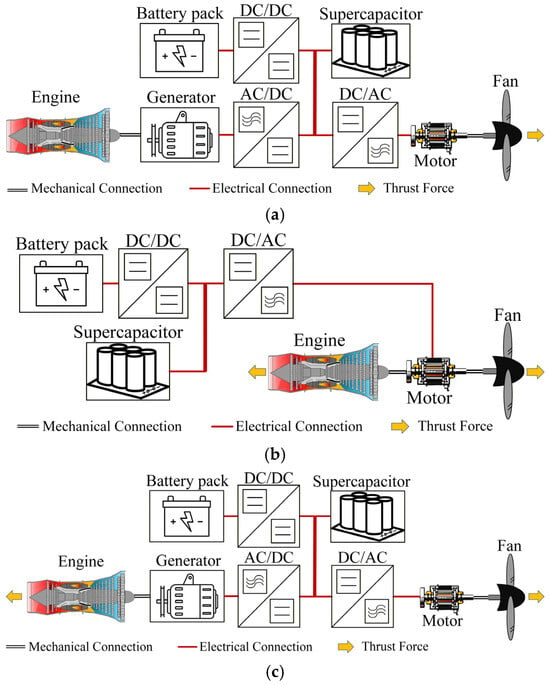
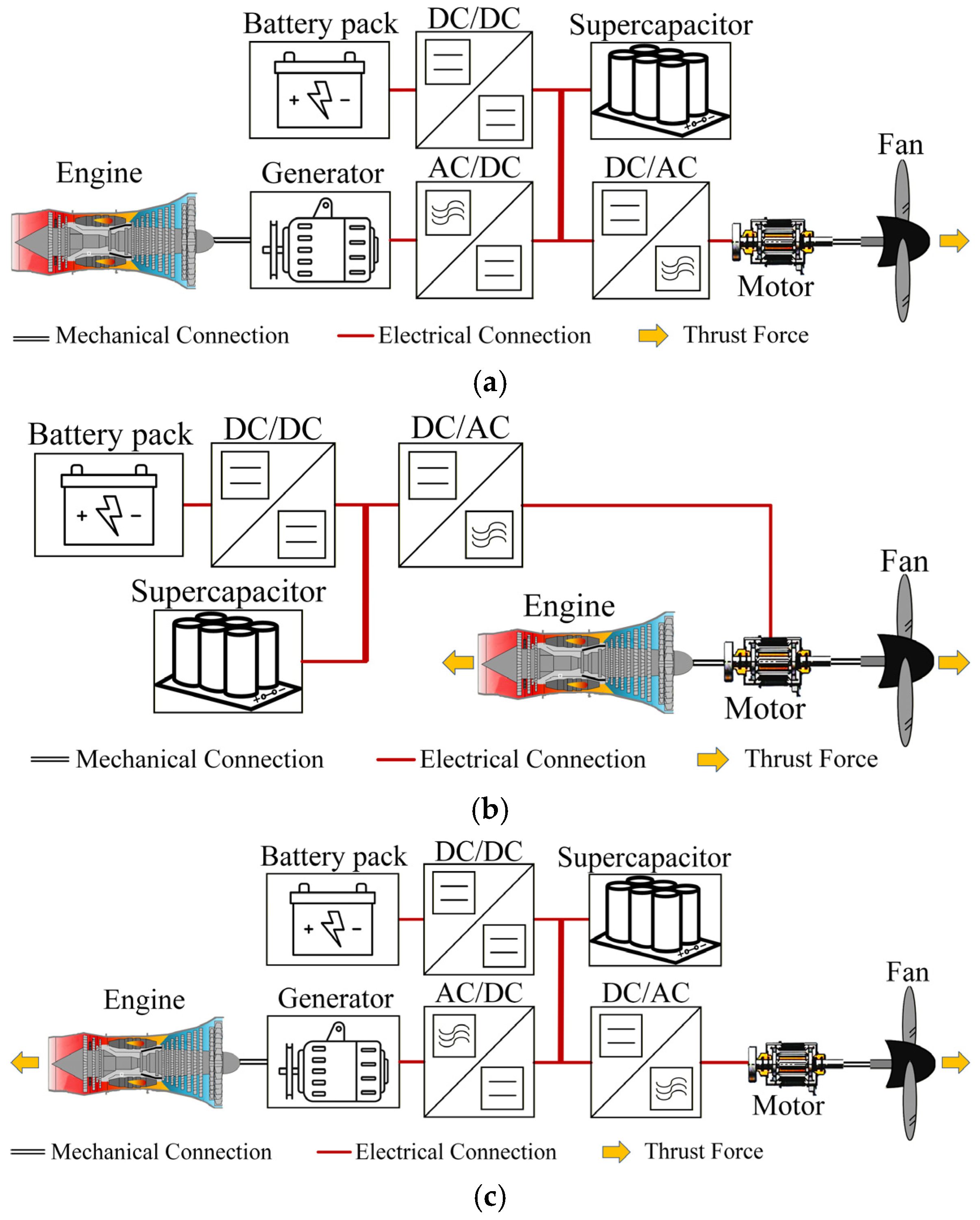
Hybrid electric aircraft (HEA) are increasingly being recognized as a viable and promising solution for the future of sustainable aviation [1,2]. HEA integrate traditional gas turbine engines with electrical components such as electric motors, batteries, and supercapacitors [3], thereby offering the potential to significantly enhance propulsion efficiency, reduce fuel consumption and emissions, and lay the foundation for the next generation of sustainable aviation [4]. The propulsion power system of HEA is categorized into three primary configurations, including series, parallel, and series-parallel types [5], as depicted in Figure 1. The key advantages and disadvantages of various propulsion power systems are summarized in Table 1. The electrical parts of the three architectures are structurally similar. Among them, the electrical structure of the series hybrid architecture is the most complex. Therefore, the series hybrid architecture is taken as an example for transient fault analysis. The transient fault analysis of other architectures can be inferred accordingly.

Figure 1. Configurations of HEA propulsion power systems. (a) Series hybrid power system, (b) Parallel hybrid power system, (c) Series-parallel hybrid power system.

Table 1. Advantages and disadvantages of propulsion power systems.

Architecture	Advantages	Disadvantages
Series	Optimal engine efficiency, simple electrical connection and highly flexible layout.	High weight of the equipment and lower power density.
Parallel	Lower energy loss and lighter device weight.	Complex mechanical coupling and suboptimal engine efficiency.
Series-parallel	Higher aerodynamic efficiency, lighter device weight and simpler mechanical structure.	Dependence on high-power electricity generation and transmission.

Compared with AC power systems, DC power systems have several unique advantages [6,7]: (1) DC systems do not have concepts such as frequency, phase, power angle stability, and reactive power, fundamentally avoiding the most complex stability and power factor issues in AC systems, resulting in more straightforward and direct control; (2) DC transmission is subject only to resistive losses, eliminating the additional energy dissipation caused by inductive and capacitive reactance prevalent in AC systems; (3) Through power electronic converters, the direction and magnitude of active power can be independently and precisely controlled at millisecond speeds. These characteristics collectively establish DC power systems as the preferred architecture for HEAs. Furthermore, HEAs equipped with DC power systems demonstrate superior compatibility with emerging high-power electrical loads and ultra-fast charging requirements, positioned as a forward-looking solution for future aviation electrification.

Despite its significant advantages, the DC system faces critical technical challenges. To meet the requirements for high capacity and power, DC power systems for HEA generally operate at a higher voltage and have a high degree of power electronics integration [8]. In the event of a short-circuit fault, such systems are not only exposed to significant safety risks but may also endanger personnel [9]. Therefore, fault protection has emerged as one of the most critical challenges requiring immediate attention in DC power systems.

Accurate transient modeling is fundamental for effective fault protection in DC power systems. Existing mature electromagnetic transient simulation platforms (such as PSCAD, MATLAB/Simulink, PLECS, etc.) are capable of accurately depicting the dynamic response characteristics of electrical systems, including the voltage, current, and power conversion processes at various nodes. However, the models constructed by these platforms essentially serve offline design verification, focusing on functional implementation and system-level performance evaluation. In contrast, what is urgently needed for the development of protection algorithms is a simplified transient model with clear structure, analyzable derivation, and physically meaningful parameters. Although such models make trade-offs in high-frequency details, they can accurately capture key characteristics of fault currents (such as rise rate, peak time, and steady-state trend) at extremely low computational cost, thus providing a solid mathematical foundation for real-time fault protection design.

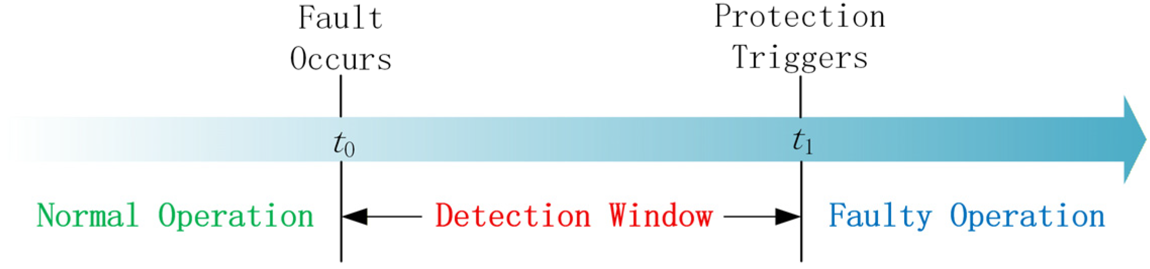
The transient model serves as a detection window before protective action, providing a decision-making basis for fault protection. Figure 2 illustrates the temporal relationship between the detection interval of transient modeling and the fault protection action. In this study, the scope of transient modeling research spans from the moment of fault occurrence t₀ to the moment of protection action triggering t₁. Fault protection typically include fault detection, fault isolation, and fault localization [10,11,12]. Fault identification involves determining system faults through the utilization of real-time monitoring data and advanced data analysis algorithms. The transient model serves as a benchmark for fault characteristics and plays a critical role in the design and validation of detection algorithms. Relevant methods include a feature vector learning-based method [13], a time-frequency analysis approach [14], dominant/lower order harmonic injection [15], and so on. Fault isolation entails rapidly disconnecting the faulty equipment or line via control switch devices (e.g., circuit breakers and disconnectors) to prevent fault propagation upon confirming the occurrence of a fault. The transient model provides a critical foundation for the selection of protection device parameters in fault isolation, such as a partitioning fault isolation strategy [16], an algorithm for relay tripping decision [17], and so on. Fault location identifies the precise position where the fault occurs. Transient models simulate faults at various locations to validate and calibrate fault location methods. Relevant methods include time-frequency reflectometry [18], RBF neural network with wavelet packet decomposition [19], deep learning-based algorithms [20], etc. In addition, the transient model also serves to suppress the initial surge current [21,22], which is the inevitable short-circuit current characterized by high amplitude and a rapid rate of rise, arising from the system inherent parameters. In conclusion, transient modeling of short-circuit faults in the HEA DC power system serves as a fundamental basis for effective fault identification, fault localization, and fault isolation.

Figure 2. The detection window of transient modeling.

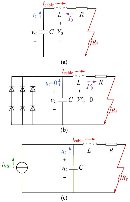
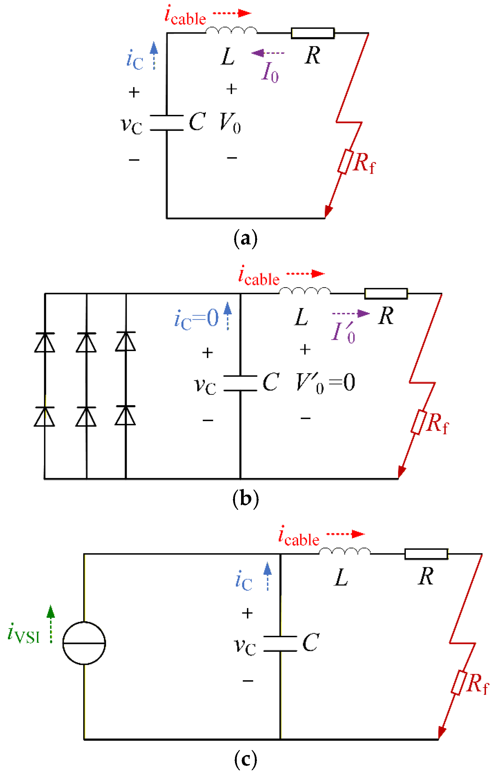
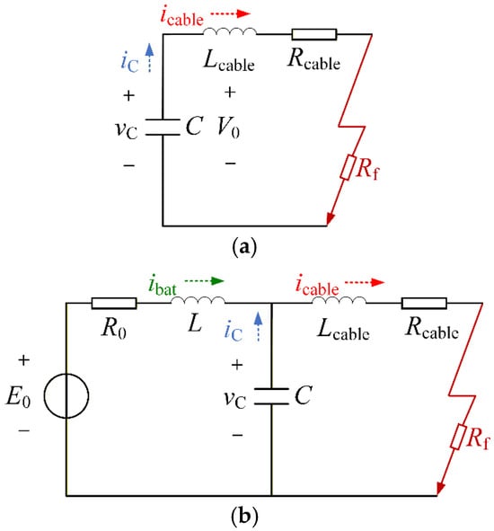
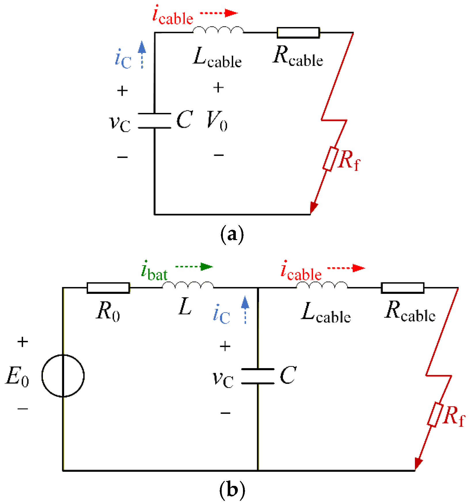
In the HEA DC power system, distributed components are broadly categorized into AC components and DC components. AC components, such as generators and fan motors, are connected to the DC bus through rectifiers or inverters. DC components, including power batteries and DC loads, interface with the DC bus via DC converters. When a short-circuit fault occurs on the DC bus, the transient fault current of the AC component includes three parts, the discharge current of the DC-link capacitor of the rectifier, the discharge current provided by the line through the freewheeling diode in the rectifier and the short-circuit current provided by the generator through the freewheeling diode in the rectifier [23,24], as illustrated in Figure 3. Meanwhile, the transient fault current of the DC component includes the discharge current of the DC-link capacitor of the converter and the short-circuit current during the free conduction stage of the diode [25,26], as shown in Figure 4. While previous studies have addressed transient modeling in HEA DC power systems, the dynamic control effects of power electronic converters are neglected, which reduces the accuracy of the fault transient model.

Figure 3. Previous modeling of AC components. (a) Capacitor discharge stage, (b) Simultaneous conduction stage of both diodes, (c) Natural commutation conduction stage of diodes.

Figure 4. Previous modeling of DC components. (a) Capacitor discharge stage, (b) Free conduction stage of diodes.

The interval between fault occurrence and detection is the most crucial stage in fault transient analysis. This time period typically ranges from several milliseconds to tens of milliseconds. Since the fault is not yet detected, the control system continues to operate under its normal control strategy. To achieve better performance in fault detection, isolation, and location, it is necessary to take into account the contribution of the converter control effect.

In this paper, considering the converter control effect, the transient modeling and analysis of the fault HEA DC power system are accomplished. The main contributions of this paper are as follows: (1) Transient modeling and analysis of individual distributed components, including generator and fan motor components, power battery components and DC load components; (2) Establishment of the transient model of the fault HEA DC power system.

The remaining part of this paper is organized as follows. Section 2 establishes the transient fault models of individual distributed components in the HEA DC power system and analyzes their transient fault characteristics. Section 3 develops a transient model of the fault HEA DC power system. The validity of the proposed model is validated through simulation experiments in Section 4. Section 5 presents the conclusions.

2. Transient Modeling of Individual Distributed Components

This section establishes transient models of short-circuit faults for each component in the HEA DC power system, including generator and fan motor components, power battery components, DC load components and supercapacitors. In addition, the transient fault characteristics of each component were analyzed.

2.1. Transient Model of Generator and Fan Motor Components

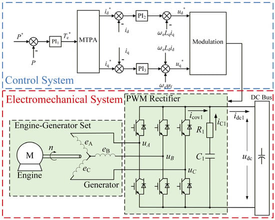
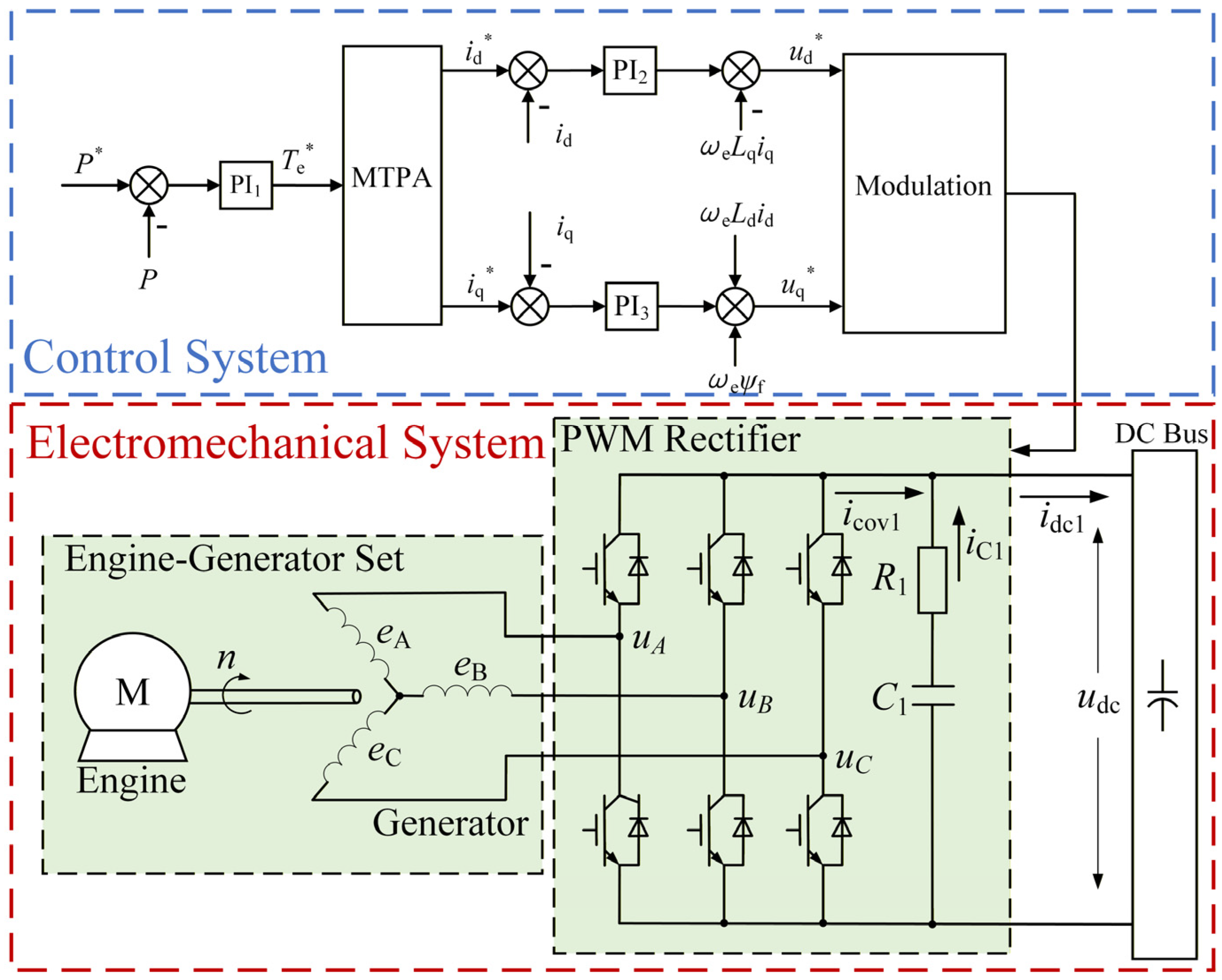
Generators and Fan Motors are the AC Components in the HEA DC power system. The PWM rectifier is used to connect the generator to the DC bus, while the inverter connects the fan motor to the bus. Due to their identical topology, a unified approach of modeling and analysis can be applied. The structure of the generator subsystem is illustrated in Figure 5.

Figure 5. The structure of the generator component.

To establish the mathematical model of the generator component, the system is divided into three relationships.

• The output–input relationship of the control system.

The double closed-loop PI control system is applied to the generator component, in which the inner loop is current control and the outer loop is power following control. The frequency domain expression of the PI controller can be expressed as:

$$H_{\alpha }(s)=K_{\mathrm{p}\alpha }+{\displaystyle \frac{K_{\mathrm{i}\alpha }}{s}},$$

(1)

where H_α respectively represent the inner and outer loop PI controllers of the d-axis and q-axis, K_pα is the proportionality coefficient of the PI controller, and K_iα is the integration coefficient of the PI controller.

The relationship between the relevant variables is

$$\left\{\begin{array}{l}{T}_{\mathrm{e}}^{*}=H_1(P^{*}-P)=(K_{\mathrm{p}1}+{\displaystyle \frac{K_{\mathrm{i}1}}{s}})(P^{*}-P)\\ i_{\mathrm{d}}^{*}=f_{\mathrm{d}}(T_{\mathrm{e}}^{*})\\ i_{\mathrm{q}}^{*}=f_{\mathrm{q}}(T_{\mathrm{e}}^{*})\\ u_{\mathrm{d}}^{*}=H_2(i_{\mathrm{d}}^{*}-i_{\mathrm{d}})-{\omega }_{\mathrm{e}}{L}_{\mathrm{q}}{i}_{\mathrm{q}}=(K_{\mathrm{p}2}+{\displaystyle \frac{K_{\mathrm{i}2}}{s}})(i_{\mathrm{d}}^{*}-i_{\mathrm{d}})-{\omega }_{\mathrm{e}}{L}_{\mathrm{q}}{i}_{\mathrm{q}}\\ u_{\mathrm{q}}^{*}=H_3(i_{\mathrm{q}}^{*}-i_{\mathrm{q}})+{\omega }_{\mathrm{e}}{L}_{\mathrm{d}}{i}_{\mathrm{d}}+{\omega }_{\mathrm{e}}{\psi }_{\mathrm{f}}=(K_{\mathrm{p}3}+{\displaystyle \frac{K_{\mathrm{i}3}}{s}})(i_{\mathrm{q}}^{*}-i_{\mathrm{q}})+{\omega }_{\mathrm{e}}{L}_{\mathrm{d}}{i}_{\mathrm{d}}+{\omega }_{\mathrm{e}}{\psi }_{\mathrm{f}}\end{array}\right.,$$

(2)

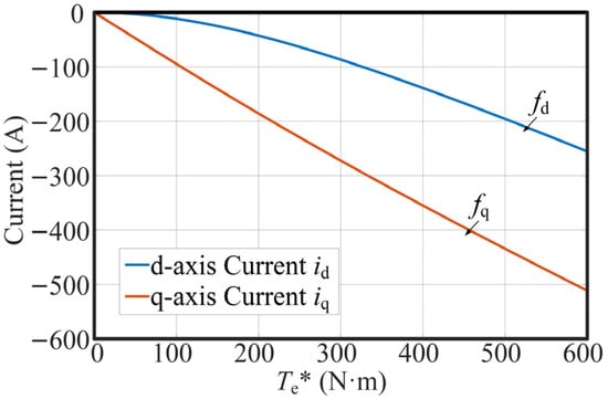
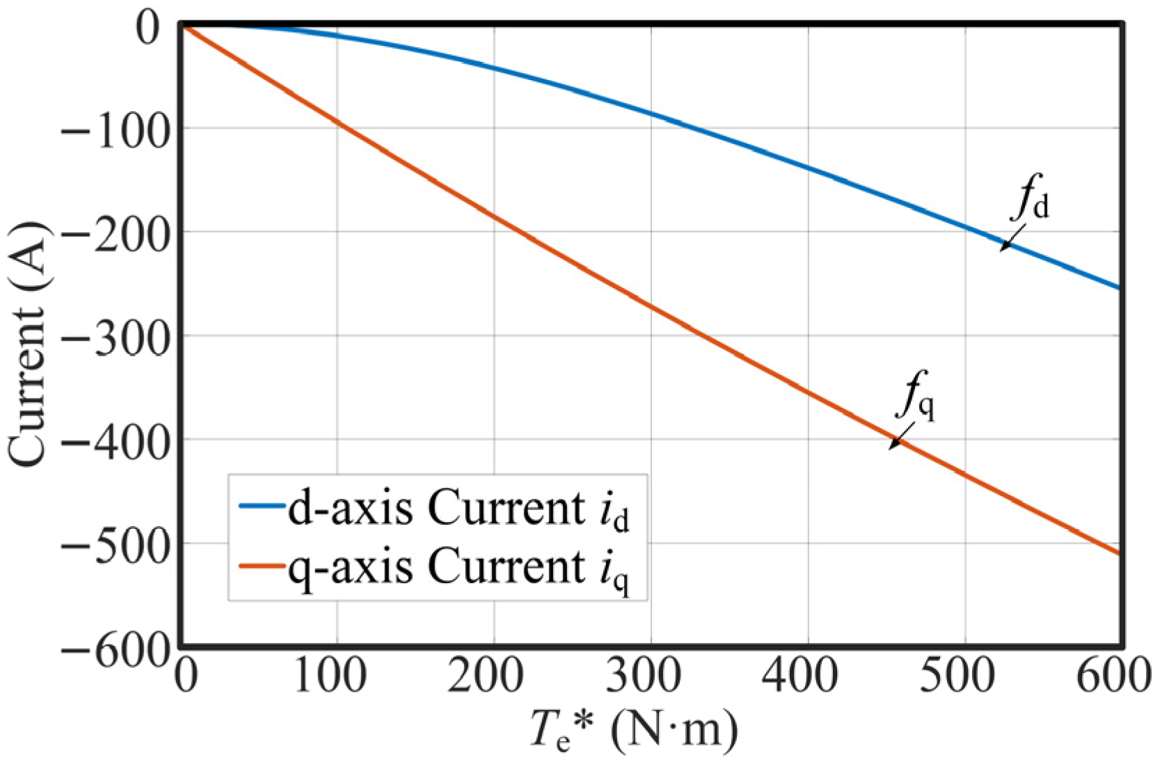
where the variables denoted with an asterisk, P*, T_e*, i_d*, i_q*, u_d*, and u_q*, represent the reference values of active power, electromagnetic torque, d-axis current, q-axis current, d-axis voltage, and q-axis voltage, respectively; whereas P, T_e, i_d, i_q, u_d, and u_q represent their corresponding measured values; f_d and f_q describe the relationship between the generator torque and current within the MTPA curve, which is based on the electromagnetic parameters of the PMSM and obtained through offline calibration and polynomial fitting, as shown in Figure 6; ω_e represents the electrical angular velocity of the motor; and ψ_f is the permanent magnet magnetic chain.

Figure 6. The relationship between the generator torque and d-axis and q-axis current.

Compared with the Euler transformation, the bilinear transformation has the advantages of rigorous stability preservation, capability to exactly match critical frequency responses, and superior numerical accuracy over a wide frequency range, which are essential for accurately capturing the dynamic behavior of the HEA DC power system. By the bilinear transformation method, Equation (2) is discretized to obtain

$$\left\{\begin{array}{ll}{T}_{\mathrm{e}}^{*}(k)& =T_{\mathrm{e}}^{*}(k-1)+(K_{\mathrm{p}1}+\frac{T}{2}{K}_{\mathrm{i}1})[P^{*}(k)-P(k)]-(K_{\mathrm{p}1}-\frac{T}{2}{K}_{\mathrm{i}1})[P^{*}(k-1)-P(k-1)]\hfill \\ i_{\mathrm{d}}^{*}(k)& =f_{\mathrm{d}}[T_{\mathrm{e}}^{*}(k)]\hfill \\ i_{\mathrm{q}}^{*}(k)& =f_{\mathrm{q}}[T_{\mathrm{e}}^{*}(k)]\hfill \\ u_{\mathrm{d}}^{*}(k)& =u_{\mathrm{d}}^{*}(k-1)+(K_{\mathrm{p}2}+\frac{T}{2}{K}_{\mathrm{i}2})[i_{\mathrm{d}}^{*}(k)-i_{\mathrm{d}}(k)]-(K_{\mathrm{p}2}-\frac{T}{2}{K}_{\mathrm{i}2})[i_{\mathrm{d}}^{*}(k-1)-i_{\mathrm{d}}(k-1)]\hfill \\ & -{\omega }_{\mathrm{e}}(k-1)L_{\mathrm{q}}{i}_{\mathrm{q}}(k-1)\hfill \\ u_{\mathrm{q}}^{*}(k)& =u_{\mathrm{q}}^{*}(k-1)+(K_{\mathrm{p}3}+\frac{T}{2}{K}_{\mathrm{i}3})[i_{\mathrm{q}}^{*}(k)-i_{\mathrm{q}}(k)]-(K_{\mathrm{p}2}-\frac{T}{2}{K}_{\mathrm{i}2})[i_{\mathrm{q}}^{*}(k)-i_{\mathrm{q}}(k)]\hfill \\ & +{\omega }_{\mathrm{e}}(k-1)L_{\mathrm{d}}{i}_{\mathrm{d}}(k-1)+{\omega }_{\mathrm{e}}(k-1){\psi }_{\mathrm{f}}\hfill \end{array},\right.$$

(3)

where T is sampling time interval.

2.

The output–input relationship of the modulation.

Since the maximum modulation voltage of the PWM rectifier is limited by the DC bus voltage, the PWM modulation may reach saturation when a short-circuit fault occurs. The relationship between its output and input can be expressed as follows.

(1) If $u_{\mathrm{dc}}\ge \sqrt{3({{u_{\mathrm{d}}}^{*}}^2+{{u_{\mathrm{q}}}^{*}}^2)},$

$$\left\{\begin{array}{l}{u}_{\mathrm{d}}={u_{\mathrm{d}}}^{*}\\ u_{\mathrm{q}}={u_{\mathrm{q}}}^{*}\end{array}\right..$$

(4)

(2) If $u_{\mathrm{dc}}<\sqrt{3({{u_{\mathrm{d}}}^{*}}^2+{{u_{\mathrm{q}}}^{*}}^2)},$

$$\left\{\begin{array}{l}{u}_{\mathrm{d}}={\displaystyle \frac{u_{\mathrm{dc}}}{\sqrt{3({{u_{\mathrm{d}}}^{*}}^2+{{u_{\mathrm{q}}}^{*}}^2)}}}{u_{\mathrm{d}}}^{*}\\ u_{\mathrm{q}}={\displaystyle \frac{u_{\mathrm{dc}}}{\sqrt{3({{u_{\mathrm{d}}}^{*}}^2+{{u_{\mathrm{q}}}^{*}}^2)}}}{u_{\mathrm{q}}}^{*}\end{array}\right..$$

(5)

3.

The relationship of the hardware circuit.

To focus on the electromagnetic-mechanical transient response analysis under fault conditions, it is assumed that the saturation and hysteresis losses of the motor core and the damping effects of the rotor can be ignored. The rationality of this simplification is based on the following considerations: (1) In typical medium and low-frequency operation scenarios, the amplitude of core loss is significantly lower than that of copper loss and mechanical power, having a negligible impact on the qualitative evolution trend of the main electromagnetic-mechanical transient process; (2) under the fundamental synchronous operation mode driven by rectifier/inverter, the direct influence of rotor eddy current effect on electromagnetic dynamics is relatively small, while the damping provided by the controller is much greater than the electromagnetic damping of the motor itself.

Under this simplification, the rotor air-gap magnetic field is modeled as a spatially sinusoidal distribution, resulting in balanced, purely sinusoidal back-electromotive forces in the stator three-phase windings. When the stator three-phase windings a, b, and c are converted to the two-phase rotating dq coordinate system, the voltage equation, flux linkage equation, and torque equation of the permanent magnet synchronous motor are respectively shown as follows.

$$\left[\begin{array}{c}{u}_{\mathrm{d}}\\ u_{\mathrm{q}}\end{array}\right]=\left[\begin{array}{cc}{R}_s& 0\\ 0& R_s\end{array}\right]\left[\begin{array}{c}{i}_{\mathrm{d}}\\ i_{\mathrm{q}}\end{array}\right]+{\displaystyle \frac{\mathrm{d}}{\mathrm{d}t}}\left[\begin{array}{c}{\psi }_{\mathrm{d}}\\ {\psi }_{\mathrm{q}}\end{array}\right]+\left[\begin{array}{cc}0& -{\omega }_{\mathrm{e}}\\ {\omega }_{\mathrm{e}}& 0\end{array}\right]\left[\begin{array}{c}{\psi }_{\mathrm{d}}\\ {\psi }_{\mathrm{q}}\end{array}\right],$$

(6)

$$\left[\begin{array}{c}{\psi }_{\mathrm{d}}\\ {\psi }_{\mathrm{q}}\end{array}\right]=\left[\begin{array}{cc}{L}_{\mathrm{d}}& 0\\ 0& L_{\mathrm{q}}\end{array}\right]\left[\begin{array}{c}{i}_{\mathrm{d}}\\ i_{\mathrm{q}}\end{array}\right]+\left[\begin{array}{c}{\psi }_{\mathrm{f}}\\ 0\end{array}\right],$$

(7)

$$T_{\mathrm{e}}={\displaystyle \frac{3}{2}}{p}_{\mathrm{n}}({\psi }_{\mathrm{d}}{i}_{\mathrm{q}}-{\psi }_{\mathrm{q}}{i}_{\mathrm{d}})={\displaystyle \frac{3}{2}}{p}_{\mathrm{n}}[{\psi }_{\mathrm{f}}{i}_{\mathrm{q}}+(L_{\mathrm{d}}-L_{\mathrm{q}})i_{\mathrm{d}}{i}_{\mathrm{q}}],$$

(8)

where u_d, u_q, i_d, i_q, ψ_d, ψ_q, L_d, L_q are respectively the d and q axis components of stator voltage, current, flux linkage, and inductance, R_s is the stator resistance, ω_e represents the electrical angular velocity of the motor, T_e is the electromagnetic torque, p_n is the number of PMSG pole-pairs, and ψ_f is the permanent magnet magnetic chain.

The dynamic equation of the motor’s rotation is

$$T_{\mathrm{m}}-T_{\mathrm{e}}=J{\displaystyle \frac{\mathrm{d}\omega }{\mathrm{d}t}},$$

(9)

where J is the moment of inertia of PMSG, ω is the mechanical angular velocity of the motor rotor, and T_m represents the output torque of the engine.

By using the equal-power coordinate transformation method, the switch function describing the PWM rectifier is transformed from the three-phase stationary abc coordinate system to the two-phase rotating dq coordinate system. Then, the switch function model of the PWM rectifier can be described as

$$\left\{\begin{array}{l}{u}_{\mathrm{d}}=u_{\mathrm{dc}}{s}_{\mathrm{d}}\\ u_{\mathrm{q}}=u_{\mathrm{dc}}{s}_{\mathrm{q}}\\ i_{\mathrm{cov}1}=i_{\mathrm{d}}{s}_{\mathrm{d}}+i_{\mathrm{q}}{s}_{\mathrm{q}}={\displaystyle \frac{u_{\mathrm{d}}{i}_{\mathrm{d}}+u_{\mathrm{q}}{i}_{\mathrm{q}}}{u_{\mathrm{dc}}}}\\ i_{\mathrm{dc}1}=i_{\mathrm{C}1}+i_{\mathrm{cov}1}\\ i_{\mathrm{C}1}=-C_1{\displaystyle \frac{\mathrm{d}{u}_{\mathrm{C}1}}{\mathrm{d}t}}\\ u_{\mathrm{C}1}=u_{\mathrm{dc}}-i_{\mathrm{C}1}{R}_1\\ P=u_{\mathrm{dc}}{i}_{\mathrm{dc}1}\end{array}\right.,$$

(10)

where s_d and s_q are the d and q axis components of the PWM rectifier switching function, which are determined by the control system output, u_dc is the DC Bus voltage, i_cov1 represents the output DC current by the generator after rectification, C₁ is the dc-link capacitor of the PWM rectifier, R₁ is the equivalent series resistance (ESR) of C₁, i_dc1 is the out current of the generator component, and P is the active power output by the generator component.

By the bilinear transformation method, Equations (6)–(10) is discretized to obtain

$$\left\{\begin{array}{l}{i}_{\mathrm{d}}(k+1)=i_{\mathrm{d}}(k)+\frac{T}{L_{\mathrm{d}}}[-R_{\mathrm{s}}{i}_{\mathrm{d}}(k)+{\omega }_{\mathrm{e}}(k)L_{\mathrm{q}}{i}_{\mathrm{q}}(k)+u_{\mathrm{d}}(k)]\\ i_{\mathrm{q}}(k+1)=i_{\mathrm{q}}(k)+\frac{T}{L_{\mathrm{q}}}[-R_{\mathrm{s}}{i}_{\mathrm{q}}(k)-{\omega }_{\mathrm{e}}(k)L_{\mathrm{d}}{i}_{\mathrm{d}}(k)-{\omega }_{\mathrm{e}}(k){\psi }_{\mathrm{f}}+u_{\mathrm{q}}(k)]\end{array}\right.,$$

(11)

$$T_{\mathrm{e}}(k)={\displaystyle \frac{3}{2}}{p}_{\mathrm{n}}[{\psi }_{\mathrm{f}}{i}_{\mathrm{q}}(k)+(L_{\mathrm{d}}-L_{\mathrm{q}})i_{\mathrm{d}}(k)i_{\mathrm{q}}(k)],$$

(12)

$$\omega (k+1)=\omega (k)+{\displaystyle \frac{T}{J}}[T_{\mathrm{m}}(k)-T_{\mathrm{e}}(k)],$$

(13)

$$\left\{\begin{array}{l}{i}_{\mathrm{cov}1}(k)=\frac{u_{\mathrm{d}}(k)i_{\mathrm{d}}(k)+u_{\mathrm{q}}(k)i_{\mathrm{q}}(k)}{u_{\mathrm{dc}}(k)}\\ i_{\mathrm{dc}1}(k)=-\frac{C_1}{T-R_1{C}_1}[u_{\mathrm{dc}}(k)-u_{\mathrm{dc}}(k-1)]-\frac{R_1{C}_1}{T-R_1{C}_1}[i_{\mathrm{cov}1}(k)-i_{\mathrm{cov}1}(k-1)+i_{\mathrm{dc}1}(k-1)]\\ P(k)=u_{\mathrm{dc}}(k)i_{\mathrm{dc}1}(k)\end{array}\right..$$

(14)

2.2. Transient Model of Faulty Power Battery Components

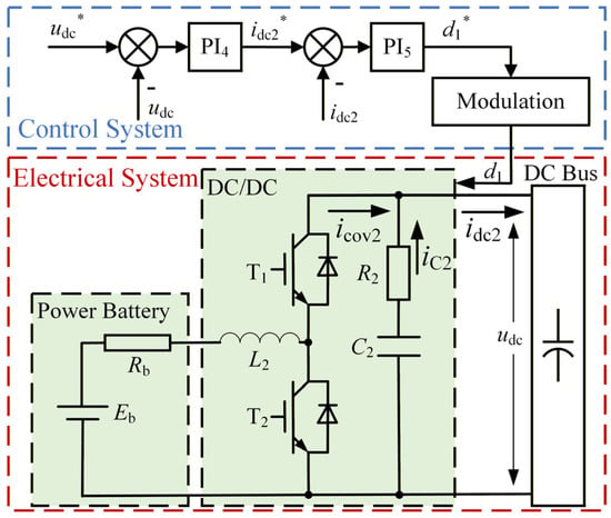
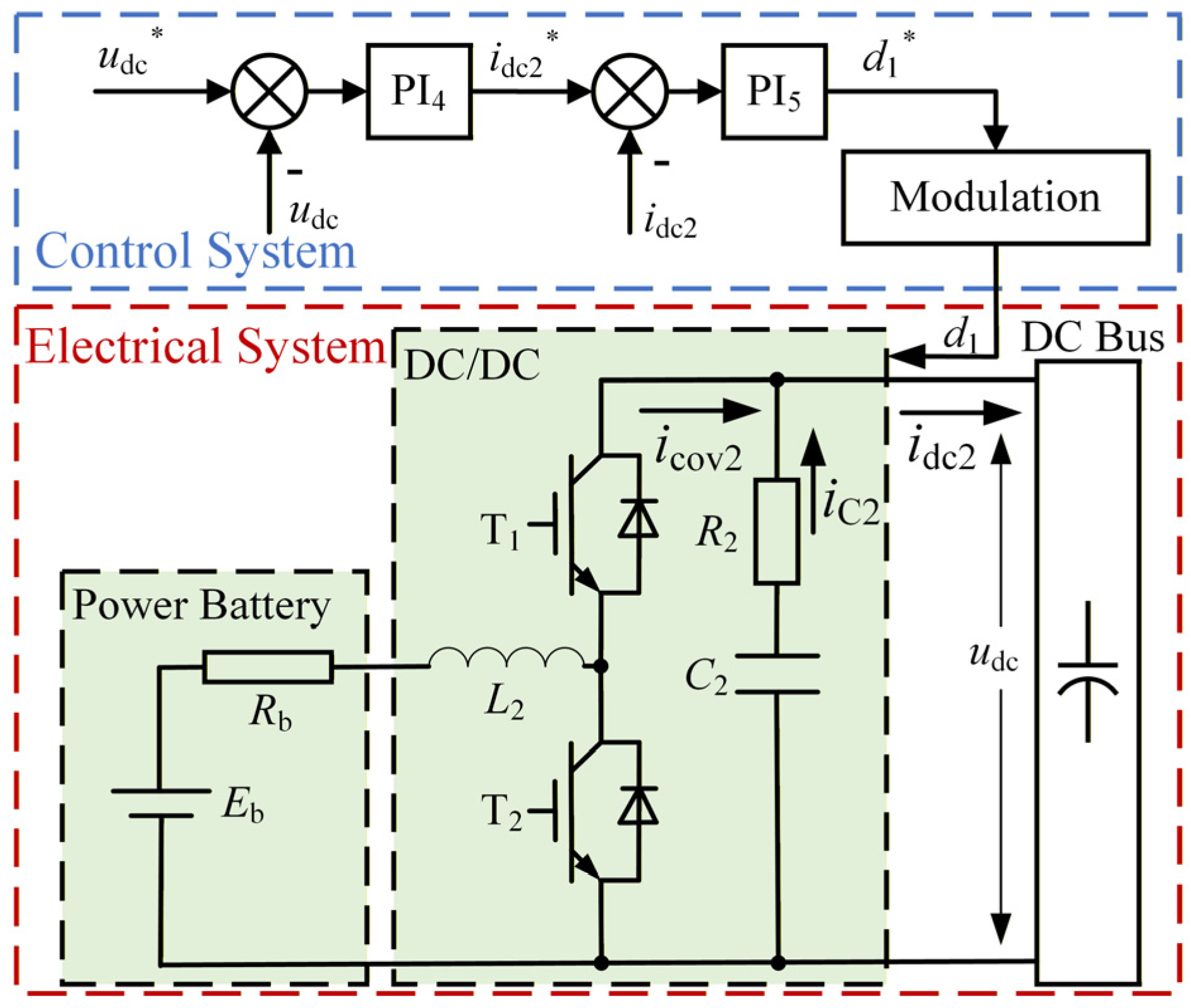
The power battery serves as a DC energy source for the HEA DC power system. The energy flow between the power battery and the DC bus is regulated by the bidirectional DC/DC converter, as shown in Figure 7. The transient modeling of the component is as follows and by the method described above.

Figure 7. The Structure of the power battery component.

• The output–input relationship of the control system.

The double closed-loop PI control system is applied to the power battery component, in which the inner loop is current control and the outer loop is voltage stability control. The relationship between the relevant variables is expressed as

$$\left\{\begin{array}{l}{i}_{\mathrm{dc}2}^{*}=H_4(u_{\mathrm{dc}}^{*}-u_{\mathrm{dc}})=(K_{\mathrm{p}4}+{\displaystyle \frac{K_{\mathrm{i}4}}{s}})(u_{\mathrm{dc}}^{*}-u_{\mathrm{dc}})\\ d_1^{*}=H_5(i_{\mathrm{dc}2}^{*}-i_{\mathrm{dc}2})=(K_{\mathrm{p}5}+{\displaystyle \frac{K_{\mathrm{i}5}}{s}})(i_{\mathrm{dc}2}^{*}-i_{\mathrm{dc}2})\end{array}\right.,$$

(15)

namely,

$$d_1^{*}=(K_{\mathrm{p}5}{K}_{\mathrm{p}4}+{\displaystyle \frac{K_{\mathrm{p}5}{K}_{\mathrm{i}4}+K_{\mathrm{p}4}{K}_{\mathrm{i}5}}{s}}+{\displaystyle \frac{K_{\mathrm{i}4}{K}_{\mathrm{i}5}}{s^2}})(u_{\mathrm{dc}}^{*}-u_{\mathrm{dc}})-(K_{\mathrm{p}5}+{\displaystyle \frac{K_{\mathrm{i}5}}{s}})i_{\mathrm{dc}2},$$

(16)

where u_dc* and i_dc2* denote the reference values of the bus voltage and the output current of the power battery subsystem, respectively, while u_dc and i_dc2 represent the corresponding measured values, and d₁* is the reference value of the T₁ duty cycle output by the control system.

By the bilinear transformation method, Equation (16) is discretized to obtain

$$\begin{array}{l}{d}_1^{*}(k)=2d_1^{*}(k-1)-d_1^{*}(k-2)\\ +[K_{\mathrm{p}5}{K}_{\mathrm{p}4}+\frac{1}{2}T(K_{\mathrm{p}5}{K}_{\mathrm{i}4}+K_{\mathrm{p}4}{K}_{\mathrm{i}5})+\frac{1}{4}{T}^2{K}_{\mathrm{i}4}{K}_{\mathrm{i}5}][u_{\mathrm{dc}}^{*}(k)-u_{\mathrm{dc}}(k)]\\ +[\frac{1}{2}{T}^2{K}_{\mathrm{i}4}{K}_{\mathrm{i}5}-2K_{\mathrm{p}5}{K}_{\mathrm{p}4}][u_{\mathrm{dc}}^{*}(k-1)-u_{\mathrm{dc}}(k-1)]\\ +[K_{\mathrm{p}5}{K}_{\mathrm{p}4}-\frac{1}{2}T(K_{\mathrm{p}5}{K}_{\mathrm{i}4}+K_{\mathrm{p}4}{K}_{\mathrm{i}5})+\frac{1}{4}{T}^2{K}_{\mathrm{i}4}{K}_{\mathrm{i}5}][u_{\mathrm{dc}}^{*}(k-2)-u_{\mathrm{dc}}(k-2)]\\ -(K_{\mathrm{p}5}+\frac{1}{2}T{K}_{\mathrm{i}5})i_{\mathrm{dc}2}(k)+2K_{\mathrm{p}5}{i}_{\mathrm{dc}2}(k-1)-(K_{\mathrm{p}5}-\frac{1}{2}T{K}_{\mathrm{i}5})i_{\mathrm{dc}2}(k-2)\end{array}.$$

(17)

2.

The output–input relationship of the modulation.

When the bus voltage is higher than the output voltage of the power battery, the converter is in boost mode. When the bus voltage is lower than the battery voltage, the reverse diode of T₁ becomes conductive, and the converter operates in the direct-through mode. Mathematically, it can be equivalent to d₁ = 1 in the above-mentioned boost mode, and its derivation process will not be elaborated here. The relationship between its output and input can be expressed as follows.

$$\left\{\begin{array}{cc}{d}_1=d_1^{*}& ,u_{\mathrm{dc}}>E_{\mathrm{b}}\\ d_1=1& ,u_{\mathrm{dc}}\le E_{\mathrm{b}}\end{array}\right.,$$

(18)

where d₁ represents the actual value of the T₁ duty cycle output by the control system.

3.

The relationship of the hardware circuit.

According to the state space averaging method, the state average model of the system is obtained.

$$\left\{\begin{array}{cc}\hfill L_2{\displaystyle \frac{\mathrm{d}}{\mathrm{d}t}}{i}_{\mathrm{cov}2}& =-(R_{\mathrm{b}}+R_{\mathrm{L}2})i_{\mathrm{cov}2}+E_{\mathrm{b}}-d_1{u}_{\mathrm{dc}}\hfill \\ \hfill i_{\mathrm{dc}2}& =i_{\mathrm{C}2}+i_{\mathrm{cov}2}\hfill \\ \hfill i_{\mathrm{C}2}& =-C_2{\displaystyle \frac{\mathrm{d}{u}_{\mathrm{C}2}}{\mathrm{d}t}}\hfill \\ \hfill u_{\mathrm{C}2}& =u_{\mathrm{dc}}-i_{\mathrm{C}2}{R}_2\hfill \end{array}\right.,$$

(19)

where L₂ is the inductance of the converter, R_L2 is the resistance of the inductance coil, E_b is the electromotive force of the battery, R_b is the internal resistance of the battery, C₂ is the dc-link capacitor of the converter, R₂ is the equivalent series resistance (ESR) of C₂, i_cov2 is the current output by the battery after passing through the converter, and i_dc2 is the output current of the power battery component.

By the backward difference method, Equation (19) is discretized to obtain

$$\left\{\begin{array}{l}{i}_{\mathrm{cov}2}(k)=\frac{L_2}{L_2+T(R_{\mathrm{b}}+R_{\mathrm{L}2})}{i}_{\mathrm{cov}2}(k-1)+\frac{T{E}_{\mathrm{b}}}{L_2+T(R_{\mathrm{b}}+R_{\mathrm{L}2})}-\frac{T{d}_1(k)u_{\mathrm{dc}}(k)}{L_2+T(R_{\mathrm{b}}+R_{\mathrm{L}2})}\\ i_{\mathrm{dc}2}(k)=-\frac{C_2}{T-R_2{C}_2}[u_{\mathrm{dc}}(k)-u_{\mathrm{dc}}(k-1)]-\frac{R_2{C}_2}{T-R_2{C}_2}[i_{\mathrm{dc}2}(k-1)-i_{\mathrm{cov}2}(k-1)]+i_{\mathrm{cov}2}(k)\end{array}\right..$$

(20)

2.3. Transient Model of DC Load Components

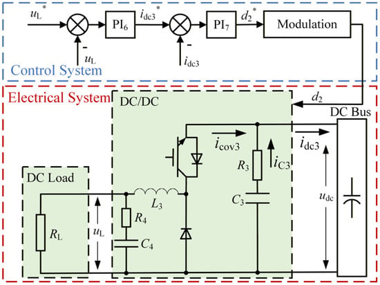
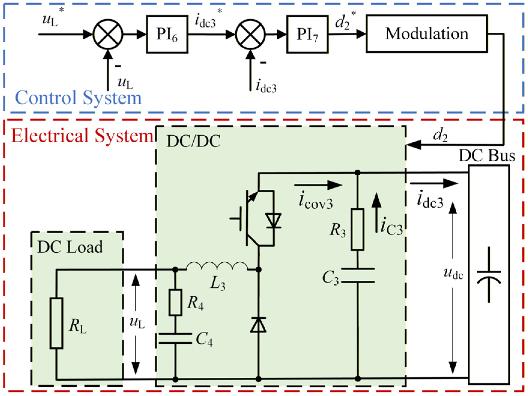
The structure of the DC load components is shown in Figure 8. The transient modeling of the components is as follows by the method described above.

Figure 8. The structure of the DC load components.

• The output–input relationship of the control system

The relationship between the relevant variables in the control system of the DC load is expressed as

$$\left\{\begin{array}{l}{i}_{\mathrm{dc}3}^{*}=H_6(u_{\mathrm{L}}^{*}-u_{\mathrm{L}})=(K_{\mathrm{p}6}+{\displaystyle \frac{K_{\mathrm{i}6}}{s}})(u_{\mathrm{L}}^{*}-u_{\mathrm{L}})\\ d_2^{*}=H_7(i_{\mathrm{dc}3}^{*}-i_{\mathrm{dc}3})=(K_{\mathrm{p}7}+{\displaystyle \frac{K_{\mathrm{i}7}}{s}})(i_{\mathrm{dc}3}^{*}-i_{\mathrm{dc}3})\end{array}\right.,$$

(21)

that is,

$$d_2^{*}=(K_{\mathrm{p}7}{K}_{\mathrm{p}6}+{\displaystyle \frac{K_{\mathrm{p}7}{K}_{\mathrm{i}6}+K_{\mathrm{p}6}{K}_{\mathrm{i}7}}{s}}+{\displaystyle \frac{K_{\mathrm{i}6}{K}_{\mathrm{i}7}}{s^2}})(u_{\mathrm{L}}^{*}-u_{\mathrm{L}})-(K_{\mathrm{p}7}+{\displaystyle \frac{K_{\mathrm{i}7}}{s}})i_{\mathrm{dc}3},$$

(22)

where u_L* and i_dc3* denote the reference values of the bus voltage and the output current of the power battery subsystem, respectively, while u_L and i_dc3 represent the corresponding measured values, and d₂* is the reference value of the T₁ duty cycle output by the control system.

By the bilinear transformation method, Equation (22) is discretized to obtain

$$\begin{array}{ll}\hfill d_2^{*}(k)& =2d_2^{*}(k-1)-d_2^{*}(k-2)\\ & +[K_{\mathrm{p}7}{K}_{\mathrm{p}6}+\frac{1}{2}T(K_{\mathrm{p}7}{K}_{\mathrm{i}6}+K_{\mathrm{p}6}{K}_{\mathrm{i}7})+\frac{1}{4}{T}^2{K}_{\mathrm{i}6}{K}_{\mathrm{i}7}][u_{\mathrm{L}}^{*}(k)-u_{\mathrm{L}}(k)]\\ & +[\frac{1}{2}{T}^2{K}_{\mathrm{i}6}{K}_{\mathrm{i}7}-2K_{\mathrm{p}7}{K}_{\mathrm{p}6}][u_{\mathrm{L}}^{*}(k-1)-u_{\mathrm{L}}(k-1)]\\ & +[K_{\mathrm{p}7}{K}_{\mathrm{p}6}-\frac{1}{2}T(K_{\mathrm{p}7}{K}_{\mathrm{i}6}+K_{\mathrm{p}6}{K}_{\mathrm{i}7})+\frac{1}{4}{T}^2{K}_{\mathrm{i}6}{K}_{\mathrm{i}7}][u_{\mathrm{L}}^{*}(k-2)-u_{\mathrm{L}}(k-2)]\\ & -(K_{\mathrm{p}7}+\frac{1}{2}T{K}_{\mathrm{i}7})i_{\mathrm{dc}3}(k)+2K_{\mathrm{p}7}{i}_{\mathrm{dc}3}(k-1)-(K_{\mathrm{p}7}-\frac{1}{2}T{K}_{\mathrm{i}7})i_{\mathrm{dc}3}(k-2)\end{array}$$

(23)

2.

The output–input relationship of the modulation.

The output–input relationship of the modulation is expressed as

$$d_2=d_2^{*}$$

(24)

where d₂ represents the actual value of the duty cycle output by the control system.

3.

The relationship of the hardware circuit.

According to the state space averaging method, the state average model of the system is obtained in Equation (25).

$$\left\{\begin{array}{l}{C}_{\mathrm{L}}{\displaystyle \frac{\mathrm{d}}{\mathrm{d}t}}{u}_{\mathrm{L}}=-{\displaystyle \frac{u_{\mathrm{L}}}{R_{\mathrm{L}}}}-i_{\mathrm{cov}3}\\ L_3{\displaystyle \frac{\mathrm{d}}{\mathrm{d}t}}{i}_{\mathrm{cov}3}=-R_{\mathrm{L}3}{i}_{\mathrm{cov}3}-u_{\mathrm{L}}+d_2{u}_{\mathrm{dc}}\\ i_{\mathrm{dc}3}=i_{\mathrm{C}3}+i_{\mathrm{cov}3}\\ i_{\mathrm{C}3}=-C_3{\displaystyle \frac{\mathrm{d}{u}_{\mathrm{C}3}}{\mathrm{d}t}}\\ u_{\mathrm{C}3}=u_{\mathrm{dc}}-i_{\mathrm{C}3}{R}_3\end{array}\right.,$$

(25)

where L₃ is the inductance of the converter, R_L3 is the resistance of the inductance coil, u_L is the load voltage, R_L is the resistance of the DC load, C₃ is the dc-link capacitor of the converter, R₃ is the equivalent series resistance (ESR) of C₃, C_L is the dc-link capacitor of the DC load, i_cov3 is the current output of the converter, and i_dc3 is the output current of the DC load component.

By the backward difference method, Equation (25) is discretized to obtain

$$\left\{\begin{array}{l}{u}_{\mathrm{L}}(k)=\frac{R_{\mathrm{L}}{C}_{\mathrm{L}}}{R_{\mathrm{L}}{C}_{\mathrm{L}}+T}{u}_{\mathrm{L}}(k-1)-\frac{T{R}_{\mathrm{L}}}{T+R_{\mathrm{L}}{C}_{\mathrm{L}}}{i}_{\mathrm{cov}3}(k-1)\\ i_{\mathrm{cov}3}(k)=\frac{L_3}{L_3+T{R}_{\mathrm{L}3}}{i}_{\mathrm{cov}3}(k-1)-\frac{T}{L_3+T{R}_{\mathrm{L}3}}{u}_{\mathrm{L}}(k)+\frac{T{d}_2(k)}{L_3+T{R}_{\mathrm{L}3}}{u}_{\mathrm{dc}}(k)\\ i_{\mathrm{dc}3}(k)=-\frac{C_3}{T-R_3{C}_3}[u_{\mathrm{dc}}(k)-u_{\mathrm{dc}}(k-1)]-\frac{R_3{C}_3}{T-R_3{C}_3}[i_{\mathrm{dc}3}(k-1)-i_{\mathrm{cov}3}(k-1)]+i_{\mathrm{cov}3}(k)\end{array}\right.$$

(26)

2.4. Transient Model of Supercapacitor

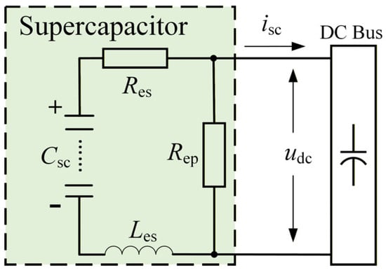
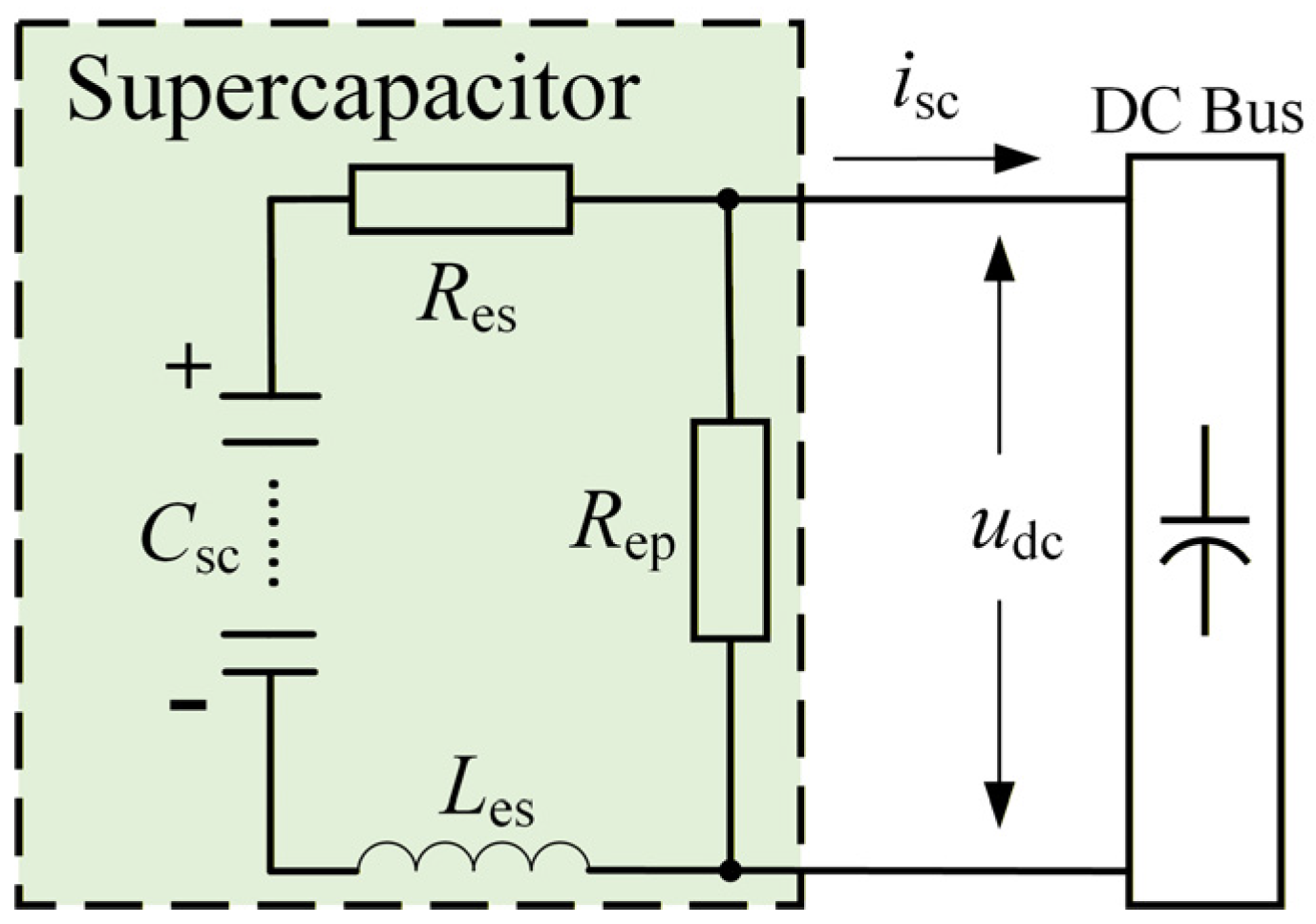
The supercapacitor is directly connected to the DC bus and function as a filter to mitigate the fluctuations of the bus voltage. Its equivalent model is shown in Figure 9, where C_sc represents the ideal capacitance, R_es denotes the equivalent series resistance (ESR) of the supercapacitor, L_es denotes the equivalent series inductance (ESL) of the supercapacitor, R_ep is the equivalent self-discharge resistance of the supercapacitor, and i_sc is the output current of the supercapacitor. Ignoring the current flowing through R_ep, the output current of the supercapacitor can be obtained by Equation (27).

$$\left\{\begin{array}{l}{i}_{\mathrm{sc}}=-C_{\mathrm{sc}}{\displaystyle \frac{\mathrm{d}{u}_{\mathrm{sc}}}{\mathrm{d}t}}\\ u_{\mathrm{sc}}=u_{\mathrm{dc}}+i_{\mathrm{sc}}{R}_{\mathrm{es}}+L_{\mathrm{es}}{\displaystyle \frac{\mathrm{d}{i}_{\mathrm{sc}}}{\mathrm{d}t}}\end{array}\right..$$

(27)

Figure 9. The equivalent model of the supercapacitor.

By the backward difference method, Equation (27) is discretized to obtain

$$i_{\mathrm{sc}}(k)=\frac{2C_{\mathrm{sc}}+T{R}_{\mathrm{es}}{C}_{\mathrm{sc}}}{C_{\mathrm{sc}}+T{R}_{\mathrm{es}}{C}_{\mathrm{sc}}-T^2}{i}_{\mathrm{sc}}(k-1)-\frac{C_{\mathrm{sc}}}{C_{\mathrm{sc}}+T{R}_{\mathrm{es}}{C}_{\mathrm{sc}}-T^2}{i}_{\mathrm{sc}}(k-2)-T[u_{\mathrm{dc}}(k)-u_{\mathrm{dc}}(k-1)].$$

(28)

3. Transient Modeling of Faulty HEA DC Power System

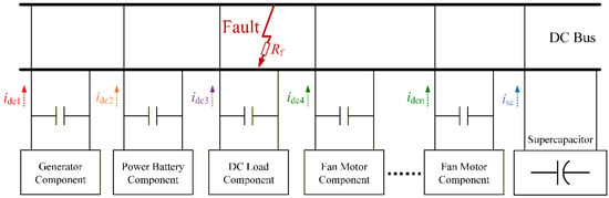
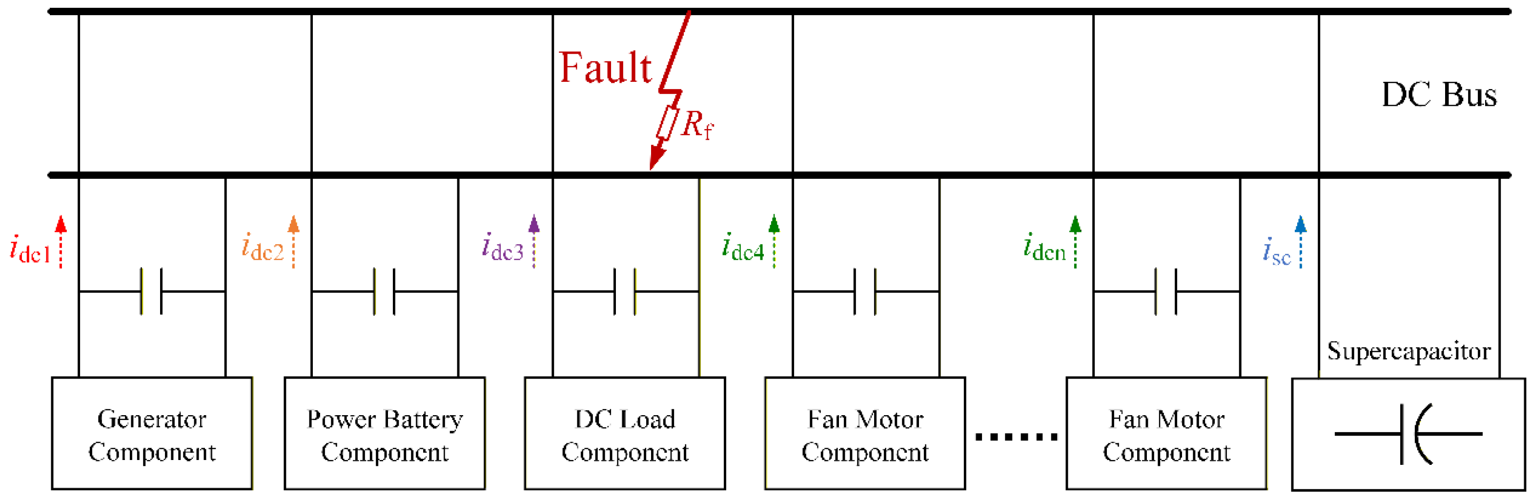
This section combines the transient models of individual distributed components to establish a comprehensive transient model for the faulty HEA DC power system. In this paper, bus short-circuit faults are adopted as the representative fault type for analysis. Short-circuit faults in the busbar cable, branch cables, and internal switching devices of converters are all equivalently modeled as bus short-circuit faults. Busbar short-circuit faults are adopted as the representative fault type for analysis, as illustrated in Figure 10.

Figure 10. The transient model of the faulty HEA DC power system.

The bus voltage and the output currents of individual components are critical state variables for characterizing the transient behavior of the faulty HEA DC power system. The relationship between the bus voltage and the output current of each converter is

$$i_{\mathrm{sc}}={\displaystyle \sum _{\mathrm{j}=1}^{\mathrm{n}}{i}_{\mathrm{dcj}}}-{\displaystyle \frac{u_{\mathrm{dc}}}{R_{\mathrm{f}}}},$$

(29)

where R_f denotes the short-circuit fault resistance, i_f represents the fault current, and i_dcj denotes the output current of converter j (j = 1, …, n).

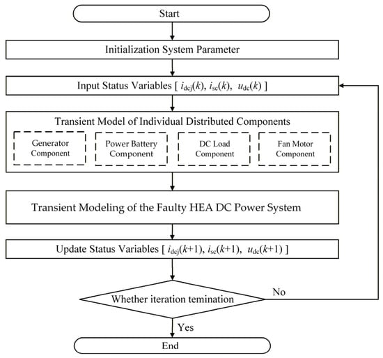
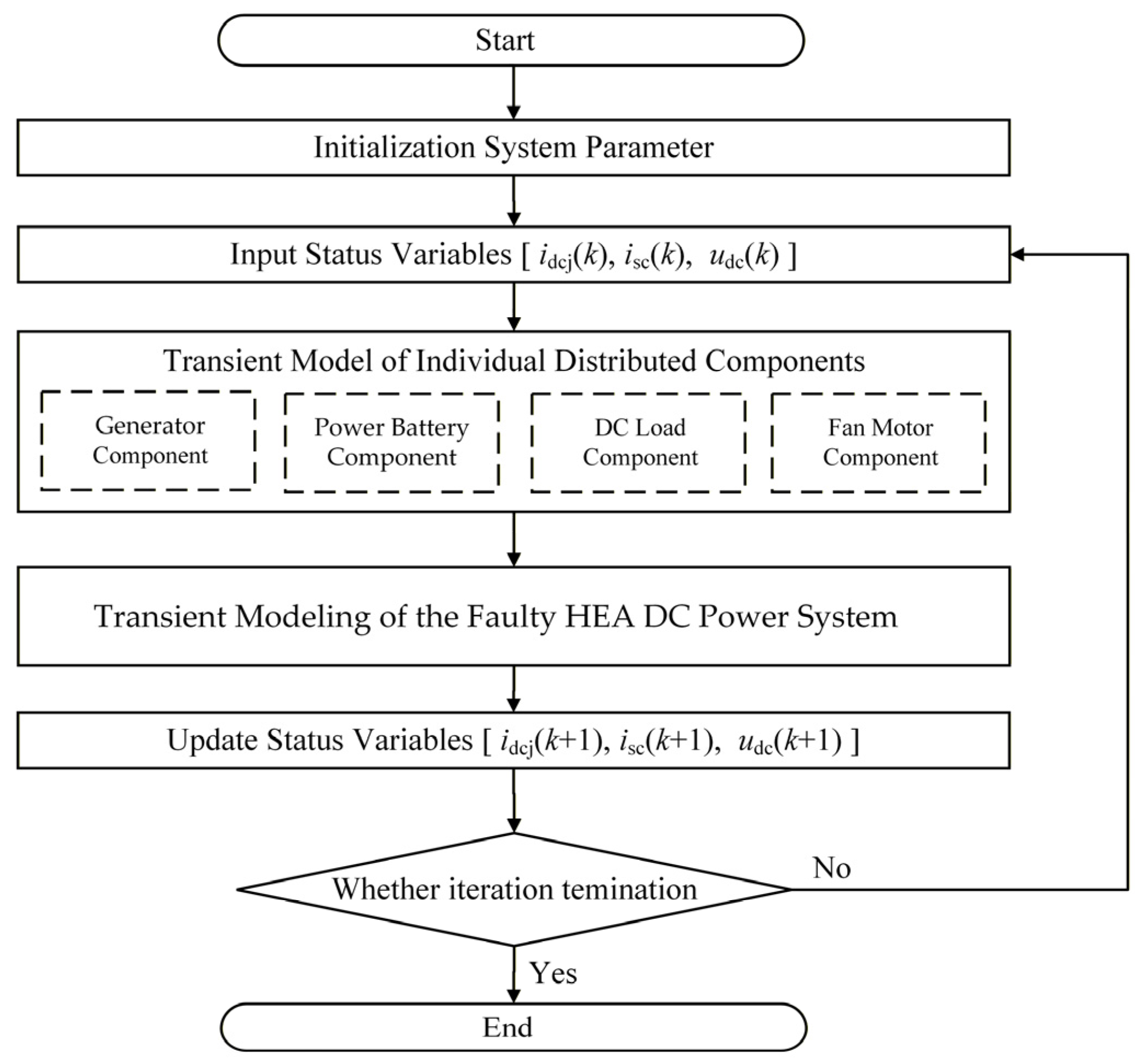
Based on the aforementioned model, the transient fault analysis procedure for the HEA DC power system is summarized as follows.

Step 1: Initialize all parameters, including the system parameters of each distributed component and the initial values of bus voltage and each output current. Meanwhile, a short-circuit fault condition is set.

Step 2: According to the transient models of independent distributed components, the output current of each component is computed, including generator and fan motor components, battery component and DC load component.

Step 3: Based on the transient fault model of the HEA DC power system, the output currents are substituted by these obtained in Step 2 to update the bus voltage. Simultaneously the output current of the supercapacitor is solved.

Step 4: Iterate Steps 2 and 3 until the iteration end condition is reached.

The overall process of transient fault analysis for the HEA DC power system is shown in Figure 11.

Figure 11. The process of transient fault analysis for the HEA DC power system.

4. Simulation Experiments and Analysis

To validate the proposed model, the transient models were utilized in numerical simulations and compared with the semi-physical simulation test platform and the previous method. Subsequently, the experimental results were analyzed to draw conclusions.

4.1. Semi-Physical Test System

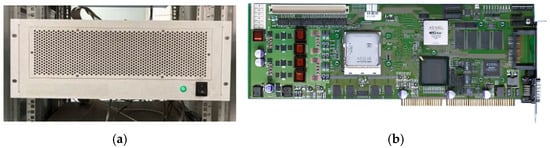
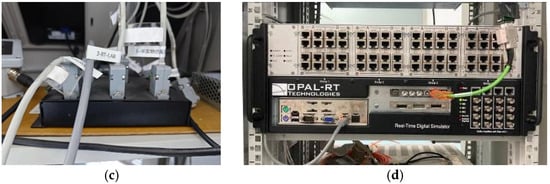
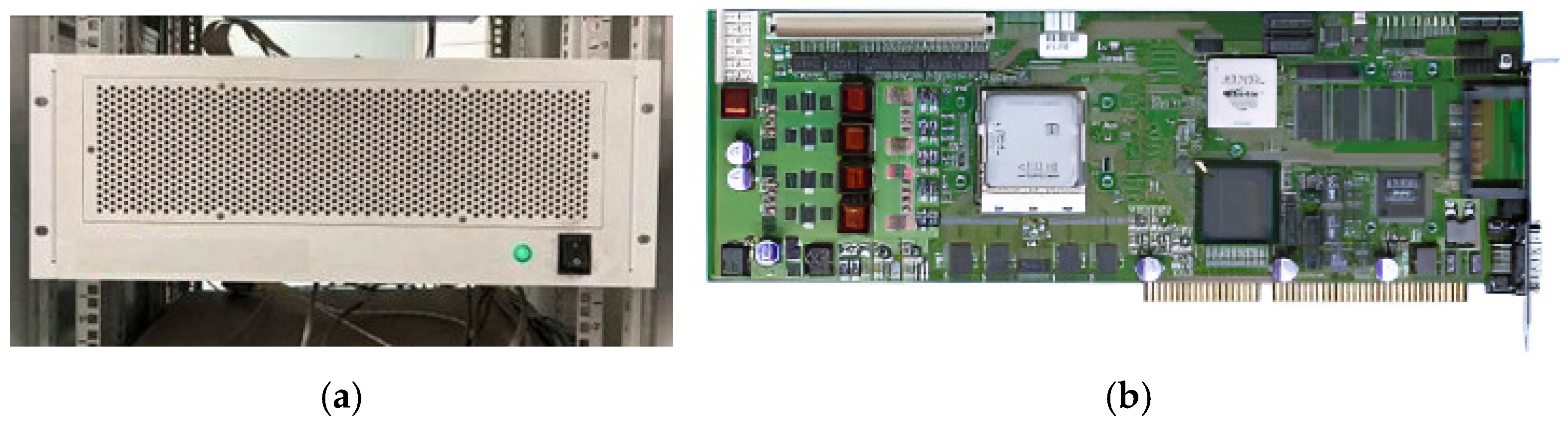
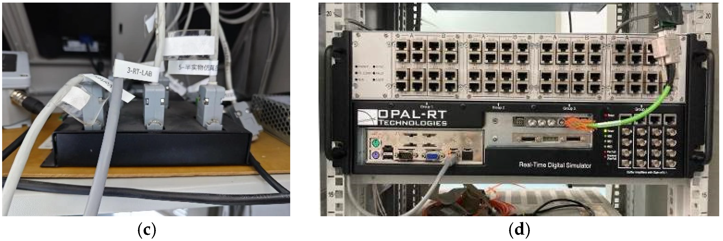
Semi-physical simulation, also known as hardware-in-the-loop simulation, is an important means for system development and principle verification. The semi-physical simulation test platform is composed of the rapid control prototype system and the RT-Lab simulator, as shown in Figure 12. The rapid control prototype system connects the DS1006 processor board card and the Flex Ray bus communication relay to output control signals externally and receive feedback signals from the controlled object. The controlled object is simulated and realized by the RT-Lab simulator.

Figure 12. The HEA DC power system semi-physical simulation test platform. (a) Rapid control prototype system, (b) DS1006 processor board card, (c) Flex Ray bus communication, (d) RT-Lab simulator.

Taking the series hybrid power system shown in Figure 1a as an example, the HEA DC power system was constructed on the semi-physical simulation test platform. The parameters of the generator, motor, circuit and load used in the semi-physical simulation test platform are all derived from the real component data sheets provided by the partners and the previous test results of the subsystems. Therefore, the dynamic characteristics of the system can be accurately reproduced.

Although the semi-physical simulation test platform significantly enhances the practical relevance of the study, it is necessary to acknowledge the inherent limitations of this simulation approach in replicating physical reality. Firstly, constrained by the selected simulation step size and discrete solver, the model cannot accurately reproduce electromagnetic transients with frequencies higher than the theoretical Nyquist limit, and their responses will be smoothed or aliased. Secondly, the input/output and communication delays in the signal chain introduce additional phase lag, which may slightly affect the stability margin of the closed-loop system when the controller bandwidth is high. Thirdly, although the parameters of the numerical model are set based on the nominal values of the target motor, the hysteresis, saturation, and temperature rise effects in the actual physical system are difficult to fully match, which may lead to response deviations under extreme operating conditions. Therefore, these factors limit the fidelity of the semi-physical system in reproducing extremely rapid transient phenomena, and the experimental results should mainly be regarded as verification of the dominant dynamic characteristics rather than an absolute reproduction of the physical prototype at the quantitative level.

A DC inter-pole short-circuit fault was configured on the semi-physical simulation test platform for the HEA DC power system. The short-circuit fault resistance was set to 1 Ω, 0.1 Ω, and 0.01 Ω, respectively, to simulate varying levels of fault severity. These resistance values serve as representative cases in the analysis, and alternative values may be employed depending on specific application requirements. The simulation duration is set to 100 ms, which considers that the model is specifically designed for fault detection and early-stage diagnosis, capturing the transient system dynamics immediately following fault inception is critical. Extending the simulation duration would be appropriate for analyses targeting longer-term behavioral evolution. The sampling time is set based on the empirical rule that the sampling frequency should be at least 10 to 30 times the system bandwidth. In the HEA power system, the controlled object is various converters, and their closed-loop control bandwidth is approximately 8~16 kHz. To ensure sufficient time-domain response fidelity and avoid aliasing, the sampling frequency is chosen as

$$f_s=30\times 16 \mathrm{kHz}\approx 500 \mathrm{kHz},$$

(30)

which corresponds to a sampling time of

$$h=1/f_s=2 \mathsf{\mu }\mathrm{s}.$$

(31)

Meanwhile, as the primary control unit, the TMS320F28335 digital signal processor (Texas Instruments, Dallas, TX, USA) features a maximum system clock frequency of 150 MHz. The sampling interval is sufficient to accommodate one complete execution cycle of the control algorithm, including ADC sampling, state estimation, feedback control computation, and PWM output update. Table 2 summarizes the key parameters of the system, including the hardware system and the control system. Subsequently, the results were analyzed in detail.

Table 2. System parameters.

Hardware System				Control System
Parameters	Value	Parameters	Value	Parameters	Value
Rs	7.5 mΩ	L3	5 mH	Kp1	600
Ld	0.8 mH	RL3	3 mΩ	Ki1	60
Lq	0.8 mH	C3	1000 μF	Kp2	0.5
Ψf	0.538 Wb	R3	10 mΩ	Ki2	10
pn	4	C4	1000 μF	Kp3	1
J	0.3085 kg·m2	R4	10 mΩ	Ki3	10
Tm	630 N·m	RL	10 Ω	Kp4	0.1
C1	24,000 μF	Csc	2.5 F	Ki4	2
R1	0.5 Ω	Res	62.1 mΩ	Kp5	8
Eb	650 V	Les	100 nH	Ki5	1.5
Rb	230 mΩ	Rep	100 kΩ	Kp6	1
L2	16.7 mH			Ki6	10
RL2	1 mΩ			Kp7	0.015
C2	1000 μF			Ki7	10
R2	10 mΩ			T	2 × 10−6 s

4.2. Verification of Transient Modeling Method

In this section, the results of three methods are compared, including the semi-physical system, the proposed transient modeling method and the previous method in the introduction, which neglects the contribution of the converter control effect. Based on this comparison, the effectiveness and advantages of the proposed approach are verified.

• Verification of Transient Model for Generator Component

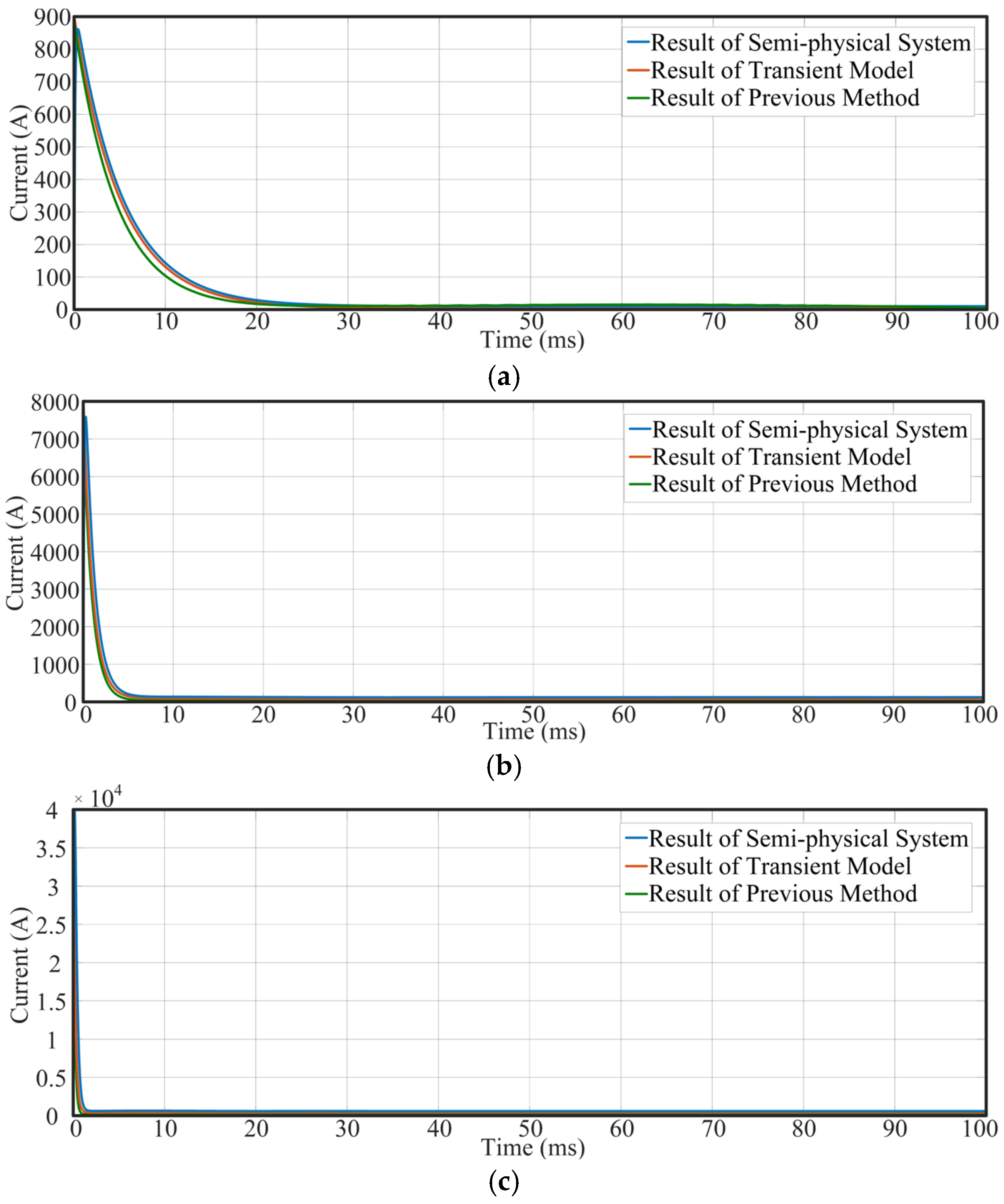
Figure 13 illustrates the fault output current i_dc1 of the generator component under various short-circuit resistances. The results are obtained from the semi-physical simulation test platform, the proposed transient modeling method, and the previous method. When a short-circuit fault occurs, i_dc1 rapidly rises to its peak value and subsequently decays gradually toward a steady state. The attenuation phase is mainly contributed by the discharge of the DC link capacitor, while the steady-state phase is influenced by the control system. This confirms the validity of the transient model mentioned above. At a fault resistance of 1 Ω, the peak current is approximately 900 A; at 0.1 Ω, it reaches approximately 7800 A; and at 0.01 Ω, it can reach up to approximately 40,000 A, clearly indicating a substantial increase in peak current as the fault resistance decreases.

Figure 13. The fault output current i_dc1 of the generator component. (a) R_f = 1 Ω, (b) R_f = 0.1 Ω, (c) R_f = 0.01 Ω.

The calculated results of the proposed transient model show a high similarity with the measured data from the semi-physical system. For normalization, the percentage error is used to quantify the similarity between results of simulation experiments, as defined in Equation (32).

$$\delta =\left|{\displaystyle \frac{x_{\mathrm{ev}}-x_{\mathrm{st}}}{x_{\mathrm{st}}}}\right|\times 100\%,$$

(32)

where δ denotes the percentage error of the measurement, x_ev is the measured value from the system under evaluation, and x_st is the corresponding value from the reference system. In this study, the systems under evaluation include the proposed transient model and the previous model, while the reference system refers to the semi-physical simulation system.

Under the fault resistance R_f of 1 Ω, the transient model yields a maximum error of 6.8% and an average error of 3.5%, in comparison to 9.0% and 6.0% for the previous method. At R_f = 0.1 Ω, the maximum and average errors of the transient model are 5.9% and 2.5%, respectively, while those of the previous method reach 8.9% and 4.5%. When the fault resistance is further reduced to 0.01 Ω, the transient model maintains a maximum error of 5.5% and an average error of 1.9%, while the previous method exhibits significantly higher errors, with a maximum of 8.0% and an average of 4.2%. These results clearly demonstrate that the proposed transient model achieves significantly higher accuracy than the previous method. Detailed error analysis is presented in Table 3.

Table 3. The error percentage of i_dc1 under different fault resistances.

Fault Resistance	Proposed Method		Previous Method
	Max	Average	Max	Average
1 Ω	6.8%	3.5%	9.0%	6.0%
0.1 Ω	5.9%	2.5%	8.9%	4.5%
0.01 Ω	5.5%	1.9%	8.0%	4.2%

2.

Verification of Transient Model for Fan Motor Component

Figure 14 illustrates the fault output current i_dc4 of the fan motor component under various short-circuit resistances, with results derived from the semi-physical simulation test platform, the proposed transient modeling method, and the previous method. When a short-circuit fault occurs, i_dc4 rapidly rises to its peak value and subsequently decays gradually toward zero. This confirms the validity of the transient model mentioned above. At a fault resistance of 1 Ω, the peak current is approximately 900 A; at 0.1 Ω, it reaches approximately 7800 A; and at 0.01 Ω, it can reach up to approximately 40,000 A, clearly indicating a substantial increase in peak current as the fault resistance decreases. This behavior closely parallels the dynamic response observed in the generator components under analogous fault conditions.

Figure 14. The fault output current i_dc4 of the fan motor component. (a) R_f = 1 Ω, (b) R_f = 0.1 Ω, (c) R_f = 0.01 Ω.

Under the fault resistance R_f of 1 Ω, the transient model yields a maximum error of 3.8% and an average error of 1.5%, in comparison to 9.0% and 3.6% for the previous method. At R_f = 0.1 Ω, the maximum and average errors of the transient model are 1.9% and 0.5%, respectively, while those of the previous method reach 4.9% and 1.5%. When the fault resistance is further reduced to 0.01 Ω, the transient model maintains a maximum error of 0.5% and an average error of 0.1%, while the previous method exhibits significantly higher errors, with a maximum of 2.0% and an average of 0.4%. These results clearly demonstrate that the proposed transient model achieves significantly higher accuracy than the previous method. A detailed error analysis is presented in Table 4.

Table 4. The error percentage of i_dc4 under different fault resistances.

Fault Resistance	Proposed Method		Previous Method
	Max	Average	Max	Average
1 Ω	3.8%	1.5%	9.0%	3.6%
0.1 Ω	1.9%	0.5%	4.9%	1.5%
0.01 Ω	0.5%	0.1%	2.0%	0.4%

3.

Verification of Transient Model for Power Battery Component

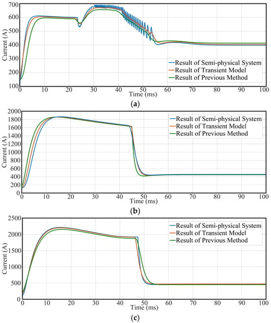
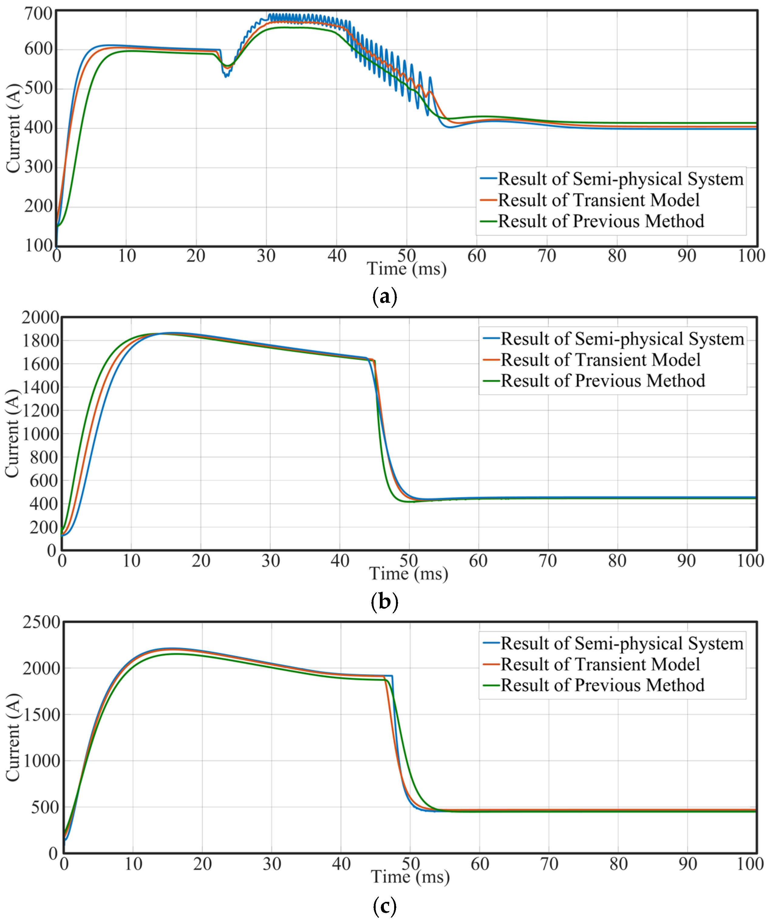
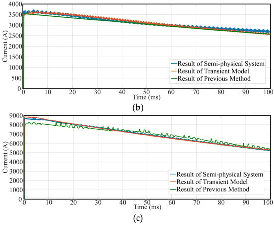
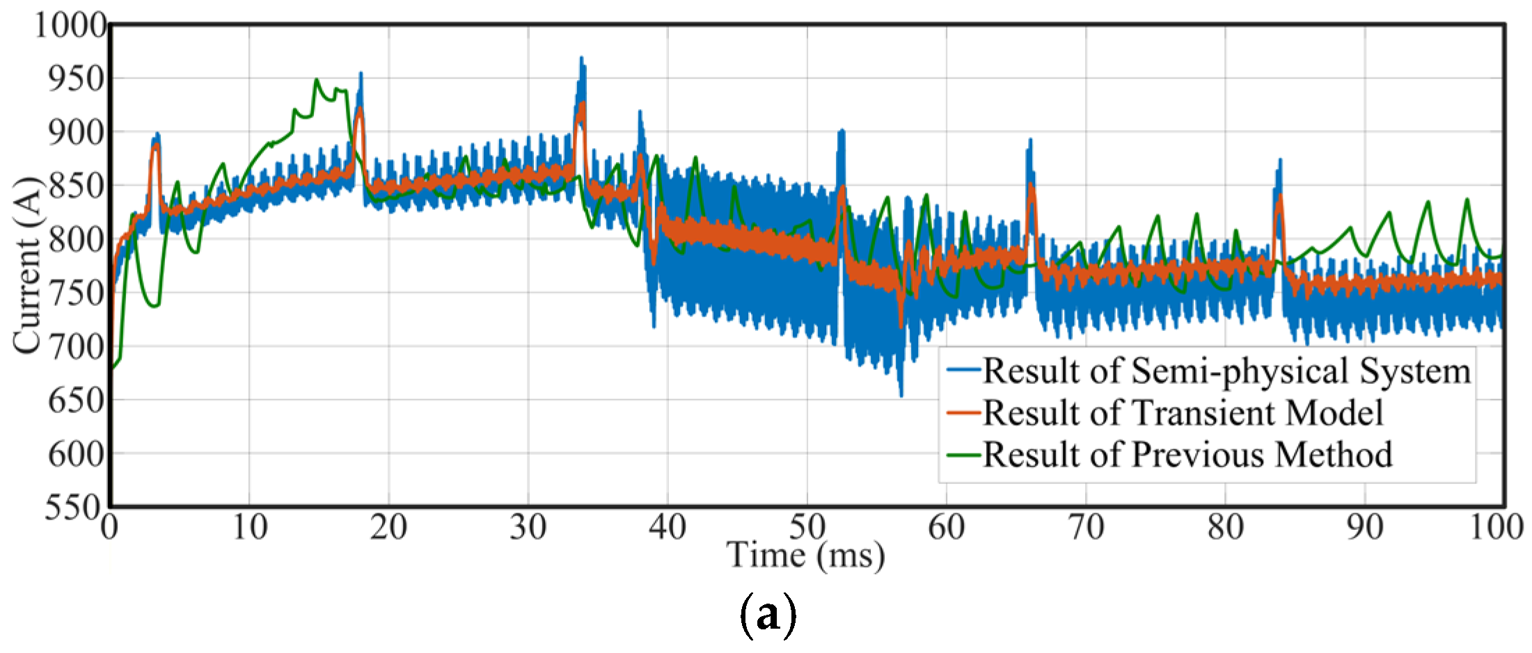
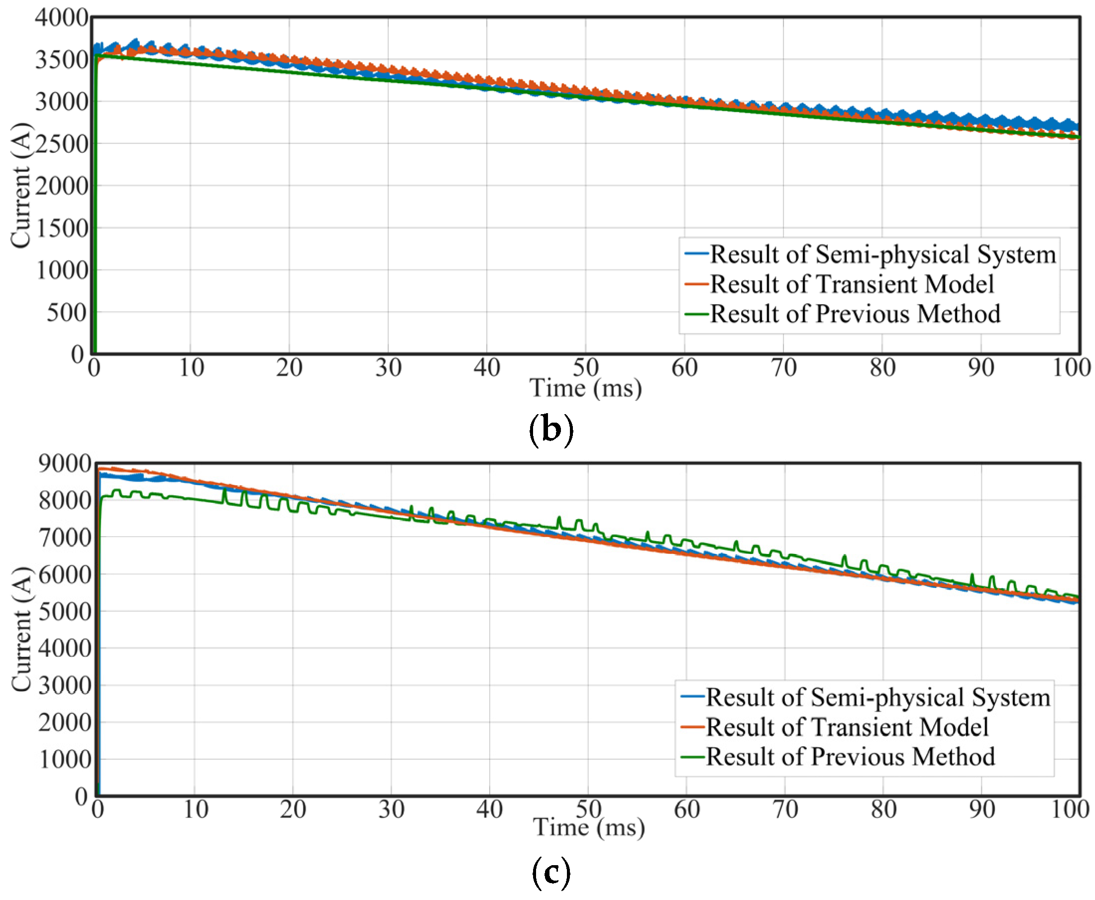
Figure 15 illustrates the fault output current i_dc2 of the power battery component under various short-circuit resistances, with results derived from the semi-physical simulation test platform, the proposed transient modeling method, and the previous method. When a fault occurs, i_dc2 rapidly rises to a high level, followed by decay toward a new steady-state value. A lower fault current leads to a shorter duration of the decaying phase and a more intense discharge from the power battery. The peak values of fault currents reach 690 A, 1850 A, and 2200 A under fault resistances of 1 Ω, 0.1 Ω, and 0.01 Ω, respectively.

Figure 15. The fault output current i_dc2 of the power battery component. (a) R_f = 1 Ω, (b) R_f = 0.1 Ω, (c) R_f = 0.01 Ω.

The calculated results of the proposed transient model show excellent agreement with the measured data from the semi-physical system. Under a fault resistance of 1 Ω, the maximum error percentage of the transient model is 4.3%, with an average of 2.3%, while the maximum error percentage of the previous method is 6.0%, with an average of 3.6%. At 0.1 Ω, the maximum and average errors are 3.3% and 1.9%, respectively, whereas those of the previous method are 5.2% and 2.5%. When the fault resistance is further reduced to 0.01 Ω, the transient model maintains errors as low as 1.8% (maximum) and 0.8% (average), while the previous method exhibits significantly higher deviations, reaching a maximum of 5.0% and an average of 2.1%. These results clearly demonstrate that the proposed transient model achieves substantially higher accuracy than the previous method. Detailed error analysis is provided in Table 5.

Table 5. The error percentage of i_dc2 under different fault resistances.

Fault Resistance	Proposed Method		Previous Method
	Max	Average	Max	Average
1 Ω	4.3%	2.3%	6.0%	3.6%
0.1 Ω	3.3%	1.9%	5.2%	2.5%
0.01 Ω	1.8%	0.8%	5.0%	2.1%

4.

Verification of Transient Model for DC Load Component

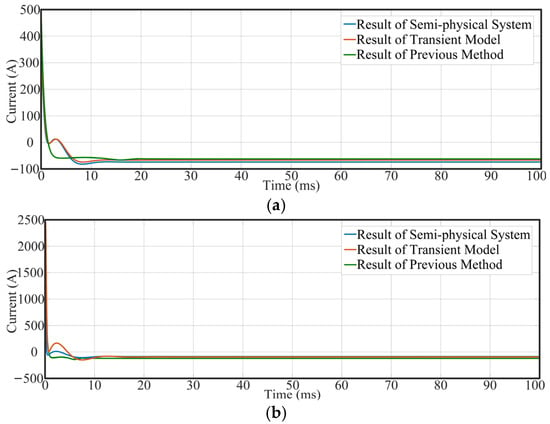
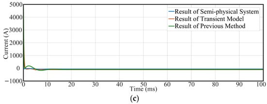
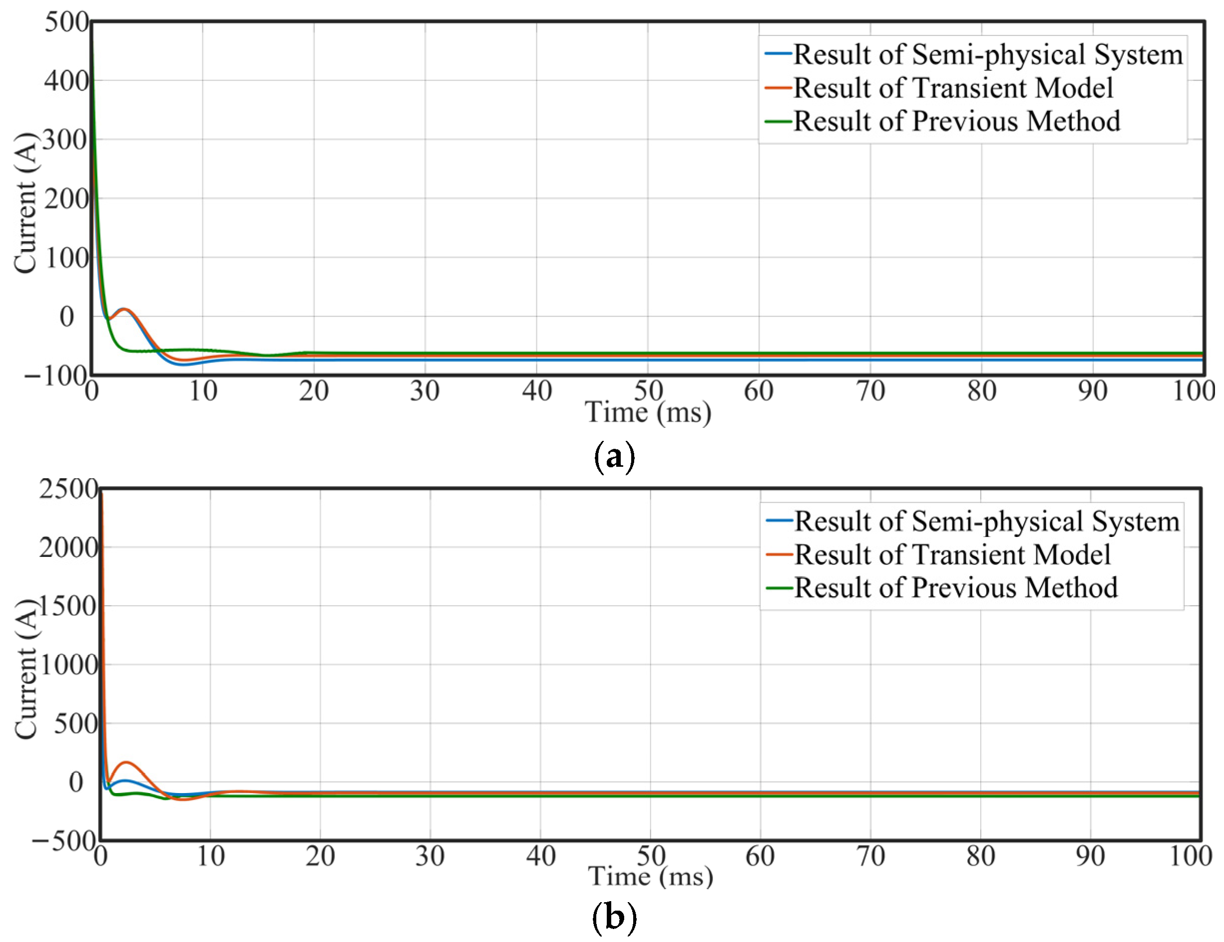
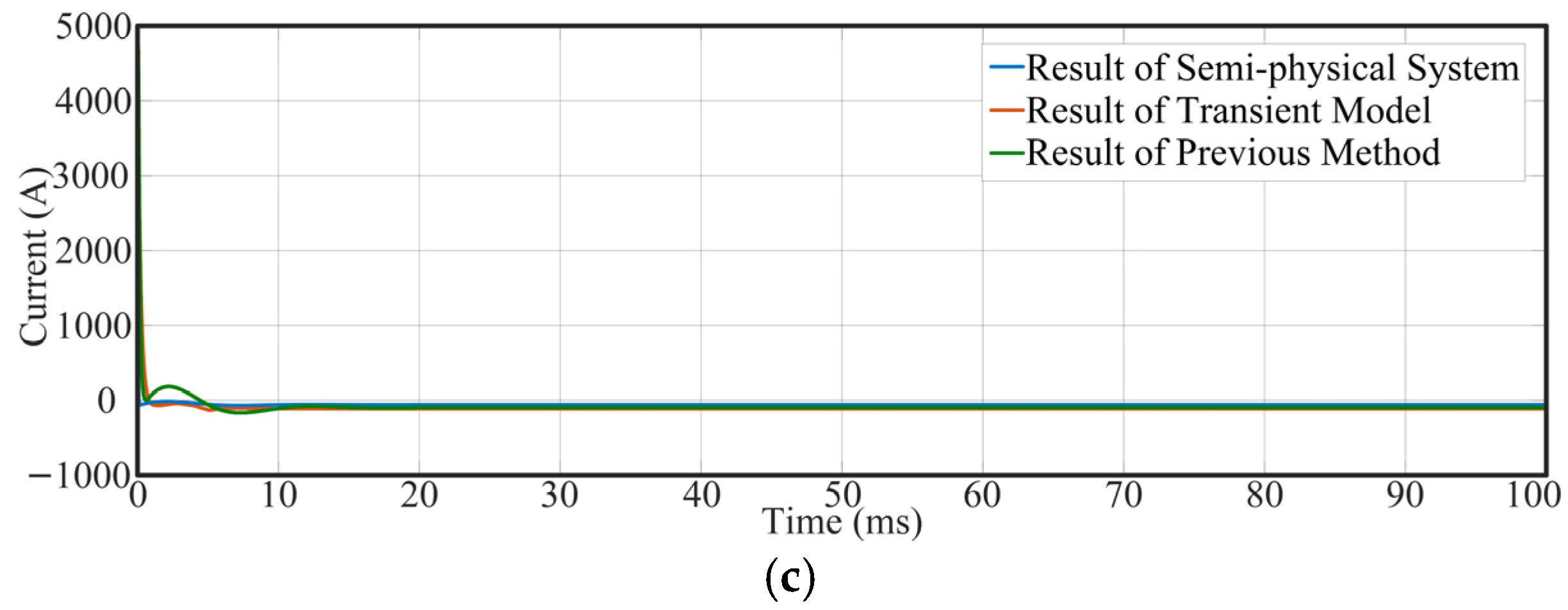
Figure 16 presents the fault output current i_dc3 of the DC load component under different short-circuit resistances. The results are from the semi-physical simulation test platform, the proposed transient modeling method, and the previous method. Certain differences can be observed among the i_dc3 waveforms generated by the three approaches. When a fault occurs, i_dc3 shows a characteristic transient response: it rapidly transitions from a negative value to a positive peak, followed by a gradual decay back into the negative region. Furthermore, the magnitude of this transient variation increases monotonically with fault severity.

Figure 16. The fault output current i_dc3 of the DC load component. (a) R_f = 1 Ω, (b) R_f = 0.1 Ω, (c) R_f = 0.01 Ω.

Under a fault resistance of 1 Ω, the maximum error percentage of the transient model is 3.6%, with an average of 1.7%, while that of the previous method is 10.3% with an average of 5.1%. At a fault resistance of 0.1 Ω, the corresponding maximum errors are 2.5% (transient model) and 9.7% (previous method), with average errors of 1.5% and 4.5%, respectively. At 0.01 Ω, the transient model achieves a maximum error of 1.9% and an average of 0.9%, while the previous method reaches 8.5% (maximum) and 3.6% (average). These results clearly demonstrate that the accuracy of the proposed transient model for the DC load component is significantly improved compared to the previous method. The detailed error analysis is provided in Table 6.

Table 6. The error percentage of i_dc3 under different fault resistances.

Fault Resistance	Proposed Method		Previous Method
	Max	Average	Max	Average
1 Ω	3.6%	1.7%	10.3%	5.1%
0.1 Ω	2.5%	1.5%	9.7%	4.5%
0.01 Ω	1.9%	0.9%	8.5%	3.6%

5.

Verification of Transient Model for Supercapacitor Component

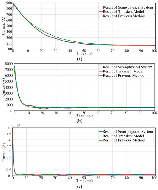
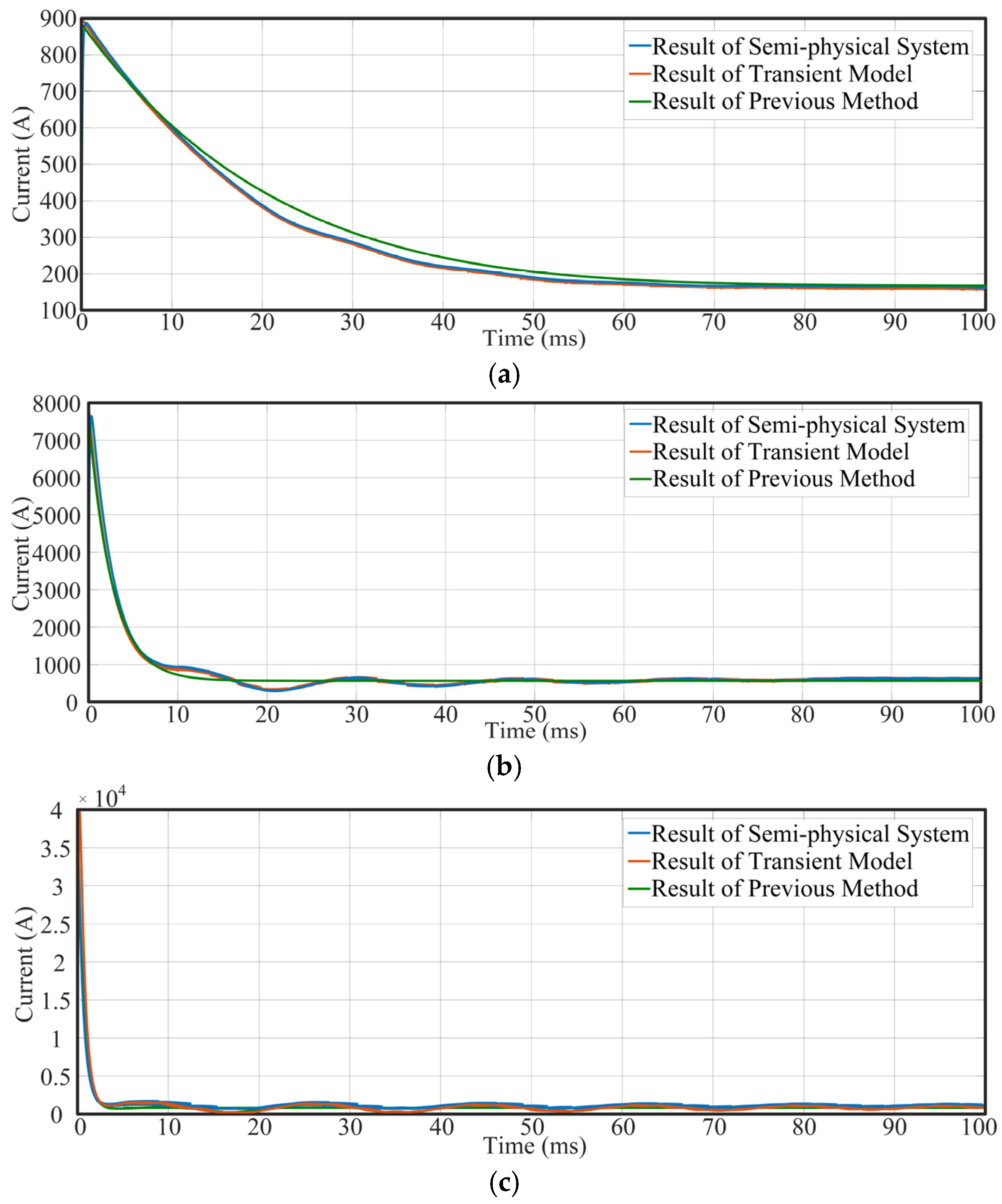
Figure 17 presents the fault output current i_sc of the supercapacitor component under different short-circuit resistances, with results obtained from the semi-physical simulation test platform, the proposed transient modeling method, and the previous method. Upon fault occurrence, i_sc rapidly rises to a peak value and subsequently decays gradually.

Figure 17. The fault output current i_sc of the supercapacitor component. (a) R_f = 1 Ω, (b) R_f = 0.1 Ω, (c) R_f = 0.01 Ω.

Owing to the strong instantaneous current output capability of the supercapacitor, i_sc remains at a high level throughout the simulation period. A lower fault resistance leads to a higher i_sc amplitude; where peak currents reach approximately 950 A, 3550 A, and 8800 A at fault resistances of 1 Ω, 0.1 Ω, and 0.01 Ω, respectively.

Notably, the transient model results show excellent agreement with those from the semi-physical system. At a fault resistance of 1 Ω, the transient model achieves a maximum error of 6.3% and an average error of 4.7%, compared to 9.7% (maximum) and 5.1% (average) for the previous method. At 0.1 Ω, the transient model yields maximum and average errors of 5.4% and 3.3%, respectively, while the previous method yields 8.8% and 4.5%. At 0.01 Ω, the transient model shows maximum and average errors of 4.1% and 2.2%, whereas the previous method shows 8.5% and 3.5%. These results clearly demonstrate that the proposed transient model for the supercapacitor component provides significantly improved accuracy over the previous method. The detailed error analysis is provided in Table 7.

Table 7. The error percentage of i_sc under different fault resistances.

Fault Resistance	Proposed Method		Previous Method
	Max	Average	Max	Average
1 Ω	6.3%	4.7%	9.7%	5.1%
0.1 Ω	5.4%	3.3%	8.8%	4.5%
0.01 Ω	4.1%	2.2%	8.5%	3.5%

6.

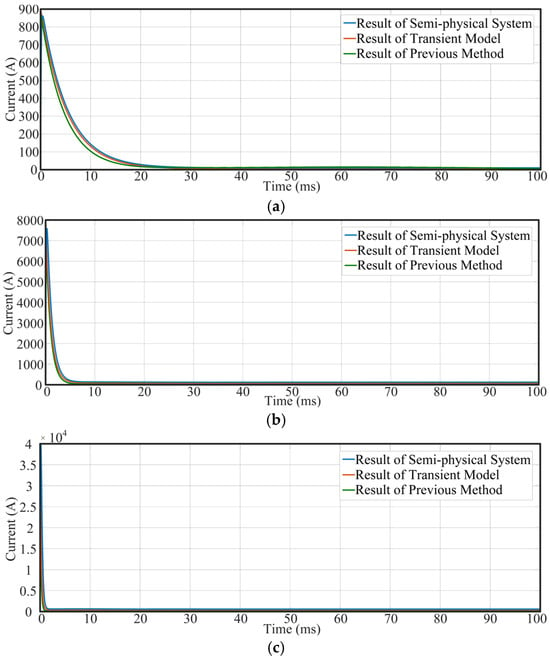
Verification of Transient Model for the Bus Voltage

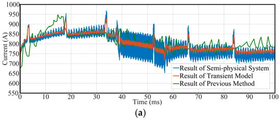
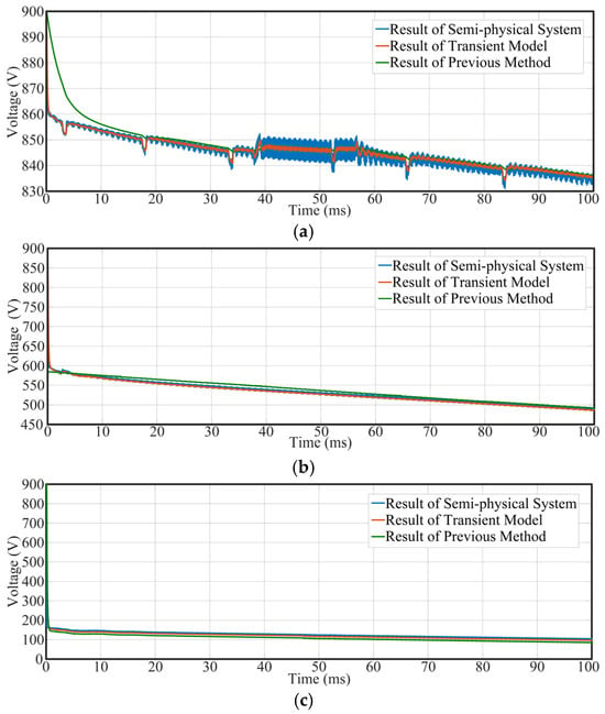
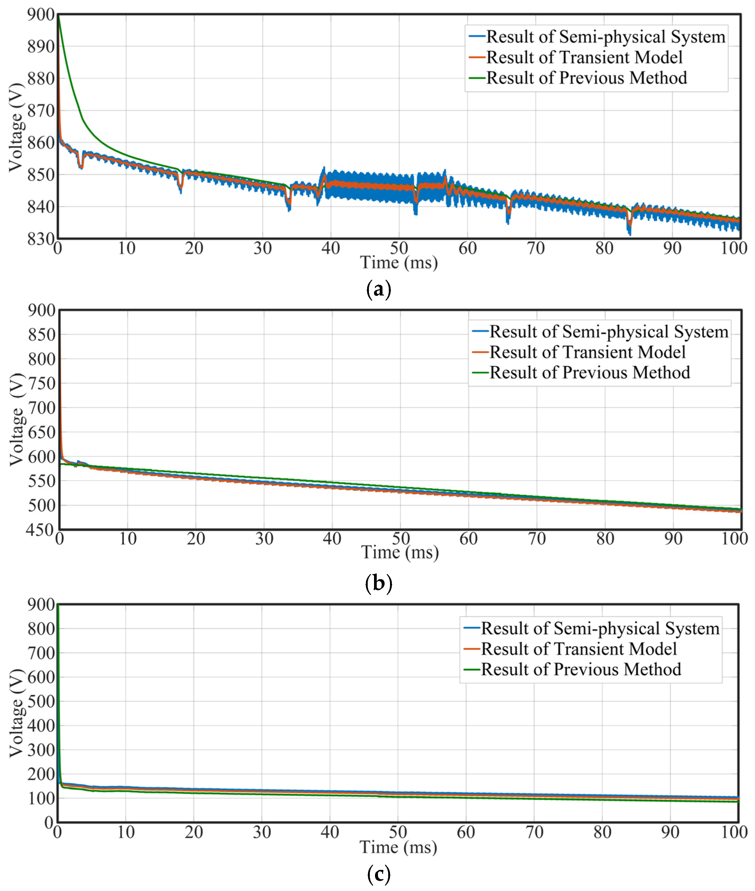
Figure 18 shows the bus voltage u_dc under different short-circuit resistance conditions. The results are from the semi-physical simulation test platform, the proposed transient modeling method, and the previous method. When a fault occurs, u_dc drops rapidly and gradually approaches a steady state. A lower fault resistance results in a faster bus voltage decline and a lower steady-state value; where the corresponding steady-state voltages are about 835 V, 490 V, and 100 V at fault resistances of 1 Ω, 0.1 Ω, and 0.01 Ω, respectively.

Figure 18. The bus voltage u_dc under a short-circuit fault. (a) R_f = 1 Ω, (b) R_f = 0.1 Ω, (c) R_f = 0.01 Ω.

In addition, the results obtained from the transient model are highly consistent with those from the semi-physical system. At a fault resistance of 1 Ω, the transient model achieves a maximum error of 1.2% and an average error of 0.6%, compared to 10.3% (maximum) and 5.5% (average) for the previous method. At 0.1 Ω, the transient model yields maximum and average errors of 0.9% and 0.5%, respectively, while the previous method yields 5.5% and 2.7%. At 0.01 Ω, the maximum and average errors of the transient model are 0.5% and 0.4%, whereas those of the previous method are 5.3% and 2.6%. These results clearly demonstrate that the proposed transient model for the bus voltage provides significantly improved accuracy compared to the previous method. The detailed error analysis is provided in Table 8.

Table 8. The error percentage of u_dc under different fault resistances.

Fault Resistance	Proposed Method		Previous Method
	Max	Average	Max	Average
1 Ω	1.2%	0.6%	10.3%	5.5%
0.1 Ω	0.9%	0.5%	5.5%	2.7%
0.01 Ω	0.5%	0.4%	5.3%	2.6%

5. Conclusions

This paper establishes a transient model of short-circuit faults in the HEA DC power system. In the proposed transient modeling method, the influence of control system on distributed power sources and load is taken into account, thereby improving the previous methods. Firstly, the transient characteristics of all components in the system are analyzed, including generators and fan motors, batteries and DC load, and supercapacitors. Subsequently, a comprehensive fault transient model of the HEA DC power system is established. Finally, the validity of the proposed method is verified through comparison with results from a semi-physical test platform. The results demonstrate that the proposed modeling approach enhances the accuracy of transient analysis for the faulty HEA DC power systems.

References

- Hasan, M.A.; Al Mamun, A.; Rahman, S.M.; Malik, K.; Al Amran, I.U.; Khondaker, A.N.; Reshi, O.; Tiwari, S.P.; Alismail, F.S. Climate Change Mitigation Pathways for the Aviation Sector. Sustainability 2021, 13, 3656. [Google Scholar] [CrossRef] [Scilit]
- Sayed, E.; Abdalmagid, M.; Pietrini, G.; Sa’Adeh, N.-M.; Callegaro, A.D.; Goldstein, C.; Emadi, A. Review of Electric Machines in More-/Hybrid-/Turbo-Electric Aircraft. IEEE Trans. Transp. Electrif. 2021, 7, 2976–3005. [Google Scholar] [CrossRef] [Scilit]
- Barzkar, A.; Ghassemi, M. Electric Power Systems in More and All Electric Aircraft: A Review. IEEE Access 2020, 8, 169314–169332. [Google Scholar] [CrossRef] [Scilit]
- Smita, S.; Pradeep, C.K. Analysis of the Propulsion System of an Electric Aircraft. Master’s Thesis, Chalmers University of Technology, Gothenburg, Sweden, 2023. [Google Scholar]
- Benzaquen, J.; He, J.; Mirafzal, B. Toward more electric powertrains in aircraft: Technical challenges and advancements. CES Trans. Electr. Mach. Syst. 2021, 5, 177–193. [Google Scholar] [CrossRef] [Scilit]
- Aboelezz, A.M.; Sedhom, B.E.; El-Saadawi, M.M.; Eladl, A.A.; Siano, P. State-of-the-Art Review on Shipboard Microgrids: Architecture, Control, Management, Protection, and Future Perspectives. Smart Cities 2023, 6, 1435–1484. [Google Scholar] [CrossRef] [Scilit]
- Lei, T.; Min, Z.; Gao, Q.; Song, L.; Zhang, X.; Zhang, X. The Architecture Optimization and Energy Management Technology of Aircraft Power Systems: A Review and Future Trends. Energies 2022, 15, 4109. [Google Scholar] [CrossRef] [Scilit]
- Siddavatam, A.K.R.; Rajashekara, K.; Huang, H.; Wang, F. Protection Coordination Strategy for the Distributed Electric Aircraft Propulsion Systems. World Electr. Veh. J. 2024, 15, 187. [Google Scholar] [CrossRef] [Scilit]
- Li, T.; Jiao, Z.; Wang, L.; Mu, Y. A Method of DC Arc Detection in All-Electric Aircraft. Energies 2020, 13, 4190. [Google Scholar] [CrossRef] [Scilit]
- Shu, H.; Hu, Y.; Lei, S.; Liang, B. A Novel Busbar Protection for LCC-VSC Hybrid MTDC Transmission System Based on Wavelet Packet Energy. IEEE Trans. Ind. Electron. 2025, 72, 4207–4217. [Google Scholar] [CrossRef] [Scilit]
- Feng, X.; Wang, B.; Wang, Z.; Hua, W.; Cheng, M. Diagnosis and Identification of Common Electrical Faults in PM Machine Drives. IEEE Trans. Power Electron. 2024, 39, 13686–13695. [Google Scholar] [CrossRef] [Scilit]
- Zhang, K.; Hu, X.; Liu, Y.; Lin, X.; Liu, W. Multi-fault Detection and Isolation for Lithium-Ion Battery Systems. IEEE Trans. Power Electron. 2022, 37, 971–989. [Google Scholar] [CrossRef] [Scilit]
- Ni, Q.; Luo, H.; Liu, J.; Zhan, Z.; Li, X.; Zhao, Z.; Lai, L.L. A Feature Vector Learning-Based Method for Diagnosing Main Circuit Ground Faults in Electrical Traction Drive Systems. IEEE Trans. Power Electron. 2024, 39, 2537–2545. [Google Scholar] [CrossRef] [Scilit]
- Zhang, Z.; Ren, J.; Tang, X.; Jing, S.; Lee, W.-J. Novel Approach for Arc Fault Identification with Transient and Steady State Based Time-Frequency Analysis. IEEE Trans. Ind. Appl. 2022, 58, 4359–4369. [Google Scholar] [CrossRef] [Scilit]
- Prince, S.K.; Kumar, D.; Affijulla, S.; Panda, G. Dominant/Lower Order Harmonic Injection Based Electric Fault Detection for DC Microgrids in Grid Coupled/Decoupled Scenarios. IEEE Trans. Ind. Appl. 2024, 60, 2542–2553. [Google Scholar] [CrossRef] [Scilit]
- Wang, T.; Liu, W.; Hao, Z. A Decentralized Model-Based Fault Detection and Isolation Scheme for MVDC Shipboard Power Systems. IEEE Trans. Transp. Electrif. 2024, 10, 7804–7815. [Google Scholar] [CrossRef] [Scilit]
- Prince, S.K.; Affijulla, S.; Panda, G. Protection of DC Microgrids Based on Complex Power During Faults in On/Off-Grid Scenarios. IEEE Trans. Ind. Appl. 2023, 59, 244–254. [Google Scholar] [CrossRef] [Scilit]
- Yu, Z.; Wang, X.; Fang, M.; Zhang, S. Research on Cable Fault Online Monitoring and Localization System Based on Time-Frequency Reflectometry. In Proceedings of the 2024 International Conference on Advances in Electrical Engineering and Computer Applications (AEECA), Dalian, China; IEEE: Piscataway, NJ, USA, 2024; pp. 189–193. [Google Scholar] [CrossRef] [Scilit]
- Cui, H.; Tu, N. HVDC transmission line fault localization base on RBF neural network with wavelet packet decomposition. In Proceedings of the 2015 12th International Conference on Service Systems and Service Management (ICSSSM), Guangzhou, China; IEEE: Piscataway, NJ, USA, 2015; pp. 1–4. [Google Scholar] [CrossRef] [Scilit]
- Yang, Z.; Zhang, H.; Li, N.; Wang, Z. Research on Fault Localization Method of Flexible Distribution System Based on Deep Learning. In Proceedings of the 2024 9th Asia Conference on Power and Electrical Engineering (ACPEE), Shanghai, China; IEEE: Piscataway, NJ, USA, 2024; pp. 1549–1553. [Google Scholar] [CrossRef] [Scilit]
- Jiufu, W.; Li, B. A Novel Surge Suppression Scheme for Capacitive Pulsed Power Supply. IEEE Trans. Plasma Sci. 2022, 50, 2396–2402. [Google Scholar] [CrossRef] [Scilit]
- Domoto, K.; Ninomiya, T.; Ishizuka, Y.; Simanjorang, R.; Yamaguchi, H.; Abe, S.; Kaga, M. Surge snubber design for high power-density DC-DC converters in HVDC power distribution systems. In Proceedings of the 2012 International Conference on Renewable Energy Research and Applications (ICRERA), Nagasaki, Japan; IEEE: Piscataway, NJ, USA, 2012; pp. 1–5. [Google Scholar] [CrossRef] [Scilit]
- Zhang, Z.; Wang, H.; Wang, K.; Zhao, Y. Contribution Mechanism and Impact Analysis of AC System at the Diode Natural Commutation and Conduction Stage During Bipolar Short-Circuit Fault for Single-Terminal VSC-Based DC Distribution Networks. IEEE Access 2022, 10, 74082–74102. [Google Scholar] [CrossRef] [Scilit]
- Pourmirasghariyan, M.; Zarei, S.F.; Hamzeh, M.; Blaabjerg, F. A Power Routing-Based Fault Detection Strategy for Multi-Terminal VSC-HVDC Grids. IEEE Trans. Power Deliv. 2023, 38, 528–540. [Google Scholar] [CrossRef] [Scilit]
- Chapparya, V.; Dey, A.; Rodriguez, J.; Garcia, C. Switch Failure Detection and Identification Using Diode Current for Single-Switch DC–DC Converters. IEEE J. Emerg. Sel. Top. Power Electron. 2025, 13, 4976–4986. [Google Scholar] [CrossRef] [Scilit]
- Hu, Y.; Li, Z.; Zhao, C.; Li, Y. Characteristics Analysis and Design of a Resonant dc–dc Converter with ZCS and Short-Circuit Fault Current Limiting Capability. IEEE J. Emerg. Sel. Top. Power Electron. 2022, 10, 2223–2232. [Google Scholar] [CrossRef] [Scilit]
Disclaimer/Publisher’s Note: The statements, opinions and data contained in all publications are solely those of the individual author(s) and contributor(s) and not of MDPI and/or the editor(s). MDPI and/or the editor(s) disclaim responsibility for any injury to people or property resulting from any ideas, methods, instructions or products referred to in the content. |
© 2026 by the authors. Licensee MDPI, Basel, Switzerland. This article is an open access article distributed under the terms and conditions of the Creative Commons Attribution (CC BY) license.