


Abstract
Laminar separation bubbles (LSBs) on low-Reynolds-number airfoils are sustained by intrinsic unsteadiness driven by Kelvin–Helmholtz (K-H) growth in the separated shear layer. Using incompressible 2D URANS with the SA- transition model for a NACA 0012 airfoil at , we reveal that numerical dissipation behaves as a critical bifurcation parameter. Validated against the recent Jardin (2025) experimental benchmark, the physical state correctly resolves the LSB-induced pressure plateau () and local negative skin friction (). However, when numerical dissipation exceeds the K-H instability growth rate, the physical limit-cycle oscillation collapses into a spurious fixed-point attractor—a phenomenon defined as numerical quenching. This pseudo-convergence triggers a catastrophic ∼30% deficit in mean lift (). Furthermore, at , a drag-mechanism inversion is identified: while the physical branch is dominated by LSB-induced pressure (form) drag, the quenched branch exhibits a non-physical drag surge that exceeds the fully turbulent baseline. Phase portraits and power spectral densities () provide objective diagnostics, demonstrating that standard residual convergence is a deceptive indicator of physical fidelity in transitional separated aerodynamics.
1. Introduction
1.1. Low-Reynolds-Number Laminar Separation Bubbles and Intrinsic Unsteadiness
Transitional airfoil flows at exhibit a delicate competition between viscous diffusion, adverse pressure gradients, and shear-layer instability. This Reynolds-number range arises in several settings, including small-scale flight, the thin Martian atmosphere, and bio-inspired micro-air vehicles [1,2,3,4]. The aerodynamic performance in this regime is of critical importance for the development of unconventional rotorcraft, such as the Mars Helicopter and future planetary exploration platforms [5,6,7,8,9,10]. While these applications motivate the study, the underlying mechanisms are generic to low- external aerodynamics [11,12].
The hallmark of this regime is the Laminar Separation Bubble (LSB), a complex topology involving laminar separation, transition via Kelvin–Helmholtz amplification in the separated shear layer, and turbulent reattachment [13,14,15,16,17]. The dynamic behavior of the LSB—its formation, migration, and bursting—introduces strong nonlinearities in aerodynamic loads, including lift dead-bands, hysteresis, and abrupt stall characteristics [18,19,20,21].
The present work focuses on a controlled airfoil benchmark that matches recent low-speed experimental datasets [22] and established measurements [23]. The objective is to isolate transitional LSB physics and numerical behavior at conditions where the incompressible assumption is appropriate [24]. While three-dimensional effects such as stall cells eventually modulate the bubble topology, the inception of the collapse is a fundamental competition between the solver’s dissipation and the 2D shear-layer instability, justifying a focused 2D study.
1.2. The Dilemma of Transition Modeling: Physical Instability vs. Numerical Stability
Given the prohibitive computational cost of Direct Numerical Simulation (DNS) [25,26] and the grid-resolution requirements of Large Eddy Simulation (LES) [27] for parametric studies, Reynolds-Averaged Navier-Stokes (RANS) approaches remain widely used [28]. However, the “predictability crisis” in low- flows stems from the failure of fully turbulent models (e.g., Spalart–Allmaras) to capture the laminar portion of the LSB, leading to gross over-prediction of drag and under-prediction of lift [23,29,30]. While integral methods such as XFOIL [31] provide rapid estimates, they often struggle with the strong unsteadiness and massive separation characteristic of the pre-stall regime [32].
To bridge this gap, correlation-based transition models have been developed. However, multi-equation frameworks, such as the four-equation model, introduce significant complexity. They rely on non-local variables and intricate empirical correlations that often result in numerical stiffness, particularly when coupled with the highly non-linear source terms required to trigger transition rapidly inside a short separation bubble [30,33,34]. This “stiffness” frequently leads to convergence stagnation or requires extremely small time-steps, complicating RANS-based simulation workflows.
In response, single-equation transition models, such as the SA- model developed by Bas and Cakmakcioglu [35], have gained traction. By solving a single transport equation for intermittency coupled with the robust SA turbulence model, the SA- framework offers a balance between physical fidelity and computational efficiency. Recent studies have applied correlation-based transition models to a range of configurations [33,34,36], yet their numerical resilience in unsteady LSB shedding remains under-explored. While the general limitations of RANS in LSB prediction are documented [36,37], the specific mechanism of numerical quenching leading to a non-conservative drag crossover remains unreported. This study fills this gap by identifying how numerical dissipation triggers a topological bifurcation in the solution space.
1.3. The Numerical Stability–Fidelity Paradox
A critical, yet often overlooked, aspect of simulating transitional flows is the interplay between numerical dissipation and physical instability. In the linear lift regime () of a NACA 0012 airfoil at , the flow is inherently unsteady, characterized by the periodic shedding of vortices from the LSB (Limit Cycle Oscillations, LCO) [18,38].
Here lies a fundamental conflict, which we term the “Stability-Fidelity Paradox.” From a numerical perspective, implicit solvers introduce numerical dissipation (via upwind discretization or temporal integration) to suppress oscillations and drive residuals to machine zero [39]. However, from a physical perspective, suppressing these oscillations is equivalent to attenuating the Kelvin–Helmholtz instabilities that sustain reattachment [40]. Recent theoretical work suggests that excessive numerical dissipation can trigger a bifurcation in the solution space, causing the flow to jump from a physically correct unsteady state to a spurious steady attractor [41,42,43]. We define this process of artificial stabilization as “numerical quenching,” which results in a physically erroneous pseudo-steady state that satisfies standard convergence criteria while yielding incorrect aerodynamic coefficients. We specifically focus on the “drag mechanism inversion” phenomenon, where LSB-induced form drag competes with and can exceed fully turbulent baselines.
To make these terms operational and falsifiable, we define an aerodynamic state vector
its time-mean over a sampling window as
and the limit-cycle content as
We classify the solution as a physically unsteady LSB state when is finite and the spectrum of exhibits a distinct dominant peak at a Strouhal number consistent with shear-layer shedding [44]. Conversely, we define the pseudo-steady state as the simultaneous collapse of the - phase-space attractor toward a fixed-point attractor and the disappearance of the characteristic Strouhal peak in the energy spectrum [44,45]. We emphasize that this pseudo-steady state is a mathematically valid solution to the discretized equations (a fixed point of the numerical map), even if it is physically incorrect. Within this framework, numerical quenching denotes the bifurcation event in which numerical dissipation introduces an effective decay rate that overwhelms Kelvin-Helmholtz amplification, driving the limit-cycle attractor toward a fixed-point attractor [45].
1.4. Objectives and Scope
This study aims to clarify how numerical dissipation competes with intrinsic LSB instabilities in correlation-based transition modeling. Using the NACA 0012 airfoil at as a benchmark, validated against high-fidelity experiments [22,23], we address three specific gaps:
- Quantification of numerical quenching: We identify objective diagnostics for the collapse of a physical limit-cycle attractor to a spurious fixed point using phase portraits and spectral signatures.
- Interpretation as a dynamical transition: We connect the observed collapse to an inverse Hopf-like process in which numerical dissipation suppresses the unstable shear-layer mode that sustains the LSB.
- Mechanism of drag inversion: We relate the drag response to boundary-layer and wake topology, emphasizing the partition between pressure (form) and viscous contributions.
By dissecting these mechanisms, this work provides a dynamical-systems framing for interpreting when the SA- closure preserves the physical LSB attractor and when it collapses to a spurious steady branch.
While multi-equation transition frameworks (e.g., ) are widely used, this work focuses exclusively on the SA- formulation to isolate the interplay between source-term stiffness, grid topology, and numerical dissipation that is most pronounced in single-equation intermittency closures; an across-model benchmarking campaign is intentionally left outside the present scope.
2. Numerical Methodology
2.1. Governing Equations and the URANS Framework
The unsteady flow field is governed by the incompressible Unsteady Reynolds-Averaged Navier-Stokes (URANS) equations. While DNS remains the gold standard for resolving the full spectrum of turbulent scales [25], its computational cost scales as , rendering it impractical for parametric studies. Consequently, this study employs the URANS approach coupled with a correlation-based transition model to balance physical fidelity and computational cost. The incompressible formulation is adopted to remain consistent with the low-speed experimental benchmarks used for validation and to isolate transitional LSB dynamics from compressibility effects [22,23,24].
The conservation of mass and momentum are expressed as:
where the Reynolds stress tensor is modeled using the Boussinesq hypothesis:
Here, represents the eddy viscosity, which is the primary variable computed by the turbulence model. In this study, the Spalart-Allmaras (SA) one-equation model [46] is selected as the baseline due to its robustness in aerospace applications and its numerical stability compared to two-equation ( or ) models in external aerodynamics.
2.2. The SA- Transition Model
To capture the laminar–turbulent transition process, specifically the LSB dynamics at , the baseline SA model is augmented with the single-equation transition model [35]. The model solves a transport equation for the intermittency factor , which locally scales the production term of the eddy viscosity. The transport equation for the intermittency is given by [35]:
where and are the transition source and destruction terms, respectively, controlled by critical Reynolds number correlations. The coupling with the Spalart-Allmaras turbulence model is achieved by modifying the production term as . This ensures that the eddy viscosity production is suppressed in the laminar region () and activated in the turbulent region (). Detailed discussions on the numerical convergence characteristics are provided in Section 3.1. The spatial resolution of the transition front is critical for the conditioning of the implicit linear system. Based on the mesh sensitivity analysis conducted, a fine mesh of 188k cells is adopted. It is important to note that the fidelity gap observed in coarser settings is primarily a model formulation issue (stiffness of the single-equation closure) rather than a simple grid convergence issue. All model constants for the SA- formulation are kept at their default values as implemented in the solver, ensuring the results are representative of standard application practices.
2.3. Numerical Implementation and Discretization
The simulations were performed using the finite-volume solver Simcenter STAR-CCM+ (Version 2510). The specific numerical schemes were chosen to minimize numerical dissipation, which is identified as the primary culprit in the “Stability-Fidelity Paradox.” To ensure statistical stationarity, the simulations were conducted in two phases. First, the flow was advanced for 150 convective time units () to wash out initial transients. Subsequently, time-averaged aerodynamic coefficients were collected over a sampling window of 400 . With a characteristic shedding Strouhal number , the dominant shedding period is , and the sampling window therefore encompasses approximately 80 shedding cycles. This duration was verified to be sufficient for the mean lift and drag values to converge within 0.1%.
- Spatial Discretization: A second-order upwind scheme is used for the convective fluxes of momentum and turbulence scalars. While stable, upwind schemes introduce inherent numerical diffusion [47,48]. To mitigate this, the grid is strictly aligned with the flow direction in the wake region (C-grid topology).
- Temporal Discretization: A second-order implicit dual-time stepping scheme is employed [49]. The physical time step is set to s. This temporal resolution is selected to capture the dominant LSB shear-layer shedding () while mitigating excessive damping by the implicit time integration. The adequacy of is confirmed by the time-step independence study in Section 2.6.
- Pressure-Velocity Coupling: The SIMPLEC algorithm is utilized for its superior convergence rates in unsteady flows compared to PISO or SIMPLE [47].
- Computational Platform: All simulations were performed using Simcenter STAR-CCM+ (Version 2510) with its GPU-accelerated implementation on workstation-class hardware.
2.4. Computational Domain and Grid Topology
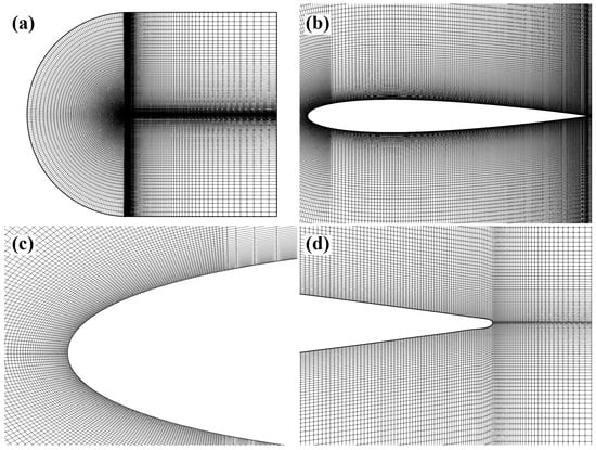
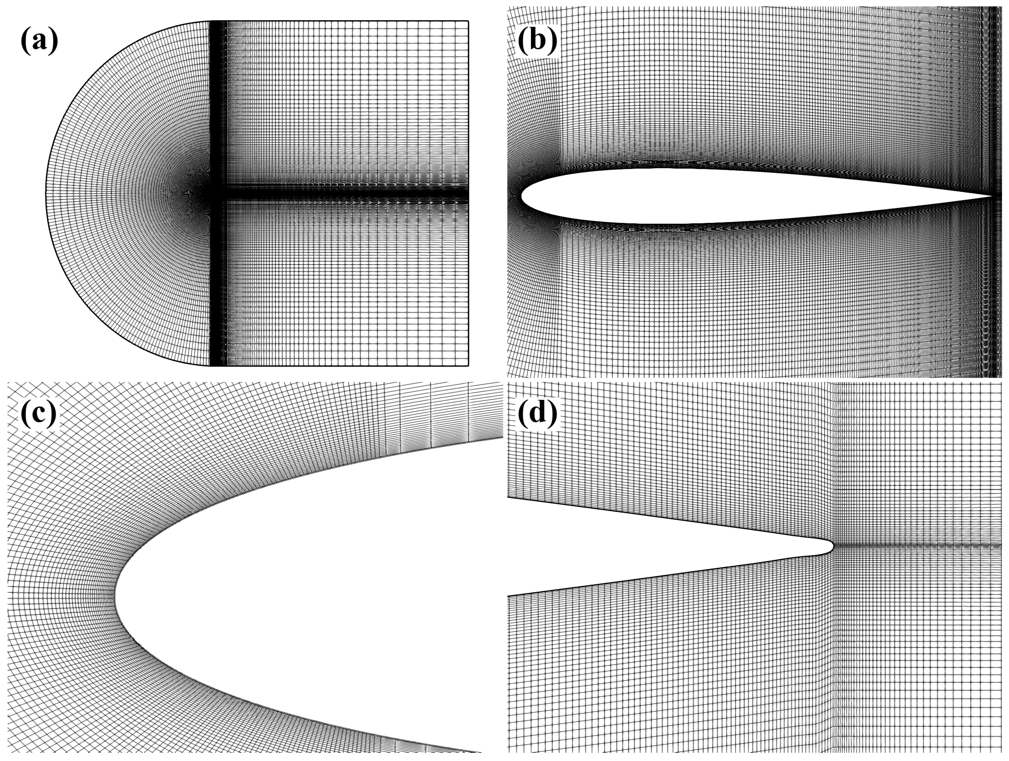
To eliminate far-field boundary effects, a C-grid topology is constructed with the outer boundary extending 50 chord lengths () from the airfoil, as shown in Figure 1. The domain is discretized using a structured quadrilateral mesh to ensure high orthogonality (minimum angle ) and low skewness. The far-field boundary is set as a velocity inlet with a turbulence intensity of , matching the experimental environment.
Figure 1.
Structured C-grid topology for the NACA 0012 airfoil: (a) global computational domain; (b) mesh distribution around the airfoil; (c) magnified view of the leading edge; (d) trailing edge and wake refinement. Representative structured mesh (188 k cells) used for production runs.
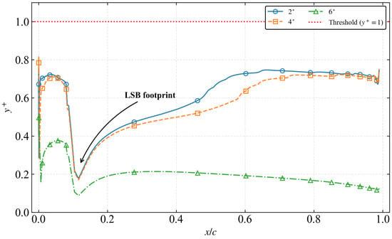
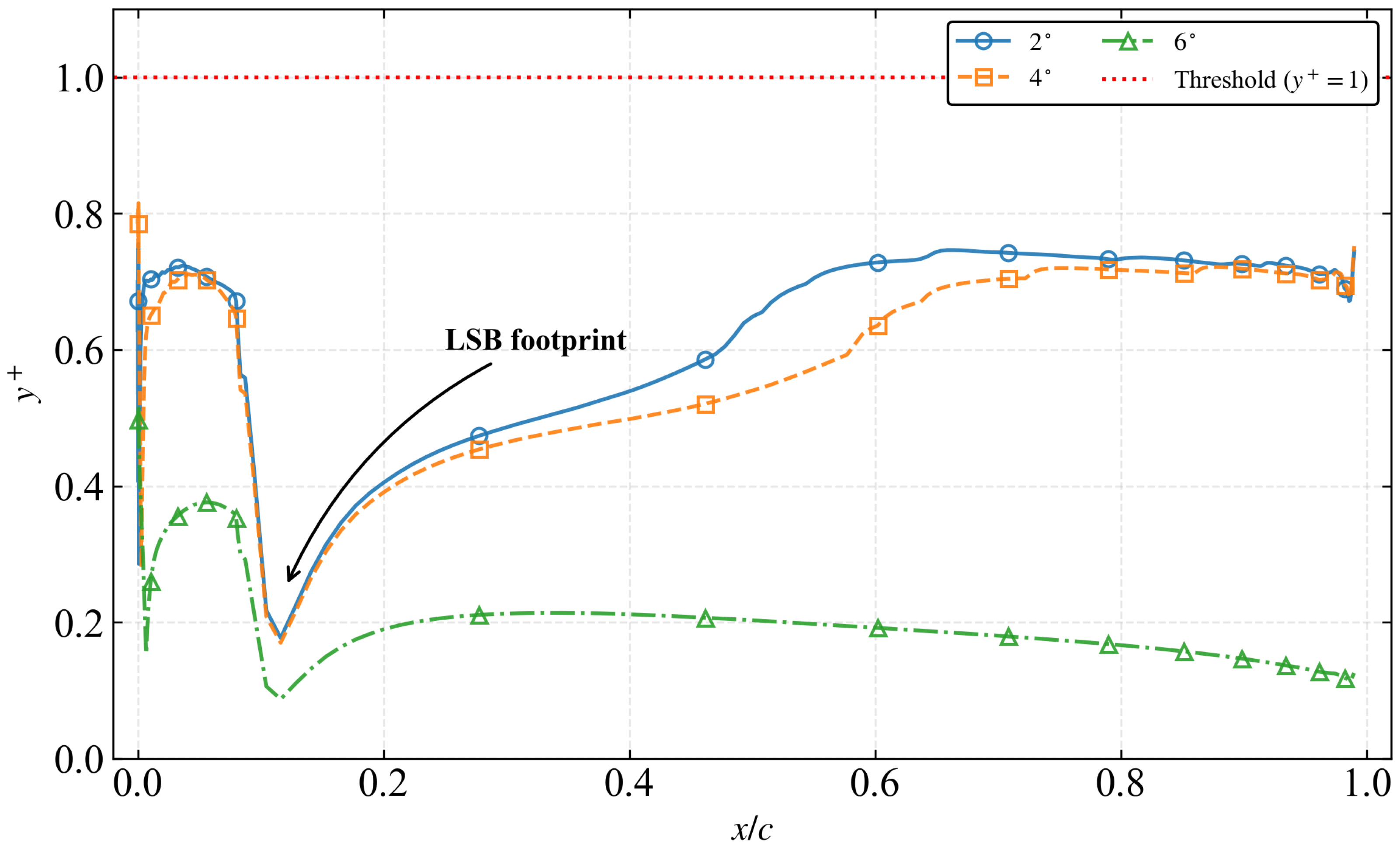
- Near-Wall Resolution: To resolve the viscous sublayer and the critical onset of the LSB, the first cell height is set to , ensuring a dimensionless wall distance across the entire suction surface for all angles of attack (Figure 2).
- Streamwise Resolution: The grid is heavily clustered in the leading-edge region () and the potential separation zone. The fine mesh (188k cells) maintains a streamwise spacing of in the transition region, which is critical for the smooth activation of the intermittency source terms.
Figure 2.
Chordwise distribution of the wall-normal dimensionless distance on the suction surface. The threshold is maintained for all investigated angles of attack to ensure viscous sublayer resolution.
It is important to clarify the scope of the current two-dimensional study. While many practical configurations are inherently three-dimensional, this work intentionally focuses on a 2D airfoil section to isolate the interaction between transition-model source terms, numerical dissipation, and the intrinsic LSB instability without additional spanwise dynamics. The 2D framework provides a controlled numerical laboratory for diagnosing pseudo-convergence and numerical quenching and for establishing phase-space and spectral diagnostics that can be transferred to more complex three-dimensional configurations.
2.5. Near-Wall Resolution and Viscous Sublayer Analysis
The accuracy of the SA- transition model is heavily predicated on the resolution of the wall-normal velocity gradients, as the intermittency production terms are calculated by integrating directly through the viscous sublayer without the use of wall functions [50]. Figure 2 illustrates the chordwise distribution of the dimensionless wall distance for the suction surface across the investigated range of angles of attack.
It is observed that remains strictly below 0.8 for all cases, with the maximum values occurring near the suction peak at . A characteristic “numerical footprint” of the LSB is clearly visible at , where the values exhibit a localized dip. This phenomenon is physically consistent with the reduction in wall shear stress () within the separation bubble, as and . The fact that remains well within the required threshold even under the most demanding unsteady conditions ensures that the boundary layer thickness and the subsequent transition inception are resolved with high physical fidelity.
2.6. Verification and Validation Strategy
A rigorous Verification and Validation (V&V) process is conducted following established best practices [37,51]:
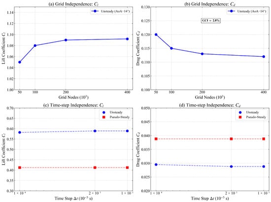
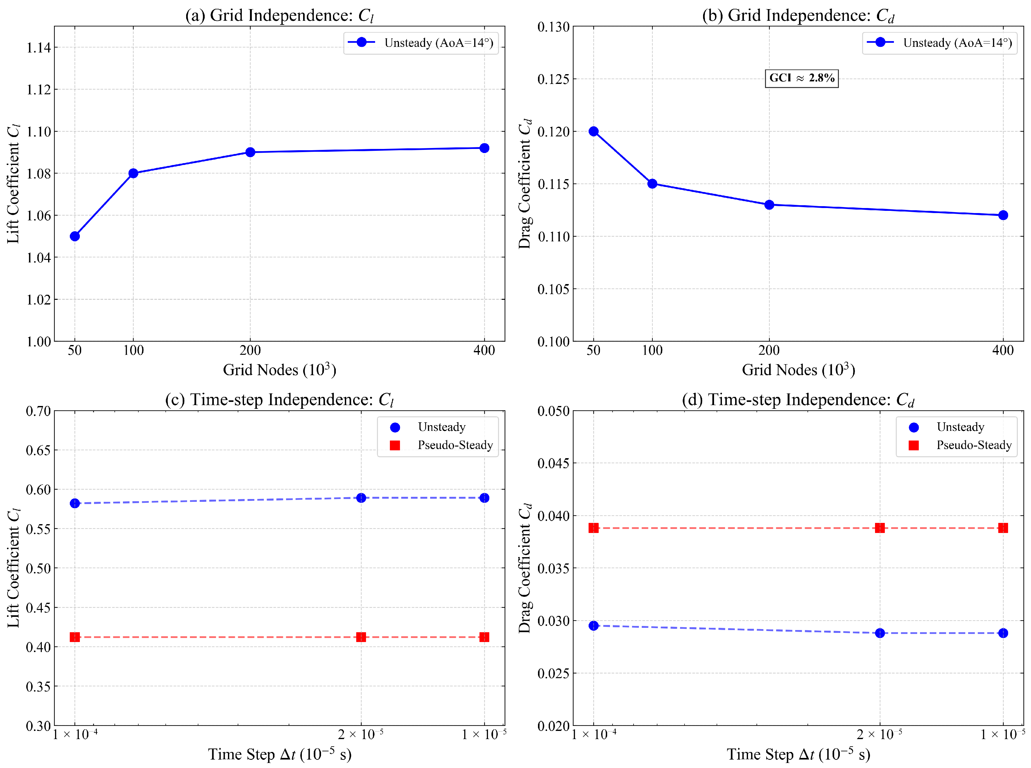
- Grid Independence: Three grid levels (Coarse: 60 k, Medium: 97 k, Fine: 188 k) are evaluated. The Grid Convergence Index (GCI) is calculated to quantify discretization error (Table 1 and Figure 3).Table 1. Grid independence study summary at and .Figure 3. Spatial and temporal independence study for the SA- model: (a) grid sensitivity of at ; (b) grid sensitivity of at ; (c) time-step sensitivity of at ; (d) time-step sensitivity of at .
- Time-Step Independence: The sensitivity of the LCO amplitude to is assessed at to ensure the “Drag Mechanism Inversion” is a physical phenomenon rather than a temporal artifact.
- Experimental Validation: The numerical results are validated against the high-fidelity datasets of Jardin et al. and Tank et al., focusing on both integral forces () and distributed surface data ().
As summarized in Table 1 and Figure 3a,b, the lift and drag coefficients exhibit a monotonic convergence behavior. To quantify the numerical uncertainty, the GCI was calculated according to established procedures [52,53]. The for the lift coefficient between the medium and fine grids is found to be 0.42%, which is well within the asymptotic range of convergence. Although the relative deviation between the medium and fine meshes is approximately 2.5%, this margin is considered acceptable. The primary objective of this study lies in capturing the topological bifurcation (numerical quenching) (rather than the absolute minimization of drag discretization error), and the LCO frequencies (), which are consistently resolved by both the medium and fine meshes. Thus, the 188k mesh is robustly sufficient to support the physical conclusions of the “Stability-Fidelity Paradox.”
Temporal independence was subsequently verified at the stability boundary () by varying the time step from s to s. As shown in Figure 3c,d, the time-averaged force coefficients and the primary Strouhal number of the LCO remain invariant for s. This confirms that the selected temporal resolution is robust enough to resolve the finest energy-containing scales of the shear-layer instability. Consequently, the 188 k mesh and an ultra-fine time step of s were adopted for all production simulations.
3. Results and Discussion
3.1. Grid Independence and Computational Efficiency
A systematic grid independence study was conducted using three mesh levels (Coarse: 60 k, Medium: 97 k, Fine: 188 k). As summarized in Table 1 and Figure 3, the aerodynamic coefficients converge asymptotically. To quantify the discretization error, the Grid Convergence Index (GCI) was calculated following the methodology of Roache [54]. Using the Richardson extrapolation with a safety factor of , the GCI for the fine mesh is estimated to be approximately for and for . Although the error slightly exceeds the target , this margin is considered acceptable given that the primary objective is to capture the topological bifurcation rather than absolute drag minimization. In this configuration, grid coarsening also provides a practical proxy for increased numerical dissipation in the separation shear layer and wake. In addition to monotonic convergence of the time-averaged loads, the SA- closure exhibits a pronounced stiffness sensitivity when the intermittency activation region is under-resolved. The medium mesh lies near a stiffness peak, where sharply localized intermittency source terms degrade the conditioning of the implicit update. Refining to the 188k mesh regularizes these source-term gradients, improving conditioning and enabling consistent deep convergence within each physical time step. Consequently, the 188k mesh was selected for all production runs to ensure physical fidelity and numerical robustness in the presence of intrinsic LSB unsteadiness.
3.2. Global Aerodynamic Performance and Validation
3.2.1. Lift Characteristics and the High-Fidelity Linear Regime
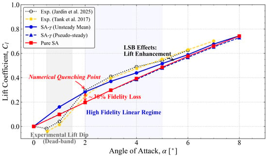
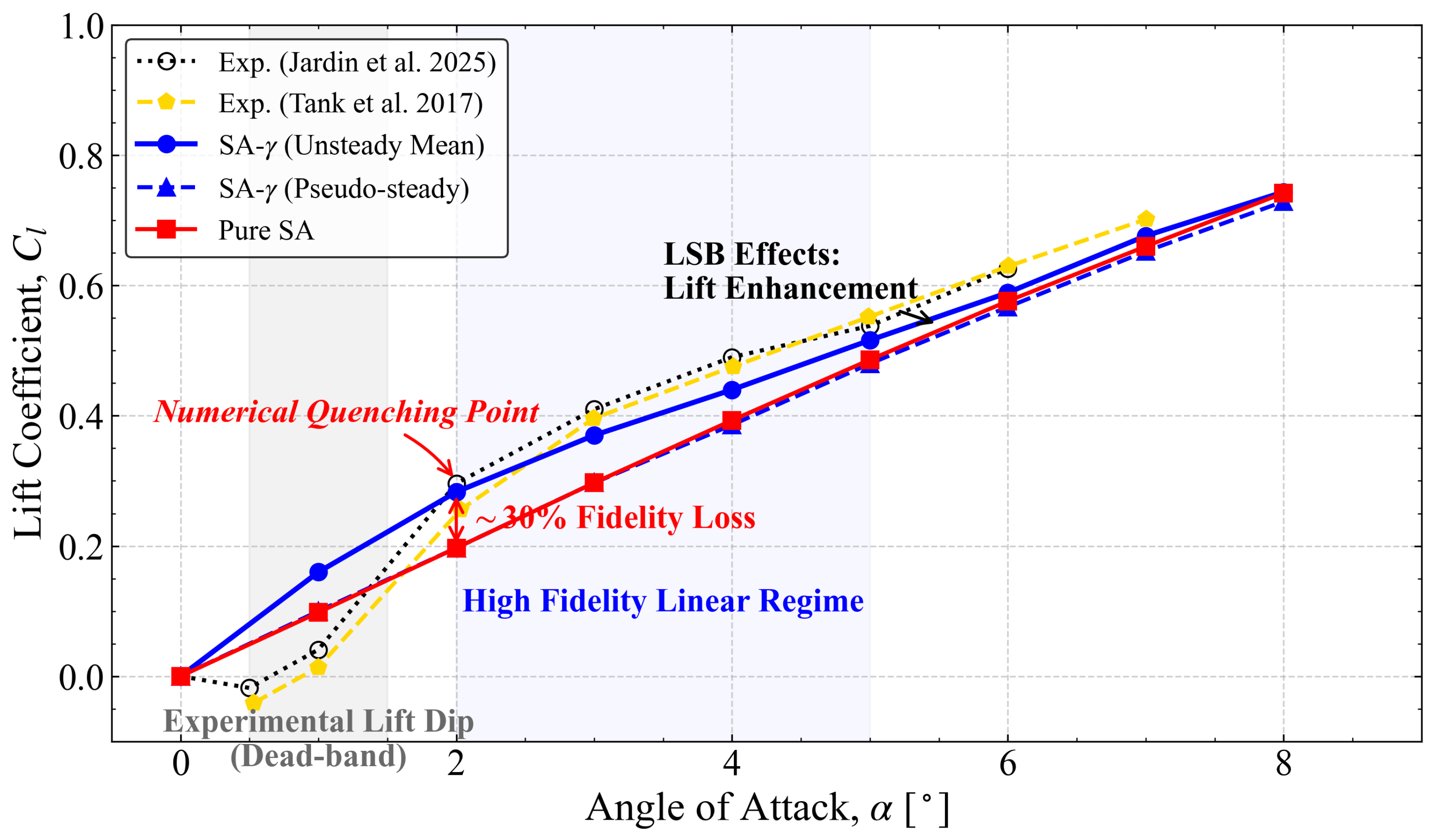
The global aerodynamic coefficients predicted by the SA- model are validated against the high-fidelity experimental datasets of Jardin et al. and Tank et al. Figure 4 presents the lift coefficient () as a function of the angle of attack (). Within the linear regime (), the SA- (Unsteady Mean) results exhibit close agreement with the experimental data, capturing the high lift-curve slope induced by the LSB. In contrast, the fully turbulent Pure SA model underestimates the lift, as it fails to account for the “virtual camber” effect provided by the closed separation bubble [13,14,55].
Figure 4.
Lift coefficient () vs. angle of attack (): Comparison showing the LSB-induced lift enhancement. The “Numerical Quenching Point” at marks the collapse of the physical attractor.
A critical finding in Figure 4 is the identification of a “Numerical Quenching Point” at . At this incidence, the unsteady formulation maintains the physical LSB, whereas the pseudo-steady state suffers a catastrophic bifurcation, leading to a ∼30% lift deficit. This collapse indicates that the transition model regresses to a fully turbulent-like state once the physical instabilities are suppressed by numerical dissipation, revealing a sharp sensitivity of the low- linear regime to numerical dissipation.
3.2.2. Drag Characteristics and the Mechanism of Inversion
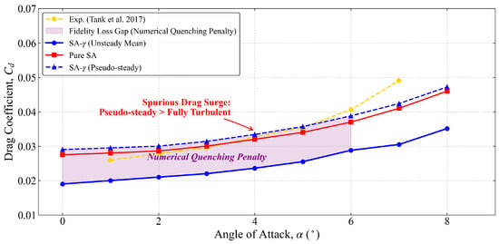
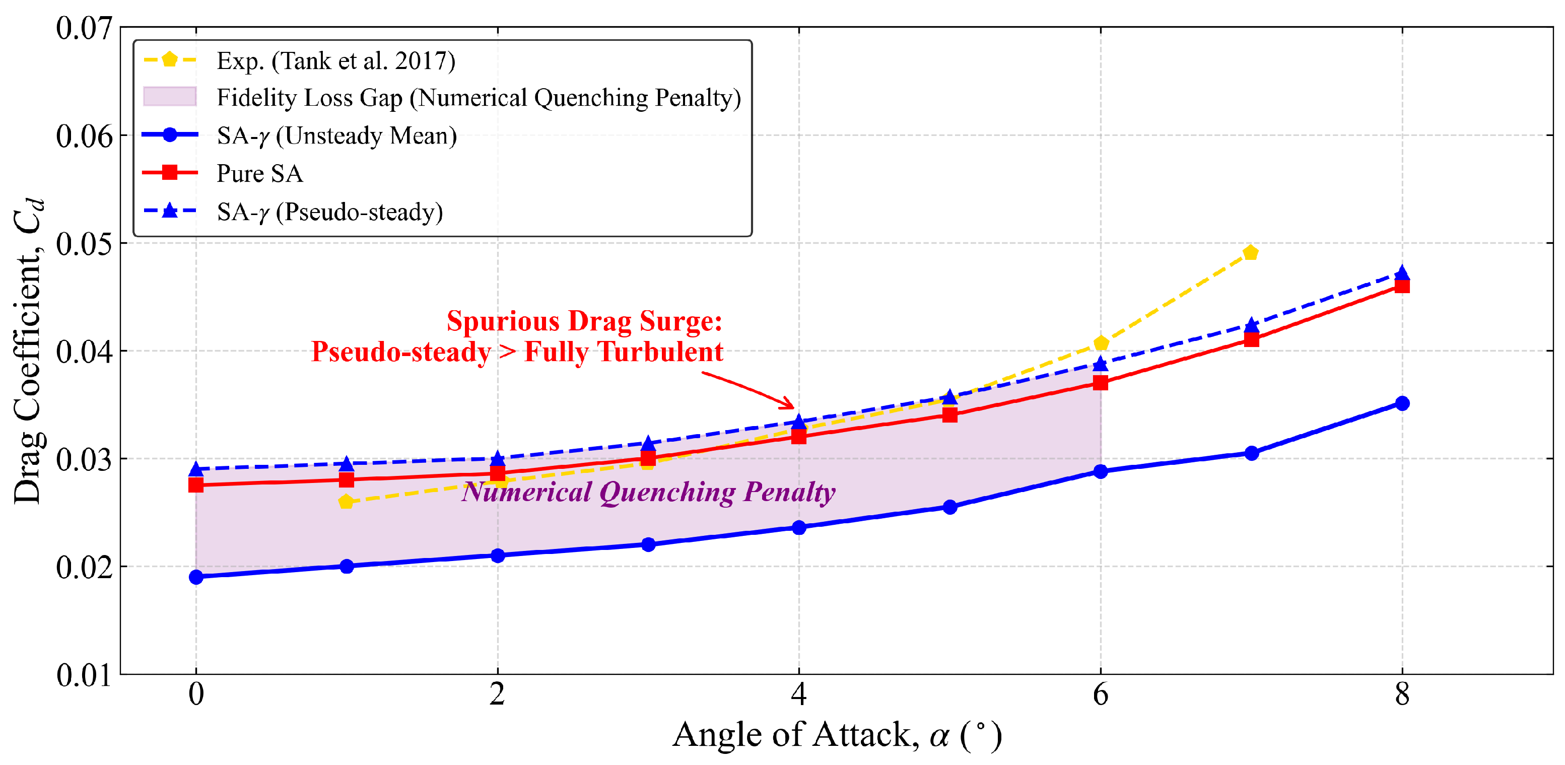
The drag characteristics, illustrated in Figure 5, reveal a counter-intuitive phenomenon termed “Drag Mechanism Inversion”. In conventional aerodynamics, transition modeling is expected to reduce drag by preserving laminar flow. However, for , the SA- (Unsteady) model aligns closely with the experimental measurements of Tank et al. [23]. This suggests that the LSB-induced pressure drag is the dominant resistance mechanism in this regime. This inversion is further supported by an analysis of the boundary layer shape factor , which remains high (∼3.5) within the separation zone, indicating a significant energy deficit that precludes the recovery of suction-side pressure.
Figure 5.
Drag coefficient () vs. angle of attack (): Evidence of the “Drag Mechanism Inversion” where numerical quenching leads to a spurious drag surge exceeding turbulent levels.
More importantly, Figure 5 quantifies the “Numerical Quenching Penalty” (shaded region). When the LSB dynamics collapse into a pseudo-steady state, the drag does not merely increase—it surges to a level that exceeds even the fully turbulent Pure SA baseline. This spurious drag surge is a direct consequence of numerical dissipation inducing a non-physical, over-extended separation topology.
The comparison in Figure 5 highlights that fully turbulent baselines can under-represent LSB-induced form drag at these conditions. More broadly, it reinforces that residual convergence alone does not identify the physically relevant branch in transitional separated flows; the correct dynamical state must be diagnosed via phase-space and spectral signatures.
3.2.3. Aerodynamic Polar and Efficiency Analysis
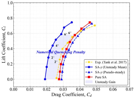
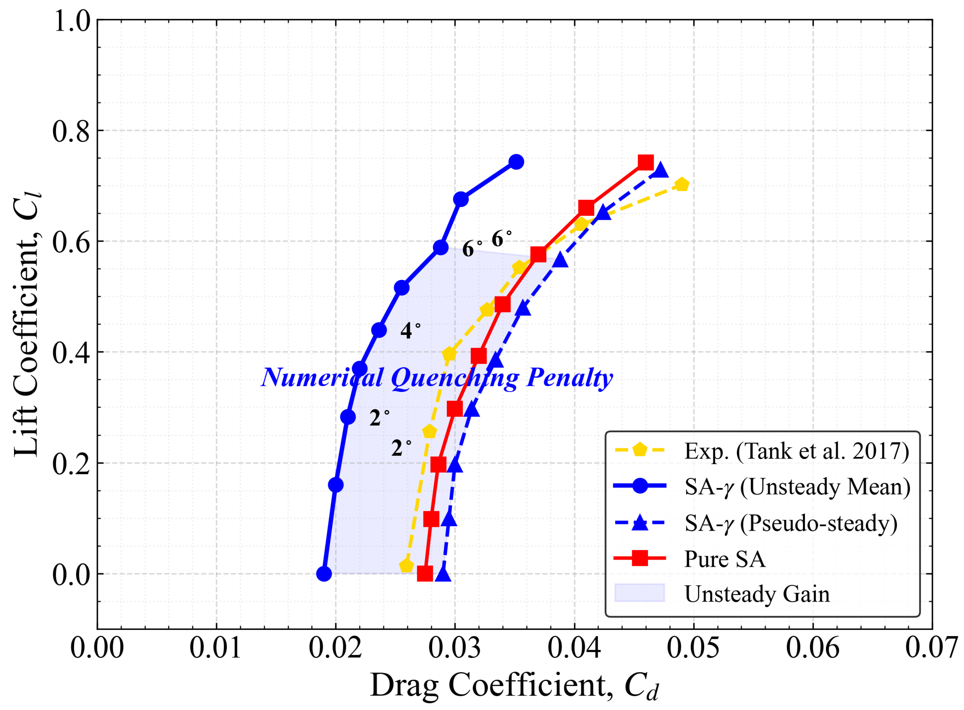
The integrated impact of these numerical artifacts is summarized in the aerodynamic drag polar (Figure 6). The “Unsteady Gain” shaded region in the polar plot represents the significant aerodynamic envelope recovered by resolving the dynamic LSB. This gain is not merely a quantitative increment but a qualitative expansion of the flight envelope. The phase-space separation between the unsteady attractor and the pseudo-steady fixed point confirms the Stability–Fidelity Paradox: the pursuit of a stable, converged solution leads to a fixed-point attractor that resides far from the physical reality, effectively shrinking the operational domain of the airfoil.
Figure 6.
Aerodynamic drag polar ( vs. ): Visualization of the topological separation between the physical limit-cycle attractor and the pseudo-steady attractor.
3.2.4. Aerodynamic Efficiency and Integrated Effects
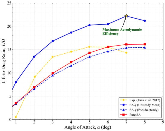
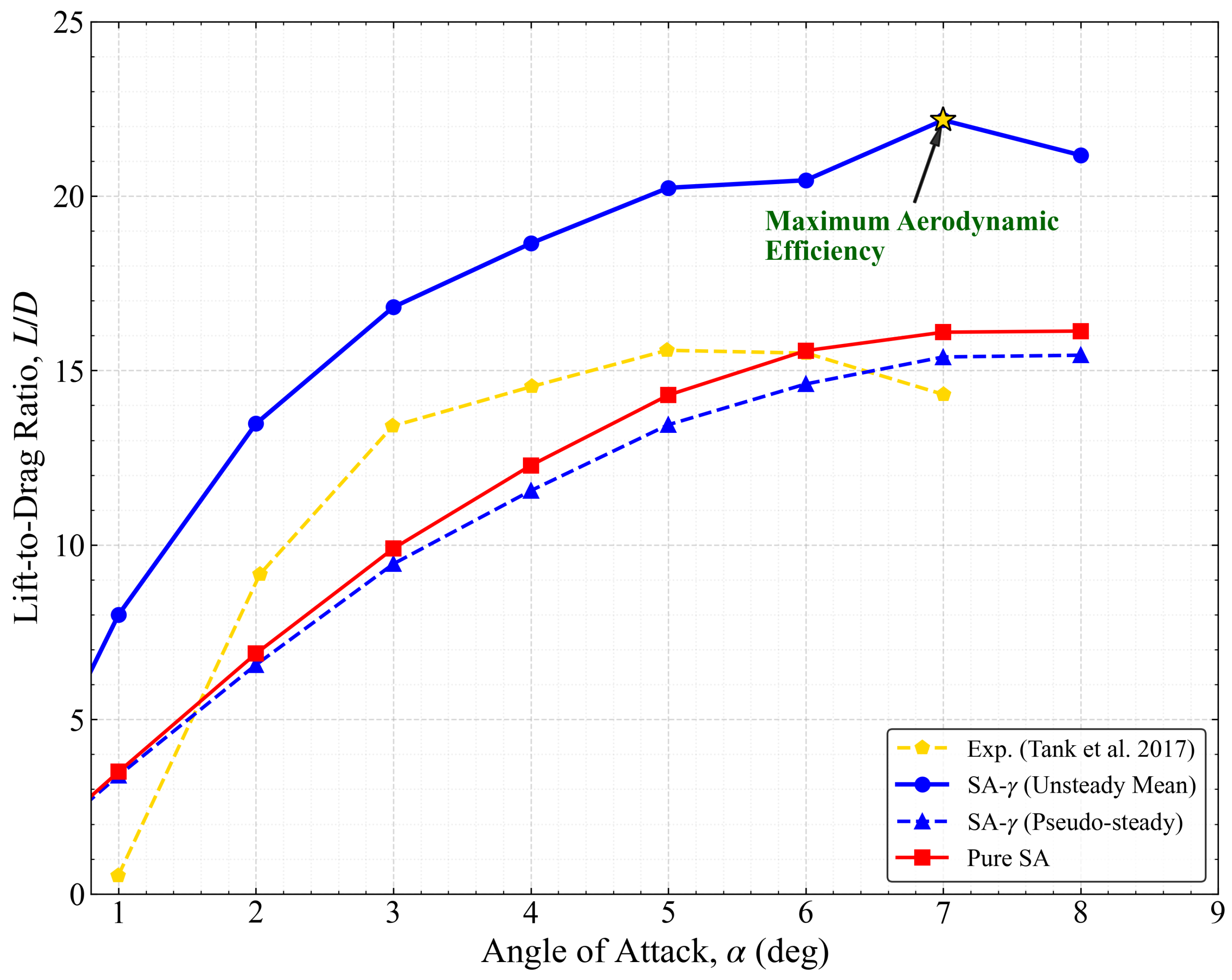
The integrated impact of numerical quenching is evident in the lift-to-drag ratio. The SA- (Unsteady Mean) model identifies a peak aerodynamic efficiency of at , before declining to at (Figure 7). This delayed peak, compared to typical experimental stall around , is attributed to the 2D assumption which precludes the formation of 3D stall cells, thereby artificially extending the linear lift regime. In stark contrast, both the Pure SA and the pseudo-steady SA- results exhibit a systematic underprediction of efficiency across the linear range. Conversely, at higher incidences (), while the fully turbulent Pure SA model continues to underpredict the absolute efficiency due to excessive skin friction, it qualitatively fails to capture the physical onset of separation, exhibiting a monotonic behavior in that misses the characteristic efficiency drop observed in the unsteady transitional physics. Specifically, at , the pseudo-steady state predicts an of only 14.5—a 30% efficiency deficit compared to the unsteady-mean result. For low-Reynolds-number aerial vehicles, such as the Mars Helicopter, this deficit translates directly into a 30% reduction in estimated range and endurance, highlighting the critical engineering risk of relying on quenched RANS solutions.
Figure 7.
Lift-to-drag ratio () comparison: Identification of peak efficiency and the deficit induced by numerical quenching.
3.3. Numerical Dynamics and the Stability–Fidelity Paradox
The previous sections established that the SA- model can achieve high predictive fidelity, but only when the unsteady nature of the LSB is fully resolved. However, a critical “Stability–Fidelity Paradox” emerges when considering the long-term temporal evolution of the solution. This paradox posits that the pursuit of numerical stability—manifested as converged steady-state residuals—often leads to the artificial suppression of physical instabilities, a process we term “Numerical Quenching.”
In the following analyses, we define the pseudo-steady state strictly by two objective signatures: (i) the collapse of the phase-space limit cycle to a fixed-point attractor in the - plane (Figure 11), and (ii) the disappearance of the characteristic dominant Strouhal peak in the lift fluctuation spectrum (Figure 10). This definition is intentionally independent of residual convergence, as residual-based criteria are shown to be misleading in this transitional regime.
3.3.1. The Pseudo-Convergence Trap at Low Incidence ()
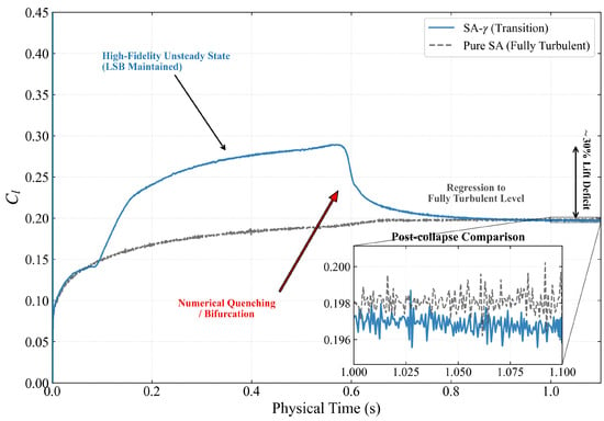
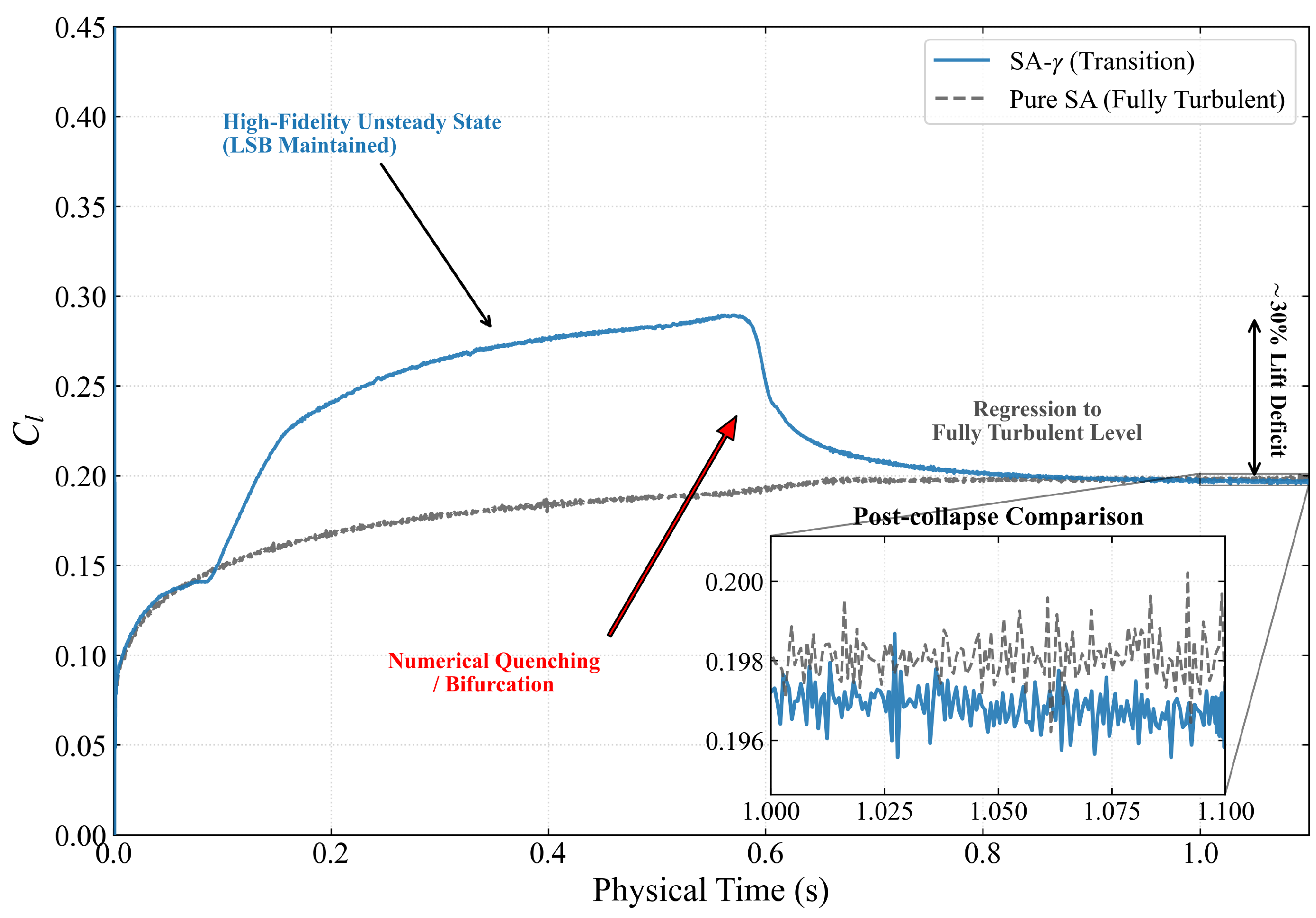
At low angles of attack, the LSB is relatively thin and sensitive to numerical dissipation. Figure 8 illustrates the time-history of the lift coefficient at . Initially, the SA- model resolves a high-fidelity unsteady state (), which aligns closely with the experimental benchmark. In this phase, the model successfully maintains the LSB structure and its associated lift enhancement.
Figure 8.
Time-history of lift coefficient at (Time step s, Inner iterations = 20): Demonstration of the “pseudo-convergence trap” where the transition model regresses to the fully turbulent baseline level. The physical time step is s, meaning s corresponds to 5000 iterations.
However, at s, the solution undergoes a sudden numerical bifurcation. The physical fluctuations are quenched by the cumulative effect of numerical dissipation, and the lift coefficient suffers a catastrophic collapse. The delayed onset of quenching at s suggests that the numerical dissipation acts as a slow-acting damping force, gradually eroding the limit-cycle energy until the trajectory crosses a separatrix into the basin of attraction of the fixed-point solution. It is emphasized that this pseudo-steady state is not the result of a steady-state solver but is obtained via the same time-accurate integration where the solution naturally settles into a fixed point (damped oscillation), as shown in Figure 8. As shown in the inset of Figure 8, the post-collapse state (pseudo-steady) exhibits a perfect numerical overlap with the Pure SA (fully turbulent) baseline (). This “topological regression” indicates that the transition model has effectively undergone a spurious collapse in which the solver’s drive toward a fixed-point attractor overrides the nonlinear source terms required to sustain the LSB. This demonstrates that well-converged residuals can coexist with large biases in the integrated loads when the dynamical state is misidentified.
3.3.2. Bifurcation and Spurious Drag Surge at High Incidence ()
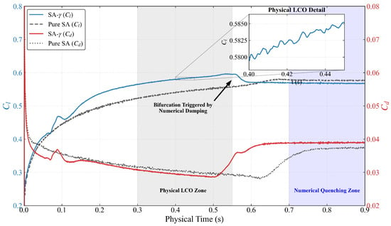
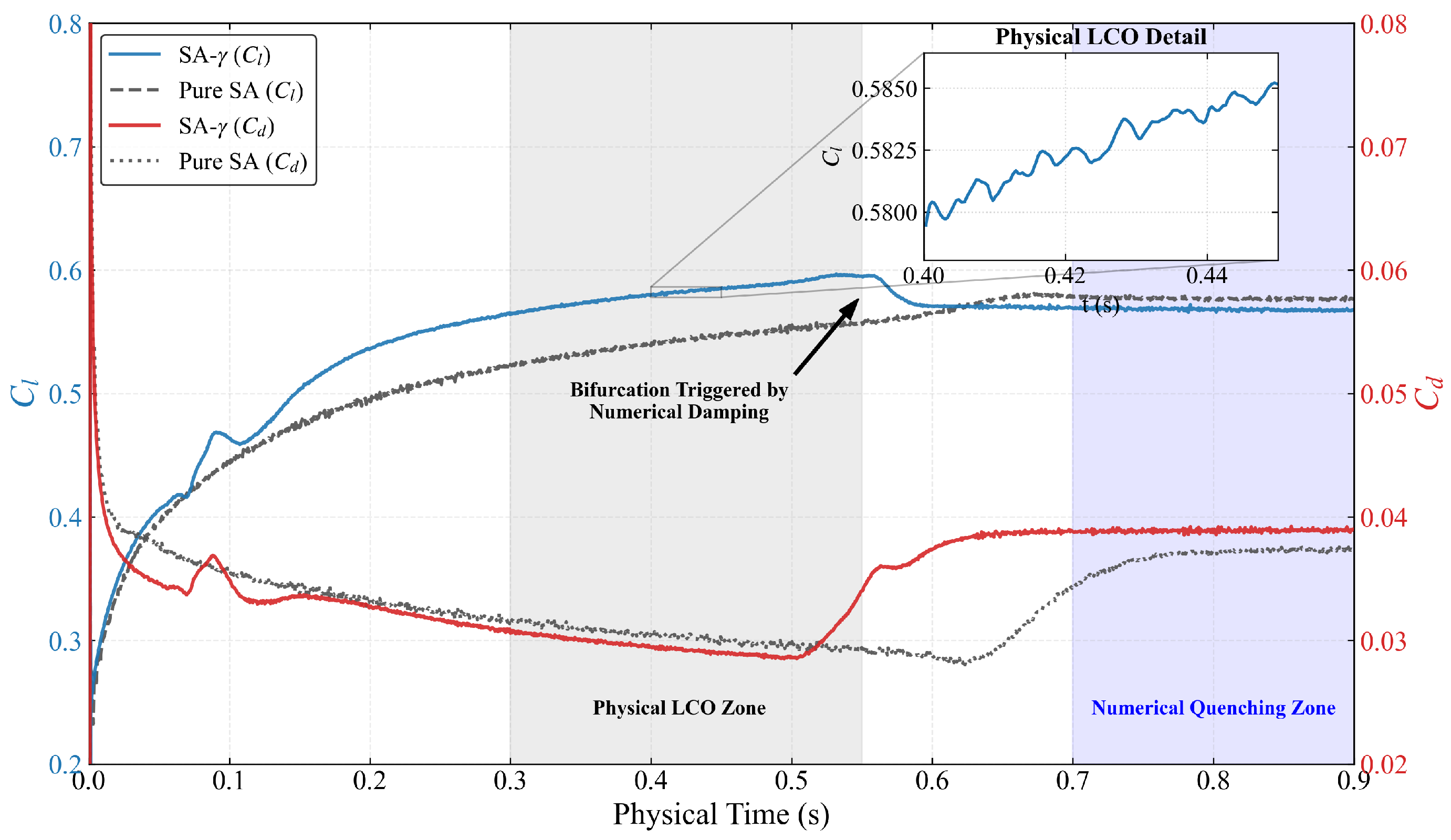
The paradox becomes even more pronounced as the flow approaches the stability boundary. Figure 9 presents the dual-axis time-history of and at . In the “Physical LCO Zone” (), the model resolves robust LCO. High-resolution inset confirms that these are not numerical noise but coherent physical pulsations associated with periodic vortex shedding from the LSB.
Figure 9.
Dual-axis time-history of and at (Time step s, Inner iterations = 20): Visualization of the transition from physical LCO to numerical quenching. The simultaneous lift collapse and drag surge highlights the catastrophic failure of the pseudo-steady attractor. The physical time step is s, meaning s corresponds to 5000 iterations.
The transition to the “Numerical Quenching Zone” after s reveals the penalty of pseudo-convergence. As the oscillations are damped out, the flow does not merely settle into the mean of the LCO; instead, it transitions to a branch characterized by a simultaneous drop in lift and a surge in drag. Specifically, at s, the drag coefficient reaches , consistent with the total height of the pseudo-steady column in the drag decomposition analysis (Section 3.4.4). The duration of this drag surge (from s to s) corresponds to approximately 2–3 convective timescales, aligning with the dominant shedding period of the LSB shear layer (). This confirms that the step-change is a direct physical manifestation of the separation bubble bursting and the subsequent irreversible widening of the wake, rather than an algorithmic instability.
To rigorously verify whether the “numerical quenching” is merely an artifact of the 2nd-order upwind scheme’s diffusion, we conducted an additional simulation at the critical angle of using the higher-order, low-dissipation MUSCL 3rd-order scheme for the convection terms. Crucially, the MUSCL 3rd-order scheme inevitably leads to the identical numerical quenching, collapsing to a pseudo-steady state with nearly identical coefficients (). This proves that the bifurcation is not a trivial discretization error caused by the upwind scheme, but a robust topological property of the URANS framework itself where the modeling dissipation of the SA- closure acts as a low-pass filter.
This bifurcation at is not merely a numerical artifact but a manifestation of the “Stability-Fidelity Paradox.” The RANS operator, when over-damped, acts as a spectral filter that dissipates the energy of Kelvin–Helmholtz instabilities required to sustain LSB breathing. Consequently, the flow collapses from a limit-cycle attractor (the physical state) to a fixed-point attractor (the numerical state). This implies that a converged steady-state solution in this regime can be physically incorrect.
3.3.3. Spectral Characteristics of Unsteady Fluctuations
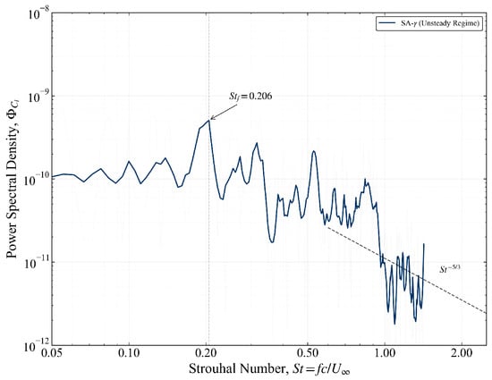
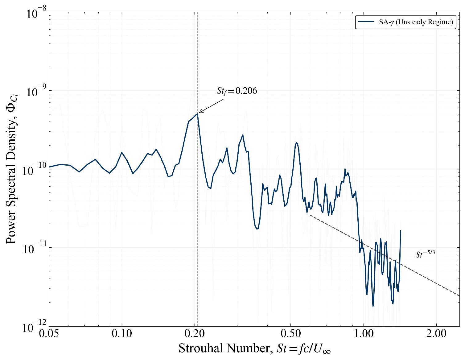
To verify that the captured lift fluctuations are driven by coherent physical mechanisms rather than numerical noise, a spectral analysis of the time-history at is performed. Figure 10 presents the PSD as a function of the Strouhal number (). The spectral analysis was performed over a sampling window of with a sampling frequency corresponding to the physical time step ( s). A Hanning window was applied to minimize spectral leakage. The spectrum reveals a sharp, dominant tonal peak at , which corresponds to the fundamental frequency of the physical LCO.
Figure 10.
PSD of lift fluctuations at : The dominant peak at is consistent with shear-layer shedding reported in the experimental benchmarks of Yarusevych et al. [18]. The spectrum also exhibits broadband high-frequency content prior to numerical quenching.
This frequency is consistent with characteristic vortex shedding frequencies reported in the experimental studies of Yarusevych et al. [18] and the recent benchmarks of Jardin et al. [22] for airfoils at transitional Reynolds numbers. The presence of this distinct peak indicates that the SA- model, when coupled with a high-resolution temporal scheme ( s), captures the dominant Kelvin-Helmholtz (K-H) instability within the separated shear layer prior to numerical quenching.
3.3.4. Dynamical System Analysis: Phase Portraits and Attractors
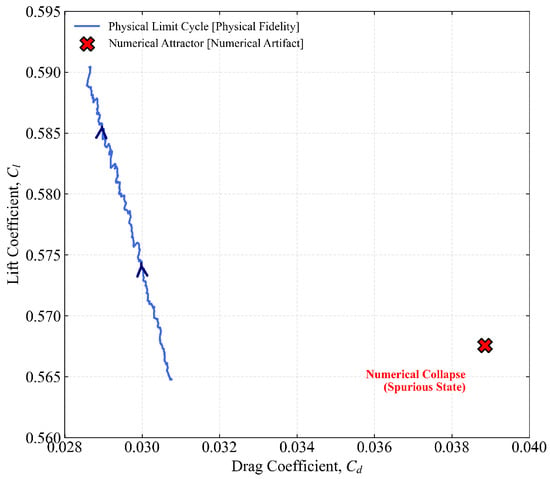
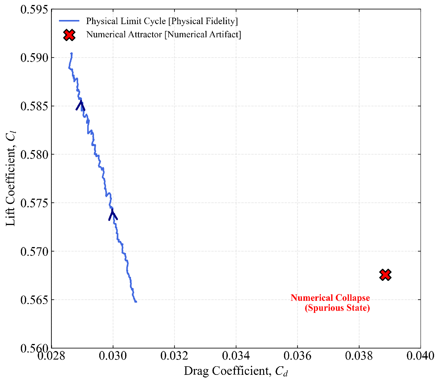
The dynamical nature of this bifurcation is further quantified via the phase portrait in the - plane (Figure 11). The phase portrait reveals the topological essence of the flow. The physical solution manifests as a robust limit-cycle attractor, representing the continuous intake and exhaust of energy driven by LSB vortex shedding. In contrast, the pseudo-steady state is identified as a spurious fixed-point attractor, where the system’s energy is entirely dissipated by numerical dissipation. The distinct separation in phase space indicates a topological change in the solution, not just a quantitative error.
Figure 11.
Phase portrait in the - plane at : Geometric separation between the physical limit-cycle attractor and the spurious fixed-point attractor.
This transition suggests that numerical dissipation acts as a hidden bifurcation parameter, forcing the dynamical system to undergo an inverse process of a Hopf Bifurcation. The geometric separation between the limit-cycle and the fixed-point provides a rigorous visual metric for fidelity loss, confirming that numerical quenching induces a fundamental topological shift rather than a simple statistical attenuation.
3.4. Microscopic Flow Physics and Quenching Mechanisms
3.4.1. Topological Evolution of the Laminar Separation Bubble
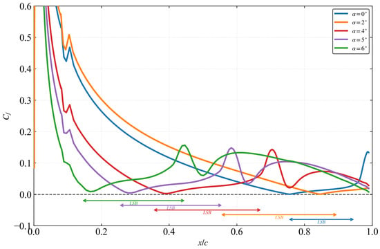
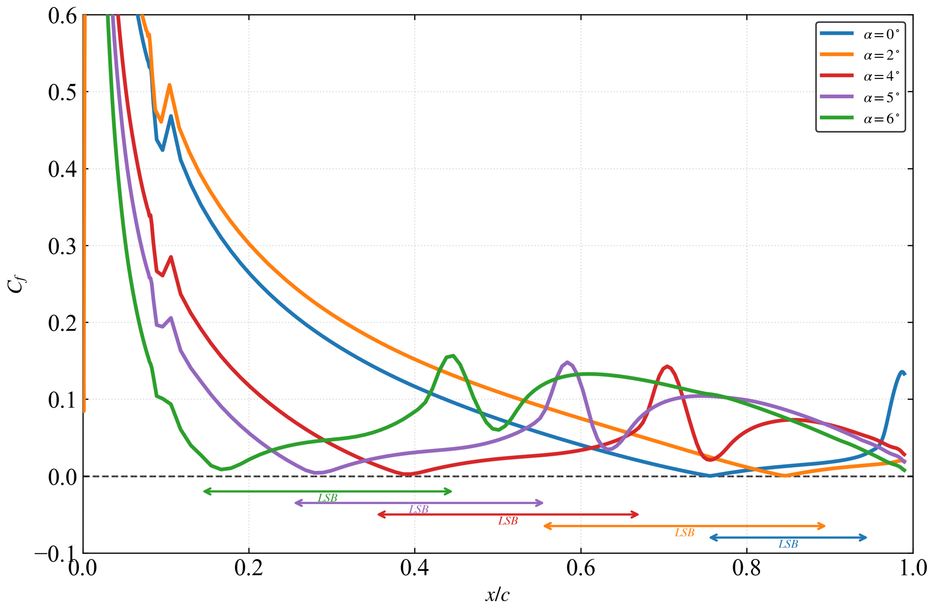
The macroscopic aerodynamic performance is intrinsically linked to the microscopic topology of the LSB. Figure 12 illustrates the chordwise distribution of the time-averaged skin friction coefficient () across the investigated angles of attack (). The extent of the LSB is rigorously identified by the regions of negative skin friction (), highlighted by the colored shading.
Figure 12.
Chordwise distribution of the time-averaged skin friction coefficient () identifying the LSB extent (). The topological contraction of the bubble with increasing is a critical physical feature that is lost during numerical quenching.
As increases, the flow exhibits a characteristic upstream migration and spatial contraction of the bubble. At , the LSB resides near the trailing edge (x/c ≈ 0.75–0.95). As incidence rises to , the separation point () shifts rapidly toward the leading edge (), while the bubble length significantly decreases. This topological evolution is critical; the numerical quenching phenomenon identified in this work is effectively a topological regression, where the solver artificially restores a turbulent-like attached flow topology, erasing the rich LSB structure shown in Figure 12.
Notably, the sharp recovery and overshoot of immediately downstream of the shaded regions (e.g., at for ) confirm the transition to a fully developed turbulent boundary layer. This topological capture validates that the unsteady SA- model correctly resolves the recirculation core and the subsequent turbulent re-energization, distinguishing it from the “quenched” solutions discussed in Section 3.2.
3.4.2. Surface Physics and the “Self-Quenching” Mechanism
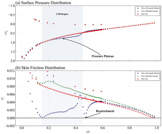
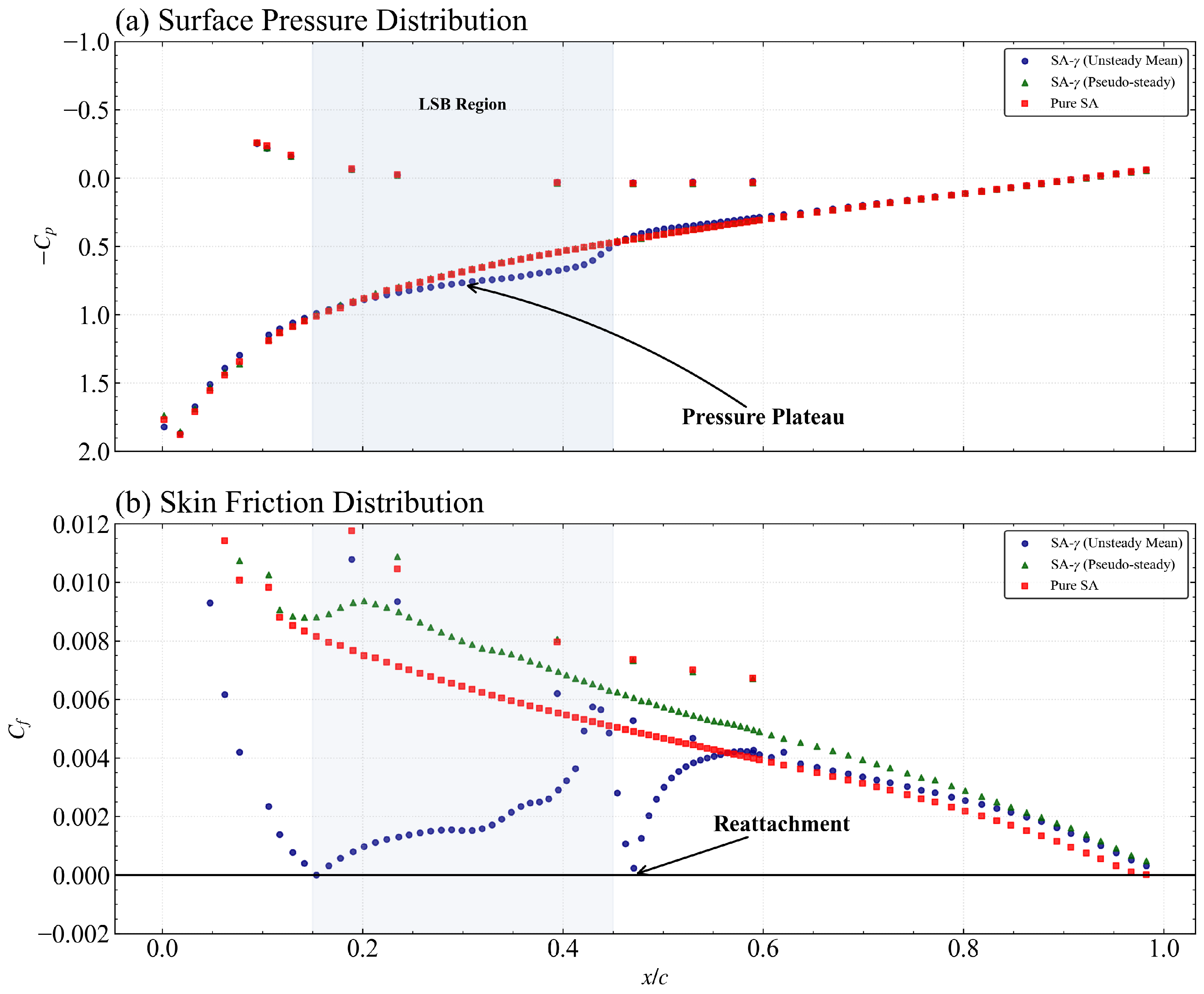
To elucidate the microscopic origin of the fidelity loss identified in the global coefficients, the surface pressure coefficient () and skin friction coefficient () distributions at are analyzed in Figure 13. Unlike previous studies that relied solely on pressure coefficients [30,37], we explicitly analyze the skin friction topology to pinpoint the separation () and reattachment () points with high precision. The SA- (Unsteady Mean) model resolves a distinct pressure plateau on the suction surface between and (Figure 13a), which is the classic aerodynamic signature of a closed LSB [13]. This is further confirmed by the distribution (Figure 13b), where the unsteady-mean results exhibit a negative friction zone, precisely identifying the recirculation core of the bubble.
Figure 13.
Surface aerodynamic distributions at . (a) Pressure coefficient (); (b) Skin friction coefficient (). Only the suction surface distributions are shown for clarity. The disappearance of the suction-side pressure plateau confirms the topological regression to a turbulent-like flow.
A striking observation in Figure 13 is the near-overlap between the SA- (Pseudo-steady) and the Pure SA distributions. This provides strong evidence of the numerical quenching phenomenon: once the physical instabilities are suppressed by numerical dissipation, the transition model fails to maintain the laminar portion of the separation bubble. The flow topology regresses toward a fully turbulent-like state, where the pressure plateau vanishes and the separation signature is substantially weakened. This topological regression—characterized by the disappearance of the negative zone—accounts for the ∼30% lift deficit observed in the pseudo-steady regime.
3.4.3. Boundary Layer Energetics and Velocity Profiles
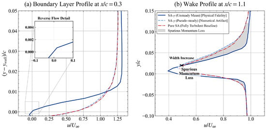
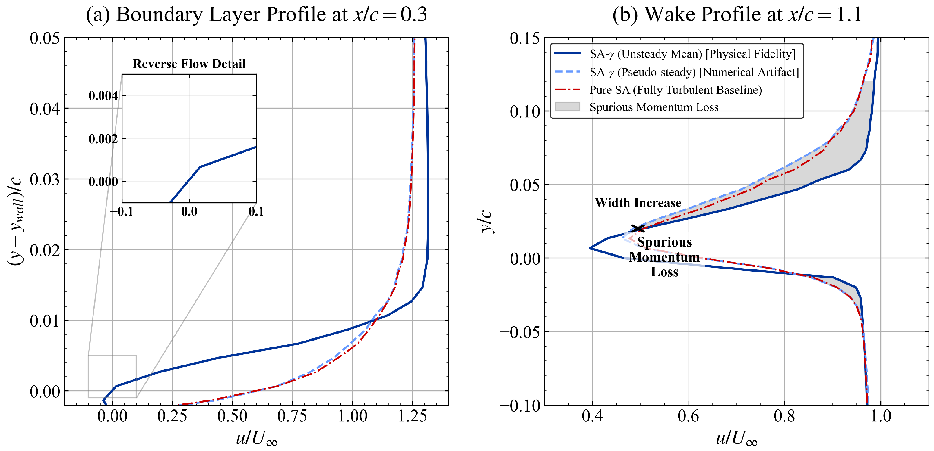
The impact of numerical quenching on the boundary layer structure and wake energetics is visualized through the velocity profiles in Figure 14. At the LSB core (, Figure 14a), the unsteady-mean profile resolves a robust reverse-flow region (see the “Reverse Flow Detail” inset), which is essential for preserving the physical displacement effect of the bubble. In contrast, the pseudo-steady and Pure SA profiles exhibit a stagnant, “sluggish” boundary layer without the characteristic flow reversal, indicating a failure to resolve the LSB internal dynamics.
Figure 14.
Velocity profiles at comparing unsteady-mean and pseudo-steady states. The “Spurious Momentum Loss” in the wake (b) provides a kinematic explanation for the drag inversion, linking wake broadening to entropy generation.
The clearest signature of the drag surge is found in the near-wake profile at (Figure 14b). The pseudo-steady state produces a substantially wider and deeper velocity deficit compared to the unsteady-mean result. The shaded area, termed the “Spurious Momentum Loss,” provides a kinematic visualization of the drag penalty identified in Section 3.2.2. According to the momentum integral theorem, this expanded deficit implies an increase in momentum thickness, consistent with the observed pressure drag surge [56]. These results indicate that the drag increase is associated with an altered wake topology (i.e., wake broadening). This provides a direct link between the microscopic failure of the transition model (quenching of K-H instability) and the macroscopic drag penalty, confirming that the drag inversion is physically rooted in wake thermodynamics rather than numerical error alone. The pseudo-steady state induces a highly dissipative, over-extended wake topology that represents a particularly adverse outcome for low- simulations.
3.4.4. Drag Decomposition and Pressure-Viscous Partitioning
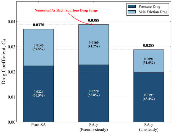
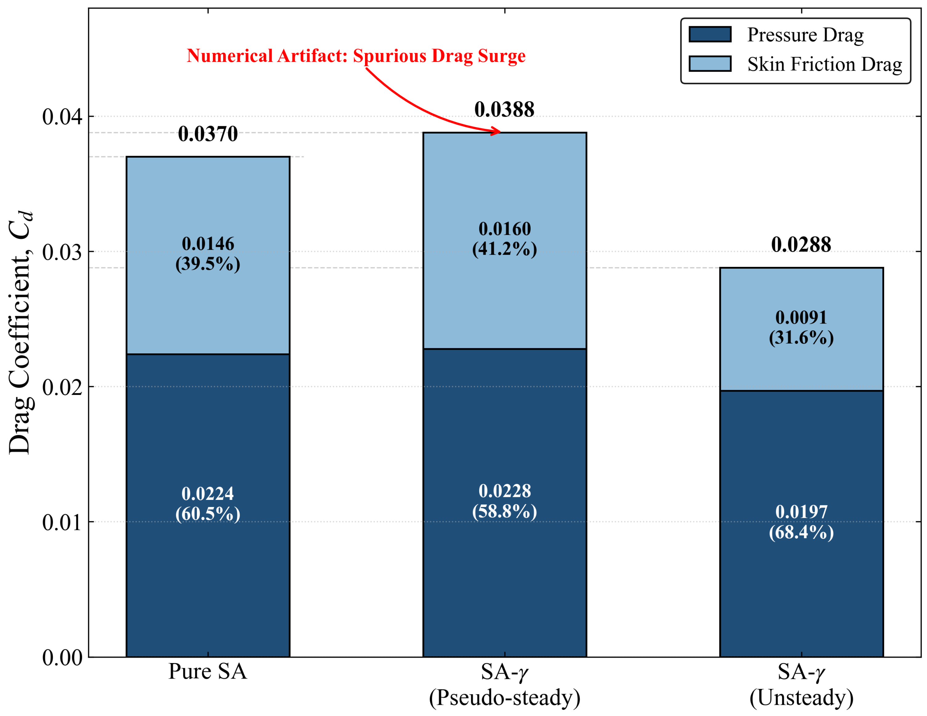
To further isolate the influence of numerical quenching on aerodynamic resistance, a quantitative decomposition of the total drag coefficient () into pressure drag () and skin friction drag () is performed at (Figure 15). The results reveal a striking “Drag Mechanism Inversion” triggered by the stability–fidelity paradox.
Figure 15.
Quantitative drag component decomposition at : Stacked bar chart illustrating the surge in pressure drag induced by numerical quenching.
As illustrated in Figure 15, the SA- (Unsteady Mean) model yields the lowest total drag (), where the skin friction component accounts for only 31.6% of the total resistance. This confirms the “laminar benefit” recovered by the transition model when physical instabilities are resolved. However, upon collapsing into the pseudo-steady state, the total drag surges to , a value that surprisingly exceeds the Pure SA baseline (). From a thermodynamic perspective, this spurious drag surge is associated with the enhanced entropy generation within the artificially thickened wake; the suppression of discrete vortices leads to a highly dissipative shear-layer topology that increases irreversible losses.
This spurious drag surge is driven by a dual-failure mechanism: (1) a 75% increase in skin friction ( to ) as the laminar portion of the bubble is prematurely turbulentized; and (2) a non-physical rise in pressure drag ( to ). The fact that the pseudo-steady transition model predicts a higher pressure drag than the fully turbulent model—which assumes a fully attached flow—indicates that numerical dissipation induces a “frozen,” over-extended separation topology.
The inversion of the drag mechanism at illustrates that suppressing the unsteady LSB dynamics can shift the balance between viscous and form drag. The pseudo-steady branch yields a drag level that exceeds the fully turbulent baseline, consistent with an over-extended separation and a broadened wake. This behavior emphasizes that, in transitional separated flows, the physical interpretation of drag levels must be tied to the resolved dynamical state and wake topology rather than residual-based convergence alone. From a thermodynamic perspective, the pseudo-steady branch corresponds to a more dissipative wake with increased irreversible entropy production, consistent with the observed momentum deficit and drag surge.
3.4.5. Coherent Flow Structures and Vortical Decay
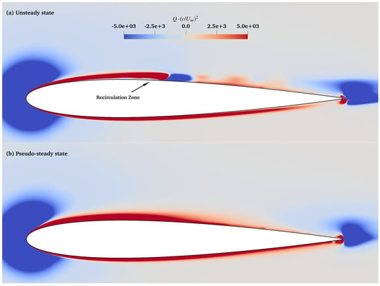
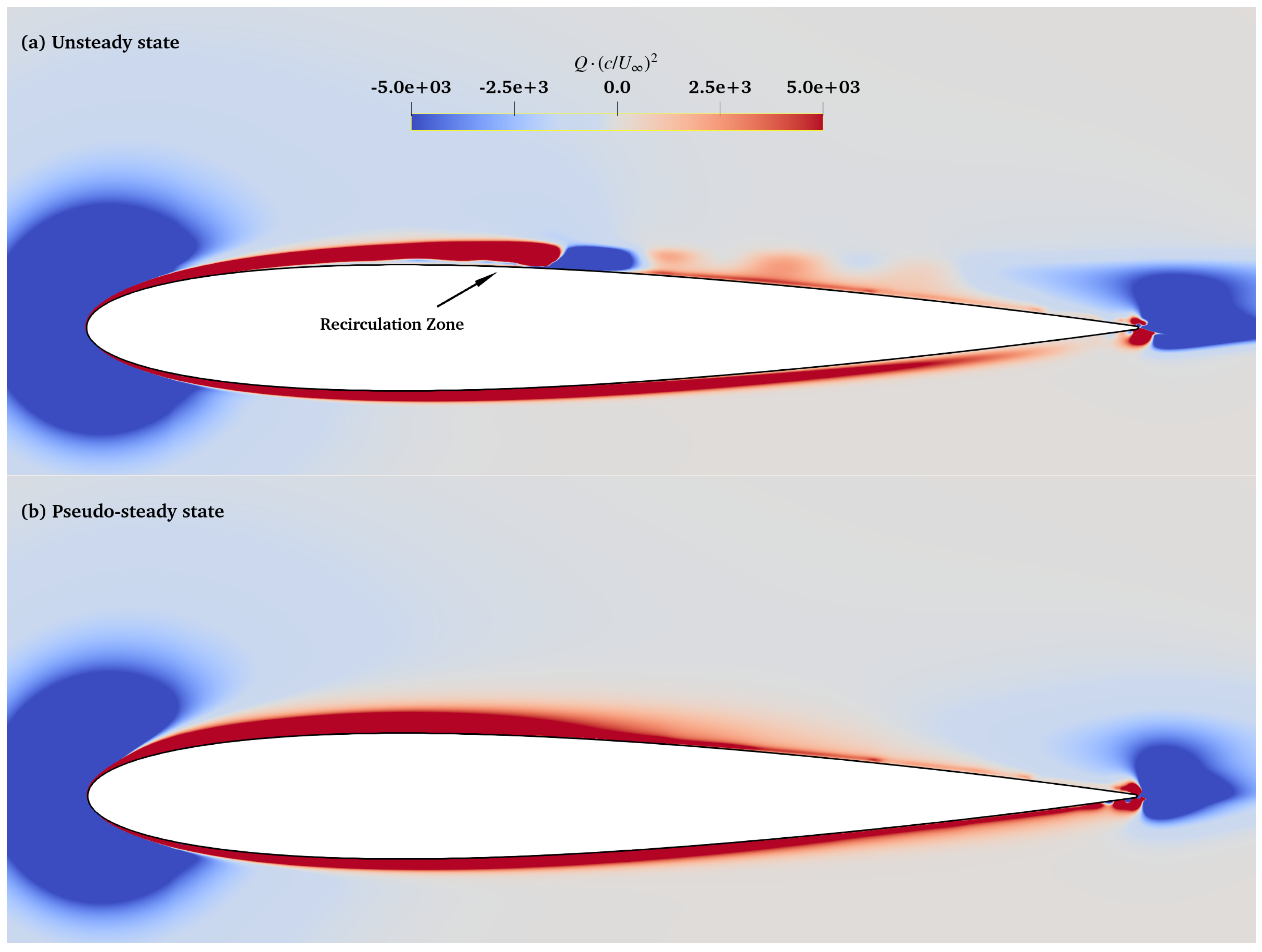
The topological shift responsible for the performance collapse is visually confirmed through the instantaneous Q-criterion distributions in Figure 16. In the unsteady state (Figure 16a), the SA- model resolves the periodic roll-up and shedding of discrete vortical structures from the LSB shear layer [17,40]. A well-defined recirculation zone is encapsulated beneath the separated shear layer, which maintains the physical pressure distribution and high lift fidelity. These coherent structures enhance vertical momentum exchange, effectively “energizing” the wake.
Figure 16.
Instantaneous vortical structures visualized by the Q-criterion (). (a) The physical attractor resolves coherent vortex shedding. (b) The pseudo-steady attractor exhibits numerical silence, visually confirming the suppression of the Kelvin-Helmholtz instability by numerical dissipation.
In stark contrast, the pseudo-steady state (Figure 16b) exhibits numerical silence. The discrete vortices are suppressed, and the shear layer is smeared into a continuous, diffused band of high vorticity. This visualization supports the numerical quenching interpretation: the solver’s numerical dissipation acts as a low-pass filter that attenuates the non-linear energy of the K-H instabilities [43]. The resulting separation bubble fails to re-energize the boundary layer, leading to a thickened wake and the momentum loss previously quantified in Figure 14.
This numerical silence is not merely a visual difference but represents a fundamental failure to capture the energetic breathing of the separation bubble, effectively creating a barrier to high-fidelity prediction in the low-Reynolds-number regime. Together with the spectral and quantitative analyses, this supports the conclusion that residual convergence in this regime can be a misleading indicator of physical correctness.
4. Conclusions
This study investigates the boundary of predictive fidelity for the SA- transition model on a NACA 0012 airfoil at . By diagnosing the topological evolution of the Laminar Separation Bubble (LSB) and conducting dynamical system analyses, the following conclusions are drawn:
- Numerical Quenching as a System Bifurcation: The pursuit of residual convergence in URANS can suppress fundamental physical instabilities. When numerical dissipation overwhelms the K-H amplification, the LSB topology prematurely collapses from a dynamic limit-cycle to a spurious fixed-point attractor. This “quenching” abruptly diminishes the suction-side pressure plateau (), translating to a critical ∼30% deficit in .
- Drag Mechanism Inversion: At the stability boundary (), resolving the physical unsteady LSB confirms that form drag constitutes the majority of the total aerodynamic resistance. However, numerical quenching forces the flow into an over-extended, pseudo-steady separation topology. This artificial state over-predicts momentum thickness, causing the total drag coefficient () to surge past even the pure Spalart-Allmaras (fully turbulent) baseline—an inversion fundamentally rooted in irreversible wake entropy generation.
- The 2D Predictive Boundary and EFD Divergence: While the 2D URANS framework is highly cost-effective in the linear regime (), it inherently lacks the 3D spanwise relief mechanisms present in the Jardin (2025) experiments. Consequently, the modeled 2D vortices maintain absolute coherence, leading to slightly optimistic lift predictions prior to quenching. The model strictly distorts when the physical separation point () migrates forward to and the localized transition mechanisms become highly sensitive to spatial resolution.
- Objective Diagnostics Criteria: Standard CFD best practices are insufficient for low- transitional flows. Analysts must rely on phase-space trajectories (e.g., attractors) and spectral signatures (maintaining ) rather than monotonic residual drops to verify the physical validity of the computed state.
Limitations and Generality: The present conclusions are drawn from a controlled 2D study of the NACA 0012 airfoil at under the specific numerical settings documented herein. While quantitative thresholds will vary with airfoil geometry, inflow turbulence intensity, surface roughness, and three-dimensional effects [1,2,15,57], the underlying LSB mechanism (APG-driven laminar separation followed by shear-layer transition and reattachment) is common to low-Re airfoils. The identified pseudo-convergence trap and associated drag bias should therefore be regarded as a general warning mechanism for transitional separated flow simulations when numerical dissipation is comparable to the intrinsic instability growth.
Future investigations will extend this framework to 3D finite wing configurations to explicitly resolve the spanwise instabilities identified as the primary source of the 2D/3D discrepancy at higher angles of attack.
Author Contributions
Conceptualization, G.C.; methodology, H.L. and G.C.; software, H.L.; validation, H.L. and R.Z.; formal analysis, H.L.; investigation, H.L.; resources, G.C.; data curation, H.L.; writing—original draft preparation, H.L.; writing—review and editing, R.Z. and G.C.; visualization, H.L.; supervision, G.C.; project administration, G.C.; funding acquisition, G.C. All authors have read and agreed to the published version of the manuscript.
Funding
Supported by the Start-up Fund for New Talented Researchers from Nanjing Vocational University of Industry Technology (Grant No. YK21-03-04); the Special Fund of the National Key Laboratory of Helicopter Aeromechanics (No. ZAG25006-18).
Institutional Review Board Statement
Not applicable.
Informed Consent Statement
Not applicable.
Data Availability Statement
The data that support the findings of this study are available from the corresponding authors upon reasonable request.
Conflicts of Interest
The authors declare no conflicts of interest.
References
- Mueller, T.J. Low Reynold Number Vehicles; Technical Report AGARD-AG-288; AGARD: Lake Velence, Hungary, 1985. [Google Scholar]
- Lissaman, P.B.S. Low-Reynolds-number Airfoils. Annu. Rev. Fluid Mech. 1983, 15, 223–239. [Google Scholar] [CrossRef] [Scilit]
- Carmichael, B.H. Low Reynolds Number Airfoil Survey; Technical Report NASA CR 165803; NASA: Washington, DC, USA, 1981; Volume 1.
- Ol, M.V.; McAuliffe, B.; Hanff, E.; Scholz, P.; Kaehler, C. Particle image velocimetry measurements of separation bubbles on low Reynolds number airfoils. In Proceedings of the 43rd AIAA Aerospace Sciences Meeting and Exhibit; AIAA: Reston, VA, USA, 2005; p. 5149. [Google Scholar]
- Balaram, B.; Canham, T.; Duncan, C.; Grip, H.F.; Johnson, W.; Maki, J.; Quon, A.; Stern, R.; Zhu, D. Mars Helicopter Technology Demonstrator. In Proceedings of the 2018 AIAA Atmospheric Flight Mechanics Conference, Kissimmee, FL, USA, 8–12 January 2018. [Google Scholar] [CrossRef] [Scilit]
- Johnson, W.; Withrow-Maser, S.; Young, L.; Malpica, C.; Koning, W.J.; Kuang, W.; Fehler, M.; Tuano, A.; Chan, A.; Datta, A. Mars Science Helicopter Conceptual Design; Technical Report; NASA: Washington, DC, USA, 2020.
- Koning, W.J.; Johnson, W.; Allan, B.G. Generation of Mars Helicopter Rotor Model for Comprehensive Analyses; Technical Report; NASA: Washington, DC, USA, 2018.
- Johnson, W. Helicopter Theory; Courier Corporation: Chelmsford, MA, USA, 2012. [Google Scholar]
- Leishman, G.J. Principles of Helicopter Aerodynamics with CD Extra; Cambridge University Press: Cambridge, UK, 2006. [Google Scholar]
- Grip, H.F.; Lam, J.; Bayard, D.S.; Conway, D.T.; Singh, G.; Brockers, R.; Delaune, J.H.; Matthies, L.H.; Malpica, C.; Brown, T.L.; et al. Flight Control System for NASA’s Mars Helicopter. In Proceedings of the AIAA Scitech 2019 Forum, San Diego, CA, USA, 7–11 January 2019. [Google Scholar] [CrossRef] [Scilit]
- Anyoji, M.; Numata, D.; Nagai, H.; Asai, K. Effects of Mach Number and Specific Heat Ratio on Low-Reynolds-Number Airfoil Flows. AIAA J. 2015, 53, 1640–1654. [Google Scholar] [CrossRef] [Scilit]
- Lee, T.; Gerontakos, P. Flow past a NACA 0012 airfoil at low Reynolds numbers. J. Fluid Mech. 2003, 490, 305–316. [Google Scholar] [CrossRef] [Scilit]
- Tani, I. Low-Speed Flows Involving Bubble Separations. Prog. Aerosp. Sci. 1964, 5, 70–103. [Google Scholar] [CrossRef] [Scilit]
- Diwan, S.S.; Ramesh, O.N. Laminar Separation Bubbles: Dynamics and Control. Sadhana 2007, 32, 103–109. [Google Scholar] [CrossRef] [Scilit]
- Gregory, N.; O’reilly, C.L. Low-Speed Aerodynamic Characteristics of NACA 0012 Aerofoil Section, Including the Effects of Upper-Surface Roughness Simulating Hoar Frost; ARC R&M: London, UK, 1970. [Google Scholar]
- Pauley, L.L.; Moin, P.; Reynolds, W.C. The Structure of Two-Dimensional Separation. J. Fluid Mech. 1990, 220, 397–411. [Google Scholar] [CrossRef] [Scilit]
- Sandham, N.D. Flow Separation and Transition; Lecture Series; Von Karman Institute: Sint-Genesius-Rode, Belgium, 2008. [Google Scholar]
- Yarusevych, S.; Sullivan, P.E.; Kawall, J.G. Coherent Structures in an Airfoil Boundary Layer and Wake at Low Reynolds Numbers. Phys. Fluids 2006, 18, 044101. [Google Scholar] [CrossRef] [Scilit]
- O’Meara, T.J.; Mueller, T.J. The laminar separation bubble and its effect on the performance of a low-Reynolds-number airfoil. AIAA J. 1987, 25, 1035–1041. [Google Scholar] [CrossRef] [Scilit]
- Gaster, M. The Structure and Behaviour of Laminar Separation Bubbles; ARC R&M: London, UK, 1967. [Google Scholar]
- Horton, H.P. A Semi-Empirical Theory for the Growth and Bursting of Laminar Separation Bubbles; ARC R&M: London, UK, 1967. [Google Scholar]
- Jardin, T.; Ferrand, V.; Gowree, E.R. NACA0012 Airfoil at Reynolds Numbers between 50,000 and 140,000—Part 1: Steady Freestream. Int. J. Heat Fluid Flow 2025, 112, 109655. [Google Scholar] [CrossRef] [Scilit]
- Tank, J.; Smith, L.; Spedding, G.R. On the Possibility (or Lack Thereof) of Agreement between Experiment and Computation of Flows over Wings at Moderate Reynolds Number. Interface Focus 2017, 7, 20160076. [Google Scholar] [CrossRef] [Scilit]
- Anderson, J. EBOOK: Fundamentals of Aerodynamics (SI Units); McGraw Hill: Columbus, OU, USA, 2011. [Google Scholar]
- Jones, L.E.; Sandberg, R.D.; Sandham, N.D. Direct Numerical Simulations of Forced and Unforced Separation Bubbles on an Airfoil at Incidence. J. Fluid Mech. 2008, 602, 175–207. [Google Scholar] [CrossRef] [Scilit]
- Rist, U.; Maucher, U. Direct Numerical Simulation of 2-D and 3-D Instability Waves in a Laminar Separation Bubble. In Proceedings of the Application of Direct and Large Eddy Simulation to Transition and Turbulence; Cantwell, B., Ed.; AGARD: Lake Velence, Hungary, 1994; pp. 34-1–34-7. [Google Scholar]
- Sagaut, P. Large Eddy Simulation for Incompressible Flows: An Introduction, 3rd ed.; Springer: Berlin/Heidelberg, Germany, 2006. [Google Scholar] [CrossRef] [Scilit]
- Spalart, P.R. Strategies for Turbulence Modelling and Simulations. Int. J. Heat Fluid Flow 2000, 21, 252–263. [Google Scholar] [CrossRef] [Scilit]
- Windte, J.; Scholz, U.; Radespiel, R. Validation of the RANS-simulation of laminar separation bubbles on airfoils. Aerosp. Sci. Technol. 2006, 10, 484–494. [Google Scholar] [CrossRef] [Scilit]
- Catalano, P.; Tognaccini, R. RANS Analysis of the Low-Reynolds Number Flow around the SD7003 Airfoil. Aerosp. Sci. Technol. 2011, 15, 615–626. [Google Scholar] [CrossRef] [Scilit]
- Drela, M. XFOIL: An Analysis and Design System for Low Reynolds Number Airfoils. In Low Reynolds Number Aerodynamics; Brebbia, C.A., Orszag, S.A., Seinfeld, J.H., Spanos, P., Cakmak, A.S., Silvester, P., Desai, C.S., Pinder, G., McCrory, R., Yip, S., et al., Eds.; Springer: Berlin/Heidelberg, Germany, 1989; Volume 54, pp. 1–12. [Google Scholar] [CrossRef] [Scilit]
- Morgado, J.C.P.J.; Vizinho, R.; Silvestre, M.A.R.; Páscoa, J.C. XFOIL vs CFD Performance Predictions for High Lift Low Reynolds Number Airfoils. Aerosp. Sci. Technol. 2016, 52, 207–214. [Google Scholar] [CrossRef] [Scilit]
- Menter, F.R.; Smirnov, P.E.; Liu, T.; Avancha, R. A One-Equation Local Correlation-Based Transition Model. Flow Turbul. Combust. 2015, 95, 583–619. [Google Scholar] [CrossRef] [Scilit]
- Coder, J.G.; Maughmer, M.D. Computational Fluid Dynamics Compatible Transition Modeling Using an Amplification Factor Transport Equation. AIAA J. 2014, 52, 2506–2512. [Google Scholar] [CrossRef] [Scilit]
- Bas, O.; Cakmakcioglu, S.C. Development of a correlation-based transition model for the Spalart–Allmaras turbulence model. J. Turbomach. 2011, 133, 041019. [Google Scholar] [CrossRef] [Scilit]
- Langtry, R.B.; Menter, F.R. Correlation-Based Transition Modeling for Unstructured Parallelized Computational Fluid Dynamics Codes. AIAA J. 2009, 47, 2894–2906. [Google Scholar] [CrossRef] [Scilit]
- Rumsey, C.L.; Slotnick, J.P.; Sclafani, A.J. Overview and Summary of the Third AIAA High Lift Prediction Workshop. J. Aircr. 2019, 56, 621–644. [Google Scholar] [CrossRef] [Scilit]
- Kurelek, J.W.; Tuna, B.A.; Yarusevych, S.; Kotsonis, M. Three-Dimensional Development of Coherent Structures in a Two-Dimensional Laminar Separation Bubble. AIAA J. 2021, 59, 493–505. [Google Scholar] [CrossRef] [Scilit]
- Pulliam, T. Time Accuracy and the Use of Implicit Methods. In Proceedings of the 11th Computational Fluid Dynamics Conference, Orlando, FL, USA, 6–9 July 1993. [Google Scholar] [CrossRef] [Scilit]
- Theofilis, V. Global Linear Instability. Annu. Rev. Fluid Mech. 2011, 43, 319–352. [Google Scholar] [CrossRef] [Scilit]
- Watanabe, S.; Nonomura, T.; Oyama, A.; Fujii, K. Bifurcation analysis of laminar separation bubble on an airfoil. Phys. Fluids 2020, 32, 124105. [Google Scholar]
- Crighton, D.G. The Kutta Condition in Unsteady Flow. Annu. Rev. Fluid Mech. 1985, 17, 411–445. [Google Scholar] [CrossRef]
- Schranner, F.S.; Domaradzki, J.A.; Hickel, S.; Adams, N.A. Assessing the Numerical Dissipation Rate and Viscosity in Numerical Simulations of Fluid Flows. Comput. Fluids 2015, 114, 84–97. [Google Scholar] [CrossRef] [Scilit]
- Bendat, J.S.; Piersol, A.G. Random Data: Analysis and Measurement Procedures; John Wiley & Sons: Hoboken, NJ, USA, 2011. [Google Scholar]
- Thompson, J.M.T.; Stewart, H.B. Nonlinear Dynamics and Chaos; John Wiley & Sons: Hoboken, NJ, USA, 2002. [Google Scholar]
- Spalart, P.; Allmaras, S. A One-Equation Turbulence Model for Aerodynamic Flows. In Proceedings of the 30th Aerospace Sciences Meeting and Exhibit, Reno, NV, USA, 6–9 January 1992. [Google Scholar] [CrossRef] [Scilit]
- Ferziger, J.H.; Perić, M.; Street, R.L. Computational Methods for Fluid Dynamics; Springer: Berlin/Heidelberg, Germany, 2019. [Google Scholar]
- Hirsch, C. Numerical Computation of Internal and External Flows; Wiley: Hoboken, NJ, USA, 1990. [Google Scholar]
- Jameson, A. Time Dependent Calculations Using Multigrid, with Applications to Unsteady Flows Past Airfoils and Wings. In Proceedings of the 10th Computational Fluid Dynamics Conference, Honolulu, HI, USA, 24–26 June 1991. [Google Scholar] [CrossRef] [Scilit]
- Rumsey, C.L.; Spalart, P.R. Turbulence Model Behavior in Low Reynolds Number Regions of Aerodynamic Flowfields. AIAA J. 2009, 47, 982–993. [Google Scholar] [CrossRef] [Scilit]
- Oberkampf, W.L.; Roy, C.J. Verification and Validation in Scientific Computing; Cambridge University Press: Cambridge, UK, 2010. [Google Scholar]
- Roache, P.J. Quantification of uncertainty in computational fluid dynamics. Annu. Rev. Fluid Mech. 1997, 29, 123–160. [Google Scholar] [CrossRef] [Scilit]
- Celik, I.B.; Ghia, U.; Roache, P.J.; Freitas, C.J. Procedure for Estimation and Reporting of Uncertainty Due to Discretization in CFD Applications. J. Fluids-Eng.-Trans. ASME 2008, 130, 078001. [Google Scholar]
- Roache, P.J. Perspective: A Method for Uniform Reporting of Grid Refinement Studies. J. Fluids Eng. 1998, 120, 405–412. [Google Scholar] [CrossRef] [Scilit]
- Hain, R.; Kähler, C.J.; Radespiel, R. Dynamics of Laminar Separation Bubbles at Low-Reynolds-number Aerofoils. J. Fluid Mech. 2009, 630, 129–153. [Google Scholar] [CrossRef] [Scilit]
- Schlichting, H.; Gersten, K. Boundary-Layer Theory; Springer: Berlin/Heidelberg, Germany, 2016. [Google Scholar]
- Istvan, M.S.; Yarusevych, S. Effects of Free-Stream Turbulence Intensity on Transition in a Laminar Separation Bubble Formed over an Airfoil. Exp. Fluids 2018, 59, 52. [Google Scholar] [CrossRef] [Scilit]

Disclaimer/Publisher’s Note: The statements, opinions and data contained in all publications are solely those of the individual author(s) and contributor(s) and not of MDPI and/or the editor(s). MDPI and/or the editor(s) disclaim responsibility for any injury to people or property resulting from any ideas, methods, instructions or products referred to in the content. |
© 2026 by the authors. Licensee MDPI, Basel, Switzerland. This article is an open access article distributed under the terms and conditions of the Creative Commons Attribution (CC BY) license.