


Abstract
Thin-walled carbon fiber-reinforced polymer (CFRP) members with closed lenticular cross-sections are suitable for lightweight load-bearing and deployable aerospace structures. Their axial buckling may be governed by competition between finite-length local or cross-sectional deformation branches and long-member global flexural branches. This competition increases the computational cost of parametric sweeps and complicates rapid identification of the transition length. This study develops a combined Rayleigh–Ritz–Euler screening framework to address this challenge. A finite-length Rayleigh–Ritz (RR) model predicts local and mixed buckling branches and the governing half-wave number, while an Euler model provides the global flexural buckling load scale. The intersection of the predicted load–length curves defines an engineering transition length, and shell finite element (FE) analyses are used to check selected configurations. The RR model incorporates an effective closure coefficient for the geometric stiffness, calibrated solely on the baseline configuration (BASE). Against Abaqus linear buckling results, excluding BASE, RR and Euler yield root-mean-square relative errors of 11.6% and 1.3% in the local and global buckling regimes, respectively. Across all 13 configurations, including BASE, the engineering transition length has a mean absolute relative error of 2.4% and a maximum of 11.1%. The framework captures transition-length trends under the investigated variations in cross-sectional scale, thickness, and layup, but shows larger deviations for variations in the circular-arc subtended angle. Within the tested parameter range, it supports preliminary screening of candidate designs and identification of parameter regions for targeted FE verification. However, it cannot replace high-fidelity FE analysis or experiments as the basis for final design decisions.
1. Introduction
Thin-walled composite members are widely used in lightweight aerospace load-bearing and deployable space structures owing to their high specific stiffness, specific strength, and tailorable layups [1,2,3,4,5]. For thin-walled carbon fiber-reinforced polymer (CFRP) members, layup design allows axial, bending, and torsional stiffness to be tailored. Closed cross-sections can further enhance cross-sectional efficiency and torsional performance. These attributes make thin-walled CFRP members with complex closed cross-sections promising candidates for lightweight load-bearing applications.
The thin-walled CFRP members with closed lenticular cross-sections considered here comprise straight wall segments, circular transition arcs, and main central circular arcs. The closed lenticular section is a classical deployable-boom profile [6]: it can be flattened for stowage and elastically deployed, and the two overlapping flat webs are required for bonding the two half-shells into a closed section. These segments form a continuous closed profile with a compact cross-section and favorable bending and torsional stiffness [6,7,8,9,10,11,12,13,14]. Straight wall segments are susceptible to local wrinkling, whereas curved wall segments introduce curvature-induced restraint and cross-sectional profile deformation. The anisotropic stiffness of the laminate further influences the relative contributions of local deformation and global bending. Under axial compression, these members may undergo local shell-wall buckling, global flexural buckling, or instability arising from their interaction. Accurate prediction of buckling loads, governing modes, and local–global transition behavior is therefore essential for the stability-based design of these members.
Local buckling, global buckling, and their interaction have been extensively studied in cold-formed thin-walled steel members, thin-walled metal columns, and open-section members. Previous studies have shown that pronounced local–global buckling interaction may occur when the critical loads for local buckling and global flexural buckling are close. Under these conditions, buckling modes and load-bearing capacity can become more sensitive to member length, cross-sectional geometry, boundary conditions, and initial imperfections [15,16,17,18,19,20,21]. These studies provide a foundation for mode identification and stability-based design. However, systematic investigation of the local–global buckling transition remains limited for closed lenticular CFRP cross-sections incorporating curved walls and overlapping joint regions.
Finite element (FE) analysis can accommodate complex geometries, layups, and end restraints, but parametric sweeps across configurations and member lengths are computationally expensive. The first buckling eigenvalue must also be interpreted alongside its associated displacement field to identify the instability mode. For finite-length members, different integer half-wave numbers correspond to buckling branches with distinct axial length scales. Changes in geometry or layup may also alter the ordering of these branches. Therefore, a semi-analytical model that explicitly retains half-wave-number information and tracks buckling branch evolution is needed to complement high-fidelity FE simulations [22,23,24,25,26,27,28,29].
In buckling analysis, the Rayleigh–Ritz (RR) energy method uses prescribed trial functions to reduce degrees of freedom while retaining links between geometry, material stiffness, and axial waveforms [22,23,24,25,26,27,30,31,32,33]. Studies combining generalized beam theory (GBT) with the Ritz method show that reduced-order models can provide modal information for various thin-walled members. However, existing RR-based semi-analytical studies have mainly focused on open-section thin-walled members [22,23,24,25,26,27]. Analytical work on lenticular cross-sections has concentrated on folding under pure bending and peak bending moments [31,32,34,35]. A semi-analytical treatment of their local–global buckling transition under axial compression is still lacking. The contribution of this study therefore lies not in RR or Euler theory itself, but in their complementary use at different instability scales. For closed lenticular cross-sections with curved walls and overlapping joint regions, finite-length RR branches and the Euler long-member load scale are assigned distinct roles. These models are incorporated into an engineering workflow comprising rapid screening followed by targeted FE verification. Conventional local plate-buckling formulas cannot readily account for curved-wall restraint and interactions within closed cross-sections, whereas Euler theory cannot describe local short-wavelength wrinkling. Accordingly, RR branches characterize local and mixed buckling load scales, while the Euler reference solution provides the global buckling load scale.
To characterize the local–global buckling transition under axial compression, this study develops a finite-length RR branch model for thin-walled CFRP members with closed lenticular cross-sections. The model is combined with an Euler reference solution to form a preliminary screening workflow. For each candidate configuration, scanning member lengths and integer half-wave numbers yields the load envelope of local and mixed buckling branches. The model also identifies the short-member load plateau, governing half-wave number, and corresponding axial length scale. The Euler reference solution provides the global flexural buckling load scale for long members. Its intersection with the RR load envelope is used to estimate the engineering transition length.
The workflow is assessed against linear buckling results from Abaqus shell FE models for 13 configurations differing in geometry or layup. With the effective closure coefficient held fixed, cross-configuration comparisons evaluate load approximations, branch evolution, transition-length estimates and trends, and computational cost. Regional FE strain-energy results provide an additional check on the model’s mode classification. These comparisons are used to delineate the workflow’s applicability and identify candidate regions requiring targeted high-fidelity FE verification. Priority is given to regions near the transition and those where branch diagnostics are inconsistent with the load scale. The workflow supports preliminary parameter screening and targeted verification, rather than constituting a complete design optimization with specified objective functions and constraints.
2. Finite-Length RR Model and Combined RR–Euler Screening Framework
This section presents the cross-sectional parameterization, Ritz displacement field, matrix assembly, and constraints of the finite-length semi-analytical RR buckling branch model. It then defines the RR branches, Euler reference solution, engineering transition-length estimate, and branch diagnostic indicators. Finally, it describes how these components form a workflow for preliminary screening and targeted FE verification.
2.1. Geometric Parameterization of the Closed Lenticular Cross-Section
The member consists of a left and a right half-shell. The cross-sectional midline is divided into ten segments numbered in the prescribed traversal direction, as shown in Figure 1. Segments 1, 5, 6, and 10 are straight wall segments, each of length ls. Segments 2, 4, 7, and 9 are circular transition arcs with radius R1 and arc length R1θ. Segments 3 and 8 are the main central circular arcs, with radius R2 and arc length 2R2θ. Within each half-shell, the straight and circular-arc segments meet tangentially, although curvature may be discontinuous at their junctions. Segment pairs (5, 6) and (10, 1) represent the lower and upper overlapping straight segments, respectively. The two segments within each pair have opposite traversal directions. The RR model discretizes the full closed cross-section with ten segments, and segments 3 and 8 each have the full arc length 2R2θ; no symmetry reduction is applied anywhere in the formulation, so that the U–V–W displacement field and the algebraic endpoint connection at the overlapping webs remain unrestricted. The quarter sketch in Figure 1b serves only to define the geometric parameters; in that quarter, half of segment 8 (arc length R2θ) appears between points C and D.
Figure 1.
Parameterization of the closed lenticular cross-section. (a) Ten geometric segments. (b) Geometric parameters of the quarter cross-section, in which the overlapping straight wall (segment 1/10), the transition arc (segment 9), and half of the main arc (segment 8) span A–B, B–C and C–D, respectively.
The piecewise curvature parameters of the circular transition arcs, main central circular arcs, and straight segments are +1/R1, −1/R2, and 0, respectively. The cross-section is defined by R1, R2, the circular-arc subtended angle θ, and the straight-segment length ls. The half-height h of the curved portion is given by:
h = (R1 + R2)sinθ,
Segment i is described using the local arc-length coordinate si ∈ [0,li], where li is the segment length. To maintain consistency with the positive curvature term in the membrane strain expression below, the kinematic normal is defined as the left-hand normal. The tangent vector t, normal vector n, and curvature parameter satisfy t′ = −κn. At the overlapping straight segments, the local bases on the two sides are oppositely directed; the connection treatment is described in Section 2.5.
2.2. Stiffness of the CFRP Laminated Wall Panels
The thin-walled boom is composed of symmetric CFRP laminated wall panels, whose geometric and material parameters are listed in Table 1. The elastic properties of a single ply in the principal material directions are E1, E2, G12 and ν12. The thickness of a single ply is tp, and the total number of plies is np. Here tp denotes the cured single-ply thickness (fibres plus consolidated resin), so that Equation (2) already represents the total wall thickness including the inter-ply resin, and no additional resin layer needs to be introduced. Therefore, the total wall thickness is
t = nptp,
Table 1.
Geometric and material parameters of the baseline configuration.
According to classical lamination theory, the reduced stiffness matrix of an orthotropic single ply in its principal material coordinate system, together with the transformed stiffness matrix accounting for the ply-angle rotation, can be determined from the single-ply elastic properties. Their explicit expressions are available in classical textbooks [36,37] and are therefore not repeated here.
After applying the ply-angle transformation to each ply to obtain the transformed stiffness matrix , the membrane, bending–membrane coupling and bending stiffness matrices can be calculated according to classical lamination theory, i.e.,
In the present Rayleigh–Ritz semi-analytical model, the membrane and bending strain energies of the laminated wall panels are characterized by the in-plane stiffness matrix A and the bending stiffness matrix D, respectively. Since a symmetric lay-up about the mid-plane is adopted, the bending–membrane coupling stiffness matrix B vanishes theoretically, and the B term is therefore not explicitly introduced into the buckling energy functional. The complete expressions for A, B, D are nevertheless listed here to preserve the integrity of the laminate stiffness derivation and to facilitate future extension to asymmetric lay-ups.
2.3. Ritz Displacement Field and the Finite-Length Half-Wave Assumption
For the i cross-sectional segment, a local arc-length coordinate si is introduced, and the axial displacement amplitude function Ui(si), the cross-sectional tangential displacement amplitude function Vi(si) and the cross-sectional normal displacement amplitude function Wi(si) are defined, respectively. Unlike local plate buckling approximations that employ only the normal displacement, the U, V, W three-displacement field can simultaneously describe axial stretching, cross-sectional tangential sliding, normal wrinkling, and curvature-induced membrane–bending coupling effects, and is therefore more suitable for the buckling analysis of closed curved-wall cross-sections. Here ui, vi and wi denote the axial, cross-sectional tangential and cross-sectional normal displacement components of segment i, respectively, with amplitudes Ui(si), Vi(si) and Wi(si); z denotes the axial coordinate (defined together with the local arc-length coordinate s).
The amplitude functions along the cross-sectional direction are approximated by piecewise polynomial Ritz functions:
where air,bir and cir are the undetermined generalized coordinates, and Ni is the number of basis functions for each displacement amplitude of the i segment. The normalized power basis functions are defined as
The numbers of basis functions adopted for the ten segments in this study are
[N1, N2, …, N10] = [4, 4, 5, 4, 4, 4, 4, 5, 4, 4],
The basis function numbers for the ten segments are set according to the above expression, and the corresponding highest polynomial orders are Ni − 1. For a member of length L, the axial half-wave number m takes positive integer values, corresponding to the wavenumber
Correspondingly, the axial distribution functions are taken as
ui(si,z) = Ui(si)cos(kz),
vi(si,z) = Vi(si)sin(kz),
wi(si,z) = Wi(si)sin(kz),
The above trial functions enforce zero tangential and normal displacements at both ends, constituting the idealized half-wave boundary conditions for the RR branch scanning. This displacement space differs from the shell-end constraints described in Section 3. This assumption is adopted so that each integer half-wave number m corresponds to an independent buckling branch, allowing the critical loads at different axial wavelengths to be compared; the instability type is identified separately from the cross-sectional deformation and the deformed configuration of the member axis.
2.4. Simplified Kinematics and Effective Closure of the Geometric Stiffness
The model adopts simplified thin-shell kinematics: the coupling between curvature and normal displacement is retained in the cross-sectional membrane strains, whereas only the second derivative of the normal displacement is kept in the bending curvatures, with the additional curvature-related bending terms neglected. Denoting the local arc-length and axial coordinates by s, z, respectively, the membrane strain vector is expressed as
The corresponding bending curvature vector is defined as
Substituting the displacement field defined in Section 2.3, the harmonic amplitudes of the individual components are extracted and denoted by and .
The above vectors represent harmonic amplitudes rather than the complete strain field: the axial factor of the first two components is sin(kz), while that of the third component is cos(kz). Accordingly, the reduced-order elastic matrix is assembled in this study using unit-member-length normalization together with the 1/2 squared-harmonic averaging factor; this assembly is restricted to the uniform lay-up and the constraints selected in the present work.
Let Bm,i and Bb,i denote the membrane strain amplitude matrix and the bending curvature amplitude matrix of the i segment, respectively, such that their action on the generalized coordinates of that segment yields the above amplitude vectors. With unit-member-length normalization, the elastic stiffness matrix of the segment is computed as
Assembling the elastic stiffness matrices of the ten segments according to the positions of the generalized coordinates, the corresponding discrete elastic quadratic form is defined as
where q is the degree-of-freedom vector composed of the Ritz generalized coordinates of all segments, and K is the total elastic matrix assembled from the membrane and bending stiffnesses. The geometric stiffness described below adopts the same unit-member-length normalization.
In Donnell/von Kármán-type thin-shell buckling theory, the membrane prestress enters the geometric stiffness only through the axial gradient of the normal deflection, while the contributions of the in-plane displacement gradients are higher-order terms and are usually neglected. The present model employs a unified Ritz discretization for the axial, cross-sectional tangential and normal displacement fields, so that the axial gradient operator takes the same form for all three components in the numerical implementation. Consequently, if a separate diagonal weighting matrix diag(ηU,ηV,ηW) were introduced, its quadratic form would enter the generalized eigenvalue problem only through the sum of the three weights, and the three components could not be identified independently. A single-parameter empirical geometric stiffness factor ηΣ is therefore introduced, which enters the matrix only through the identifiable combined parameter ηΣ = ηU + ηV + ηW, rather than being interpreted as three independent physical weights. This non-identifiability is specific to the discrete operator adopted here and is not generalized as an intrinsic property of the three displacement fields. Taking the unit precompression factor as 1, the geometric stiffness sub-blocks corresponding to U, V, W for basis functions a and b of the i -th segment are defined as
where J3 is the 3 × 3 matrix with all entries equal to one, and ϕia, ϕib are the cross-sectional basis functions. This definition retains the cross terms between the displacement amplitudes and thus constitutes an additional discrete amplitude-coupling assumption: it is neither a diagonal assembly of three independent squared displacement-gradient terms, nor is it directly equivalent to the square of the summed axial gradients of the complete displacement field. The factor ηΣ is the effective scaling coefficient of this operator and satisfies
Kg(ηΣ) = ηΣKg,ref,
Kg,ref is the reference matrix of the above discrete J3-coupling operator at ηΣ = 1; it is not equivalent to the Donnell geometric stiffness retaining only the normal gradient, nor does ηΣ = 3 represent an equally weighted model of three independent squared gradient terms. The factor ηΣ is an effective scaling coefficient of this discrete operator, rather than a material constant, an actual modal displacement amplitude, or the energy fraction of any component. With the elastic matrix and the constraints unchanged, a positive ηΣ only scales the loads of all branches uniformly without altering their ordering; the variation in the load with this coefficient cannot, by itself, be used to infer the work contributions of the individual components.
An equally weighted logarithmic error objective function is constructed from the RR and FE loads at the selected calibration lengths Lj, where nc is the number of calibration points. Exploiting the above scaling relation, the closed-form calibration solution is directly obtained as
For the selected calibration configuration, the calibration lengths are L = 200, 300 and 450 mm, with FE loads of 8060.9, 7892.4 and 7791.5 N, respectively; L = 250 and 460 mm are additional lengths of the same configuration not involved in the fitting. The resulting closed-form solution is approximately = 1.5; ηΣ = 1.5 is therefore adopted throughout this study without point-by-point refitting in the subsequent discussion.
Assembling the sub-blocks of all segments into the geometric stiffness matrix, and taking the axial compressive membrane force Nx as a positive compression amplitude, the precompression destabilizing term and the total effective quadratic form are defined as
The geometric term enters the total effective quadratic form with a negative sign, representing the destabilizing effect of the precompression. Imposing the stationary condition on the discrete effective quadratic form defined above yields (K − NxKg)q = 0, which leads to the generalized eigenvalue problem presented below. The sensitivity of all downstream statistics to the frozen value of ηΣ, together with an indication of the dominant error source, is analysed in Section 4.6.
2.5. Piecewise Algebraic Constraints and Null-Space Elimination
Each segment is expanded independently, and algebraic constraints enforcing equal displacement amplitudes and equal slopes of the normal amplitude are imposed at the junctions of adjacent segments. The constraint between the end of the i-th segment and the start of the subsequent segment is written as
Ui(li) = Ui+1(0),
Vi(li) = Vi+1(0),
Wi(li) = Wi+1(0),
The tenth and first segments are closed according to the same rule. At tangent interfaces where the local bases share the same orientation, the above conditions represent the continuity of the corresponding components; on the coincident straight edges, where the bases on the two sides are oppositely oriented, the scalar equality conditions serve in this study only as an algebraic connection approximation and cannot be directly interpreted as global displacement compatibility. This endpoint connection differs from the Tie constraint applied over the entire coincident straight-edge surfaces in the FE model described below.
These algebraic conditions are collected into
Cq = 0,
Denoting by T a basis of the null space of C, the original generalized coordinates and the reduced coordinates satisfy
The projected elastic and geometric stiffness matrices are
2.6. Generalized Eigenvalue Problem, Branch Scanning and the Combined RR–Euler Screening Procedure
After assembling the stiffness matrices and performing the degree-of-freedom reduction, the stationary condition of the RR reduced-order model for a given length L and half-wave number m is written as the generalized eigenvalue problem:
The smallest positive real eigenvalue corresponds to the critical axial membrane force at the current half-wave number. With the total thickness denoted by t, and the material cross-sectional area Am defined as the product of the total midline length of the cross-section and the wall thickness, the total axial buckling load is obtained as
For each given length L, scanning m = 1, 2, …, mmax yields a set of Rayleigh–Ritz buckling load branches. The governing buckling load and the governing half-wave number are defined as
The Rayleigh–Ritz buckling loads at different axial half-wave numbers are shown in Figure 2, where the load envelope characterizes the lowest load level, and the governing half-wave number identifies the corresponding branch. A distinction must be made between a fixed branch and the envelope. For a fixed half-wave number m ≥ 2, the branch load depends on the half-wavelength L/m: it is lowest when L/m is close to the intrinsic wrinkling wavelength of the cross-section and rises as L/m moves away from it, so that no single fixed branch remains flat over the length range. As L increases, however, the controlling branch index m*(L) increases roughly in proportion, and the minima of successive branches connect at nearly the same load level. The short-column plateau is therefore a property of the envelope of branch minima—for the baseline it stays within 1% of P0 ≈ 8.2 kN—and this plateau level is the local-wrinkling load scale of the cross-section used in the transition estimate. The m = 1 branch is a single half-wave over the whole member length: its load decays approximately as 1/L2, which is why it tends toward zero for L > 1500 mm. No fixed branch stabilizes—the plateau is solely a property of the envelope; and the m = 1 branch within the RR displacement space is not, by itself, identified with the FE global-bending mode, which is classified separately in Section 3.4.
Figure 2.
Rayleigh–Ritz buckling branches at different axial half-wave numbers.
The Euler formula applies to the global flexural buckling of slender members without cross-sectional distortion and cannot describe the local wrinkling of short members. To better interpret the low-order long-wavelength branches, an Euler-type global buckling reference solution is introduced [38,39]:
where with a = A−1, and Ix, Iy are the second moments of area about the two principal axes of the cross-section. The effective length factor is fixed at Ke = 2, i.e., a clamped–free beam is used to characterize the global bending scale of slender members under the end configuration of Section 3, and the smaller of the loads in the two principal directions is taken; its applicability is verified against the FE results in the slender-member regime. The clamped–free configuration represents the typical in-orbit working condition of a cantilevered deployable boom (root-mounted on the spacecraft, free tip). The Euler reference is used only in the long-member region, where global bending controls; in the short-member range, it inherently overestimates the critical load and is not used in the proposed procedure.
This study does not directly adopt an arbitrary intersection between the RR lowest-load envelope and the Euler curve as the physical mode transition. Instead, the short-member RR plateau is used to characterize the local buckling load scale, while the Euler curve characterizes the global bending load scale, and their intersection serves only as an engineering transition proxy. The engineering transition length Lt is defined as the intersection of the short-member RR plateau and the Euler curve. The plateau value P0 of the RR model is extracted according to a fixed rule: the data are sorted in ascending order of length; starting from the first point, the longest consecutive prefix whose loads deviate from the first-point load by less than 1% is retained, and the median of this prefix is taken. With PEuler = CE/L2, the intersection defined by P0 = PEuler(Lt) is given by the following equation.
Three remarks justify the use of the plateau–Euler intersection as an engineering transition estimate. First, the Euler curve serves strictly as an engineering proxy for the global-bending load scale of slender members and is used only in the long-member region; the intersection is not interpreted as an exact physical bifurcation point, and its accuracy is quantified a posteriori against FE results (Section 4.4). Second, the classical Tetmajer–Jasiński and Johnson corrections were developed for metal columns failing in the plastic regime; the present study addresses linear-elastic eigenvalue buckling only, and material damage and compressive-strength failure are outside its scope—since CFRP laminates remain essentially linear-elastic in the pre-buckling regime considered here, the elastic Euler hyperbola is adopted as the global-bending reference for slender members and the plasticity-based corrections are not applied. Third, in the short-member range the Euler curve is not used in the proposed procedure, so no inelastic correction of the hyperbola enters; whether the compressive stress approaches the material strength in that range is a strength-failure question outside the present buckling analysis.
The RR single-half-wave switching interval is denoted by Im: when the governing half-wave number changes from m > 1 to m = 1 and remains m = 1 at all subsequent sampling points up to the scanning limit, the interval is bounded by the two adjacent lengths before and after the switch. If this process is not covered by the sampled lengths, Im is not reported. This indicator describes only the change in the RR branch ordering and is used separately from the load-scale intersection Lt.
Accordingly, the combined screening procedure is executed in three steps. First, the candidate configurations are scanned by the RR model with the fixed ηΣ to extract the short-member plateau, the load envelope, and the governing half-wave number. Second, the Euler reference solution is introduced to supplement the global bending load scale in the slender-member regime, and an engineering estimate of the transition is obtained from the plateau–Euler intersection. Finally, the candidate designs located near the transition, sensitive to the target indicator, or exhibiting inconsistency between the RR branch and the Euler scale are preferentially retained and submitted to the FE analysis for high-fidelity verification. The purpose of this procedure is to rapidly identify candidate ranges and verification priorities, rather than to directly determine the true governing mode or replace the FE analysis in the absence of FE information.
2.7. Numerical Settings and Sensitivity Checks
Table 2 summarizes the sensitivity of the results to the upper limit of the half-wave number, the number of Ritz basis functions, and the number of Gauss integration points. The main computations employ mmax = 20 and ng = 18 integration points per segment, while retaining the basis function settings of Section 2.3. The upper limit of the half-wave number, the Ritz polynomial order, and the number of integration points have all become stable over the examined baseline lengths.
Table 2.
Sensitivity of the RR numerical settings.
In addition to the above numerical settings, the sensitivity of the downstream statistics to the frozen calibration coefficient ηΣ is reported separately in Section 4.6.
3. Finite Element Reference Model and Mode Classification Criteria
This section establishes an Abaqus linear eigenvalue buckling model [40] as a high-fidelity reference for both loads and mode shapes, against which the RR branches, the Euler slender-member trend, and the engineering transition estimate are respectively compared, and the FE analysis is positioned as the final verification tool following the combined screening. The load comparison and the mode-shape identification are reported separately.
3.1. FE Geometry, Material and Lay-Up Modeling
To accurately represent the closed lenticular cross-section, the FE model is constructed from two (left and right) half-shells, each consisting of a straight segment, a transition arc and a central main arc, extruded along the axial direction to the length L.
The upper and lower coincident straight-edge surfaces are joined by Tie constraints with rotational coupling and the thickness option enabled. The two models share the same geometric parameter source but differ in the connection description: the FE model constrains both displacements and rotations over the coincident surfaces, whereas the RR model adopts the endpoint algebraic connection described in Section 2.5.
The single-ply material and lay-up parameters are listed in Table 1. Each half-shell is assigned a composite shell lay-up with mid-surface offset, Simpson through-thickness integration, and three integration points per ply; the local 1-direction of the lay-up is aligned with the member axis.
3.2. Element Type, Meshing and Model Validation
The model is mainly discretized with four-node reduced-integration shell elements (S4R), supplemented by three-node shell elements (S3) in local transition regions, with a uniform mesh seed size.
The first-order critical loads obtained with 3, 2 and 1 mm meshes are compared at 19 length points spanning L = 100–1000 mm at 50 mm intervals. Taking the 1 mm mesh as the reference, the maximum absolute relative differences in the 3 and 2 mm meshes are 3.77% and 1.46%, respectively, and the average difference of the 2 mm mesh is 0.60%; the mode shapes do not vary with the mesh. These results indicate that both the examined first-order critical load and the mode shapes stabilize with mesh refinement; balancing accuracy against computational cost, the 2 mm mesh is adopted in the subsequent analyses.
At each length point, the first five eigenvalue buckling modes are extracted: the first-order critical load is used for the load comparison, while the remaining modes are used to observe the competing shapes associated with adjacent eigenvalues. To verify the reliability of the present FE modeling approach, the axial-compression linear buckling case of Hu et al. [6] is reproduced (specimen length 700 mm, [±45°]2 lay-up, total thickness 0.4 mm). The first-order buckling load of the present model is 4330 N, deviating by 9.4% from the linear eigenvalue solution of 4778.1 N reported in Ref. [6] (the end clamps are not modeled in this study, so the effective length is longer than that in the reproduced paper and the load is consequently lower). The first four mode shapes are all local buckling modes, with waveforms essentially consistent with those in Ref. [6]; the deviation between the predicted buckling load and the experimental result falls within the engineering acceptable range. The present FE model is therefore adopted as the high-fidelity reference, and no additional experimental calibration is introduced. It should be noted that the present verification is restricted to the linear eigenvalue buckling level; a dedicated experimental validation of the proposed combined RR–Euler procedure will be presented in a separate forthcoming article.
3.3. End Boundary Conditions and Loading Scheme
At the root end (z = 0), all edge nodes are fixed in the three translational degrees of freedom and the rotational degrees of freedom:
ux = 0, uy = 0, uz = 0, θx = 0, θy = 0, θz = 0,
At the loaded end (z = L), the edge nodes of the cross-section are connected to a reference point at the section centroid through kinematic coupling, with all three translational and three rotational degrees of freedom participating in the coupling:
No additional displacement or rotation constraints are imposed on the reference point, and the axial compression is applied as a concentrated force at the reference point:
Pref = −1.0 N,
The j-th eigenvalue is converted into the corresponding critical load as
The clamping is treated as perfect, which is appropriate when the root connects to components that can be regarded as rigid.
3.4. FE Modal Energy Output and the Reference Transition Location
For each length model, the first five buckling eigenvalues are extracted in the Buckle step, and the displacement field U and the strain energy density variable SENER are output. The displacement field is used to identify the buckling mode shape, the number of axial half-waves, and the global bending trend, while SENER is used to post-process the modal strain energy distribution in different geometric regions.
To quantify the energy concentration of the buckling modes in regions of different curvatures, the script automatically creates, on each half-shell part, the transition-arc region SET_R1, the central main-arc region SET_R2, the straight-edge region SET_STRAIGHT and the full-face region SET_ALL_FACES. For the j-th mode, the strain energies of the corresponding regions on the left and right half-shells are summed separately, yielding
where is the total modal strain energy of the transition-arc region, that of the central main-arc region, that of the straight-edge region, and that of the entire thin-walled face of the cross-section.
A larger indicates that the deformation energy of the corresponding mode is more concentrated in the straight-wall region, while and are used to determine whether the energy in the arc regions is mainly distributed in the transition arcs or in the central main arc. It should be noted that these energy indicators are not used alone as the criterion for local or global buckling; rather, they are combined with the mode-shape contour plots, the number of axial half-waves, and the deformation of the member axis for mode classification [25,41]. The main-arc share turns out to be the most discriminating indicator for the flattened-section configuration and is used in the cross-configuration diagnosis of Section 4.5. The extracted first-mode energy distribution of the baseline-configuration FE model is shown in Figure 3.
Figure 3.
Modal energy distribution.
The FE reference transition location is defined with respect to the governing mode corresponding to the lowest positive eigenvalue, rather than on the basis of whether a global-type mode appears among the first several modes. Along the direction of increasing length, the sweep is refined in the region where the governing mode changes from a local or mixed type to a global type. The last sampled length before this change whose governing mode is of local or mixed type is denoted by L−, and the adjacent sampled length after the change whose governing mode is of global type is denoted by L+; the subsequently computed length points are checked to confirm that the global dominance persists, and a category change at an isolated sampling point is not taken alone as evidence of the transition.
Accordingly, the FE governing-mode switching interval is recorded as It,FE = [L−,L+]. To facilitate cross-configuration comparison, the lower endpoint of the interval is uniformly adopted in this study as the FE reference transition location, i.e., Lt,FE = L−. This value is a reporting convention under finite length sampling and is not interpreted as an exact eigenvalue-branch intersection, a geometric inflection point of the load curve, or a nonlinear transition location. The reference transition value should be reported together with its corresponding interval.
4. Finite Element Corroboration of the Combined RR–Euler Analysis
This section first evaluates the RR load approximation, then compares the engineering transition estimates and representative modes, and finally examines the cross-configuration trends after the coefficient is frozen. The three types of results are reported separately in order to distinguish the three different indicators—the load-scale intersection, the half-wave number change, and the FE mode classification—and to examine whether the combined RR–Euler procedure can provide a basis for comparing candidate parameters and for identifying priority regions for high-fidelity FE verification.
The calibration lengths, the unfitted lengths of the same configuration, and the cross-configuration results are treated separately. The 460 mm entry in Table 3 lies in the mixed-mode region close to the engineering transition and is presented for illustration only; the pooled load statistics in Section 4.4 exclude BASE and employ the remaining 12 configurations, whereas the engineering transition comparison covers all 13 configurations. The refined sweep in the transition region uses a sampling increment of 0.1 mm for the baseline configuration and 1 mm for the remaining twelve configurations, so that every switching interval is at most 1 mm wide. The lower endpoint therefore differs from the interval midpoint by at most half the interval width (0.05 mm for the baseline, 0.5 mm for the others).
Table 3.
Comparison of critical loads between the combined analysis and the finite element model.
4.1. Comparison of Critical Loads
The RR load is taken as the lowest-branch envelope defined in Section 2.6, and the FE load is taken as the value corresponding to the first positive eigenvalue; the relative deviation is defined as
The relative deviation of the Euler reference load is defined on the same basis, i.e., by replacing PRR,min(L) in the above equation with PEuler, and is reported only in the slender-member regime.
Figure 4 and Table 3 show that, for the baseline configuration, the RR load deviations at L = 250 and 460 mm are +3.2% and +5.3%, respectively, increasing to +20.2% at 700 mm. The RR loads are closer to the FE loads at the first two lengths, whereas the deviation grows in the slender-member regime; the Euler solution is therefore introduced in the combined analysis to provide the global bending load scale, and its load deviation at 700 mm is only +1.2%, thereby improving the load prediction accuracy.
Figure 4.
Variation in the RR lowest-branch load, the FE first-order critical load and the Euler reference solution with length for the baseline configuration.
4.2. Representative Modes and Axial Waveforms
Since the axial displacement spaces associated with the RR half-wave boundary and the FE end constraints differ, the load comparison and the waveform/mode-shape comparison are carried out separately in this study.
As shown in Figure 5b, the FE mode at the representative short-member point is dominated by shell-wall wrinkling, typically exhibiting multiple approximately sinusoidal half-waves along the axial direction. With reference to Figure 3, the deformation is not confined to the straight-wall segments; the curved walls also participate.
Figure 5.
RR amplitude visualization, Euler bending schematic and FE buckling modes at representative lengths. (The RR panels are for amplitude illustration only, and the Euler panel schematically illustrates the global bending.)
Below the transition length, the governing FE mode is local skin wrinkling, so the two reference solutions answer different questions: the RR envelope approximates the local-buckling branch and stays close to PFE (+3.2% and +5.3% at L = 250 and 460 mm for the baseline), whereas the Euler curve—a slender-member global-bending reference—is not applicable in this region. This complementary behaviour is precisely the motivation for the proposed division of labour. The residual RR–FE differences may reflect the finite Ritz approximation and differences in the connection and pre-buckling idealizations; their individual contributions have not been isolated.
With reference to Figure 5d, in the region where the local and global modes compete, regular short waves may coexist with a long-wave bending envelope in the FE model, whereas the RR model in Figure 5c still exhibits single-plate local buckling. In this study, such competition is described by the FE mode shapes, and the RR governing half-wave number is treated as independent branch information, rather than forcing the two into correspondence with the same physical transition.
With reference to Figure 5f, the FE mode at the representative slender-member point is dominated by global bending of the member axis, essentially consistent with the corresponding long-wave schematic shape given by the Euler solution in Figure 5e. The RR result at m = 1 should nevertheless be interpreted as a single-half-wave branch within its own displacement space, rather than a direct reconstruction of the FE mode.
4.3. Engineering Transition Estimate and Half-Wave Number Switching
Following the extraction rules of Section 2.6, Figure 6 presents the plateau–Euler intersection and the RR single-half-wave switching interval of the baseline configuration, and Table 4 summarizes the definition and purpose of each indicator.
Figure 6.
Engineering transition estimate and branch diagnosis of the combined RR–Euler analysis for the baseline configuration. (The intersection marks the engineering transition Lt).
Table 4.
Division of roles among the indicators for the RR–Euler engineering transition estimate and branch diagnosis.
The FE reference transition location Lt,FE is taken as the lower endpoint of the governing-mode switching interval specified in Section 3.4. For the baseline configuration, it is verified through mode classification at adjacent lengths; for the remaining 12 configurations, the lower endpoints of the previously recorded switching intervals are adopted.
The last sampled length before the transition whose governing mode is of local or mixed type is denoted by L−, and the adjacent sampled length thereafter whose governing mode is of global type is denoted by L+; a category change at an isolated sampling point is not taken alone as evidence of the transition.
In the short-member regime, the Euler load lies above the RR plateau; as the length increases, the two load scales approach each other, forming the priority region for FE verification.
For the baseline configuration, at L = 467.6 mm the first mode is of mixed type (7785.0 N) and the second mode is of global type (7785.9 N); at L = 467.7 mm the first mode is of global type (7782.7 N) and the second mode is of mixed type (7785.0 N), and the first mode remains of global type at the subsequent refined sampling points of 467.8–468.0 mm. Therefore, the FE switching interval of the baseline configuration is Lt,FE = [467.6, 467.7] mm, whose lower endpoint Lt,FE = 467.6 mm is adopted, while the first length at which a global-type first mode is sampled is 467.7 mm.
The RR–Euler engineering transition estimate of the baseline configuration is Lt = 461.4 mm, differing by −1.3% from the lower endpoint of the above FE interval, and the RR single-half-wave switching interval is Lm = [475, 500] mm, located beyond the intersection. The quantities Lt, Lt,FE and Lm represent the load-scale intersection, the reference boundary of the FE governing-mode switch, and the change in the RR branch ordering, respectively, and are retained separately in the screening.
4.4. Cross-Configuration Comparison and Error Quantification with the Frozen Coefficient
The cross-configuration sweep is performed with the frozen ηΣ = 1.5 and comprises BASE plus 12 non-baseline configurations involving variations in the lay-up, cross-section shape, curvature scale, arc opening angle, ply thickness and straight-wall length (Table 5), i.e., 13 configurations in total. The RR sweep covers L = 150–1000 mm with m = 1–20, and the load pairing range is 150–1000 mm at 50 mm intervals.
Table 5.
Definitions of the 13 comparison configurations with the frozen coefficient.
The load statistics in Figure 7a exclude BASE and comprise 216 paired points, partitioned a posteriori according to the FE reference transition locations. In Table 6, the L region employs the RR–FE load deviation, giving a mean relative deviation of +6.5% and an RMS of 11.6%, whereas the G region employs the Euler–FE load deviation, giving a mean relative deviation of +1.1% and an RMS of 1.3%. The G-region indicator in Table 6 therefore examines the consistency of the Euler global-bending reference with the FE results, rather than the extrapolation error of the RR finite-length branches in the slender-member regime. The L/G partition here is used only for a posteriori verification and should not be interpreted as information already available at the screening stage.
Figure 7.
Cross-configuration comparison with the frozen coefficient: (a) partitioned predicted loads used for a posteriori verification (RR in the L region and Euler in the G region) versus the FE loads—234 points in total, with the 18 points of BASE listed separately and the statistics computed over the remaining 216 points; (b) RR–Euler engineering transition estimates and FE classification reference locations of the 13 configurations.
Table 6.
Summary of the partitioned load deviations and engineering transition estimate deviations with the frozen coefficient (L region: RR–FE; G region: Euler–FE; ηΣ = 1.5).
For the baseline configuration, the G region comprises 11 paired points at L = 500–1000 mm, with a mean Euler–FE relative deviation of +1.2% and an RMS of 1.3%. After excluding BASE, the G region contains 134 paired points in total, with a maximum single-point absolute relative deviation of 4.1%. These statistics are used to evaluate the Euler load approximation in the global bending regime; the partition relies on the FE reference locations and is merely a verification convention, and does not imply that the combined method can accurately identify the governing region on its own when the FE results are unknown.
In Figure 7b, the 13 engineering transition estimates, including BASE, exhibit a mean relative deviation of −1.5%, a mean absolute relative deviation of 2.4%, and a maximum absolute relative deviation of 11.1%, the latter corresponding to the θ = 60° configuration. These results support the use of the RR–Euler intersection for candidate trend screening and verification-priority ranking within the examined parameter range, while indicating that variations in the arc opening angle require prioritized FE verification.
Figure 8, Figure 9, Figure 10 and Figure 11 compare the RR envelopes, Euler curves and FE results under the four representative types of parameter variations.
Figure 8.
Influence of the overall cross-sectional scale on the load branches and the engineering transition estimate.
Figure 9.
Influence of the curvature distribution on the buckling loads and the engineering transition estimate.
Figure 10.
Influence of the wall thickness on the buckling loads and the engineering transition estimate.
Figure 11.
Influence of the lay-up stiffness on the buckling loads and the engineering transition estimate.
Under the condition R1/R2 = 1, Figure 8 presents the configurations with mean radii Rm = 25 and 35 mm. At Rm = 25, 30 and 35 mm, the local plateaus are approximately 7.1, 8.2 and 9.5 kN, respectively; the FE mode-classification reference locations are 375, 468 and 555 mm, and the RR–Euler engineering transition estimates are 374, 461 and 540 mm, respectively. As the overall cross-sectional scale increases, both the local plateau and the engineering transition length increase.
Figure 9 compares two configurations with the same mean radius, with (R1, R2) = (24, 36) and (36, 24) mm, respectively. Together with the baseline configuration, the RR plateaus of the three configurations differ by less than 1%; the FE reference transition locations are 481, 468 and 453 mm, and the RR–Euler estimates are 476, 461 and 443 mm, respectively. Compared with the overall-scale variation, curvature redistribution within the present parameter range has only a minor influence on the local plateau, but still causes visible changes in the transition location.
Figure 10 compares the results for single-ply thicknesses tp = 0.06 and 0.10 mm with the lay-up sequence and the number of plies unchanged. Together with the baseline configuration, the RR local plateaus are approximately 4.2, 8.2 and 14.3 kN, respectively; the FE mode-classification reference locations are 585, 468 and 390 mm, and the RR–Euler engineering transition estimates are 561, 461 and 391 mm, respectively. Increasing the single-ply thickness raises the local load plateau but reduces the engineering transition length; the combined estimates and the FE reference values exhibit the same trend.
Figure 11 compares the ±45°-dominated L45 lay-up [45/−45]2s and the 0°-dominated L0 lay-up [0/45/−45/0]s. L45 exhibits the highest RR local plateau, approximately 9.3 kN, but the earliest engineering transition: the FE reference value is 263 mm, and the RR–Euler estimate is 267 mm. The plateau of L0 is approximately 8.0 kN, slightly below the baseline, whereas its FE reference transition location shifts back to 557 mm, with an RR–Euler estimate of 560 mm. Among the examined configurations, a higher local plateau does not necessarily imply a delayed onset of global bending control.
4.5. Diagnosis of the θ = 60° Configuration
Table 7 compares the cross-sectional redistribution of the governing local mode between the RR amplitudes and the FE modal strain energy for the baseline and the θ = 60° configuration, and Figure 12 compares the corresponding FE modal strain-energy contour with the RR cross-sectional amplitude distributions along the midline.
Table 7.
Cross-sectional redistribution of the governing local mode for the baseline and the θ = 60° configuration (L = 300 mm for RR; first FE eigenmode, stable within 1 percentage point over L = 200–450 mm). Both models show the same trend: as the section flattens, the wrinkling localizes on the straight webs while the main arc contributes little to the deformation and strain energy of this mode.
Figure 12.
Buckling mode distributions of the θ = 60° configuration. (a) FE modal strain energy distribution of the first eigenmode (cf. Figure 3); (b) RR cross-sectional normal amplitude |W| distributions along the midline for the baseline and the θ = 60° configuration (governing branch, L = 300 mm).
The per-segment polynomial orders, tuned on the baseline, appear to under-resolve this strip-localized short-wave content: raising all per-segment orders uniformly by one reduces the θ = 60° plateau by about 23%, and a further increase (+2 on the webs and transition arcs, +3 on the main arcs) changes it by only another 1.7%. Correspondingly, the fixed-length paired L-region mean deviation improves from +24.6% to −1.9% and −3.6%, and the transition estimate from −11.1% to within +2.1% of the FE reference. This escalation supports a marked discretization under-resolution at the adopted orders, but it does not by itself prove the complete mechanism, nor that the residual truncation error has been eliminated; the upper-bound property of the Ritz method holds with respect to its own discrete eigenproblem and does not by itself guarantee an overestimate relative to FE; moreover, since ηΣ = 1.5 was calibrated at the adopted orders, the escalation is reported as a diagnosis rather than used to re-tune the model.
4.6. Sensitivity to the Frozen Calibration Coefficient
Because the RR loads scale exactly as 1/ηΣ and the intersection estimate as all downstream statistics can be evaluated analytically for perturbed values without re-running the model. Table 8 reports the two headline statistics for ηΣ ∈ [1.3, 1.7].
Table 8.
Sensitivity of the downstream statistics to the frozen calibration coefficient ηΣ (analytic rescaling; statistics as defined in Table 6).
Two observations follow. First, the two statistics form a trade-off around the calibrated value rather than degrading symmetrically: the L-region RMS continues to improve slightly up to ηΣ ≈ 1.6 while the transition-length metric worsens beyond 1.5, and both degrade sharply below 1.5 (25.4% and 8.3% at ηΣ = 1.3). The marked degradation at ηΣ = 1.3 shows that the calibration carries genuine information, i.e., ηΣ is not an arbitrary constant. Second, per-configuration closed-form recalibration on the short-member points—each optimum minimizing the equally weighted squared logarithmic load errors over the available L-region paired points, and serving only as a diagnostic—can be performed for 12 of the 13 configurations (the θ = 30° configuration has only one short-member paired point and is excluded from the recalibration): excluding θ = 60°, the remaining 11 optima (including the baseline) cluster in the narrow band 1.36–1.66 with a mean of ≈ 1.54; the θ = 60° optimum, 1.87, lies outside this band (full 12-configuration range 1.36–1.87, mean ≈ 1.56), consistent with the basis deficiency diagnosed below. The perturbation interval [1.3, 1.7] fully encloses the 11-configuration band 1.36–1.66, so a single frozen value is a reasonable compromise. We note that this sensitivity analysis is performed to quantify the robustness of the frozen coefficient, not to re-select it. Although ηΣ = 1.6 yields a slightly lower L-region RMS, the calibrated ηΣ = 1.5 gives the best transition-length estimate (2.4% versus 3.1%); we therefore retain the calibrated value, since re-selecting the coefficient from the validation statistics would amount to tuning on the validation set and would compromise the calibration/validation separation adopted in this work.
The role of the single scalar ηΣ warrants clarification. The connection constraints define the null-space basis T that projects both the elastic and the geometric stiffness matrices into the reduced space, so the endpoint-connection approximation does not enter the reduced eigenproblem as a simple multiplicative factor on the geometric stiffness alone. We therefore do not claim that ηΣ restores the true connection mechanics, nor that it compensates each underlying approximation separately. ηΣ is an empirically validated effective load-scale correction on the geometric stiffness; its justification is purely empirical—the frozen value transfers across the twelve non-calibrated configurations with the accuracy reported in Table 6, and the per-configuration optima cluster in the narrow band reported above—rather than a unique physical decomposition of the error budget.
As an indication of the dominant error source, the amplitudes of the calibrated RR mode (baseline, L = 300 mm, governing branch) are max |U| ≈ 9.5 × 10⁻³, max |V| ≈ 3.5 × 10⁻² and max |W| ≈ 0.77 (normalized): the mode is strongly W-dominated, and the squares of the in-plane-to-normal amplitude ratios are (|U|/|W|)2 ≈ 1.5 × 10⁻⁴ and (|V|/|W|)2 ≈ 2.1 × 10⁻³. This W -dominance is consistent with the expectation that the neglected in-plane displacement-gradient terms contribute only marginally to the geometric stiffness. Amplitude ratios alone, however, cannot bound operator-level contributions of the neglected terms—in particular because the reference operator is an empirical coupling operator—so a definitive separation of the two sources would require a controlled operator-level comparison (ablation), which is left to future work. Independent corroboration is provided by order escalation, introduced for the θ = 60° configuration in the diagnosis subsection above and extended here to the remaining configurations: since escalation changes only the Ritz discretization, and truncation always biases the predicted load upward (adding basis functions can only lower the discrete eigenvalues), the configurations whose deviation from FE does not shrink under escalation (the L0, L45 and W08 configurations, whose escalated predictions fall 4.5–11.7% below FE) retain residual deviations from FE after escalation that cannot be explained by positive Ritz truncation bias alone; their residual error sources (the endpoint-connection approximation, the pre-buckling idealization, and FE-side idealizations such as the tie constraint) have not been separated by controlled comparisons, and with a single escalation level full convergence is not demonstrated for these configurations. This attribution is inference by elimination rather than direct measurement. This analysis is therefore presented as a supporting indication rather than proof, and no unique source attribution is claimed.
5. Discussion
The main methodological increment of this study lies in assigning the RR and Euler solutions distinct roles according to the instability scale and organizing their outputs into a pre-FE screening procedure, rather than proposing a new Euler theory or a new RR theory. The engineering transition estimate is determined by the short-member plateau P0 and the Euler coefficient CE, without using the RR envelope in the slender-member regime; therefore, the proximity of the intersection to the FE reference location does not imply that the slender-member RR loads or modes are equally accurate. For the baseline configuration, the mean Euler–FE deviation in the G region is +1.2% with an RMS of 1.3%; after excluding BASE, the pooled mean deviation over the G region of the remaining configurations is +1.1% with an RMS of 1.3%. For the θ = 60° configuration, the diagnosis in Section 4.5 (Table 7 and Figure 12) shows that section flattening localizes the wrinkling toward the slender flat webs in both models and that the baseline-tuned discretization appears to under-resolve this strip-localized content; the resulting escalation is used as a diagnosis of the discretization sensitivity, not to re-tune the model. The L/G partition in Table 6 is an a posteriori convention at the verification stage, not a priori input available during actual screening.
The geometric stiffness in this study adopts an empirical amplitude coupling, and the coincident straight edges employ an endpoint algebraic connection; neither yet constitutes a rigorous mechanical derivation of the complete shell initial-stress state and bonding compatibility relations. The unified coefficient can only adjust the load scale and cannot correct the differences in the connection description, mode reconstruction, or end displacement spaces. These approximations limit the physical interpretation of the cross-configuration results, and the core operator together with the connection relations still requires further consistency verification.
In preliminary design screening, the RR model can first be used to compare the finite-length local and mixed branches, and the Euler solution can then be used to assess the global bending scale and the engineering transition location of slender members; candidate designs, lengths near the transition and regions where the two types of indicators disagree can then be listed as priority objects for FE verification. The present timing results support the potential to reduce exhaustive FE sweeps. However, screening performance in a complete optimization workflow, including candidate retention, omissions, objective function values and constraint satisfaction, remains unevaluated, particularly for unseen configurations. This usage should therefore be understood as an auxiliary screening procedure prior to FE verification, rather than an independent final design criterion.
Within L = 100–1000 mm, the RR kernel sweeps 19 points in 5.5 s, whereas the FE sweep of 19 points takes 1877 s (Table 9). This comparison demonstrates the low cost of the RR scanning and provides a computational basis for front-end screening; however, the two tasks differ in sampling density and output content, and the timing excludes calibration, modeling, post-processing, and candidate verification, so it cannot be directly interpreted as the speedup ratio of the complete combined procedure.
Table 9.
Computational cost comparison of a single full-length sweep (RR versus FE over the comparison range of 100–1000 mm).
To quantify the screening benefit retrospectively, we re-examined the existing sweeps. The full FE sweeps comprise 19 length points (L = 100–1000 mm, ΔL = 50 mm) per configuration. Had the FE computation been restricted to a ±100 mm window around the predicted transition Lt (4 points per configuration), the true FE transition would have been captured in all 13 configurations—zero omissions in this retrospective check on the configurations studied—while 78.9% of the FE points (15 of 19 per configuration) would have been skipped. This point-count reduction of 78.9% is the verifiable figure. Because the per-point FE cost grows with member length and the retained window shifts with the predicted transition, the machine-time saving varies across configurations, and the baseline timing record (5–287 s per point, 1877 s for the 19-point sweep) does not provide the per-length breakdown needed to accumulate it per configuration; we therefore report the point reduction only. The figure also excludes the additional cost of the refined sampling used to locate the transition precisely (0.1–1 mm increments near the switching point), so it quantifies the coarse screening stage, not a complete transition-identification workflow. A ±50 mm window would miss the θ = 60° configuration (prediction error 88.1 mm), so a ±100 mm window—consistent with the worst observed transition error (11.1%)—is recommended.
The applicability of this study can be divided into three categories. At the model level, it is limited to the examined geometries, symmetric lay-ups, axial compression and end configurations, with the geometric stiffness and the coincident-edge connection still based on simplified approximations. At the numerical level, variations in the arc opening angle induce relatively large deviations, and elevating the Ritz order still produces load changes of about 5.7% at certain lengths. At the procedure level, this study has verified the feasibility of trend comparison and verification-priority ranking, and a first retrospective quantification of the screening efficiency has been given above (78.9% of the coarse FE points skipped with zero omissions over the 13 configurations studied); a full optimization-based assessment with objective functions and constraints, including retention and omission rates on unseen configurations, remains future work. In addition, the validation is performed against FE reference results, with experimental validation deferred to a forthcoming study. The effects of initial imperfections, geometric nonlinearity, and cross-section flattening on the ultimate load-carrying capacity [18,42,43,44] fall outside the scope of the present linear buckling comparison. Potential design variants include webs shifted inward for improved aerodynamics, profiles assembled from quarters, and foam filling to delay local buckling; a quantitative comparison of their buckling behaviour and weight penalty is left to future work. Likewise, imperfect clamping at junctions between thin-walled profiles or on flexible supports—the more realistic case in assembled structures—will be addressed in a future article.
6. Conclusions
- (1)
- A ten-segment RR model with a single-parameter effective closure of the geometric stiffness is established, in which an integer half-wave sweep provides the governing loads and branch scales, complemented by the Euler solution as a global bending load reference. The model is intended for the approximate assessment of the examined closed lenticular configurations, rather than a unified derivation of the complete shell initial stress and connection compatibility.
- (2)
- A combined RR–Euler front-end screening procedure is developed: the RR model covers the finite-length local and mixed branches, the Euler solution provides the global bending load scale of slender members, their intersection is used to estimate the engineering transition length, and the half-wave number switching interval serves as a separate branch diagnosis. Across the 13 configurations, including BASE, the intersection estimate exhibits a mean absolute relative deviation of 2.4% and a maximum of 11.1% relative to the FE classification reference locations.
- (3)
- In Table 6, the load deviations in the L region are computed as RR–FE and those in the G region as Euler–FE. After excluding BASE, the RMS relative deviation of RR–FE in the L region is 11.6%, while the mean deviation and RMS of Euler–FE in the G region are +1.1% and 1.3%, respectively; the corresponding values for the baseline configuration in the G region are +1.2% and 1.3%. This partition convention is consistent with the combined RR–Euler procedure and supports the Euler solution as the slender-regime load reference; however, the L/G partition is defined a posteriori from the FE reference locations at the verification stage and does not imply that the FE results are known during actual screening. Under variations in the cross-section scale, thickness and lay-up, the combined estimates and the FE results exhibit consistent transition trends, whereas variations in the arc opening angle and the load deviations of the slender-member RR branches delimit the applicable range of the approximate model.
- (4)
- Within the examined parameter range, the combined RR–Euler procedure can be used for the rapid comparison of candidate designs, preliminary narrowing of the priority FE verification domain, and a more targeted arrangement of FE sampling. It has not yet been verified as a complete optimization algorithm with objective functions and constraints, nor is it used to replace the FE analysis; candidate designs still require final confirmation by FE, and further generalization of the method is conditional upon consistency verification of the geometric stiffness, connection relations, mode reconstruction, and screening omission rate.
Author Contributions
Conceptualization, X.Z.; methodology, A.C.; software, A.C.; validation, A.C., R.M. and W.Z.; formal analysis, A.C.; investigation, A.C.; resources, X.Z.; data curation, A.C.; writing—original draft preparation, A.C.; writing—review and editing, X.Z. and A.C.; visualization, A.C.; supervision, X.Z.; project administration, X.Z.; funding acquisition, X.Z. All authors have read and agreed to the published version of the manuscript.
Funding
This research was funded by the National Key Research and Development Program of China (Grant No. 2024YFE0116500).
Data Availability Statement
The data presented in this study are available on request from the corresponding author due to privacy reasons.
Conflicts of Interest
The authors declare no conflicts of interest.
References
- Liu, T.-W.; Bai, J.-B.; Fantuzzi, N.; Zhang, X. Thin-walled deployable composite structures: A review. Prog. Aerosp. Sci. 2024, 146, 100985. [Google Scholar] [CrossRef] [Scilit]
- Ma, X.; An, N.; Cong, Q.; Bai, J.-B.; Wu, M.; Xu, Y.; Zhou, J.; Zhang, D.; Zhang, T.; Guo, R.; et al. Design, modeling, and manufacturing of high strain composites for space deployable structures. Commun. Eng. 2024, 3, 78. [Google Scholar] [CrossRef] [Scilit]
- Mallikarachchi, H.M.; Pellegrino, S. Deployment dynamics of ultrathin composite booms with tape-spring hinges. J. Spacecr. Rocket. 2014, 51, 604–613. [Google Scholar] [CrossRef] [Scilit]
- Wang, S.; Xu, S.; Lu, L.; Sun, L. Driving Force and Blossoming Analysis of a Composite Triangular Rollable and Collapsible (TRAC) Boom Used in Aerospace Technologies. Aerospace 2024, 11, 311. [Google Scholar] [CrossRef] [Scilit]
- Quadrini, F.; Iorio, L.; Santo, L.; Circi, C.; Cavallini, E.; Pellegrini, R.C. Smart Composite Booms for Solar Sails. J. Compos. Sci. 2023, 7, 495. [Google Scholar] [CrossRef] [Scilit]
- Hu, Y.; Chen, W.; Li, R.; Fang, G. Mechanical characteristics of deployable composite thin-walled lenticular tubes. Compos. Struct. 2016, 153, 601–613. [Google Scholar] [CrossRef] [Scilit]
- Guo, R.; Jin, X.; Jia, Q.; Ma, X.; An, N.; Zhou, J. Folding, stowage, and deployment of composite thin-walled lenticular tubes. Acta Astronaut. 2023, 213, 567–577. [Google Scholar] [CrossRef] [Scilit]
- Balamurali, S.; Ragini, M.; Gopan, A.; Aangeerasaa, S.; Sreehari, V.M.; Sankara Subramanian, H.; Tiwary, S.; Undale, M.; Ratlami, M. Analysis on Varying Cross-Sectional Design Parameters of Lenticular Deployable Composite Boom. Fibers Polym. 2025, 26, 1297–1317. [Google Scholar] [CrossRef] [Scilit]
- Yao, Z.; Li, D.; Zhu, S.; Zhou, L. Analysis of Buckling Characteristics and Parameter Influence of Composite Thin-Walled Lenticular Boom Structures. E3S Web Conf. 2021, 233, 04009. [Google Scholar] [CrossRef] [Scilit]
- Bai, J.B.; Xiong, J.J. Temperature effect on buckling properties of ultra-thin-walled lenticular collapsible composite tube subjected to axial compression. Chin. J. Aeronaut. 2014, 27, 1312–1317. [Google Scholar] [CrossRef] [Scilit]
- Wang, X.; Wang, X.; Yan, J.; Zheng, Q.; Sun, J. Experimental and Numerical Investigation of the Mechanical Characteristics of Kevlar Composite Deployable Lenticular Tubes. Eng 2026, 7, 96. [Google Scholar] [CrossRef] [Scilit]
- Jia, Q.; An, N.; Ma, X.; Zhou, J. Exploring the design space for nonlinear buckling of composite thin-walled lenticular tubes under pure bending. Int. J. Mech. Sci. 2021, 207, 106661. [Google Scholar] [CrossRef] [Scilit]
- Deng, J.; An, N.; Jia, Q.; Ma, X. Deployment analysis of composite thin-walled lenticular tubes with effect of storage time and temperature. Chin. J. Aeronaut. 2024, 37, 162–172. [Google Scholar] [CrossRef] [Scilit]
- Wang, L.-W.; Bai, J.-B.; Shi, Y. Simplified Analytical Model for Predicting Neutral Cross-Section Position of Lenticular Deployable Composite Boom in Tensile Deformation. Materials 2021, 14, 7809. [Google Scholar] [CrossRef] [Scilit] [PubMed]
- Matsubara, G.Y.; Batista, E.D.M. Local-distortional-global buckling interaction of steel cold-formed columns. Thin-Walled Struct. 2025, 217, 113735. [Google Scholar] [CrossRef] [Scilit]
- Martins, A.D.; Camotim, D.; Dinis, P.B.; Chen, M.-T.; Young, B. Design approach against column local–distortional interactive failures based on the Direct Strength Method. Thin-Walled Struct. 2022, 181, 110081. [Google Scholar] [CrossRef] [Scilit]
- Ferreira Filho, E.B.; Landesmann, A.; Camotim, D. DSM design of cold-formed steel fixed-ended lipped channel columns undergoing distortional-global interaction. Thin-Walled Struct. 2024, 203, 112217. [Google Scholar] [CrossRef] [Scilit]
- Radwan, M.; Kövesdi, B. Equivalent geometrical imperfections for local and global interactive buckling of welded rectangular box-section columns. Thin-Walled Struct. 2023, 192, 111140. [Google Scholar] [CrossRef] [Scilit]
- Rozylo, P. Limit states of thin-walled composite structures with closed sections under axial compression. Compos. Part B Eng. 2024, 287, 111813. [Google Scholar] [CrossRef] [Scilit]
- Rozylo, P.; Teter, A.; Debski, H.; Wysmulski, P.; Falkowicz, K. Experimental and Numerical Study of the Buckling of Composite Profiles with Open Cross Section Under Axial Compression. Appl. Compos. Mater. 2017, 24, 1251–1264. [Google Scholar] [CrossRef] [Scilit]
- van der Neut, A. The interaction of local buckling and column failure of thin-walled compression members. In Proceedings of the 12th International Congress on Applied Mechanics; Hetényi, M., Vincenti, W.G., Eds.; Springer: Berlin/Heidelberg, Germany, 1969; pp. 389–399. [Google Scholar] [CrossRef] [Scilit]
- Mittelstedt, C. Generalized beam theory for the analysis of thin-walled structures—A state-of-the-art survey. Thin-Walled Struct. 2024, 200, 111849. [Google Scholar] [CrossRef] [Scilit]
- Gonçalves, R.; Camotim, D.; Basaglia, C.; Martins, A.D.; Peres, N. Latest developments on the analysis of thin-walled structures using Generalised Beam Theory (GBT). J. Constr. Steel Res. 2023, 204, 107858. [Google Scholar] [CrossRef] [Scilit]
- Silva, N.M.F.; Silvestre, N.; Camotim, D. GBT formulation to analyse the buckling behaviour of FRP composite open-section thin-walled columns. Compos. Struct. 2010, 93, 79–92. [Google Scholar] [CrossRef] [Scilit]
- Manta, D.; Gonçalves, R.; Camotim, D. Retrieving GBT mode amplitudes from shell finite element and finite strip results in first-order elastoplastic, bifurcation and vibration analyses. Thin-Walled Struct. 2021, 166, 108078. [Google Scholar] [CrossRef] [Scilit]
- Kharghani, N.; Mittelstedt, C. Global–Local–Distortional Buckling of Shear-Deformable Composite Beams with Open Cross-Sections Using a Novel GBT–Ritz Approach. J. Compos. Sci. 2025, 9, 608. [Google Scholar] [CrossRef] [Scilit]
- Duan, L.; Miao, J.; Li, H.-T.; Zhao, J. Extended GBT formulation for eigenvalue buckling analyses of thin-walled members with edge-stiffened holes. Thin-Walled Struct. 2024, 197, 111628. [Google Scholar] [CrossRef] [Scilit]
- Stamatelos, D.G.; Labeas, G.N. Fast Buckling Analysis of Stiffened Composite Structures for Preliminary Aerospace Design. Aerospace 2025, 12, 726. [Google Scholar] [CrossRef] [Scilit]
- Palmeri, F.; Laurenzi, S. Neural Network-Based Surrogate Modeling for Buckling Performance Optimization of Lightweight-Composite Collapsible Tubular Masts. Biomimetics 2024, 9, 494. [Google Scholar] [CrossRef] [Scilit] [PubMed]
- Al-Azzawi, A.S.M.; McCrory, J.; Wu, Z.; Featherston, C.A. A novel semi-analytical approach for predicting the buckling and postbuckling behaviour of Glare fibre metal laminates. Thin-Walled Struct. 2022, 181, 109987. [Google Scholar] [CrossRef] [Scilit]
- Yan, Z.; Wu, M.; Xiang, P. An energy method to predict the peak moment of CFRP lenticular booms under pure bending. Aerosp. Sci. Technol. 2025, 158, 109921. [Google Scholar] [CrossRef] [Scilit]
- Liu, T.-W.; Bai, J.-B.; Fantuzzi, N. Analytical models for predicting folding behaviour of thin-walled tubular deployable composite boom for space applications. Acta Astronaut. 2023, 208, 167–178. [Google Scholar] [CrossRef] [Scilit]
- Kharghani, N.; Mittelstedt, C. Efficient Buckling Analysis of Thin-Walled Composite Beams with Symmetric and Unsymmetric Layups Using a GBT–Ritz Approach. J. Compos. Sci. 2026, 10, 307. [Google Scholar] [CrossRef] [Scilit]
- Bai, J.B.; Xiong, J.J.; Gao, J.P.; Yi, X.S. Analytical solutions for predicting in-plane strain and interlaminar shear stress of ultra-thin-walled lenticular collapsible composite tube in fold deformation. Compos. Struct. 2013, 97, 64–75. [Google Scholar] [CrossRef] [Scilit]
- Guest, S.D.; Pellegrino, S. Analytical models for bistable cylindrical shells. Proc. R. Soc. A 2006, 462, 839–854. [Google Scholar] [CrossRef] [Scilit]
- Jones, R.M. Mechanics of Composite Materials, 2nd ed.; Taylor & Francis: Philadelphia, PA, USA, 1999. [Google Scholar]
- Reddy, J.N. Mechanics of Laminated Composite Plates and Shells: Theory and Analysis, 2nd ed.; CRC Press: Boca Raton, FL, USA, 2004. [Google Scholar]
- Timoshenko, S.P.; Gere, J.M. Theory of Elastic Stability, 2nd ed.; McGraw-Hill: New York, NY, USA, 1961. [Google Scholar]
- Brush, D.O.; Almroth, B.O. Buckling of Bars, Plates, and Shells; McGraw-Hill: New York, NY, USA, 1975. [Google Scholar]
- Dassault Systemes Simulia Corp. Abaqus 2024 Documentation; Dassault Systemes Simulia Corp.: Johnston, RI, USA, 2024. [Google Scholar]
- Cai, J. Obtaining the modal participation of displacements, stresses, and strain energy in shell finite-element eigen-buckling solutions of thin-walled structural members via generalized beam theory. Thin-Walled Struct. 2019, 134, 148–158. [Google Scholar] [CrossRef] [Scilit]
- Friedrich, L.; Loosen, S.; Liang, K.; Ruess, M.; Bisagni, C.; Schröder, K.-U. Stacking sequence influence on imperfection sensitivity of cylindrical composite shells under axial compression. Compos. Struct. 2015, 134, 750–761. [Google Scholar] [CrossRef] [Scilit]
- Brazier, L.G. On the flexure of thin cylindrical shells and other thin sections. Proc. R. Soc. Lond. A 1927, 116, 104–114. [Google Scholar] [CrossRef] [Scilit]
- Kim, S.J.; Shin, J.W.; Kim, H.-G.; Kim, T.-U.; Kim, S. The modified Brazier approach to predict the collapse load of a stiffened circular composite spar under bending load. Aerosp. Sci. Technol. 2016, 55, 474–481. [Google Scholar] [CrossRef] [Scilit]
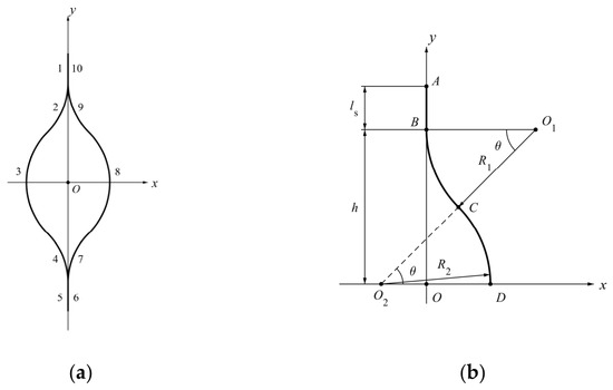
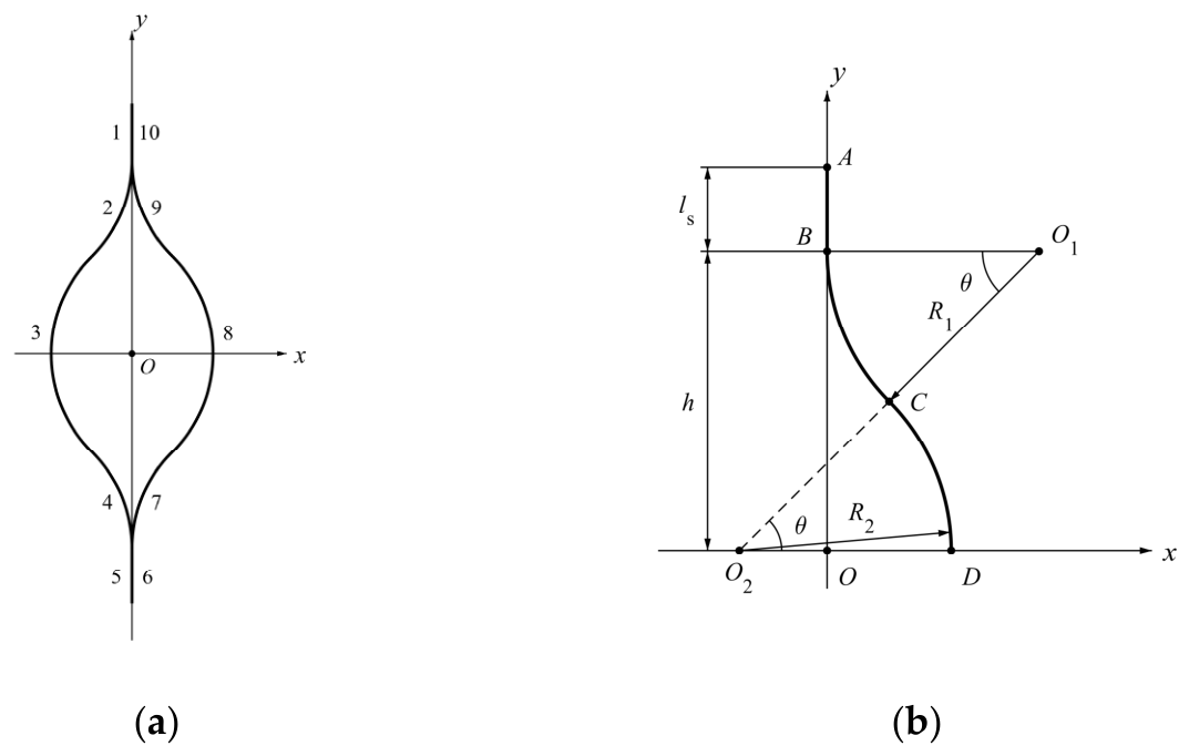
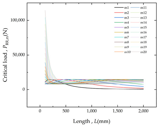
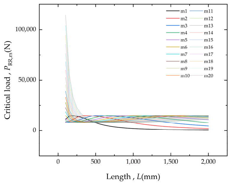
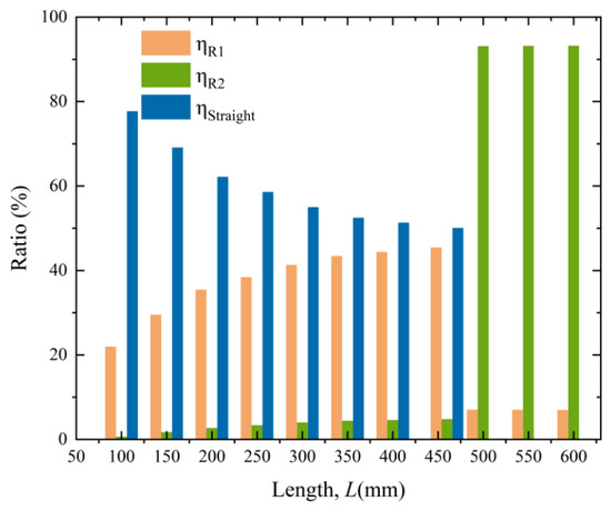
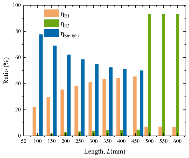
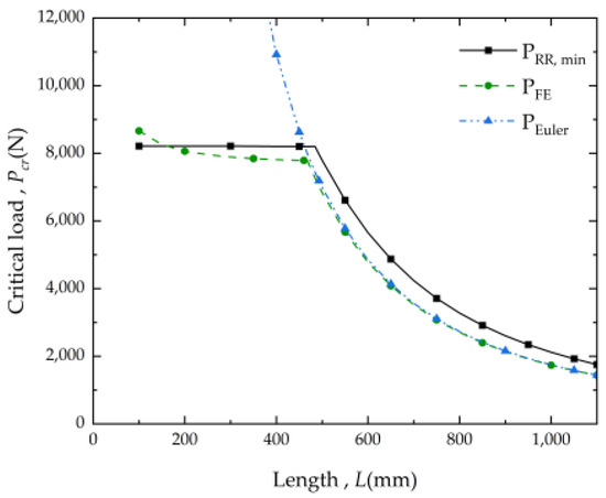
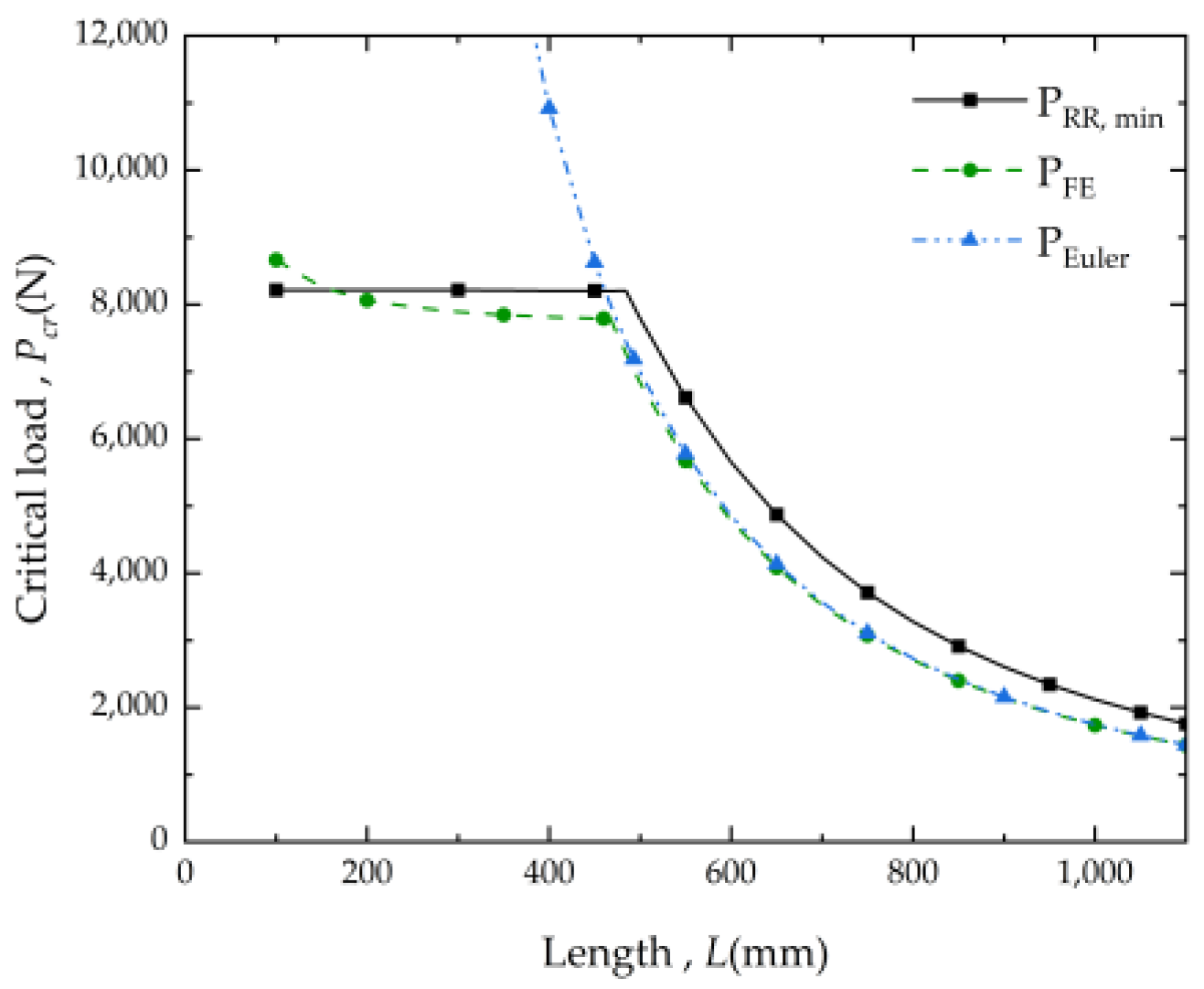
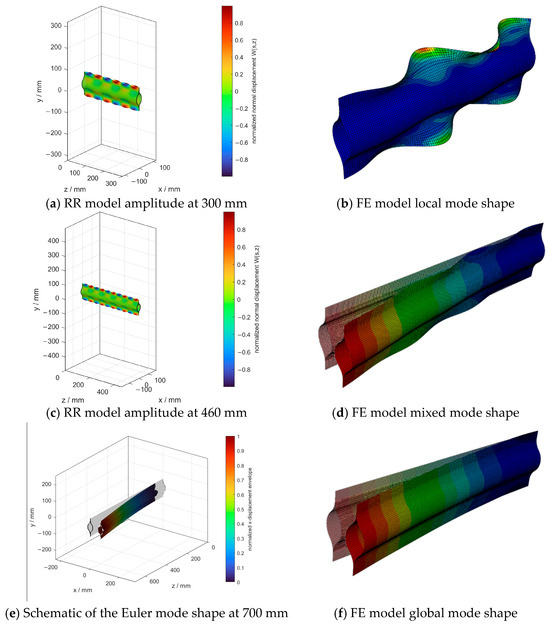
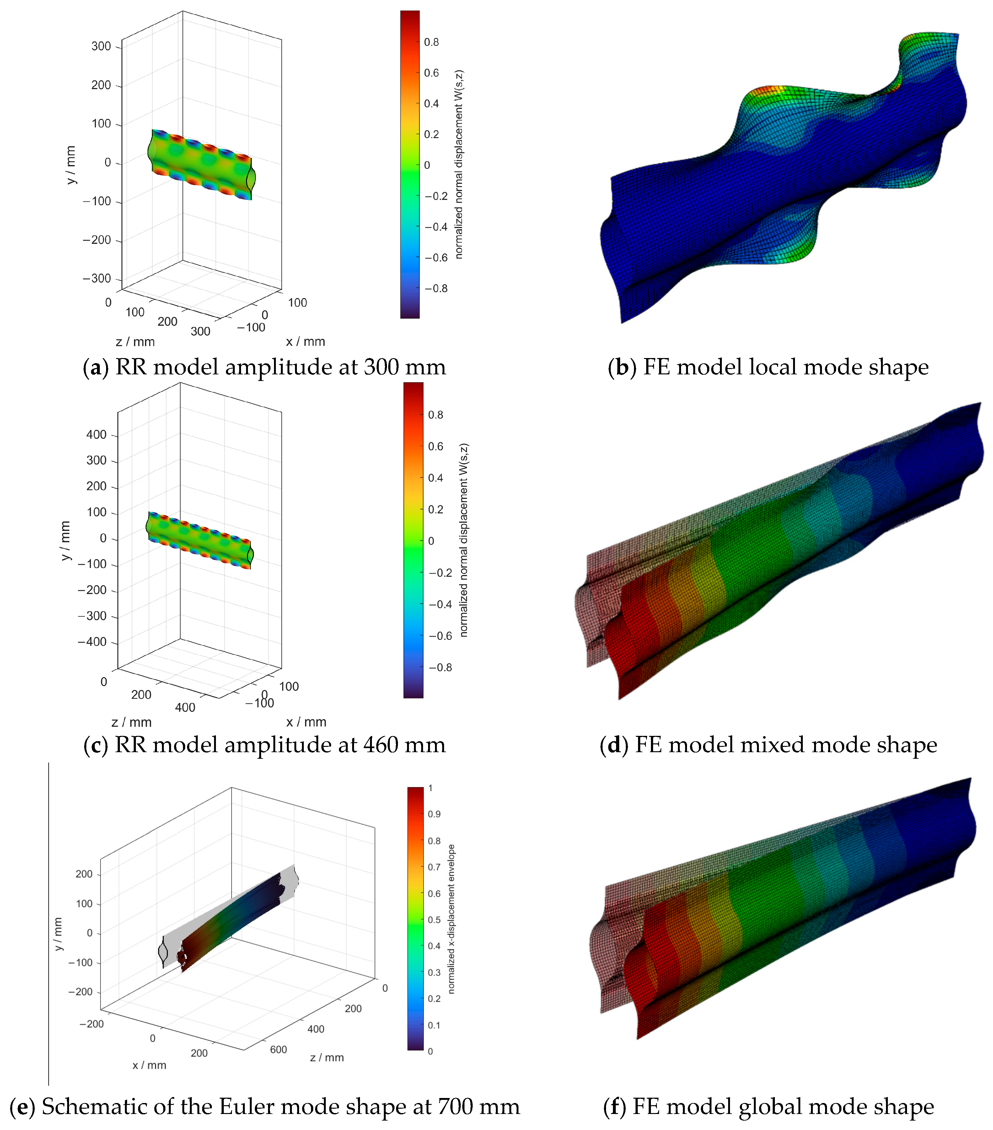
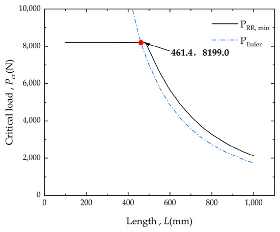
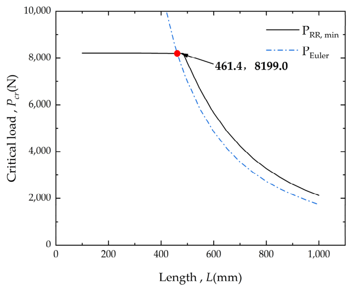
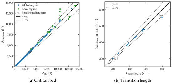
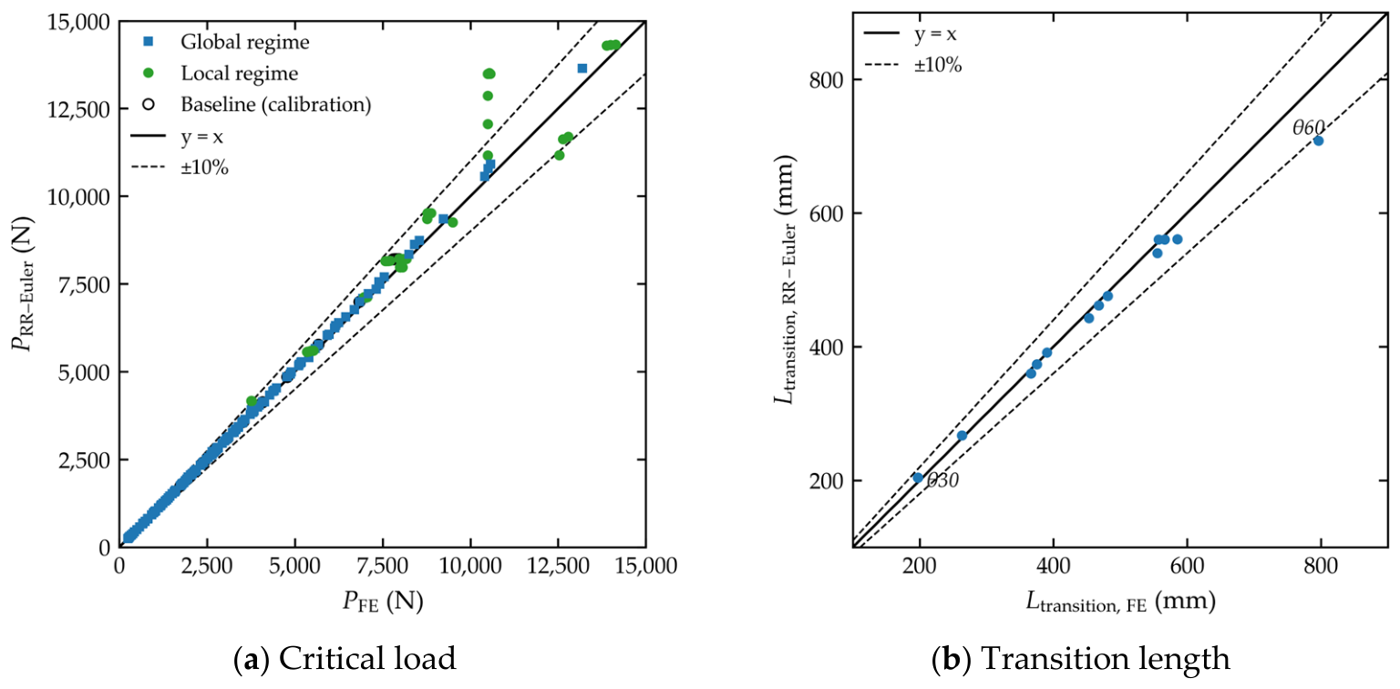
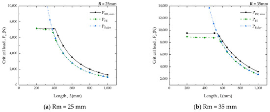
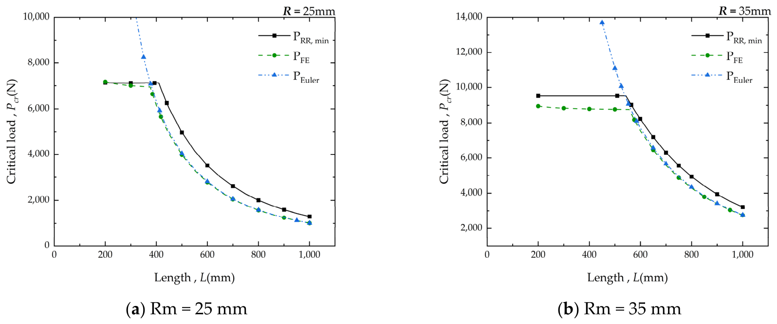
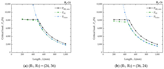
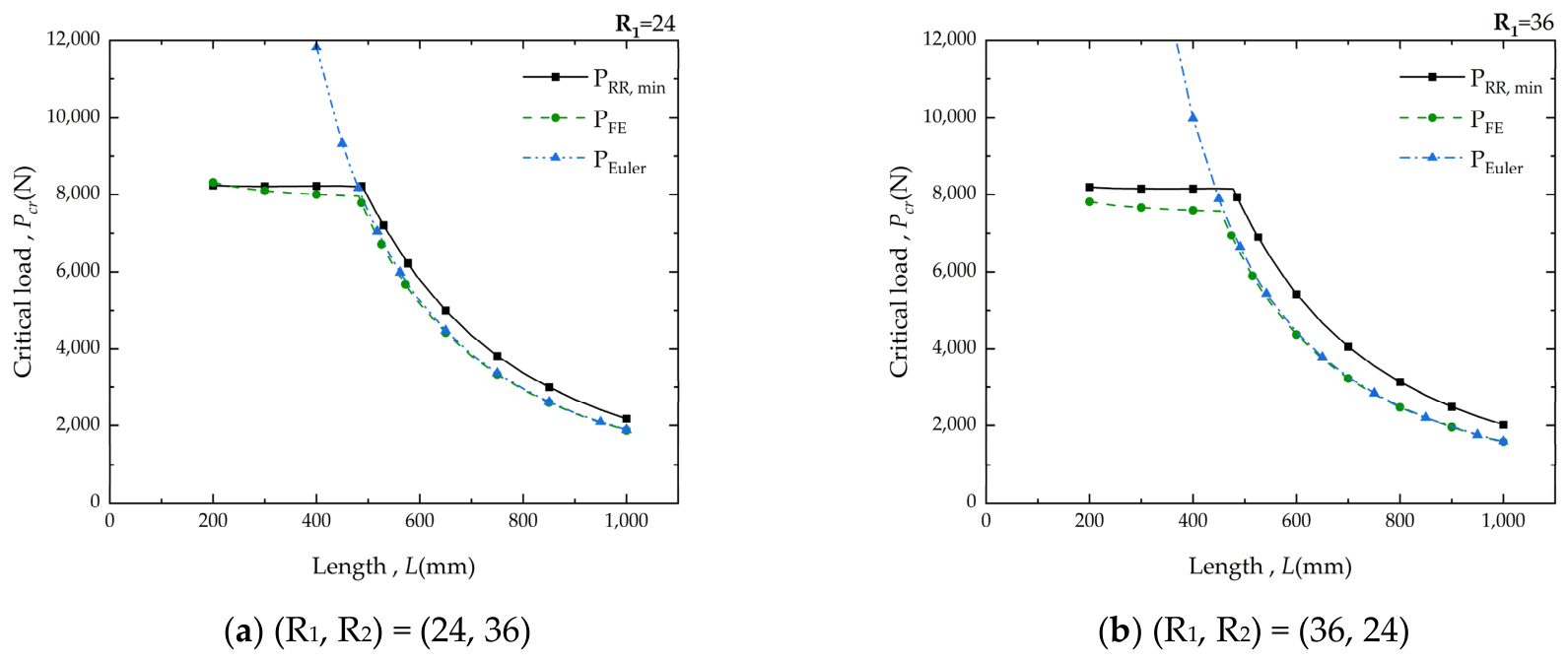
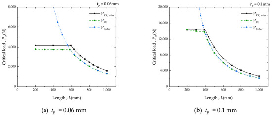
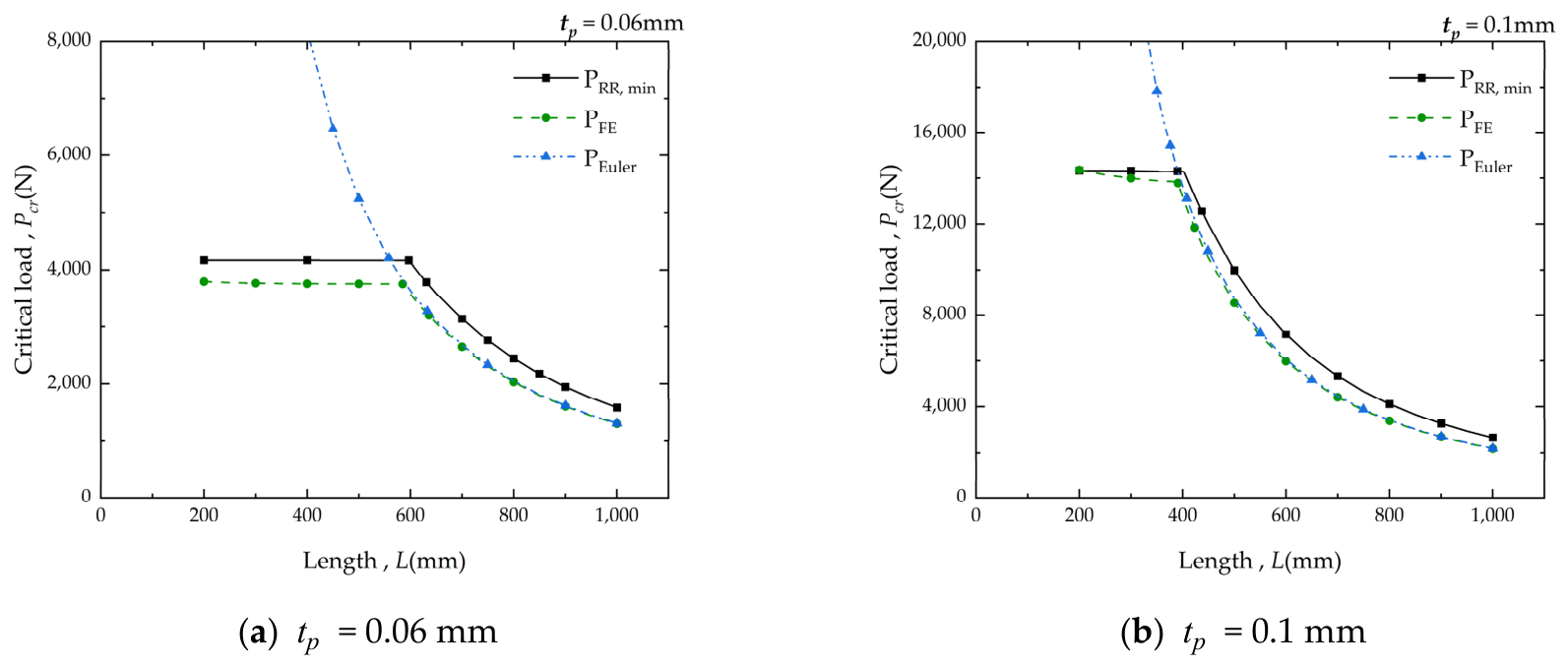
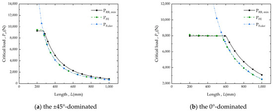
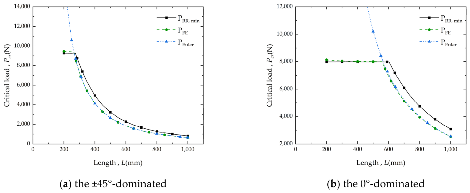
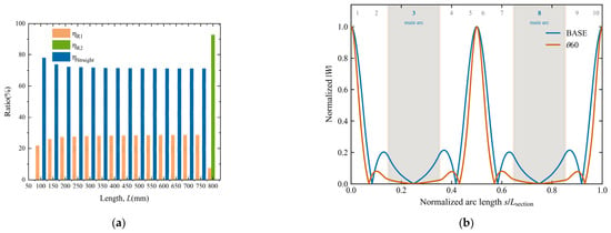
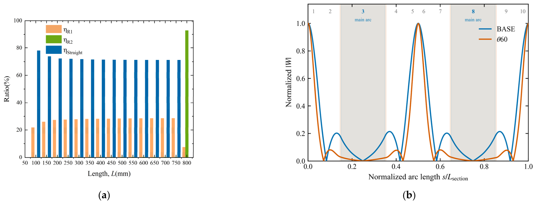

Disclaimer/Publisher’s Note: The statements, opinions and data contained in all publications are solely those of the individual author(s) and contributor(s) and not of MDPI and/or the editor(s). MDPI and/or the editor(s) disclaim responsibility for any injury to people or property resulting from any ideas, methods, instructions or products referred to in the content. |
© 2026 by the authors. Licensee MDPI, Basel, Switzerland. This article is an open access article distributed under the terms and conditions of the Creative Commons Attribution (CC BY) license.