


Abstract
Accurate prediction of traffic load generated by remote sensing tasks plays an increasingly important role in enabling LEO satellite networks to provide global observation and communication services. However, due to the highly dynamic topological structure and periodic variation characteristics of LEO, traditional traffic prediction methods often fail in scenarios with topology switching. Meanwhile, rolling prediction methods are prone to introducing error accumulation, making it difficult to ensure the stability of long-term prediction. To address these issues, this paper proposes a traffic prediction algorithm based on a Dynamic-Indexed Temporal Graph Convolutional Network (DI-TGCN). The proposed scheme integrates a graph convolutional network (GCN) and a gated recurrent unit (GRU) to form the base temporal graph convolutional network (TGCN), where the GCN captures spatial correlations and the GRU captures temporal correlations. A dynamic topology indexing mechanism is then introduced into TGCN, enabling each time step to automatically match the corresponding adjacency matrix, thereby realizing traffic prediction under topology switching. In the prediction phase, the model adopts a supervised multi-step prediction strategy that can directly output results for multiple future time steps in a single forward pass, mitigating the recursive error propagation of rolling prediction. Experiments on a simulated Iridium constellation of 66 satellites show that DI-TGCN outperforms CNN-LSTM, GCN, TGAT, and TGCN across prediction horizons from 15 to 120 min, reducing the RMSE by 7.2% to 10.5% compared with TGCN and maintaining an accuracy above 0.90 at all horizons, while its time complexity is almost the same as that of the static-topology TGCN (3.19 ms versus 3.15 ms per batch). These results demonstrate that the proposed scheme achieves accurate and efficient spatiotemporal traffic prediction for satellite networks with topology switching.
1. Introduction
In recent years, with the rapid development of Low Earth Orbit (LEO) satellite communication technology [1], satellite internet has gradually become an important part of global remote sensing applications. Large-scale LEO satellite constellations, such as Starlink and OneWeb [2], have been successively deployed, enabling global seamless communication with space–ground integration [3]. These satellites collect massive amounts of remote sensing data, which need to be transmitted to ground stations or other satellites [4,5]. Predicting the traffic load generated by such data transmission in LEO satellite networks has become a topic of widespread attention [6]. On one hand, traffic prediction technology can predict future traffic patterns based on historical traffic sequences, considering the specific connection relationships of satellites [7]. This allows the network to proactively respond to traffic fluctuations, reduce congestion, and optimize load distribution [8,9,10]. It also enables the network to predict surges in traffic and adjust in time, thus improving the network’s adaptability [11,12]. With accurate traffic prediction, the system can anticipate potential congestion paths, proactively reschedule large data transfers, avoid delays, and ultimately improve the overall network efficiency and stability [13,14].
On the other hand, in practical applications, existing traffic prediction methods exhibit certain limitations when addressing the unique challenges of data transmission over satellite networks. A significant feature of LEO satellite networks is the dynamism of their topology. Unlike static terrestrial networks, the positions of satellites change over time, causing the network topology to be constantly evolving [15,16]. Due to the orbital characteristics of satellites, the connection relationships between nodes are not fixed. This dynamic topology makes traffic prediction more complex. Especially in cases where link loads between satellites are uneven [17], most of the global network traffic is concentrated within latitudes of 50 degrees, where traffic load can increase significantly due to geographical location and the concentration of communication loads [18]. Facing such dynamic changes, traditional time-series-based traffic prediction methods often fail to effectively capture the complex relationship between topology and traffic loads, leading to reduced prediction accuracy [6].
The issue of network traffic prediction has gained widespread attention in the field of computer networks, with extensive research conducted by experts. Early work revealed the self-similarity of traffic, providing a theoretical foundation for subsequent studies [19]. Prediction methods have evolved from early Poisson processes and Markov processes [20], incorporating traffic features such as self-similarity, long-range dependence, periodicity, and chaotic behavior [21]. These learning-based approaches have effectively improved performance in a variety of wireless scenarios [22,23,24].
Traditional time series forecasting methods, such as the AutoRegressive Integrated Moving Average (ARIMA) model [25] and the Holt–Winters [26] exponential smoothing method, are well suited for short-term prediction tasks. ARIMA relies on a combination of linear autoregression and moving average components and can effectively model patterns in stationary time series. The Holt–Winters method incorporates trend and seasonal components and therefore offers some adaptability for short-term traffic sequences with periodic fluctuations. However, both methods exhibit clear limitations when applied to the highly dynamic traffic patterns of satellite networks. Their reliance on linear correlations often prevents them from capturing complex statistical characteristics and nonlinear behaviors, resulting in reduced prediction accuracy. In contrast, decomposition-based models such as Prophet, represented by Meta [27], reconstruct data sequences with similar periodicity and trends by analyzing the periodicity of the data and deseasonalized trends.
In contrast, nonlinear models based on neural networks and deep learning exhibit stronger capabilities in capturing complex data features [28,29]. These models outperform traditional linear models. Especially in rapidly changing traffic sequences, the Generalized Autoregressive Conditional Heteroskedasticity (GARCH) model demonstrates superior prediction accuracy [30]. Hybrid models integrate various methods explored in [31,32]. They further enhance network traffic prediction by leveraging advances in deep learning [33]. LSTM [34] networks use gating mechanisms to address the gradient vanishing problem of traditional Recurrent Neural Networks (RNNs) [35]. They can effectively mine long-term temporal dependencies in satellite traffic. Gated recurrent unit (GRU) networks simplify the gating structure of LSTM [36]. They achieve accurate filtering and transmission of temporal information with fewer parameters. While reducing computational complexity, they can efficiently capture short-term fluctuations and long-range correlations in satellite traffic sequences.
In LEO satellite networks, one of the core issues in traffic prediction is how to accurately capture the spatial dependencies between nodes and the temporal dynamics of traffic data. Since the topology of LEO satellite networks exhibits periodic changes across different time steps, an important research question emerges: how to dynamically select distinct topological structures for traffic prediction and integrate topological information into the prediction model [37]. Currently, network traffic prediction research increasingly focuses on the spatial correlations between network nodes. This trend is particularly evident in satellite data networks [38].
In [39], a spatiotemporal traffic forecasting algorithm based on a graph convolutional network (GCN) and an attention mechanism, referred to as GLA, demonstrates strong performance in time series prediction. However, its model structure typically assumes that spatial relationships within the data remain static. Ding and Chen [40] and Yang et al. [41] propose traffic prediction methods based on temporal graph convolutional networks (TGCNs), which integrate GCN and GRUs to achieve improved forecasting performance. Standard GCN models are designed for static graphs and therefore struggle to accommodate the dynamic evolution of satellite topologies. In [42], local spatial features are extracted using convolutional neural networks (CNNs), and temporal patterns are captured with long short-term memory networks, but CNN models cannot adapt to changes in topological dependencies caused by satellite node mobility. Cai et al. [43] employs a GAN to enhance the modeling capability of traffic data distributions and uses LSTM networks to capture temporal dependencies, but does not explicitly model dynamic spatial topology. In [44], long-term temporal dependency learning is strengthened through Transformer architectures, and a GCN is utilized to extract spatial correlations. Other studies combine ARIMA for linear trend fitting with BPNN for nonlinear feature extraction [45].
The above studies are all conducted under the assumption of static satellite topologies, which does not align with the real characteristics of LEO satellite networks. The topology of satellite systems exhibits inherent dynamism and periodic variation, and these methods are therefore unable to handle graph structures that evolve over time. As a result, the models fail to capture the underlying patterns of topological change, leading to reduced prediction accuracy [46].
In [47], a TPDS-GAN leverages a seq2seq framework combined with graph generation and spatial attention modules to predict dynamic traffic. This method dynamically generates adjacency matrices based on traffic attributes and utilizes spatial attention to adaptively learn neighbor feature weights. However, the generated dynamic adjacency matrix focuses on logical node correlations rather than the actual periodic physical topology switching. Consequently, the model struggles to capture time series rules effectively, leading to instability during rapid topological changes [48]. A structured comparison of the representative works discussed above is provided in Table 1.
Table 1.
Comparison of representative traffic prediction methods.
Moreover, traditional prediction methods often use iterative prediction strategies in multi-step prediction scenarios, where the previous prediction is used as input for the next step [49]. However, this leads to the gradual accumulation of errors, and the longer the prediction horizon, the larger the bias. Once the error accumulates to a certain extent, prediction collapse occurs. In satellite networks, traffic prediction often needs to span from fifteen minutes to several hours. Therefore, mitigating the accumulation of iterative prediction errors is an important issue that this paper aims to address [50].
As far as we know, the problem of predicting traffic load for remote sensing data transmission under topology switching in satellite networks still requires effective research. To address this issue, we introduce a novel method called a Dynamic-Indexed Temporal Graph Convolutional Network (DI-TGCN). It is worth emphasizing that, benefiting from the deterministic orbital mechanics of LEO constellations, the topology at any future time step can be pre-computed from orbital ephemeris rather than learned from data. The DI-TGCN exploits this prior knowledge: it retrieves the known future topology states through a deterministic index and predicts the traffic load under the corresponding topology. Our key contributions can be outlined as follows:
- (1)
- We propose the Dynamic-Indexed Temporal Graph Convolutional Network. This model can simultaneously capture the spatiotemporal characteristics in satellite networks. It is well-suited for satellite traffic data with complex spatiotemporal dependencies. By exploiting the fact that future topology states are deterministically pre-computable from orbital ephemeris, it enables accurate traffic load prediction under the highly dynamic topological structure of LEO satellite networks.
- (2)
- To address traffic prediction under topology switching in satellite networks, this paper proposes a dynamic topology indexing mechanism. This mechanism enables the model to automatically select the corresponding topological structure for each time step. It resolves the limitation of a single fixed topology in traditional TGCN models. Thus, it effectively models the spatiotemporal dependencies under topology switching.
- (3)
- We propose a direct multi-step prediction module based on supervised learning. This module can directly output prediction results for multiple future time steps in a single forward propagation. Compared with traditional rolling prediction methods, it mitigates the problem of prediction errors propagating and compounding across steps. Thus, the model can maintain higher accuracy and stability in long-term prediction tasks.
- (4)
- To verify the effectiveness of the proposed model, this paper generates a series of consecutive topologies of the Iridium constellation under real orbital conditions via simulation. Since real satellite traffic is confidential and inaccessible, terrestrial ISP traffic from a European core network is injected into the simulated constellation to construct the simulated satellite traffic, and the statistical characteristics of the constructed traffic are analyzed to verify the rationality of this construction. By comparison with other prediction methods, it fully demonstrates the advantages of the proposed method in traffic prediction tasks under the highly dynamic topological structure of satellite networks.
The structure of this paper is organized as follows. Section 1 examines the existing research on LEO satellite networks and traffic prediction methods. Section 2 elaborates on the system model of the research. Section 3 presents the overall workflow of the traffic prediction model based on the DI-TGCN and the method of data processing. Section 4 provides a detailed illustration of the composition and underlying principles of each module of the proposed model in this paper. Section 5 introduces the adopted dataset and experimental results, analyzes the underlying reasons, and verifies the effectiveness of the proposed algorithm. Section 6 summarizes the research findings of this paper and puts forward potential avenues for future research in this field.
2. System Model
As shown in Figure 1, LEO satellite constellations achieve communication with each other through inter-satellite links to facilitate the transmission of remote sensing data. Each satellite operates in its specific orbit, and due to the periodic nature of its orbital characteristics, the topological relationships between satellites can be pre-computed. In other words, the topology sequence is treated in this work as prior knowledge obtained from orbital ephemeris, rather than as a random variable to be predicted; the prediction target of this study is the traffic load under each known topology. Specifically, each satellite communicates via up to 4 inter-satellite links; satellites in the same orbital plane are interconnected through intra-orbital links (solid lines), while neighboring orbital planes communicate through inter-orbital links (dashed lines). The length and connectivity of inter-orbital links change periodically with the satellites’ motion, so the number of links between each satellite and others varies between 2 and 4. For simplicity, we ignore the reverse stitching factors in the satellite constellation, resulting in the grid topology shown in Figure 1.
Figure 1.
Satellite network topology diagram.
The problem of satellite network traffic prediction can be formalized as a spatiotemporal sequence prediction task. The satellite network topology is modeled as an undirected graph represented as , where represents the set of nodes corresponding to the N nodes in the satellite constellation, represents the set of edges at time t reflecting the available links between satellites, and represents the adjacency matrix, with if satellite and satellite have an active link at time t and otherwise.
At each time step t, each network node will generate a certain amount of traffic demand that forms the feature vector, which is defined as
Let represent the traffic demand generated at node at time t. Given a fixed historical time window, we define the history window as
Our goal is to learn a prediction function, which can be formulated as
where H represents the forecast horizon, (with ) denotes the traffic demand feature vector of the satellite network at time , denotes the adjacency matrix characterizing the topological structure of the satellite network at time , and the model needs to predict the future traffic demand at time (with ) based on historical traffic demand () and network topology information (). The model predicts traffic demand for future time steps at the given nodes.
3. DI-TGCN
In Low Earth Orbit satellite communication networks, inter-node dependencies are not static but exhibit significant characteristics of periodic topology switching. Traditional Graph Neural Networks often assume a single fixed adjacency matrix. This static assumption causes the model to fail in capturing non-stationary spatial dynamics, which is inconsistent with reality and limits prediction accuracy.
To address this issue, we propose an end-to-end deep learning algorithm named DI-TGCN. The core design philosophy of this algorithm is topology-data synchronization awareness, aimed at establishing a spatiotemporal modeling mechanism capable of responding to constellation changes in real time. As shown in Figure 2, the structural workflow of DI-TGCN is illustrated. The Multi-Topology Temporal Weaving module is designed to address the challenge of data alignment within dynamic environments. By ingesting raw traffic features and topology period information, it reorganizes heterogeneous topological data streams into time-continuous composite sequences while synchronously generating a topology index sequence. This sequence serves as a critical control signal that is fed into the subsequent Selector. The Dynamic Topology Indexing Mechanism pre-constructs a topology bank containing normalized Laplacian matrices corresponding to all topological states. During both training and inference phases, the Selector utilizes the current topology index to retrieve and precisely inject the corresponding Laplacian matrix from the bank in real time. This ensures that the GCN performs convolution operations at each time step using structural information that is strictly consistent with the instantaneous physical topology. Subsequently, the GRU integrates these dynamic spatial features into its gating mechanism to capture temporal evolution patterns and long-short term dependencies, propagating the hidden state to the next time step. Finally, the Direct Multi-step Decoding module adopts a direct mapping strategy, where the model employs a fully connected layer to map the final hidden state directly to the multi-step prediction results.
Figure 2.
Framework flowchart of DI-TGCN.
3.1. Multi-Topology Temporal Weaving
The construction of the model begins with the pre-processing of non-stationary data streams. In our research scenario, we know the specific structures of various satellite constellation topologies. There are K predefined topological states, and the satellite constellation cycles through these states according to a fixed period P.
If traditional processing methods are adopted, such as directly mixing training data from different topologies or simply concatenating them by time, it leads to confusion in spatial context, meaning the model cannot distinguish which graph generated the current traffic data. Therefore, we designed an interleaved weaving strategy to construct the input tensor.
Specifically, the data loader does not view the time axis as a single-dimensional tiling but treats it as a sequence composed of multiple topology blocks. Each block contains P continuous time steps, corresponding to the operational data of the system within a complete topology cycle. The loader sequentially extracts data blocks from the corresponding topological raw feature sources and concatenates them according to the progression of physical time.
This mechanism not only generates a feature matrix matching the model from raw traffic data but, more critically, generates a topology index sequence. As a metadata label strictly synchronized with input features, this sequence indicates which specific topological state each time step belongs to. This provides an accurate signal for the subsequent neural network to perceive the current spatial structure, achieving strict spatiotemporal alignment between the data stream and the topology stream.
3.2. Multi-State Topological Graph Modeling
After obtaining aligned input data, the main issue lies in processing multiple heterogeneous graph structures within a single batch. Traditional GCN models rely on a static Laplacian matrix and cannot adapt to this changing structural requirement. To this end, we propose a GCN based on a dynamic Laplacian selection mechanism.
This module no longer relies on a single adjacency matrix but constructs a topology storage pool during the initialization phase, pre-computing and storing normalized Laplacian matrices for all K states.
During forward propagation, the module introduces sample-level dynamic topology indexing. Utilizing the topology index sequence generated in the previous section, the model can retrieve its exclusive Laplacian matrix via indexing for each sample in the same batch and for each time step within the same sample. Subsequently, through batch matrix multiplication, the model achieves feature aggregation on different graph structures for different samples within the same operation. This mechanism ensures that every convolution operation strictly follows the real physical connection relationship at the current moment, guaranteeing the physical authenticity of spatial feature extraction.
Although the underlying connection structure jumps continuously, the dynamic laws of traffic diffusion between nodes often possess cross-topology commonalities. To capture this universal pattern and prevent overfitting, we share the feature transformation matrix across all topological states.
This design of dynamic structural switching and global parameter sharing enables DI-TGCN to possess both the flexibility to adapt to environmental changes and strong generalization capabilities, allowing it to learn robust spatial evolution laws from limited data.
3.3. Topology-Aware Spatiotemporal Fusion
Isolated spatial features are insufficient to describe the full picture of the system and must be placed on the time axis for dynamic evolution. We embed the aforementioned dynamic graph convolution unit into the GRU to construct a spatiotemporal fusion layer.
In a standard RNN, the update of the hidden state relies only on a linear fully connected layer, ignoring the influence of spatial structure on memory updates. In DI-TGCN, we completely replace the matrix multiplication inside the GRU with dynamic interaction graph convolution operations. Specifically, the generation of the spatially aware Reset Gate and Update Gate depends not only on the memory of the previous moment but also on the state of neighbor nodes under the current specific topology at the current moment. This means that the gating mechanism itself possesses spatial filtering capabilities, dynamically adjusting the forgetting and retention of information based on local network loads. Furthermore, in dynamic context fusion, when calculating the candidate hidden state, the model calls the dynamic graph convolution again to aggregate the current input features with the reset historical memory on the current graph structure.
Through this hierarchical recursion, DI-TGCN essentially completes a spatial diffusion on a specific dynamically changing graph at every time step, using the diffusion result as a driving force to propel the time sequence to the next step. After processing through the encoder window length, the hidden state vector of the last time step encapsulates complex spatiotemporal interaction information within the entire historical window.
3.4. Multi-Horizon Output
The ultimate goal of spatiotemporal modeling is the precise prediction of future states. In complex scenarios with topology switching, traditional rolling recursive prediction is difficult to adapt. In such recursive schemes, the prediction of the previous step is fed back as the input of the next step; once a deviation occurs, it couples with the switched spatial context of subsequent steps and is gradually amplified, which can trigger a chain reaction of prediction collapse.
To solve this problem, DI-TGCN abandons the recursive mode and adopts the direct multi-step prediction paradigm as the core strategy of the output layer.
We regard the high-dimensional hidden state output by the spatiotemporal fusion layer as a complete expression of the latent space. The output layer consists of a fully connected linear projection layer, which directly establishes the mapping relationship from the hidden dimension to future predictions.
For each node, the decoder outputs prediction vectors for H continuous future time steps in parallel at once. Mathematically, this process can be expressed as
where is responsible for transforming the feature dimension into the time step dimension.
Adopting the direct output strategy can cut off the error propagation chain. The model prediction for time is completely independent of the prediction result for time . This means that short-term local fluctuations or prediction deviations will not be carried over and amplified into long-term predictions, greatly enhancing the robustness of the model in dynamic environments. During the training process, the loss function supervises and optimizes the future H steps as a whole trajectory. This forces the model to learn the intrinsic correlations between time steps, generating prediction curves that are smoother in trend and consistent with physical laws. Additionally, this strategy requires only one forward pass during the inference phase, significantly reducing the time complexity of prediction, making it highly suitable for online monitoring tasks with high real-time requirements.
Through the above processes, DI-TGCN successfully constructs a closed-loop dynamic spatiotemporal prediction mode. It not only achieves precise adaptation to the topological structure of every time step but also ensures the stability of long-term prediction through direct multi-step decoding, providing a theoretical paradigm for solving multi-mode dynamic graph prediction problems.
4. Module Design
4.1. Dynamic Topology Indexing Mechanism
In this paper, dynamic topology refers to the time-varying connectivity of the constellation, topology switching denotes the transition between topology snapshots, and dynamic topology indexing denotes the retrieval of the snapshot associated with each time step.
As the structural navigation unit of the proposed DI-TGCN framework, the dynamic topology indexing mechanism is designed to resolve the spatial mismatch problem caused by the rapid orbital movement of LEO satellites. Unlike traditional static approaches that rely on a fixed graph, this mechanism functions as the foundational layer of our spatial encoder, allowing the neural network to dynamically perceive and retrieve the correct topological context corresponding to the current input data stream.
To support the real-time structural adaptation of DI-TGCN, we first construct a topology storage pool during the initialization phase to persist the discrete structural states of the constellation. Specifically, representing the node set V at time step t with an adjacency extension, the system stores the continuous K snapshot extensions of the satellite constellation as
where K represents the total number of defined topology states and each matrix corresponds to the specific physical connection pattern during a distinct orbital phase. Within the DI-TGCN architecture, this storage pool ensures that when a link between satellite A and satellite B breaks due to orbital dynamics, the model can instantly switch to a valid graph view without structural ambiguity. To drive the subsequent graph convolution operations, the mechanism generates a synchronization signal known as the topology index as
which explicitly instructs the spatial encoder to utilize the k-th Laplacian matrix for feature aggregation at the current moment.
Furthermore, to align this indexing logic with the Multi-Topology Sequential Weaving strategy of DI-TGCN, we incorporate the periodicity of satellite orbits into the index generation process. By dividing the continuous time axis into periodic blocks of length P, the mechanism ensures that the topology state remains consistent within each calculation window, thereby reducing redundant switching operations and maintaining context stability for the GRU module. Mathematically, to realize this periodic alignment during the rolling prediction process, the model first calculates the relative position within a topology cycle as
where denotes the periodic time segment corresponding to the global time step t. Consequently, the specific topology index driving the DI-TGCN encoder at step t is derived as
which ultimately maps to the retrieval of the context-aware adjacency matrix as
ensuring that the calculation of spatial dependencies in DI-TGCN is always consistent with the real-time physical network topology. This rigorous indexing mechanism not only guarantees the physical authenticity of the spatial features extracted by the model but also provides DI-TGCN with the scalability to handle complex constellations by simply updating the snapshot list.
We now clarify the distinction between the proposed indexing mechanism and existing dynamic-graph approaches. Methods such as EvolveGCN, DySAT, and the TPDS-GAN in [47] address scenarios where the graph evolution is unknown and must be learned from data. They either evolve model parameters over time or generate adjacency matrices from traffic attributes. The learned adjacency reflects logical node correlations rather than the actual physical inter-satellite links, and the extra learning process introduces both estimation errors and computational overhead. In our scenario, however, the constellation topology is known a priori and switches periodically, so estimating the graph from data is unnecessary and would only inject additional errors. The dynamic topology indexing mechanism is designed under this observation, and its contribution is threefold. First, it performs sample-level and step-level retrieval of pre-computed normalized Laplacian matrices, so that a single model can be trained on interleaved multi-topology data without confusing the spatial context of different snapshots. Second, the indexing adds no learnable parameters and almost no extra inference cost, which is verified by the efficiency evaluation in Section 5.5. Third, together with the cross-topology shared weight matrix, it forces the model to learn universal traffic diffusion patterns rather than overfitting to any single snapshot. The indexing mechanism is therefore the key component that enables a static-graph TGCN to exploit the deterministic constellation prior knowledge.
4.2. Dynamic-Indexed GCN
As the spatial encoding engine of DI-TGCN, the dynamic graph convolutional network is specifically designed to address the fluctuating non-Euclidean spatial dependencies induced by satellite orbital motion. As illustrated in Figure 3, traditional GCN models rely on a single static graph structure and cannot accommodate the irregular and time-varying connections of LEO constellations. The dynamic-indexed GCN uses index signals to select the Laplacian matrix matching the instantaneous physical environment for graph convolution during information aggregation. This design enables the model to achieve precise spatial feature aggregation under topology switching. By mapping the real-time topology retrieved via the dynamic topology indexing mechanism onto the graph model, DI-TGCN ensures that node interactions are conducted through the actual physical links present at any given moment. This effectively constructs a graph model that reflects the authentic spatial topology of the network, thereby preserving the global correlations among satellites.
Figure 3.
Neural architecture of the dynamic-indexed GCN.
To mathematically represent the connectivity within a specific topology snapshot, we first utilize an adjacency matrix to describe the relationships between N satellite nodes as
which works in conjunction with a degree matrix where each element represents the connectivity density of each node. However, to translate the dynamic topology index defined in the previous section into actual computational operators, we no longer rely on a single static matrix but construct a pre-computed normalized Laplacian matrix pool based on topology snapshots as
where each element corresponds to the normalized spectral operator for a specific orbital phase. Under this mechanism, for any given time step t, the model retrieves the precise Laplacian matrix for the current moment by querying the dynamic topology indexing mechanism as
which explicitly instructs subsequent convolution operations on which graph structure to base their computations. To process the input feature matrix containing traffic attributes of dimension C, the module fundamentally relies on graph signal propagation in the spectral domain. Based on the currently selected graph structure (denoted as L hereafter to simplify the derivation), it is defined as
For spectral analysis, the Laplacian matrix is decomposed as
where U is the eigenvector matrix and is the diagonal matrix of eigenvalues, followed by the definition of the graph Fourier transform of signal x as
and its corresponding inverse transform is expressed as
which allows us to define the spectral convolution operation within the DI-TGCN encoder as
interpreting the process as the multiplication of the signal x and the learnable graph filter in the Fourier domain. However, calculating the eigen-decomposition for every topology switch in our dynamic environment is computationally prohibitive; therefore, DI-TGCN employs Chebyshev polynomials to efficiently approximate the filter, defining the approximated convolution as
where denotes the k-th order Chebyshev polynomial and is the rescaled Laplacian matrix retrieved via indexing. To further simplify dynamic computation while preserving spatial locality, we limit to adopt a first-order approximation, formulating the core aggregation rule of our spatial layer as
where represents the self-loop augmented adjacency matrix selected by the dynamic topology indexing mechanism at time t, and W is the trainable weight matrix shared across all topological states to learn universal traffic patterns. This operation signifies that DI-TGCN updates each node’s representation by aggregating weighted information from its current physical neighbors. To capture broader spatial dependencies across the satellite network, we stack multiple such dynamic layers and explicitly utilize the indexing mechanism to drive hierarchical propagation, defining the process from layer l to as
where denotes the node features at layer l at time t, and is the non-linear activation function. Through this index-driven multi-layer propagation mechanism, the final output not only encapsulates high-order spatial features that accurately reflect the current network state but also provides a structurally aligned input for the subsequent Gated Temporal Mechanism.
4.3. Spatiotemporal Fusion Gate
To input the spatial features extracted in the previous section into the continuous temporal evolution process, DI-TGCN introduces a specialized Spatiotemporal Fusion Layer, constructing the TGCNCell by embedding dynamic graph convolutions into a Gated Recurrent Unit. Unlike traditional Recurrent Neural Networks that ignore structural changes, this design utilizes the Dynamic Topology Indexing Mechanism as a bridge, ensuring that the memory update process strictly adheres to the real-time physical connectivity of the satellite network. Specifically, to calculate the state transition at time step t, the model first identifies the current structural context index b based on the previously established indexing logic as
which triggers the retrieval of the corresponding operator from the Laplacian pool to drive the gating operations. Within this structure-aware context, we inject the input and the hidden state at the previous moment into the joint computation of the reset gate and update gate as
where GraphConv denotes the dynamic spectral convolution operation we defined in the preceding subsection. This formulation ensures that the gating mechanism dynamically filters historical information based on the current connectivity pattern, following which we utilize this structured gating signal to construct the current candidate hidden state as
which similarly leverages the index-specific Laplacian matrix to aggregate current neighborhood features. Ultimately, DI-TGCN executes the final hidden state update by fusing the historical memory and the current candidate state in a proportion determined by the update gate as
a process that allows the model to retain historical information when is large while relying more on dynamic inputs during moments of drastic topological change. Formally, this recursive process in the time dimension can be encapsulated as the unique state evolution function of DI-TGCN, expressed as
where represents the gated graph convolution update function driven by the current topology index. When the topology of the satellite network evolves over time, this mechanism automatically switches to keep spatial information aligned with time steps, ensuring that the network correctly captures flow dependence features between nodes even amidst frequent physical link transitions, thereby achieving cross-topology spatiotemporal prediction.
4.4. Direct Multi-Step Prediction
As the terminal decoding component of the DI-TGCN architecture, the Direct Multi-step Prediction Strategy is designed to mitigate the risk of error accumulation inherent in traditional recursive prediction, particularly within dynamic topological environments. Given that the structure of the satellite network switches periodically with the orbit, a minor deviation in single-step recursion could couple with an incorrect topological context in subsequent steps, causing prediction errors to escalate dynamically; therefore, we adopt a one-shot forward mapping mechanism to directly project the high-dimensional spatiotemporal states extracted by the encoder into a complete output trajectory for H consecutive future time steps.
To formalize this process, we first define the traffic sequence of the past T time steps, which has been aligned by our multi-topology weaving strategy, as
and represent the corresponding sequence of structural snapshots retrieved by the dynamic topology indexing mechanism as
where denotes the node features and represents the physical adjacency relationships verified by the indexer. The encoder of DI-TGCN jointly encodes these inputs through the aforementioned dynamic graph convolution and spatiotemporal gating mechanisms to obtain the last-layer hidden state , encapsulating the context of the entire historical window. Subsequently, the decoder utilizes a fully connected regression layer as a mapping operator to output the prediction sequence for H future time steps in parallel as
where represents the overall mapping function of the model from the input space to the future prediction space, and denotes the set of all learnable parameters, including the Laplacian pool, graph convolution filters, and the regression layer. This supervised direct decoding strategy integrates seamlessly with our dynamic adjacency matrix sequence, removing the recursive propagation path of errors across different topological states, which helps improve the stability of long-sequence prediction under the dynamic structural changes of satellite constellations.
4.5. DI-TGCN Training Procedure
The proposed DI-TGCN model focuses on accurate traffic prediction under topology switching in satellite networks. This model accepts several consecutive topology snapshots of the constellation and the corresponding historical traffic matrices as input, and generates the predicted traffic matrix under the corresponding topology states as output. The overall system structure of the model is shown in Figure 4, which combines TGCN with the dynamic topology indexing mechanism to achieve efficient prediction of network traffic data.
Figure 4.
Overall system structure of DI-TGCN.
In the process of model construction, the network traffic matrix sequence is first normalized and preprocessed. This includes constructing the traffic feature matrix based on the real network topology and normalizing it. The input data is processed through two synchronized streams. On the structural stream, the Laplacian Matrix Pool Precomputation module pre-constructs all topology snapshots. On the data stream, the historical traffic series serves as the input payload.
These data streams converge at the Dynamic Topology Indexing module. This critical component utilizes time step information to identify the current topology index, retrieves the corresponding pre-computed Laplacian matrix from the pool, and matches it with the current traffic data, enabling the model to aggregate traffic and node information under the correct topology.
The matched topological structure and traffic data are immediately fed into the TGCNCell. Within the cell, the retrieved Laplacian matrix drives the dynamic graph convolution operations embedded in the GRU gates: the reset gate and update gate are produced by a graph convolution over the current input and the previous hidden state , and the candidate hidden state is computed by a second graph convolution over and the gated memory . In this way, spatial feature extraction is performed inside the gating mechanism at every time step, strictly following the instantaneous physical topology. Finally, the hidden state of the last time step is projected through the Fully Connected Layer for direct multi-step forecasting, generating prediction results in a single forward pass.
The detailed training procedure of the DI-TGCN algorithm is presented in Algorithm 1.
| Algorithm 1 Training Procedure of DI-TGCN |
| Require: Historical traffic sequence , Topology snapshots , Topology Period P Ensure: Trained DI-TGCN model parameters 1: Phase 1: Initialization & Precomputation 2: Construct the Laplacian Matrix Pool 3: Preprocess to generate aligned samples containing 4: Split data into training set and test set 5: Initialize model parameters randomly 6: Phase 2: Model Training 7: for epoch to E do 8: for each batch in do 9: Step 1: Dynamic Index Adaptation 10: Retrieve structural sequence via Indexing 11: Initialize hidden state 12: Step 2: Spatiotemporal Encoding (TGCNCell) 13: for to T do 14: Extract current matrix from 15: Reset / update gates (Equation (22)): 16: 17: Candidate state (Equation (23)): 18: 19: Hidden state update (Equation (24)): 20: 21: end for 22: Step 3: Direct Multi-step Decoding 23: Generate predictions 24: Optimization 25: Compute Loss 26: Update 27: end for 28: end for 29: return Optimized Model and prediction results |
5. Simulation and Performance Analysis
In this study, simulation experiments and analyses of results for the traffic prediction model based on the Dynamic-Indexed Temporal Graph Convolutional Network (DI-TGCN) were conducted on a Windows 11 64-bit operating system. The implementation utilized the PyTorch 2.5.1+cu121 deep learning framework and the Python 3.12 programming language, accelerated by an NVIDIA RTX 4060 GPU. The experiments employed real-world network traffic data combined with simulated satellite topologies.
5.1. Dataset
The experimental data utilized in this paper comprises two distinct components: real-world network traffic data and simulated satellite topology data.
Due to the high confidentiality [51] and limited accessibility of actual satellite traffic data, this study constructs simulated satellite traffic based on terrestrial network data. The raw dataset originates from a European core network operator (ISP) [52], covering transatlantic link traffic from 7 June 2005 to 31 July 2005, with a sampling interval of 5 min. The data format consists of timestamp–traffic value pairs.
The rationality of this construction is supported by the statistical comparability between terrestrial backbone traffic and satellite-borne data traffic, since both exhibit self-similarity, long-range dependence, and pronounced diurnal periodicity [19,21], and our measurements on the constructed traffic confirm these properties quantitatively (Figure 5). This practice is also consistent with prior satellite traffic prediction studies, which resort to simulated constellations together with synthetic or terrestrial traces because real in-orbit satellite traffic is classified and publicly unavailable [44,53].
Figure 5.
Statistical characterization of the simulated satellite traffic. (a) Traffic traces over two weeks. (b) Autocorrelation function with 24 h periodicity. (c) Variance–time plot for Hurst parameter estimation.
We extracted the hour field from the timestamp of each traffic record. To ensure data coverage and simulate traffic variations across different time periods, we defined the hours from 09:00 to 21:00 as peak periods, during which 300 source–destination node pairs were randomly selected. The remaining hours were designated as off-peak periods, with the number of node pairs reduced to 200. In every period, all 66 satellite nodes were covered.
Utilizing the timestamped traffic values from the raw data, traffic injection was performed on the satellite topology at every 5 min time step. Routing was executed on the adjacency matrix based on the shortest path algorithm. The shortest path algorithm is adopted to route the injected flows for the following reasons. On the one hand, shortest-path forwarding is the baseline routing principle widely used in existing satellite routing protocols, since the limited onboard processing and storage capability of satellites favors deterministic and lightweight routing decisions, and shortest-path forwarding remains the default routing assumption in LEO constellation simulation studies [44,53]. Since this work focuses on traffic prediction rather than routing optimization, adopting this standard baseline routing policy keeps the constructed traffic consistent with mainstream simulation practice and avoids introducing additional routing-policy bias into the dataset. On the other hand, the random selection of source–destination pairs is intended to traverse as many potential traffic distribution cases as possible. In each simulation period, different node pairs are randomly chosen as traffic sources and destinations, so that the injected flows cover diverse geographic regions and load levels over the whole simulation. This design prevents the constructed traffic from reflecting only a single fixed distribution pattern, and better mimics the spatial uncertainty of real satellite traffic, where user locations and service requests vary continuously over time. The load of each satellite was calculated as the sum of data processed during each injection event. For a single satellite, its resulting traffic sequence is illustrated in Figure 6. This data authentically reflects the periodic characteristics of network traffic, indicating the feasibility of predicting this sequence.
Figure 6.
Traffic trends of satellite nodes.
To examine the statistical characteristics of the constructed traffic, Figure 5 presents the traffic traces, the autocorrelation function, and the variance-time analysis. The aggregate and per-node traces exhibit pronounced diurnal fluctuations (Figure 5a), and the autocorrelation function decays slowly with distinct peaks at lags corresponding to 24 h (Figure 5b), indicating long-range dependence superimposed on daily periodicity. Using the aggregate-variance (variance-time) method, the estimated Hurst parameter is for the aggregate series and at the node level. The rescaled-range (R/S) method yields consistent estimates of and , respectively. These values fall within the range typically reported for self-similar Internet and satellite network traffic [19], confirming that the simulated satellite traffic possesses the same long-range dependent structure that a satellite traffic predictor is required to capture.
For each timestamp, a one-dimensional traffic vector for all nodes is generated. As time progresses, an traffic matrix is obtained, where M is the number of valid timestamps and is the number of nodes. Mathematically, this traffic matrix can be expressed as
The number of rows M in the matrix represents the number of time steps, and the number of columns N represents the number of nodes. Each element represents the flow of the n-th node at the m-th time step.
Simultaneously, the adjacency matrix of the corresponding topology snapshot is paired with it to form the complete spatiotemporal input data.
The satellite topology was generated using Systems Tool Kit (STK) simulation, as shown in Figure 7. First, the layout and orbital parameters of the Iridium constellation, comprising 66 nodes, were configured as shown in Table 2. Then, a sequence of adjacency matrices was generated based on the visibility constraints of inter-satellite links.
Figure 7.
STK three-dimensional simulation of the Iridium constellation.
Table 2.
Satellite constellation and topology snapshot configuration.
Given the scalability of our proposed method, demonstrating experimental validity through representative scenarios is sufficient. Therefore, we pre-generated three typical topology snapshots, representing satellite connectivity states at different times. These topologies alternate periodically along the timeline, thereby forming a dynamic network structure. The detailed configuration of the topology snapshots is reported in Table 2. Each snapshot corresponds to a distinct simulation epoch in STK and remains valid for a topology period of time steps (i.e., 10 min, since the sampling interval is 5 min); the constellation therefore cycles through the snapshots with a switching cycle of min. This switching cycle is chosen to be shorter than the orbital period of the Iridium constellation (approximately 100 min) so that the model is exposed to multiple topology transitions within a single orbital revolution, which represents a more challenging setting than the real orbital evolution and thus suffices to validate the dynamic topology indexing mechanism. Inter-satellite link visibility in STK is determined by the standard constraints of the Iridium constellation: each satellite maintains two permanent intra-plane links with its fore and aft neighbors in the same orbital plane at a fixed distance of about 4030 km, and up to two inter-plane links with satellites in the adjacent planes, whose distance varies between 3270 km and 4480 km with latitude. Following the operational constraints of the Iridium constellation, inter-plane links are established only when line-of-sight visibility is satisfied and the two satellites are below a latitude of about 60°, and they are deactivated near the polar regions and across the counter-rotating seam.
5.2. Benchmark Method
To verify the effectiveness of the method proposed in this paper, we selected the following benchmark algorithms for performance comparison:
- CNN-LSTM (CL): CL is a hybrid model that combines convolutional neural networks with long short-term memory networks. The CNN component effectively extracts local spatial features, while the LSTM component captures temporal dependencies.
- GCN: GCN is a neural network designed for graph-structured data. It captures spatial dependencies between nodes through graph convolution operations.
- TGCN: TGCN integrates a GCN with a GRU. It uses the GCN to capture spatial relationships within the graph structure and employs the GRU to handle long-term dependencies in time series data.
- TGAT: TGAT is a spatiotemporal graph model that combines graph convolution with attention mechanisms. The self-attention mechanism enhances its capability to model long-term dependencies within spatiotemporal data.
To ensure a fair comparison, all models are evaluated under an identical experimental protocol: the same interleaved multi-topology feature sequence, the same training/test split (8:2), the same historical window (), and the same direct multi-step forecasting strategy with an identical prediction horizon. The prediction target of every model is the node traffic vector of the future H time steps. The models differ only in the topological information they are able to consume, as specified in Table 3: the baseline models are restricted to a single static topology snapshot (i.e., the topology index is fixed to 0), whereas DI-TGCN additionally receives the topology index sequence and the full snapshot set, and retrieves the corresponding Laplacian matrix at each time step through the dynamic topology indexing mechanism.
Table 3.
Input and forecasting strategy of each compared model.
It should be noted that DI-TGCN receives the full snapshot set , while each baseline model uses only a single snapshot . This difference does not compromise the fairness of the comparison. The topology sequence is pre-computed from orbital ephemeris and is equally available to every method at prediction time, so it contains no information leaked from the prediction target. The baseline models use a single snapshot because their static architectures cannot consume time-varying topology, and is the strongest configuration they support. Moreover, TGCN shares the same architecture and the same number of trainable parameters with DI-TGCN (13,452), and it can be regarded as DI-TGCN with the topology index fixed at 0. The performance gap between DI-TGCN and TGCN therefore reflects the contribution of the dynamic topology indexing mechanism under identical model capacity, while the comparisons with CL, GCN, and TGAT situate the proposed model among representative architectures of different families.
5.3. Parameter Settings and Performance Indicators
In this study, the training and test datasets are divided in an 8:2 ratio. This ensures that the training set has sufficient data volume for model training, while the test set is reserved to evaluate the model’s generalization ability. The training batch size is set to 32, and the maximum number of iterations is 300. After debugging, this value is determined to ensure sufficient training and convergence of the model. The Adam optimizer is adopted, which is a widely used adaptive optimizer that can effectively adjust the learning rate of each parameter to adapt to complex network training tasks. The initial learning rate is 0.001, and a learning rate decay strategy is used when the loss on the validation set no longer decreases to prevent the model from falling into local optima.
Since the sampling interval of traffic data is 5 min, the length of one time step in the experiment is set accordingly. Based on this, we use the past 12 time steps to predict three different set prediction windows in the future, corresponding to traffic predictions for 15 min, 30 min, 45 min and 1 h respectively. These settings of different time scales help to comprehensively examine the model’s performance in short-term and long-term predictions. Different versions are set to identify experimental configurations, making the experimental process highly reproducible.
To comprehensively evaluate the prediction performance of the proposed model, we employ six standard metrics: Accuracy, the Mean Absolute Error (MAE), the Root Mean Square Error (RMSE), the Coefficient of Determination (), Explained Variance, and the Mean Absolute Percentage Error (MAPE).
In the formulations below, let and denote the ground truth traffic value and the predicted value at time step t, respectively. represents the mean of the actual values, and n indicates the total number of samples. Additionally, denotes the Frobenius norm, represents the variance, and is a small constant ensuring numerical stability.
- 1.
- Accuracy
- 2.
- Mean Absolute Error (MAE)
- 3.
- Root Mean Square Error (RMSE)
- 4.
- Coefficient of Determination ()
- 5.
- Explained Variance
- 6.
- Mean Absolute Percentage Error (MAPE)
The above metrics comprehensively reflect the accuracy and stability of the model under different prediction windows.
5.4. Analysis of Experimental Results
The following experimental results are based on five models predicting traffic conditions over different time windows under the same topology. The difference is that DI-TGCN inputs a sequence of three consecutive topologies, along with the corresponding feature matrices, in addition to the same topology used by the other models. We use the predictions based on the same topology as the final performance comparison.
Table 4 presents the performance of different models across varying prediction horizons (15, 30, 45, and 60 min) in terms of the MAE, RMSE, , and accuracy, under the identical setting of direct multi-step prediction. It can be observed that DI-TGCN achieves the lowest MAE values across all time steps, indicating that the model’s prediction precision is the least susceptible to errors. Specifically, for the 15-min prediction, compared to the TGAT model, DI-TGCN improves the by 2.25% and Accuracy by 4.97%. At the 30-min and 45-min horizons, the RMSE of DI-TGCN is 0.0972 and 0.1009, respectively. This represents a reduction of 7% and 11.33% compared to CNN-LSTM, and a significant decrease of 48.9% and 49.8% compared to GCN. This superiority is attributed to the fact that CNN-LSTM utilizes a static topology input, which fails to accurately reflect the dynamic connectivity between satellites. Meanwhile, GCN focuses solely on spatial features without adequately accounting for the temporal properties of traffic data, resulting in a substantial performance gap compared to the proposed method.
Table 4.
Performance statistics across prediction horizons.
To evaluate the advantages of the proposed model in cross-topology prediction enabled by the dynamic topology indexing mechanism, we juxtapose its performance against the TGCN model, with both utilizing a direct multi-step prediction strategy, as illustrated in Figure 8. It can be observed that compared to TGCN, which relies solely on a single static topology, DI-TGCN exhibits a significant reduction in prediction error. Specifically, in traffic prediction experiments across horizons of 15, 30, 45, and 60 min, the RMSE of DI-TGCN decreases by 7.2%, 9.2%, 10.5%, and 7.3%, respectively. This improvement is attributed to the fact that, unlike TGCN, DI-TGCN incorporates a dynamic topology indexing mechanism capable of selecting the appropriate topological structure for different time steps. This capability enables DI-TGCN to more precisely capture the spatiotemporal variations of the satellite network. Particularly when topology switching occurs, the model can adapt the network’s topological structure in accordance with time steps, thereby allowing for more comprehensive learning of spatiotemporal features within the data. In contrast, TGCN employs only a static topology structure, which leads to significant errors when addressing the inherent dynamics of satellite networks.
Figure 8.
Comparison of RMSE values between DI-TGCN and TGCN across prediction horizons.
As shown in Figure 9, in order to more clearly demonstrate the advantages of DI-TGCN compared to TGCN, we conduct an ablation study by removing the dynamic topology indexing mechanism and the direct multi-step prediction mechanism separately. First, as illustrated in the left subfigure, although the performance gap is not as significant as the complete DI-TGCN configuration, the model without the dynamic topology indexing mechanism still outperforms TGCN overall. As the forecasting horizon increases, especially at the 60-min prediction step, the difference in the between the model and TGCN becomes noticeably larger than that observed in other time windows, indicating that direct multi-step prediction is more advantageous for long-term forecasting tasks than rolling prediction. The right subfigure compares the model without the direct multi-step prediction mechanism and TGCN. Clearly, the model exhibits superior performance in every time window. From the values, it can be seen that the dynamic topology indexing mechanism significantly enhances the model’s adaptability to dynamic environments and improves prediction stability, demonstrating that the predicted values can better fit the real traffic trends in future time periods.
Figure 9.
Comparison of values in the ablation study.
Subsequently, we investigated the impact of prediction task duration (prediction horizon) on the prediction accuracy of the DI-TGCN model, as shown in Figure 10. The evaluation covers six prediction horizons ranging from 15 to 120 min. It can be observed that the accuracy of all models declines to varying degrees as the prediction duration increases. At the extended horizons of 90 and 120 min, the accuracy of DI-TGCN reaches 0.9080 and 0.9020, respectively, which is still higher than that of all compared models. This graceful degradation at long horizons further confirms the benefit of the direct multi-step prediction strategy, since a single forward pass mitigates the recursive error path that dominates rolling prediction at long horizons, which is consistent with the ablation results in Figure 9. This superior accuracy is attributed to the model’s enhanced capability to perceive and adapt to topological variations, allowing it to aggregate and learn information on the correct graph structure at each time step.
Figure 10.
Comparison of accuracy across models and prediction horizons.
From a practical perspective, maintaining an accuracy above 0.90 at 90 and 120 min provides a longer lead time for bandwidth reservation, forwarding-path adjustment, and the scheduling of delay-tolerant traffic. The lower RMSE and higher accuracy indicate that topology-aware prediction can provide more reliable load estimates for these tasks. These results suggest that the proposed model can support medium-term resource management, although its benefits still need to be verified with operational satellite traffic.
We compared the prediction results with the ground truth data, as illustrated in Figure 11. The fitting curves for each model are presented below. During periods of intense traffic fluctuation, significant lags or severe deviations appear between the predicted values of other models and the actual values. This indicates that when the network topology switches, traditional models relying on static topology for information aggregation fail instantaneously. This failure is attributed to the fact that baseline models are restricted to aggregating information based on the current single topology during prediction, even when the topology changes in the future. Consequently, these models cannot learn on the correct topology, making it difficult to accurately capture traffic flow trends.
Figure 11.
Fitting curves of ground truth and predictions for different models.
In contrast, the prediction curve of DI-TGCN consistently maintains a high degree of alignment with the ground truth curve. It preserves extremely high fitting accuracy even during the aforementioned topology switches and in periods where the topology has already altered. This demonstrates that our model effectively learns on the correct graph structure amidst dynamic changes in the adjacency matrix, avoiding the rigidity of baseline models. The performance exhibited by DI-TGCN is significantly superior to that of other algorithms.
As illustrated in Figure 12, comparisons of explained variance reveal disparities in the performance of different models across prediction horizons. The curve of DI-TGCN consistently maintains the highest level, achieving values of 0.9903, 0.9882, 0.9842, and 0.9806 at 15, 30, 45, and 60-min granularities, respectively. Its superiority in explained variance is consistent across all prediction horizons, exhibiting the gentlest declining trend. In contrast, the performance curves of other models exhibit a steeper decline as the prediction horizon increases. Particularly from 45 to 60 min, the performance of the baseline models deteriorates sharply, whereas DI-TGCN maintains a robust and stable trend.
Figure 12.
Comparison of explained variance across prediction horizons.
These results demonstrate that the DI-TGCN model maintains high explained variance over extended prediction horizons. This success is attributed to its precise sensing of traffic network topology changes and the mechanism wherein the linear layer generates multi-time-step predictions simultaneously. Conversely, due to limitations in their inherent structures or prediction mechanisms, the explained variance of the other models declines markedly as the time horizon extends.
To analyze the accuracy of traffic prediction from another perspective, we present a comparison of the MAPE for each model on the 30-min prediction task. As shown in Figure 13, the DI-TGCN model demonstrates significant advantage in controlling prediction errors, with a MAPE value of only 0.28%, far lower than other compared models. The MAPE of the CL model is 1.46%, TGCN is 1.25%, TGAT is 1.64%, and GCN has the highest MAPE at 1.87%. This result indicates that the DI-TGCN model can more accurately capture traffic variation patterns when handling both long-term and short-term traffic prediction tasks. It effectively controls the prediction error within 1%, which supports its potential use for online traffic prediction in dynamic satellite constellations.
Figure 13.
Comparison of MAPE values across models at the 30-min prediction horizon.
5.5. Model Complexity and Time Complexity
To quantitatively support the efficiency claims, we evaluate the model complexity and time complexity of all compared models on the same hardware (NVIDIA RTX 4060 GPU, batch size 32). The model complexity is measured by the number of trainable parameters and the serialized model size. In this paper, the time complexity refers to the wall-clock time required by a trained model to complete one inference pass for a batch of 32 samples, which directly reflects the time cost of making predictions in practical deployment. Table 5 reports the above metrics, where the time complexity is measured as the mean and standard deviation over 100 forward passes, including the multi-step regression head. Figure 14 further shows the time complexity under different prediction horizons.
Table 5.
Model complexity and time complexity comparison (batch size 32, RTX 4060).
Figure 14.
Time complexity across prediction horizons, with a logarithmic vertical axis.
Three observations can be drawn. First, DI-TGCN has exactly the same number of parameters as the static-topology TGCN, because the dynamic topology indexing mechanism is parameter-free, since the Laplacian matrices are pre-computed constants and the graph convolution weights are shared across all topology states. Second, the time complexity of DI-TGCN is almost identical to that of TGCN (3.19 ms vs. 3.15 ms per batch), indicating that the per-step topology retrieval introduces negligible overhead (about 1.5%). Third, the time complexity of DI-TGCN remains nearly constant as the prediction horizon grows from 15 to 60 min, since the direct multi-step decoding requires only a single forward pass regardless of the horizon length. In contrast, the time complexity of TGAT is approximately two orders of magnitude higher due to its per-sample attention computation, while its prediction accuracy remains below that of DI-TGCN. These results confirm that DI-TGCN achieves its accuracy gains with little additional inference cost.
The measured inference time of 3.194 ms per batch shows that dynamic topology indexing adds little computational burden and is suitable for periodic online traffic monitoring. This result supports the practicality of the method, but it is not a strict real-time guarantee for onboard hardware.
6. Conclusions
This paper proposes a spatiotemporal graph convolutional network model based on a dynamic topology indexing mechanism, aiming to address the traffic prediction problem in LEO satellite networks. Addressing the challenge that existing satellite traffic prediction algorithms cannot function effectively under topology switching in satellite networks, the model introduces a dynamic topology indexing mechanism. This allows for the dynamic selection of an appropriate adjacency matrix at each time step, effectively capturing the spatiotemporal dependencies within the satellite network. This mechanism enables the model to more accurately perceive the complex connectivity relationships between satellites and predict future load conditions. By introducing a linear layer to achieve direct multi-step prediction, the model mitigates the recursive error propagation inherent in rolling prediction, improving prediction accuracy and stability in long-horizon tasks.
Finally, simulation experiments were conducted using real satellite orbit simulation data and the simulated satellite traffic constructed from terrestrial ISP traffic traces. The proposed algorithm was compared with other existing prediction algorithms to validate its effectiveness and performance improvement under topology switching.
This study still has several limitations. The simulated traffic cannot cover all service types and burst patterns in operational satellite networks. The experiments are limited to the 66-satellite Iridium constellation and three periodically switched topology snapshots, so the scalability of the model to larger constellations and irregular topology changes remains to be verified. Prediction errors also increase at longer horizons. In addition, the model relies on accurate topology snapshots derived from orbital ephemeris, and its performance under ephemeris errors or unexpected link failures requires further investigation.
Future work will focus on evaluating the model with real satellite traffic once such data become available, and on extending the dynamic topology indexing mechanism to ultra-large-scale constellations. Additionally, we aim to explore graph neural network modeling methods that further enhance the generalization ability of the model and expand its application scope in satellite network traffic prediction.
Author Contributions
Conceptualization, C.H. and Y.J.; methodology, C.H. and Z.G.; software, Z.G. and M.Y.; validation, Y.Z. and C.C.; formal analysis, C.H.; investigation, Y.J.; resources, Y.Z.; data curation, Z.G.; writing—original draft preparation, C.H.; writing—review and editing, Y.J. and Y.Z.; visualization, C.C.; supervision, Y.J. and M.Y.; project administration, Y.J.; funding acquisition, Y.J. and M.Y. All authors have read and agreed to the published version of the manuscript.
Funding
This work is supported by the National Key Research and Development Program of China (2024YFB2907305, 2025YFF0514800), the 2026 science and technology project “Research on Heterogeneous Multi-network Convergence Communication Technology for Reliable Communication and Seamless Coverage in Power Substations” of state Grid Jiuquan Electric Power Company (SGGSJQ00HLJS2600931), the Xidian-UTAR China Malaysia Science and Technology Institute—the Fundamental Research Funds for the Central Universities (XURF-2026-QTZX26085), and the proof-of-concept fund from Hangzhou Research Institute of Xidian University (GNYZ2023QC0201, GNYZ2024QC004, GNYZ2024QC015).
Data Availability Statement
The data presented in this study are available upon request from the corresponding author.
Acknowledgments
The authors would like to thank the China Electronics Technology Group for providing some orbital statistics.
Conflicts of Interest
Author Yasheng Zhang was employed by the company The 54th Research Institute of China Electronics Technology Group Corporation. The remaining authors declare that the research was conducted in the absence of any commercial or financial relationships that could be construed as a potential conflict of interest.
Abbreviations
The following abbreviations are used in this manuscript:
| LEO | Low Earth Orbit |
| RNN | Recurrent Neural Network |
| LSTM | Long Short-Term Memory |
| GCN | Graph Convolutional Network |
| GRU | Gated Recurrent Unit |
| CL | Convolutional Neural Network–Long Short-Term Memory |
| TGAT | Temporal Graph Attention Network |
| DI-TGCN | Dynamic-Indexed Temporal Graph Convolutional Network |
| ISP | Internet Service Provider |
| TGCN | Temporal Graph Convolutional Network |
| STK | Systems Tool Kit |
References
- Zhang, L.; Bai, J.; Li, W.; Long, Q. Research on Spectrum Sharing and Interference Management Technology for Low Earth Orbit Satellite Communication. In Proceedings of the 2025 10th International Conference on Electronic Technology and Information Science (ICETIS), Datong, China, 23–25 May 2025; pp. 119–123. [Google Scholar] [CrossRef] [Scilit]
- Kassas, Z.M.; Kozhaya, S.; Kanj, H.; Saroufim, J.; Hayek, S.W.; Neinavaie, M.; Khairallah, N.; Khalife, J. Navigation with Multi-Constellation LEO Satellite Signals of Opportunity: Starlink, OneWeb, Orbcomm, and Iridium. In Proceedings of the 2023 IEEE/ION Position, Location and Navigation Symposium (PLANS), Monterey, CA, USA, 24–27 April 2023; pp. 338–343. [Google Scholar] [CrossRef] [Scilit]
- Ju, Y.; Li, M.; Wang, H.; Liu, L.; Qu, Y.; Dong, M.; Leung, V.C.M.; Yuen, C. Joint Channel Estimation and Computation Offloading in Fluid Antenna-Assisted MEC Networks. IEEE Trans. Mob. Comput. 2026, 25, 12971–12989. [Google Scholar] [CrossRef] [Scilit]
- Shi, W.; Liu, J.; Liu, S. Load Balancing Routing Algorithm with Traffic Pre-shunting in the LEO Satellite Network. In Proceedings of the 2022 IEEE 95th Vehicular Technology Conference (VTC2022-Spring), Helsinki, Finland, 19–22 June 2022; pp. 1–5. [Google Scholar] [CrossRef] [Scilit]
- Yang, M.; Liang, G.; Liu, D.; Zhang, L.; Liu, X.; Huang, K. Source Entropy-Guided Adaptive Transmission for Communication-Driven Multi-View Sensing. arXiv 2026, arXiv:2609.19457. [Google Scholar]
- Yan, D.; Wang, L. TPDR: Traffic prediction based dynamic routing for LEO&GEO satellite networks. In Proceedings of the 2015 IEEE 5th International Conference on Electronics Information and Emergency Communication, Beijing, China, 14–16 May 2015; pp. 104–107. [Google Scholar] [CrossRef] [Scilit]
- Higashimori, K.; Inoue, T. Dynamic Topology Control of LEO Satellite Networks for Non-uniformly Distributed Traffic. In Proceedings of the GLOBECOM 2024 - 2024 IEEE Global Communications Conference, Cape Town, South Africa, 8–12 December 2024; pp. 3027–3032. [Google Scholar] [CrossRef] [Scilit]
- Li, Y.; Zhu, R.; Zhang, Y.; Zhao, Q.; Xi, C.; Yang, B. Traffic Prediction-based Load-Balanced Routing Strategy for Mega LEO Satellite Optical Networks. In Proceedings of the 2023 Opto-Electronics and Communications Conference (OECC), Shanghai, China, 2–6 July 2023; pp. 1–4. [Google Scholar] [CrossRef] [Scilit]
- Liu, L.; Zhao, Z.; Feng, J.; Xu, F.; Zhang, Y.; Pei, Q.; Xiao, M. Distributed Collaborative Computing for Task Completion Rate Maximization in Vehicular Edge Computing. IEEE Trans. Intell. Transp. Syst. 2025, 26, 18070–18082. [Google Scholar] [CrossRef] [Scilit]
- Ju, Y.; Wang, H.; Chen, Y.; Zheng, T.-X.; Pei, Q.; Yuan, J.; Al-Dhahir, N. Deep Reinforcement Learning Based Joint Beam Allocation and Relay Selection in mmWave Vehicular Networks. IEEE Trans. Commun. 2023, 71, 1997–2012. [Google Scholar] [CrossRef] [Scilit]
- Peng, Y.; Su, W.; Ma, J.; Yang, Z.; Yuan, Y.; Ma, L.; Liu, Q.; Liang, P. Sudden Traffic Prediction Based on Gated Recurrent Unit in Low Earth Orbit Satellite Networks. In Proceedings of the 2024 International Conference on Networking and Network Applications (NaNA), Haikou, China, 18–21 August 2024; pp. 196–201. [Google Scholar] [CrossRef] [Scilit]
- Ju, Y.; Cao, Z.; Li, M.; Liu, L.; Pei, Q.; Dong, M.; Mumtaz, S.; Guizani, M. NOMA and Hybrid Beamforming Aided Secure Computation Offloading for mmWave VEC Networks with Multi-Agent DRL. IEEE Trans. Cogn. Commun. Netw. 2026, 12, 6089–6103. [Google Scholar] [CrossRef] [Scilit]
- Henarejos, P.; Vázquez, M.Á.; Blanco, L. Traffic congestion prediction in satellite broadband communications. In Proceedings of the 39th International Communications Satellite Systems Conference (ICSSC 2022), Stresa, Italy, 18–21 October 2022; pp. 151–157. [Google Scholar] [CrossRef] [Scilit]
- Ma, W.; Sun, W.; He, J.; Liu, T.; Leung, V.C.M. Generative AI Model Assisted Multimodal Semantic Vehicular Edge Computing for Collaborative Perception. IEEE Trans. Mob. Comput. 2026, 25, 21557–21573. [Google Scholar] [CrossRef] [Scilit]
- Schroder, M.; Brown, B.; Mondina, B.; Kathiravelu, P. A Performance Study on Low Earth Orbit Satellite Networks with Inter Satellite Links. In Proceedings of the 2025 IEEE International Systems Conference (SysCon), Montreal, QC, Canada, 7–10 April 2025; pp. 1–8. [Google Scholar] [CrossRef] [Scilit]
- Chen, X.; Han, C. Modeling of the dynamic satellite link network applying digital circuit theory. In Proceedings of the 2010 International Conference on Information, Networking and Automation (ICINA), Kunming, China, 18–19 October 2010; Volume 1, p. V1-520–V1-524. [Google Scholar] [CrossRef] [Scilit]
- Wang, K.; Miao, X.; Liu, P.; Shi, R.; Wang, Y.; Cheng, P.; Lu, B.; Qin, S.; Li, H. Traffic-Load-Aware Multipath Routing in LEO Satellite Networks. In Proceedings of the 2024 4th International Conference on Intelligent Communications and Computing (ICICC), Qingdao, China, 15–17 December 2024; pp. 135–138. [Google Scholar] [CrossRef] [Scilit]
- Zhang, Y.; Hua, C.; Liu, L. Spatiotemporal Traffic Prediction Based on Graph Convolutional Network for LEO Satellite Networks. In Proceedings of the 2024 16th International Conference on Wireless Communications and Signal Processing (WCSP), Hefei, China, 21–23 October 2024; pp. 968–973. [Google Scholar] [CrossRef] [Scilit]
- Leland, W.E.; Taqqu, M.S.; Willinger, W.; Wilson, D.V. On the Self-Similar Nature of Ethernet Traffic (Extended Version). In The Best of the Best: Fifty Years of Communications and Networking Research; IEEE: Piscataway, NJ, USA, 2007; pp. 517–531. [Google Scholar] [CrossRef] [Scilit]
- Paxson, V.; Floyd, S. Wide area traffic: The failure of Poisson modeling. IEEE/ACM Trans. Netw. 1995, 3, 226–244. [Google Scholar] [CrossRef] [Scilit]
- Heffes, H.; Lucantoni, D. A Markov Modulated Characterization of Packetized Voice and Data Traffic and Related Statistical Multiplexer Performance. IEEE J. Sel. Areas Commun. 1986, 4, 856–868. [Google Scholar] [CrossRef] [Scilit]
- Wang, H.; Hu, J.; Xu, J.; Ju, Y.; Swindlehurst, A.L. Nonreciprocal RIS-Aided Covert Channel Reciprocity Attacks and Countermeasures. arXiv 2025, arXiv:2509.11117. [Google Scholar]
- Wang, H.; Hu, J.; Swindlehurst, A.L. Channel Spoofing Attacks on TDD Wireless Systems via Nonreciprocal Intelligent Surfaces. IEEE Trans. Wirel. Commun. 2026, 25, 26368–26384. [Google Scholar] [CrossRef] [Scilit]
- Wang, H.; Han, Z.; Swindlehurst, A.L. Channel Reciprocity Attacks Using Intelligent Surfaces With Non-Diagonal Phase Shifts. IEEE Open J. Commun. Soc. 2024, 5, 1469–1485. [Google Scholar] [CrossRef] [Scilit]
- Chen, C.; Liu, Z.; Yu, Y.; Jin, F.; Han, W.; Berretti, S.; Liu, L.; Pei, Q. A Deep-Learning-Based Traffic Classification Method for 5G Aerial Computing Networks. IEEE Internet Things J. 2025, 12, 11244–11257. [Google Scholar] [CrossRef] [Scilit]
- Navarro, M.M.; Navarro, B.B. Optimal Short-Term Forecasting Using GA-Based Holt-Winters Method. In Proceedings of the 2019 IEEE International Conference on Industrial Engineering and Engineering Management (IEEM), Macao, China, 15–18 December 2019; pp. 681–685. [Google Scholar] [CrossRef] [Scilit]
- Kim, H.W.; Lee, J.H.; Choi, Y.H.; Chung, Y.U.; Lee, H. Dynamic bandwidth provisioning using ARIMA-based traffic forecasting for Mobile WiMAX. Comput. Commun. 2011, 34, 99–106. [Google Scholar] [CrossRef] [Scilit]
- Taylor, S.J.; Letham, B. Forecasting at Scale. Am. Stat. 2018, 72, 37–45. [Google Scholar] [CrossRef] [Scilit]
- Anand, N.C.; Scoglio, C.; Natarajan, B. GARCH—non-linear time series model for traffic modeling and prediction. In Proceedings of the NOMS 2008 - 2008 IEEE Network Operations and Management Symposium, Salvador, Brazil, 7–11 April 2008; pp. 694–697. [Google Scholar] [CrossRef] [Scilit]
- Chabaa, S.; Zeroual, A.; Antari, J. Identification and prediction of internet traffic using artificial neural networks. J. Intell. Learn. Syst. Appl. 2010, 2, 147–155. [Google Scholar]
- Xiao, H. A Hybrid Model Integrating LSTM with GARCH Family Models for the Ozone Concentration Prediction. In Proceedings of the 2023 3rd International Conference on Computer Science, Electronic Information Engineering and Intelligent Control Technology (CEI), Guangzhou, China, 17–19 November 2023; pp. 696–701. [Google Scholar] [CrossRef] [Scilit]
- Zhang, L.; Zhang, H.; Tang, Q.; Dong, P.; Zhao, Z.; Wei, Y.; Mei, J.; Xue, K. LNTP: An End-to-End Online Prediction Model for Network Traffic. IEEE Netw. 2021, 35, 226–233. [Google Scholar] [CrossRef] [Scilit]
- Liu, L.; Yang, Y.; Cai, C.; Feng, J.; Lin, Y.; Pei, Q. Reputation-Based Blockchain Sharding Scheme for Urban Rail Transit System: A DRL Approach. IEEE Trans. Intell. Transp. Syst. 2026, 27, 13648–13661. [Google Scholar] [CrossRef] [Scilit]
- Trinh, H.D.; Giupponi, L.; Dini, P. Mobile Traffic Prediction from Raw Data Using LSTM Networks. In Proceedings of the 2018 IEEE 29th Annual International Symposium on Personal, Indoor and Mobile Radio Communications (PIMRC), Bologna, Italy, 9–12 September 2018; pp. 1827–1832. [Google Scholar] [CrossRef] [Scilit]
- Ye, Q.; Yang, X.; Chen, C.; Wang, J. River Water Quality Parameters Prediction Method Based on LSTM-RNN Model. In Proceedings of the 2019 Chinese Control And Decision Conference (CCDC), Nanchang, China, 3–5 June 2019; pp. 3024–3028. [Google Scholar] [CrossRef] [Scilit]
- Cong, L.; Shi, B.; Di, X.; Ding, H.; Chen, C. Research on Satellite Network Traffic Prediction Algorithm Based on Gray Wolf Algorithm Optimizing GRU and Spatiotemporal Analysis. In Proceedings of the 2023 15th International Conference on Communication Software and Networks (ICCSN), Shenyang, China, 10–12 June 2023; pp. 123–131. [Google Scholar] [CrossRef] [Scilit]
- Peng, L.; Yan, J.; Wang, X. Multi-step Traffic Prediction Based on Causal Structure Learning and Improved Seq2Seq for LEO Satellite Networks. In Proceedings of the 2024 IEEE/CIC International Conference on Communications in China (ICCC), Hangzhou, China, 7–9 August 2024; pp. 827–832. [Google Scholar] [CrossRef] [Scilit]
- Niu, Q.; Li, X. A High-performance Web Attack Detection Method based on CNN-GRU Model. In Proceedings of the 2020 IEEE 4th Information Technology, Networking, Electronic and Automation Control Conference (ITNEC), Chongqing, China, 12–14 June 2020; Volume 1, pp. 804–808. [Google Scholar] [CrossRef] [Scilit]
- Ju, Y.; Song, J.; Li, W.; Zhang, Y.; He, C.; Dong, F.; Chen, C. Dynamic Load-Balancing Routing Strategy for LEO Satellite Networks Based on Spatio-Temporal Traffic Prediction. IEEE Trans. Aerosp. Electron. Syst. 2025, 61, 11954–11970. [Google Scholar] [CrossRef] [Scilit]
- Ding, Y.; Chen, F. TAnet: A New Temporal Attention Network for EEG-based Auditory Spatial Attention Decoding with a Short Decision Window. In Proceedings of the 2024 46th Annual International Conference of the IEEE Engineering in Medicine and Biology Society (EMBC), Orlando, FL, USA, 15–19 July 2024; pp. 1–4. [Google Scholar] [CrossRef] [Scilit] [PubMed]
- Yang, L.; Gu, X.; Shi, H. A Noval Satellite Network Traffic Prediction Method Based on GCN-GRU. In Proceedings of the 2020 International Conference on Wireless Communications and Signal Processing (WCSP), Nanjing, China, 21–23 October 2020; pp. 718–723. [Google Scholar] [CrossRef] [Scilit]
- Gong, L.; Chen, Q.; Yang, L.; Yin, Z.; Yang, H.; Li, J. Satellite Coverage Traffic Deviation Prediction for LEO Constellation Networks Based on CNN-LSTM Method. In Proceedings of the 2024 IEEE/CIC International Conference on Communications in China (ICCC Workshops), Hangzhou, China, 7–9 August 2024; pp. 681–686. [Google Scholar] [CrossRef] [Scilit]
- Cai, J.; Song, S.; Zhang, H.; Song, R.; Zhang, B.; Zheng, X. Satellite Network Traffic Prediction Based on LSTM and GAN. In Proceedings of the 2023 IEEE 3rd International Conference on Information Technology, Big Data and Artificial Intelligence (ICIBA), Chongqing, China, 26–28 May 2023; Volume 3, pp. 175–178. [Google Scholar] [CrossRef] [Scilit]
- Ju, Y.; Huang, X.; Guo, Z.; Li, Z.; Liu, L.; Gong, Y.; Jan, M.A. Spatial-Temporal Traffic Prediction in LEO Satellite Networks via Hybrid GCN-Transformer. In Proceedings of the 2025 7th International Conference on Internet of Things, Automation and Artificial Intelligence (IoTAAI), Foshan, China, 25–27 July 2025; pp. 825–830. [Google Scholar] [CrossRef] [Scilit]
- Han, C.; Xiong, W.; Yu, R.; Fu, J. LEO Satellite Network Traffic Forecasting based on ARIMA-BPNN Model. In Proceedings of the 2023 3rd International Conference on Electronic Information Engineering and Computer Communication (EIECC), Wuhan, China, 23–25 June 2023; pp. 402–406. [Google Scholar] [CrossRef] [Scilit]
- Chen, C.; Li, Y.H.; Hu, J.N.; Liu, Z.Y.; Cong, L.; Deng, X.H.; Wan, S.H. PCD-DB: Enhancing Popular Content Dissemination by Incentivizing V2X Cooperation Among Electric Vehicles Using DAG-Based Blockchain. IEEE Trans. Intell. Transp. Syst. 2025, 27, 3744–3760. [Google Scholar] [CrossRef] [Scilit]
- Zhu, Z.; Wang, Y.; Wu, K.; Hou, Y.; Hel, H.; Yang, J. A Novel Traffic Prediction Method for Dynamic Satellite Networks Based on Graph Attention Networks. In Proceedings of the 2025 IEEE Wireless Communications and Networking Conference (WCNC), Milan, Italy, 23–26 March 2025; pp. 1–7. [Google Scholar] [CrossRef] [Scilit]
- Chen, C.; Zhang, Q.Z.; Mu, T.; Ju, Y.; Chang, Y.C.; Wan, S.H. A Malicious Traffic Detection and Classification Method using Multi-task Spatiotemporal Convolutional Networks for 5G Networks. Blockchain Res. Appl. 2025, 7, 100389. [Google Scholar] [CrossRef] [Scilit]
- Jiang, J.; Chen, C.; Wang, L.; Hou, H.; Deng, C.; Ju, Y.; Zhu, X. Heterogeneous Spatio-Temporal Series Forecasting Using Dynamic Graph Neural Networks for Flood Prediction. In Proceedings of the ICC 2024—IEEE International Conference on Communications, Denver, CO, USA, 9–13 June 2024; pp. 1963–1968. [Google Scholar] [CrossRef] [Scilit]
- Xie, W.X.; Chen, C.; Ju, Y.; Shen, J.; Pei, Q.Q.; Song, H.B. Deep Reinforcement Learning-Based Computational Offloading for Space–Air–Ground Integrated Vehicle Networks. IEEE Trans. Intell. Transp. Syst. 2025, 26, 5804–5815. [Google Scholar] [CrossRef] [Scilit]
- Miao, Q.; Sun, W.; Zhu, D.; Li, J.; Zhou, Y.; Alcaraz, C. Moderation Is the Best Policy: Dynamic Defense Against Gradient-Based Data Reconstruction Attacks in Federated Learning. IEEE Trans. Dependable Secur. Comput. 2026, 23, 6230–6245. [Google Scholar] [CrossRef] [Scilit]
- Duan, X. Network-Traffic-Dataset. 2021. Available online: https://github.com/xiaohuiduan/network-traffic-dataset (accessed on 10 November 2026).
- Han, C.; Xiong, W.; Yu, R. A Hybrid Forecasting Model for Self-Similar Traffic in LEO Mega-Constellation Networks. Aerospace 2024, 11, 191. [Google Scholar] [CrossRef] [Scilit]
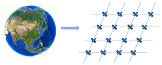
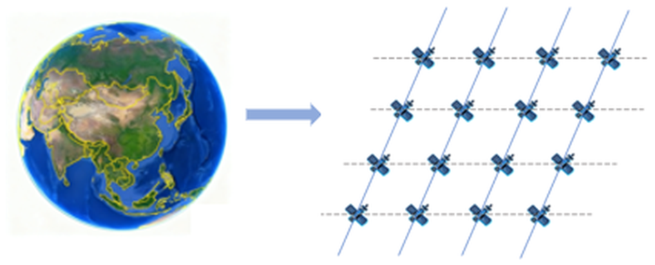
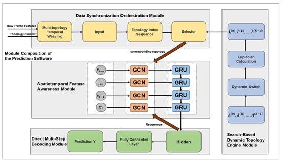
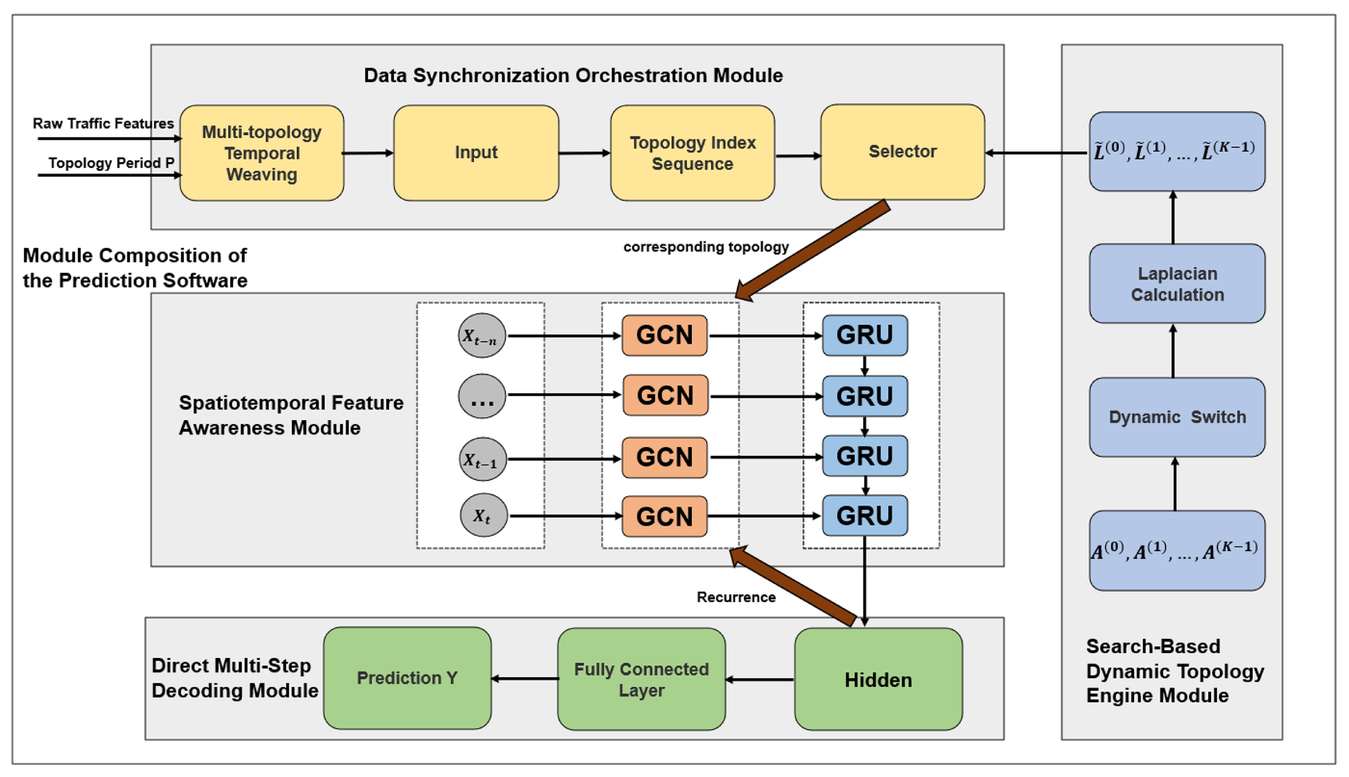
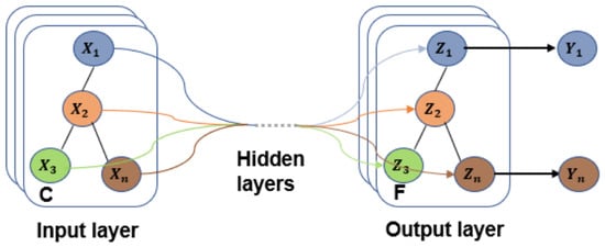
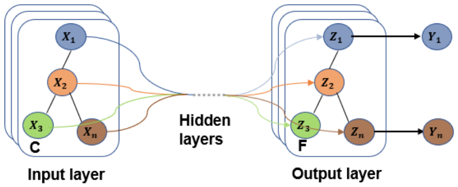
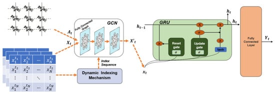
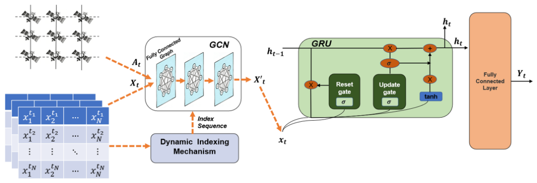
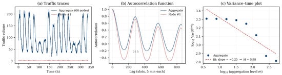
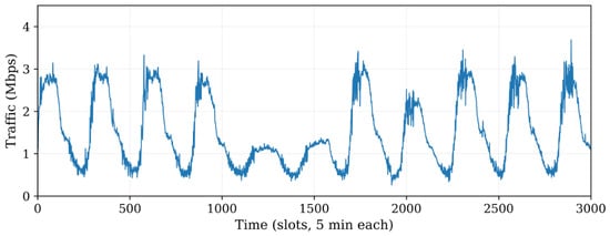
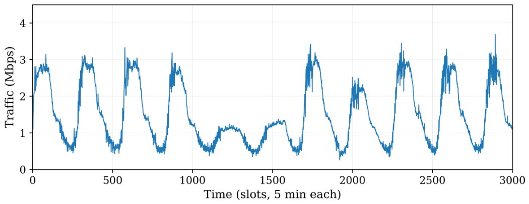
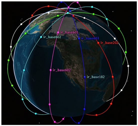
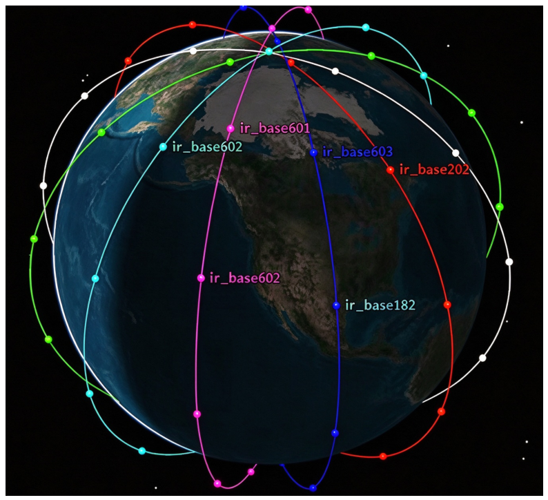
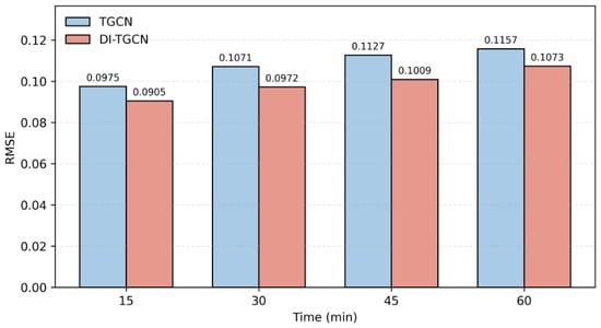
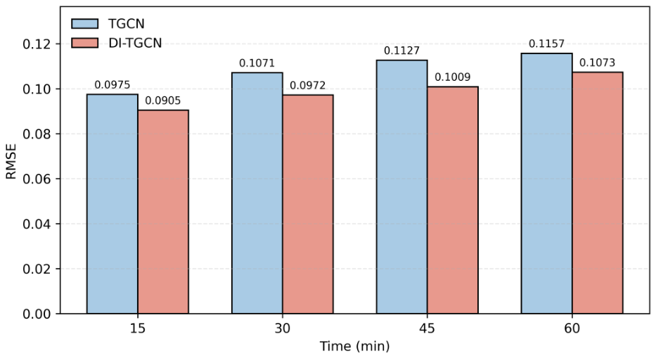
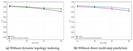
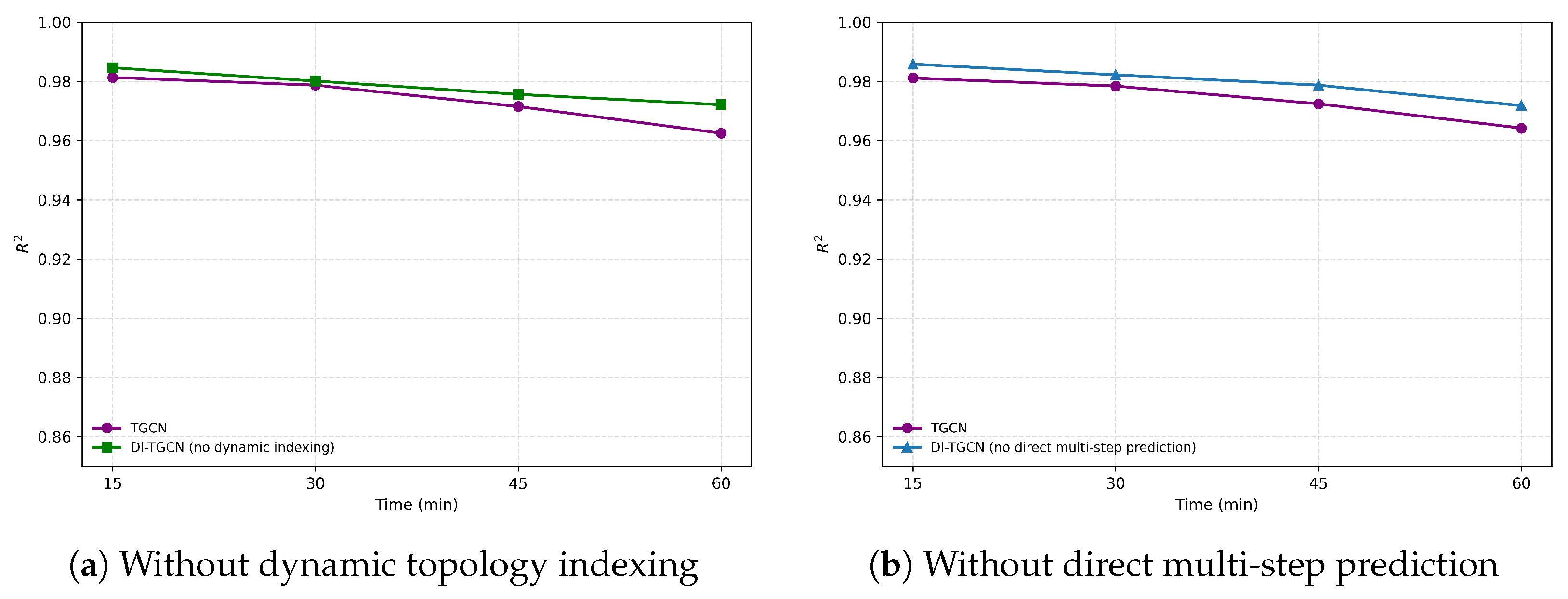
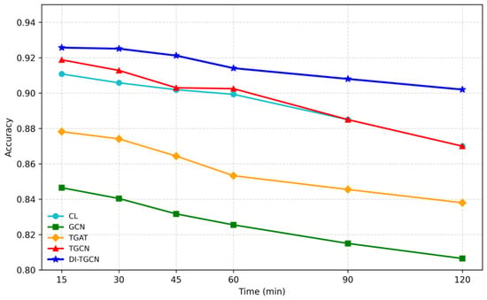
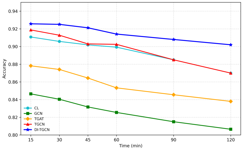
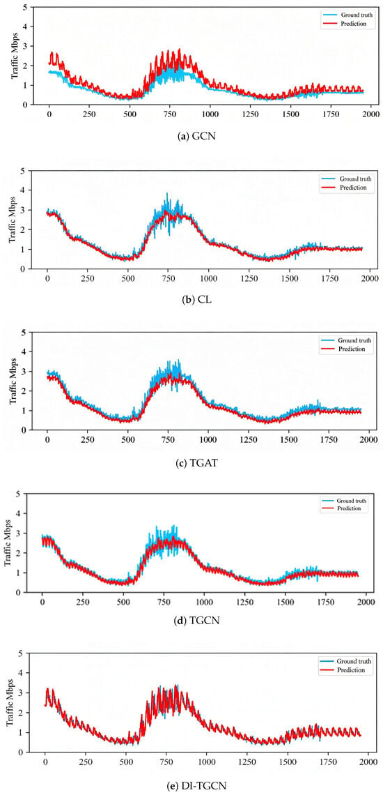
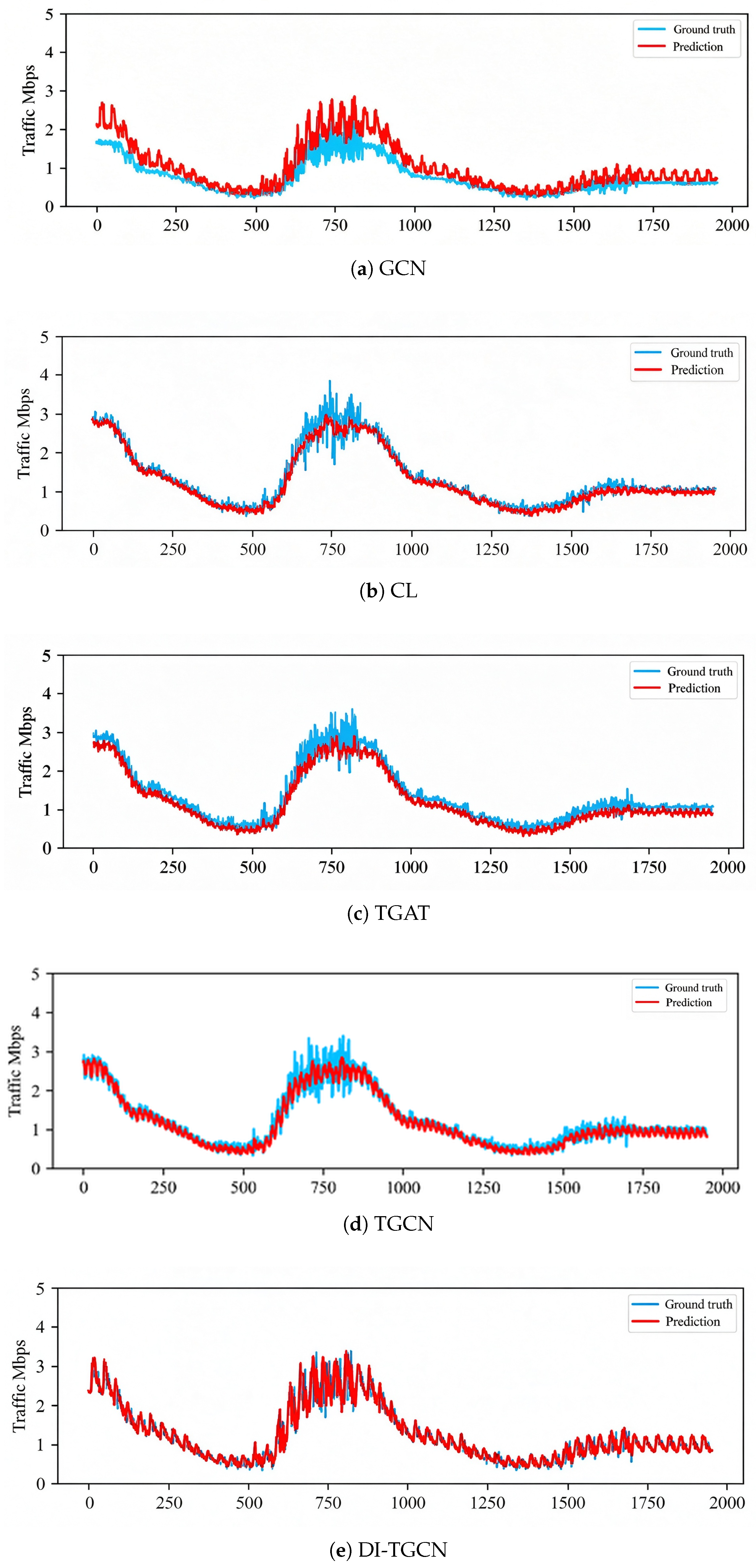
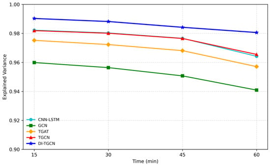
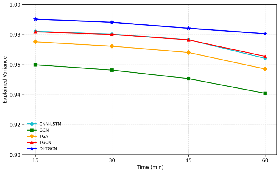
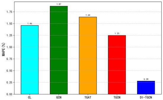
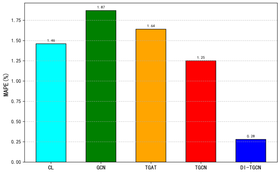
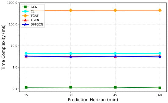
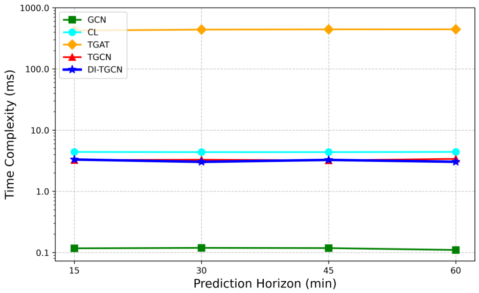

Disclaimer/Publisher’s Note: The statements, opinions and data contained in all publications are solely those of the individual author(s) and contributor(s) and not of MDPI and/or the editor(s). MDPI and/or the editor(s) disclaim responsibility for any injury to people or property resulting from any ideas, methods, instructions or products referred to in the content. |
© 2026 by the authors. Licensee MDPI, Basel, Switzerland. This article is an open access article distributed under the terms and conditions of the Creative Commons Attribution (CC BY) license.