Precision Measurement Method for Inertial Principal Axis Inclination of Aerospace Vehicles

Abstract

Inclination of the inertial principal axis in high-speed rotating rotors, spin-stabilized spacecraft, and other equipment induces dynamic unbalance and attitude–inertia coupling. Traceability and calibration technologies for principal axis inclination are critical to guarantee the dynamic performance of such equipment, yet a complete metrological calibration system remains absent. Aiming at the inherent model bias of the ellipsoid simplification algorithm widely adopted in engineering, this paper derives two sets of sufficient conditions—single-plane decoupling and transverse isotropy—under which the ellipsoid method and the 3D eigenvector method produce strictly identical, error-free results. Based on first-order eigenperturbation theory, an explicit bias scaling law is established: under general orientations, the model bias grows linearly with the inherent asymmetry of the rigid body and approximately linearly with the principal axis inclination, degenerating into a cubic function of inclination only under symmetric configurations; the first-order law is verified to remain quantitatively valid over the inclination range of 0–7°. Targeting zero theoretical error, a single-plane dual-counterweight loading calibration scheme is proposed; the mass centroid of the rigid body remains unchanged after loading, and three gradient calibration points of 2.0013°, 3.7869°, and 6.7970° are generated, fully covering the 0–7° engineering range with accurately traceable reference inclination angles. Three approaches—GUM, eigenperturbation, and Monte Carlo—are combined to evaluate the measurement uncertainty, and the expanded uncertainty of inclination at the calibration points with a coverage factor of 2 reaches 0.063°, with consistency among the three methods better than 0.12%. This work improves the error theory for inertial principal axis inclination measurement, and provides comprehensive theoretical support and simulation verification for traceability and calibration of this parameter.

1. Introduction

Mass characteristic parameters of a rigid body cover four core indicators: mass, centroid position, moment of inertia, and inertial principal axes. Up to now, two national metrological documents have been released in China: JJF 2030–2023 Calibration Specification for Centroid Measuring Instruments Using Multi-Point Weighing Method [1] and JJF 2329-2025 Calibration Specification for Moment of Inertia Measuring Instruments [2]. Mature measurement and traceability systems have been established for centroid and moment of inertia, while supporting calibration methods and quantity transfer schemes for inertial principal axis inclination are still lacking, forming an obvious gap in relevant metrology technologies. Internationally, analogous metrological documents have also been issued, such as the Guide to the Expression of Uncertainty in Measurement (JCGM 100:2008) [3], the NIST Technical Note 1297 guidelines for evaluating and expressing measurement uncertainty in the United States [4], and the Russian state standard GOST 8.207-76 for processing the results of direct measurements with multiple observations [5]; however, none of these documents provides a dedicated traceability scheme for inertial principal axis inclination either.

For high-speed rotating equipment such as aero-engine rotors, precision centrifuges, and spin-stabilized spacecraft, tilt of the inertial principal axis relative to the rotor rotation axis will trigger persistent dynamic unbalance and inertia coupling disturbance, directly degrading the dynamic stability and attitude control accuracy of the equipment. Accumulated mass eccentricity during multi-stage rotor assembly further amplifies principal axis deflection. Therefore, precise calculation, measurement, traceability, and calibration of principal axis inclination carry significant engineering value.

Principal axis inclination cannot be measured directly; it is solved by inverting the complete inertia tensor through multi-attitude moment-of-inertia tests. Two mainstream solution frameworks exist: the 3D eigenvector method and the 2D simplified ellipsoid method. The 3D eigenvector method yields strictly accurate results for arbitrary inertia tensors, yet the tensor components and principal axis inclination form an implicit function relationship, hindering analytical uncertainty propagation derivation. For simplified computation and convenient error sensitivity analysis, the 2D closed-form diagonalization solution for the submatrix of the inertia ellipsoid (referred to as the ellipsoid method) is widely adopted in engineering. Featuring compact formulation and low computational cost, it is extensively applied in rotor inertia testing and spacecraft inertial parameter identification [6].

The analytical formula for 2D ellipsoid principal axis inclination was systematically presented in classic rigid-body mechanics textbooks. Beer et al. [6] fully derived the simplified analytical expression for principal axis inclination within the XOZ plane, which was merely treated as a plane mechanics simplification tool without discussing inherent truncation errors induced by cross-coupling of 3D tensors. Early studies on spacecraft inertial parameter identification directly adopted the 2D ellipsoid formula for rapid estimation of principal axis orientation, assuming that the simplified model is globally accurate. Only external random errors such as sensor noise and attitude sampling deviation were compensated for, completely ignoring systematic bias introduced by the algorithm itself [7,8]. Volosov et al. [9] proposed an iterative ellipsoid estimation algorithm for satellite inertia identification, which only optimized numerical iteration convergence without analyzing the mechanical difference between 2D simplification and the exact 3D solution. Tanygin et al. [7] identified inertia tensors via multi-attitude coasting maneuvers and solved principal axes entirely using 2D ellipsoid approximation, without defining the applicable angular range of the model. Research on triaxial celestial-body principal axis perturbation in celestial mechanics only focused on orbital attitude disturbance, rather than the error evolution law of the 2D ellipsoid simplification algorithm as a function of inclination and asymmetry.

Domestic literature on rotor dynamics and inertial parameter measurement universally adopts the closed-form ellipsoid formula to calculate principal axis inclination [8,10,11]. He Xiaoxia et al. [8] combined torsional pendulum measurement with the ellipsoid method to rapidly calculate rotor principal axis inclination, without addressing computational bias caused by 3D inertial coupling. Yang Keji et al. [10] built an integrated measurement system for rotor principal axis inclination, yet no matching traceability calibration system was developed. Zhao Jun et al. [11] identified principal axis orientation relying on dynamic balance tests, likewise neglecting systematic bias from ellipsoid simplification. A small number of studies recognized computational bias of the ellipsoid method under large-inclination conditions, only qualitatively demonstrating error growth with increasing inclination via limited numerical examples. No research has derived the internal bias generation mechanism from tensor orthogonal transformation and first-order eigenperturbation theory, nor quantitatively divided the engineering applicable threshold for first-order approximate theory [12]. Published literature has not rigorously and completely derived two independent sufficient conditions for perfect equivalence between the ellipsoid method and 3D eigenvector method, making it impossible to design calibration standard part configurations with zero model error, and lacking theoretical foundations to support metrological calibration [13]. Meanwhile, uncertainty evaluation for ellipsoid method measurements mostly relies solely on Monte Carlo numerical simulation [12,14], without a complete evaluation framework combining analytical GUM propagation, eigenperturbation analysis, and Monte Carlo cross-verification, which impedes transparent error traceability required by calibration specifications [15,16].

In summary, three core deficiencies exist in the existing research: (1) The two independent sufficient constraints for zero error between the ellipsoid simplified solution and eigenvector method have not been systematically clarified, prohibiting design of calibration standards with theoretically bias-free reference values. (2) Scaling theory based on matrix eigenperturbation is absent, failing to quantitatively describe how inherent asymmetry and principal axis inclination affect systematic error. (3) A multi-path cross-verifiable uncertainty evaluation framework adapted to the ellipsoid method is missing, with no matching traceable calibration scheme to support quantity transfer of principal axis inclination. Accordingly, the aim of this study is to establish a complete theoretical and metrological framework for the precision measurement of inertial principal axis inclination, comprising the zero-error equivalence conditions between the ellipsoid method and the 3D eigenvector method, a quantitative bias scaling law with a clearly delimited valid domain, a traceable differential calibration scheme with zero theoretical model error, and a multi-path cross-verified uncertainty evaluation framework.

Targeting the above limitations, this paper conducts comprehensive theoretical derivation and numerical simulation analysis. First, two sets of sufficient conditions for strict equivalence between the ellipsoid method and eigenvector method are deduced from tensor orthogonal transformation perspectives. Relying on first-order eigenperturbation theory, a scaling relation is established where bias varies linearly with inherent asymmetry and approximately linearly with principal axis inclination under general orientations. A single-plane skew-symmetric dual-counterweight traceability calibration scheme is designed subject to zero-model-error constraints. Three mutually verifiable uncertainty evaluation pathways—analytical GUM propagation, eigenperturbation analysis and Monte Carlo simulation—are constructed, complying with JJF 1059.1-2012 [17] and JJF 1059.2-2012 [18]. The outcomes of this paper provide complete theoretical and simulation evidence for compiling dedicated calibration specifications for inertial principal axis inclination and traceability of inertia parameters for rotating equipment [19,20].

2. Error Mechanism of the Inertial Principal Axis Ellipsoid Inclination Model

2.1. Measurement Model for Inertial Principal Axis Ellipsoid Inclination

The inertial principal axis is an inherent property of a rigid body, defined by the central inertia tensor passing through the centroid. In practical measurement, mass characteristic measuring instruments first determine the centroid position [1,21,22], then convert the measured moments of inertia at each attitude into the centroidal central tensor via the parallel axis theorem. All inertia tensors and principal axis inclinations discussed in this paper refer to such centroidal central tensors. Let the real symmetric centroidal inertia tensor of the rigid body in coordinate system OXYZ (origin at centroid, z-axis aligned with vertical/assembly geometric reference) be expressed as Equation (1) [23]:

$$I=\left[\begin{array}{ccc}{I}_{\mathit{xx}}& -I_{\mathit{xy}}& -I_{\mathit{xz}}\\ -I_{\mathit{xy}}& I_{\mathit{yy}}& -I_{\mathit{yz}}\\ -I_{\mathit{xz}}& -I_{\mathit{yz}}& I_{\mathit{zz}}\end{array}\right]$$

(1)

where I_xx, I_yy, and I_zz denote moments of inertia, and I_xy, I_yz, and I_xz denote products of inertia. The eigenvectors of I correspond to principal axis orientations.

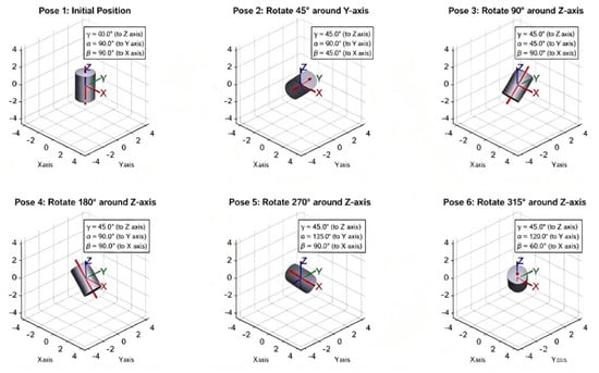
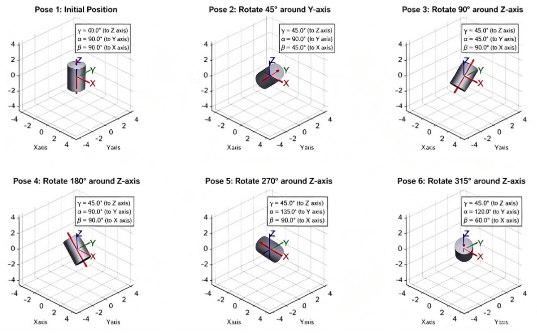
As illustrated in Figure 1, the multi-attitude measurement method is commonly adopted in engineering to acquire the complete inertia tensor [4,5]: the test piece is fixed on a torsional pendulum table at distinct spatial attitudes, and the moment of inertia about the rotation axis is measured sequentially. The measured value at each attitude satisfies $J_k=n_k^T\cdot I\cdot n_k$, where n_k represents the unit direction vector of the pendulum rotation axis at the i-th attitude. When no fewer than six attitudes are measured, an overdetermined system of equations can be constructed to invert all six independent tensor components, as shown in Equation (2):

$$J_i=I_{\mathit{xx}}{l}_i^2+I_{\mathit{yy}}{m}_i^2+I_{\mathit{zz}}{n}_i^2-2I_{\mathit{xy}}{l}_i{m}_i-2I_{\mathit{yz}}{m}_i{n}_i-2I_{\mathit{xz}}{l}_i{n}_i$$

(2)

where l_i, m_i, n_i respectively represent the direction cosines between the X, Y, and Z axes of the centroid coordinate system and the pendulum rotation axis at the i-th attitude.

Figure 1. Schematic of inertial principal axis inclination measurement using six typical attitudes in the measurement coordinate system.

For the measured inertia tensor, the inclination angle θ_z between the z-direction inertial principal axis and the geometric z-axis can be calculated via two approaches. The eigenvector method extracts the eigenvector corresponding to the maximum principal moment of inertia and substitutes it to solve for inclination; this method holds strictly for arbitrary I and serves as the calculation benchmark of this paper. However, eigenvector components and inertia tensor elements form an implicit function, complicating analytical uncertainty propagation. The ellipsoid method separately diagonalizes the 2 × 2 submatrices within the XOZ and YOZ planes to obtain compact analytical expressions, as systematically presented in classic rigid-body mechanics textbooks [3] and shown in Equation (3):

$$\left\{\begin{array}{l}{\phi }_{\mathit{zy}}={\displaystyle \frac{1}{2}}\arctan {\displaystyle \frac{2I_{\mathit{yz}}}{I_{\mathit{zz}}-I_{\mathit{yy}}}}\\ {\phi }_{\mathit{zx}}={\displaystyle \frac{1}{2}}\arctan {\displaystyle \frac{2I_{\mathit{xz}}}{I_{\mathit{xx}}-I_{\mathit{zz}}}}\\ {\theta }_z^{2D}=\arctan \sqrt{{\tan }^2{\phi }_{\mathit{zx}}+{\tan }^2{\phi }_{\mathit{zy}}}\end{array}\right.$$

(3)

The 2D analytical inclination Formula (3) only utilizes tensor components within the XOZ and YOZ subplanes, featuring closed-form mathematical formulation that facilitates error sensitivity analysis and uncertainty propagation computation. Nevertheless, this simplified model discards cross-plane coupling terms inherent to the 3D inertia tensor, and yields results completely equivalent to the 3D eigenvector method only under specific tensor constraint conditions. If the test rigid body fails to satisfy equivalence prerequisites, systematic model bias will be introduced by the 2D simplification. Accordingly, the following sections focus on deriving sufficient conditions for perfect equivalence between the ellipsoid closed-form solution and eigenvector method, revealing the generation mechanism of model bias, and analyzing the quantitative applicable range of the simplified model via perturbation theory and numerical simulation.

The intrinsic distinction between the two approaches can be stated both algebraically and geometrically. Algebraically, the ellipsoid method solves the eigenvalue problem of the 2 × 2 principal submatrices extracted from the full inertia tensor, which is equivalent to forcibly setting the cross-plane coupling terms to zero, whereas the 3D eigenvector method diagonalizes the complete tensor in which all coupling terms participate simultaneously. Geometrically, the ellipsoid method measures the axis tilt of the ellipses obtained by projecting the 3D inertia ellipsoid onto the XOZ and YOZ coordinate planes, while the eigenvector method directly determines the axes of the 3D ellipsoid itself. The axes of the projected ellipses coincide with the true ellipsoid axes only when the projected sections are principal sections of the tensor, which is precisely the geometric meaning of the two sufficient conditions derived in Section 2.2.

2.2. Scaling Law and Valid Applicable Threshold of Ellipsoid Model Bias

Let the inherent inertia tensor of the rigid body in the principal axis coordinate system be I_p, transformed into the observed tensor I via rotation matrix R. Equation (2) and the eigenvector method yield consistent results under two mutually independent sufficient conditions. Define bias as $\Delta \theta ={\theta }_z^{(2D)}-{\theta }_z$; the paper derives the necessary and sufficient conditions for Δθ = 0 and corresponding scaling laws. Throughout this paper, a parenthesized superscript on the inclination symbol distinguishes the solution method: the superscript (E) denotes the result of the 2D ellipsoid closed-form formula, while the superscript (3D) denotes the exact result of the 3D eigenvector method; the superscripts are omitted in Equation (3) and elsewhere where no ambiguity arises.

Sufficient Condition 1: Single-plane decoupling

If all elements in the y-row and y-column of the inertia tensor vanish except diagonal terms (I_xy = I_yz = 0), the tensor simplifies to:

$$I=\left[\begin{array}{ccc}{I}_{\mathit{xx}}& 0& -I_{\mathit{xz}}\\ 0& I_{\mathit{yy}}& 0\\ -I_{\mathit{zx}}& 0& I_{\mathit{zz}}\end{array}\right]$$

(4)

Expanding the characteristic equation along the second row yields two categories of eigenvalues: (1) When solving for the eigenvector associated with I_yy, the y-axis is naturally a principal axis. (2) The remaining two eigenvalues satisfy the characteristic equation of the xoz 2D submatrix, whose diagonalization rotation angle equals the inclination solved by Equation (3). Under this condition, Δθ = 0 strictly holds, meaning that the 3D eigenvector method and 2D ellipsoid closed-form solution produce identical principal axis inclination results, regardless of rotational symmetry of the rigid body.

Sufficient Condition 2: Transverse isotropy

Assume that the principal axis tensor satisfies transverse isotropy ($I_{\mathit{xx}}^{\prime }=I_{\mathit{yy}}^{\prime }\triangleq I_{\perp },I_{\mathit{zz}}^{\prime }=I_{\parallel }$), i.e., the rigid body features rotational symmetry about the z-direction principal axis. Arbitrary orthogonal rotation can be decomposed into azimuth rotation and pitch tilt. With rotation matrix simplified to pure pitch tilt as Equation (5):

$$R=\left[\begin{array}{ccc}\cos \mathit{\theta }& 0& \sin \mathit{\theta }\\ 0& 1& 0\\ -\sin \mathit{\theta }& 0& \cos \mathit{\theta }\end{array}\right]$$

(5)

The observed inertia tensor is derived as Equation (6):

$$I=R_{\theta }^T{I}^{\prime }{R}_{\theta }=\left[\begin{array}{ccc}{I}_{\perp }{\cos }^2\theta & 0& (I_{\perp }-I_{\parallel })\cos \mathit{\theta }\sin \mathit{\theta }\\ 0& I_{\perp }& 0\\ (I_{\perp }-I_{\parallel })\cos \mathit{\theta }\sin \mathit{\theta }& 0& I_{\parallel }\end{array}\right]$$

(6)

Transverse isotropy inherently satisfies Condition 1 (I_xy = I_yz = 0), so Equation (3) yields strictly accurate inclination with zero bias.

For combined azimuth and pitch tilt, rotational symmetry guarantees I_xy = I_yz, I_yz = I_xztanϕ (Equation (7)). Substituting into the ellipsoid rotation angle formula gives Equation (8). Rigorous proof via tensor orthogonal transformation confirms Δθ = 0: as long as the rigid body possesses inherent transverse isotropy, the ellipsoid closed-form solution remains bias-free under arbitrary 3D tilt orientations.

$$I=R_{\varphi }^T{R}_{\theta }^T{I}^{\prime }{R}_{\theta }{R}_{\varphi }=\left[\begin{array}{ccc}(I_{\perp }{\cos }^2\theta +I_{\parallel }{\sin }^2\theta ){\cos }^2\varphi +I_{\perp }{\sin }^2\varphi & -(I_{\perp }-I_{\parallel })\cos \mathit{\beta }\sin \mathit{\beta }\sin \mathit{\varphi }\cos \mathit{\varphi }& -(I_{\perp }-I_{\parallel })\cos \mathit{\theta }\sin \mathit{\theta }\cos \mathit{\varphi }\\ -(I_{\perp }-I_{\parallel })\cos \mathit{\theta }\sin \mathit{\theta }\sin \mathit{\varphi }\cos \mathit{\varphi }& I_{\perp }{\cos }^2\beta +I_{\parallel }{\sin }^2\beta ){\sin }^2\varphi +I_{\perp }{\cos }^2\varphi & (I_{\perp }-I_{\parallel })\cos \mathit{\theta }\sin \mathit{\theta }\sin \mathit{\varphi }\\ -(I_{\perp }-I_{\parallel })\cos \mathit{\theta }\sin \mathit{\theta }\cos \mathit{\varphi }& (I_{\perp }-I_{\parallel })\cos \mathit{\beta }\sin \mathit{\theta }\sin \mathit{\varphi }& I_{\perp }{\sin }^2\theta +I_{\parallel }{\cos }^2\theta \end{array}\right]$$

(7)

Equation (7) indicates that both I_xy and I_yz are non-zero, yet rotational symmetry yields I_yz = I_xztanϕ. Substituting this relation into the rotation angle formula of the ellipsoid method produces Equation (8):

$$\left\{\begin{array}{l}{\phi }_{\mathit{zy}}={\displaystyle \frac{1}{2}}\arctan {\displaystyle \frac{2I_{\mathit{yz}}}{I_{\mathit{zz}}-I_{\mathit{yy}}}}\\ {\phi }_{\mathit{zx}}={\displaystyle \frac{1}{2}}\arctan {\displaystyle \frac{2I_{\mathit{xz}}}{I_{\mathit{xx}}-I_{\mathit{zz}}}}\end{array}\right.$$

(8)

The omitted intermediate steps are supplemented as follows. Expanding the orthogonal transformation of the inertia tensor element-wise under transverse isotropy shows that the azimuth-dependent factors separate from the tilt-dependent factors: the two cross-plane products of inertia share a common amplitude proportional to the product of the axial-transverse inertia difference and the sine–cosine product of the inclination, modulated respectively by the cosine and sine of the tilt azimuth. Substituting the two components into the planar closed-form expressions of Equation (3), the azimuth factors cancel identically in each planar arctangent ratio, and both planar solutions return exactly the true inclination. This cancellation constitutes the logical link between Equations (7) and (8): rotational symmetry removes the azimuth dependence of the planar ratios, so the closed-form ellipsoid solution coincides with the true tilt under arbitrary 3D orientations.

Rigorous proof based on tensor orthogonal transformation verifies Equation (3): if a rigid body inherently satisfies transverse isotropy, the closed-form ellipsoid solution introduces zero bias for arbitrary three-dimensional tilt orientations, i.e., Δθ = 0.

$$\arctan \sqrt{{\tan }^2{\phi }_{\mathit{zx}}+{\tan }^2{\phi }_{\mathit{zy}}}=\arccos \left|v_z\right|$$

(9)

In Equation (9), ν_z denotes the z-component of the unit eigenvector corresponding to the maximum principal moment of inertia, which equals the cosine of the angle between the z-direction principal axis and the reference z-axis.

When the rigid body satisfies neither single-plane decoupling nor transverse isotropy, inherent systematic bias emerges between the 2D ellipsoid closed-form solution and exact 3D eigenvector results. The following section strictly derives the scaling law of bias as a function of inherent asymmetry and inclination based on first-order real symmetric matrix eigenperturbation theory.

Define the inherent inertia tensor of the rigid body in the principal axis coordinate system as Equation (10):

$$I^{\prime }=I_0^{\prime }+\delta \Delta I^{\prime }$$

(10)

where:

I^′ = diag(I_⊥,I_⊥,I_∥): Rotationally symmetric reference tensor satisfying transverse isotropy;

$\delta =\left|I_{\mathit{xx}}^{\prime }-I_{\mathit{yy}}^{\prime }\right|$: Inherent asymmetry of the rigid body, quantifying the deviation of the triaxial inertia ellipsoid from rotational symmetry;

ΔI^′ = diag(1/2, −1/2, 0): Unit asymmetry perturbation matrix.

The centroidal observed inertia tensor follows orthogonal transformation:

$$I=R^T{I}^{\prime }R=R^T(I_0^{\prime }+\delta \Delta I^{\prime })R=I_0+\delta \Delta I$$

(11)

Here, I = R^TI^′R denotes the observed tensor corresponding to the symmetric reference state (zero model bias, unperturbed principal axis inclination), while δΔI represents the tensor perturbation introduced by asymmetry, which shifts principal axis eigenvectors and generates inclination bias.

Eigenvalues and eigenvectors satisfy I₀v₀ = λ₀v₀ under unperturbed conditions. Introducing infinitesimal tensor perturbation δΔI, eigenvalues and eigenvectors shift slightly to v = v₀ + Δv, λ = λ₀ + Δλ. Substitute into the characteristic equation to obtain Equation (12):

(I₀ + δΔI)(v₀ + Δv) = (λ₀ + Δλ)(v₀ + Δv)

(12)

In Equation (12), λ denotes an eigenvalue of the inertia tensor, i.e., the principal moment of inertia associated with the corresponding eigenvector, and the perturbed eigenpairs are expanded to first order in the asymmetry perturbation.

Project perturbed eigenquantities onto other orthogonal eigenvectors using the completeness of orthogonal principal axis bases to solve for δλ, δν. Axial principal axis inclination is defined as the angle between the reference z-axis and the principal axis eigenvector θ = arccos|v₂|, yielding the differential transfer relation between inclination and the z-component of eigenvectors (Equation (13)):

$$\mathit{d\theta }=-{\displaystyle \frac{1}{\sqrt{1-v_z^2}}}d{v}_z$$

(13)

Perturbed principal axis inclination reads θ = θ₀ + Δθ, where v_z = v_0z + Δv_z denotes the corresponding eigenvector. Under weak asymmetry and small-inclination conditions, bias satisfies the linear approximation in Equation (14):

Δθ∝|Δv_z|

(14)

When neither of the two sufficient conditions is satisfied, the magnitude of the bias can be analyzed using the first-order eigenperturbation theory for real symmetric matrices. Let $\delta =\left|I_{\mathit{xx}}^{\prime }-{I^{\prime }}_{\mathit{yy}}\right|$, ϕ the tilt azimuth, ψ the spin angle, and ΔI the difference between axial and transverse moments of inertia. For general three-dimensional orientations, the leading-order bias of the closed-form solution is expressed as Equation (15):

$$\left|{\theta }_z^{2D}-{\theta }_z\right|\approx \mathit{\kappa \delta }{\theta }_z,\kappa ={\displaystyle \frac{\sin 2\mathit{\varphi }\sin 2\left(\varphi +\psi \right)}{2\left(I_{\perp }-I_{\parallel }\right)}}$$

(15)

That is, the bias grows linearly with the inherent asymmetry δ and the principal axis inclination θ_z, and is amplified as the axial-transverse inertia difference decreases. The first-order terms cancel out only when the tilt azimuth is aligned with or orthogonal to the transverse principal inertia axes (sin2ϕ = 0 or sin2(ϕ + φ) = 0, e.g., single-plane loading and symmetric bidirectional tilting), where the bias degenerates into a cubic function of the inclination angle. When δ = 0 (rotational symmetry), κ = 0, and the bias equals zero strictly.

With a fixed principal axis inclination θ_z, the computational bias of the ellipsoid method is linearly proportional to the inherent asymmetry δ of the rigid body. With a fixed inherent asymmetry δ, the bias rises linearly with the principal axis inclination (reducing to a cubic relationship for symmetric configurations), and the amplification effect of model error becomes more prominent at larger inclination angles. If the rigid body is fully rotationally symmetric (δ = 0), Δθ = 0 holds for any inclination magnitude; the closed-form ellipsoid solution is strictly equivalent to the three-dimensional eigenvector method, with no direct correlation to the cross terms I_xy, I_yz, I_xz of the observed inertia tensor.

The bias scaling law derived from first-order eigenperturbation and presented in Equation (15) demonstrates that the model bias of the ellipsoid method bears a linear correlation with the rigid body’s inherent asymmetry and grows linearly with the principal axis inclination. This analytical expression is established on the premise of first-order linear approximation under weak asymmetry and small inclination, and can only be used for quantitative calculation when the relative error induced by truncated high-order infinitesimal terms falls within engineering allowable limits. As the principal axis inclination and asymmetry continuously increase, high-order terms become non-negligible, and the first-order scaling approximation will deviate drastically from the true model bias, losing its capacity for quantitative prediction. Accordingly, it is necessary to quantitatively define the valid inclination threshold of the scaling law and clarify the applicable boundary of the first-order approximate model.

To quantitatively delimit this valid domain, a two-dimensional numerical sweep over the inherent asymmetry (0.5 ≤ δ ≤ 10) and the principal axis inclination (0° ≤ θz ≤ 10°) was carried out, comparing the first-order prediction of Equation (15) with the exact bias computed by the 3D eigenvector method. The relative deviation of the first-order scaling law remains below 1% within δ ≤ 1 and θz ≤ 7°, and grows rapidly beyond this range as cubic and higher-order terms accumulate. The engineering range of 0~7° adopted in this paper therefore lies well inside the valid domain of the first-order perturbation approximation, within which the residual truncation error of the scaling law is more than one order of magnitude smaller than the measurement uncertainty evaluated in Section 4.

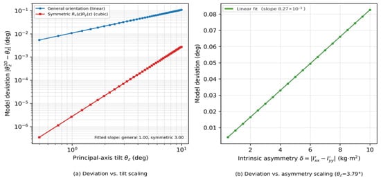
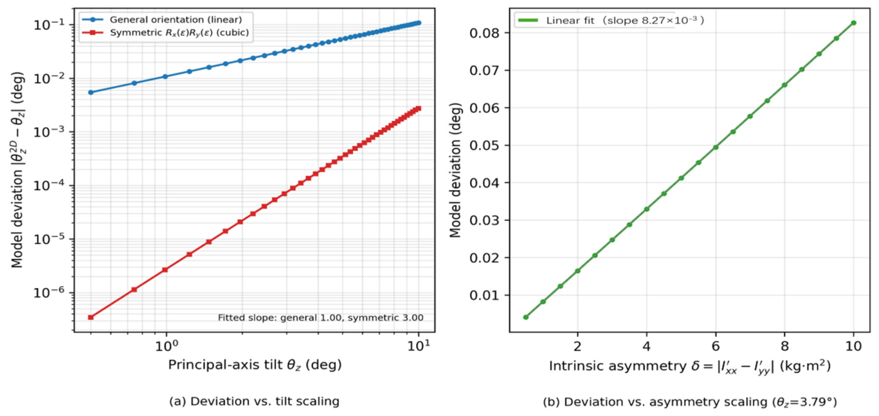
Simulation results from Figure 2 and Table 1 further verify the derived ellipsoid bias scaling law. Under general orientations, bias nearly doubles as inclination doubles (blue curve in Figure 2a, slope ≈ 1), presenting linear growth. For symmetric bidirectional tilt configurations (red curve, slope ≈ 3), bias degenerates to a cubic function of inclination, arising from azimuth–spin coupling factors approaching zero along this specific path. Controlled experiments at fixed inclination 3.79° with varying asymmetry confirm linear correlation between bias and δ (Figure 2b). When δ = 0 (rigid body satisfies rotational symmetry), computational bias remains at the 10⁻¹³ magnitude regardless of inclination, proving that inherent asymmetry is the sole root cause of systematic bias in the ellipsoid simplification model. It should be clarified that all experiments referred to in this section are numerical simulation experiments: synthetic inertia tensors with prescribed inherent asymmetry and principal axis inclination are generated numerically, and the bias is obtained by comparing the ellipsoid closed-form solution with the 3D eigenvector benchmark; no physical test is involved at this stage.

Figure 2. Mechanism of closed-form ellipsoid solution bias. (a) Bias grows linearly with inclination under general orientations (cubic dependence for symmetric configurations); (b) bias increases linearly with asymmetry at fixed inclination.

Table 1. Analysis of influencing factors for ellipsoid closed-form solution bias.

Numerical Test Case	Bias/°	Conclusion
Symmetric specimen (δ = 0), bidirectional tilt, non-zero Ixy	~10−13	Exact solution at δ = 0, independent of Ixy
Fixed δ = 5, inclination increased from 1° to 8°	8 × 10−6 → 4 × 10−3	Bias proportional to inclination (cubic for symmetric configurations)
Fixed inclination 3°, δ increased from 1 to 10	4 × 10−5 → 3 × 10−4	Bias proportional to asymmetry δ

3. Traceability Calibration Scheme for Inertial Principal Axis Inclination Based on Zero-Model-Error Conditions

As derived in Section 2.2, the 2D ellipsoid closed-form solution yields principal axis inclination completely consistent with the 3D eigenvector method without systematic bias if the rigid body satisfies either single-plane decoupling (I_xy = I_yz = 0) or transverse isotropy ($I_{\mathit{xx}}^{\prime }=I_{\mathit{yy}}^{\prime }$). Taking these two zero-error constraints as theoretical foundations, a traceable calibration system with perfectly accurate theoretical reference inclination values can be constructed.

Targeting the industry-wide lack of dedicated traceability calibration methods for inertial principal axis inclination, this paper establishes three theoretically feasible calibration schemes centered on zero theoretical model error, quantity traceability, and cancelable common-mode systematic error, based on the two zero-error constraints. Comprehensive comparisons are conducted across dimensions including metrological traceability difficulty, fixture manufacturing cost, on-site operational complexity, and additional uncertainty from reassembly, identifying the single-plane dual-counterweight loading scheme as the primary calibration solution.

3.1. Principle and Workflow of Differential Comparison Calibration

The calibration logic adopted in this paper aligns with the shift-axis differential calibration method specified in JJF 2329-2025, Calibration Specification for Moment of Inertia Measuring Instruments [2]. Measured inclination differences between two tests are taken as instrument indication error, effectively canceling common-mode systematic errors that cannot be fully eliminated, such as residual baseline inclination of standard parts, unlevel test fixtures, and fixed eccentricity of torsional pendulum tables, drastically reducing systematic uncertainty of calibration results.

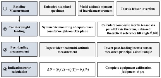
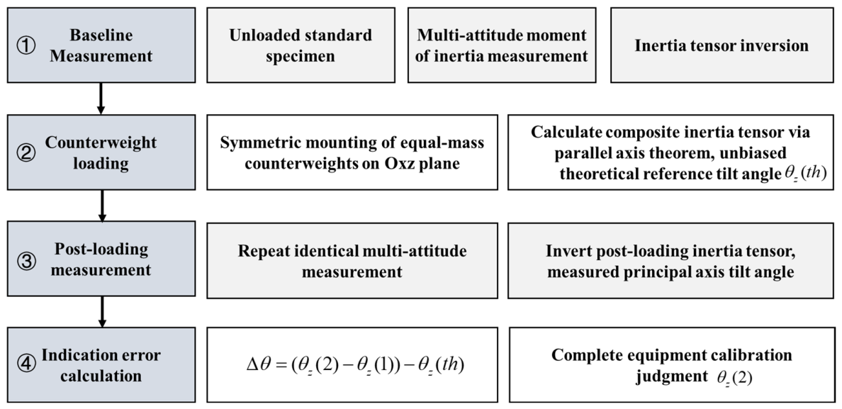
The complete calibration workflow is divided into four core phases: baseline measurement, counterweight loading, post-loading remeasurement, and indication error calculation, as illustrated in Figure 3.

Figure 3. Complete workflow of differential comparison calibration for inertial principal axis inclination.

Baseline Measurement: Mount the unloaded rotationally symmetric standard part firmly on the torsional pendulum test fixture. Collect multiple groups of moment-of-inertia data across six attitudes, invert the full centroidal inertia tensor via multi-attitude overdetermined equations, and solve the unloaded baseline principal axis inclination via 3D eigenvector decomposition. This step captures common-mode systematic errors including fixture installation tilt and residual inherent offset of standard parts as cancellation benchmarks for subsequent steps.

Counterweight Loading: Symmetrically install equal-mass counterweights within the xoz coordinate plane. Calculate the inertia tensor increment introduced by counterweights via the parallel axis theorem, and derive bias-free theoretical reference inclination combined with baseline inertial parameters of the standard part. This theoretical value is traceable solely to mass and length metrological benchmarks [20], free of systematic model bias from ellipsoid simplification.

Post-Loading Remeasurement: Retain identical fixture mounting, standard part attitude, and all measurement attitudes after counterweight assembly. Repeat moment-of-inertia acquisition and tensor inversion to obtain measured principal axis inclination under loaded conditions. Consistent measurement layout eliminates additional uncertainty induced by attitude differences and guarantees identical error sources for both measurements.

Indication Error Calculation: Substitute into the indication error formula to quantitatively evaluate instrument metrological performance. The inclination difference between two measurements cancels fixed baseline deviation, realizing quantitative calibration of inertial principal axis inclination measuring equipment. In the indication error formula, θ(1) denotes the measured principal axis inclination of the unloaded standard part obtained in the baseline phase, and θ(2) denotes the measured inclination after counterweight loading; the difference between the two measurements cancels the common-mode baseline deviation.

3.2. Single-Plane Dual-Counterweight Calibration Scheme Satisfying Single-Plane Decoupling

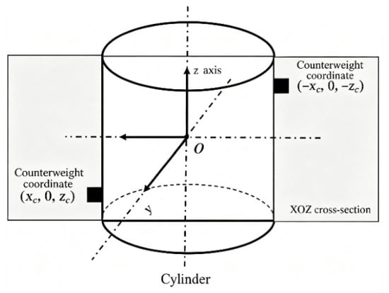
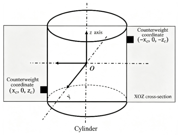
Shown as Figure 4, to generate theoretically bias-free, traceable reference inclination values, a homogeneous solid cylinder is selected as the calibration reference standard part. Naturally featuring transverse isotropy under unloaded conditions, its inertial principal axis fully coincides with the geometric z-axis, yielding a theoretical baseline inclination of zero without counterweights. The standard part is uniformly designed with radius r = 0.5 m, height h = 2 m, and total mass 500 kg. Baseline moments of inertia are solved via rigid-body centroidal inertia formulas in Equation (16), with zero cross products of inertia and no 3D inertial coupling effects.

$$\left\{\begin{array}{l}{I}_{\mathit{xx}}^{\prime }=I_{\mathit{yy}}^{\prime }={\displaystyle \frac{1}{12}}m(3r^2+h^2)=197.92\mathrm{kg}\cdot {\mathrm{m}}^2\\ I_{\mathit{zz}}^{\prime }={\displaystyle \frac{1}{2}}m{r}^2=62.50\mathrm{kg}\cdot {\mathrm{m}}^2\end{array}\right.$$

(16)

Figure 4. Geometric schematic of standard part and counterweight blocks.

All counterweights are arranged exclusively within the xoz plane with symmetric coordinates (x_c,z_c) and (−x_c,−z_c); fixed installation dimensions are set as x_c = 0.5 m, z_c = 1.0 m. This layout delivers two core metrological advantages: (1) The first moment vectors of the two counterweights relative to the centroid cancel each other out, so the centroid position of the composite rigid body remains unchanged before and after loading. (2) The y-coordinate of all counterweights equals zero, enforcing I_xy = I_yz = 0 and strictly satisfying the single-plane decoupling zero-error condition derived in Section 2.2. The difference between ellipsoid closed-form inclination and 3D eigenvector results falls below 10⁻¹³, eliminating inherent systematic model bias. Here, m denotes the total mass of the standard part, and m₀ denotes the mass of each individual counterweight.

The inertia tensor increment introduced by counterweights is expressed via the parallel axis theorem as Equation (17). Substituting fixed installation dimensions simplifies the composite inertia components to I_xx = 197.92 + 2m₀, I_zz = 62.50 + 0.5m₀, I_xz = m₀. Substituting components into the ellipsoid inclination solving formula yields corresponding theoretical reference inclination. Although I_xx ≠ I_yy after loading, the xoz 2D submatrix is independent of I_yy; variations in I_yy only affect yoz plane calculation without disturbing inclination solving accuracy for this single-plane scheme. Thus, the standard part does not require perfectly rotationally symmetric cross-sections, significantly lowering manufacturing difficulty. Explicitly, the composite inertia components after loading are Ixx = 197.92 + 2m₀z_c², Izz = 62.5 + 2m₀x_c², and Ixz = −2m₀x_cz_c (all in kg·m², with m₀ in kg and the installation dimensions x_c, z_c in m), so that every term is dimensionally consistent; substituting x_c = 0.5 m and z_c = 1.0 m yields the simplified numerical coefficients shown above.

$$\left\{\begin{array}{l}\Delta I_{\mathit{xx}}=2m_0{z}_c^2\\ \Delta I_{\mathit{yy}}=2m_0\left(x_c^2+z_c^2\right)\\ \Delta I_{\mathit{zz}}=2m_0{x}_c^2\\ \Delta I_{\mathit{xz}}=2m_0{x}_c{z}_c\end{array}\right.$$

(17)

Three groups of counterweights (5 kg, 10 kg, 20 kg) are selected to construct three gradient calibration points, with selection rationales layered as follows: (1) Engineering range matching: Principal axis tilt after assembly for aerospace rotors, centrifuges, and spacecraft cabins mostly falls within the 0–7° range. The three counterweight groups correspond to theoretical inclinations 2.0013°, 3.7869°, and 6.7970°, fully covering the conventional industrial detection range. (2) Metrological graded calibration demand: Small, medium, and large gradient points support zero-point verification for low measurement range, linear error evaluation for medium range, and limit precision testing for high range, respectively, fully satisfying multi−point segmented calibration workflows required by metrological specifications.

Practical implementation factors of the loading scheme are further analyzed as follows, as illustrated in Table 2. (1) Counterweight mounting precision: taking the medium calibration point (10 kg counterweights) as an example, sensitivity analysis of the theoretical reference inclination shows that a ±0.5 mm deviation of the axial installation dimension z_c changes the reference inclination by about 0.001°, a ±0.5 mm deviation of the radial dimension x_c by about 0.002°, and a counterweight mass deviation of ±10 g by about 0.002°; all of these contributions remain below 4% of the expanded uncertainty (0.063°) and are already incorporated into the uncertainty budget of Section 4 through the counterweight mass and positioning uncertainty terms. (2) Repeatability of disassembly and reassembly: the differential scheme retains identical fixture mounting and measurement attitudes in the two measurement phases, so reassembly alignment deviations enter both measurements as common-mode errors and cancel in the indication error. (3) Machining tolerances of the standard part and fixtures: as analyzed above, the reference inclination of this scheme is independent of Iyy, hence moderate deviation of the cylinder cross-section from perfect rotational symmetry does not disturb the theoretical reference value. Moreover, residual antisymmetric misplacement of the counterweights breaks the exact centroid preservation only to a limited extent: for a ±0.5 mm antisymmetric misplacement, the residual centroid shift of the 520 kg composite body is below 0.02 mm, and its effect on the reference inclination is negligible compared with the uncertainty budget.

Table 2. Selection of three gradient inclination calibration points.

Calibration Point	Counterweight Mass m0/kg	Product of Inertia Ixz/(kg·m2)	Theoretical Inclination θz(th)/°
Small inclination point	5	5	2.0013
Medium inclination point	10	10	3.7869
Large inclination point	20	20	6.7970

4. Measurement Uncertainty Evaluation

Uncertainty Evaluation Framework

Uncertainty evaluation is conducted in compliance with JJF 1059.1-2012, JJF 1059.2-2012, and the GUM metrology guide. The evaluation target is the principal axis inclination indication error output from the differential calibration scheme in Chapter 3. Mathematical relations including tensor inversion, inclination solving, and parallel axis transformation serve only as error transfer measurement models, not evaluation objects. The complete measurement model for indication error reads: Δθ = (θ_z(2) − θ_z(1)) − θ_z(th), where θ_z(1) denotes unloaded baseline inclination of the standard part, θ_z(2) measured inclination after counterweight loading, and θ_z(th) theoretical standard inclination introduced by counterweights. Error transfer splits into two chains: (1) Measured inclination: Derived from multi-attitude moments of inertia via tensor inversion and ellipsoid formula solving. (2) Standard theoretical inclination: Calculated from counterweight mass, positioning dimensions, and the parallel axis theorem. Standard uncertainties of input quantities are determined per equipment technical indicators: relative standard uncertainty of moment-of-inertia measurement u(J_i) = 0.1%|J_i|, counterweight mass uncertainty u(m₀) = 5g, and counterweight positioning dimension uncertainty $u(x{}_c)=u(z{}_c)=0.05\mathrm{mm}$. Unlike existing research relying solely on single Monte Carlo simulation for uncertainty analysis, this paper constructs three mutually independent evaluation pathways for improved credibility. (1) Analytical GUM closed-form method: Derive sensitivity coefficients based on the ellipsoid inclination formula, realizing layer-by-layer transfer of moment-of-inertia uncertainty via multi-attitude transformation matrices. Identical fixtures and attitudes for baseline and loaded measurements yield equal uncertainty correlation coefficients for difference operations; counterweight geometric and mass errors transfer to standard inclination uncertainty via the parallel axis theorem. (2) Eigenvector perturbation method: Establish error transfer relations directly from the 3D exact principal axis characteristic equation using first-order perturbation theory, completely avoiding self-verification defects introduced by ellipsoid approximation. Under single-plane decoupling conditions, sensitivity coefficients fully match those from the GUM method. (3) Monte Carlo numerical simulation: Provide numerical benchmark verification via large-scale random sampling.

The medium-range calibration point in Section 3.2 is selected as the typical evaluation case. Table 3 compares standard inclination uncertainties solved by the three approaches, with relative deviation between analytical methods and Monte Carlo benchmark limited to merely 0.12%, verifying high accuracy of the analytical error transfer model. Synthesizing uncertainties from baseline measurement, loaded measurement, and theoretical inclination yields combined standard uncertainty of indication error; adopting coverage factor k = 2, the expanded uncertainty reaches 0.063°.

Table 3. Comparison of standard inclination uncertainty from three evaluation methods.

Evaluation Method	Standard Uncertainty u(θz(2))/″	Ratio to Monte Carlo Result
Analytical GUM closed-form	112.68	1.0012
Eigenvector perturbation analysis	112.68	1.0012
Monte Carlo (5 × 105 samples)	112.55	1

Traceability analysis of uncertainty contribution from each inertia component is summarized in Table 4. Principal axis inclination essentially characterizes the relative ratio between products of inertia and differences of principal moments of inertia; the model exhibits higher sensitivity to I_xz, yet multi-attitude inversion amplifies I_xx measurement dispersion, together forming the dominant error source, while contributions from I_zz are negligible. Values in the table represent independent approximations ignoring component covariance; the root-sum-square combined value of 115.6″ slightly deviates from the full covariance-inclusive result of 112.9″, a discrepancy originating from inertia component coupling correlation introduced by tensor inversion. Full incorporation of covariance terms is required for high-precision uncertainty evaluation.

Table 4. Uncertainty contribution of individual measurement inclination components.

Uncertainty Source	Sensitivity Coefficient /(°·kg−1m−2)	Inversion Standard Uncertainty /(kg·m2)	Component Contribution /″
Ixz	3.74 × 10−1	0.078	105.5
Ixx	−2.49 × 10−2	0.524	46.9
Izz	2.49 × 10−2	0.068	6.0

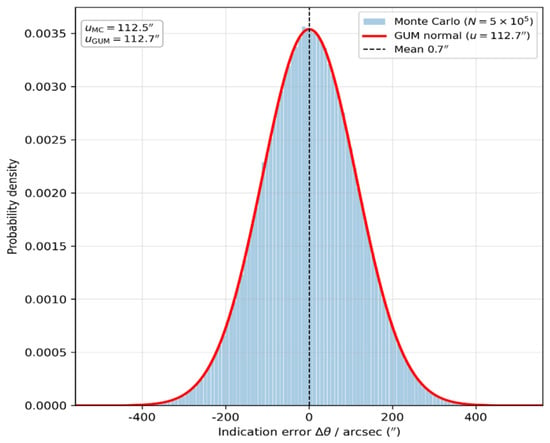
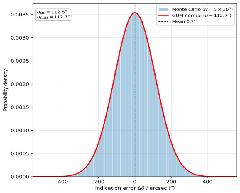
The multi-path evaluation framework proposed in this paper features universal applicability without restrictions from the single-plane decoupling zero-error working condition. Even when the test rigid body violates zero-error constraints and the ellipsoid method contains systematic bias, the eigenvector perturbation method and Monte Carlo simulation can independently quantify measurement uncertainty. The Monte Carlo histogram for indication error at the medium calibration point closely overlaps with the GUM normal fitting curve (Figure 5), validating the assumption of linear error transfer. The ellipsoid closed-form analytical expression offers intuitive formulation convenient for manual recalculation, better suited for rapid on-site engineering estimation. A clear distinction must be drawn between two independent error categories: this chapter quantifies random measurement uncertainty induced by random errors of equipment, counterweights, and positioning, where U = 0.063° characterizes the random dispersion interval of repeated calibration results. Systematic bias generated by ellipsoid simplification in Section 2.2 constitutes fixed offset monotonically increasing with inclination and asymmetry, requiring separate correction in calibration results and excluded from random uncertainty synthesis in this chapter.

Figure 5. Monte Carlo histogram and GUM normal fitting curve for indication error Δθ at medium calibration point (3.79°).

After core calculations for the medium-range calibration point 3.7869°, uncertainties for the small 2.0013° and large 6.7970° calibration points in Table 2 are calculated synchronously. Under fixed counterweight dimension conditions, full−range expanded uncertainty stabilizes within the 0.06–0.065° range with minimal fluctuation, proving excellent metrological stability of the calibration setup within the 0~7° assessment range for aerospace rotor and spacecraft principal axis inclination, capable of meeting multi-point segmented metrological calibration engineering demands.

5. Conclusions

Targeting three prominent deficiencies in existing research—inherent systematic bias of the ellipsoid method, lack of dedicated traceability schemes for principal axis inclination, and single means of uncertainty evaluation—this paper conducts integrated research covering theoretical derivation, numerical simulation, calibration methodology, and metrological evaluation, with core conclusions summarized as follows:

• Two sets of sufficient conditions yielding zero deviation between the ellipsoid method and 3D eigenvector method are derived: single-plane decoupling and transverse isotropy. A bias scaling relation is established via first-order perturbation theory: model bias varies linearly with inherent asymmetry and approximately linearly with principal axis inclination under general 3D orientations, degenerating to a cubic function of inclination only under symmetric loading special orientations. Bias equals zero strictly when δ = 0 (perfect rotational symmetry).
• A differential calibration scheme combining cylindrical standard parts and symmetric dual counterweights within the xoz plane is proposed. Symmetric counterweight layout preserves rigid-body centroid position and satisfies single-plane decoupling zero-error conditions. Three gradient calibration points (2.0013°, 3.7869°, 6.7970°) are configured to cover the common engineering range of 0–7° for segmented metrological calibration, featuring loose manufacturing constraints for standard parts and strong on-site operability.
• A multi-path joint uncertainty evaluation system integrating analytical GUM, eigenperturbation, and Monte Carlo simulation is established, with consistency among the three calculation methods superior to 0.1%. Expanded uncertainty reaches U = 0.063° (k = 2) under typical working conditions, with minimal full-range uncertainty fluctuation. I_xz, I_xx constitutes the dominant uncertainty source, and clear separation of ellipsoid model systematic bias and random measurement uncertainty is specified.
• The error theory, calibration scheme, and metrological evaluation framework developed in this paper feature strong universality, providing complete theoretical and data support for quantity traceability of aerospace rotor and spacecraft principal axis inclination measuring equipment, as well as compilation of relevant dedicated calibration specifications.
• The limitations of this study should also be noted. The bias scaling law is derived from first-order eigenperturbation theory and is quantitatively valid within the verified range of inclination 0–7° and inherent asymmetry δ ≤ 1; for larger inclinations or strongly asymmetric bodies, higher-order perturbation terms must be retained. The proposed calibration scheme is developed for cylindrical standard parts with single-plane dual-counterweight loading; its extension to standard parts of other geometries requires re-examination of the zero-error conditions and of the associated uncertainty budget. In addition, the conclusions of this paper are currently supported by theoretical derivation and numerical simulation. Future research will therefore focus on: (1) fabrication of the physical standard part and counterweight system and experimental validation of the calibration scheme on a torsional pendulum platform; (2) extension of the perturbation model to second order to cover wider inclination ranges; and (3) drafting of a dedicated calibration specification for inertial principal axis inclination based on the proposed scheme.

References

- JJF 2030—2023; Calibration Specification for Centroid Measuring Instruments Using Multi-Point Weighing Method. China Quality and Standards Publishing & Media Co., Ltd.: Beijing, China, 2023.
- JJF 2329—2025; Calibration Specification for Moment of Inertia Measuring Instruments. China Quality and Standards Publishing & Media Co., Ltd.: Beijing, China, 2025.
- JCGM 100:2008; Evaluation of Measurement Data—Guide to the Expression of Uncertainty in Measurement (GUM). BIPM: Sèvres, France, 2008.
- NIST Technical Note 1297; Guidelines for Evaluating and Expressing the Uncertainty of NIST Measurement Results. National Institute of Standards and Technology: Gaithersburg, MD, USA, 1994.
- GOST 8.207-76; Methods of Processing the Results of Observations: Basic Principles. Izdatelstvo Standartov: Moscow, Russia, 1976.
- Beer, F.P.; Johnston, E.R.; Mazurek, D.F. Vector Mechanics for Engineers: Statics, 11th ed.; McGraw-Hill: New York, NY, USA, 2016. [Google Scholar]
- Tanygin, S.; Williams, T. Mass property estimation using coasting maneuvers. J. Guid. Control Dyn. 1997, 20, 625–632. [Google Scholar] [CrossRef] [Scilit] [PubMed]
- He, X.X.; Wang, X.L.; Li, D.M. Measurement method of rotor axial unbalance based on drift trajectory. J. Tsinghua Univ. (Sci. Technol.) 2015, 55, 322–326. [Google Scholar]
- Volosov, V.V.; Kutsenko, I.A.; Selivanov, Y.A. Development and investigation of the robust ellipsoidal estimation algorithms of spacecraft inertia characteristics. J. Autom. Inf. Sci. 2005, 37, 44–57. [Google Scholar]
- Yang, K.J.; Chen, P.F. Integrated measurement system for principal inertia axis inclination and unbalance of rotors. J. Huazhong Univ. Sci. Technol. 2000, 28, 35–37. [Google Scholar]
- Zhao, J.; Guan, Y.; Qi, N.M. Analysis of determination method for principal inertia axis orientation based on dynamic balance test. China Mech. Eng. 2006, 19, 530–533. [Google Scholar] [CrossRef] [Scilit]
- Barreto, J.P.; Munoz, L.E. Low uncertainty method for inertia tensor identification. Mech. Syst. Signal Process. 2016, 68–69, 207–216. [Google Scholar] [CrossRef] [Scilit]
- Golub, G.H.; van Loan, C.F. Matrix Computations, 4th ed.; Johns Hopkins University Press: Baltimore, MD, USA, 2013. [Google Scholar]
- Chen, H. Evaluation method of measurement uncertainty for spindle rotation accuracy. Modul. Mach. Tool. Autom. Manuf. Tech. 2017, 10–17. [Google Scholar] [CrossRef]
- Wang, H. A Measuring Device and Method for Inertial Principal Axis Inclination with Multi-Source Error Compensation. Chinese Patent: CN118825647, 2026. [Google Scholar]
- Guo, F.; Lü, Z.H.; Hou, Z.C. Research on rigid body inertia parameter identification of powertrain. Automob. Technol. 2004, 8, 15–19. [Google Scholar]
- JJF 1059.1-2012; Evaluation and Expression of Measurement Uncertainty—Part 1: General. China Quality and Standards Publishing & Media Co., Ltd.: Beijing, China, 2012.
- JJF 1059.2-2012; Evaluation and Expression of Measurement Uncertainty—Part 2: Monte Carlo Method. China Quality and Standards Publishing & Media Co., Ltd.: Beijing, China, 2012.
- Schedlinski, C.; Link, M. A survey of current inertia parameter identification methods. Mech. Syst. Signal Process. 2001, 15, 189–211. [Google Scholar] [CrossRef] [Scilit]
- JJG 99-2006; Verification Regulation of Weights. China Quality and Standards Publishing & Media Co., Ltd.: Beijing, China, 2006.
- van der Ha, J.F.; Söken, H.E. Spin-axis tilt estimation algorithm with flight data. In Proceedings of the AAS/AIAA Astrodynamics Specialist Conference; AAS: Stevenson, DC, USA, 2017. [Google Scholar]
- Magnani, G.; Evain, H.; Stéphanie, D. Satellite Inertia Estimation and Observability Analysis. In Proceedings of the 9th European Conference for Aeronautics and Space Sciences (EUCASS), Lille, France, 27 June–1 July 2022. [Google Scholar]
- Zheng, S.; Dong, H.X.; Zhang, R.F. Angle estimation of a single-axis rotation: A practical inertial-measurement-unit-based method. IET Sci. Meas. Technol. 2017. [Google Scholar] [CrossRef] [Scilit]
Disclaimer/Publisher’s Note: The statements, opinions and data contained in all publications are solely those of the individual author(s) and contributor(s) and not of MDPI and/or the editor(s). MDPI and/or the editor(s) disclaim responsibility for any injury to people or property resulting from any ideas, methods, instructions or products referred to in the content. |
© 2026 by the authors. Licensee MDPI, Basel, Switzerland. This article is an open access article distributed under the terms and conditions of the Creative Commons Attribution (CC BY) license.