


Abstract
Monitoring pilot manipulation behavior is central to civil aviation safety. However, calibrated multi-camera rigs cannot be installed in a cockpit, and a single deployable depth camera yields degraded skeletons. Recognition must therefore transfer across a spatiotemporal shift dominated by a change in sensing modality. This paper proposes PRISM (Physics-Refracted Interdomain Shift Modeling). PRISM combines a cascade of degradation operators with alignment layers and treats the domain shift as separable rather than opaque. Five physics-based degradation operators are cascaded at the input, reproducing the principal error mechanisms of a depth camera. Their parameters are estimated from paired recordings rather than assumed. Two feature-space layers then align marginal distributions and class-conditional prototypes. Averaged over five seeds, combining the cascade with the two alignment layers raises the target accuracy of a spatiotemporal convolutional neural network backbone from 52.85% to 98.98% without target labels. PRISM also removes the grid search over alignment strengths. A grid search over 25 strength combinations placed its optimum at the strength combination that PRISM selects. The gain was significant on all six backbones tested, and a leave-one-subject-out rotation over the four pilots gave 98.91 ± 0.41% accuracy. The framework offers a deployable route to single-sensor cockpit monitoring.
1. Introduction
Pilot manipulation behavior is a decisive factor in civil aviation safety, and its automated monitoring has attracted sustained attention [1]. A review by the National Transportation Safety Board (NTSB) of flightcrew-involved major accidents attributed 31 of 37 cases to inadequate mutual monitoring and cross-checking performed by the crew members themselves [2]. An automatic monitor of pilot manipulation can supply an independent check when crew mutual monitoring lapses. Progress on this problem is constrained less by modeling capacity than by data. Accurate skeleton-based action recognition depends on precise three-dimensional joint coordinates. A calibrated multi-view camera rig in a laboratory environment can provide such information. However, imaging equipment intended for permanent installation in the cockpit is subject to technical airworthiness standards. Cockpit image recorder equipment, for example, must meet the China Technical Standard Order (CTSO) specification CTSO-C176a [3]. A complex laboratory multi-view rig can hardly meet such requirements. A second obstacle is vibration. During the motion of the airframe, the precise calibration results of the multi-view camera system can be easily destroyed by vibration. A single depth camera can avoid interference with pilot operation and camera calibration, and can output three-dimensional structure. However, its output is ambiguous and subject to self-occlusion, range-dependent measurement noise, and depth quantization [4].
Three lines of work bear on this problem: The first is skeleton-based action recognition, now the dominant paradigm for human motion understanding. Joint-coordinate representations discard appearance and illumination and retain only the kinematics that define an action [5]. Yan et al. [6] proposed ST-GCN, which interleaves graph convolution over an anatomical skeleton graph with temporal convolution. This has made the spatiotemporal graph the standard representation of the task. The fixed anatomical adjacency, however, cannot express relations between joints that are not physically connected. Liu et al. [7] addressed this with MS-G3D, which disentangles multi-scale graph convolutions and adds a unified spatiotemporal operator with dense cross-spacetime edges. It reached 91.5% accuracy on the NTU RGB+D 60 cross-subject split. Its multi-pathway design raises the parameter count, and its neighborhoods remain hand-specified. Chen et al. [8] proposed CTR-GCN, which learns a shared topology as a prior and refines it per channel. CTR-GCN attained 92.4% and 96.8% on the two NTU RGB+D 60 splits, and 96.5% on NW-UCLA, with few extra parameters. The refinement is driven purely by feature correlation and carries no physical interpretation.
Later work has targeted the learning objective and the representation. Chi et al. [9] proposed InfoGCN, combining an information-bottleneck objective, attention-based graph convolution, and multi-modal encoding of relative joint positions. It reached 93.0% on the NTU RGB+D 60 cross-subject split and 97.0% on NW-UCLA, but it depends on a costly ensemble of input representations. Lee et al. [10] decomposed each joint node into hierarchical sets. Their HD-GCN reached 93.4% and 97.2% on NTU RGB+D 60 under a six-way ensemble, yet the hierarchy must be predefined. Kim and Reiter [11] showed that a temporal convolutional network over joint sequences is accurate and interpretable, although skeletal structure is then only implicit. Plizzari et al. [12] replaced convolution with spatial and temporal self-attention, removing the predefined graph at quadratic cost in joints and frames. Jiang et al. [13] widened the receptive field with an inception-style multi-branch design while retaining the fixed anatomical graph. Duan et al. [14] proposed PoseConv3D, which processes skeleton sequences as 3D heatmap volumes. It is robust to pose-estimation noise and generalizes across datasets, but it discards explicit joint identity and requires two-dimensional poses. Li et al. [15] synthesized virtual viewpoints of a hand skeleton and fused them with a hierarchical aggregation network. MVHANet was competitive on three gesture benchmarks, yet its views arise from rigid transforms that reproduce no property of the sensing chain.
Two limitations are common to this body of work: First, these architectures are evaluated on benchmarks whose training and test data share one sensing chain, so sensor change is never evaluated. Second, all assume fully labeled training data. Only Tang et al. [16] framed the task as cross-dataset recognition with source-only labels, using self-supervised segmentation and permutation of temporal segments and body parts. Their method outperformed adversarial alternatives on benchmarks built from NTU RGB+D, PKU-MMD, and Kinetics. The shift that it addresses stems from viewpoint and class vocabulary rather than from a change in sensing modality.
The second line of work concerns operator-behavior monitoring in transportation, where hand and upper-body motion is used to infer distraction, secondary-task engagement, or takeover readiness. Martin et al. [17] released Drive&Act, a multi-modal in-cabin corpus of 83 hierarchically organized driver activities. Color, infrared, depth, and 3D body pose are recorded synchronously across six views, making fine-grained driver-behavior recognition a well-posed problem. However, the best reported accuracy of 69.03% on the fine-grained classes shows how difficult the setting remains, and the six-camera rig is a laboratory-grade rather than deployable installation. Qu et al. [18] surveyed vision- and learning-based driver-behavior monitoring, concluding that vision-based sensing is the most practical route to deployment. The same survey documents that existing systems are validated almost entirely on road-vehicle data and rarely report cross-setup generalization. Kim et al. [19] combined infrared facial-landmark estimation with head-pose and eye-closure modules for real-time single-device monitoring of inattention and drowsiness, reporting detection rates above 99%. The system is nevertheless confined to facial and head cues, leaving the manipulation actions by which an operator commands the vehicle outside its scope.
Comparable cockpit work is far sparser and relies predominantly on physiological or instrumented sensing rather than observation of manipulation. Li et al. [20] fused multi-modal physiological characteristics to recognize pilot behavior under increasing automation, reaching 98.15% under ten-fold cross-validation, but with body-worn instrumentation and a single-domain protocol sharing one acquisition chain. Taheri Gorji et al. [21] discriminated three cognitive-workload levels in live flight with 91.67% accuracy, using EEG features from ten pilots. This demonstrates that flight-deck state can be inferred operationally. The method, however, requires a twenty-electrode cap that cannot be carried into routine airline operation.
Two gaps follow: Vision-based monitoring is developed almost exclusively for road vehicles, whose cabin geometry and control layout differ from those of a flight deck. Also, the physiological or wearable sensing approaches adopted in current cockpit-oriented works may interfere with pilot operations.
The third line of work estimates human pose from a single depth camera—a route to single-sensor deployment, since a depth stream yields metric structure without a calibrated rig. Nguyen et al. [4] modeled the axial and lateral noise of a structured-light depth camera as functions of stand-off distance and incidence angle, improving reconstruction and tracking. However, their model describes the raw depth measurement rather than the joint coordinates that a downstream recognizer consumes. Lee et al. [22] estimated root-relative three-dimensional worker pose from a single RGB-D camera for computational dosimetry in heavily occluded radioactive environments, locating the body root through ground-plane detection and voxelized point-cloud matching. Their framework reduced mean per-joint position error by 22.7%, and by 29.2% at the wrists, without real three-dimensional pose data, yet it targets standing whole-body postures in an open workspace rather than seated fine manipulation. Hartmann et al. [23] paired marker-based motion capture with a depth sensor in a hardware-synchronized corpus of 157,825 frames. From the depth stream alone, they estimated gait parameters, obtaining up to 85.91% correct key points and a mean per-key-point error of 8.86 cm. Of that error, 2 cm to 3 cm was attributed to camera imprecision. That residual error nevertheless remains an aggregate figure, not decomposed into the underlying mechanisms that produce it. A complementary strategy exploits depth only at training time. Simoni et al. [24] trained a hallucination network to reproduce the features of a depth-pretrained backbone for monocular RGB pose estimation. Against the RGB-only baseline, it recovered 2.66 cm of mean per-joint position error. It also gained 4.5 percentage points of mean average precision at a 10 cm threshold. However, the transfer direction is opposite to that required here and is achieved by feature imitation rather than by an explicit account of sensing-chain differences.
Collectively, these studies confirm that a single depth camera is the realistically deployable configuration, yet its output is measurably noisier than multi-view triangulation. None of them decomposes the residual error into the individual physical mechanisms of the sensing chain, which an adaptation method would need in order to correct the shift rather than merely tolerate it.
These constraints explain the lack of proper data for cockpit monitoring and the importance of applying laboratory data to cockpit-monitoring model training. Stripped of its application context, this is a specific unsupervised transfer problem. A labeled source domain is available, in which holds frames of three-dimensional joint coordinates acquired by a calibrated multi-view rig, and is its action label. The target domain provides sequences of the same form . The label of is not provided during the training process. Both domains share and the joint topology, and the actions performed are nominally identical. The main difference is the sensing chain that produced the coordinates. The objective is to induce from a classifier minimizing the target risk , in which is a classification loss and is never observed. The scientific question is therefore how a structured spatiotemporal shift induced by a different sensing modality can be characterized, quantified, and removed. The problem thus stated is the province of unsupervised domain adaptation (UDA) [25,26].
Currently, three UDA paradigms dominate: The first minimizes an explicit discrepancy between source and target feature distributions. The most commonly used approaches employ the maximum mean discrepancy (MMD) or a second-order statistic. These terms are appended as regularizers to the supervised loss at one or more network layers [27,28]. The second aligns the distributions adversarially. A domain discriminator is trained to separate source from target features, while the feature extractor is trained to defeat it. Alignment is therefore enforced implicitly through a min–max game [29]. The third replaces the explicit alignment term with self-training, propagating supervision by assigning pseudo-labels to confident target samples and retraining on them [30].
A complementary line dispenses with target data altogether. Domain generalization by data augmentation perturbs source samples during training. Thus, the representation becomes invariant to the applied perturbations. The perturbations are chosen heuristically, such as additive noise, random scaling, or joint dropout [31].
These UDA approaches differ in mechanism but share one limitation: In every case, the domain shift is treated as a black box. It is measured, or implicitly countered, but never attributed to specific physical causes. There is consequently no principled basis for assigning the strength of each alignment term, and such weights are in practice set uniformly or tuned by grid search.
PRISM (Physics-Refracted Interdomain Shift Modeling) is proposed by taking that black box apart. Source and target datasets were acquired first. The source set is a multi-view laboratory dataset. The target set is a single-depth-camera cockpit dataset. Two auxiliary sets were also recorded for measurement: The first contains paired coordinates calculated from multi-view and depth captures of the same actions. The second contains raw depth frames annotated with stand-off distance and incidence angle. From the two auxiliary sets, five physics-based degradation operators, to , are parameterized. Each operator reproduces one error mechanism of the depth camera rather than applying a heuristic perturbation. The five operators are applied as a fixed cascade. The discrepancy between the two domains is re-measured after each one. This decomposes the shift under four discrepancy measures and quantifies the residual shift. The decomposition accounts for 80.10% of the initially measured MMD. That decomposition is then inverted. The contribution of each operator is normalized and mapped onto the two feature-space alignment layers. Consequently, a layer correcting a cause already compensated upstream is weakened rather than reinforced. In the process, no search over layer strengths is required.
PRISM is therefore not a replacement for feature-space alignment but a combination with it. The three layers were trained jointly under five random seeds. Target-domain accuracy rose from 52.85 ± 12.44% under direct source-only transfer to 98.98 ± 0.29%. The ablation of Section 3.3 attributes the gain to all three layers.
The main objective of this study is to enable a pilot-action recognizer trained on multi-view laboratory skeletons to be deployed on a single cockpit depth camera. No labeled target data are assumed. The route taken is to characterize, quantify, and remove the sensing-induced spatiotemporal interdomain shift explicitly. Three research questions are posed accordingly:
- RQ1: Can multi-view-to-depth transfer reach deployable recognition accuracy and calibration on cockpit data when no target label is available?
- RQ2: Can the modality-induced shift be decomposed into physically grounded degradation operators whose parameters are measured rather than assumed, and can that decomposition account for the majority of the measured discrepancy?
- RQ3: Given such a decomposition, does there exist a backbone-agnostic scheme that adaptively derives near-optimal feature-space alignment strengths from the sensing-chain information provided by the decomposition, thereby eliminating the need for explicit hyperparameter search?
The novelty of PRISM is summarized below:
- To the best of our knowledge, this research presents the first multi-view-to-depth transfer-learning dataset and model for typical civil aviation pilot actions.
- The interdomain shift is decomposed by physics-based modeling of a depth camera installed in a Boeing 737 MAX cockpit. This decomposition turns an opaque gap into an ordered set of individually quantifiable causes.
- An inverse-guided weighting strategy is proposed to set the layer strengths adaptively, requiring no hyperparameter search over unavailable target labels.
2. Materials and Methods
PRISM comprises three layers that act on a shared backbone, requiring from it only an input layer, an intermediate feature map, and an output feature vector. PRISM works like an actual prism. Its first layer L1 disperses the whole gap between multi-view triangulated and depth-camera coordinates into five physics-based degradation operators to . A prism likewise turns a beam of white light into five separable spectral lines. Each of the five operators reproduces one identifiable error mechanism of the depth camera. The reproduced mechanisms include range-dependent measurement noise, depth quantization, perspective projection with detection error, per-joint bias and jitter, and temporal jitter. Their parameters are estimated from paired recordings rather than assumed. The architecture of PRISM is shown in Figure 1.
Figure 1.
Architecture of PRISM. Layer 1 applies five physics-based degradation operators to the source set D1. The degraded source samples are fed to the backbone. Layer 2 and Layer 3 are both alignment layers, whose strengths are inverse-guided by the degradation operators.
The two remaining layers form the converging lens that refocuses the dispersed lines on the target domain. L2 aligns the marginal feature distributions through an MMD penalty at an intermediate stage of the backbone, and L3 aligns the class-conditional prototypes. Neither strength is tuned; both are assigned by an inverse-guided weighting strategy, so that what L1 has already compensated is not corrected again downstream.
2.1. Data Collection
2.1.1. Related Datasets and Rationale
Public benchmarks for skeleton-based action recognition are dominated by everyday activity recorded in laboratory settings. Nanyang Technological University (NTU) released NTU RGB+D, a red–green–blue-plus-depth action corpus that established the scale and multi-view protocol on which most subsequent methods are evaluated [32]. The Peking University Multi-Modality Dataset (PKU-MMD) extended that protocol to continuous, multi-modality sequences that must be detected as well as classified [33]. Driver-behavior corpora provide in-cabin recordings of distraction and secondary-task categories [17], while aviation-oriented datasets consist mainly of eye-tracking, flight-parameter, and simulator-log recordings rather than three-dimensional body motion [34].
To the best of our knowledge, no existing dataset can support the present study. The class vocabularies of these datasets describe whole-body activity or coarse in-cabin states, whereas pilot manipulation consists of fine actions distinguished by which control is moved and in what direction. The environments of existing datasets do not reproduce cockpit geometry, where the seat, control column, and throttle quadrant constrain both motion and line of sight. Also, none of them provides the same actions under two sensing modalities, which is exactly what a study of modality-induced shift requires. A dedicated data acquisition was therefore carried out.
2.1.2. Equipment
The choice of modality is based on practical needs. Calibrated multi-view triangulation is an accurate and complete markerless route to three-dimensional joint coordinates [35]. The rig can be installed freely in a laboratory and admits a scripted protocol, yielding a densely labeled source domain. By contrast, a single depth camera is the configuration that can realistically enter a cockpit and requires no inter-camera calibration.
Based on the chosen modalities, two sensor types were used: Depth data were acquired with a single Intel RealSense D435i depth camera (Intel Corporation, Santa Clara, CA, USA), whose depth stream was recorded at 848 × 480 pixels with a scale factor of 1.0 mm per unit. Eight Lenovo ThinkPlus WL24A USB cameras (Lenovo Group Ltd., Beijing, China) provided multi-view data for triangulation. Figure 2 shows the two sets of devices.
Figure 2.
Acquisition hardware. (a) The calibrated rig of eight RGB cameras fixed around the laboratory engineering simulator, used to record the source set; (b) the Intel RealSense D435i depth camera, used to record the target set in the cockpit environment.
During the data acquisition, two simulators were used to provide the cockpit environment. Source-domain recordings were made in a laboratory-grade engineering simulator that reproduces the forward panel, the throttle quadrant with its two thrust levers and speed brake lever, and the mode control panel (MCP). Its open frame leaves the space around the seat unobstructed, so that eight cameras can be mounted without interfering with the controls. However, this also substantially reduces its resemblance to a real cockpit. Target-domain recordings were made in a Boeing (CAE Inc., Montreal, QC, Canada) 737 MAX Level-D full-flight simulator. This is a certified device with a full-scale cockpit shell and a six-degree-of-freedom motion platform. Its seat and control column geometry is exactly the same as that of the real cockpit. The motion platform was active throughout the target-domain recordings, so both the sensor and the pilot were subject to platform motion. The resulting vibration was not instrumented, and its amplitude and spectrum are therefore not quantified in this work. In order not to obstruct the crew or the controls, both the modality and the viewpoint of the sensor were limited for the target domain. Figure 3 shows the two cockpits.
Figure 3.
Simulator environments. (a) The laboratory-grade engineering simulator for D1; (b) the Boeing 737 MAX Level-D full-flight simulator for D2.
2.1.3. Target Actions
Eight typical manipulation actions are defined here:
A1: Pulling the left and right thrust levers back at the same time, reducing the thrust of both engines simultaneously. This is commonly used at descent transition and in the landing flare.
A2: Pushing the left and right thrust levers forward at the same time, increasing the thrust of both engines simultaneously. This is commonly used at takeoff thrust set and during go-around.
A3: Controlling the left and right thrust levers separately with the left and right sides of the hand. Both levers are cross-alternated to reduce the thrust of the two engines in a staggered manner.
A4: Cross-alternating both thrust levers to increase the thrust of the two engines in a staggered manner. Both A3 and A4 are commonly used to match engine indications.
A5: Pushing the speed brake lever out to stow the speed brake. This is performed once the target speed or altitude is captured.
A6: Pulling the speed brake lever back to deploy the speed brake. This is performed when a higher descent rate or rapid deceleration is required.
A7: Turning the target-airspeed knob on the MCP, changing the selected target airspeed. This is used whenever air traffic control assigns a speed.
A8: Pressing the vertical navigation (VNAV) button on the MCP. This is used when vertical navigation is engaged after takeoff.
Three considerations govern the action selection. The eight actions span the three principal control channels of the cockpit: engine thrust (A1–A4), aerodynamic configuration (A5, A6), and autoflight (A7, A8). This action set also covers the two motion regimes that a recognizer must separate: continuous graded adjustment (A1–A7) and discrete behavior (A8). All actions are performed with the right hand by the pilot flying, in order to keep one consistent manipulation geometry. Figure 4 illustrates the eight actions.
Figure 4.
The eight pilot manipulation action classes A1 to A8. The detailed meanings of all action classes are illustrated in Section 2.1.3. All eight actions are performed by the pilot flying with the right hand.
2.1.4. Participants
Six participants took part in the data acquisition. Target-domain data were recorded by four airline pilots, P1 to P4, in the 737 MAX Level-D simulator over five sessions. All four pilots were type-rated. Source-domain data were recorded in the laboratory engineering simulator by two researchers, R1 and R2, who contributed 3997 and 819 sequences, respectively. Both R1 and R2 were briefed beforehand by the participating pilots on the details of the eight actions. Table 1 gives the participant demographics.
Table 1.
Demographics of the participants.
2.1.5. Datasets D1–D4
D1 (source domain) was recorded in the laboratory engineering simulator. Eight RGB cameras were fixed around the seat and calibrated beforehand. During collection, the subject’s right-hand actions were synchronously recorded by all cameras. AlphaPose v0.4.0 was run online on every view to localize the two-dimensional joints of the Halpe_coco_136 whole-body skeleton [36]. The detections were triangulated immediately into three-dimensional coordinates in the rig frame. Figure 5 illustrates the transition from multi-view images to spatial coordinates.
Figure 5.
Reconstruction of three-dimensional joint coordinates by multi-view triangulation. Joints are localized in each view by AlphaPose. Corresponding detections are triangulated into three-dimensional coordinates expressed in the rig frame.
D2 (target domain) was recorded in the 737 MAX Level-D simulator with a single depth camera. For D2, the color and depth streams of the single sensor were registered to a common frame by the device. AlphaPose was run on the registered color image, with the same Halpe_coco_136 model used for D1 [36]. Each detected joint pixel was then back-projected to three dimensions, using the camera intrinsics together with the registered depth value at that pixel. The resulting coordinates are expressed relative to the camera frame. Figure 6 illustrates this transition from a depth frame to spatial coordinates.
Figure 6.
Reconstruction of three-dimensional joint coordinates by a single depth camera. Two-dimensional joint detections are back-projected into three dimensions using the registered depth value and the camera intrinsics. The resulting three-dimensional coordinates are expressed in the depth-camera frame. The depth map is natively a grayscale image and is color-rendered here according to distance for visualization purposes only.
D3 (paired set) was recorded in the laboratory, adding the depth camera to the D1 rig so that the same action was captured simultaneously by both. It supplies the paired measurements from which operators to can be identified. In actual service, the mounting position of the camera and each pilot’s seat adjustment may both vary. Also, a camera installed in the cockpit cannot avoid vibration as the airframe moves. Both factors make the relative position between pilot and camera difficult to determine. Accordingly, the spatial relationship between the depth camera and the eight source-domain cameras during the D3 recordings was intentionally left unrecorded. The operators therefore describe the sensing chain only up to an unknown rigid transformation, whose residual is absorbed into and .
D4 (sensor characterization set) was recorded in the laboratory. It contains raw depth frames of body motions and of the calibration board. It was recorded at stand-off distances of roughly 0.3 m to 2.2 m, together with the camera intrinsics and depth scale. It characterizes the depth sensor itself: range-dependent noise, quantization step, and projection geometry.
2.1.6. Preprocessing
All sets passed through the same seven-stage preprocessing pipeline: (i) Units are normalized to meters. (ii) A joint is marked invalid in a frame if all three coordinates fall below 10−6 in magnitude, if any is NaN, or if its displacement from the preceding frame exceeds 0.5 m. (iii) Invalid coordinates are filled by linear interpolation between surrounding valid frames. (iv) Each series is smoothed by a Savitzky–Golay filter of window 5 and polynomial order 2 over contiguous valid segments. (v) Every frame is centered on the pelvis. (vi) Orientation is aligned based on the angle of the first-frame hip vector. (vii) Coordinates are divided by the mean neck-to-pelvis distance of the sequence, removing body-size effects.
Of the 136 Halpe_coco_136 joints, 26 were retained, including 21 right-hand joints (indices 115–135) and the left hip, right hip, head, neck, and pelvis (indices 11, 12, 17, 18, and 19). Each sequence was converted from a 3 s recording at 30 fps, so a preprocessed sample is a 26 × 90 × 3 tensor. D1 was split 90/10 into training and validation sets with random seed 42, giving 4334 training and 482 validation sequences. D2 was split by a stratified partition under the same seed into two equal halves. One half was used without labels, for distribution alignment and for the measurement of the interdomain shift only. The remaining 800 sequences form the test set for all target-domain results.
2.1.7. Dataset Statistics
D1 contains 4816 samples , in which holds frames of three-dimensional joint coordinates acquired by a calibrated multi-view rig, and is its action label. Of the 136 joints, only the 26 joints of the right hand, left hip, right hip, head, neck, and pelvis are used in this research. D2 contains 1600 similar samples , in which and . Both domains therefore share one detector and one skeleton definition, and they differ only in how the two-dimensional detections are lifted to three dimensions. Table 2 summarizes the two classification sets D1 and D2. Missing data are substantial in both sets, as expected of markerless capture of a hand repeatedly occluded. Over the 26 retained joints, 44.78% of joint–frame pairs are valid in D1, and 38.78% in D2.
Table 2.
Statistics of D1 (the source domain) and D2 (the target domain).
The 800 training sequences of D2 were used without their labels, for distribution alignment and shift measurement only.
D3 and D4 carry no class labels. D3 comprises 24 paired recordings, to , with three takes of each action. Each take stores a depth-derived and a multi-view-derived skeleton sequence with timestamps, amounting to 7839 depth and 11,282 multi-view frames. The two sensing chains were started and stopped by successive software calls on a single host, rather than by a hardware trigger. The multi-view recording window therefore brackets the depth recording window at both ends. Across the 24 takes, the depth stream started 2.56 ± 0.38 s after the multi-view stream and ended 2.52 ± 0.65 s before it. This accounted for 104.6% of the difference of 3443 frames between the two streams. The residual −4.6% is explained by the slightly lower effective frame rate of the multi-view array, at 29.34 fps against 30.11 fps. No depth frame was dropped during recording. Both streams carry per-frame host timestamps in a common clock domain. The paired sequences were aligned on that common timeline and cropped before any difference was computed.
D4 comprises 3361 depth frames aligned to the RGB stream as 16-bit unsigned integers, with intrinsics , , , and pixels. Of these, 1490 frames carry an annotated stand-off distance and incidence angle, the distances spanning 0.331 m to 2.221 m with a median of 0.733 m.
2.2. Physics-Based Decomposition of the Interdomain Shift
L1 of PRISM treats the interdomain shift as the composition of several identifiable effects. Each effect can be written as an explicit operator whose parameters are measured rather than assumed.
A source sequence is written , where indexes the retained joints and indexes the frames. Thus, represents the position of joint at frame . The binary validity mask marks the entries recovered by preprocessing. All operators leave the entries with untouched. The main idea of L1 is to map to a degraded copy through a fixed cascade:
The cascade follows the physical order of the target acquisition chain, so the operators are not interchangeable. Range-dependent noise corrupts the analog distance measurement before the sensor discretizes it (, then ). The discretized depth is combined with an image-plane joint localization that carries its own error (). The recovered three-dimensional joints inherit detector-specific systematic offsets (). The sequence is finally read out on a frame clock that is not perfectly uniform (). These five terms are selected because together they cover the dominant error mechanisms of a single active depth camera measuring a human body at close range. Ranging noise, depth quantization, projection and detection error, per-joint systematic bias and jitter, and non-uniform temporal sampling are considered. Each effect remains separable, so that the share of the shift removed by each can be quantified individually.
2.2.1. Range-Dependent Depth Noise
The stand-off distance of a joint from the depth camera is recovered as follows:
where is the depth coordinate after preprocessing and is the camera stand-off offset that restores the absolute camera-frame distance removed by root centering. The measurement noise of an active depth sensor grows with that distance, a dependence that represents as follows:
in which , , and are the quadratic, linear, and constant coefficients of the range–noise relation, respectively, is the resulting standard deviation of the depth error, is the dimensionless lateral-to-depth coupling ratio obtained from the back-projection geometry of the sensor, and is the induced in-plane error level. The operator then perturbs every valid joint and frame independently:
where , , and are the three perturbation components, and is the validity flag of that joint and frame.
2.2.2. Depth Quantization
The depth camera reports depth as an unsigned integer that is restored to meters by a fixed scale factor, so the depth coordinate is confined to a lattice; reproduces this by rounding the depth coordinate of every valid entry to the nearest multiple of the quantization step:
where is the depth quantization step in meters per least significant bit; denotes rounding to the nearest integer. The lateral coordinates are left unchanged because they are not quantized independently by the sensor.
2.2.3. Perspective Projection and Detection Noise
carries a joint through a project–perturb–back-project cycle in the image plane of the depth camera. Using focal lengths , and principal point , calibrated from D4, the joint is projected as follows:
where and are pixel coordinates. An isotropic pixel-space perturbation is applied:
with and the two perturbation components and their common standard deviation in pixels, and the result is back-projected at the unchanged depth:
The resulting lateral displacement is proportional to . As a result, the same pixel-space quantity produces a larger metric error for joints farther from the camera. This error does not exist along the line of sight. This operator therefore absorbs more than image-plane localization error alone. As mentioned before, the pose of the depth camera relative to the source-domain rig was neither constrained nor recorded. Thus, the paired measurements from which is identified also contain the residual, unmodeled extrinsic registration error between the two systems.
By construction, is zero-mean, and it leaves the depth coordinate unchanged. The systematic, joint-specific component of the lifting error, including its depth-axis part, is deferred to in Section 2.2.4.
2.2.4. Per-Joint Bias and Jitter
attaches to each joint a fixed three-dimensional offset and a frame-independent random fluctuation:
Here, is the systematic bias of joint , collects the per-axis jitter standard deviations of that joint, is the realized jitter, and forms a diagonal covariance matrix. Both and are estimated per joint. Although the two domains share the same nominal skeleton definition, the two sensing chains realize each nominal landmark at systematically different three-dimensional positions. In D1, multi-view triangulation intersects rays from eight viewpoints, so the reconstructed point lies close to the anatomical joint center inside the limb. In D2, the two-dimensional detection is lifted by sampling the registered depth map at the detected pixel. The sampled value is the depth of the camera-facing body surface. The back-projected point therefore lies on the skin rather than at the joint center. It is displaced along the line of sight by roughly half the local limb thickness, and it is further perturbed by depth-to-color registration residuals. For each joint, these effects yield a bias that is approximately constant in direction and in magnitude, together with joint- and axis-specific jitter. The operator also encodes a second fact, namely, that some landmarks are intrinsically less stable than others [37]. As with , the estimates also absorb the residual extrinsic registration error between the two sensor systems, which appears here as a component common to all joints.
is complementary to rather than a duplicate of it. captures the zero-mean, joint-homogeneous dispersion of the two-dimensional detector in the image plane. After back-projection, that dispersion acts only transversely to the viewing ray, the depth being preserved by construction. captures the non-zero-mean, joint-heterogeneous component of the lifting. This includes its dominant along-ray part, which cannot represent. Unrecorded rigid extrinsic residuals contribute to as a component shared across all joints, while their frame-level random manifestation is absorbed by .
Both parameters are estimated from D3. For each joint, the per-frame difference between the depth-derived and the multi-view-derived coordinate is collected over the paired recordings. The mean of that difference gives , and its per-axis standard deviation gives the entries of . The estimation therefore requires no annotation, only the temporal alignment described in Section 2.1.7.
2.2.5. Temporal Jitter
The depth stream and the multi-view reference are read out on independent clocks whose frame intervals are not uniform; reproduces this by resampling the sequence at perturbed frame times:
where is the nominal time index of frame for , and is its timing perturbation; is the measured standard deviation of the frame interval; ms is the nominal frame interval; is the resulting jitter expressed in frames; and keep the perturbed times monotone and inside the observed window. Each coordinate of each joint is then evaluated at those times by linear interpolation:
in which denotes piecewise-linear interpolation, with runs over the original sample times. The mask is interpolated identically and re-binarized at 0.5.
2.3. Inverse-Guided Layer-Weighting Strategy
Whereas L1 acts on the input, the two remaining layers L2 and L3 act on the representation produced by the backbone. Training minimizes the single composite objective:
is the supervised classification loss on the degraded source domain. aligns the marginal feature distributions of the two domains. aligns their class-conditional structure. are the two layer strengths whose assignment is the subject of this section.
Let be a labeled source batch to which the cascade of Equation (1) has already been applied, and an unlabeled batch from the target-training split, with . Let denote the backbone, and its feature map at layer . Let denote the average over the temporal and joint axes of a feature map. The first term of Equation (12) is the class-weighted cross-entropy:
Here, is the relative frequency of class in the source training split, so that the inverse-frequency weights sum to .
Marginal alignment (L2) is imposed on the pooled intermediate feature . This is based on a multi-scale radial-basis-function estimate of the squared MMD [27]:
where kernel and bandwidth set . is the median of all pairwise squared distances within the pooled batch. This median heuristic is re-evaluated at every step and excluded from the gradient. As a result, the three scales track the feature magnitude as it evolves, without themselves being optimized.
Class-conditional alignment (L3) operates on the pooled output feature . One prototype is maintained per class and updated from labeled source features alone by an exponential moving average with momentum [38]:
This update is detached from the gradient, and the first occurrence of a class initializes its prototype directly. Target samples carry no labels, so each is assigned to its nearest prototype, , evaluated without gradient. This assignment is the implicit pseudo-label of the current model. Writing and for the set of initialized classes with ,
This loss draws every target sample toward the source prototype of the class that it most resembles. Meanwhile, keeps the eight prototypes apart.
The two strengths are then derived from the decomposition itself rather than tuned. Let be the reduction in discrepancy metric attributable to operator , with . The metric ranges over the MMD, the correlation-alignment distance, the proxy A-distance, and the 2-Wasserstein distance. Averaging magnitudes across the metrics and rescaling to unit mean gives the raw and normalized contributions:
so that , and a value of one denotes an operator of average influence. Operators to perturb the measured coordinates themselves and, therefore, displace the feature distribution as a whole; and shift individual joints and frames in ways that alter how an action reads and, therefore, act on its class-conditional structure. The contributions are thus grouped as follows:
The strengths are then calculated with :
This inversion operation in Equation (19) is what separates this strategy from weighting each layer in proportion to the shift that it carries. What measures is the shift that L1 removes at the input, not the shift that survives into the feature space. A large identifies a mechanism that has been named, fitted to paired measurements, and explicitly reproduced on every source sample. Consequently, the corresponding part of the gap reaching the backbone is already compensated. Asking a feature-space penalty to correct it once more would act twice on the same cause. Such a correction is at best redundant and at worst destructive, distorting representations that L1 has brought into register. A small , conversely, marks a component that the physical model reproduces only weakly, whose residual is precisely what the feature-space terms must absorb. Correction strength is therefore ordered inversely to explained shift. The additive constant of 0.1 acts as a floor, preventing the layer that carries the largest weight from being switched off altogether.
2.4. Attachment to Spatiotemporal CNN Backbone
PRISM requires only three interfaces from a backbone: an input layer, an intermediate feature map, and an output feature vector consumed by the classifier. In principle, it can therefore be mounted on any architecture that exposes them. Section 3.5 examines that claim across six backbones. The spatiotemporal convolutional neural network (ST-CNN) is used here as an example, in order to explain how PRISM attaches to a backbone. Most of the experiments that follow also adopt it as the backbone, because it is simple, reliable, classical, and representative of the family.
For ST-CNN, a sample is presented as a four-channel image whose height is time and whose width is the joint index. Stacking the three coordinates with the validity flag of Equation (4) gives an input tensor of shape . Here, is the batch size, is the sequence length, and is the number of retained joints. The fourth channel tells the network which joint–frame entries are measured and which are interpolated.
Three stages follow: Stage maps its input to
Here, is a two-dimensional kernel of size convolved with stride and zero padding , is batch normalization, and is a shape-preserving residual block:
The residual block is built from two unit-stride kernels . The temporal kernel widths are and the channel widths , with and . The temporal axis is thus halved twice while the joint axis is left intact, giving stage outputs of shape , , and . A wide temporal kernel first captures the slow arm transport of an action, while later stages resolve shorter contact and release events. Global average pooling over time and joints, dropout with rate 0.2, and a single linear map then produce the class logits.
The three layers of PRISM are attached at three generic positions, and the ST-CNN is used to make each of them concrete. L1 acts at the input of the backbone, replacing the source coordinates with their degraded counterparts before the input tensor is assembled. In the ST-CNN, the three coordinate channels of the four-channel input tensor described above are therefore those produced by the cascade to . L2 acts on an intermediate feature map, taken as the deepest map that still retains spatiotemporal structure. In the ST-CNN, the marginal penalty of Equation (14) is attached at the output of stage 1, which is pooled to 128 dimensions. This is the point at which the representation is abstract enough to be compared across domains yet still carries the spatiotemporal structure that the operators to perturb. L3 acts on the output feature vector that the classifier consumes. In the ST-CNN, the class-conditional penalty of Equation (16) is attached to the 256-dimensional pooled output, where class identity is expressed. The architecture of the ST-CNN backbone with PRISM attached is shown in Figure 7.
Figure 7.
Architecture of the spatial-temporal convolutional neural network (ST-CNN) backbone. The input tensor carries the three coordinates and the validity flag of 26 joints over 90 frames. With L2 and L3 embedded, it generates the classification result. This is an example of PRISM attachment. The backbones examined in Section 3.5 attach the three layers at the corresponding positions of their own architectures.
3. Experiments and Results
Six groups of experiments were carried out: The first characterized PRISM itself, both as a reduction in the measured interdomain shift and as cross-domain classification performance on the target test split. The second comprised two comparative studies—the physics-based augmentation of L1 was set against three blind augmentation schemes; the inverse-guided weighting of Section 2.3 was set against a uniform and a proportionally guided assignment, and it was then placed on a grid search over both alignment strengths. The third was an ablation over all eight combinations of the three layers L1, L2, and L3. The fourth probed robustness by perturbing the fitted parameters of the operators to and repeating the training. The fifth substituted five further backbones for the ST-CNN. The sixth replaced the stratified target split with a leave-one-subject-out rotation over the four target-domain pilots.
All runs were executed on a laptop equipped with an NVIDIA (NVIDIA Corporation, Santa Clara, CA, USA) GeForce RTX 4090 Laptop GPU with 16 GB VRAM. The software stack was Python 3.8.20 with PyTorch 2.0.1 built against CUDA 11.8. Every network was implemented and trained in PyTorch alone.
Optimization used AdamW with an initial learning rate of 1 × 10⁻³ and weight decay 1 × 10⁻⁴. A cosine-annealing schedule with and a floor of 1 × 10⁻⁵ was applied, together with gradient-norm clipping at 1.0. The batch size was 64, and the class-weighted cross-entropy of Equation (13) was used throughout. Training ran for at most 150 epochs. It stopped early if the source validation loss had not improved for 25 consecutive epochs, the checkpoint of lowest validation loss being retained for evaluation. The splits are those defined in Section 2.1.6. D1 is divided 90/10 into training and validation sets. D2 is divided by stratified sampling into two halves. The first half serves as the unlabeled target-training set consumed by L2 and L3. The second half serves as the held-out target test set of 800 samples. Target labels were never used for training, model selection, or early stopping.
The backbone was held fixed as a controlled variable, in the same way as the optimization settings above. All results of Section 3.1, Section 3.2, Section 3.3 and Section 3.4 use the ST-CNN of Section 2.4 in the configuration described there. Section 3.5 varies the backbone alone and leaves every other setting unchanged. Section 3.6 varies the target split alone.
Every configuration reported in Section 3 was trained five times under the random seeds 42, 123, 456, 789, and 1024. The seed governs weight initialization, batch composition, and the stochastic draws inside the operators. All reported quantities are means over the five runs and are given as the mean ± standard deviation. Statistical comparisons between configurations were made with a two-sided Welch two-sample t-test on the five per-seed accuracies (n = 5 per group). No correction for multiple comparisons was applied. These five runs varied training stochasticity on one fixed data split. Variability induced by the split itself is assessed separately by the rotation of Section 3.6.
3.1. Performance of PRISM
3.1.1. Reduction in the Interdomain Shift
The shift between the source and target distributions was first measured directly on the coordinate data. All discrepancy measurements in this section were computed between the D1 training split and the unlabeled target-training half of D2 defined in Section 2.1.6. The 800-sample held-out test half of D2 was excluded. Neither the decomposition nor the layer strengths derived from it in Section 2.3 therefore draw on any data used for evaluation. Before any operator was applied, the MMD thus measured was 1.380.
The five operators were then applied in the fixed cascade order of Equation (1). Their parameters were obtained from D3 and D4, and they are reported here. For , the depth-noise model was fitted with , , and , together with an incidence-angle exponent . For , the quantization step was read from the metadata of the 16-bit depth stream rather than fitted. For , the pixel-space perturbation had . That quantity is a mixture of detection error and residual extrinsic registration error between the two systems. It is therefore not a measure of detector localization accuracy alone. For , averaged over the 21 right-hand joints, the bias magnitude was and the jitter magnitude was . The bias contains the residual rigid registration offset. Its direction and magnitude were uniform across joints, confirming that it is mainly a global translation. For , the measured timing jitter was —that is, 1.058 frames at 30 fps. The robustness study of Section 3.4 shows its effect on accuracy to be below one percentage point.
The discrepancy was re-measured after each operator. The drop attributable to an operator is the difference between the two successive measurements. The MMD waterfall in Figure 8 presents the contribution of each operator. The normalized contributions of the five operators to were 0.155, 0.003, 2.296, 1.369, and 1.176, respectively. A value of one denotes an operator of average influence. and were the two dominant mechanisms, jointly accounting for 71.9% of the initial MMD.
Figure 8.
Waterfall decomposition of the MMD shift. The leftmost bar represents the shift before any operator is applied. The rightmost bar represents the residual shift that the physics-based degradation operators do not explain. All values were computed between the D1 training split and the 800-sequence unlabeled target-training half of D2.
3.1.2. Cross-Domain Classification Performance
Classification was evaluated on the 800 held-out D2 test samples. Two configurations are reported: A source-only configuration serves as the baseline. Its ST-CNN backbone was trained on unmodified D1 with none of the three layers active and applied directly to the target domain. The second configuration is the full PRISM with L1, L2, and L3 all active as designed. Both were trained under the five seeds. They are otherwise identical in architecture, optimizer, and schedule. The split used here is the stratified split of Section 2.1.6. A subject-disjoint evaluation of the same configuration is reported in Section 3.6.
On the target test set, the source-only baseline reached an accuracy of 52.85 ± 12.44%. Its macro-averaged F1 was 47.92 ± 12.35%, and its expected calibration error (ECE) was 0.3180 ± 0.1236. Under the PRISM configuration, the same quantities were 98.98 ± 0.29%, 98.98 ± 0.28%, and 0.0082 ± 0.0026, respectively. Detailed per-class precision, recall, and F1 of the PRISM-attached ST-CNN are given in Table 3. Figure 9 shows the two confusion matrices, each averaged over the five seeds and normalized by true-class support.
Table 3.
Per-class performance of PRISM-attached ST-CNN.
Figure 9.
Confusion matrices on the target-domain test set. (a) Source-only baseline; (b) PRISM configuration. Both matrices were computed on the 800 held-out D2 test samples, averaged over the five random seeds.
3.2. Comparative Studies
3.2.1. Augmentation Strategies
The physics-based operator cascade to was compared against three augmentation schemes that perturb the source coordinates without reference to any sensing model. All configurations of this study are otherwise identical. L2 and L3 were activated with the same inverse-guided layer strengths derived for to . Only the transformation applied at L1 was varied. Let denote the coordinate of joint at frame and its validity flag from Equation (4).
The first scheme adds an isotropic Gaussian perturbation to every valid coordinate:
Here, is expressed in the normalized coordinate units left behind by stage (vii) of Section 2.1.6; is drawn independently for every joint, frame, and axis.
The second scheme drops observations independently at every joint and every frame:
A dropped observation is moved to the origin and simultaneously marked invalid. The draw is made per joint–frame pair rather than per joint, and denotes a dropped observation.
The third scheme rescales the sequence as a whole:
A single factor is drawn per training batch and shared by all samples, joints, and frames within that batch.
The baseline of this study is the configuration in which no transformation at all is applied at L1. Accuracy was recorded on the 800 held-out D2 test samples under the five random seeds. For every strategy, the relative error reduction with respect to the baseline was computed as , with . Table 4 presents the results.
Table 4.
Comparison of augmentation strategies for L1.
3.2.2. Adaptive Layer-Weighting Strategies
The three layer-weighting strategies were compared with L1, L2, and L3 all active and every other setting held fixed. The weighting strategy was therefore the only variable. Alongside the inverse-guided strategy, two arrangements were tested: The uniform baseline leaves the two alignment terms unweighted, ; therefore, it draws on no information from the decomposition. The guided strategy sets each strength equal to the corresponding layer shift weight, , which is Equation (19) with the inversion removed.
Accuracy and ECE were again recorded on the 800 held-out D2 test samples under the five random seeds. The uniform strategy served as the baseline for the significance tests. Table 5 presents the results.
Table 5.
Comparison of layer-weighting strategies.
The comparison above evaluates three specific points in the space of the two strengths. A grid search was then run in order to place those points in context. Five values of —namely, 0.10, 0.33, 0.55, 0.82, and 1.00—were crossed with five values of —namely, 0.00, 0.10, 0.50, 1.00, and 1.27. The inverse-guided assignment lies at (0.55, 0.10), the uniform baseline at (1.00, 1.00), and the guided assignment at (0.82, 1.27). Each of the 25 cells was trained under the same five random seeds, with all other settings unchanged. Figure 10 shows the resulting accuracy surface. The inverse-guided cell was the highest of the 25, at 98.98 ± 0.29%. The second highest was (0.33, 0.10), at 98.38 ± 0.35%.
Figure 10.
Accuracy surface over the grid of layer strengths. The surface gives the mean accuracy over the five random seeds on the 800 held-out D2 test samples. The translucent envelope spans the lowest and the highest of the five seeds at each grid point. The three markers give the positions of the inverse-guided, uniform, and guided assignments.
3.3. Ablation Study
The three layers of PRISM were ablated over all eight combinations of L1, L2, and L3. The eight configurations are identified below as T1 to T8. T1 is the full PRISM configuration itself with all three layers active. T2 is the configuration in which none of the three is active, which is the source-only condition. This serves as the baseline for the significance tests. All other settings remain the same for T1 to T8. Table 6 presents the results for the eight configurations.
Table 6.
Ablation of the three layers L1, L2, and L3.
A single-layer contribution was also computed for each layer as the accuracy of T1 minus the accuracy of T8, T7, and T6, respectively. Under this definition, the contributions of L1, L2, and L3 were +1.13, +0.09, and +1.75 percentage points, respectively.
3.4. Robustness Study
The sensitivity of PRISM to the values of the fitted operator parameters was examined by perturbing one operator at a time. For a given operator , every parameter was multiplied by a common factor , while the other four operators were left undisturbed. The L1-augmented source set was then regenerated, and the network was retrained under the five random seeds, with L2 and L3 active. Four perturbation levels were applied for each operator.
Accuracy on the 800 held-out D2 test samples is reported in Figure 11 as the deviation Δ from the PRISM baseline of 98.98%. Across the 20 configurations, accuracy remained between 97.48% and 99.28%. The largest decline was recorded for at , where accuracy fell by 1.50 percentage points to 97.48%. For the other 19 configurations, the deviation lay within ±1 percentage point of the baseline.
Figure 11.
Parameter sensitivity heatmap. Each perturbation was applied by multiplying every parameter of a single operator by (1 + δ). Each cell gives the deviation in accuracy from the unperturbed PRISM baseline of 98.98%, averaged over the five random seeds.
3.5. Backbone Generalization
PRISM requires only an input layer, an intermediate feature map, and an output feature vector from the backbone. Five further backbones were therefore substituted for the ST-CNN, covering the principal families of skeleton-based recognition.
The Transformer backbone [12] concatenates the three coordinates and the validity flag of all 26 joints into a single vector per frame. It projects that vector to 192 dimensions and adds a sinusoidal positional encoding. It then applies four Transformer encoder layers with eight attention heads and a feed-forward width of 896, pooling the sequence through a prepended class token.
The spatiotemporal graph convolutional network (ST-GCN) backbone [6] operates on the 26-joint skeleton graph under a distance-based spatial partition. It stacks four spatiotemporal graph-convolution blocks of 160, 160, 320, and 320 channels with a temporal kernel of five frames, followed by global pooling and a linear classifier.
The multi-view hierarchical aggregation network (MVHANet) backbone [15] rotates the skeleton into five virtual viewpoints, sampled non-uniformly so that they cluster near the frontal one. A shared co-occurrence CNN of 56 base channels encodes every view. A hierarchical attention module then aggregates views into longitude groups, and groups into one feature, weighting each by its similarity to a global context. MVHANet is designed for hand skeletons—the relevant case here, since 21 of the 26 retained joints belong to the right hand.
The MS-G3D backbone [7] stacks three blocks that sum two pathways. The unified pathway graph-convolves over the spatiotemporal graphs built from three- and five-frame sliding windows. The factorized pathway applies spatial graph convolution followed by multi-scale temporal convolution. Both pathways aggregate nine disentangled neighborhood scales, over 66, 132, and 264 channels.
The CTR-GCN backbone [8] refines the shared 26-joint topology channel by channel, inferring the refinement from pairwise joint differences within each partition subset. It stacks ten blocks of 64, 128, and 256 channels. Each block pairs that spatial unit with a four-branch temporal convolution, comprising two dilated branches, a max-pooling branch, and a 1 × 1 branch.
Every backbone was trained under the five random seeds, in the source-only configuration and in the full PRISM configuration, with only the backbone altered. The parameter counts of the six backbones all lay between 1.44 M and 2.00 M, so no architecture was given a capacity advantage. No backbone received any hyperparameter tuning under either configuration, so that performance before and after PRISM remained comparable. For each backbone, L2 was attached at the deepest intermediate feature map that the architecture exposes, following Section 2.4. The layer strengths of Section 2.3 were computed on pooled coordinates without reference to any model, so the same and apply to all six. Table 7 reports accuracy and ECE on the 800 held-out D2 test samples before and after the attachment of PRISM.
Table 7.
Backbone generalization.
Under the full configuration, the six backbones reached between 97.08% and 99.15%. The transfer gain was significant on all six, with p ≤ 0.0026. None of the five alternatives differed significantly from the ST-CNN under the full configuration, with the smallest of the five p values being 0.1138.
3.6. Subject Generalization
The stratified split of Section 2.1.6 draws the unlabeled target-training half and the test half from the same pool of recordings. Samples of one pilot therefore appear on both sides of that split. A leave-one-subject-out (LOSO) protocol was added in order to remove that overlap by construction.
The composition of D2 is first stated in full. The 1600 target samples come from four pilots over five recording sessions. Table 8 gives the recorded pilot and the sample count of every session. One pilot contributed two sessions, one of which held only 56 samples.
Table 8.
Composition of D2 by recording session.
The LOSO protocol rotates over the four pilots. In each fold, one pilot is held out. The samples of the remaining three pilots form the unlabeled target-training set consumed by L2 and L3. The samples of the held-out pilot form the test set. No target label enters training, model selection, or early stopping in any fold. The source splits of Section 2.1.6 are unchanged across folds. The four folds therefore have target-training sets of 1120, 1224, 1296, and 1160 samples, and test sets of 480, 376, 304, and 440 samples. Each fold was trained under the same five random seeds. The layer strengths were re-derived inside every fold rather than reused. Table 9 reports accuracy, macro-F1, and ECE for each fold.
Table 9.
Leave-one-subject-out results by fold.
Accuracy averaged 98.91% over the four folds. The standard deviation between the fold means was 0.41 percentage points, and the range was 0.86 percentage points, from 98.45% for P4 to 99.31% for P2. Pooling all twenty runs gave a standard deviation of 0.67 percentage points. Macro-F1 followed accuracy to two decimal places. ECE averaged 0.0118, with a between-subject standard deviation of 0.0029 and a range from 0.0094 to 0.0157. No fold effect was detected.
The input-space decomposition was also recomputed in every fold. The ordering of the five operator contributions was identical in all folds; contributed about 51% and about 20% of the initial value in every fold, and the cascade removed about 80% throughout. The physical description of the sensing chain is therefore not specific to a subset of the pilots.
4. Discussion
4.1. Performance of PRISM
PRISM effectively combines the physics-based cascade with the two alignment layers. This combination lifted the eight-class recognition accuracy on the target domain from 52.85 ± 12.44% to 98.98 ± 0.29% with the same source training set, target samples, and backbone. The main reason is that the sensing chain that produced the target coordinates is accounted for. This finding places the interdomain shift among the dominant terms of the recognition problem rather than among its nuisances. Minimizing the gap between domains without a single target label is the substantive result of this research.
For the intended application, two secondary quantities matter more than the recognition accuracy: The first is calibration. An ECE of 0.3180 means that the ST-CNN backbone without PRISM is not merely wrong but confidently wrong. Its softmax score carries almost no information about whether a prediction is correct, so there is no threshold at which an uncertain observation could be referred to a human observer. With an ECE of 0.0082, the PRISM-attached ST-CNN can defer the observations of which it is unsure instead of failing silently. In actual civil aviation operation, the worth of an automatic monitor rests on its knowing when not to be trusted. The second quantity is dispersion. Across the five seeds, the source-only baseline had a standard deviation of 12.44%, which brings unacceptable uncertainty. At 0.29% with PRISM attachment, this question no longer arises.
Figure 12 and Figure 13 show the mechanism behind those results. Both figures embed the 256-dimensional representation at the classifier input for 800 source samples of D1 and the 800 held-out target samples of D2. Markers are colored by action class, with circles denoting source and crosses denoting target. Panels (a) and (b) were produced under the source-only and the PRISM configurations, respectively.
Figure 12.
t-SNE of the joint feature space. (a) Source-only baseline; (b) PRISM configuration. Both panels embed the 256-dimensional representation at the classifier input for 800 source samples of D1 (circles) and the 800 held-out target samples of D2 (crosses). Color encodes the action classes A1 to A8.
Figure 13.
UMAP of the joint feature space. (a) Source-only baseline; (b) PRISM configuration. The samples, markers, and colors are those of Figure 12.
The improvement is clear in the t-distributed stochastic neighbor embedding (t-SNE) of Figure 12. In panel (a), the source circles occupy eight well-separated islands. This means that the baseline learns a discriminative representation, but of the source domain alone. The target crosses do not fall on those islands. For several classes, they coalesce into a single central mass in which class identity is no longer recoverable, while for a few others they stay beside the corresponding source cluster. In panel (b), every color forms one contiguous cluster holding both circles and crosses, and the eight clusters remain mutually separated. This means that the domains are aligned by class, and that the class structure survives the operation. Inside a cluster, the source and target points remain distinguishable as adjacent lobes rather than being interleaved sample by sample. This is the expected signature of alignment imposed on marginal and class-conditional distributions rather than on individual samples.
The uniform manifold approximation and projection (UMAP) embedding of Figure 13 reproduces the same reading under a different neighborhood-preserving criterion. The conclusion therefore does not rest on the choice of projection.
4.2. The Physics-Based Operators
The physics-based operator cascade to of L1 outperformed all blind augmentation schemes in the comparison experiments. Isotropic Gaussian perturbation, joint dropout, and random global scaling all displace the source data without physical reference. They enlarge the source support isotropically, or along an arbitrary and structure-free direction. Most of the mass that they add falls where no target data exist. The cascade to instead moves each source sample along the trajectory that a real measurement chain would impose on it. Every serves as a parameterized model of one measurement effect identified from the paired recordings of both sensors. As a result, its augmented samples accumulate near the target samples.
Three findings support the conclusion: First, only the effect of the to operator cascade was statistically significant across the five seeds (p = 0.0006). Second, this cascade also attained the lowest ECE of the five configurations, 0.0082, against a range of 0.0096 to 0.0144. Third, it was the only configuration that improved the mean while tightening the distribution. Its standard deviation of 0.29% is the smallest in Table 4. These results show that undirected augmentation makes the outcome depend more heavily on the seed, while directed augmentation makes it depend less on the seed. The physics-based operators adopted by PRISM therefore hold a clear advantage over blind augmentation.
4.3. The Layered Structure L1–L3
The ablation study results indicate that the three layers do not contribute the same kind of benefit. Figure 14 and Figure 15 trace the performance along the path from L3 to L2 + L3 to L1 + L2 + L3—that is, T5 to T8 to T1, alongside T2 as the baseline.
Figure 14.
Target-domain test accuracy over training. Each curve is the mean over the five random seeds, and the shaded band spans ± one standard deviation. The curves are shown to display convergence behavior only. The values reported in Table 6 are taken at the early-stopping checkpoint, so the right-hand ends of these curves are not expected to coincide with the tabulated accuracies.
Figure 15.
Target-domain test ECE over training. Each curve is the mean over the five random seeds, and the shaded band spans ± one standard deviation. As in Figure 14, the right-hand ends of these curves are not expected to coincide with the tabulated results.
L3 by itself already recovered most of the accuracy, reaching 95.83%. This indicates that class-conditional prototype alignment acts directly on the representation that the classifier consumes. Its standard deviation across seeds, however, remained 3.88%. The main cause is that prototype alignment assigns each target sample to its nearest source prototype. Since the marginal distributions can be displaced, this assignment is itself unreliable. As a result, the outcome of a run depends on the performance of early epochs. L2 addresses exactly this. L2 constrains the marginal distributions at stage 1. The dispersion fell by an order of magnitude, to 0.35 percentage points, with L2. The ECE also fell from 0.0204 to 0.0144. L1 then supplies what neither feature-space term can, removing part of the shift at the input before any representation is formed. The remaining gains in accuracy and calibration appeared there, at 98.98% and 0.0082.
The training curves make the same conclusion visible in time. In Figure 14, the T2 baseline without L1–L3 never settles. The mean accuracy wanders throughout training, and its seed band stays wide to the last epoch. The L3-only configuration does converge, but more slowly. Its band remains conspicuously wide over the first twenty epochs. The two configurations that include L2 reach their plateau within the first few epochs and hold a narrow band thereafter, with the full configuration sitting highest and flattest. Figure 15 shows the same ordering in calibration. The T2 baseline oscillates over a broad range for the whole run. The other three curves collapse within roughly twenty epochs and then stay flat, with the full configuration the lowest among them. For the application, this behavior matters as much as the final number.
The ablation study admits a second path, from T5 to T7 to T1, and it must be read alongside the first. Adding L1 to L3 alone raised accuracy from 95.83% to 98.89%. Adding L2 on top of that pair raised it only to 98.98%, an increment of 0.09 percentage points, or about one test sample in eight hundred. Taken in isolation, that path suggests that L2 is close to redundant once L1 and L3 are present. Three considerations nevertheless justify retaining it:
The first is that L2 does not depend on the other two layers in order to function. With L3 absent, adding L2 to L1 raised accuracy from 83.63% to 97.23%. With both L1 and L3 absent, L2 alone raised accuracy from 52.85% to 82.60% and reduced ECE from 0.3180 to 0.0987. The three layers act on different objects, so a failure of one does not disable the others. In an airborne application, a component that continues to provide useful behavior when its neighbors degrade is valued for that property alone.
The second consideration is that L2 is almost free. It introduces no trainable parameter. Parameter count, inference arithmetic, and peak activation memory are therefore unchanged, at 1,976,200 parameters and 1.556 G multiply–accumulate operations per sample.
The third consideration is that the increment, while small, is positive on every quantity measured. Accuracy rose by 0.09 percentage points, and ECE fell from 0.0099 to 0.0082. The configuration T7 is already close to the best result obtained in this work, so the gain available to any additional layer is small. Under that ceiling, an increment that costs nothing at inference is retained rather than discarded.
The results of the layer-weighting comparison further support the design of PRISM. The inverse-guided assignment adopted by PRISM clearly outperformed other strategies. It outperformed the baseline by 3.95 percentage points with p = 0.0044. A more informative finding is that the guided strategy reached 92.95% accuracy, falling below the uniform baseline. Under the proportional reading, the components contributing most to the shift should have received the strongest alignment, but measures the shift that L1 has already removed at the input. Pressing hardest on the features that L1 has already handled can only over-align them. The alignment term draws target features toward source features regardless of whether the resulting representation still separates the eight actions. This explains why a proportional assignment performs worse than the uniform baseline, which uses no information at all. The inverse-guided strategy allocates the remaining alignment budget to what L1 has left behind, and its advantage over both alternatives is clear and significant.
The grid search of Section 3.2.2 places that advantage on a wider map. The inverse-guided assignment was not merely better than the two alternatives. It was the best of the 25 cells examined, and the cells adjacent to it along were the next best. The inverse-guided strategy adopted by PRISM therefore recovers the optimum of the search rather than an arbitrary point inside it.
4.4. Robustness
The perturbation study yields a favorable result. The protocol is deliberately severe. Under that treatment, the target-domain accuracy never fell below 97.48%. The decline was 1.50 percentage points from the baseline in the worst of the twenty configurations and within 1 percentage point in the other nineteen. This result indicates that parameters carried over from a similar calibration, or set from a datasheet, would remain serviceable. Precise calibration of the operator parameters is therefore not a precondition for the method to work.
Sensitivity is also not uniform across the cascade. Among all operators, requires the most careful setting. This finding is consistent with the decomposition in Figure 8. accounted for the largest single share of the measured shift, a reduction of 0.710 against an initial MMD of 1.380. The operator that does most of the corrective work is also the one whose understatement is felt most. The downstream L2 and L3 can recover only some of its effect. The practical reading is that identification effort is best concentrated on , while the remaining four operators tolerate coarse settings.
4.5. Backbone Generalization Analysis
PRISM is defined in Section 2.4 as three layers acting on an input, an intermediate feature map, and an output feature vector. Section 3.5 tests whether that definition suffices in practice. Under the full configuration, the six backbones reached between 97.08% and 99.15%, and none of the five alternatives differed significantly from the ST-CNN. The transfer gain was significant on every one of the six. The benefit of PRISM is therefore not a property of one architecture, and the choice of backbone is not load-bearing for the conclusions of this work.
Two of the six backbones collapsed to chance without adaptation, and this is not a failure of representational capacity. All six fitted D1 almost exactly, with source validation accuracy of at least 98.96%, and the two collapsed models were in fact the two tightest fits. On the target set, their predictions concentrated on a single class. A model whose features had degraded to noise would produce flat logits instead. The observed behavior therefore indicates that the features were displaced as a whole, outside the region that the classifier separates.
The mechanism is a domain mismatch of the frozen batch-normalization statistics. Both collapsed backbones follow the convention of the graph-convolution literature and normalize the flattened raw coordinates at the first layer. That layer stores one source mean and variance for every joint and axis. The raw coordinates of the two domains differ by 1.42 and 1.71 source standard deviations along x and z, so the first layer already displaces its output. Both backbones also contain many normalization layers—86 and 117, respectively—whereas the ST-CNN, MVHANet, and ST-GCN have 9, 10, and 11, respectively. Each such layer rescales its input by statistics estimated on the source domain, so an offset present at the first layer is propagated and amplified. The measured offset grew from 2.8 source standard deviations at the first layer to 39 and 50 at the deepest. The Transformer contains no batch normalization, normalizing instead within each sample, and it was the strongest of the six without adaptation, at 68.55%. Its residual error of 31.45 percentage points may be read as the representational part of the gap—the part that no recalibration of statistics would remove.
PRISM removes this failure mode at its origin. Because L1 degrades the source samples into target-like form throughout training, the normalization statistics are estimated on data that already resemble the target domain. The same per-layer measurement under the full configuration gave offsets of 0.04 and 0.05 source standard deviations for the two affected backbones, against 11.95 and 21.72 without adaptation. Calibration follows: the expected calibration error fell from 0.8651 to 0.0076 and from 0.8744 to 0.0075. The layers that constitute the largest liability become an effective adaptation mechanism once their statistics are estimated on the correct distribution. This also explains why the two most fragile backbones ended among the most accurate under the full configuration.
4.6. Subject Generalization Analysis
The transductive split of Section 2.1.6 and the subject-disjoint rotation of Section 3.6 gave almost the same figure, at 98.98% and 98.91%, respectively. The difference of 0.07 percentage points is smaller than the between-subject standard deviation of 0.41 percentage points. Removing the subject overlap therefore does not reduce the reported performance.
Two observations explain why the protocol matters less here than it would in a conventional adaptation study: The first is the nature of what is being aligned. The operators to describe the sensing chain, not the person in front of it, so their parameters carry little subject-specific information. The second is the stability of the derived strengths. Re-deriving and within each fold moved them by at most 6.7% of their mean. This indicates that the measured composition of the shift is a property of the sensor pair rather than of the pilots sampled.
The LOSO experiment also evaluates the data-induced variability. The five random seeds vary weight initialization, batch composition, and the stochastic draws inside the operators, all on one fixed data split. They therefore measure training stochasticity alone. The full four-fold rotation varies the split itself, since each fold changes both the unlabeled target-training population and the test population. Across the twenty runs thus obtained, the standard deviation of accuracy was 0.67 percentage points. Variability induced by the data split is thus of the same order as variability induced by training, and neither exceeds one percentage point.
5. Conclusions
Automated monitoring of pilot manipulation behavior is held back by the difficulty of acquiring labeled three-dimensional data in a cockpit environment. The significance of this work lies in minimizing that dependence. It shows that the accuracy attainable in the laboratory with accurate joint coordinates can be carried into the cockpit of a certified Level-D full-flight simulator with a single depth camera, without labeled target samples. Also, this transfer can be made accountable. The gap between the two environments is not absorbed into an opaque adaptation mechanism but is decomposed into named physical causes. Each factor is estimated from measurement, and each carries a quantified share of the shift. The same approach applies wherever a high-fidelity modality is available for training and only a low-cost one for deployment. This is the ordinary situation of vision-based monitoring in certified or otherwise constrained environments.
The work proceeded from data collection to validation. Four datasets were recorded for the eight right-hand actions, including the source data, target data, and data supporting the alignment. Five physics-based degradation operators, to , were identified and cascaded as layer L1 to reproduce the target sensing chain. Their contributions to the interdomain shift were measured and mapped onto the two feature-space alignment layers. L2 aligns the marginal distributions; L3 aligns the class-conditional prototypes. The strengths of both layers are then assigned by the inverse-guided weighting strategy without any search over target labels. The resulting method, PRISM, was evaluated with comparison experiments, an ablation study, and a parameter-perturbation study. It was further evaluated across six backbones, and under a leave-one-subject-out rotation over the four target-domain pilots.
Table 10 places the results obtained by the PRISM-attached ST-CNN beside previously reported works. Jiang et al. [13] reported an accuracy of 96.2% on NTU RGB+D. Martin et al. [17] reported an accuracy of 69.03% on Drive&Act. Li et al. [20] reported an accuracy of 98.15% under ten-fold cross-validation. Tang et al. [16] used NTU RGB+D as the source domain and PKU-MMD as the cross-view transfer target.
Table 10.
Comparison with previously reported works.
The entries in Table 10 were drawn from different corpora and evaluated under different protocols, so the figures cannot be used for direct comparison. However, they can situate the performance of the proposed PRISM. Works [13,17,20] operate in a supervised, single-domain setting. Every training sample carries a label, and the training and test data share one sensing chain. Tang et al. [16] addressed a problem similar to that of PRISM. They transferred a skeleton recognizer across datasets and viewpoints without target labels and reached 65.5% accuracy on the target set. PRISM reached 98.98 ± 0.29% on eight pilot manipulation classes under a similar regime. While the figures are not directly comparable, the result places PRISM at the upper end of the range reported previously.
With respect to the main objective and the three research questions formulated in Section 1, the experiments conducted here support the following answers:
RQ1 is answered in the affirmative. Multi-view-to-depth transfer is feasible for the civil aviation cockpit. Without a single target label, target-domain accuracy rose from 52.85 ± 12.44% to 98.98 ± 0.29%, and ECE fell from 0.3180 to 0.0082. The seed-to-seed dispersion contracted to 0.29 percentage points. A leave-one-subject-out rotation over the four pilots gave 98.91 ± 0.41%, with no fold effect detected. The transfer gain was significant on all six backbones examined. The main objective is therefore achieved within the scope of the eight actions considered.
RQ2 is answered in the affirmative. The five physics-based operators accounted for 80.10% of the initially measured MMD, and every operator parameter was estimated from measurement rather than assumed. The improvement brought by the to cascade was statistically significant across the five seeds (p = 0.0006). The cascade also degrades gracefully when its parameters are coarse. The shift can therefore be treated as separable rather than opaque, with a residual 19.90% left to the two feature-space layers.
RQ3 is answered in the affirmative. The proposed inverse-guided strategy adopted by PRISM was significantly better than assigning the two alignment strengths uniformly (p = 0.0044). The proportional variant built from the same decomposition fell below the uniform baseline. A grid search over 25 combinations of the two strengths placed its own optimum at the cell that the rule selects, so no search over target labels is required. The decomposition measures the shift that L1 has already removed at the input, and alignment strength must therefore be ordered inversely to the shift explained.
These affirmative answers hold within the scope defined by the data and the physical model. Four limitations bound them:
The first is the data limitation. Joints outside the right hand are severely under-populated in the present datasets, so the transfer study is confined to right-hand manipulation actions. The recordings also cover the pilot flying only. Usually, the pilot monitoring performs the same eight actions with the left hand, and the resulting manipulation geometry is mirrored. Whether a recognizer trained on one seat transfers to the other is therefore untested. Extending the work to both seats, to whole-body posture, and to the interaction between the two crew members requires better data coverage.
The second is the physical model. Five operators were modeled, but other factors were ignored. Factors such as illumination change over a flight and mutual occlusion between crew members are outside the present formulation.
The third is the task formulation. Recognition is posed as a closed-set problem over eight classes, with no class for the absence of a defined action. Continuous monitoring in service would require open-set rejection of actions outside the vocabulary. This is not addressed here.
The fourth is the subject scale. The source data were recorded by two researchers and the target data by four airline pilots. A leave-one-subject-out rotation over the four pilots gave 98.91 ± 0.41%, and no fold effect was detected. Four folds nevertheless afford little statistical power, and a cohort of four cannot represent the variation in a pilot population. A larger cohort is needed before the reported figures can be read as subject-independent.
Author Contributions
Conceptualization, Y.S.; methodology, Y.S.; software, Y.S.; validation, G.X.; formal analysis, Y.S.; investigation, Y.S.; resources, G.X.; data curation, Y.S. and L.L.; writing—original draft preparation, Y.S.; writing—review and editing, G.X. and G.W.; visualization, L.Z.; supervision, G.X.; project administration, G.X. All authors have read and agreed to the published version of the manuscript.
Funding
This research received no external funding.
Informed Consent Statement
Verbal informed consent was obtained from all subjects involved in the study prior to data acquisition. All six participants were informed of the purpose of the study, the recording modalities used, the nature of the data to be collected, and their right to withdraw at any time without consequence. Verbal informed consent has also been obtained from the participants to publish the images and the derived joint-coordinate data presented in this paper, and to release the datasets D1–D4 in a public repository. All released data consist of three-dimensional joint coordinates from which no facial or other directly identifying information can be recovered.
Data Availability Statement
The datasets D1–D4 generated and analyzed in this study are openly available in Mendeley Data at https://doi.org/10.17632/jpnwbtyjz7.1, reference number [39].
Acknowledgments
The authors thank the four type-rated airline pilots who recorded the target-domain data in the Boeing 737 MAX Level-D simulator, as well as the two researchers who recorded the source-domain data in the laboratory engineering simulator, for their time and cooperation during data acquisition.
Conflicts of Interest
The authors declare that they have no known competing financial interests or personal relationships that could have appeared to influence the work reported in this paper.
Abbreviations
The following abbreviations are used in this manuscript:
| CTR-GCN | Channel-wise topology refinement graph convolutional network |
| CTSO | China Technical Standard Order |
| CUDA | Compute Unified Device Architecture |
| ECE | Expected calibration error |
| GPU | Graphics processing unit |
| LOSO | Leave-one-subject-out |
| MCP | Mode control panel |
| MMD | Maximum mean discrepancy |
| MS-G3D | Multi-scale disentangled unified graph convolutional network |
| MVHANet | Multi-view hierarchical aggregation network |
| NaN | Not a number |
| NTSB | National Transportation Safety Board |
| NTU | Nanyang Technological University |
| PKU-MMD | Peking University Multi-Modality Dataset |
| PRISM | Physics-Refracted Interdomain Shift Modeling |
| RGB | Red, green, and blue |
| RQ | Research question |
| ST-CNN | Spatiotemporal convolutional neural network |
| ST-GCN | Spatiotemporal graph convolutional network |
| t-SNE | t-Distributed stochastic neighbor embedding |
| UDA | Unsupervised domain adaptation |
| UMAP | Uniform manifold approximation and projection |
| USB | Universal serial bus |
| VNAV | Vertical navigation |
| VRAM | Video random-access memory |
References
- Jarvis, S.R. Concurrent Pilot Instrument Monitoring in the Automated Multi-Crew Airline Cockpit. Aerosp. Med. Hum. Perform. 2017, 88, 1100–1106. [Google Scholar] [CrossRef] [Scilit] [PubMed]
- National Transportation Safety Board. A Review of Flightcrew-Involved Major Accidents of U.S. Air Carriers, 1978 through 1990. In Safety Study NTSB/SS-94/01; National Transportation Safety Board: Washington, DC, USA, 1994. [Google Scholar]
- Civil Aviation Administration of China. Cockpit Image Recorder Equipment; China Civil Aviation Technical Standard Order CTSO-C176a; Civil Aviation Administration of China: Beijing, China, 2018. Available online: https://www.caac.gov.cn/XXGK/XXGK/BZGF/JSBZGD/201901/t20190103_193814.html (accessed on 5 September 2026).
- Nguyen, C.V.; Izadi, S.; Lovell, D. Modeling Kinect Sensor Noise for Improved 3D Reconstruction and Tracking. In Proceedings of the Second International Conference on 3D Imaging, Modeling, Processing, Visualization and Transmission, Zurich, Switzerland, 13–15 October 2012; pp. 524–530. [Google Scholar] [CrossRef] [Scilit]
- Xin, W.; Liu, R.; Liu, Y.; Chen, Y.; Yu, W.; Miao, Q. Transformer for Skeleton-Based Action Recognition: A Review of Recent Advances. Neurocomputing 2023, 537, 164–186. [Google Scholar] [CrossRef] [Scilit]
- Yan, S.; Xiong, Y.; Lin, D. Spatial Temporal Graph Convolutional Networks for Skeleton-Based Action Recognition. In Proceedings of the Thirty-Second AAAI Conference on Artificial Intelligence, New Orleans, LA, USA, 2–7 February 2018. [Google Scholar] [CrossRef] [Scilit]
- Liu, Z.; Zhang, H.; Chen, Z.; Wang, Z.; Ouyang, W. Disentangling and Unifying Graph Convolutions for Skeleton-Based Action Recognition. In Proceedings of the IEEE/CVF Conference on Computer Vision and Pattern Recognition, Seattle, WA, USA, 13–19 June 2020; pp. 143–152. [Google Scholar] [CrossRef] [Scilit]
- Chen, Y.; Zhang, Z.; Yuan, C.; Li, B.; Deng, Y.; Hu, W. Channel-Wise Topology Refinement Graph Convolution for Skeleton-Based Action Recognition. In Proceedings of the IEEE/CVF International Conference on Computer Vision, Montreal, QC, Canada, 10–17 October 2021; pp. 13339–13348. [Google Scholar] [CrossRef] [Scilit]
- Chi, H.-g.; Ha, M.H.; Chi, S.; Lee, S.W.; Huang, Q.; Ramani, K. InfoGCN: Representation Learning for Human Skeleton-Based Action Recognition. In Proceedings of the IEEE/CVF Conference on Computer Vision and Pattern Recognition, New Orleans, LA, USA, 18–24 June 2022; pp. 20154–20164. [Google Scholar] [CrossRef] [Scilit]
- Lee, J.; Lee, M.; Lee, D.; Lee, S. Hierarchically Decomposed Graph Convolutional Networks for Skeleton-Based Action Recognition. In Proceedings of the IEEE/CVF International Conference on Computer Vision, Paris, France, 1–6 October 2023; pp. 10410–10419. [Google Scholar] [CrossRef] [Scilit]
- Kim, T.S.; Reiter, A. Interpretable 3D Human Action Analysis with Temporal Convolutional Networks. In Proceedings of the IEEE Conference on Computer Vision and Pattern Recognition Workshops, Honolulu, HI, USA, 21–26 July 2017; pp. 1623–1631. [Google Scholar] [CrossRef] [Scilit]
- Plizzari, C.; Cannici, M.; Matteucci, M. Skeleton-Based Action Recognition via Spatial and Temporal Transformer Networks. Comput. Vis. Image Underst. 2021, 208–209, 103219. [Google Scholar] [CrossRef] [Scilit]
- Jiang, M.; Dong, J.; Ma, D.; Sun, J.; He, J.; Lang, L. Inception Spatial Temporal Graph Convolutional Networks for Skeleton-Based Action Recognition. In Proceedings of the 2022 International Symposium on Control Engineering and Robotics, Changsha, China, 26–27 February 2022; pp. 208–213. [Google Scholar] [CrossRef] [Scilit]
- Duan, H.; Zhao, Y.; Chen, K.; Lin, D.; Dai, B. Revisiting Skeleton-Based Action Recognition. In Proceedings of the IEEE/CVF Conference on Computer Vision and Pattern Recognition, New Orleans, LA, USA, 18–24 June 2022; pp. 2969–2978. [Google Scholar] [CrossRef] [Scilit]
- Li, S.; Liu, Z.; Duan, G.; Tan, J. MVHANet: Multi-View Hierarchical Aggregation Network for Skeleton-Based Hand Gesture Recognition. Signal Image Video Process. 2023, 17, 2521–2529. [Google Scholar] [CrossRef] [Scilit]
- Tang, Y.; Liu, X.; Yu, X.; Zhang, D.; Lu, J.; Zhou, J. Learning from Temporal Spatial Cubism for Cross-Dataset Skeleton-Based Action Recognition. ACM Trans. Multimed. Comput. Commun. Appl. 2022, 18, 46. [Google Scholar] [CrossRef] [Scilit] [PubMed]
- Martin, M.; Roitberg, A.; Haurilet, M.; Horne, M.; Reiß, S.; Voit, M.; Stiefelhagen, R. Drive&Act: A Multi-Modal Dataset for Fine-Grained Driver Behavior Recognition in Autonomous Vehicles. In Proceedings of the IEEE/CVF International Conference on Computer Vision, Seoul, Republic of Korea, 27 October–2 November 2019; pp. 2801–2810. [Google Scholar] [CrossRef] [Scilit]
- Qu, F.; Dang, N.; Furht, B.; Nojoumian, M. Comprehensive Study of Driver Behavior Monitoring Systems Using Computer Vision and Machine Learning Techniques. J. Big Data 2024, 11, 32. [Google Scholar] [CrossRef] [Scilit]
- Kim, D.; Park, H.; Kim, T.; Kim, W.; Paik, J. Real-Time Driver Monitoring System with Facial Landmark-Based Eye Closure Detection and Head Pose Recognition. Sci. Rep. 2023, 13, 18264. [Google Scholar] [CrossRef] [Scilit] [PubMed]
- Li, Y.; Li, K.; Wang, S.; Chen, X.; Wen, D. Pilot Behavior Recognition Based on Multi-Modality Fusion Technology Using Physiological Characteristics. Biosensors 2022, 12, 404. [Google Scholar] [CrossRef] [Scilit] [PubMed]
- Taheri Gorji, H.; Wilson, N.; VanBree, J.; Hoffmann, B.; Petros, T.; Tavakolian, K. Using Machine Learning Methods and EEG to Discriminate Aircraft Pilot Cognitive Workload during Flight. Sci. Rep. 2023, 13, 2507. [Google Scholar] [CrossRef] [Scilit] [PubMed]
- Lee, J.; Cho, W.; Jang, S.; Lee, M.; Shin, S.-G.; Han, S.; Jo, H.; Kim, S. 3D Pose Estimation of Workers in Complex Radioactive Environments Using a Single RGB-D Camera. Nucl. Eng. Technol. 2025, 57, 103631. [Google Scholar] [CrossRef] [Scilit]
- Hartmann, Y.; Paul, R.E.; Klöckner, J.; Deichsel, L.; Schultz, T. Gait Parameter Estimation from a Single Depth Sensor. J. Smart Cities Soc. 2025, 4, 35–61. [Google Scholar] [CrossRef] [Scilit]
- Simoni, A.; Marchetti, F.; Borghi, G.; Becattini, F.; Davoli, D.; Garattoni, L.; Francesca, G.; Seidenari, L.; Vezzani, R. Depth-Based Privileged Information for Boosting 3D Human Pose Estimation on RGB. In Computer Vision—ECCV 2024 Workshops; Lecture Notes in Computer Science; Springer: Cham, Switzerland, 2025; Volume 15635, pp. 189–203. [Google Scholar] [CrossRef] [Scilit]
- Ben-David, S.; Blitzer, J.; Crammer, K.; Kulesza, A.; Pereira, F.; Vaughan, J.W. A Theory of Learning from Different Domains. Mach. Learn. 2010, 79, 151–175. [Google Scholar] [CrossRef] [Scilit]
- Wilson, G.; Cook, D.J. A Survey of Unsupervised Deep Domain Adaptation. ACM Trans. Intell. Syst. Technol. 2020, 11, 51. [Google Scholar] [CrossRef] [Scilit] [PubMed]
- Yu, S.; Song, L.; Pang, S.; Wang, M.; He, X.; Xie, P. M-Net: A Novel Unsupervised Domain Adaptation Framework Based on Multi-Kernel Maximum Mean Discrepancy for Fault Diagnosis of Rotating Machinery. Complex Intell. Syst. 2024, 10, 3259–3272. [Google Scholar] [CrossRef] [Scilit]
- Sun, B.; Saenko, K. Deep CORAL: Correlation Alignment for Deep Domain Adaptation. In Computer Vision—ECCV 2016 Workshops; Hua, G., Jégou, H., Eds.; Lecture Notes in Computer Science; Springer: Cham, Switzerland, 2016; Volume 9915, pp. 443–450. [Google Scholar] [CrossRef] [Scilit]
- Gallego, A.-J.; Calvo-Zaragoza, J.; Fisher, R.B. Incremental Unsupervised Domain-Adversarial Training of Neural Networks. IEEE Trans. Neural Netw. Learn. Syst. 2021, 32, 4864–4878. [Google Scholar] [CrossRef] [Scilit] [PubMed]
- Zou, Y.; Yu, Z.; Vijaya Kumar, B.V.K.; Wang, J. Unsupervised Domain Adaptation for Semantic Segmentation via Class-Balanced Self-Training. In Computer Vision—ECCV 2018; Ferrari, V., Hebert, M., Sminchisescu, C., Weiss, Y., Eds.; Lecture Notes in Computer Science; Springer: Cham, Switzerland, 2018; Volume 11207, pp. 297–313. [Google Scholar] [CrossRef] [Scilit]
- Volpi, R.; Namkoong, H.; Sener, O.; Duchi, J.C.; Murino, V.; Savarese, S. Generalizing to Unseen Domains via Adversarial Data Augmentation. In Proceedings of the 32nd International Conference on Neural Information Processing Systems, Montréal, QC, Canada, 3–8 December 2018. [Google Scholar]
- Shahroudy, A.; Liu, J.; Ng, T.-T.; Wang, G. NTU RGB+D: A Large Scale Dataset for 3D Human Activity Analysis. In Proceedings of the IEEE Conference on Computer Vision and Pattern Recognition, Las Vegas, NV, USA, 27–30 June 2016; pp. 1010–1019. [Google Scholar] [CrossRef] [Scilit]
- Liu, C.; Hu, Y.; Li, Y.; Song, S.; Liu, J. PKU-MMD: A Large Scale Benchmark for Continuous Multi-Modal Human Action Understanding. arXiv 2017, arXiv:1703.07475. [Google Scholar] [CrossRef] [Scilit]
- Fettrow, T.; Stephens, C.; Prinzel, L.; Holbrook, J.; Ballard, K.; Bastami, S.; Stewart, M.; Kiggins, D. Human Contributions to Safety Data Testbed Flight Simulation Study: Data Methods, Processing, and Quality. Sci. Data 2025, 12, 1247. [Google Scholar] [CrossRef] [Scilit] [PubMed]
- Nakano, N.; Sakura, T.; Ueda, K.; Omura, L.; Kimura, A.; Iino, Y.; Fukashiro, S.; Yoshioka, S. Evaluation of 3D Markerless Motion Capture Accuracy Using OpenPose with Multiple Video Cameras. Front. Sports Act. Living 2020, 2, 50. [Google Scholar] [CrossRef] [Scilit] [PubMed]
- Fang, H.-S.; Li, J.; Tang, H.; Xu, C.; Zhu, H.; Xiu, Y.; Li, Y.-L.; Lu, C. AlphaPose: Whole-Body Regional Multi-Person Pose Estimation and Tracking in Real-Time. IEEE Trans. Pattern Anal. Mach. Intell. 2023, 45, 7157–7173. [Google Scholar] [CrossRef] [Scilit] [PubMed]
- Needham, L.; Evans, M.; Cosker, D.P.; Wade, L.; McGuigan, P.M.; Bilzon, J.L.; Colyer, S.L. The Accuracy of Several Pose Estimation Methods for 3D Joint Centre Localisation. Sci. Rep. 2021, 11, 20673. [Google Scholar] [CrossRef] [Scilit] [PubMed]
- Sidibomma, R.; Sanodiya, R.K. Learning Semantic Representations and Discriminative Features in Unsupervised Domain Adaptation. In Proceedings of the 11th International Symposium on Electronic Systems Devices and Computing, Sri City, India, 4–6 May 2023; pp. 1–6. [Google Scholar] [CrossRef] [Scilit]
- Shen, Y. Civil Cockpit Multi-View-to-Depth Transfer. Mendeley Data, V1, 2026. Available online: https://data.mendeley.com/datasets/jpnwbtyjz7/1 (accessed on 8 September 2026).
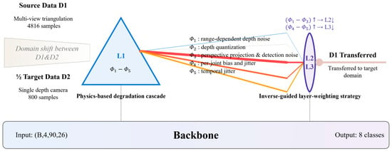
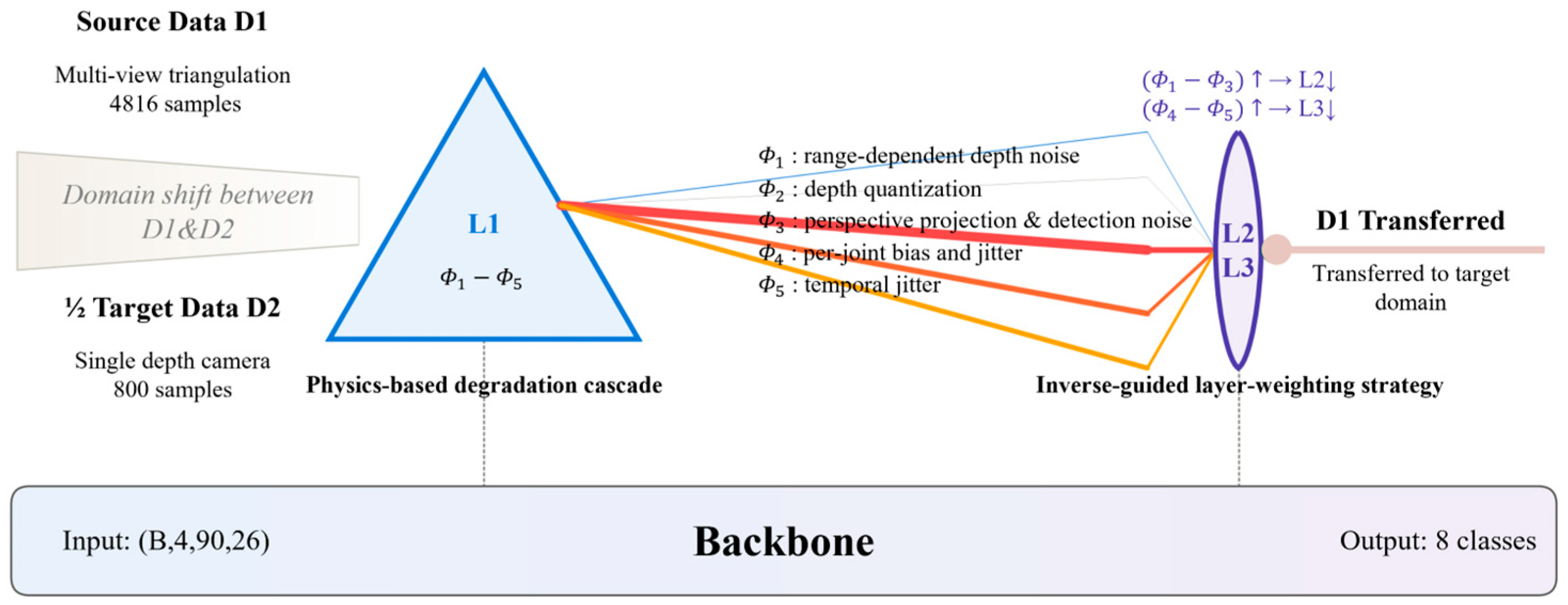
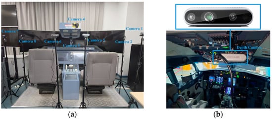
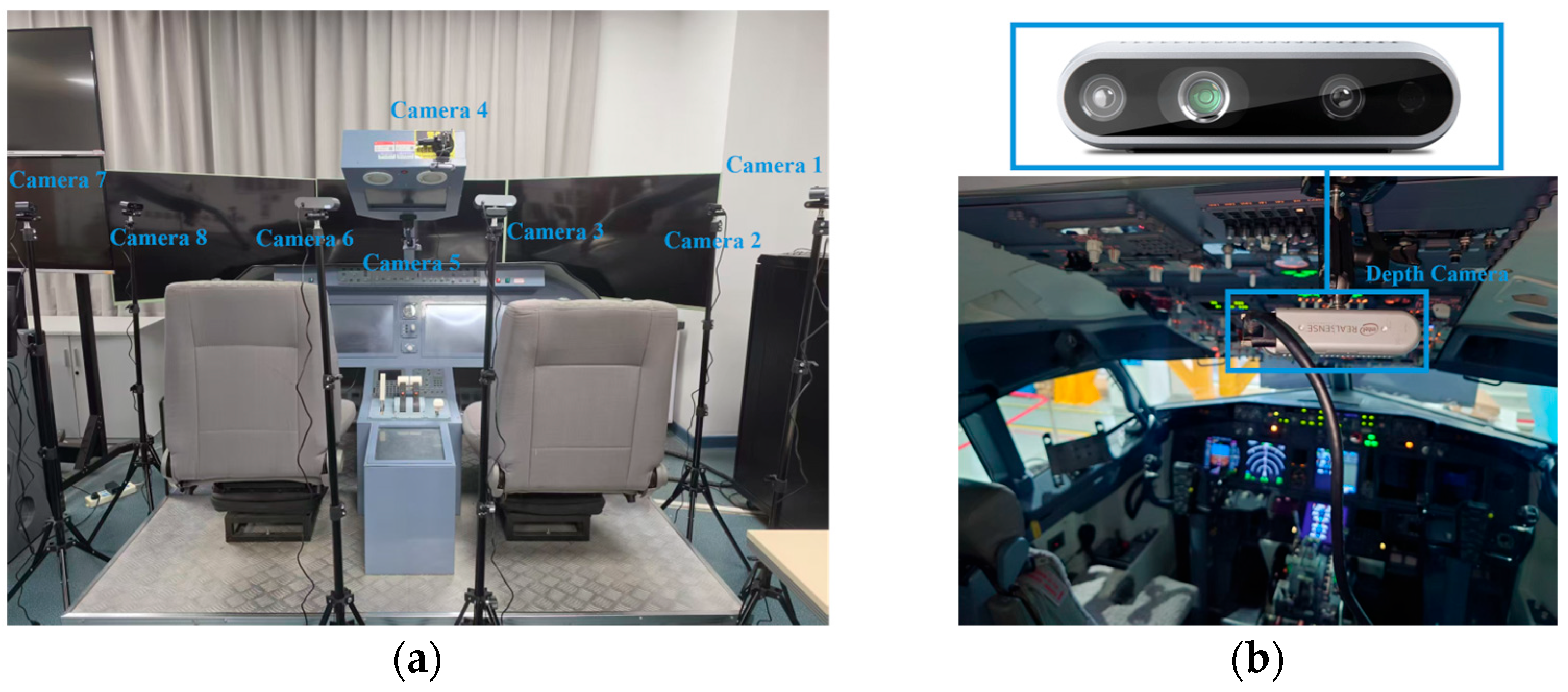
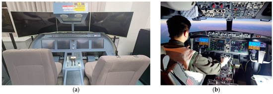
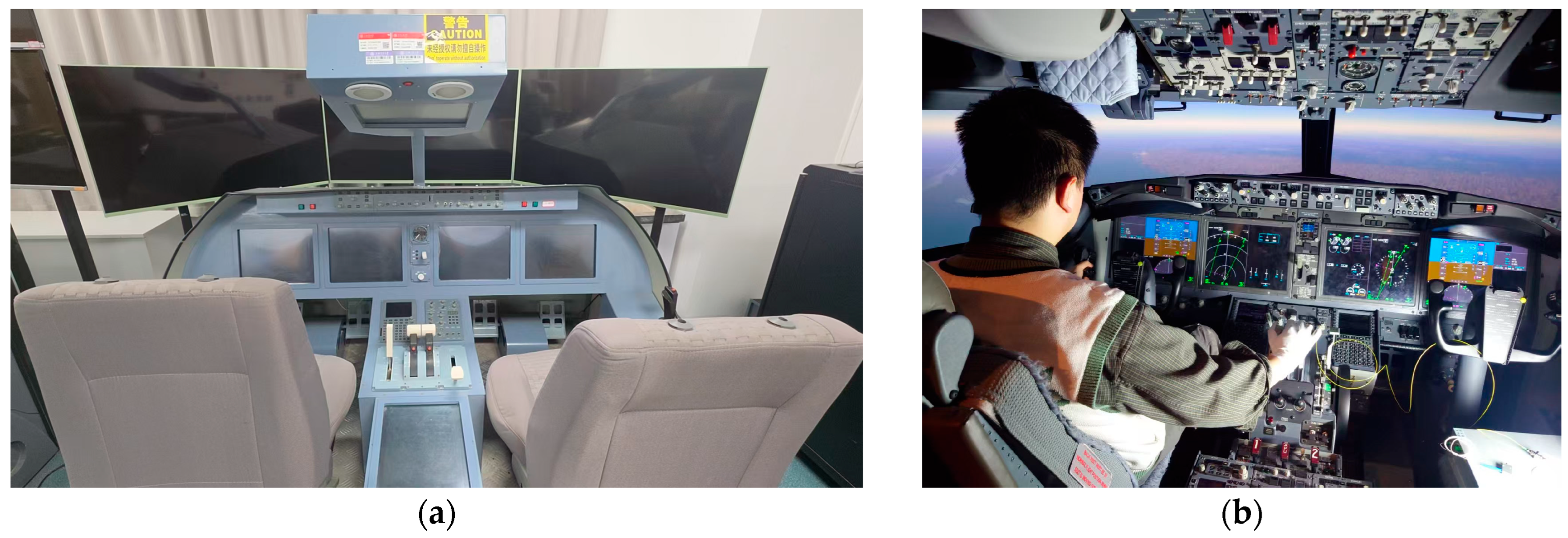
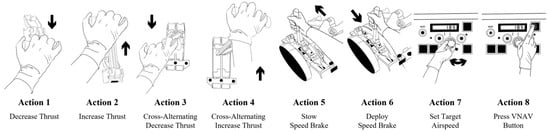
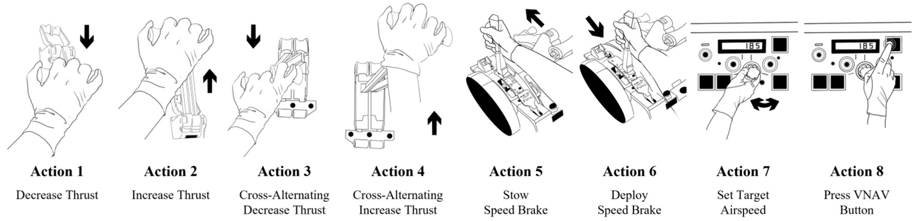
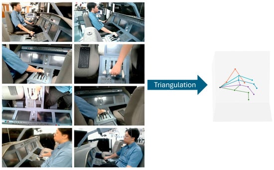
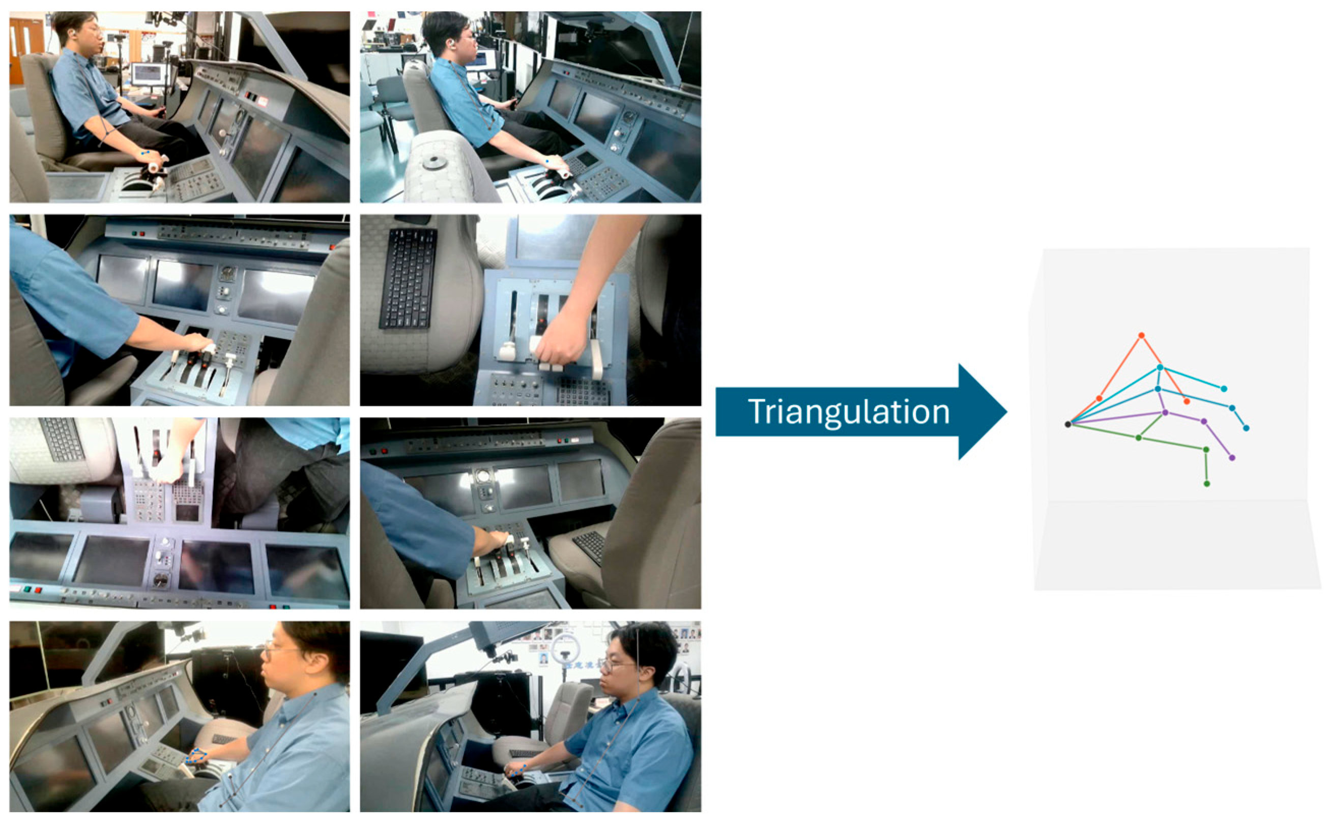
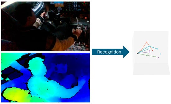
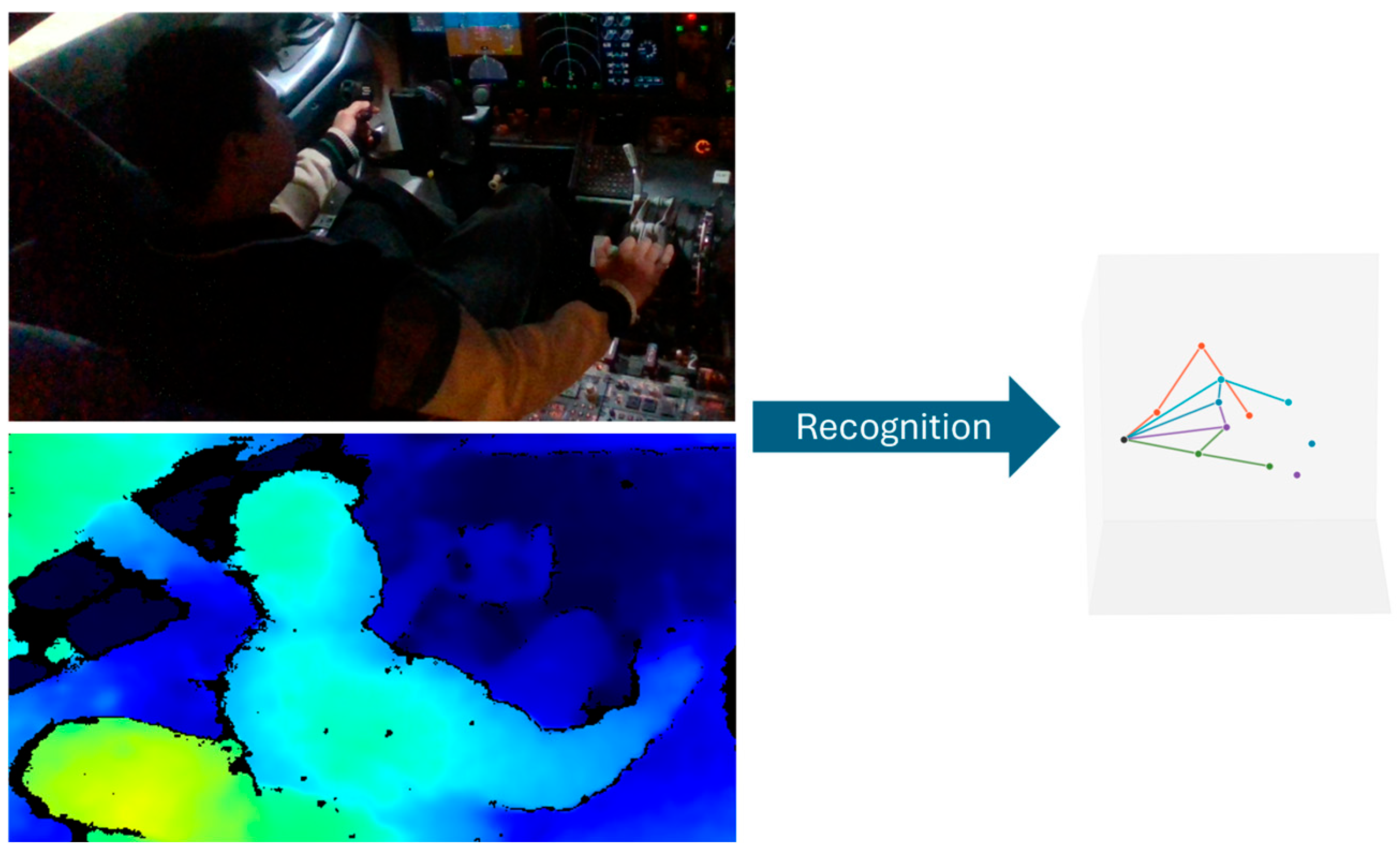
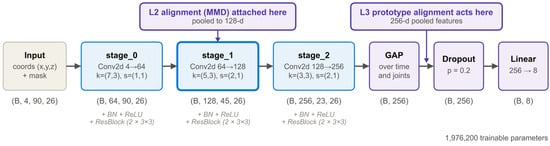
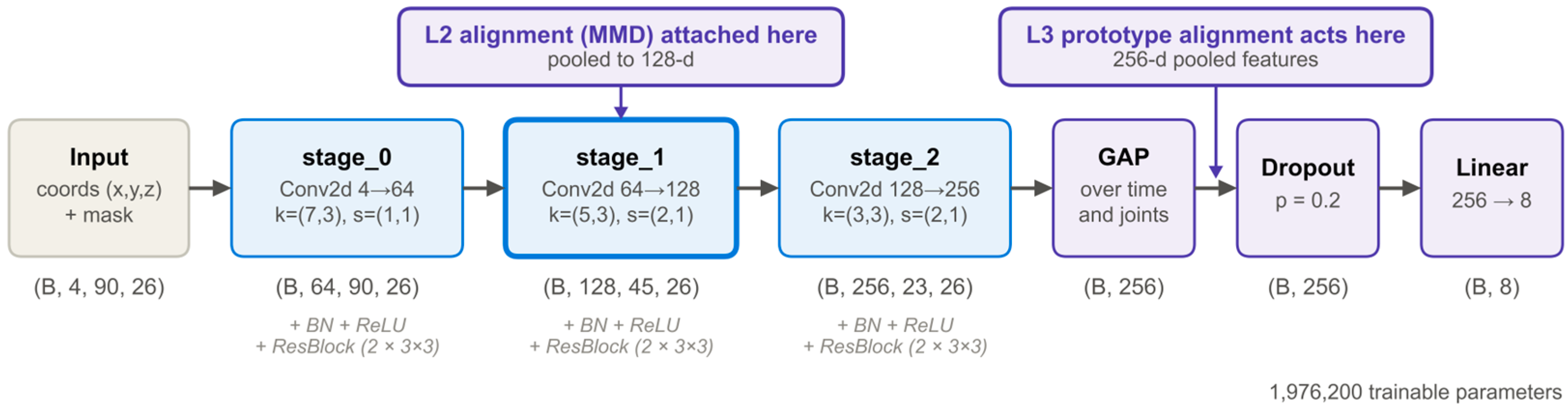
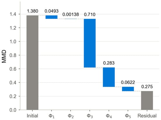
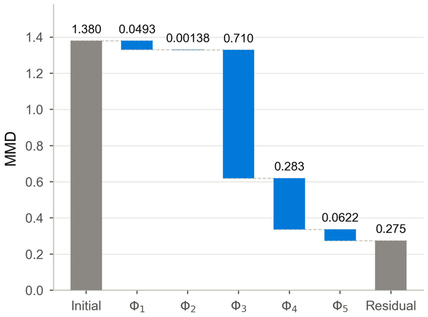
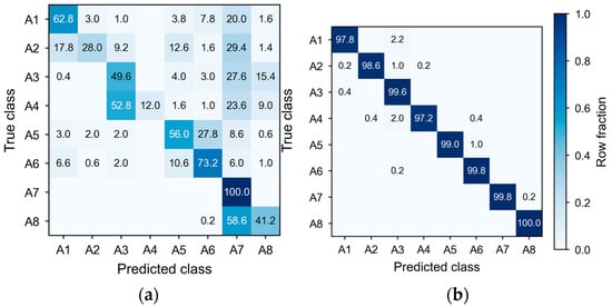
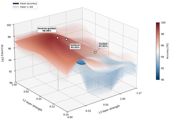
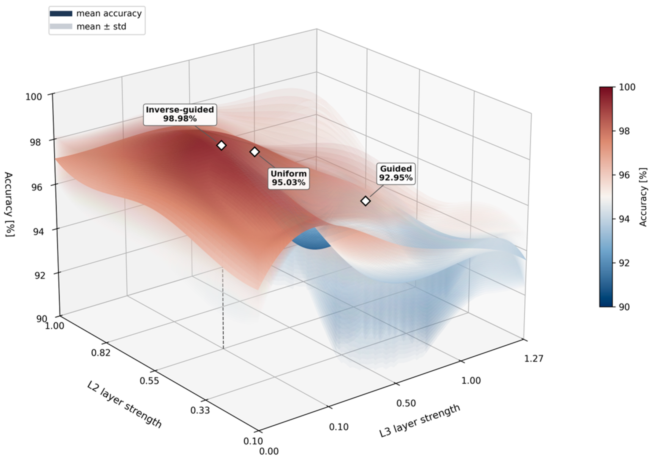
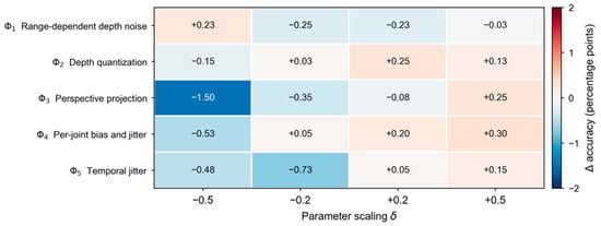
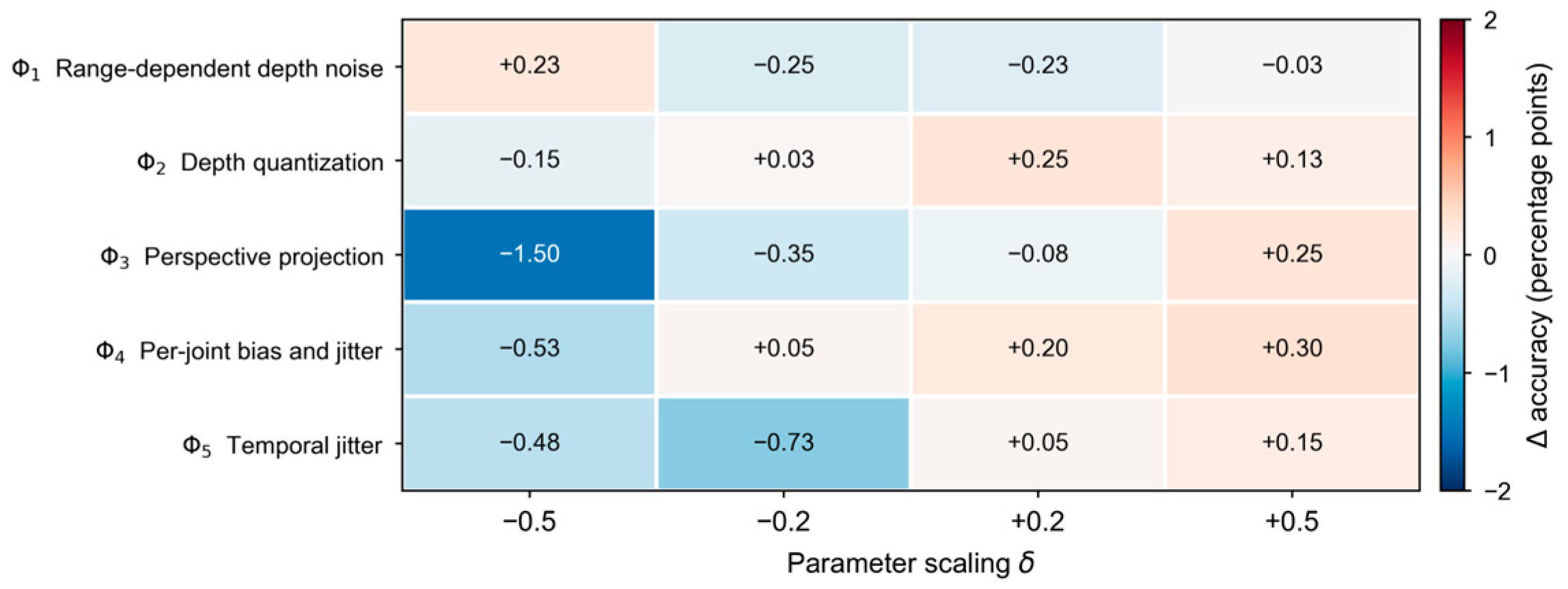
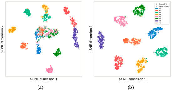
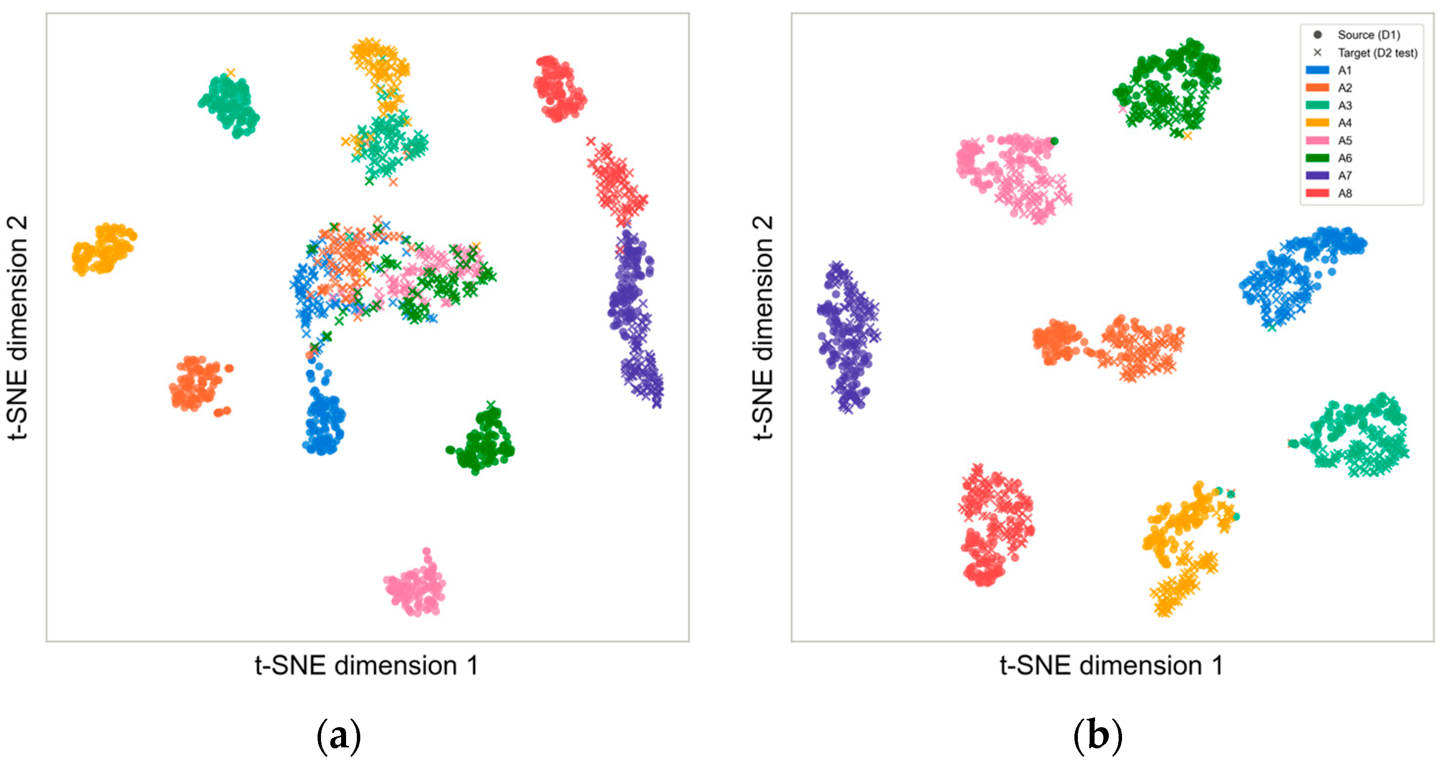
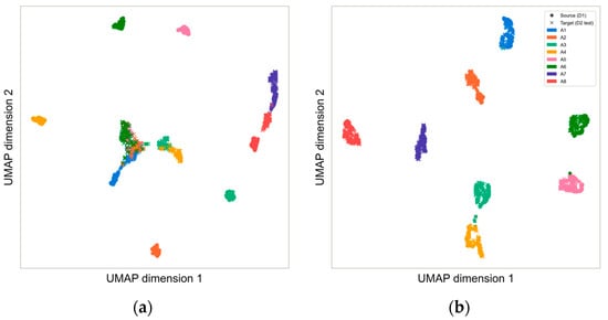
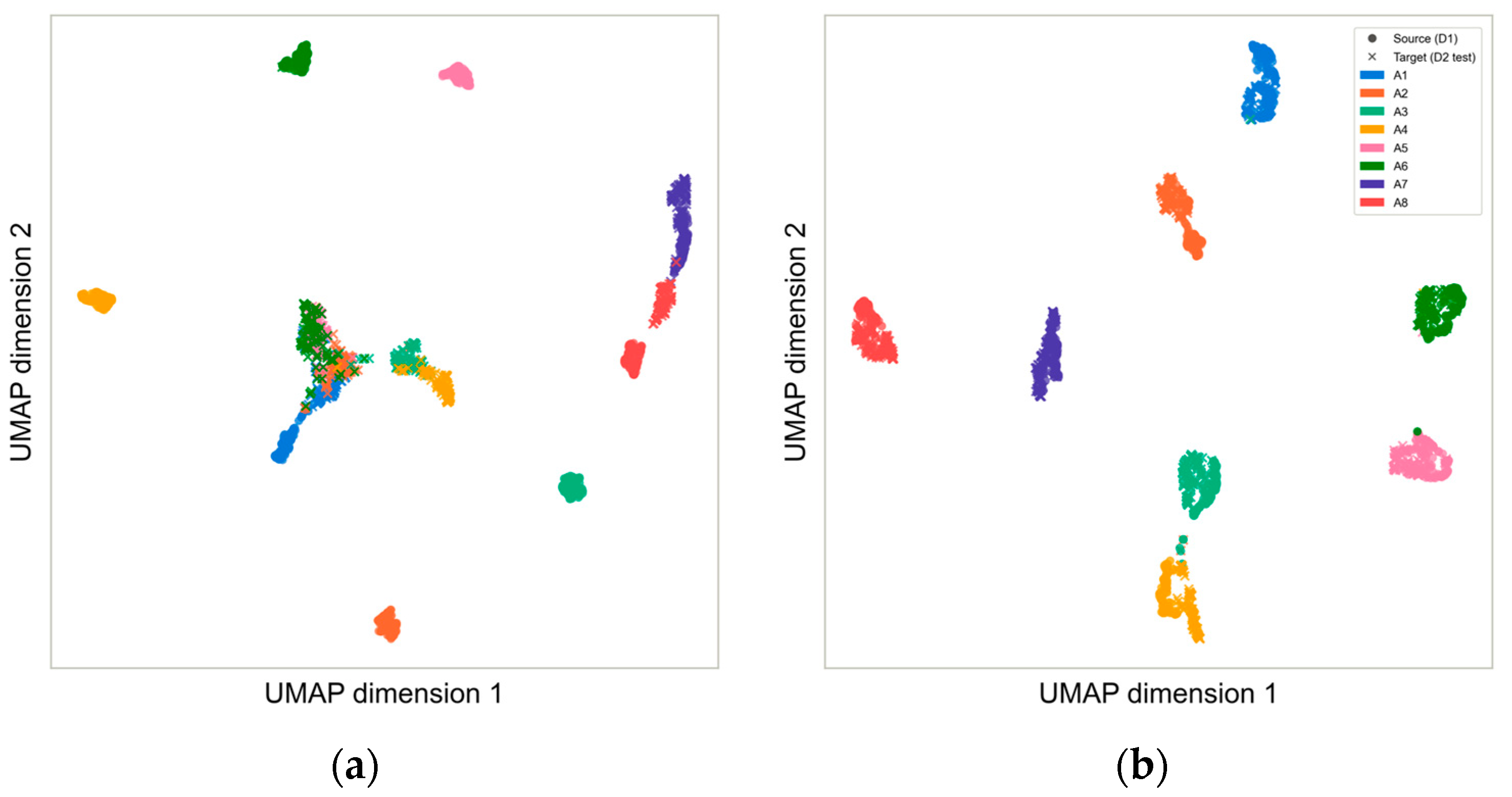
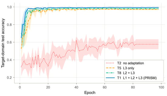
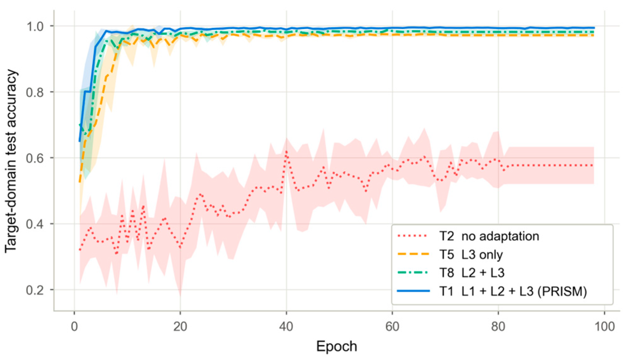
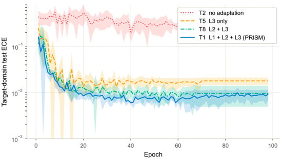
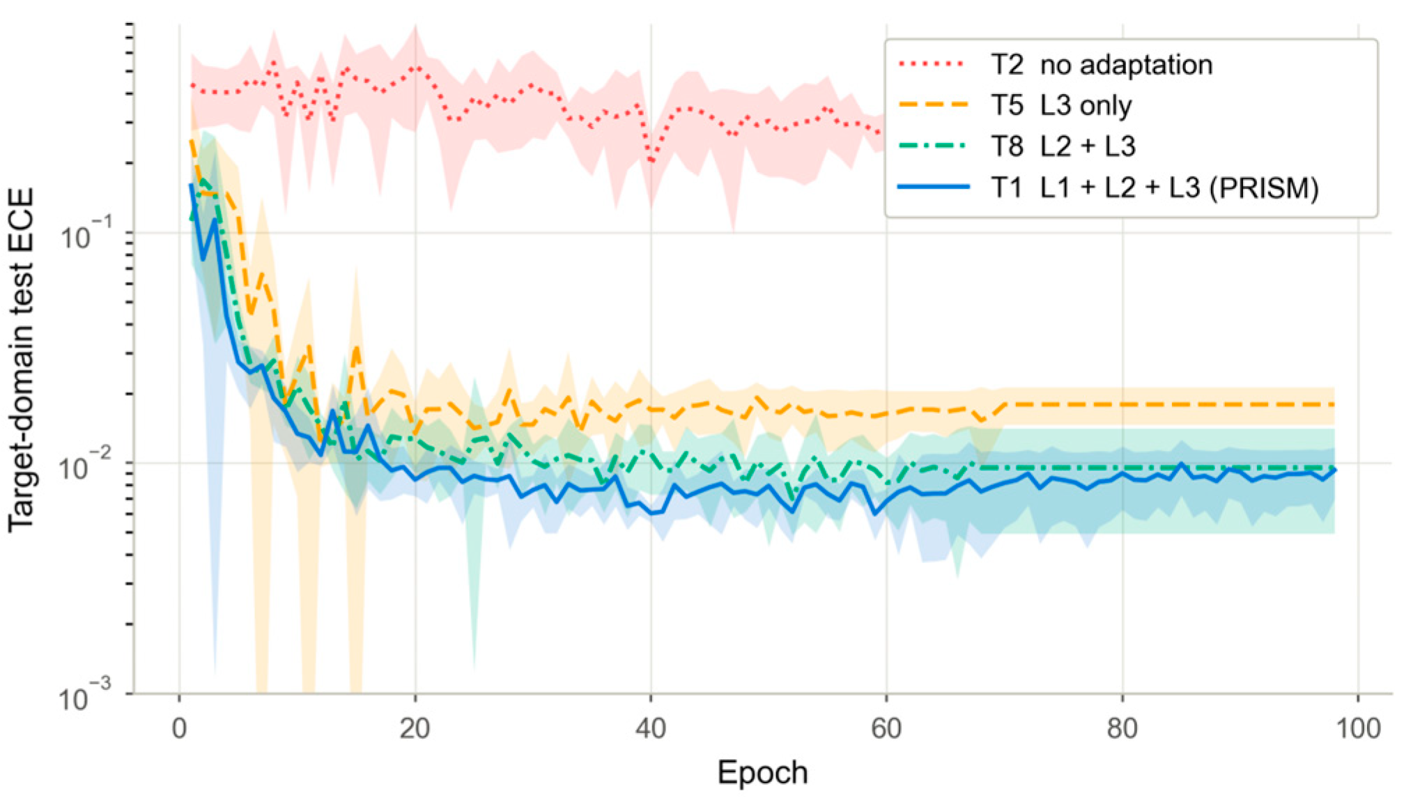

Disclaimer/Publisher’s Note: The statements, opinions and data contained in all publications are solely those of the individual author(s) and contributor(s) and not of MDPI and/or the editor(s). MDPI and/or the editor(s) disclaim responsibility for any injury to people or property resulting from any ideas, methods, instructions or products referred to in the content. |
© 2026 by the authors. Licensee MDPI, Basel, Switzerland. This article is an open access article distributed under the terms and conditions of the Creative Commons Attribution (CC BY) license.