


Abstract
Ground-based photometric data of high-orbit targets are essential for attitude estimation and physical characterization, but their quality is degraded by atmospheric turbulence, sky background, and tracking instabilities. Existing methods rely on discrete binary flags or statistical outlier rejection, lacking fine-grained credibility quantification and failing to exploit the physical prior of light curve smoothness. This paper proposes a quality assessment framework that replaces binary labels with continuous credibility scores. The method first segments data into continuous arcs, removes transient edge points, and extracts smooth trends. Then, three credibility factors (elevation angle, arc duration, and local residual robustness) are combined with hard rejection rules to yield a comprehensive score between 0 and 1. Daily and target-level scores are further synthesized for multi-granularity quality comparison. Experiments on real high-orbit photometric data show that the hard rejection ratio is below 3%, credibility distributions align well with observed data quality, and daily scores effectively distinguish good from poor observation nights. The generated credibility can be directly used as sample weights in downstream models, enhancing the reliability of optical data analysis.
1. Introduction
With the growing demand for space object surveillance, photometric data acquired from ground-based optical observations play an increasingly important role in areas such as attitude estimation, state discrimination, and behavioral analysis of space targets [1]. Light curves of high-orbit targets contain physical information about target size, attitude, and surface reflectance properties [2]; therefore, highly reliable photometric data are fundamental for retrieving target physical characteristics and training data-driven models.
However, in actual observations, the quality of photometric data is compromized by multiple interfering factors, including atmospheric turbulence [3], sky background [4], and equipment tracking stability [5]. If low-quality data are used indiscriminately, they may obscure critical dynamic features of satellites. Current ground-based photometric systems already provide second-level or even sub-second sampling capabilities [6], with single-night data volumes reaching tens of thousands of points, making manual point-by-point inspection impractical.
To address these issues, previous studies have explored various directions from different perspectives. At the level of data quality labeling, large-scale survey projects commonly adopt Data Quality Flags (DQF) systems [7], which encode instrumental anomalies such as pixel saturation, cosmic rays, and bad pixels via binary-bit flags. For example, in the ACS data quality arrays of the Hubble Space Telescope (HST), different numerical values correspond to different pixel issues [7]; the SDSS project classifies spectral plate-quality into three levels: “good”, “marginal”, and “bad” [8]; and the CALIFA survey defines quality control flags encompassing multiple parameters, including atmospheric quality and sky background [9]. In the realm of anomaly detection, statistical outlier rejection methods based on Sigma Clipping [10] are widely applied in light curve cleaning, iteratively removing outliers that exceed a certain standard deviation.
Nevertheless, data quality flags primarily label anomalies at the pixel and instrument levels, with outputs remaining discrete binary or multi-class labels. In practice, users ultimately have to convert these labels, through masking, into a simple “use” or “discard” decision—which is essentially still a hard classification, lacking fine-grained quantification of data-point credibility. Statistical methods like Sigma Clipping, on the other hand, rely on the distributional characteristics of the data themselves and fail to fully exploit the physical prior of light curve smoothness, which is intrinsically determined by the continuity of observational geometry.
For high-frequency photometric data of high-orbit targets, single-night observations can reach tens of thousands of points, making manual point-by-point inspection impractical. Moreover, downstream tasks such as magnitude estimation, attitude inversion, and anomaly detection require continuous sample weights rather than binary flags. Therefore, despite the existing methods described above, what is needed for high-frequency photometric data of high-orbit targets is a continuous, point-wise credibility score that can be directly used as a sample weight in downstream tasks. To the best of our knowledge, no such system has been reported for high-orbit targets. The main contribution of this work is therefore the development and validation of a continuous credibility scoring framework tailored to high-frequency photometric data of high-orbit targets. The proposed scores can be used as a quantitative basis for filtering high-quality observation arcs and targets, and their potential as continuous sample weights in downstream models is a direction for future work.
To this end, this paper proposes a quality assessment and credibility generation method tailored to high-frequency photometric data of high-orbit targets. The core idea is to construct a local trend baseline based on the physical prior of light curve smoothness, and to replace binary labels with continuous credibility for quality characterization. The specific procedure is as follows: first, the data are divided into continuous arcs according to observation time intervals; transient unstable points at the beginning and end of each arc are removed; and a smooth trend is extracted within each arc. Subsequently, continuous credibility factors are constructed for each data point from three dimensions—elevation angle, arc duration, and local residual robustness—and, combined with hard rejection rules, these yield a comprehensive credibility score between 0 and 1. On this basis, through multi-indicator weighted synthesis, comprehensive quality scores are generated for each target’s daily observations and for the overall dataset, with visual validation achieved via three-color scatter plots.
In summary, this paper presents a photometric data quality assessment framework that uses light curve smoothness as a physical prior. It upgrades discrete labels to continuous credibility and point-level to hierarchical scoring, and its outputs can be directly used in downstream tasks such as attitude inversion.
2. Data and Preprocessing
2.1. Data Sources and Format
The photometric data used in this work were obtained from the ground-based optical observation system of the National Astronomical Observatories, Chinese Academy of Sciences (NAOC). The telescope has a focal length of 150 mm, and the detector has a total pixel array of 4096 × 4118 with a pixel size of 9 μm. Other parameters, such as aperture, focal ratio, field of view, filters, and typical photometric accuracy, are not publicly available because of the data policy of the National Astronomical Observatories. The data sampling interval is non-uniform, with a sampling rate of approximately 1 Hz. Most of the observed targets are high-orbit space objects, and the photometry is performed using differential photometry—that is, by selecting one or more known stable reference stars within the same field of view and comparing the observed flux of the target star with that of the reference stars in real time [11]. This approach effectively removes common-mode errors such as atmospheric extinction and instrument response variations, yielding magnitudes with relatively high precision [12]. The differential photometry, including reference-star selection and uncertainty estimation, was performed by the observatory; the detailed procedures are not publicly available due to its data policy.
The raw records include: observation time (accurate to milliseconds), telescope pointing azimuth and elevation, raw magnitude, and normalized magnitude. The normalized magnitude is defined as the magnitude value after normalizing the target photometry to a phase angle of 90°. Data for the same target on the same day may be distributed across multiple files and must be merged during the preprocessing stage.
The overall dataset used in this study consists of 1382 targets, 26,731 observing nights summed over all targets, 69 distinct observing nights, 42,530 arcs, and 28,608,948 individual photometric measurements. The observations span 111 days from 1 January 2024 to 21 April 2024. The measured magnitudes range from 2.77 to 15.46 mag, and the telescope elevation angles range from 10.6° to 52.5°. On average, each target contains about 1070 measurements per observing night. The four targets (IDs: 25924, 32019, 41725, 43432) used for detailed visualization and analysis were randomly selected from this full dataset. A summary of the dataset is provided in Table 1.
Table 1.
Overview of the photometric dataset used in this study. “Observing nights (total)” is the sum of observing nights over all targets. “Distinct nights” is the number of different calendar dates. “Measurements” refers to individual photometric measurements. “Elevation range” is the telescope elevation angle range. Arcs are defined by a 30-min gap threshold.
2.2. Basic Data Characteristics and Preprocessing Workflow
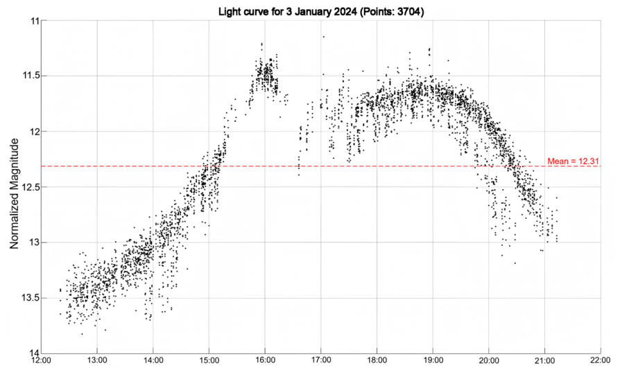
To rationally design the preprocessing pipeline, we must first clarify the core characteristics of this high-frequency photometric data. Compared with traditional photometric data, these 1-Hz high-frequency data exhibit three distinctive signal features, as illustrated in Figure 1: (1) Second-level magnitude fluctuations are approximately ±0.05–0.2 mag (based on our measured data). Because high-orbit targets are generally faint, these fluctuations arise from the combined contribution of readout noise [13], photon noise, and atmospheric scintillation; the relative contribution of photon noise increases toward the faint end. (2) The photometric variation of high-orbit targets is significantly influenced by the slow change in the Sun-target-station phase angle [14]. Over time spans of several hours, the phase angle typically varies smoothly, and the magnitude exhibits a gentle long-term trend. (3) The continuity of observation arcs varies. In some periods, owing to cloud cover, equipment adjustment, or the target entering or exiting Earth’s shadow, the data appear as multiple disjoint segments with inter-segment gaps ranging from half an hour to several hours.
Figure 1.
Scatter plot of normalized magnitude versus time for a typical target during one observing night. The x-axis indicates the observation time (UTC), and the y-axis represents the normalized magnitude (mag). The normalized magnitude has been calibrated via differential photometry to a fixed phase angle of 90°, effectively removing the dominant effects of atmospheric extinction and phase angle variations. Thus, the scatter plot reveals the target’s intrinsic brightness variations.
Based on the above data characteristics, we design the following standardized preprocessing pipeline:
- (1)
- Data aggregation and sorting
All record files are traversed to extract each field. The time information is combined into datetime objects and sorted in ascending order, forming a complete chronological observation sequence for the target.
- (2)
- Observation arc segmentation
A threshold of 30 min is used to divide continuous arcs; intervals exceeding this threshold are treated as separate arcs. This threshold is chosen empirically based on the characteristics of our observational data—half an hour is sufficient to distinguish long interruptions caused by equipment restarts or weather improvements, avoiding forced concatenation of non-continuous observations.
- (3)
- Trend smoothing and residual calculation
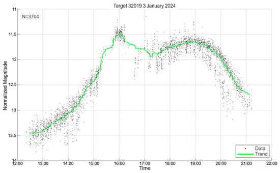
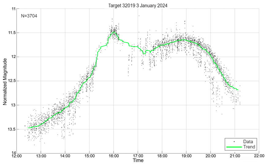
For the normalized magnitude sequence within each arc, a moving median filter with a window of 181 points (approximately 3 min) is applied [15]. The resulting smoothed value, mag_smooth, serves as the local trend baseline (see Figure 2.). The residual of each observation point relative to this baseline is then computed to characterize instantaneous deviations. The moving median uses a window of 181 points by default, which is reduced for shorter arcs and truncated near arc boundaries.
Figure 2.
Scatter plot and smoothing trend line of normalized magnitude for a typical observing arc. Black dots represent the normalized magnitude sampled at 1 Hz, and the green curve is the local trend line obtained by a moving median filter with a window of 181 points (approximately 3 min). This trend line effectively suppresses high-frequency fluctuations caused by atmospheric scintillation and detector readout noise, while preserving the true photometric trend induced by slow changes in target attitude or phase angle, thus providing a reliable local baseline for subsequent residual calculation.
The window width is chosen on the principle that it should effectively suppress the high-frequency random noise of 1-Hz sampling while preserving the true photometric trend induced by changes in target attitude or phase angle. After testing on multiple arcs, a window of 181 points was found to effectively filter out second-level scintillation and transient spikes, while stably tracking the local magnitude baseline, avoiding misclassifying genuine light curve details as noise.
After the above preprocessing, each observation record is augmented with four extended fields: Segment ID, Smoothed Mag, Residual, and Short Segment Flag. The data are organized hierarchically by target ID and date, forming a standardized data table (Table 2) for subsequent quality assessment and daily visualization.
Table 2.
Example of preprocessed high-frequency photometric data with extended fields.
2.3. Validation of the Smoothing Window: Injection–Recovery Test
The choice of the 181-point moving median window in Section 2.2 (3) is based on the requirement to suppress high-frequency noise while preserving the intrinsic photometric trend. However, GEO targets may exhibit short-timescale brightness variations due to rotation or tumbling, and it is essential to verify that the smoothing procedure does not misinterpret such real variability as noise.
To this end, we performed an injection–recovery test. This approach is widely used in time-domain astronomy to quantify the recovery efficiency of detection and analysis pipelines by inserting synthetic signals into real data and measuring the fraction that is recovered. In this work, the test was designed to assess whether the moving median window would suppress real periodic variations.
Published photometric studies of retired GEO satellites report rotation periods ranging from approximately 3 s to 1800 s. Most uncontrolled GEO satellites exhibit periods of 2–30 min (120–1800 s). Based on these observed ranges, we selected three representative periods for injection: 60 s (fast rotation), 120 s (transition regime), and 300 s (typical moderate rotation). This selection spans the range most likely to be affected by the 181-point window.
Sinusoidal modulations with amplitudes of 0.05, 0.10, and 0.20 mag were injected into the longest continuous arc of each target. The complete quality-assessment pipeline was then re-run. Three metrics were used to quantify the recovery performance: the hard rejection rate, the fraction of injected points that remain usable after quality assessment, and the mean comprehensive credibility. The precise definitions of these metrics are given in Section 3.3.
The results, presented in Section 5.1, demonstrate that the hard rejection rate remained below 1% for all injected periods and amplitudes, and the vast majority of the injected points were retained by the quality assessment. This indicates that, under the tested conditions, the selected smoothing window does not hard-reject the injected sinusoidal signals; it only down-weights points that deviate from the local trend without discarding them. A detailed quantitative analysis is given in Section 5.1.
3. Quality Assessment Methodology
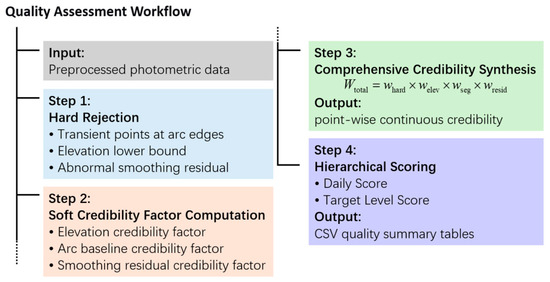
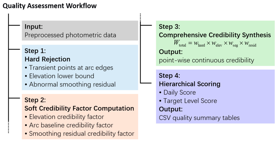
The core of our quality assessment is not to classify data points as binary “good/bad” labels but to assign each observation a continuous, comprehensive credibility score between 0 and 1, quantitatively characterizing its reliability. The assessment is conducted along three independent dimensions: observation elevation angle, arc duration, and local smoothing residual. In implementation, we adopt a “hard rejection + soft credibility factor” strategy: first, obviously unreliable points are removed using explicit thresholds; then, for the remaining points, continuous credibility values are assigned according to the degree of deviation in each dimension. The overall quality assessment workflow is shown in Figure 3.
Figure 3.
Flowchart of the proposed quality assessment and scoring framework. Step 1: hard rejection; Step 2: soft credibility factor computation; Step 3: comprehensive credibility synthesis; Step 4: hierarchical scoring.
3.1. Hard Rejection Conditions
Hard rejection targets points that are clearly anomalous or at physical limits, directly assigning a credibility of 0 and excluding them from subsequent analysis. The threshold for each condition was determined based on statistical principles, physical priors, and the actual data distribution, and was experimentally verified and fine-tuned. The hard rejection stage applies three criteria: (i) the first and last 10 points of each arc, among which those with residuals exceeding the threshold are removed; (ii) elevation below 20°; and (iii) absolute smoothing residual above 1.0 mag.
3.1.1. Transient Points at Arc Ends
Under conditions such as low-speed tracking, the telescope servo system typically requires a settling time of several seconds up to about 8 s from startup to stable tracking [16]. At the end of an observation, the target may be lost due to westward setting or programmed termination, leading to loss of lock or deceleration. Therefore, data at the beginning and end of arcs are nonstationary outliers and should be subjected to stricter screening. Specifically, we select the first and last 10 points of each arc (approximately 10 s) and remove those with residuals exceeding σ. Throughout this section, the residual standard deviation σ is defined as the robust standard deviation of the residuals within each arc, computed as σ = 1.4826 × MAD, where MAD is the median absolute deviation. The detailed formulation is given in Section 3.2.3. A length of 10 s is slightly longer than the typical settling time, covering transient effects while avoiding excessive penalization of valid data. If an arc contains fewer than 20 points, the end-point screening cannot be reliably performed, and the entire arc is marked as a short segment and hard-rejected, because such short arcs lack sufficient data for local trend estimation and contain negligible phase angle variation.
3.1.2. Elevation Lower Bound
Although differential photometry can cancel first-order atmospheric extinction, low elevation angles still introduce residual errors [17]. Referring to the quality control strategy of the CALIFA survey, we treat an air mass exceeding 2.0 (corresponding to elevation <30°) as a warning condition [9]. In our measured data, points with elevation below 20° are extremely rare; hence we set 20° as the hard lower bound. Points between 20° and 30° are softly down-weighted via a credibility factor (Section 3.2.1) to retain marginal but still useful data.
3.1.3. Abnormal Smoothing Residual
In the preprocessing stage, a moving median filter has been applied to the normalized magnitude sequence of each arc to obtain a local smoothed trend line. The smoothing residual at each point is defined as the difference between the normalized magnitude and its smoothed value at that point, reflecting the instantaneous deviation of the point from the local average trend.
In the light curves of high-orbit targets, photometric variation is slowly modulated by the observation geometry, even when specular reflections are taken into account; jumps exceeding 1 mag within seconds are generally not expected. The 1 mag threshold for rejecting extreme outliers has also been adopted in previous photometric studies in other fields [18], and is used here as a reference. Accordingly, we set the threshold such that points with an absolute smoothing residual exceeding 1.0 mag are considered to be subject to transient interference and are consequently rejected.
The above three hard rejection rules collectively eliminate approximately 3% of the total data points (depending on actual data), providing a clean baseline for subsequent soft credibility factor computation.
3.2. Design of Soft Credibility Factors
For observation points that survive hard rejection, soft weight factors between 0 and 1 are computed from three dimensions. The product of these factors yields the comprehensive credibility, enabling models or analysis algorithms to perceive data quality from multiple aspects.
3.2.1. Elevation Credibility Factor welev
As noted in Section 3.1.2, low elevation introduces residual atmospheric effects and mechanical instability, so data at low elevation should be moderately penalized. We design the elevation weight as a piecewise linear function, as shown in Equation (1):
where welev denotes the elevation credibility factor, and elev denotes the elevation angle of the point.
Points below 20° have already been removed by the hard rejection stage, so the soft elevation factor is set to 0 in this range to keep the boundary conditions mathematically consistent. Between 20° and 30°, the weight transitions linearly to 1, achieving a soft downweighting. Above 30°, the data are fully trusted. This strategy suppresses the uncertainty at low elevations while retaining potentially valuable information under marginal conditions.
3.2.2. Arc Baseline Credibility Factor wseg
The photometric variation of high-orbit targets is slowly modulated by observation geometry. Longer arcs provide broader phase angle coverage, which is more favorable for characterizing the phase-magnitude relationship; extremely short arcs contain only isolated magnitude values and lack geometric variation information, offering limited modeling value. Accordingly, we introduce the arc-baseline credibility wseg, obtained as the product of duration credibility and point-count credibility, as shown in Equation (2), shared by all points within the arc:
where Tseg is the arc duration (in seconds) and Nseg is the number of points within the arc.
There is no universally accepted standard in the open literature for the minimum arc length of high-orbit targets. Referring to the geometric information requirements and accuracy trust for initial orbit determination [19], and considering the 1-Hz sampling density of our data, we set Tref = 600 s and Nmin = 580 as full-score thresholds. Arcs meeting these criteria receive full credibility in this dimension; otherwise, the factor decays proportionally, reflecting the reduced information content of short arcs.
3.2.3. Smoothing Residual Credibility Factor wresid
Under normal observing conditions, the normalized magnitude of a target should vary smoothly. Some studies have pointed out that specular reflections (“flashes”) from solar panels of GEO satellites have strict geometric window constraints; each station globally can observe them in only two periods per year, about 32 min per day [20]. Therefore, such transient events can be neglected in most routine observation sessions. Consequently, points that deviate significantly from the local trend are highly likely to be affected by instantaneous disturbances; penalizing residuals can effectively suppress occasional anomalies.
Specifically, for each arc, we compute the robust standard deviation of the residuals σ = 1.4826 × MAD [21] and define the normalized deviation z = |residual|/σ. The credibility function is a piecewise linear function [22], as shown in Equation (3):
where k1 = 1.0, k2 = 3.0. That is, residuals within σ are considered normal fluctuations and receive full credibility; beyond σ, linear down-weighting begins, reaching zero at 3σ.
The thresholds k1 = 1.0 and k2 = 3.0 are more conservative (stricter) than the commonly used 2σ/4σ criterion. Because the residuals after moving-median smoothing are not strictly Gaussian and the local signal-to-noise ratio varies across arcs, a tighter inner threshold provides a finer down-weighting gradient for marginal points. A sensitivity analysis shows that replacing these thresholds with 1.5σ/3.5σ or 2σ/4σ changes the target ranking only marginally, with Spearman ρ = 0.988 and 0.976, respectively. The detailed results are presented in Section 5.2.
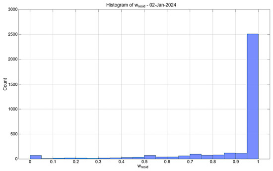
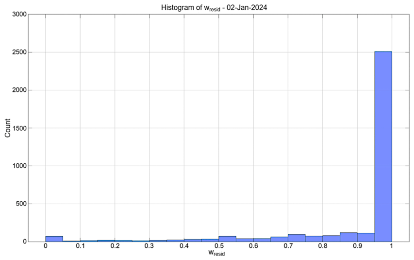
This relative threshold complements the absolute 1.0 mag hard rejection threshold: the latter captures physically implausible jumps of extremely large amplitude, while the relative threshold targets local statistical anomalies within the arc. For points where the residual is undefined (e.g., NaN in very short arcs), we assign wresid = 0.5. The rationale is not that 0.5 is a midpoint, but that no information is available to judge whether such a point is good or bad. Assigning 0 or 1 would introduce a systematic bias: 0 would penalize a point without evidence of a defect, while 1 would fully trust a point without evidence of quality. A value of 0.5 represents a maximum uncertainty or uninformative prior, which is a standard choice in missing-data management [23]. These points are rare; their overall contribution to the credibility distribution is therefore limited. The final effect is shown in Figure 4.
Figure 4.
Histogram of residual weight (wresid) distribution for a typical observation arc. The x-axis shows the weight value (computed from a truncated linear decay of normalized magnitude residuals), and the y-axis is the count of visits per bin.
3.3. Comprehensive Credibility Synthesis Wtotal
The comprehensive credibility Wtotal for each observation point is the product of the hard rejection flag and the three soft credibility factors, as shown in Equation (4):
where whard ∈ {0,1} is the hard rejection flag (1 for retained, 0 for rejected).
Wtotal = whard × welev × wseg × wresid
The multiplicative combination is adopted because quality assessment inherently requires that a data point satisfy credibility conditions in all dimensions simultaneously: if any dimension exhibits a severe defect, the corresponding factor approaches zero, and the comprehensive credibility is correspondingly reduced or nullified. The product operation naturally embodies this “bottleneck effect.” Each factor lies between 0 and 1, so Wtotal ∈ [0,1], and it can be directly used as sample credibility in subsequent modeling. For the vast majority of points that survive hard rejection, the comprehensive credibility is predominantly distributed between 0.6 and 1.0, forming a “soft-filtered” high-quality dataset.
4. Scoring System Construction
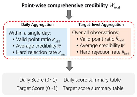
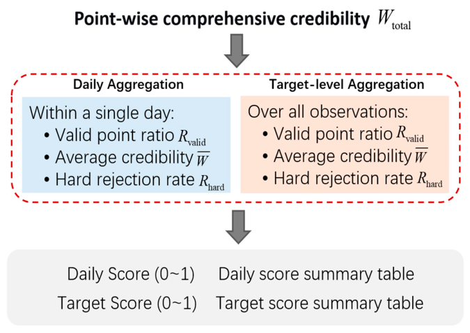
The point-level comprehensive credibility Wtotal generated in Section 3.3 finely characterizes the credibility of each observation point. However, in practical tasks, researchers often need a quick assessment of the overall data quality for an entire day or for a whole target. Therefore, based on the point-level weights, we further designed a two-level scoring system—daily score and target score—as illustrated in Figure 5.
Figure 5.
Two-level scoring framework.
4.1. Scoring Metrics and Comprehensive Score Formulation
We characterize the quality profile of an observation set (one day or one target) from three perspectives:
- Valid point ratio Rvalid: the proportion of points with comprehensive credibility Wtotal > 0.3, reflecting the coverage of “basically usable” points.
- Average comprehensive credibility : the arithmetic mean of comprehensive credibility Wtotal over all data points, reflecting the overall credibility of the dataset.
- Hard rejection rate Rhard: the proportion of points that are hard rejected (Wtotal = 0), directly indicating the degree of data contamination.
These three metrics answer the core questions “how much data are usable”, “how reliable are the data overall”, and “how much data are corrupted”, respectively, and collectively provide a comprehensive description of data quality.
After normalizing the above three indicators to the same scale, we used a weighted linear combination to obtain a comprehensive score in [0,1]. For an observation set (daily or target), the score S is defined as Equation (5):
where α, β, γ are weight coefficients satisfying α + β + γ = 1.
Based on the importance of each indicator, we select α = 0.4, β = 0.4, γ = 0.2, placing more emphasis on the valid point ratio and average credibility, while the hard rejection rate serves as a warning without excessive penalty. The rationale is that the average credibility and valid point ratio are core measures of data quality and should be equally weighted (0.4 each); the hard rejection rate is already indirectly reflected in the valid point ratio, and including it as a separate term only enhances sensitivity to severe contamination, so a modest weight of 0.2 is appropriate. When all points are highly credible and no hard rejection occurs, S approaches 1; otherwise, S decreases significantly.
4.2. Hierarchical Quality Scores: Daily and Target-Level
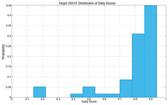
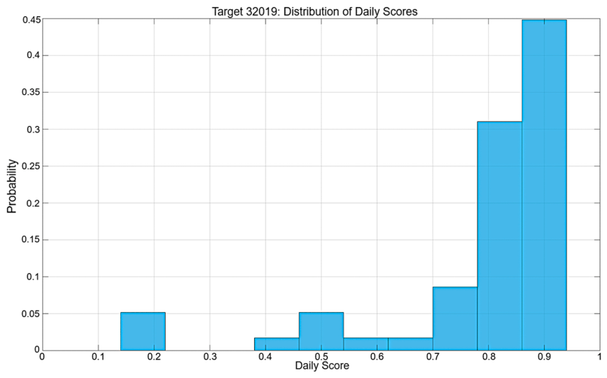
The same composite scoring (Equation (5)) is applied at two aggregation levels. At the daily level, all observation points within a single calendar day are used to compute the three indicators–valid point ratio Rvalid, average comprehensive credibility , and hard rejection rate Rhard—which are then substituted into Equation (5) to yield the daily score Sday. These daily scores enable rapid identification of high-quality observation nights (e.g., retaining days with Sday > 0.6 for further analysis). At the target level, we aggregate all observation points across all available days for a given target, recompute the same three indicators over the entire target dataset, and obtain the target-level score Stgt. This higher-level score reflects the cumulative long-term data quality for each target and facilitates horizontal comparisons among different targets. To present both hierarchies compactly, we combine the daily and target-level statistics into a single Table 3. The distribution of daily scores is also visualized in Figure 6, where the area under the curve is normalized to unity.
Table 3.
Hierarchical quality scores: daily and target-level. The table lists for each target and each observation day (or target total) the total point count, valid point ratio, average/median weight, hard rejection ratio, low-weight ratio, and the corresponding composite score. The median weight is the median value of Wtotal over all points in the observation set. The low-weight ratio is the proportion of points with Wtotal ≤ 0.3.
Figure 6.
Probability density histogram of daily scores. The horizontal axis shows the daily score (range 0–1), and the vertical axis indicates probability density. The histogram is normalized so that the total area under the bars equals 1, illustrating the relative frequency of different daily score bins across all observation days.
The two-level scoring system, together with the point-level comprehensive credibility, constitutes a hierarchical data quality product. In practical use, users can: (1) quickly filter out targets with very poor quality using the target-level score; (2) select high-credibility observation arcs using the daily score; and (3) within selected arcs, use the point-wise comprehensive credibility as sample weights in model training. Preliminary visual inspection suggests that the scoring results are consistent with the observed data quality trends.
5. Experiments and Performance Evaluation
To validate the effectiveness of the proposed quality assessment method, we processed real photometric data from multiple high-orbit targets. From the processed targets, we randomly selected four (IDs: 25924, 32019, 41725, 43432) to demonstrate the visualization effect, credibility distribution, and scoring ranking capability, providing both quantitative and qualitative analyses of the method’s performance.
5.1. Injection–Recovery Test Results
To verify that the selected smoothing window does not remove real short-timescale variability, we performed an injection–recovery test on four GEO targets (IDs: 25924, 32019, 41725, 43432). Sinusoidal modulations with periods of 60, 120, and 300 s and amplitudes of 0.05, 0.10, and 0.20 mag were injected into the longest continuous arc of each target. The full quality-assessment pipeline was then re-run, and three metrics were recorded: the hard rejection rate, the valid point ratio (defined as the fraction of points with Wtotal ≥ 0.3), and the mean comprehensive credibility .
Table 4 summarizes the results at the largest injected amplitude of 0.20 mag, which represents the most challenging case. Across all targets and periods, the hard rejection rate remained below 1%, and the valid point ratio exceeded 85%. Even for the shortest period of 60 s, which is much shorter than the 181-point window (approximately 181 s), the valid point ratio remained above 85%. As the injected amplitude increases and the period decreases, the valid point ratio shows a slight decrease, but the hard rejection rate remains negligible. This trend is expected: larger and faster variations are more likely to deviate from the local trend and thus receive lower credibility weights, but they are not removed. This confirms that the smoothing procedure down-weights, rather than discards, real short-timescale variability.
Table 4.
Injection–recovery test results for the four GEO targets at the largest injected amplitude of 0.20 mag. A sinusoidal modulation is injected into the longest continuous arc of each target. The test is performed for injected periods of 60, 120, and 300 s.
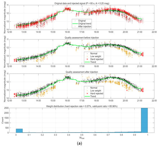
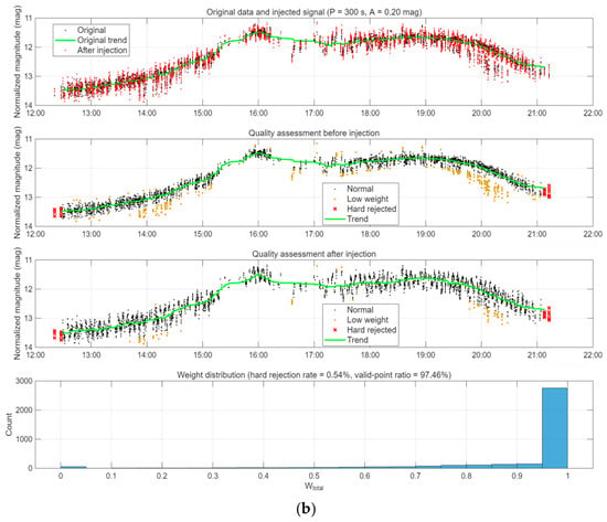
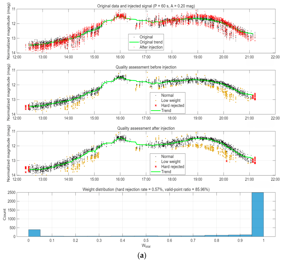
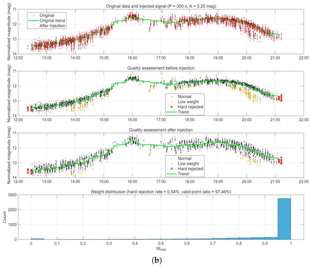
Figure 7 presents two representative injection–recovery cases at the largest injected amplitude of 0.20 mag for target 32019: (a) P = 60 s, which is much shorter than the 181-point window (approximately 181 s at 1 Hz sampling) and thus represents the most challenging case; and (b) P = 300 s, which is longer than the window and represents the typical rotation period of uncontrolled GEO satellites. In each case, the four panels show, from top to bottom: the original light curve with the injected signal; the quality assessment before injection; the quality assessment after injection; and the distribution of Wtotal. For the 60 s case, the vast majority of injected points remain normal (black), with only a few low-weight points (yellow) and almost no hard-rejected points (red crosses), and the distribution of Wtotal peaks near 1.0. For the 300 s case, the trend baseline is able to partially follow the injected variation, and the quality labels remain similarly benign. In both cases, the hard rejection rate stays below 1%. The difference between the two cases can be understood from the ratio of the injected period to the smoothing window. For the 60 s case, the period is about one third of the window, so the moving median spans about three full cycles and tends to average out the oscillation rather than follow it; the injected signal therefore remains largely in the residual, leading to a higher degree of down-weighting. For the 300 s case, the period is longer than the window, so the moving median can partially track the variation and absorb it into the trend baseline, leaving less signal in the residual and causing less down-weighting. This explains why the valid point ratio is lower for 60 s and higher for 300 s, while the hard rejection rate remains negligible in both cases. These results confirm that the smoothing procedure down-weights, rather than removes, short-timescale variations that deviate from the local trend.
Figure 7.
Injection–recovery test at the largest injected amplitude of 0.20 mag. (a) P = 60 s, the most challenging case, where the injected period is much shorter than the 181-point window; (b) P = 300 s, the typical case, where the injected period is longer than the window. In each panel, the four subplots show the original and injected light curves, the quality assessment before injection, the quality assessment after injection, and the distribution of Wtotal.
In summary, the injection-recovery test demonstrates that, under the tested conditions, the 181-point moving median window does not hard-reject injected sinusoidal signals with amplitudes up to 0.20 mag and periods down to 60 s. Generalization to real rotational or tumbling signals requires further validation.
5.2. Sensitivity Analysis
To evaluate the robustness of the proposed scoring system, we performed a sensitivity analysis on five key parameters: the residual thresholds k1, k2, the smoothing window length, the scoring weights α, β, γ, the arc-baseline parameters Tref, Nmin, and the arc-segmentation threshold. Ten targets were randomly selected from the dataset for this analysis. Each parameter was varied over a reasonable range while the others were held fixed at the values adopted in this study. For each setting, the target-level score was computed for all ten targets, and the resulting ranking was compared with the baseline ranking using Spearman’s rank correlation coefficient ρ.
The parameter settings are summarized as follows. The residual thresholds k1, k2 were varied from the values adopted in this study (1.0, 3.0) to (1.5, 3.5) and (2.0, 4.0). The smoothing window length was varied from 181 points to 121 and 241 points. The scoring weights α, β, and γ were varied from the values adopted in this study, (0.4, 0.4, 0.2), to (0.3, 0.5, 0.2) and (0.5, 0.3, 0.2). The arc-baseline parameters Tref, Nmin were varied from the values adopted in this study, (600, 580), to (400, 400) and (800, 760). The arc-segmentation threshold was varied from 30 min to 15 and 45 min.
As shown in Table 5, all Spearman correlation coefficients are 0.976 or higher. The residual thresholds k1, k2 and the scoring weights α, β, γ produce slightly lower correlations of 0.976–0.988, which still indicate a highly consistent ranking. For the smoothing window, the arc-baseline parameters Tref, Nmin, and the arc-segmentation threshold, the rankings are essentially unchanged (ρ ≥ 0.997). These results confirm that the target ranking is robust to variations in all tested parameters. It should be noted that Spearman’s rank correlation coefficient measures the consistency of the relative ordering of targets, not the stability of the absolute score values. The absolute credibility scores may shift slightly when parameters are varied, but the relative quality stratification among targets remains unchanged. The main conclusions therefore do not depend on fine-tuning of these parameters.
Table 5.
Sensitivity analysis of key parameters. Spearman’s rank correlation coefficient ρ between the rankings of target-level scores under the baseline and perturbed settings. The baseline values are those adopted in this study. Ten targets were randomly selected for the analysis.
In addition to parameter sensitivity, we examined whether the target ranking depends on the choice of the combination method for the soft credibility factors. The product form used in this study was compared with three alternatives: an equal-weight weighted sum, a geometric mean, and the minimum. Using the same ten randomly selected targets, the target-level scores were recomputed under each combination, and the resulting rankings were compared with the product method using Spearman’s rank correlation coefficient ρ. As shown in Table 6, all three alternatives yield ρ = 1.000, indicating that the target ranking is completely insensitive to the choice of combination. The absolute scores may shift slightly, but the relative ordering and the main conclusions remain unchanged.
Table 6.
Sensitivity of the target ranking to the combination method. Spearman’s rank correlation coefficient ρ between the product method and three alternative combinations, computed on ten randomly selected targets.
5.3. Visual Validation
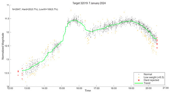
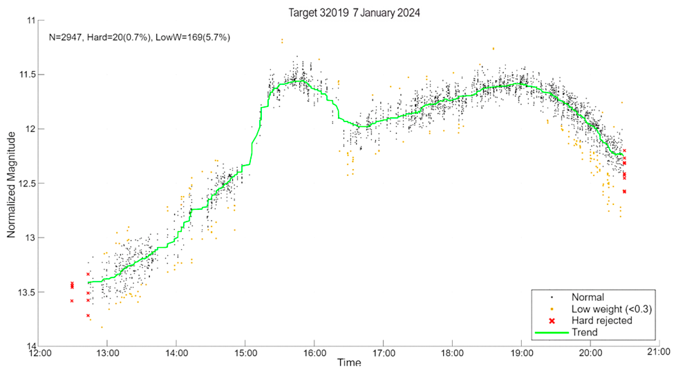
In the absence of expert-labeled data, three-color scatter plots are used as a visual validation tool to inspect the consistency between the assigned credibility weights and the observed data quality, as shown in Figure 8. In the plot, black points represent normal points (Wtotal ≥ 0.3 and whard = 1), yellow points denote attention points that are down-weighted but not rejected (Wtotal < 0.3 and whard = 1), and red crosses indicate hard-rejected points (whard = 0); the green curve is the smoothed trend line. The visualization allows immediate observation of the locations of hard-rejected points, the distribution of low-weight attention points, and the reasonableness of the trend line.
Figure 8.
Quality-labeled three-color scatter plot for a typical observing arc. Taking one day of observation for a target as an example, the plot clearly shows that hard-rejected points are mostly located at transient edges of arcs or isolated jumping points, while low-weight points often appear in short segments where the local signal-to-noise ratio is slightly lower, although the overall trend remains well defined. Most black points in continuous arcs closely follow the green trend line, demonstrating that the smoothing preserves the intrinsic photometric variation. This visualization method provides a convenient visual support for daily data quality assessment.
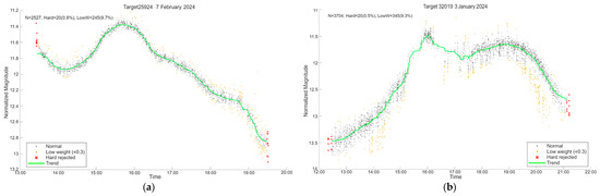
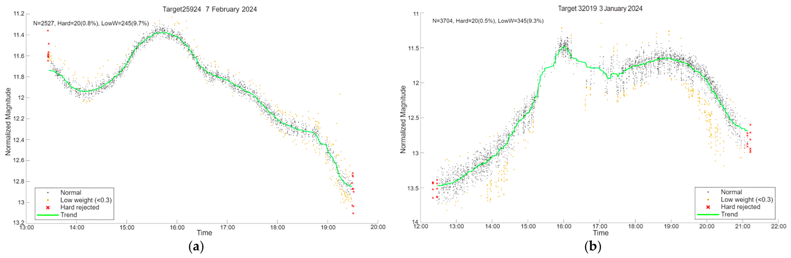
For routine high-quality observation days (Figure 9a,b), the normalized magnitudes closely follow the trend line, arcs are continuous and complete, and only the beginning and end points are marked as rejected due to transient tracking effects. The vast majority of points are black high-confidence points, with only a few yellow attention points. This indicates that under good observing conditions, our method is sufficiently tolerant of normal measurement fluctuations and almost never causes false rejections.
Figure 9.
Quality labeling distribution for routine high-quality observation days: (a) target 25924 (7 February 2024); (b) target 32019 (3 January 2024).
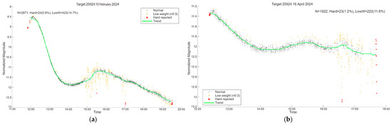
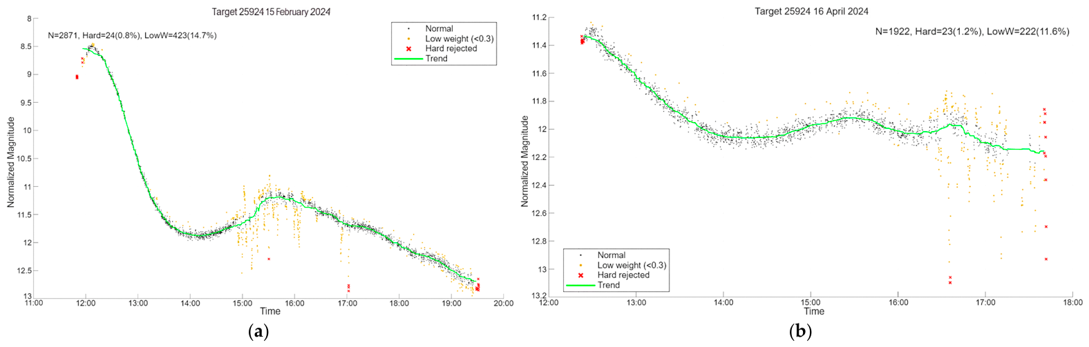
For days with local deviations (Figure 10a,b), the overall arc remains continuous, but in some periods, magnitude values deviate significantly from the trend line, showing notable fluctuations. These deviating points are marked as yellow attention points, accurately delineating intervals with slightly lower data consistency. Within the normal regions, points are still predominantly black high-confidence points; the red rejection markers in the middle of arcs correspond exactly to locations where magnitude values exhibit abrupt jumps. This validates the effectiveness of the comprehensive credibility in outlier detection: it can effectively flag local anomalies without affecting the overall high-credibility data segments.
Figure 10.
Quality labeling distribution for observation days with local trend deviations: (a) target 25924 (15 February 2024); (b) target 25924 (16 April 2024).
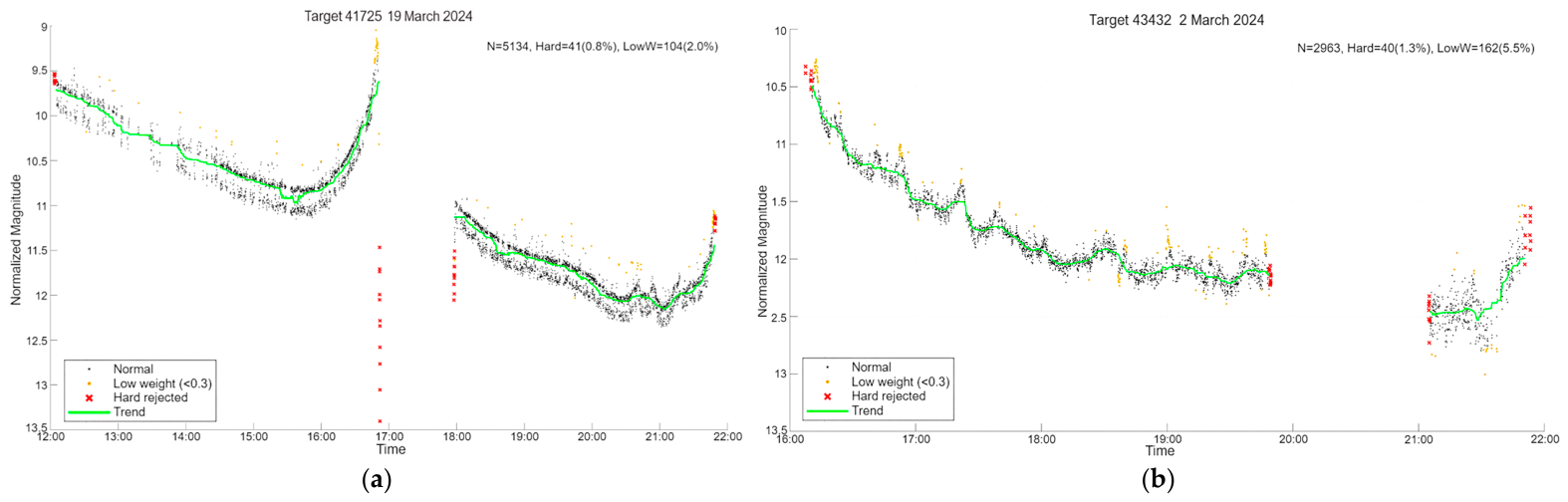
For days with fragmented arcs (Figure 11a,b), the data are split into multiple independent arcs due to equipment adjustments or cloud cover. The algorithm automatically identifies and removes the first and last 10 points of each arc, with the rejection markers located at both ends of each segment, confirming the effective triggering and execution of the edge-rejection strategy.
Figure 11.
Quality labeling distribution for observation days with fragmented arcs: (a) target 41725 (19 March 2024); (b) target 43432 (2 March 2024).
5.4. Credibility Distribution and Statistics
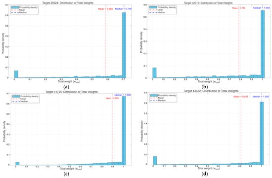
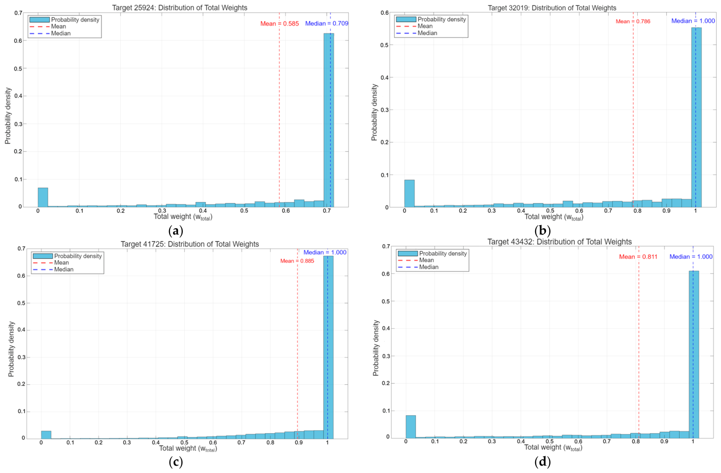
To examine the overall distribution characteristics of the comprehensive credibility, we performed a quality assessment on the observation data of the four targets, obtaining probability density histograms of the comprehensive credibility (Figure 12).
Figure 12.
Histograms of target comprehensive credibility distributions. (a–d) correspond to Target ID 25924, 32019, 41725, and 43432, respectively. The horizontal axis shows the total weight of comprehensive credibility (range 0–1), and the vertical axis indicates probability density. The histogram is normalized so that the total area under the bars equals 1, illustrating the relative frequency of observation points across different credibility bins for all four targets. In each subplot, the red dashed line marks the mean and the blue dashed line marks the median.
As can be seen from the figures, the credibility distributions of the four targets are highly consistent: all exhibit a typical unimodal left-skewed shape, with the main peak concentrated in the high-credibility range and a gentle long tail extending toward the low-credibility direction. The distribution peaks of three targets fall within the 0.9–1.0 interval, indicating that the vast majority of observation points are at a reliable level; the peak of the remaining target is located near 0.7, with slightly lower overall credibility (which is also consistent with the lower score of this target in Table 3), while the distribution structure and variation pattern remain consistent with the previous three targets. The proportion of samples with comprehensive credibility below 0.3 is very small, mostly corresponding to observation scenarios susceptible to interference, such as arc edges, isolated jumps, or short arcs, indicating that the overall quality of the observational data is good, without widespread contamination.
The median credibility of each target lies in the high-value range of the distribution, as shown in Figure 12. Although the mean credibility varies among targets, their distribution shapes (skewness and kurtosis) remain essentially consistent, with the main peak stably concentrated in the high-credibility range. This consistency holds across targets with different brightness, demonstrating the robustness of our method. The comprehensive credibility is computed from local distributional features, including the smoothing residual, the arc information content, and the elevation angle, so that it can objectively reflect the intrinsic quality of each individual observation point.
The above statistical results demonstrate that, while retaining the full data sample, our method achieves fine-grained differentiation among observation points of different credibility levels: high-credibility samples cluster in the core interval, forming the main body of the dataset; the few disturbed samples, after soft down-weighting, are still retained, avoiding the information loss that would result from a “one-size-fits-all” hard rejection. This differentiated credibility distribution provides a reliable basis for credibility-weighted fitting in subsequent model training.
5.5. Effectiveness of the Scoring System
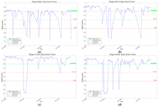
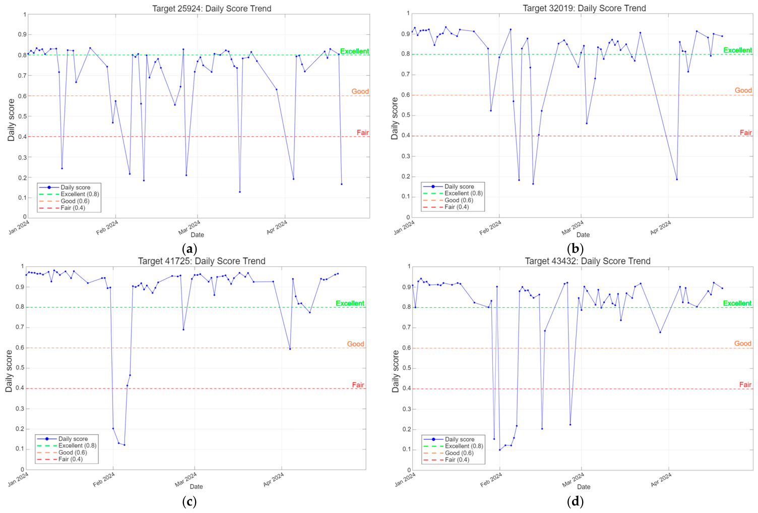
The daily score effectively distinguishes data quality across different days. Figure 13. shows line plots of daily scores for the four targets over multiple observation days, with three horizontal reference lines marking quality levels.
Figure 13.
Line plots of daily score variations for each target. (a–d) correspond to Target 25924, 32019, 41725, and 43432, respectively. In each subplot, the horizontal axis shows the observation date, and the vertical axis indicates the daily score (range 0–1). The blue line with markers represents the daily score, and the green, orange, and red dashed lines mark the reference quality thresholds for “Excellent” (0.8), “Good” (0.6), and “Fair” (0.4), respectively. These thresholds are operational and are intended for rapid screening of observation days; they are not derived from an external quality classification standard.
As seen in the figures, the daily scores for the same target show noticeable fluctuations across different days, reflecting variations in observing conditions and data quality. Between different targets, the overall distribution of daily scores also differs—some targets have scores concentrated in the excellent range, while others have lower scores with greater variability. This cross-day and cross-target discriminative ability makes the daily score a quantitative basis for automatically selecting high-quality arcs: for example, setting a threshold of 0.6 would retain only days rated Good or above for subsequent analysis. The target-level score provides an intuitive metric for horizontal comparison among multiple targets, facilitating the prioritization of targets with higher data quality.
5.6. Ablation Study: Effect of Sample Filtering Strategies on Magnitude Prediction
To evaluate the performance of the proposed quality assessment method Wtotal in actual training, we compared three sample filtering strategies: (1) no filtering (NF), (2) sigma clipping (SC), and (3) the proposed credibility-based filtering (CF). NF uses all samples for training and testing without any filtering. SC applies iterative σ clipping to the moving-median smoothing residuals, with two thresholds, 3σ and 2.5σ, where 3σ is a commonly used default in the literature and 2.5σ is a more aggressive filtering setting. CF uses the point-wise comprehensive quality weight Wtotal proposed in this paper and removes a fixed proportion (15% in this study) of the lowest-quality samples via a quantile threshold. This proportion is used as an illustrative example to demonstrate the filtering strategy and is not a tuned parameter. The threshold can be adjusted according to the requirements of specific downstream tasks. A systematic sensitivity analysis of different quantiles is left for future work.
The downstream prediction model is a multilayer perceptron (MLP) with an 8-dimensional input layer, two hidden layers of 30 neurons each, and a 1-dimensional output layer for magnitude prediction. The 8 input features consist of the unit vector of the Sun (3 dimensions), the unit vector of the target (3 dimensions), and the sine and cosine of the phase angle (2 dimensions). Training was performed using the fitrnet function in MATLAB with its default settings. For each method, a random 80/20 training/testing split was performed independently at the level of individual photometric points with a fixed random seed of 42. Because 1 Hz measurements within the same arc are correlated, this point-wise split may introduce some information leakage between the training and test sets. However, all three filtering strategies used exactly the same split, so the relative comparison among them remains fair. Splitting by observation arc would be more rigorous and is left for future work. The test set did not participate in any filtering, standardization, or normalization statistics. The evaluation metrics were RMSE and MAE on the test set, in magnitudes.
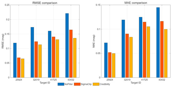
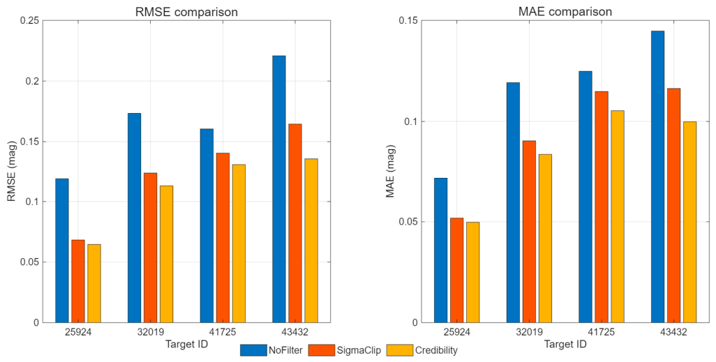
Table 7 presents the quantitative results for four targets. NF serves as the baseline. SC, with either the 3σ or 2.5σ threshold, reduces the RMSE compared with NF, indicating that removing residual outliers improves prediction accuracy. The proposed CF achieves the lowest RMSE and MAE among all strategies. For example, for target 25924, CF yields an RMSE of 0.0646 mag and an MAE of 0.0497 mag, which are lower than those of SC at both thresholds. This demonstrates that the filtering strategy based on multi-dimensional quality scores outperforms iterative clipping that relies solely on residuals. The RMSE and MAE comparisons for the four targets are presented in Figure 14. Furthermore, the CF threshold directly corresponds to the sample retention ratio, which has clear operational significance and can be readily adjusted according to the requirements of specific downstream tasks. It requires only a single quantile calculation without iteration, making it more flexible and interpretable in practical deployment.
Table 7.
Quantitative comparison of different sample filtering strategies on four targets. NF uses all samples; SC applies iterative σ clipping to the moving-median smoothing residuals; CF removes the lowest-quality 15% of samples based on Wtotal. RMSE and MAE are in magnitudes.
Figure 14.
RMSE and MAE comparison for the four targets under different filtering strategies. The left panel shows RMSE and the right panel shows MAE. The horizontal axis indicates the target ID. Three colors correspond to no filtering (NF, blue), sigma clipping with a 2.5σ threshold (SC, orange), and the proposed credibility-based filtering (CF, yellow). All values are in magnitudes.
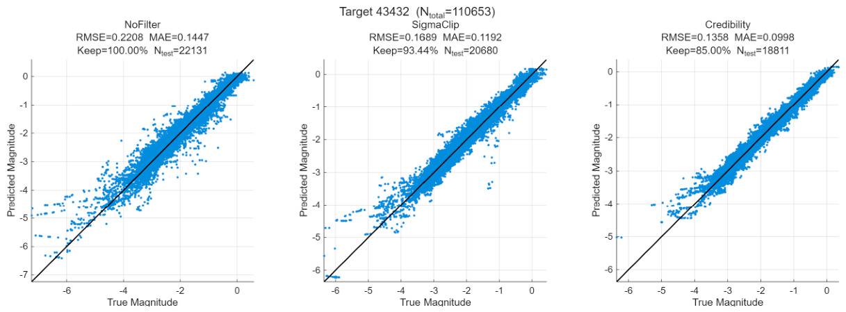
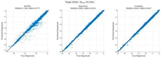
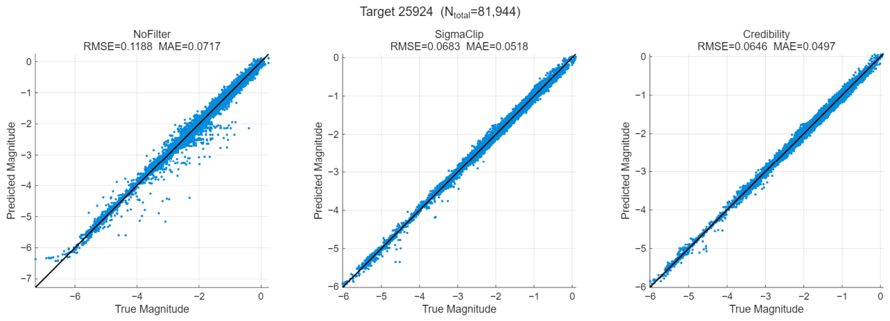
Figure 15 shows the predicted versus true magnitudes for target 25924 under the three strategies. Credibility-based filtering yields a tighter scatter around the diagonal and fewer large deviations than both No filtering and Sigma clipping, which is consistent with the lower RMSE and MAE reported in Table 7. The corresponding scatter plots for the other three targets are provided in Figure A1, Figure A2 and Figure A3 (Appendix A).
Figure 15.
Predicted versus true magnitude for target 25924 under three sample filtering strategies. From left to right: No filtering, Sigma clipping (2.5σ), and Credibility weighting. The black line is the 1:1 reference. RMSE and MAE are shown in each panel.
The hard rejection thresholds were not included in the sensitivity analysis. They are based on physical priors and conservative choices, and a systematic sensitivity analysis of these thresholds is left for future work.
5.7. Limitations and Applicability
The proposed framework is designed for routine high-frequency photometric observations of high-orbit targets with smooth, slowly varying light curves. It is most suitable for operational or recently retired GEO satellites, where the photometric variation is dominated by slow phase angle changes. For targets with fast rotation, tumbling, or strong specular flashes, the intrinsic short-timescale variability may be partially down-weighted; in such cases, a shorter smoothing window or a relaxed residual penalty is recommended. The method is not intended to replace physical modeling of rotational states, but to provide a general quality-control layer before such modeling. The framework is developed specifically for space-object photometry; its application to other celestial objects is not validated in this work and would require re-calibration of the thresholds and parameters.
6. Conclusions
In this paper, we proposed a quality assessment method that integrates hard rejection and multi-dimensional soft weighting for ground-based high-frequency photometric data of high-orbit targets, and constructed a hierarchical scoring system from the point level to the target level. The method operates along three dimensions—elevation angle, arc information content, and photometric smoothing residual—using robust statistics and truncated penalty techniques to generate continuous credibility weights between 0 and 1 for each observation point, while providing visual diagnosis via three-color scatter plots. Experimental results show that the hard rejection ratio is controlled within 3%, the weight distribution is in good agreement with the actual data quality, and the comprehensive credibility is concentrated in the high-credibility range, with low-weight points corresponding to physically interpretable scenarios such as transient arc edges and isolated jumps. The daily score effectively distinguishes the data quality of different observation days, and preliminary visual inspection suggests that the ranking results are consistent with the observed data quality trends; the target-level score provides a quantitative basis for cross-target comparisons.
The comprehensive credibility output by our method can be used as a filtering criterion in downstream models, as demonstrated by the improved RMSE and MAE in the ablation study. Using it as continuous sample weights in the loss function is a promising direction for future work. In future work, we will integrate an observation geometry calculation module to incorporate the contribution of phase angle variation to arc weights, and explore deeper applications of credibility information in physical model optimization.
Author Contributions
Conceptualization, C.X.; methodology, Y.L. (Yang Liu); software, Y.L. (Yang Liu); validation, Y.L. (Yang Liu); formal analysis, X.T., Q.Z. and Y.L. (Yao Lu); investigation, X.T., Q.Z. and Y.L. (Yao Lu); resources, C.X.; data curation, Y.L. (Yang Liu); writing—original draft preparation, Y.L. (Yang Liu); writing—review and editing, Y.L. (Yang Liu), C.X. and Y.Z.; visualization, Y.L. (Yang Liu); supervision, C.X. and Y.Z. All authors have read and agreed to the published version of the manuscript.
Funding
This research received no external funding.
Data Availability Statement
The data presented in this study are available on request from the corresponding author. The data are not publicly available due to the data policy of the National Astronomical Observatories, Chinese Academy of Sciences.
Acknowledgments
We would like to thank the National Astronomical Observatories, Chinese Academy of Sciences for the device measurement. In preparing this manuscript, we also used DeepSeek-V3 (DeepSeek, Hangzhou, China) to translate the initial Chinese draft into English. All AI-generated text was subsequently checked and corrected by us, and we take full responsibility for the final content.
Conflicts of Interest
The authors declare no conflict of interest.
Abbreviations
The following abbreviations are used in this manuscript:
| ACS | Advanced Camera for Surveys (Hubble Space Telescope instrument) |
| CALIFA | Calar Alto Legacy Integral Field Area Survey |
| DQF | Data Quality Flags |
| GEO | Geostationary Earth Orbit |
| HST | Hubble Space Telescope |
| SDSS | Sloan Digital Sky Survey |
| STScI | Space Telescope Science Institute |
| UTC | Coordinated Universal Time |
Appendix A
Figure A1.
Predicted versus true magnitude for target 32019 under three sample filtering strategies. From left to right: No filtering, Sigma clipping (2.5σ), and Credibility weighting. The black line is the 1:1 reference. RMSE and MAE are shown in each panel. The point counts in Figure A1 correspond to the subset of points that satisfy the additional input requirements of the downstream MLP model, which is slightly smaller than the total number of points after quality assessment reported in Table 3.
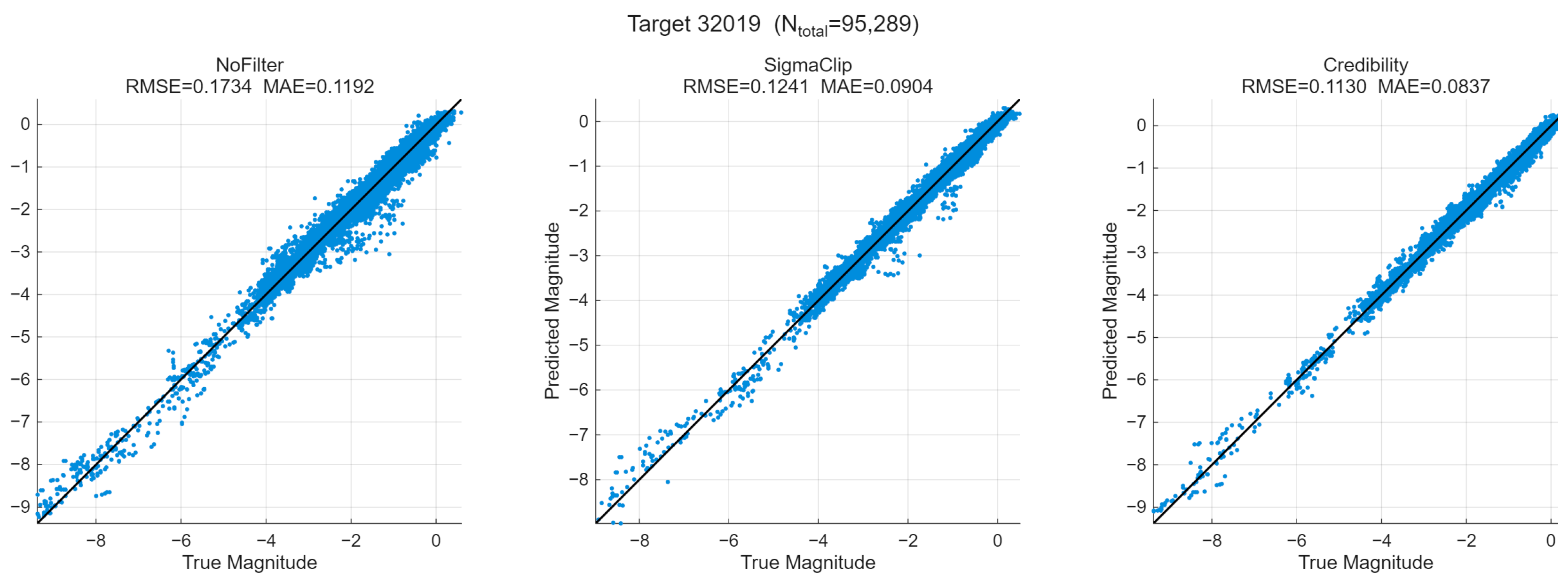
Figure A2.
Predicted versus true magnitude for target 41725 under three sample filtering strategies. From left to right: No filtering, Sigma clipping (2.5σ), and Credibility weighting. The black line is the 1:1 reference. RMSE and MAE are shown in each panel.
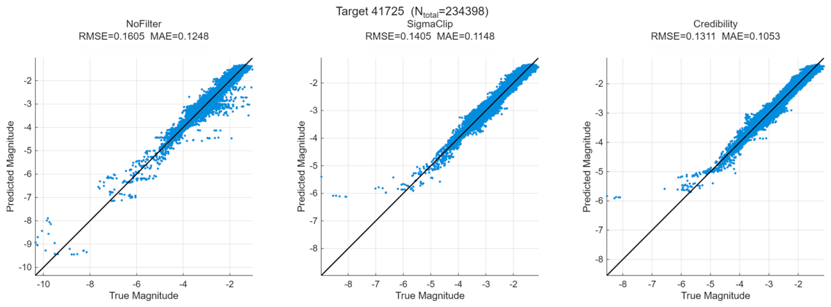
Figure A3.
Predicted versus true magnitude for target 43432 under three sample filtering strategies. From left to right: No filtering, Sigma clipping (2.5σ), and Credibility weighting. The black line is the 1:1 reference. RMSE and MAE are shown in each panel.
References
- Scott, R.L.; Thorsteinson, S.; Abbasi, V. On-Orbit Observations of Conjuncting Space Objects Prior to the Time of Closest Approach. J. Astronaut. Sci. 2020, 67, 1735–1754. [Google Scholar] [CrossRef] [Scilit]
- Tang, Y.J.; Jiang, X.J.; Lu, X.M.; Wei, J.Y.; Hu, J.Y. Photometric characteristics of mid-high orbit artificial satellites based on illumination reflection model. Acta Opt. Sin. 2010, 30, 763–767. (In Chinese) [Google Scholar] [CrossRef] [Scilit]
- Huang, S.; Zhao, J.; Xu, F.; Wang, L.; Song, T.; Cai, Y. Progress in Measurement and Calculation Methods of Atmospheric Effects on Telescope Image Quality. Chin. Astron. Astrophys. 2025, 49, 280–316. [Google Scholar] [CrossRef] [Scilit]
- Ouyang, P.X.; Chen, K.Y.; Guo, Y.M.; Rao, C.H. Spatiotemporal characteristics analysis of daytime sky background based on Hartmann wavefront sensor. Opt. Precis. Eng. 2025, 33, 3431–3440. (In Chinese) [Google Scholar] [CrossRef]
- Bi, X.; Chen, W.; Han, X.; Chen, K.; Yang, Y.; Li, J.; Qin, G.; Ge, J.; Zhang, H.; Willis, K. The Effect of Pointing Stability on Earth 2.0 Space Mission’s Photometry Precision. In Proceedings of the Space Telescopes and Instrumentation 2022: Optical, Infrared, and Millimeter Wave; Coyle, L.E., Perrin, M.D., Matsuura, S., Eds.; SPIE: Montréal, QC, Canada, 2022; p. 208. [Google Scholar]
- Tsuchikawa, T.; Endo, T.; Tsuji, H. Estimating Physical Properties of 3U CubeSat’s Rotation Based on Photometric Observations and Solar Illumination Modeling. In Proceedings of the Advanced Maui Optical and Space Surveillance (AMOS) Technologies Conference, Maui, HI, USA, 17–20 September 2024. [Google Scholar]
- DQ Flag Definitions. Available online: https://www.stsci.edu/home/hst/instrumentation/acs/data-analysis/dq-flag-definitions (accessed on 16 July 2026).
- Spectroscopic Data Quality Flags—SDSS-III. Available online: https://sdss3.org/dr10/spectro/spectro_catalog_quality.php (accessed on 16 July 2026).
- Sánchez, S.F.; García-Benito, R.; Zibetti, S.; Walcher, C.J.; Husemann, B.; Mendoza, M.A.; Galbany, L.; Falcón-Barroso, J.; Mast, D.; Aceituno, J.; et al. CALIFA, the Calar Alto Legacy Integral Field Area Survey: IV. Third Public Data Release. Astron. Astrophys. 2016, 594, A36. [Google Scholar] [CrossRef] [Scilit]
- Ngeow, C.; Kanbur, S. Nonlinear Period-Luminosity Relation for the Large Magellanic Cloud Cepheids: Myths and Truths. Astrophys. J. 2006, 650, 180–188. [Google Scholar] [CrossRef] [Scilit] [PubMed]
- Howell, S.B. Handbook of CCD Astronomy, 2nd ed.; Cambridge University Press: Cambridge, UK, 2006; ISBN 978-0-521-85215-9. [Google Scholar]
- Creaner, O.; Nolan, K.; Hickey, E.; Smith, N. The Locus Algorithm: A Novel Technique for Identifying Optimised Pointings for Differential Photometry. Astron. Comput. 2022, 38, 100537. [Google Scholar] [CrossRef] [Scilit]
- Osborn, J.; Föhring, D.; Dhillon, V.S.; Wilson, R.W. Atmospheric Scintillation in Astronomical Photometry. Mon. Not. R. Astron. Soc. 2015, 452, 1707–1716. [Google Scholar] [CrossRef] [Scilit]
- Tang, Y.J.; Jiang, X.J.; Wang, J.F.; Wei, J.Y.; Hu, J.Y. Diffuse reflection light curve characteristics of three-axis stabilized GEO satellites. Acta Photon. Sin. 2009, 38, 2863–2866. (In Chinese) [Google Scholar]
- Press, W.H.; Teukolsky, S.A.; Vetterling, W.T.; Flannery, B.P. Numerical Recipes: The Art of Scientific Computing, 3rd ed.; Cambridge University Press: Cambridge, UK, 2007; ISBN 978-0-521-88068-8. [Google Scholar]
- Xia, P.P.; Wang, Z.Q.; Li, H.W.; Deng, Y.T.; Wang, X.J. Speed control of K-mirror for 2 m telescope based on adaptive active disturbance rejection control. Infrared Laser Eng. 2018, 47, 233–240. (In Chinese) [Google Scholar] [CrossRef] [Scilit]
- Green, D.W.E. Magnitude corrections for atmospheric extinction. Int. Comet Q. 1992, 14, 55. [Google Scholar]
- Handler, G. Variable Central Stars of Young Planetary Nebulae: A Photometric Study of the Central Star of M 2–54. Astron. Astrophys. Suppl. Ser. 1999, 135, 493–498. [Google Scholar] [CrossRef] [Scilit]
- Choi, J.; Jo, J.-H.; Choi, Y.-J.; Cho, G.-I.; Kim, J.-H.; Bae, Y.-H.; Yim, H.-S.; Moon, H.-K.; Park, J.-H. A Study on the Strategies of the Positioning of a Satellite on Observed Images by the Astronomical Telescope and the Observation and Initial Orbit Determination of Unidentified Space Objects. J. Astron. Space Sci. 2011, 28, 333–344. [Google Scholar] [CrossRef] [Scilit]
- Xu, C.; Zhang, Y.S.; Zhang, F.; Liu, C.H. Seasonal flare phenomenon of solar panels on three-axis stabilized geostationary orbit satellites. Acta Opt. Sin. 2018, 38, 322–329. (In Chinese) [Google Scholar]
- Rousseeuw, P.; Croux, C. Alternatives to Median Absolute Deviation. J. Am. Stat. Assoc. 1993, 88, 1273–1283. [Google Scholar] [CrossRef]
- Maronna, R.A.; Martin, R.D.; Yohai, V.J.; Salibián-Barrera, M. Robust Statistics: Theory and Methods (with R), 2nd ed.; John Wiley & Sons: Hoboken, NJ, USA, 2019; ISBN 978-1-119-21468-7. [Google Scholar]
- Hair, J.F., Jr.; Black, W.C.; Babin, B.J.; Anderson, R.E. Multivariate Data Analysis, 7th ed.; Prentice Hall: Upper Saddle River, NJ, USA, 2010; ISBN 978-0-13-813263-7. [Google Scholar]

Disclaimer/Publisher’s Note: The statements, opinions and data contained in all publications are solely those of the individual author(s) and contributor(s) and not of MDPI and/or the editor(s). MDPI and/or the editor(s) disclaim responsibility for any injury to people or property resulting from any ideas, methods, instructions or products referred to in the content. |
© 2026 by the authors. Licensee MDPI, Basel, Switzerland. This article is an open access article distributed under the terms and conditions of the Creative Commons Attribution (CC BY) license.